28
Wind-driven circulation II ●Wind pattern and oceanic gyres ●Sverdrup Relation ●Vorticity Equation
| Date post: | 24-Dec-2015 |
| Category: |
Documents |
| Upload: | deborah-harrison |
| View: | 217 times |
| Download: | 0 times |

Wind-driven circulation II
●Wind pattern and oceanic gyres
●Sverdrup Relation
●Vorticity Equation


Surface current measurement from ship drift
Current measurements are harder to make than T&SThe data are much sparse.

Surface current observations

Surface current observations

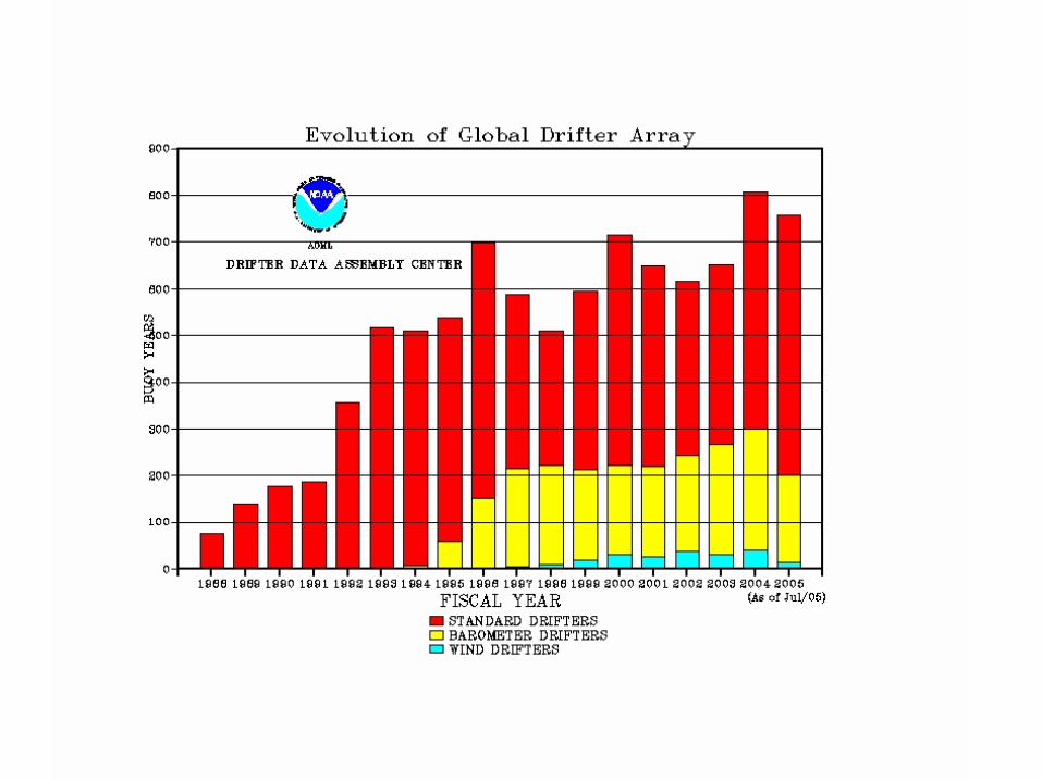

Drifting Buoy Data Assembly Center, Miami, Florida Atlantic Oceanographic and Meteorological Laboratory, NOAA

Annual Mean Surface CurrentPacific Ocean, 1995-2003
Drifting Buoy Data Assembly Center, Miami, Florida Atlantic Oceanographic and Meteorological Laboratory, NOAA


Schematic picture of the major surface currents of the world oceans
Note the anticyclonic circulation in the subtropics (the subtropical gyres)

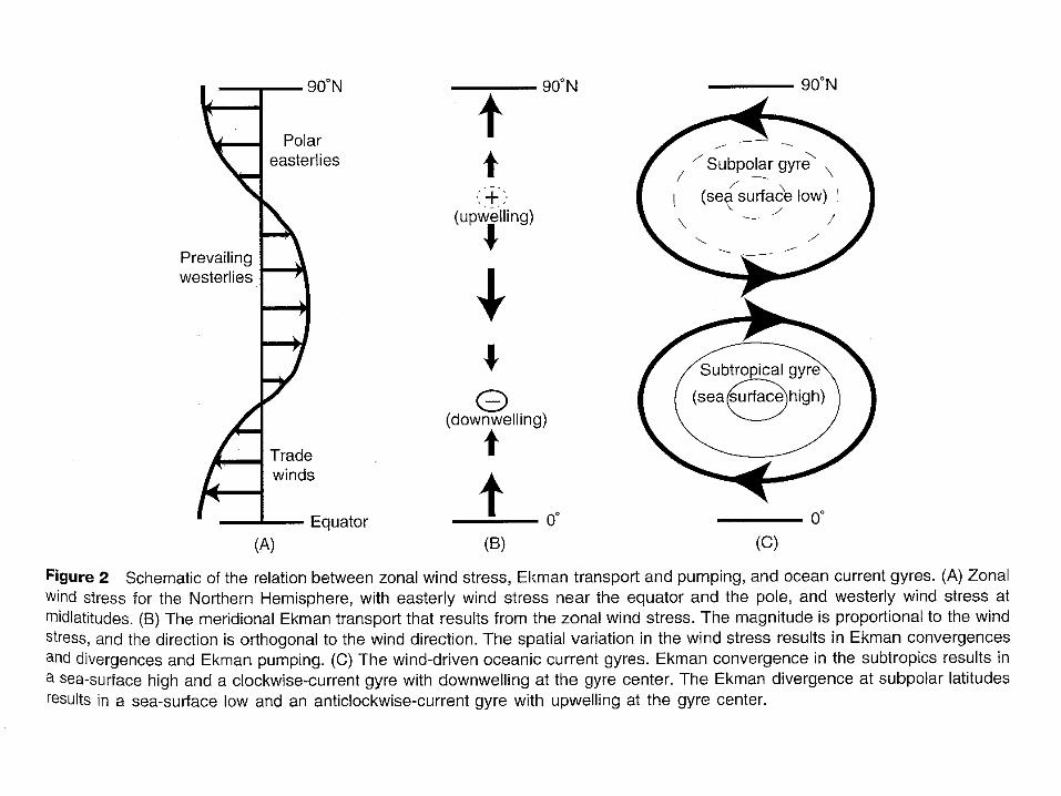
Relation between surface winds and subtropical gyres

Surface winds and oceanic gyres: A more realistic view
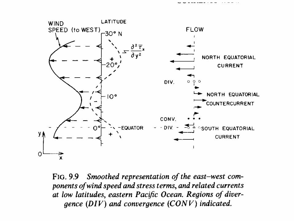
Note that the North Equatorial Counter Current (NECC) is against the direction of prevailing wind.

Mean surface current tropical Atlantic Ocean
Note the North Equatorial Counter Current (NECC)

Sverdrup RelationConsider the following balance in an ocean of depth h of flat
bottom
∫ +=+∫=∂∂
− −
000
0
hxyx
hfMvdzfdz
xp ττρ
(1)
∫ +−=+∫−=∂∂
− −
000
0
hyxy
hfMudzfdz
yp ττρ
(2)
∫=−
0
hx udzM ρ
∫=−
0
hy vdzM ρ
zvf
xp x
∂∂+=
∂∂ τρ
zuf
yp y
∂∂+−=
∂∂ τρ
Integrating vertically from –h to 0 for both (1) and (2), we have(neglecting bottom stress and surface height change)
where
(3)
(4)
are total zonal and meridional transport of mass
sum of geostrophic and ageostropic transports

Differentiating , we have
000=
∂∂−
∂∂+−
∂∂+
∂∂−
⎟⎟⎟
⎠
⎞
⎜⎜⎜
⎝
⎛
yxdydfM
yM
xMf xy
yyx ττ
€ P=pdz−h0∫Define We have
€ ∂p∂xdz=∂∂xpdz−h0∫ ⎡ ⎣ ⎢ ⎤ ⎦ ⎥=∂P∂x−h0∫
€ ∂P∂x=fMy+τx0€
∂P∂y=−fMx+τy0(3) and (4) can be written as
(5) (6)
€ ∂6()∂x−∂5()∂y
€ ∂2P∂y∂x−∂2P∂x∂y=−f∂Mx∂x+∂τy0∂x−f∂My∂y−Mydfdy−∂τx0∂y=0
000=
∂∂−
∂∂+−
∂∂+
∂∂−
⎟⎟⎟
⎠
⎞
⎜⎜⎜
⎝
⎛
yxdydfM
yM
xMf xy
yyx ττ
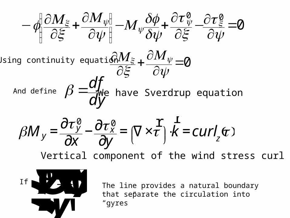
Using continuity equation 0=∂∂+
∂∂
yM
xM yx
And define
dydf=β
( )ττττβz
xyy curlk
yxM =⋅×∇=
∂∂−
∂∂= ⎟
⎠⎞⎜
⎝⎛
rr00
Vertical component of the wind stress curl
We have Sverdrup equation
€ ∂τy0∂x−∂τx0∂y=0If
€ My=0The line provides a natural boundary that separate the circulation into “gyres”

€ My=Myg+MyEis the total meridional mass transport
€ Myg=ρvgdz=1f∂p∂xdz=1f∂P∂x−h0∫−h0∫ Geostrophic transport
€ MyE=ρvEdz=−τx0f−h0∫ Ekman transport
Order of magnitude example:At 35oN, -4 s-1, β2 10-11 m-1 s-1, assume τx10-1 Nm-2 τy=0
€ curlzτ()=−∂τx0∂y≈−10−1Nm−21000km≈−10−7Nm−3
€ MyE=−τx0f≈−103kgm−1s−1
€ My=Myg+MyE=curlzτ()β≈−10−72×10−11=−5×10³kgm−1s−1€ Myg=−4×10³kgm−1s−1

Alternative derivation of Sverdrup Relation
xp
gfv ∂∂=
ρ
ypfu
g ∂∂−=
ρ
Construct vorticity equation from geostrophic balance
(1)
(2)
zw
fv gg ∂
∂=β
Integrating over the whole ocean depth, we have
€ f∂ug∂x+f∂vg∂y+βvg=−1ρ∂2p∂y∂x+1ρ∂2p∂x∂y=0€
∂2()∂x+∂1()∂y€ βvg=−f∂ug∂x+∂vg∂y ⎛ ⎝ ⎜ ⎞ ⎠ ⎟=f∂wg∂z
Assume ρ=constant
€ βVg=βvgdz=fwgz=0()−wgz=−h()[ ]−h0∫

∫ ==−
0
hEgg fwdzvV ββ
kf
wE
rr⋅×∇=⎟⎟⎟⎟
⎠
⎞
⎜⎜⎜⎜
⎝
⎛
⎟⎟⎟
⎠
⎞
⎜⎜⎜
⎝
⎛
ρτ
where is the entrainment rate from the surface Ekman layer
⎟⎟⎠
⎞⎜⎜⎝
⎛=+= ρτ
β curlVVV Eg1
The Sverdrup transport is the total of geostrophic and Ekman transport.The indirectly driven Vg may be much larger than VE.
( )6tan ≈===
⎟⎟⎟
⎠
⎞
⎜⎜⎜
⎝
⎛
⎟⎟⎟⎟⎟
⎠
⎞
⎜⎜⎜⎜⎜
⎝
⎛
ϕβτ
βτ
LR
LfO
f
curlO
VV
E
gat 45oN
€ βVg=βvgdz=fwgz=0()−wgz=−h()[ ]−h0∫
€ wgz=0()=wE€ wgz=−h()≈0€ Vg=fβρ∂∂xτyf ⎛ ⎝ ⎜ ⎞ ⎠ ⎟−∂∂yτxf ⎛ ⎝ ⎜ ⎞ ⎠ ⎟ ⎛ ⎝ ⎜ ⎞ ⎠ ⎟=fρβ1f∂τy∂x−1f∂τx∂y+βτxf2 ⎛ ⎝ ⎜ ⎞ ⎠ ⎟€ Vg=1ρβ∂τy∂x−∂τx∂y+βτxf ⎛ ⎝ ⎜ ⎞ ⎠ ⎟=1ρβ∂τy∂x−∂τx∂y ⎛ ⎝ ⎜ ⎞ ⎠ ⎟−VE

€ βMy=∂τy0∂x−∂τx0∂y
€ f=2Ωsinφ€ dy=Rdφ( )
⎟⎠⎞⎜
⎝⎛ Ω
=R
zcurlM y
ϕ
τ
cos2then
( ) ( )⎟⎟
⎠
⎞
⎜⎜
⎝
⎛⎟⎠⎞⎜
⎝⎛ −∂
∂Ω−=∂
∂−=∂∂ τϕτϕ zz
yx curlcurly
RyM
xM tan
cos21
€ β=dfdy=d2Ωsinφ( )Rdφ=2ΩsinφR

Since , we have
⎟⎟⎟
⎠
⎞
⎜⎜⎜
⎝
⎛
∂
∂+
∂∂
Ω−=∂∂
yyR
xM xxx
τϕ
τϕ
tancos21
2
2
set x =0 at the eastern boundary,
⎟⎟⎟
⎠
⎞
⎜⎜⎜
⎝
⎛
∫ ∫∂∂+∂
∂Ω−=
0 0
2
2tan
cos21
x x
xxx dx
ydx
yRM τϕτ
ϕ
yRM x
y ∂∂
Ω= τϕcos2
€ τy≈0
Further assume€ τx≈τxy()In the trade wind and equatorial zones, the 2nd derivative term dominates:
€ Mx≈xR2Ωcosφ∂2τx∂y2€ Mx=x2Ωcosφ∂τx∂ytanφ+∂2τx∂y2R ⎛ ⎝ ⎜ ⎞ ⎠ ⎟


Mass Transport
Since 0=∂∂+
∂∂
yM
xM yx
Let y
M x ∂∂−= ψ
,
xM y ∂
∂= ψ,
( )βτψ zcurl
x=
∂∂
( )∫=0
x
z dxcurlβτψ
where ψ is stream function.
Problem: only one boundary condition can be satisfied.

1 Sverdrup (Sv) =106 m3/s