Page 1
Energies 2013, 6, 696-716; doi:10.3390/en6020696
energies ISSN 1996-1073
www.mdpi.com/journal/energies
Article
Wind Farm Wake: The Horns Rev Photo Case
Charlotte Bay Hasager 1,
*, Leif Rasmussen 2, Alfredo Peña
1, Leo E. Jensen
3 and
Pierre-Elouan Réthoré 1
1 Technical University of Denmark, DTU Wind Energy, Risø Campus, Frederiksborgvej 399,
4000 Roskilde, Denmark; E-Mails: [email protected] (A.P.); [email protected] (P.-E.R.) 2 Retired Senior Meteorologist from Danish Meteorological Institute, Lyngbyvej 100,
2100 København Ø, Denmark; E-Mail: [email protected] 3 DONG Energy, Kraftværksvej 53, 7000 Fredericia, Denmark; E-Mail: [email protected]
* Author to whom correspondence should be addressed; E-Mail: [email protected] ;
Tel.: +45-4677-5014; Fax: +45-4677-5970.
Received: 3 November 2012; in revised form: 21 January 2013 / Accepted: 25 January 2013 /
Published: 5 February 2013
Abstract: The aim of the paper is to examine the nowadays well-known wind farm wake
photographs taken on 12 February 2008 at the offshore Horns Rev 1 wind farm. The
meteorological conditions are described from observations from several satellite sensors
quantifying clouds, surface wind vectors and sea surface temperature as well as
ground-based information at and near the wind farm, including Supervisory Control and
Data Acquisition (SCADA) data. The SCADA data reveal that the case of fog formation
occurred 12 February 2008 on the 10:10 UTC. The fog formation is due to very special
atmospheric conditions where a layer of cold humid air above a warmer sea surface
re-condensates to fog in the wake of the turbines. The process is fed by warm humid air
up-drafted from below in the counter-rotating swirl generated by the clock-wise rotating
rotors. The condensation appears to take place primarily in the wake regions with relatively
high axial velocities and high turbulent kinetic energy. The wind speed is near cut-in and
most turbines produce very little power. The rotational pattern of spiraling bands produces
the large-scale structure of the wake fog.
Keywords: wind farm wake; cloud; fog; satellite; met-ocean conditions; wake model
OPEN ACCESS
Page 2
Energies 2013, 6 697
1. Introduction
The Horns Rev 1 wind farm is located in the North Sea at about 14 to 20 km offshore from the
Danish coastline (Figure 1).
Figure 1. Location of the Horns Rev 1 wind farm in the North Sea.
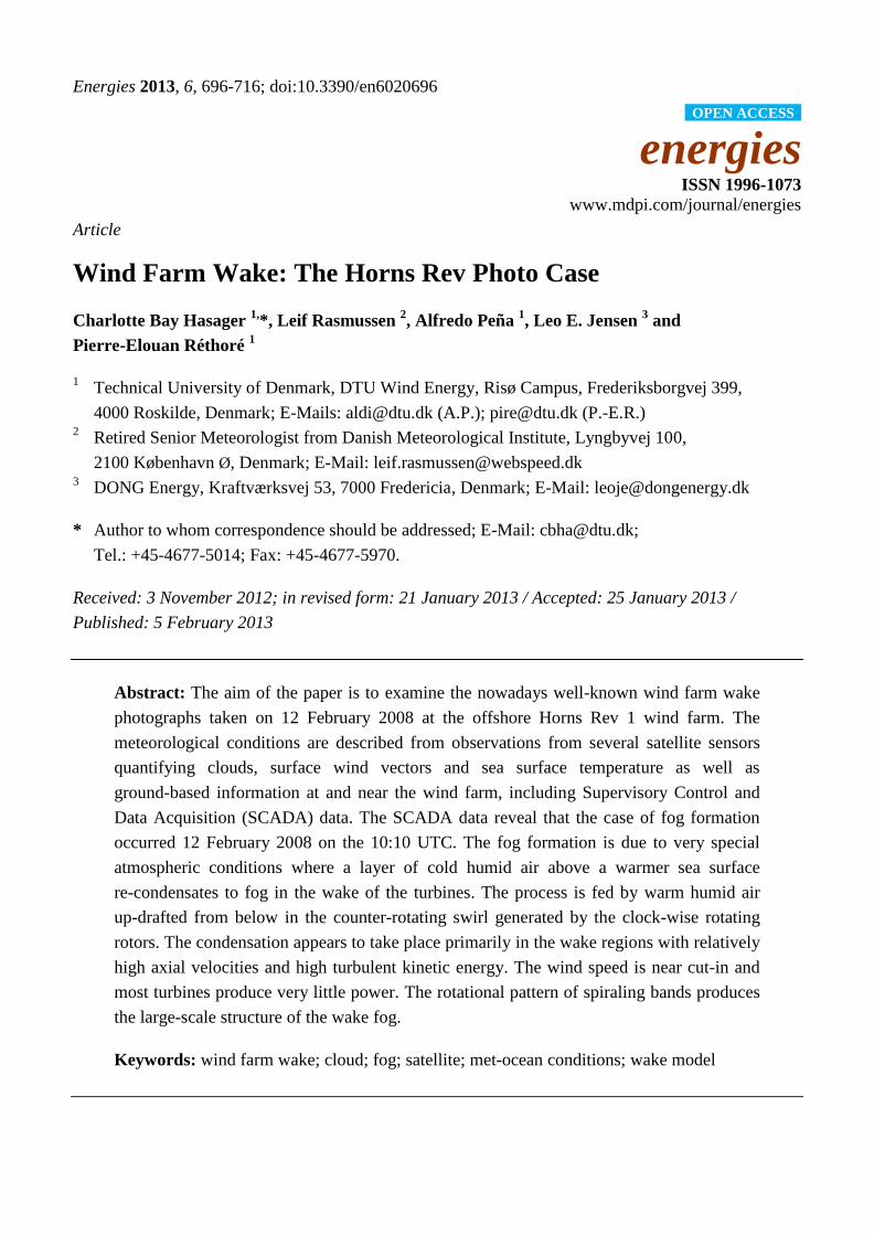
The wake photographs taken at the offshore wind farm at Horns Rev 1 are well known in the wind
energy community. They illustrate the wind turbine shadow effect in an attractive manner. The two
photographs were taken by the pilot from the window of the helicopter on its way out to the oil rigs in
the North Sea at an altitude around 1 to 3 km on 12 February 2008 at around 10:10 UTC. The first
photo [Figure 2(a)] was taken from the southeast and the second [Figure 2(b)] from the south.
The aim of the paper is to examine the case from combined satellite data, local meteorological
observations, radio-sounding data and Supervisory Control and Data Acquisition (SCADA) data from
the wind farm. The weather conditions are described and an interpretation of the origin of the fog is
provided. Furthermore advanced wake modeling with Computational Fluid Dynamics (CFD) using
Detached Eddy Simulation (DES) of a full wind turbine rotor is included to detail the physical
processes in the wake of the wind turbines in relation to the formation and dispersion of fog. The
meteorological observations, the operation of the wind turbines and the mechanically-driven
convection are discussed.
Page 3
Energies 2013, 6 698
Figure 2. (a) Upper panel: Photograph of the Horns Rev 1 offshore wind farm 12 February
2008 at around 10:10 UTC seen from the southeast. (b) Lower panel: Same as (a) but
shortly after, seen from the south. Courtesy: Vattenfall. Photographer is Christian Steiness.
2. Fog Formation and Dispersal
The physical mechanisms for fog formation include three primary processes: cooling, moistening
and vertical mixing of air parcels with different temperatures and humidity. Advection fog, frontal fog
and radiation fog are the three major types of fog [1].
a
b
Page 4
Energies 2013, 6 699
Advection fog can be either warm-water advection fog with cold air flowing over warm water, or
cold-water advection fog with warm air flowing over cold water. When cold humid air is advected
over a much warmer water surface, there will be the possibility of upward mixing of warm saturated
air from the surface into the cooler layer. This can cause a super-saturated mixture to develop and
condense as fog or sea smoke. In contrast, cold-water advection fog occurs when warm moist air flows
across colder water and the dew-point temperature is reached such that fog forms.
Frontal fog is usually caused by evaporation of warm rain falling through a layer of cold air near the
ground, or eventually by mixing of moist air masses with different temperatures leading to saturation.
Radiation fog forms when humid air near the surface cools due to radiative cooling and light winds
cause turbulent warming near the surface. The fog is then maintained through further cooling caused
by long-wave radiative flux divergence at the top of the fog layer. Fog and droplets form and
gravitational droplets settle. The process is typical for marshland, lakes and other depressions in the
landscape during evening and night [2].
The processes for formation and dispersal of fog are governed by a delicate balance of
thermodynamic and dynamical variables. In urban and sub-urban areas the condensation to fog can be
stimulated by nuclei such that smaller droplets are formed than those typical in cleaner air as over the
ocean. Fog disperses as dryer or warmer air is mixed into the fog and dilutes the moisture
concentration. Increasing winds thwart fog formation by increasing turbulent mixing [2].
According to [3] the fog at the Horns Rev 1 wind farm is described as mixing fog formed when two
nearly saturated layers of air masses with different temperatures are mixed. The explanation given is
that condensation starts when warmer air is mixed in due to turbulence produced by the turning
turbines. This is discussed in Section 6.
3. Data from Satellites and Weather Conditions
3.1. Satellite Maps
Earth observation satellites provide images of the atmospheric and oceanographic conditions.
Satellite maps of the clouds, ocean winds and sea surface temperatures are presented and described to
detail the met-ocean conditions on the specific morning.
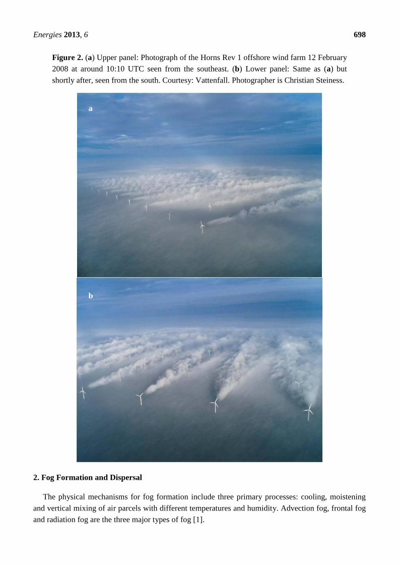
On-board the Terra satellite belonging to National Aeronautics and Space Administration (NASA)
is the instrument MODIS, the Moderate Resolution Imaging Spectroradiometer with 36 channels from
visual to thermal infrared. On 12 February 2008 Terra mapped the North Sea at 10:07 UTC
[Figure 3(a)].
Three other satellites confirm the cloud cover in the wind farm area in the late morning. These
include NOAA AVHRR (National Ocean and Atmosphere Administration, Advanced Very High
Resolution Radiometer) at 11:43 UTC and Aqua MODIS at 11:50 UTC. The geostationary satellite
Meteosat belonging to EUMETSAT (European Organisation for the Exploitation of Meteorological
Satellites) shows cloud cover at 12:00 UTC. At 12:00 UTC, low, homogeneous, stratiform clouds
covered Horns Rev. Due to the low viewing angle of Meteosat a rather thick appearance of clouds
prevails while the NOAA AVHRR and MODIS images taken at a steeper angle reveal a more variable
cloud structure. The latter may explain that the wind farm is sunlit in the photos.
Page 5
Energies 2013, 6 700
The Advanced Scatterometer ASCAT belonging to EUMETSAT observes ocean winds and
direction. On the 12 February 2008 at 09:16 UTC ocean surface wind vectors near Horns Rev were
from the south ~5 ms−1
[Figure 3(b)]. ASCAT was in the descending mode. At 20:45 UTC ASCAT in
ascending mode observed similar wind conditions. The QuikSCAT satellite with the SeaWinds
scatterometer on-board belongs to NASA. QuikSCAT observed ocean wind speed and wind direction
at 05:00 UTC with weak winds around 3 to 5 ms−1
from the south near Horns Rev. The QuikSCAT
evening wind map from 18:54 UTC showed similar wind conditions (see [4]). QuikSCAT and ASCAT
are based on active microwave radar scatterometry, thus the mapping of ocean wind vectors is done
day and night and in cloudy conditions.
Figure 3. (a) Left panel: Cloud cover over the North Sea observed from MODIS Terra on
12 February 2008 at 10:07 UTC from NERC Satellite Receiving Station, Dundee
University, Scotland at www.sat.dundee.ac.uk. (b) Right panel: Ocean surface vector
winds observed from ASCAT at 12 February 2008 at 09:16 UTC. The map is produced by
the EUMETSAT OSI SAF. The red circles indicate the location of the Horns Rev 1
wind farm. The arrow shows 10 ms−1
.
Despite the cloud cover [Figure 3(a)], the ocean surface vector winds are retrieved [Figure 3(b)].
The observations from QuikSCAT and ASCAT are both valid at 10 m above sea level and compare
well with observations from a meteorological mast near the Horns Rev 1 wind farm. The
meteorological mast M6 is located closer to land than the scatterometers cover. Please refer to
section 3.3 for further details on the local observations.
Page 6
Energies 2013, 6 701
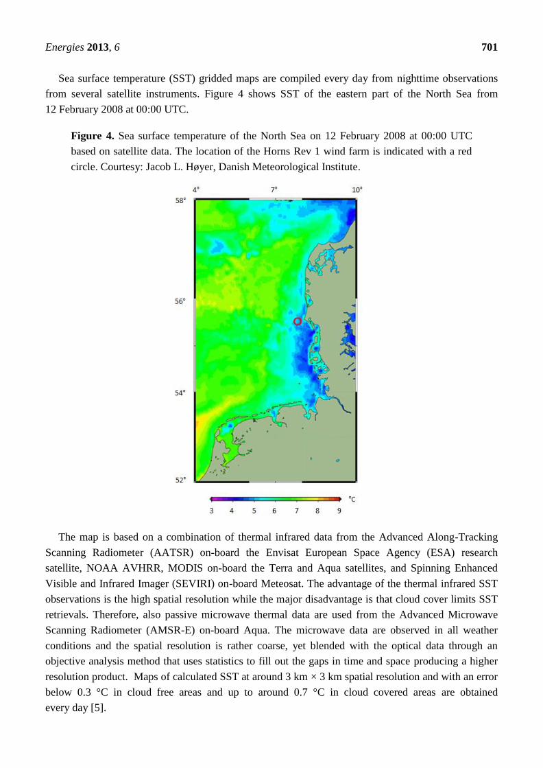
Sea surface temperature (SST) gridded maps are compiled every day from nighttime observations
from several satellite instruments. Figure 4 shows SST of the eastern part of the North Sea from
12 February 2008 at 00:00 UTC.
Figure 4. Sea surface temperature of the North Sea on 12 February 2008 at 00:00 UTC
based on satellite data. The location of the Horns Rev 1 wind farm is indicated with a red
circle. Courtesy: Jacob L. Høyer, Danish Meteorological Institute.
The map is based on a combination of thermal infrared data from the Advanced Along-Tracking
Scanning Radiometer (AATSR) on-board the Envisat European Space Agency (ESA) research
satellite, NOAA AVHRR, MODIS on-board the Terra and Aqua satellites, and Spinning Enhanced
Visible and Infrared Imager (SEVIRI) on-board Meteosat. The advantage of the thermal infrared SST
observations is the high spatial resolution while the major disadvantage is that cloud cover limits SST
retrievals. Therefore, also passive microwave thermal data are used from the Advanced Microwave
Scanning Radiometer (AMSR-E) on-board Aqua. The microwave data are observed in all weather
conditions and the spatial resolution is rather coarse, yet blended with the optical data through an
objective analysis method that uses statistics to fill out the gaps in time and space producing a higher
resolution product. Maps of calculated SST at around 3 km × 3 km spatial resolution and with an error
below 0.3 °C in cloud free areas and up to around 0.7 °C in cloud covered areas are obtained
every day [5].
Page 7
Energies 2013, 6 702
The gridded SST map shows temperatures around 5 °C near Horns Rev. This compares well with
the calculated sea temperature of the upper model layer of the Danish Meteorological Institute (DMI)
regional three-dimensional ocean model representing 4 m depth. According to the DMI ocean
model [6] and the satellite-based SST map, the water was colder near coast but in general the sea was
warmer than the overlying air. The SST observations and ocean model results further compare very
well to an observation of sea temperature of 4.7 °C at 3 m depth at the meteorological masts near the
wind farm. The masts were operated by DONG energy and Vattenfall. There is a list of data in
the Appendix.
3.2. Weather Conditions
The weather condition in the morning of 12 February 2008 was characterized by very high pressure
in Eastern Europe that had spread towards southern Scandinavia resulting in a separate high pressure
centre around 1040 hPa in eastern Denmark. This pattern caused light winds to blow from south (S)
and southeast (SE) in the wind farm area. Subsidence in the high pressure area formed a temperature
inversion, which, however, was at the same time characterized as a frontal inversion as a shallow cold
front arrived from northeast (NE) the previous day. The air mass behind the front was of maritime
origin, advected from the Norwegian Sea along the northern edge of the high pressure area. Crossing
Norway and Sweden on its way to Denmark and the continent it maintained its maritime properties,
and cooling from the surface made its humidity condense to widespread fog or low stratus cloud below
the inversion [Figure 3(a)]. Clouds or fog reveal clearly the propagation of a cold and moist air mass.
Just west of Horns Rev the cloudiness looks dense in Figure 3(a), in agreement with the photos in
Figure 2. In the latter it is possible to distinguish stratiform clouds in the distance. Further west and
even around and east of the wind farm warming from below has made the air mass break up into a
cellular pattern revealing a vertical mixing process with a partly change of the lapse rate from a wet
adiabatic to a dry or near dry adiabatic rate [Figure 3(a)]. The cellular pattern implies that the clouds
dissolve locally, including in the wind farm area. However, the air mass below the inversion stays
rather moist. Therefore sea smoke develops over the warm sea surface (Figure 2), and clouds are
restored in its upper part. The fog formation at the wind farm is not distinguishable in the MODIS
image [Figure 3(a)].
With prevailing winds from the south and southeast, the radio-sounding in Schleswig in northern
Germany around 150 km to the SE of the wind farm is assumed to be fairly representative of the air
mass over Horns Rev. The soundings reveal a surface inversion on 11 February at 00:00 UTC
gradually lifting to a frontal inversion (cf. the change of wind direction with height implying cold air
advection). The inversion lifted from around 300 m height at 12.00 UTC on 11 February to 600 m at
00:00 UTC 12 February and to 750 m at 12:00 UTC [7]. The sounding from 12 February at 00:00 UTC
is shown in Figure 5.
The air was saturated (i.e., with solid cloud) and the lapse rate stable or wet-adiabatic governed
below the inversion becoming dry-adiabatic during the day. Dry and warmer air aloft reflects
subsidence within the anticyclone.
Page 8
Energies 2013, 6 703
Figure 5. Radiosounding data from Schleswig from 12 February 2008 at 00:00 UTC.
From [7].
Increasing cloud thickness at two meteorological stations located east (E) and south-southeast
(SSE) of Horns Rev, respectively, Esbjerg Airport 43 km to the E [8] and List 65 km to the SSE [9], is
thought to be the reason for slightly increasing surface temperatures. At both stations the air
temperature increased from around 2 °C to 4 °C from the previous day to 12 February associated with
continuous fog or a very low cloud base and periods with drizzle.
3.3. Meteorological Conditions Observed at the Offshore Meteorological Masts
Near the Horns Rev 1 wind farm the local meteorological conditions were observed at two
meteorological masts M6 and M7 (see the location of M6 in Figure 10). M7 is located 4 km east of
M6. The wind profiles from M6 are graphed in Figure 6 for three 10-min periods: Before, at and after
the photographs. The wind profiles show slightly unstable conditions. Furthermore, the turbulence
intensity is observed to be ~17% at 70 m, ~16% at 40 m and ~18% at 30 m which also indicates
unstable conditions. The observations from 70 m are from a top-mounted cup anemometer whereas the
observations from 40 m and 30 m are from boom-mounted cup anemometers at the northwest booms
(see [10] for details). Thus the wind speed and turbulence intensity data may be influenced by the
mast and booms.
Page 9
Energies 2013, 6 704
Figure 6. Wind profiles observed at M6 on 12 February 2008 at 10:00 UTC (red), 10:10
UTC (black) and 10:20 UTC (blue) at three heights above sea level (ASL). Data are from
DONG Energy and Vattenfall.
Figure 7 shows the wind speeds, wind directions, air temperatures, and the potential temperature
difference from midnight to noon on 12 February 2008. The wind speeds are nearly constant and low,
~4–5 ms−1
, whereas the wind directions change from ~140° to ~190°. During the night the air
temperatures are below 2.5 °C. From 5:00 to 7:00 UTC the temperatures increase one degree and
thereafter the air temperatures are nearly constant ~3.5 °C. The water temperature at 3 m depth is
constantly 4.7 °C (not shown) but the potential temperature difference between 64 m and −3 m is
shown and the case is seen to be unstable. The pressure is ~1037 hPa and constant (not shown). For all
parameters observed there are very little differences between observations from M6 and M7. At both
masts air temperatures at 16 m are observed and the potential temperature difference between 64 m
and 16 m is nearly constant ~0.2 °C before 6 a.m. and thereafter nearly constant ~0.1 °C (not shown).
The local unstable conditions indicate that the stability decreases from a wet-adiabatic to a near
dry-adiabatic layering. The fog that had covered the entire area is disappearing due to this change in
the adiabatic situation. The thinning of the fog takes place from the top towards the bottom of the
inversion. Only sea smoke in a shallow layer of 5 to 10 m near the ocean surface remained
(Figure 2). [3] described the sea smoke as a result of a colder humid air advected over a warmer sea
surface. This explanation is supported by the meteorological observations near the wind farm. During
the entire morning the air temperature remained lower than the sea temperature, and vertical mixing to
a certain height might easily be achieved. Selected data from M6 are listed in the Appendix.
4. Wake Model Results from CFD DES
The distance in the turbine wakes at which the first condensation takes place is around 50 to 100 m
downstream centered at the nacelle position (Figure 2). To gain further insight to the physical
properties in the turbine wake field, CFD model results on axial velocity, turbulent kinetic energy
(TKE), vertical velocity and pressure are investigated.
Page 10
Energies 2013, 6 705
Figure 7. Meteorological conditions observed at M6 and M7 during 12 h on 12 February
2008. (a) Upper panel: Wind speeds at M6 (––) at 70 m and M7 (- -) at 60 m. Wind
directions: M6 (––) and M7 (- -) both at 68 m; (b) Lower panel: Air temperatures at
M6 (––) and M7 (- -) both at 64 m. Potential temperature difference between 64 m and
−3 m at M6 (––) and M7 (- -). The thin vertical line indicates the time of the photographs.
Data are from DONG Energy and Vattenfall.
(a)
(b)
The result on the axial velocity in the wake from the simulation with a full rotor DES (with an
overset mesh method) of a NEG Micon NM80 turbine in clock-wise rotation with a velocity at hub
height of 8 ms−1
and with a vertical shear on the axial wind velocity is shown in Figure 8. For more
information about the simulation see the original article for which the simulation was carried out [11].
The streamline visible shows how a mass of air located under the hub height of the rotor would be
displaced to a higher position vertically due to the wake rotation.
Page 11
Energies 2013, 6 706
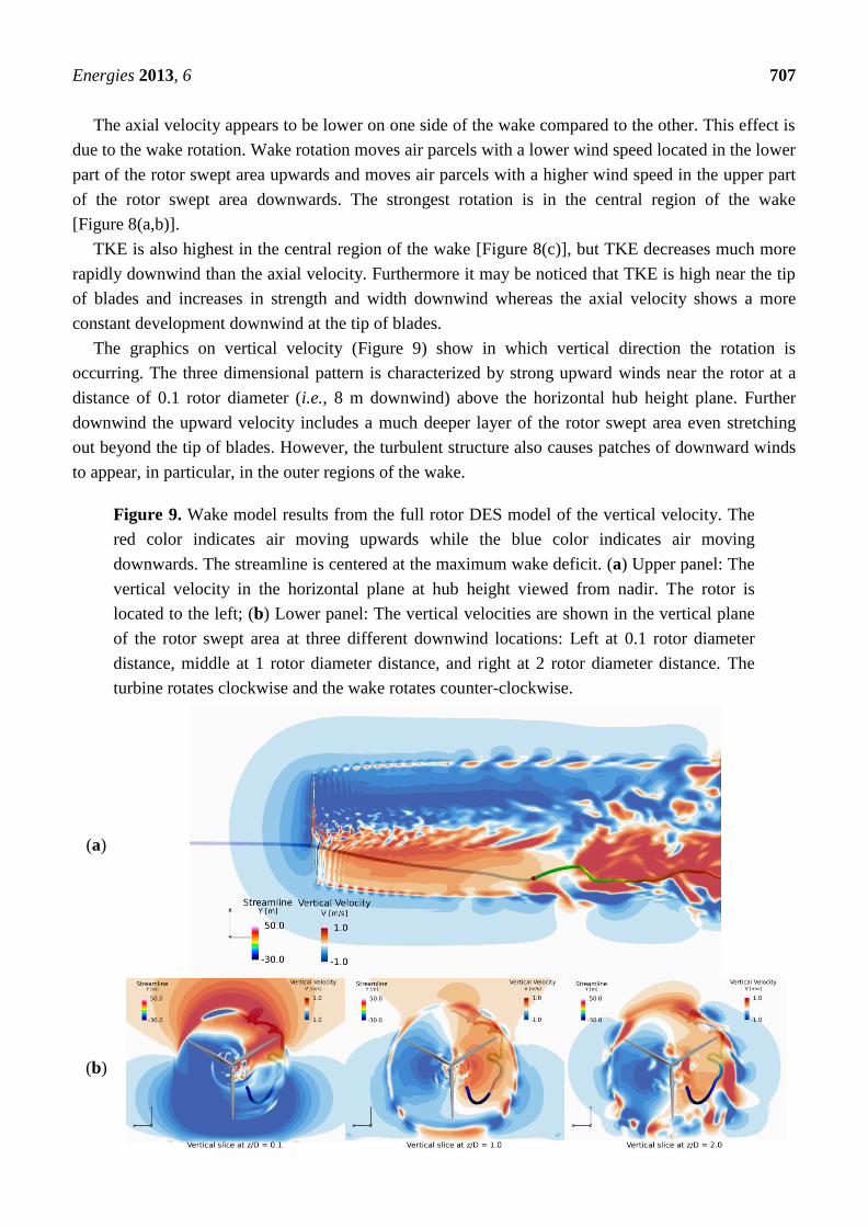
Figure 8. Wake development model results using Detached Eddy Simulation of a full rotor
simulation in laminar inflow. The axial velocity and turbulent kinetic energy (TKE) are
shown using a transparent color count in the plane. The streamline is centered at the
maximum wake deficit and shows that the flow is following the wake rotation, bringing up
air with lower velocities. (a) Upper panel: The axial velocity in the horizontal plane at hub
height viewed in slant range from above; (b) Middle panel: The axial velocity in the
horizontal plane at hub height viewed from nadir; (c) Lower panel: TKE in m2 s
−2 viewed
as in (b). The rotor is located to the left. The turbine rotates clockwise and the wake
rotates counter-clockwise.
(a)
(b)
(c)
Page 12
Energies 2013, 6 707
The axial velocity appears to be lower on one side of the wake compared to the other. This effect is
due to the wake rotation. Wake rotation moves air parcels with a lower wind speed located in the lower
part of the rotor swept area upwards and moves air parcels with a higher wind speed in the upper part
of the rotor swept area downwards. The strongest rotation is in the central region of the wake
[Figure 8(a,b)].
TKE is also highest in the central region of the wake [Figure 8(c)], but TKE decreases much more
rapidly downwind than the axial velocity. Furthermore it may be noticed that TKE is high near the tip
of blades and increases in strength and width downwind whereas the axial velocity shows a more
constant development downwind at the tip of blades.
The graphics on vertical velocity (Figure 9) show in which vertical direction the rotation is
occurring. The three dimensional pattern is characterized by strong upward winds near the rotor at a
distance of 0.1 rotor diameter (i.e., 8 m downwind) above the horizontal hub height plane. Further
downwind the upward velocity includes a much deeper layer of the rotor swept area even stretching
out beyond the tip of blades. However, the turbulent structure also causes patches of downward winds
to appear, in particular, in the outer regions of the wake.
Figure 9. Wake model results from the full rotor DES model of the vertical velocity. The
red color indicates air moving upwards while the blue color indicates air moving
downwards. The streamline is centered at the maximum wake deficit. (a) Upper panel: The
vertical velocity in the horizontal plane at hub height viewed from nadir. The rotor is
located to the left; (b) Lower panel: The vertical velocities are shown in the vertical plane
of the rotor swept area at three different downwind locations: Left at 0.1 rotor diameter
distance, middle at 1 rotor diameter distance, and right at 2 rotor diameter distance. The
turbine rotates clockwise and the wake rotates counter-clockwise.
(a)
(b)
Page 13
Energies 2013, 6 708
At the distance of 1 rotor diameter (80 m) there is a near perfect symmetry with upward winds at
the one side and downward winds at the other side with a gradual decrease in magnitude in winds from
the centre of the hub towards the tip of blades. At the distance of two rotor diameters (160 m) the
turbulence clearly erodes this symmetry and redistributes the air parcels to a more complex structure.
The turbulent imprint to this large-scale wake structure is more pronounced further downwind.
The pressure drop in the wake from the DES simulation is found to have its maximum value very
close to the rotor. The pressure increases downwind with the relatively lowest pressure remaining at
hub height behind the nacelle but at a distance of 1 rotor diameter the pressure depression is modest.
The pressure drop near the tip of blades is localized and the pressure quickly increases downwind
(not shown).
In the wind turbine control regime below rated wind speed both the NM80 pitch controlled turbine
and the Vestas V80 pitch controlled turbine at the Horns Rev 1 wind farm, would typically have a
constant tip speed ratio (velocity of the tip of the blade divided by the incoming wind speed).
Furthermore, for wind speeds lower than or equal to 8 ms−1
the thrust coefficient is nearly constant. It
means that the wake deficit ratio will also be equivalent for velocities lower than 8 ms−1
. These two
parameters combined give us confidence that the state of the wake of the NM80 wind turbine
simulated at 8 ms−1
is of similar nature as the wake of the V80 wind turbine at 4 ms−1
.
5. Wind Farm Wake: Observations
The SCADA data from the Horns Rev 1 wind farm is used to identify the most likely time of the
photographs during the morning of 12 February 2008. The sun angle appears to be slightly before noon
as seen on the sunlight on the fog. It is noted in Figure 2a that one wind turbine (“88”, see Figure 10)
in the southern row was not operating. The SCADA information reveals that this turbine
“started/stopped” (a status where the wind turbine starts and stops one or more times within a period)
in the interval between 10:00 UTC and 10:10 UTC and had this status during the following
50 min. In addition, checking the status of all other turbines in this 50 min time interval allowed the
identification. For the first 10-min time interval only, all other turbines in the southern row were
operating. SCADA information from turbine “48” is missing throughout. Figure 10 shows the status of
all turbines at the relevant 10-min interval. The wind direction of 180.8° observed at M6 at 68 m
confirms the wind direction near hub-height of all turbines in the southern row.
The wind speed observed at M6 at 70 m is 3.64 ms−1
. This is lower than the nacelle wind speed at
all turbines in the southern row that all experience free stream velocity [see Figure 11(a)]. The nacelle
wind speeds in this row show a clear decrease from west to east and the low winds observed at M6
supports this general trend. In Figure 11(a) it is clear that winds at turbines located north of “rotor
stopped” turbines are relatively higher.
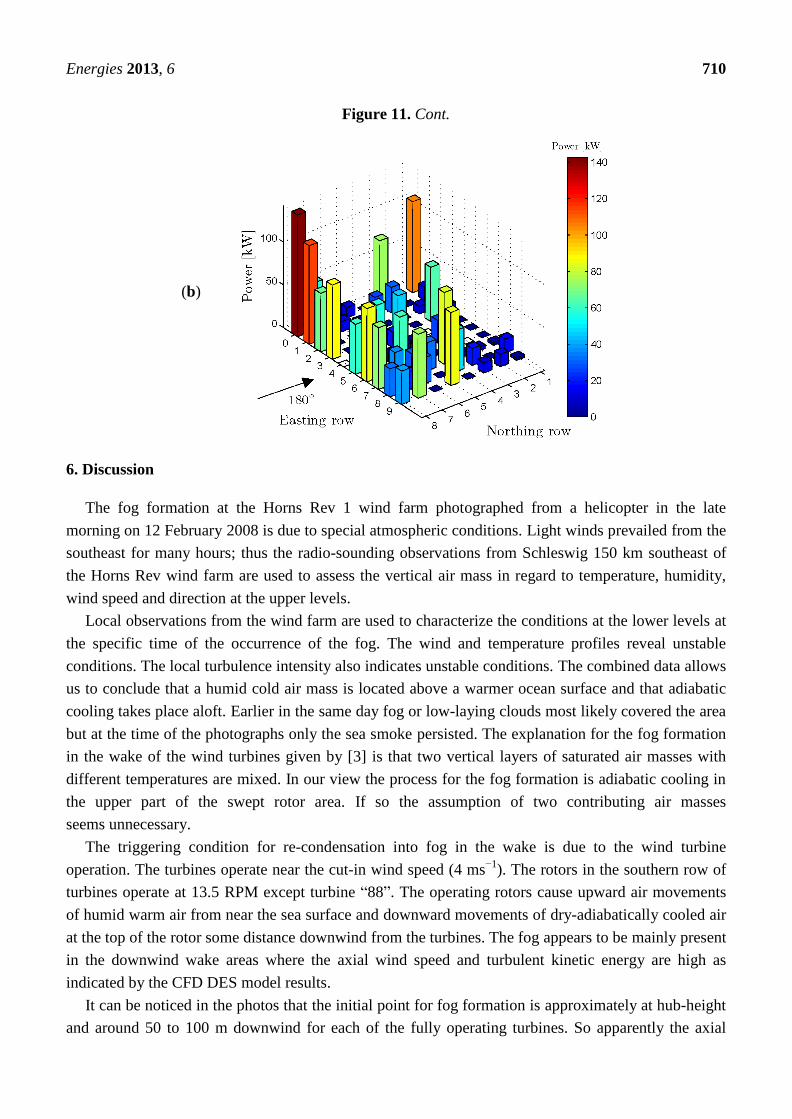
The turbines with relatively high production are those in the first row and turbines located
downwind of stopped turbines [Figure 11(b)]. Compared to the rated power of 2 MW, the amount of
power of the turbines producing the highest, up to 140 kW, is very low. All turbines in the southern
row operated at 13.5 revolutions per minute (RPM) except turbine “88” that was slowing down. No
SCADA data on turbine “48” is available but seen from the photographs this wind turbine did operate.
Page 14
Energies 2013, 6 709
In contrast, most other turbines in the wind farm operated slower. Selected SCADA data are listed in
the Appendix.
Figure 10. The Horns Rev 1 wind turbine layout with numbering and color identification
for operating status at 10:10 UTC on 12 February 2008: Green: operating; Pale blue:
start/stop; Red: rotor stopped; Magenta: faulty scan or power down-regulated; Dark blue:
no SCADA information. The position of the meteorological mast M6 is also indicated. The
first digit in the number indicates the west-east row and the second number indicates the
north-south row. Data are from DONG Energy and Vattenfall.
Figure 11. The Horns Rev 1 data from 12 February 2008 at 10:10 UTC from SCADA data.
(a) Upper panel: Nacelle wind speeds; (b) Lower panel: Measured power. Data are from
DONG Energy and Vattenfall.
(a)
Page 15
Energies 2013, 6 710
Figure 11. Cont.
(b)
6. Discussion
The fog formation at the Horns Rev 1 wind farm photographed from a helicopter in the late
morning on 12 February 2008 is due to special atmospheric conditions. Light winds prevailed from the
southeast for many hours; thus the radio-sounding observations from Schleswig 150 km southeast of
the Horns Rev wind farm are used to assess the vertical air mass in regard to temperature, humidity,
wind speed and direction at the upper levels.
Local observations from the wind farm are used to characterize the conditions at the lower levels at
the specific time of the occurrence of the fog. The wind and temperature profiles reveal unstable
conditions. The local turbulence intensity also indicates unstable conditions. The combined data allows
us to conclude that a humid cold air mass is located above a warmer ocean surface and that adiabatic
cooling takes place aloft. Earlier in the same day fog or low-laying clouds most likely covered the area
but at the time of the photographs only the sea smoke persisted. The explanation for the fog formation
in the wake of the wind turbines given by [3] is that two vertical layers of saturated air masses with
different temperatures are mixed. In our view the process for the fog formation is adiabatic cooling in
the upper part of the swept rotor area. If so the assumption of two contributing air masses
seems unnecessary.
The triggering condition for re-condensation into fog in the wake is due to the wind turbine
operation. The turbines operate near the cut-in wind speed (4 ms−1
). The rotors in the southern row of
turbines operate at 13.5 RPM except turbine “88”. The operating rotors cause upward air movements
of humid warm air from near the sea surface and downward movements of dry-adiabatically cooled air
at the top of the rotor some distance downwind from the turbines. The fog appears to be mainly present
in the downwind wake areas where the axial wind speed and turbulent kinetic energy are high as
indicated by the CFD DES model results.
It can be noticed in the photos that the initial point for fog formation is approximately at hub-height
and around 50 to 100 m downwind for each of the fully operating turbines. So apparently the axial
Page 16
Energies 2013, 6 711
rotation of winds needs to take place through a certain period of time (~22 s) before water droplets
(fog) starts to form from the super-saturated water vapor enhanced by the rotating winds. The initial
condensation seems to occur in the counter-rotating swirl generated by the rotor. In other words, the
induced velocities perpendicular to the wind direction are largest at the root section of the blade and
this means the flow is rotating most here. The counter-clockwise swirl is lifting up warm humid air
from the lower parts of the rotor to a higher level, where it is cooled down and condensation is
accelerated. There is also a pressure drop in this region but of rather low intensity so the turbulent
mixing is probably the most important factor.
The area with fog expands downstream as the individual wakes spread in the vertical and
transversal directions and the neighboring bands of fog blend at a distance of around 2 km downwind.
According to [12] the power deficit at Horns Rev 1 is found to be maximum at the range of wind
speeds 3–5 ms−1
and the wake expansion is large (29°).
In [3] the fog structure is explained from the unstable temperature stratification of the air leading to
the slightly bumpy nature of the wake clouds. In contrast, we find that the large-scale structure of the
fog has a clear imprint from the wake flow dynamics with rotational spiraling bands. This is based on
the axial velocities and turbulent kinetic energy development downwind from the CFD DES wake
model results.
The SCADA data from Horns Rev 1 is used to identify the most likely time of the photographs.
Furthermore, the SCADA data shows the production is low as the wind speed is near cut-in. The
meteorological observation of wind speed at M6 is even lower. It has previously been documented that
coastal wind speed gradients are found near Horns Rev using satellite synthetic aperture radar (SAR)
wind maps and modeling [13]. Also in [14] and [15] satellite and airborne SAR wind observations
showed wind speed gradients locally in and near the Horns Rev 1 wind farm.
The Horns Rev 1 wind farm wake has previously been modeled successfully with wake engineering
models in the wind speed ranges 8 ± 0.5 ms−1
[16] and down to 6 ms−1
[17]. The thrust coefficient is
high in low winds [12] and the resulting wake-disturbed wind speeds are sufficiently low to stop the
downstream turbines. As the wake meanders downwind the start/stop phase of the turbines might
happen several times during the 10-min period. This dynamical effect is pretty difficult to model.
The wake engineering models assume a constant wind speed over 10 min. Thus an engineering
wake model cannot capture neither the wind speed gradient, nor the dynamical changes of meandering
wakes. Furthermore, for a wind speed of 4 ms−1
it will take around 15 min for the flow to pass the
entire wind farm. The PARK model [18] was run for the present case (the results are not shown) and
the agreement with the produced power was not so good. The engineering wake models are calibrated
for higher wind speeds where most wind farm power production takes place. This very special wake
case may possibly be modeled in the future including stability effect. SCADA data for comparison to
future model results are listed in the appendix.
The photographs of the fog formation in the wake of the Horns Rev 1 wind farm are often shown at
wind energy events. It is recommended to be cautious on the interpretation of this wake as it is in fact
not a typical wind farm wake situation at all. Only few turbines within the wind farm operated
normally. The wind speed was so low that only the wind turbines in the front (southern) row except
turbine “88” rotated at 13.5 RPM. Turbine „88‟ and most other turbines in the wind farm operated at
Page 17
Energies 2013, 6 712
less RPM. The fog is most likely caused mainly by the accelerated condensation in the counter-rotating
wake swirl generated by the turbines in the front row.
7. Conclusions
The case of fog formation at the Horns Rev 1 wind farm that occurred 12 February 2008 at 10:10
UTC and was photographed from a helicopter is examined. The special atmospheric conditions are
characterized by a layer of cold humid supersaturated air that re-condensates to fog in the wake of the
turbines. The process is fed by humid warm air up-drafted from below and adiabatic cooled air
down-drafted from above by the counter-rotating swirl generated by the rotors. The wind speed is near
cut-in and most turbines produce very little power. The condensation appears to take place primarily in
the wake regions with relatively high axial wind speed and high turbulent kinetic energy. The
large-scale structure of the fog has an imprint of rotational spiraling bands similar to wake flow
characteristics deduced from CFD DES modeling.
Acknowledgments
We acknowledge the kind permission from Vattenfall to publish the photographs and wind farm
data from DONG Energy and Vattenfall. Furthermore, we acknowledge the sea surface temperature
map from the Danish Meteorological Institute, the wind vector map based on ASCAT from KNMI
produced by the EUMETSAT OSI SAF and the MODIS satellite map from NERC Satellite Receiving
Station, Dundee University, Scotland. We acknowledge the radio-sounding graph from University of
Wyoming. Funding from the EERA DTOC contract FP7-ENERGY-2011/n° 282797 is acknowledged.
We are thankful for the constructive comments from the reviewers.
Appendix
This appendix lists the satellite, radio-sounding and model data (Table A1), observations from the
offshore meteorological mast M6 (Table A2) and SCADA data from Horns Rev 1 (Table A3).
Table A1. Data from satellite, radio-sounding and ocean model for the Horns Rev 1 wind
farm from 12 February 2008. Wind speed (U), relative humidity (RH), temperature (T),
dew-point temperature (Tdew), wind direction (Dir) and pressure (P).
Type of data Time in
UTC Key data Source
SST gridded (AATSR, AVHRR,
MODIS, SEVIRI, AMSR-E)
00:00 At sea surface: 5 °C DMI
Radiosounding Schleswig 00:00 At 48 m: P 1032 hPa, RH 100%, T 3.0 °C,
Tdew 3.0 °C, U 2 ms−1
, Dir 120°
University of
Wyoming
QuikSCAT 05:00 At 10 m: U 3 to 5 ms−1
, Dir 180° NASA
Ocean model 09:00 At 4 m depth: 5 °C DMI
ASCAT 09:16 At 10 m: U 5 ms−1
, Dir 180° KNMI/OSI SAF
Terra MODIS 10:07 Cloud cover NASA
NOAA AVHRR 11:43 Cloud cover NOAA
Page 18
Energies 2013, 6 713
Table A1. Cont.
Type of data Time in
UTC Key data Source
Aqua MODIS 11:50 Cloud cover NASA
Meteosat 12:00 Cloud cover EUMETSAT
Radiosounding Schleswig 12:00 At 48 m: P 1032 hPa, RH 87%, T 3.0 °C,
Tdew 1.0 °C, U 2 ms−1
, Dir 130°
University of
Wyoming
QuikSCAT 18:45 At 10 m: U 3 to 5 ms−1
, Dir 180° NASA
ASCAT 20:45 At 10 m: U 5 ms−1
, Dir 180° KNMI/OSI SAF
Table A2. Meteorological observations are from M6 from 12 February 2008 observed at
various heights at three 10-min periods; before, at and after the wake photos. Pressure (P),
wind speed (U), wind direction (Dir), temperature (T) and turbulence intensity (TI). Data
are from DONG Energy and Vattenfall.
Parameter P U U U Dir Dir T T T TI TI TI
Unit hPa ms−1
ms−1
ms−1
° ° °C °C °C % % %
Height (m) 16 70 40 30 68 28 64 16 −3 70 40 30
10:00 UTC 1037 3.96 3.88 3.75 175.1 184.4 3.6 4.0 4.7 11.16 11.51 15.17
10:10 UTC 1037 3.64 3.57 3.44 180.8 191.0 3.6 4.0 4.7 17.19 15.56 17.76
10:20 UTC 1037 3.89 3.82 3.63 189.0 188.9 3.6 4.0 4.7 10.38 10.38 15.18
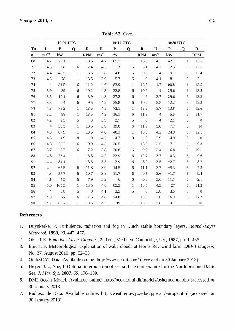
Table A3. The SCADA data from Horns Rev 1 are listed for each turbine (Tu) with the
number as in Figure 10 for three 10-minutes periods; before, at and after the wake photos.
The table contains data on nacelle wind speed (U), produced power (P), rotational speed
(R), and quality flag (Q) for the production data with 1 “Measurement valid”, 5 “Rotor
stopped”, 6 “Start or stop sequence”, 8 “Power is downregulated by centralized control”,
9 “Faulty scan”. Data are from DONG Energy and Vattenfall.
10:00 UTC 10:10 UTC 10:20 UTC
Tu U P Q R U P Q R U P Q R
# ms−1
kW - RPM ms−1
kW - RPM ms−1
kW - RPM
1 5 141.8 1 13.5 4.9 106.4 1 13.5 3.7 34.3 1 13.5
2 5.1 −4.1 5 0 4.4 −4.1 5 0 3.9 −3.7 5 0
3 5.9 213.9 1 13.6 4.7 75.4 1 13.5 4.1 26.8 6 12
4 5.9 −2.2 5 0 4.2 −2.4 5 0 4.4 −2.2 5 0
5 6.1 198.9 1 13.6 3.7 12.1 6 9.6 4.2 17.2 6 6.7
6 5.6 171.6 1 13.5 3.8 34.2 1 13.5 3.7 0.8 6 7.6
7 5.2 158.9 1 13.5 4.3 55.7 1 13.5 3.7 7.9 6 11.5
8 6 184.4 1 13.5 5.7 142.5 1 13.5 5.2 87.9 1 13.5
11 4.7 88.4 6 11.4 3.8 15.5 6 12.1 4.1 29 6 12.4
12 4.7 60.1 6 12.1 3.8 −0.5 6 8.4 3.9 6.6 6 8.8
13 4.8 95.1 1 13.5 3.8 29.7 6 12.5 3.5 11.4 6 11.1
14 5.2 114.1 1 13.5 3.9 25.3 6 12.4 3.8 18.3 6 10.2
15 5.3 137.3 1 13.5 3.5 4.1 6 11.7 3.5 −2.1 6 9.1
Page 19
Energies 2013, 6 714
Table A3. Cont.
10:00 UTC 10:10 UTC 10:20 UTC
Tu U P Q R U P Q R U P Q R
# ms−1
kW - RPM ms−1
kW - RPM ms−1
kW - RPM
16 5.3 117.8 1 13.5 3.6 11.9 6 10.9 3.7 18.9 6 12.4
17 5.3 135.8 1 13.5 3.9 12.4 6 10.6 3.8 −4.8 6 8
18 6 168.3 1 13.5 5.5 115.2 1 13.5 5.2 81.5 1 13.5
21 4.9 99.1 1 13.5 3.8 14 6 12.1 3.5 3.9 6 11.9
22 4.7 103.2 1 13.5 3.5 9.2 6 12.4 3.8 14 6 10.7
23 4.6 92.3 1 13.5 3.5 −5.5 6 10.4 3.9 14.1 6 9.3
24 4.3 76.3 1 13.5 3.6 −6.4 6 2.5 3.8 3 6 5
25 4.8 84 1 13.5 3.8 −11.6 6 5.1 3.9 −1.8 6 8
26 4.3 56.1 1 13.5 3.6 −5.5 6 6.8 3.8 39.3 1 13.5
27 4 18.4 6 12.7 3.3 −0.7 6 9.3 3.6 −8.5 6 2.2
28 5.4 130.1 1 13.5 4.8 68.5 1 13.5 4.8 74.5 1 13.5
31 4.7 70.6 1 13.5 4 12.1 6 9.6 3.9 4.6 6 8.2
32 5.2 135.4 1 13.5 4.4 63.4 1 13.5 4 27.4 6 8.3
33 4.7 −3.1 5 0 3.9 −3.2 5 0 4.2 −2.9 5 0
34 5.1 125.7 1 13.5 3.7 44.9 6 10.7 4 28.3 6 7.5
35 4.6 −6.4 6 1.5 3.4 −6.7 6 6.2 4.1 −5.2 6 3.5
36 4.4 65.5 1 13.5 3.7 19.8 1 13.5 3.6 2.6 6 9.1
37 4.2 34.4 6 10.2 3.9 −6.3 6 2.3 3.6 1.8 6 10
38 5.3 117 1 13.5 5 86.9 1 13.5 4.7 63.1 1 13.5
41 4.7 110.7 1 13.5 3.2 −7.2 6 9.6 3.5 3 6 9.3
42 5.3 124.1 1 13.5 3.8 2.5 6 11.4 4.2 20.1 6 9.9
43 Na Na Na Na Na Na Na Na Na Na Na Na
44 4.2 60.8 1 13.5 3.6 −11.6 6 5.3 4.1 37.4 6 9.6
45 4.5 64 1 13.5 4 18.3 6 9.1 4.1 19.7 6 9.8
46 5.2 113.2 1 13.5 4.4 57.3 1 13.5 4.4 51.5 1 13.5
47 5.2 −20.6 9 0 4.9 −20.5 9 0 4.8 −14.8 5 0
48 Na Na Na Na Na Na Na Na Na Na Na Na
51 4.7 −2.6 5 0 3.8 −2.9 5 0 4.7 −2.7 5 0
52 4.8 79.4 1 13.5 3.9 9.8 6 12.4 5 77.2 1 13.5
53 5.4 126.3 1 13.5 4 26.3 6 11.6 4.5 49.7 6 11.1
54 4.7 −5.5 5 0 4 −5.9 5 0 4.7 −5.4 5 0
55 4.2 27 6 12.5 3.9 11.7 6 11.1 4 19.5 6 12.5
56 4.2 67.8 1 13.5 3.3 9.1 6 12.3 3.4 13.8 6 12.4
57 3.7 25.1 6 12.3 3.2 −9.7 6 5.3 3.4 6.4 6 9.3
58 5.3 95 1 13.5 4.8 58.5 1 13.5 4.6 37.9 1 13.5
61 5.4 137.4 1 13.5 3.6 −4.8 6 11.8 4.3 30.1 6 11.6
62 Na Na Na Na Na Na Na Na Na Na Na Na
63 4.8 109.5 1 13.5 4.1 13.3 6 10.9 4.1 42.4 1 13.5
64 4.2 59.7 6 11.2 4 1.8 6 5.1 3.8 −5.6 6 6.6
65 4 54.9 1 13.5 4 19.3 6 8 4.1 49.3 1 13.5
66 4.9 79.8 1 13.5 4.8 61 1 13.5 4.4 39.6 1 13.5
67 4.2 −3.5 5 0 4.5 −3.4 5 0 3.8 −3.2 5 0
Page 20
Energies 2013, 6 715
Table A3. Cont.
10:00 UTC 10:10 UTC 10:20 UTC
Tu U P Q R U P Q R U P Q R
# ms−1
kW - RPM ms−1
kW - RPM ms−1
kW - RPM
68 4.7 77.1 1 13.5 4.7 85.7 1 13.5 4.2 42.7 1 13.5
71 4.3 7.8 6 12.4 4.5 3 6 5.1 4.3 12.3 6 12.5
72 4.4 49.5 1 13.5 3.8 4.6 6 9.8 4 19.1 6 12.4
73 4.3 78 1 13.5 3.9 5.7 6 9 4.1 −8.1 6 3.1
74 4 31.5 6 11.2 4.6 83.9 1 13.5 4.7 100.8 1 13.5
75 3.9 39 6 10.2 4.3 32.8 6 10.6 4 25.6 1 13.5
76 3.5 10.1 6 8.9 4.3 27.2 6 9 3.7 29.6 6 13.3
77 3.3 0.4 6 9.5 4.2 35.8 6 10.2 3.5 12.2 6 12.3
78 4.8 79.2 1 13.5 4.5 72.1 1 13.5 3.7 13.8 6 12.6
81 5.2 98 1 13.5 4.3 16.1 6 11.3 4 5.5 6 11.7
82 4.2 −2.5 5 0 3.9 −2.7 5 0 4 −2.1 5 0
83 4 38.3 1 13.5 3.9 19.8 6 11.9 3.8 7.7 6 10
84 4.8 67.9 1 13.5 4.6 48.3 1 13.5 4.2 24.9 6 12.1
85 4.5 −4.9 8 0 4.3 −4.7 8 0 3.9 −4.9 8 0
86 4.3 25.7 6 10.9 4.3 30.5 1 13.5 3.5 −7.1 6 6.3
87 3.7 −5.7 6 7.2 3.8 20.8 6 9.9 3.4 16.8 6 10.1
88 4.8 73.4 1 13.5 4.2 32.9 6 12.7 3.7 10.3 6 9.6
91 4.4 84.1 1 13.5 3.5 2.9 6 8.9 3.5 −2.7 6 8.7
92 4.2 67.5 6 11.8 3.9 14.5 6 11.1 3.7 −5.3 6 7.3
93 4.3 57.7 6 10.7 3.8 11.7 6 9.5 3.6 −1.7 6 9.4
94 4.1 4.5 6 7.9 3.9 −6 6 6.8 3.6 −11.1 6 2.1
95 5.6 165.3 1 13.5 4.8 85.5 1 13.5 4.3 27 6 11.3
96 4 −3.8 5 0 4.1 −3.5 5 0 3.8 −3.5 5 0
97 4.8 72 6 11.6 4.6 74.8 1 13.5 3.8 16.3 6 12.2
98 4.7 66.2 1 13.5 4.3 39 1 13.5 3.6 4.1 6 10
References
1. Duynkerke, P. Turbulence, radiation and fog in Dutch stable boundary layers. Bound.-Layer
Meteorol. 1998, 90, 447–477.
2. Oke, T.R. Boundary Layer Climates, 2nd ed.; Methuen: Cambridge, UK, 1987; pp. 1–435.
3. Emeis, S. Meteorological explanation of wake clouds at Horns Rev wind farm. DEWI Magazin,
No. 37, August 2010, pp. 52–55.
4. QuikSCAT Data. Available online: http://www.ssmi.com/ (accessed on 30 January 2013).
5. Høyer, J.L.; She, J. Optimal interpolation of sea surface temperature for the North Sea and Baltic
Sea. J. Mar. Sys. 2007, 65, 176–189.
6. DMI Ocean Model. Available online: http://ocean.dmi.dk/models/bshcmod.uk.php (accessed on
30 January 2013).
7. Radiosonde Data. Available online: http://weather.uwyo.edu/upperair/europe.html (accessed on
30 January 2013).
Page 21
Energies 2013, 6 716
8. Radiosonde Data. Available online: http://www.esbjerg-lufthavn.dk/uk/general/airport-data.html
(accessed on 30 January 2013).
9. Meteorological Data. Available online: http://en.windfinder.com/forecast/list_sylt (accessed on 30
January 2013).
10. Peña, A.; Hasager, C.B.; Gryning, S.E.; Courtney, M.; Antoniou, I.; Mikkelsen, T. Offshore wind
profiling using light detection and ranging measurements. Wind Energy 2009, 12, 105–124.
11. Troldborg, N.; Zahle, F.; Réthoré, P.-E.; Sørensen, N.N. Comparison fo the Wake of Different
Types of Wind Turbine CFD Models; American Institute of Aeronautics and Astronautics
(AIAA): Nashville, TN, USA, 2012.
12. Hansen, K.; Barthelmie, R.J.; Jensen, L.E.; Sommer, A. The impact of turbulence intensity and
atmospheric stability on power deficits due to wind turbine wakes at Horns Rev wind farm.
Wind Energy 2012, 15, 183–196.
13. Barthelmie, R.; Badger, J.; Pryor, S.; Hasager, C.B.; Christiansen, M.B.; Jørgensen, B.H. Offshore
coastal wind speed gradients: Issues for the design and development of large offshore windfarms.
Wind Eng. 2007, 31, 369–382.
14. Christiansen, M.B.; Hasager, C.B. Using airborne and satellite SAR for wake mapping offshore.
Wind Energy 2006, 9, 437–455.
15. Christiansen, M.B.; Hasager, C.B. Wake effects of large offshore wind farms identified from
satellite SAR. Remote Sens. Environ. 2005, 98, 251–268.
16. Barthelmie, R.; Hansen, K.; Frandsen, S.; Rathmann, O.; Schepers, G.; Schlez, W.; Phillips, J.;
Rados, K.; Zervos, A.; Politis, E.; et al. Modelling and measuring flow and wind turbine wakes in
large wind farms offshore. Wind Energy 2009, 12, 431–444.
17. Barthelmie, R.J.; Pryor, S.C.; Frandsen, S.; Hansen, K.; Schepers, G.; Rados, K.; Schlez, W.;
Neubert, A.; Jensen, L.E.; Neckelmann, S. Quantifying the impact of wind turbine wakes on
power output at offfshore wind farms. J. Atmos. Ocean. Technol. 2010, 27, 1302–1317.
18. Katic, C.; Jensen, N.O. A Simple Model for Cluster Efficiency. In Proceedings of European Wind
Energy Association Conference and Exhibition, Rome, Italy, 7–9 October 1986.
© 2013 by the authors; licensee MDPI, Basel, Switzerland. This article is an open access article
distributed under the terms and conditions of the Creative Commons Attribution license
(http://creativecommons.org/licenses/by/3.0/).