Work Performed Under Contract No. AM04-80AL 13137 May 1, 1984 LANGLEY RESEARCH CENTER LIBRARY. NASA HAMPTON, VIRGINIA liBRARY DOE/ JPL-1 060·66 (DE85000337) NASA-CR-173896 19840024844 By E. J. Roschke Jet Propulsion Laboratory Pasadena, California WIND LOADING ON SOLAR CONCENTRATORS: SOME GENERAL CONSIDERATIONS Technical Information Center Office of Scientific and Technical Information United States Department of Energy https://ntrs.nasa.gov/search.jsp?R=19840024844 2020-04-18T09:52:50+00:00Z
Transcript
Work Performed Under Contract No. AM04-80AL13137
May 1, 1984
LANGLEY RESEARCH CENTERLIBRARY. NASA
HAMPTON, VIRGINIA
liBRARY C~py
DOE/JPL-1 060·66(DE85000337)
NASA-CR-17389619840024844
ByE. J. Roschke
Jet Propulsion LaboratoryPasadena, California
WIND LOADING ON SOLAR CONCENTRATORS:SOME GENERAL CONSIDERATIONS
This report was prepared as an account of work sponsored by an agency of theUnited States Government. Neither the United States Government nor any agencythereof, nor any of their employees, makes any warranty, express or implied, orassumes any legal liability or responsibility for the accuracy, completeness, or usefulness of any information, apparatus, product, or process disclosed, or representsthat its use would not infringe privately owned rights. Reference herein to any specific commercial product, process, or service by trade name, trademark, manufacturer, or otherwise does not necessarily constitute or imply its endorsement, recommendation, or favoring by the United States Government or any agency thereof.The views and opinions of authors expressed herein do not necessarily state orreflect those of the United States Government or any agency thereof.
This report has been reproduced directly from the best available copy.
Available from the National Technical Information Service, U. S. Department ofCommerce, Springfield, Virginia 22161.
Price: Printed Copy A08Microfiche AOI
Codes are used for pricing all publications. The code is determined by the numberof pages in the publication. Information pertaining to the pricing codes can befound in the current issues of the following publications, which are generally available in most libraries: Energy Research Abstracts (ERA); Government ReportsAnnouncements and Index (GRA and I); Scientific and Technical AbstractReports (STAR); and publication NTIS-PR-360 available from NTIS at the aboveaddress.
(:ORP= -.Jet Pr·,)p!.jl :31 Of~! Lat):! (=a I l forril a Ir!st~ /of Tecf-!~ ~ Pasader!a:SAP: He A08/MF· AOI
A8S: A survey was completed. to examlne the problems and complications arisingfr·orH 1}.1in(~ loadit19 orr sc~lar conc:erltfA ator:3: tlJlnd lC12cfiri9 i::3 site :3pec~ltl(::
and has an lffiPortant bearln9 on the design, cost, performance! operationand maintenance~ safety! survival-, ~nd replacement of solar collectjngsYstems: Emphasis herein is on paraboloidal, two-axis tracking sYstems:Thermal ·rece1ver problems a~so are discussed: Wind characteristics arediscussed from a general point of vi.ew: Current methods for determining·design wind speed are revlewed: Aerodynamic Goe f1cients are defined a0ui ll\lstrative e~a:arnpl-es are p~'''eser!te(~: t~jir!c! t\lt1r~e testir19 is (~lS(:!..J:3:3ed! ar~c~·
5105·130
Solar Thermal Power Systems ProjectParabolic Dish Systems Development
DOE/JPL-1 060-66(J PL·Pub-83-1 01)(OE85000337)
Distribution Category UC·62b
Wind Loading onSolar Concentrators:Some General Considerations
E.J. Raschke
May 1,1984
Prepared for
U.S. Department of Energy
Through an Agreement withNational Aeronautics and Space Administration
by
Jet Propulsion LaboratoryCalifornia Institute of TechnologyPasadena, California
JPL Publication 83·101
ABSTRACT
A survey has been completed to examine the problems and complicationsarising from wind loading on solar concentrators. Wind loading is sitespecific and has an important bearing on the design, cost, performance,operation and maintenance, safety, survival, and replacement of solarcollecting systems. Emphasis herein is on paraboloidal, two-axis trackingsystems. Thermal receiver problems also are discussed.
Wind characteristics are discussed from a general point of view; currentmethods for determining design wind speed are reviewed. Aerodynamiccoefficients are defined and illustrative examples are presented. Wind tunneltesting is discussed,and environmental wind tunnels are reviewed; recentresults on heliostat arrays are reviewed as well. Aeroelasticity in relationto structural design is discussed briefly.
Wind loads, i.e., forces and moments, are proportional to the square ofthe mean wind velocity. Forces are proportional to the square of concentratordiameter, and moments are proportional to the cube of diameter. Thus, windloads have an important bearing on size selection from both cost and performance standpoints. It is concluded that sufficient information exists so thatreasonably accurate predictions of wind loading are possible for a givenparaboloidal concentrator configuration, provided that reliable and relevantwind conditions are specified. Such predictions will be useful to the designengineer and to the systems engineer as well. Information is lacking, however,on wind effects in field arrays of paraboloidal concentrators. Wind tunneltests have been performed on model heliostat arrays, but there are importantaerodynamic differences between heliostats and paraboloidal dishes.
iii
PMF~E
This report is based on work that was completed at the Jet PropulsionLaboratory (JPL) in July 1980. Subsequently, portions of the unpublishedmemorandum were reviewed internally by M. Alper, L. Jaffe, E. Laumann, R. Levy,W. Menard, J. Patzo1d, R. Turner, and L. Wen. This report has been updated toinclude revisions, corrections, and additional references, tables, and figures.
Liberal use has been made of charts, graphs, and tables obtained (oradapted) from other literature, which results in a mixture of English andmetric units. These differences in units arise from historical usage that hasbecome conventional in the diverse fields of aeronautics and aerodynamics,meteorology, atmospheric physics, and various fields of engineering and science.
ACKNOWLEDGMENTS
Many JPL people prOVided the author with reference sources, the referencesthemselves, useful data and informati~n, and otherwise prOVided support andencouragement: F. Livingston provided information sources relating to pastwind tunnel testing of JPL paraboloidal dish models (Goldstone antenna).B. DaYman kindly provided access to unpublished internal reports (Refs. 13, 70,71, and 92). S. Holian provided Edwards Air Force Base wind data (Ref. 45).H. Bank, L.· Wen, J. Patzo1d, and H. Steele provided useful information ofvarious types. R. Wallace prOVided Ref. 80, and T. Fujita provided Refs. 63and 64.
Special thanks are due to S. Peglow, Sandia National Laboratories Livermore, for providing Ref. 62; and to D. Elliott, U.S. Department of Energy(DOE) San Francisco Operations Office, for providing Refs. 58, 59, and 60.
This report was published by JPL through the National Aeronautics andSpace Administration (NASA) Task Order RE-152, Amendment 327 and was sponsoredby DOE under Interagency Agreement DE-AM04-80AL13137 with NASA.
A. WIND DATA FOR EDWARDS AIR FORCE BASE AND OTHER SOUTHERNCALIFORNIA SITES • • • • • • • • • • • • • • • • • • • • • · . A-I
B. BASIC WIND SPEEDS FOR THE UNITED STATES •••• • • • • • • • B-1
C. APPROXIMATE WIND FORCE RATIOS FOR A SQUARE PLATE • • • • • • • C-l
D. SELECTED WIND TUNNEL RESULTS OF THE MODEL GOLDSTONERADIO ANTENNA •• • • • • • • • • • • • • • • • • • • • • • • 0-1
E. WIND TUNNEL RESULTS OF A FULL-SCALE HELIOSTAT ••• . . . E-l
F. ANALYTICAL RESULTS FOR A SECOND-GENERATION HELIOSTAT •
vii
• • · . F-l
SECTION I
INTRODUCTION
Many fields of engineering and the physical sciences come to bear in thesuccessful design, construction and operation of paraboloidal reflectors,whether they are solar concentrators, radio antennas, or astronomical radio/optical telescopes. They are, to varying degrees, large precision instrumentsthat must perform well even in often hostile environments.
Performance of reflecting surfaces depends essentially on two types offactors: (1) manufacturing and assembly tolerances, and (2) changes broughtabout by environmental conditions. There is no single universally accepteddefinition of surface accuracy, partly because of a disparity between applied,theoretical statistical methods and practical, low-cost measurement techniques.The problem is to relate measurable and quantifiable surface irregularities tooverall optical performance. Surface slope error frequently has been used forcharacterizing the optical performance of solar paraboloidal surfaces, e.g.,see Appendix A of Reference 1.
Environmental factors may stem from climate/weather effects or geolog5.caleffects. Among the former are hail, snow/ice loads, sand/dirt erosion, thermaldifferentials caused by variable heating effects such as partial shading, andwind loads varying from "normal" to those caused by severe local storms such asthunderstorms and tornados; wind loading tends to exacerbate other environmental effects. Included in the latter (geological factors) are Earth settlingand slippage, and earthquakes. Additionally, there are static gravitationalloads that must be addressed during design. Clearly, all of these factors mustbe considered in a cost and performance tradeoff for design, fabrication, andlong-term operation. The utility or degree of expected usage of a solar plantwill singularly affect the tradeoffs.
The present survey is confined mostly to wind loading, which itself isextremely complicated and has far-reaching consequences. Wind loads have adirect influence on the design, cost, optical performance, operation andmaintenance, safety, survival, and replacement of solar concentrators. Thesewill aff ect :
• Dimensional stability of structural reflecting surfaces and supportstructures
• Pointing and tracking accuracy
• Loads on drive mechanisms
• Safety/survival (in high Winds)
• Base/foundation design
• Potential structural vibrations that depend on wind conditions,aerodynamic shape, natural frequency, and structural damping
1-1
Wind loads, i.e., forces, and moments or torques, depend on a large number ofvariables that include:
• Dish configuration, e.g., focal length to diameter ratio (f/D), andporosity of reflecting surfaces
• Dish diameter (concentrator size)
• Wind velocity (speed and direction)
• Wind velocity profile
• Gust (turbulence) magnitude and frequency
• Ground clearance (dish to ground)
• Steering axis position/location
• Design of base, reflecting surface support, and multipod structures
• Field layout (multiple dish systems)
The main purposes of this survey were to review wind loading considerations for paraboloidal solar concentrators and to document useful sourcesof information that are pertinent to the various aspects of wind loading.Information is presented on general wind characteristics, design wind speed,aerodynamic coefficients, wind tunnel testing of models, and aeroelasticityproblems. Results on heliostat field arrays will be discussed as well. Somewind data for Edwards Air Force Base is presented in the Appendixes. Thematerial 1s not intended to be directly applicable for design purposes but,rather, to illustrate descriptive examples. Liberal use has been made ofcharts, graphs, and tables taken (or adapted) from other literature; therefore,an unavoidable mixture of English and metric units is seen.
1-2
SECTION II
BACKGROUND
Rudimentary wind engineering has historic roots dating at least as earlyas the design of windmills, to develop mechanical power, and wind shelters.The development of large urban and industrial centers containing many largeand complex structures required more sophisticated approaches for wind loading design. An early application of modern wind engineering was to suspensionbridges (Ref. 2). Building codes have evolved and are steadily being improvedas the local safety and comfort needs dictate. A large and growing literatureon wind engineering exists; a new periodical, The Journal of IndustrialAerodynamics, is devoted to such diverse applications as wind turbines, smokestacks and cooling towers, high-rise buildings, ground transportation, airpollution problems, and atmospheric physics. Within the last decade specialwind tunnels have been developed and used in model studies for numerousindustrial, environmental, and meteorological applications.
The starting point for this review was the literature relating toterrestrial radio antennas for deep-space communications. Work on large,steerab1e radio antennas began in the late 1950s and continued throughout the19608; a wealth of information is furnished in Ref. 3. The Jet PropulsionLaboratory (JPL) began wind tunnel testing of paraboloidal reflectors duringthe early 1960's; the immediate application of that work was to the largeGoldstone radio antenna at the Goldstone Deep-Space Communication Complex(GnSCC);see Ref. 4. It is interesting that the total cost of the model windtunnel testing for the Goldstone antenna was less than 1% of the total estimatedproject cost (Ref. 5). It is likely that wind tunnel testing costs for modelparaboloidal solar concentrators and field arrays would be an even smallerfraction of the total cost of a solar plant.
There are several recurring themes in the radio antenna wind engineeringliterature. Wind conditions are highly site specific and, therefore, reliablewind measurements as close to the selected site as possible are highly desirable,and records should include as many years of observation as possible. Both"steady" and gust velocities should be known to help determine the design windvelocity as well as various safety factors for design. The cost/performancetradeoff will be strongly influenced by this input information. Clearly, atoo-high design wind velocity will result in an over-designed, costly reflector;but the probability of reduced performance, reduced operating time, and susceptibility to damage will increase with decreasing design velocity. Good windtunnel data should be available for design. Wind tunnel tests on scale modelsshould be performed because they may provide crucial information, and will incuran insignificant relative investment.
Very little wind tunnel information on solar dish concentrators existsfor single models, and none exists for field-array models. Radio antenna data .probably are sufficient for preliminary design purposes, but may not be adequatefor final design or field deployment. Radio antennas differ from solarconcentrators .in many respects. Large radio antennas are larger than solarconcentrators are ever likely to be. They are custom, one-of-a-kind designsthat are not intended for mass production. They are relatively deeper (shorter
2-1
f/D), and have different operating modes; long-term reliability must be higherthan solar concentrators. Finally, they are not used in close-packed arrays.
Although radio antennas are moving (tracking) structures, paraboloidalradio reflectors generally are designed by methods similar to those used forbuildings, i.e., a static design wind velocity is used. However, there aredifferent wind velocity values associated with different performance and safetylevels. Some preliminary wind requirements for the Goldstone antenna areshown in Table 1 as they were set forth in Ref. 5.
A scenario for probability of wind damage is shown in Figure 1 (fromRef. 6), where wind pressure is proportional to the square of wind velocity.Failure modes are converted to the probability of wind damage occurrence inthe lower part of Figure 1. Repair costs mount with increasing wind velocity.Failure (Ref. 6) is defined as structural collapse or permanent deformationsthat affect pointing/tracking accuracy and/or performance. Structural deformations have been widely discussed in the literature (e.g., Refs. 6, 7, and 8).Complete damage or failure necessitates module replacement. In the case of alarge field array, it might be possible to develop different strategies forrepair/replacement using statistical models for local wind conditions andreliability statistics developed for components, modules, and groups of modules.Such studies might affect initial capital costs as well as operation andmaintenance costs.
2-2
SECTION III
WIND CHARACTERISTICS
Wind is caused by atmospheric pressure differences that arise from unequalheating of the Earth's surface. Atmospheric disturbances may vary in size fromvery small (several meters) to almost global proportions. Important factorsthat influence the wind include the Earth's rotation, cloud cover, precipitation,nonuniform surface temperature and roughness, and topographic relief (Ref. 9).It is very difficult to characterize wind mathematically because of its extremevariability and randomness. Useful descriptions -can be formulated by statisticalapproaches, expecially when high-quality, long-term wind measurements existfora specific site of interest. Such work has been in progress for the solarthermal plant planned for the Barstow, California site (Ref. 10). In that case,10 years of data at the Daggett, China Lake, and Edwards Air Force Base weatherstations have been utilized. Parameters in common use include time-average ofwind speed and temperature, recurrence periods for maximum wind speeds, probabilities coupling wind direction at a specified speed, and variations in velocitycomponents (turbulence). All of these parameters may vary with height abovethe Earth's surface. Height variations are discussed subsequently.
A. THE ATMOSPHERIC SURFACE LAYER
The planetary, or atmospheric, boundary layer is loosely described as alayer that has a thickness of roughly 1000 ft, i.e., it extends to an altitude,which varies with many conditions such as surface roughness, of several thousan4 feet. In approximately the upper 90% of this layer, the Earth's rotationand thermal stratification play dominant roles. There may be strong verticalmixing; wind direction varies with altitude and need not be parallel (locally)to the Earth's surface. It is at the upper regions of the planetary boundarylayer that the geostrophic or "free-stream" wind speed is achieved unencumberedby surface friction. This velocity is sometimes called the gradient velocity,and has been expressed (Ref. 11) as:
rw sin xC( pdP/dN + i )1/2 - 1 ]~ rw2 sin2 A
(1)
where r is the radius of curvature of isobars, w is the Earth's rotationalspeed, X is angle of latitude, dP/dN represents the pressure gradient, and Pis the density of air. For example, Equation (1) is useful when precise weatherdata exists.
Figure 2 (from Ref. 9) shows a typical planetary boundary layer model.Conditions for the model are that the atmosphere is horizontally homogeneous,dry, with adiabatic lapse rate, no vertical motions, invariant velocityfluctuations, and negligible effects of turbulence. The lower portion of theplanetary boundary layer is often called the atmospheric surface layer(Figure 2). Its thickness may vary from 100 ft (Ref. 12) to perhaps 500 ftand, for neutrally stable atmospheres, it often is a region of constant stress,momentum, and heat fluxes for moderate to strong winds. The atmospheric surface
3-1
layer may be very thin at night (Ref. 12), when thermal stratification isstrong. Because most man-made structures will be immersed in the atmosphericsurface layer, it is the region of main interest. The Earth's rotation andthermal stratification are not dominant effects for strong wind conditions inthe atmospheric surface layer. Moderate to strong wind conditions are importantfor structure design; conversely, weak wind conditions may be more critical forair-pollution problems.
B. VELOCITY PROFILES AND MODELS
An awareness of wind velocity variation with height above ground isimportant to the wind and design engineers for two reasons: (1) wind loadsvary as the square of time-mean velocity and, therefore, the effects of varyingforces and moments become increasingly important as the size of a structureincreases, and (2) wind tunnel testing of model structures should be conductedusing a boundary layer that closely models an expected atmospheric surfacelayer. The latter point becomes apparent for dish antennas in Figure 3 (fromRef. 13). Note the variation of dynamic pressure across the antenna surfacefor various elevation angles. Note, also, that the unmodified wind tunnelboundary layer would lead to essentially constant (vertically invariant)velocity across the antenna surface.
Various empirical and semi-empirical forms have been developed to expressthe variation of wind velocity with height. These include the spiral, exponential and logarithmic forms. Various logarithmic forms have been developed(e.g., Refs. 12, 14, and 15). Exponential, or power law, forms are morecommonly used for design purposes because of their simplicity and relativelygood accuracy (e.g., Refs. 9,11, and 15). The general power-law expression is:
(2)
where z is height above ground, VG is the gradient wind velocity at the gradientheight zG' and n is the power-law index. Equation (2) is similar to commonboundary layer profiles that occur in fluid dynamics, e.g., n has the value of2 and 7, respectively, for fully developed laminar and turbulent flat-plateboundary layers. A test of the power-law expression for the wind velocityprofile shown in Figure 2 is presented in Figure 4, where individual pointshave been taken from Figure 2. The inverse slope in log-log coordinates is0.35 so that n = 2.86; the fit is good up to a height of approximately 300 m,or about 1000 ft. Equation (2) was found to fit six different sets of airportweather data (measured at either 10 m or 100 m) using a value of n = 6 (Ref. 16).
Both nand zG vary with surface roughness, and zG may vary at the samesite between day and night and the seasons of the year. Surface roughnessdoes not refer to the height of individual structures or obstacles (trees,rocks, etc.) but rather to the statistical average that gives rise to thelocal surface friction. Davenport (Ref. 11) was able to correlate a largeamount of wind data to arrive at a relationship between surface roughness andvalues of nand zG. His results are reproduced here in Table 2 and Figure5. Cermak (Ref. 9) replotted Davenport's data in a form shown here in Figure 6,where lin and zG are plotted as functions of the statistical surface roughnesslength zo. The lower curve for l/n (Figure 6) is based on an empiricalexpression proposed in Ref. 17.
3-2
The reference velocity VG (gradient wind velocity) used in Equation (2),and displayed in Figure 5, is based on relatively few high-altitude measurementsand is difficult to establish. Wind measurements in this country and Europeare becoming standardized at 30 ft and 10 m off the ground, respectively.Airport weather data abounds. Thus, it is convenient to convert'Equation (2)to a reference velocity at 30 ft for flat, open country (i.e., n = 7,zG = 900 ft):
or
where Vz is wind speed at height z, V30 is the reference velocity at 30 ftabove ground, and zG is the gradient wind height (Table 2 or Figure 6).
(3)
Power-law and logarithmic velocity profile models are valid only forneutral or near-neutral atmospheric conditions in flat terrain far removedfrom large topographic features. They apply for relatively slow-changingweather conditions (near-steady state) when changes in the horizontal planeare small. The simplest case of neutral stability occurs when the verticaltemperature distribution follows the adiabatic lapse rate. Thus, these modelsapply for moderate to strong winds and to large-scale mature storms whereturbulence causes thorough mixing without violent thermal interchange; thedominating influence is surface roughness. They do not apply to st~rms withstrong vertical interchanges that destroy the boundary layer structure andare therefore unstable. Examples of unstable storms are severe local thunderstorms, frontal squalls, tornados, and hurricanes. In such storms verticalheat and momentum exhanges are dominant factors, not the surface roughness; infact, the power-law exponent lin may approach zero for such storms. In recentyears much progress has been made in modeling the planetary boundary layer,for both stable and unstable atmospheric conditions (Ref. 18).
Stable atmospheric conditions occur when the temperature increases withheight, i.e., the inversion case. Temperature inversions most often occur atnight when the atmospheric surface layer tends to be the thinnest and thesurface wind speeds are the smallest. However, they may occur during the dayas well. In Figure 7 (from Ref. 19), a low-level jet is revealed by threesmoke plumes issuing from a weather tower at Brookhaven, New York. A hypothetical velocity profile (artist's rendition), divided into three zones, hasbeen superimposed on the photograph. The location of zero velocity, but 'maximum wind shear, appears to be about 75 ft above ground. Low-level jetscan be dangerous to landing aircraft (Ref. 14). Rather large (mesoscale)nocturnal jet winds may occur between inVersion layers and are common in flat,open country (Ref. 20).
For additional information the reader may consult Refs. 9, 11, 12, 14, 15,17, and 18.
3-3
C. GUST CHARACTERISTICS
Gust and turbulence characteristics are important for solar concentratorsinsofar as they contribute to additional wind loads above those based on meanwind speed, cause aerodynamic vibration and amplification, and affect pointingand tracking. Of interest are the magnitude of fluctuating components ofvelocity, their duration or period, the frequency and probability of theiroccurrence, relations or correlations among the various components, and thespat~al size of eddies. This is a specialized and extremely complex field thatcannot be treated in depth in this report; the reader may consult Refs. 9, 15,19, 21, and 22 for more detailed information. Short wind fluctuations thatappear over a period of 1 hour are generally termed gusts (Ref. 22); turbulentfluctuations seem to be associated with even shorter time durations, and usuallyrefer to rapid, random departures from the mean wind speed.
A typical record of horizontal wind speed is shown at three heights aboveground in Figure 8 (from Ref. 22). Note that the wind speed seems to have asteady component with superimposed irregular fluctuations. The steady componentincreases with height but the fluctuating component seems to be relativelyindependent of height, in agreement with one of the conclusions of Ref. 19. Longduration fluctuations seem similar at the different heights, but this is nottrue of short-duration fluctuations. Mean wind speed calculated over periodsof 20 min to 1 hour probably will differ little over various randomly selectedperiods, but mean wind speeds for short periods, such as 1/2 min, will varyconsiderably. Hence, wind speeds averaged over a i-hour duration are bestadapted to determining wind loads except for conditions when weather is changingrapidly.
It is well known that fluctuating fluid components can markedly increasethe forces on a submerged body. Figure 9, for example, shows the increase indrag coefficient in air of a flat plate in fluctuating flow. In Figure 9(from Ref. 22), the abscissa is the dimensionless reduced frequency. In fluidmechanics this is the Strouhal number commonly associated with periodic, orvortex, flows; the symbol n is the frequency of the "periodic·· fluctuationssuperimposed on a mean speed of V. The Strouhal number is, essentially, adimensionless frequency of vortex shedding or wake periodicity. In the exampleshown here, the effective drag coefficient may increase by a factor of 1.5 to1.8 because of fluctuating flow. See Ref. 16 for further examples anddiscussion.
The magnitude of gusts relative to the mean wind speed is of interest fordesign purposes. A typical example of the maximum 3-s gust speed in a givenhour, and the mean speed at a height of 10 m, is shown to be dependent onsurface roughness in Figure lOa (from Ref. 23). The surface roughnessesindicated in Figure lOa are similar to those shown in Figure 6. Figure lOb(from Ref. 23) shows how the power-law index [Equations (2) and (3)] varieswith the same surface roughness coefficient KR used in Figure lOa.
The anomolies of wind at specific sites are illustrated by the experimentalobservations of Ref. 24. At a site in Bedford, England, the occurrence of large,rapid wind fluctuations under otherwise light wind conditions is a relativelyfrequent event. These squall-like fluctuations did not correspond to the usualrelationship between the physical size of the fluctuations and the mean windspeed, and were attributed to atmospheric convection.
3-4
Figure 11 (from Ref. 22) characterizes the energy spectrum of windfluctuations (mean square) as a function of fluctuation wavelength. Thesignificance of the energy spectrum is related to the vibrational responsetimes of structural elements exposed to the wind. Figure 11 shows the spectrumof combined horizontal components of wind velocity. The dimensionless spectraldensity contains a factor K, which is the surface drag coefficient; K dependson surface roughness and has suggested values that correspond to the fourterrain types indicated in Figure 6. The energy spectrum peaks at a wavelengthof about 2000 ftin Figure 11. Thus, the period would be about 20 s for a windspeed of 100 ft/s (68 mph), which is much longer than vibrational structuralperiods of even large antennas. For smaller periods (fractions of a second),the energy drops off significantly. At heights lower than 10 m the energyspectrum retains a similar shape, but shifts to the right.
Horizontal gustiness generates force and moment fluctuations. Verticalgustiness may be important too, and may contribute to problems related to stowconditions in paraboloidal concentrators (face-up, or face-down). Verticalgustiness has a spectrum similar to that shown in Figure 11, but the energy isless. Frequency distributions for the longitudinal, transverse (cross-wind),and vertical wind velocity components are shown in Figure 12 (from Ref. 19);they can be approximated by Gaussian distributions. The horizontal componentsgenerally are much larger than the vertical component for near-neutral stabilityconditions. Fluctuation intensities tend to remain constant with increasingheight. Standard deviations of the three wind fluctuation components varylinearly with mean wind speed and bear fixed relations to one another (Ref. 19).
D. SOME IMPLICATIONS FOR SOLAR MODULES AND PLANTS
There are many existing studies that characterize the energy cost andperformance of candidate concepts for solar production of electric power (e.g.,Refs. 1, 25, and 26). Insolation differences among representative sites havebeen studied as well (e.g., Ref. 27). In all of these studies, the annualproduction of energy is calculated assuming various site-specific models ofinsolation. Assuming that local wind characteristics contribute significantlyto concentrator and module design, cost, and performance, it is clear thatlocal wind models should be incorporated into annual energy production estimates.
Annual energy production depends on viable operating time as well asinsolation. Operating time will, in turn, depend on wind conditions, i.e.,statistical measures of daily, seasonal, and yearly wind speed and directionproperties that affect operational modes (Table 1). There will be site-specificintersections of solar insolation models and wind models that modify operatingtime. For some sites, including perhaps the high desert, there may occurhigher order, wind-condition models that relate probability of ice formation(Which contributes to static loads) with high-wind conditions. Finally, theprobability of intense and damage-producing storms, such as tornados andhurricanes, needs to be included as a tradeoff with earthquake damage. In thelonger range, probability and risk studies associated with wind damage tofield arrays may merit investigation. In large field arrays, the damage ordestruction probability of individual modules will influence plant operationsand maintenance. As a supporting example, it has been observed (Ref. 1) thatthe occurrence of local wind direction not parallel to the ground is not
3-5
uncommon in Southern California locations. Thus, operational conditions near andat the stow position of paraboloidal concentrators could be affected significantly.
Hybrid operation of solar modules, i.e., the use of fossil fuel combustionto supplement solar energy input, presents yet different problems when considering wind environments. The potential for fouling of reflecting surfaces byexhaust products would seem to be high for fossil fuel operation during nighttimehours when the paraboloidal dish is stowed facing to the ground. Additionally,the dissipation of pollutants might be a problem under very stable atmosphericconditions that generate inversions or low-level jets (e.g., Figure 7). Althoughthe latter problem might be minimal for solar plants in cities and large suburbs,the effect in remote sites and small communities could be more serious.
The JPL Parabolic Dish Test Site (PDTS) is located at Edwards Air ForceBase, California (Ref. 28). It is appropriate herein to include some windmeasurement data for that site (see Appendix A for some results and discussion).An interesting problem concerns the design wind speed that is appropriate forthe PDTS: Only minimal test data can be obtained on hardware that is designedand rated for a much lower, annual average wind speed than is indigenous tothe PDTS. However, the problem is mitigated by the relatively short hardwaretest times (a few months to a year or two) in comparison to statistical designwind speeds obtained from many years of weather data.
Finally, there is concern that there may be a disparity between designwind speed, for specific sites, and actual values used for general designpurposes. Suppose, for example, that only one, or a few, generic concentratordesigns are to be developed as limited by the availability of development funds,and that the intended sites for applications experiments are unknown during thedevelopment period. Then, the designs must be developed to meet the highestexpected design wind speed. This would lead to over-designed, high-costsystems if the actual applications sites turned out to have much more benignwind environments. That is, it is unlikely that a few designs can be develpedto match the needs for all expected sites unless a penalty for over-design isdeemed acceptable. To illuminate this problem, it would be useful to select aspecific concentrator concept, and to estimate how its mass production costwould vary with design wind speed and concentrator size.
E. SITE SELECTION AND COMPLEX TERRAIN
The site selection for large solar thermal plants obviously depends onmany requirements and factors. Good annual average insolation is a leadingrequirement and has been dealt with in detail, e.g., Ref. 27. Of interest hereinis the consideration of wind effects, which have received little attention.Desirable would be a site having high insolation and moderate-to-low mean windspeeds, with a minimum number of large, peak-wind events. Useful informationcorrelating insolation and wind speeds has become. available recently (Ref. 29).Results for 26 SOLMET stations distributed throughout the United States, whichutilized wind speed data for more than 12 years, were analyzed. The correlationsindicated that more than 97% of the available direct insolation occurred atwind speeds of 15 mls (approximately 34 mph) or less, for all 26 stations. Aswill be shown later, these results are encouraging with respect to routine dishoperation, albeit at degraded accuracy. Methodology developed for wind energyconversion systems (Ref. 30) well might be useful for solar thermal plants as
3-6
well. This three-dimensional model interpolates values of wind from measurements at irregularly spaced stations (weather stations) and accounts for terrainfeatures.
The influence of complex terrain features on local wind conditions hasreceived considerable attention in recent years, e.g., Refs. 31 through 34.In Ref. 31, theoretical statistical models involving the key turbulenceparameters were developed for uniform and rolling terrain, as well as forcomplex terrain including hills and escarpments. Table 3 (from Ref. 31) showsa qualitative relationship that was conjectured for turbulence and atmosphericweather conditions. Note that moderately and extremely unstable conditionstend to occur together with light, daytime winds. Wind tunnel model tests andmeasurements for a variety of complex terrain configurations are reported inRefs. 32 and 33. A classification of the effects of terrain on atmosphericmotions is shown in Table 4 (from Ref. 32). Note use of the terms: microscale,mesoscale, and macroscale, and the regimes for which physical models have beenstudied.
Field measurements over complex terrain are reported in Ref. 34. It wasfound that fluctuations in vertical velocity were governed alone by the surfaceroughness length. However, larger-scale terrain features themselves were foundto increase fluctuation of the horizontal wind components.
At a selected site, the placement of both insolation and wind measurementinstrumentation is important for determining accurate, long-term plant performanceand, in the case of wind, for determining when the concentrators (or heliostats)are to be driven to stow position for safety and survival during plant shutdown.
Insolation measurements made at Barstow, California, (Ref. 35) over afield area approximating the Solar lO-MWe Pilot Plant size indicated bothspatial and temporal changes due to irregular cloud cover. These phenomenahave practical applications for selecting the number and location of insolationmeasurement instruments that determine plant performance and control transientoperation. It is interesting that the wind energy conversion developers(Ref. 36) have made a similar study with respect to wind measurements from windturbine field arrays. Errors in establishing reference wind velocity can occuraccording to the placement of the measurement instruments (anemometers) withrespect to the field array.
3-7
SECTION IV
DESIGN WIND SPEED
At one time the building and structures industry used peak velocities frommaximum gust records for design wind speed; the inadequacy of this approachhas been discussed (Ref. 11). It is now common practice in the United Statesto use the annual extreme wind velocity averaged over 1 mile, or 1 min, as thebasic design wind speed for steady wind loads. The approach has been developedby Davenport (Refs. 11 and 37), Thom (Ref. 3~), and others. The "extremefastest mile" (or minute) has a sound physical basis, is well suited to naturalwind phenomena, adapts well to existing wind instrumentation and, therefore,permits maximum uitilization of the numerous weather station recording facilitiesat airports. It seems to be the best approach for solar field applications aswell.
Sets of Wind/weather records may be related numerically by extreme valuetheory to account for the number of years of record, the quality and consistencyof records, the location of instrument height above ground, and the relativeground surface roughness. The standard height for quoting basic design windspeeds is 30 ft, in the United States. These data easily can be converted toany desired height by applying the power-law velocity profile; for many airportsites the weather data correspond well to a 1/7 power law (Figure 6). As willbe shown, data that are adequate for preliminary design purposes exist, and maybe used if specific site data is lacking.
A. STATISTICAL APPROACHES
Wind risk models are useful for generating design approaches. The probability for the occurrence of wind velocity near Barstow, California, isillustrated in Figure 13 (from Ref. 10); the annual probability for winds toexceed 50 mph is 35 to 40%. Note that the probability of occurrence oftornados (an extreme, unstable, local storm) is orders of magnitude less than"straight" winds associated with large, mature storms (Figure 13). This is inagreement with other estimates for tornados (Ref. 38).
Essentially equivalent approaches are outlined in Refs. 11, 37, 38, and 39.Annual extreme wind data series are fitted with an empirical distributionfunction which can be expressed as:
(4)
where V is a threshold wind velocity, a and c are parameters that are estimatedfrom actual wind data, and F is the probability that the annual extreme fastestmile will be less than V. An example of such a fit is illustrated in Figure 14.The parameter (1 - F) is related to the risk probability of Figure 13.However, it seems that different distribution functions were employed to obtainFigures 13 and 14 (note that the ordinates of Figure 14 are not logarithmicscales). Information such as shown in Figure 14 can be applied for designpurposes.
4-1
A more useful and practical approach introduces the concept of structure(plant) lifetime. Lifetime is defined as the number of years of usefulness, T,as determined by obsolescence or deterioration. Introducing a risk q that thebasic design wind velocity V will be exceeded in T years, the mean return (orrecurrence) period R of the basic wind speed is given by:
R ... -T/ln(l - q), or -T/q for small q (5)
Building codes (e.g., Ref. 40) specify that R should be: (1) 100 years forpermanent structures that present a high sensitivity to wind and an unusuallyhigh degree of hazard to life and property, (2) 50 years for ordinary permanentstruct~reSt and (3) 25 years for negligible risk structures that are notintended for human application. Until contrary evidence is presented, itseems that R ... 100 years should be adopted for solar plants. Equation (5) isplotted in Figure 15 for three different values of T. Clearly, large valuesof R are required to achieve a low risk, q. For T ... 10 and q = 0.10, R ... 100years. Structure designs become increasingly robust as the risk q diminishes,or as the recurrence period R increases.
The required gradient wind velocity (see Section 111.1 and Figure 2) tosatisfy the basic design speed is obtained by extreme value theory (see Refs. 11,37, and 38):
(6)
where a and u are determined from local wind data. Values of VG can then betransformed to basic design speed at a reference height (e.g., 30 ft) byapplying the appropriate terrain roughness factor and the power-law velocityprofile (Equation 2).
This process has been done for the entire United States (e.g., see Ref. 40),and the results are suitable for very rough design purposes. Contour maps forthree different recurrence intervals are given in Appendix B; the annual extremefastest mile is referenced to a height of 30 ft above ground. The averageextreme fastest mile governs the annual maximum, steady wind loads; it doesnot account for gust loading. Values of the basic wind speed from the figuresgiven in Appendix B can be converted to any height desired by using Equation(3).
B. EFFECTS OF WIND GUSTINESS
For structures that are anticipated to be sensitive to gust loading, thereare standard procedures for dealing with gustiness (Ref. 40). This is done byassiguing gust response factors that account for an increase in loading overthat derived from the basit design speed. A general expression for the gustresponse factor is:
(7)
where a~ is the ratio of the standard deviation of the wind loading to themean wind loading, and cl and c2 are constants. A value of Gf = 1.0 correspondsto the fastest-mile wind speed. Gust response factors do not account forvortex shedding or instabilities because of galloping or flutter. Vortexshedding, a precursor of galloping, can generate aeolian vibrations (like
4-2
violin strings); galloping is a high-amplitude, low-frequency vibration suchas may occur in ice-coated electric transmission lines, towers, and tall,slender buildings. Gust reponse factors are best determined from wind tunnelmodel tests. Detailed information on gust response factors can be found inRefs. 41, 42, 43, and 44. It is interesting that some wind data shows thatthere is a linear relationship between peak wind gusts and the annual fastestmile (Ref. 38). However, in Ref. 44 it is shown that the annual mean windspeed and the annual peak gust speed correlate very poorly.
For specific design purposes, more sophisticated approaches have beendeveloped (Ref. 22) The velocity of gust responses is examined with respectto the mean response, the probability of the response, and its spectrum (Figure16). Using conventional assumptions, a linear differential equation can bedeveloped for the response of an elastic structure to fluctuating pressureforces (Ref. 22). If the velocity fluctuations are small compared to the meanwind speed and are sinusoidal, analysis indicates that pressure fluctuationsare four times as great as the velocity fluctuations. Corresponding forcesand moments arising from gusts then may be calculated. In Figure 16, theaerodynamic admittance relates the fluctuating aerodynamic forces with thefluctuating velocities arising from wind gusts.
Short duration gusts can be an important concern to the antenna orconcentrator designer. Dynamic load response depends on the history of theload as well as the structure. Structure behavior can be assessed in terms ofthe natural period of vibration of elastic systems. Peak loads and time historyhave no significance for gust durations that are small compared with the naturalperiod. The opposite is true for gust durations of the same order as thenatural period. Critical components smaller than the reflector structure mayhave much shorter natural vibration periods; thus, information on very shortduration gusts may be necessary to establish safety factors for all theindividual structural components.
C. HEIGHT SELECTION FOR DESIGN WIND SPEED
Because wind forces are proportional to the dynamic pressure (PV2/2), andthe wind velocity varies with height above ground, a natural question arises asto how the height above ground should be selected for a given structure. Ifthe maximum height of the structure is selected, then it is likely that a veryconservative structural design will result, i.e., an over-design. In the finalstages of design, large and very tall structures (or structures that are highlysensitive to wind) will require specific and detailed analyses using the bestsite-specific wind data that are available. For preliminary design, moreconvenient and simpler approaches are appropriate.
To assess this problem for solar concentrators, an elementary analysishas been performed (Appendix C). As an approximation, a square plate withbasic dimension L and a ground clearance g is placed vertical and normal to anapproaching wind with speed V. A power-law wind velocity profile is assumedbut ground interference effects are ignored. Force is obtained by integrationof the wind pressure over the area of the square plate; for this purpose forcecoefficients are assumed to be unity. The result is compared with the forcecalculated using the velocity at the height of the plate centerline. A secondcase is considered by comparing the force calculated using the wind speed at
4-3
the top of the plate and the force calculated using the centerline speed. Whenthe force ratios are formed for the two cases, the results can be expressed interms of two parameters, the dimensionless ground spacing b = gIL, and thedenominator n of the power-law exponent, see Equation (2).
The results are shown in Figure 17. Figure l7a is a plot of the ratio ofthe "actual" (integrated) force to the force derived from using the centerlinevelocity. For n = 2, i.e., parabolic wind velocity profile, the ratio is unityfor all b, indicating that zero error is incurred by using the plate centerlinevelocity. Use of the centerline velocity will underestimate the actual force byapproximately 3% or less for b > 0.1. The force ratio using wind velocitiesat the top and centerline of the plate, respectively, is shown in Figure l7b.This ratio may be viewed as a safety factor. For n = 7, the ratio is between1.2 and 1.1 for b > 0.1.
These results clearly are illustrative only; they will not be accurate forparaboloidal concentrators over widely varying azimuth and elevation angles.They do show, however, that the design wind speed corresponding to the concentrator centerline probably is adequate for first-order estimates of wind forces.
D. RECOMMENDED DESIGN SPEEDS FOR EDWARDS AIR FORCE BASE
The JPL Parabolic Dish Test Site (PDTS) is 'located at Edwards Air ForceBase, California (Ref. 28). The approach used in Table 1 was adopted; thecenter point of the Goldstone antenna was assumed to be 115 ft above ground.All values were scaled down to a standard 30-ft height using a 1/7 power-lawwind-speed profile applicable to flat, open country. An exception was madefor the survival of the reflector in any position; for this case the designspeed was retained as 70 mph, which agrees with Figure B-1 (Appendix B) forR • 100 years. Further adjustments were made taking into account the datagiven in Ref. 45. The base values for standard 30-ft height then were scaledwith height above ground using a 1/7 power-law profile. The results are shownin Figure 18. Design speeds for any size concentrator may be obtained for thefive selected operating conditions by selecting a height above ground corresponding to the reflector centerline, or pivot point.
E. STANDARDS AND CODES
Although the annual extreme fastest mile is used as the basis for designwind speed in the United States (Ref. 40), this is not the case in Australia,Britain, and Canada (Refs. 44 and 46). Tables 5, 6, and 7 (from Ref. 46) showcomparisons of these four standards for wind loading. Tables 5 and 6 show thedifferences in the reference wind speed; the differences are significant,considering that wind forces and moments depend on the square of wind speed.Table 7 indicates that the Australian and Canadian standards are more flexiblethan the British and United States standards. Consult Ref. 46 for the citedreferences to the foreign standards.
4-4
SECTION V
REVIEW OF PREVIOUS STUDIES
Although emphasis is placed herein on paraboloidal, two-axis trackingsolar concentrators, it is of interest to review, briefly, previous work doneon other types of collectors and concentrators.
Experimental and theoretical wind loading and heat transfer work on f1atplate collectors is reported in Refs. 47, 48, and 49. References 48 and 49also give results on air flow over buildings for the application of roof-topcollectors, a subject that is not widely discussed in the solar literature.Single collectors, or arrays, mounted on the roofs of industrial, commercial,or residential buildings will experience greatly different approaching windconditions than are discussed in Sections III and IV. The power-law index lIn(Table 2 and Figures 5 and 6) is very large for urban centers and may not be
-applicable in specific cases because of the complex configuration of localbuildings and structures. One effect, the lateral spacing of buildings, istreated in Ref. 50.
Work on flat-plate photovoltaic arrays is reported in Refs. 51 through 53,and work on parabolic troughs and trough field arrays is reported in Refs. 54through 57. Considerable work has been accomplished on heliostats (Refs. 58through 65), varying from wind tunnel tests on a full-scale heliostat to modelsof field arrays including the effects of perimeter fences. Further discussionon heliostats is given in Section IX. Sachs (Ref. 44) provides much informationon the aerodynamic coefficients of paraboloidal radio antennas. A detailedreview of paraboloidal reflectors and concentrators is given next in Section VI.Murphy (Refs. 66 and 67) provides some interesting wind-loading comparisonsamong various types of collectors and concentrators; his work will be discussedin Section VI. I.
5-1
SECTION VI
AERODYNAMICS OF PARABOLOIDAL DISHES
A paraboloidal concentrator essentially is a circular, parabolic-arcairfoil which, depending on design, mayor may not have a sharp leading edge.In general, it will behave aerodynamically like an airfoil, or airplane wing,located near the ground. Ground interference effects may be more important atsome combinations of azimuth and elevation than at others (the correspondingterms in aerodynamics are yaw, and pitch, or angle of attack), just as airfoilsexperience an ""added" lift at angle of attack near the ground. The resultantforce on the concentrator acts through the center of pressure and, for convenience, may be resolved into three components, e.g., lift, drag, and lateralforce. Moments arising from these forces will depend on the structural pivotpoint location with respect to the paraboloidal surface. The power requiredfor actuating drive components will be determined by the moments, or torques.
Even when the wind is parallel to the ground, the relative wind vectormay differ in attitude because of upwash and downwash effects induced by theconcentrator acting as an airfoil. Just as an aircraft has wing-fuselageinterference effects, so a solar concentrator will have varying aerodynamicinterference effects arising from the base structure, the supporting structure,alidade, multipod structure supporting the receiver/engine, etc. In additionto static wind loads, dynamic wind loads arising from turbulence or gusts maybe important for pointing/tracking considerations. Finally, in a field array,mutual flow blockage of adjacent concentrators and wind-channeling effectsbetween rows cannot be ignored. In a field array, the field layout for "best"aerodynamic behavior may not coincide with optimal layouts determined fromsolar concentrator shadowing considerations. It is not difficult to see thatwind aerodynamic effects are very complex and that wind loads must be thoroughlyunderstood to arrive at viable designs.
Flat plates, at angle of attack, behave somewhat differently than airfoils;an analogy is the difference in wind loads between heliostats and paraboloidalconcentrators. A dish facing into the wind will have a higher drag than aflat, circular plate of equivalent diameter. Figure 19 indicates this clearly,and shows the drag coefficient of hollow sheet metal caps facing directly intothe wind as a fqnction of depth-to-diameter ratio hID. Radio antenna literaturemore frequently uses hID than f/D; the latter is more familiar to solar concentrator investigators. Because wind load samples from radio antenna literaturewill be presented later, it will be convenient to the reader to have a readyreference conversion. The relationship between hID and f/D is shown in Figure 20.An extensive theoretical treatment of paraboloidal dish aerodynamics is presentedin Ref. 68. Some wind tunnel data on models of large radio antennas are givenin Ref. 69, and are compared with theory developed therein. JPL wind tunneltest results on paraboloidal reflector models, including the Goldstone antenna,are given in Refs. 13, 70, and 71, which are summarized in Ref. 5. Extensivebibliographies are available in Refs. 68 and 70.
6-1
A. AXES SYSTEMS FOR FORCES AND MOMENTS
In using the wind tunnel literature on paraboloidal reflectors, the readeris cautioned to determine which coordinate system is being used in a specificreference. Additionally, the sign conventions for positive and negative directions of forces and moments vary among different authors and need to be understood by the user. A starting assumption is that the ground surface is alwaysflat and leve~, which is automatically satisfied in most wind tunnel testing.Field conditions, however, may vary.
Forces and moments arising from wind loads, which are caused by pressurevariations across the reflector surfaces, may be expressed in several orthogonalCartesian coordinate systems with varying angular orientation (Ref. 70):
(1) Wind Axis: An axis system that is always parallel to the groundsurface, the wind direction, and the direction of gravity.
(2) Body Axis: An axis system that is always parallel and perpendicularto the axis of symmetry of the model body (paraboloidal generatingcenterline). In this particular case, the side force is also parallelto the ground surface as there is no roll angle.
(3) Stability Axis: An axis system that is parallel to the ground surfaceand the direction of graVity but is perpendicular to the model axisof symmetry (and, therefore, not necessarily parallel to the winddirection) •
These three axes systems coincide when the yaw and pitch angles (azimuthand elevation angles) are zero. The wind-axis system is used commonly inaeronautics. For azimuth-elevation mounted paraboloidal reflectors, Ref. 70recommends use of the stability-axis system; however, the body-axis system isused in Ref. 72. References 68 and 69 use the wind-axis and the stability-axissystems, respectively. The position of the center of moments for the stabilityaxis system, Refs. 13 and 70, is the paraboloidal surface-generating centerlinemeasured from the vertex of the paraboloidal reflecting surface.
The stability-axis system is shown in Figure 21; the sign conventions forthe various forces and moments are those used in Ref. 13. In the body-axissystem (Ref. 72), the lateral force is called the side force; the normal andaxial forces are perpendicular and parallel to the surface-generating centerline,respectively, and the axial force is parallel to the ground only when theelevation angle is zero.
B. DEFINITIONS OF AERODYNAMIC COEFFICIENTS
Conventional dimensionless aerodynamic coefficients are used. The forcecoefficients are defined as:
(force)(dynamic pressure) x (reflector frontal area)
6-2
and the moment coefficients as:
(moment)(dynamic pressure) x (reflector frontal area) x (reflector diameter)
Reflector frontal area is the same as aperture area. Sometimes (Ref. 70) thepressure coefficients are plotted in the form 6Cp ' where the delta refers tothe difference in pressure coefficients between the front and rear surfaces ofthe reflector at corresponding coordinate positions. The dynamic pressure isdefined as:
(l/2)(ambient static air density) x (air velocity)2
For example, when standard sea~level density is used with a wind speed of 50 mph,the dynamic pressure exceeds six pounds per square foot.
Having determined the aerodynamic coefficients from wind tunnel modeltests, wherein the forces. moments. and pressures are measured experimentally orfrom theory, then the forces and moments for any size structure or wind speedcan be determined from the known coefficients. This presumes, of course, thatthe conditions of dynamic similarity between model and full-scale structurehave been preserved.
For convenience, the ratios of force-to-force coefficient, and moment-tomoment coefficient, are plotted in Figures 22 and 23 as a function of mean windspeed V for concentrators of varying diameter. These plots correspond to theproduct of dynamic pressure and aperture area, and to the product of dynamicpressure, aperture area, and dish diameter, respectively. Absolute values offorce and moment may be obtained from Figures 22 and 23 by multiplying graphicalvalues by appropriate force and moment coefficients determined experimentallyor obtained from the literature.
c. ASPECTS OF WIND TUNNEL TESTING
Full-scale and model testing in wind tunnels has become an indispensableand cost-effective research and development tool in aeronautics and astronautics.Many specialized wind tunnels have been developed to address specific requirements. In recent years environmental wind tunnels have been 4eveloped to studywind characteristics of all types of man-made structures, e.g., model cities,smokestacks, etc., and to carry out research on topographic land surface models.When compared with full-scale field tests, wind tunnel tests using models areconvenient, low~cost, and have the advantage of superior and systematiccontrollability. However, the drawbacks and limitations should be recognizedas well.
Careful attention sh9uld be given to preserve geometrical similaritybetween model and full scale; there are instances where this must be violatedbecause of practical constraints. For example, surface finish cannot always
6-3
be modeled accurately. In the case of paraboloidal dishes, the expectedground surface roughness should be modeled; fortunately this is not difficultfor terrain that consists of flat, open country (Figure 6).
Flow similarity must be maintained, and this has two aspects: (1) mean,or quasi-steady flow, and (2) fluctuating flow. The latter aspect is muchmore difficult to simulate. For paraboloidal dish modeling there are at leastthree key simulation factors to be preserved: (1) dynamic (quasi-steady)flow, (2) velocity profile of wind (Figure 3), and (3) turbulence properties(intensity, eddy size, and the frequency of turbulent fluctuations). Theturbulent properties of wind can be modeled, but the very random gustinesscharacteristics are more difficult.
The usual flow similarity parameter is the Reynolds number, which can beperceived as a ratio of inertia to viscous fluid forces, and is dimensionless.Reynolds number characterizes distinctive flow regimes. Compressibilityeffects (Mach number) will not be important for paraboloidal dishes; however,very high-speed wind tunnel tests using tiny models should be avoided. Thermalmodeling of wind flows cannot be ignored completely, but thermal effects arethought to be of second order.
Flow-scaling laws for paraboloidal dishes (or he1iostats) have not beenfirmly established.. A reasonable approach is given in Ref. 5. The dragcoefficient of common bluff objects as a function of Reynolds number is givenin Figure 24. Circular and square flat plates are relatively insensitive toReynolds number. Bodies that have curvature in the direction of flow (cylinders,spheres) are very sensitive to Reynolds number, especially in the range105 < Re < 106• The onset of the critical Reynolds number, which may dependon free-stream turbulence level and relative surface finish, portends transitionto fully turbulent boundary layer and wake structure. Figure 24 suggests thatReynolds numbers greater than 106 should be maintained. Full-scale dishes inmoderate winds easily will exceed that value.
Further insight is obtained from Figure 25, which is a general plot ofReynolds number as it varies with mean wind speed and characteristic geometricdimension. A dish with diameter of 30 m will have Re > 106 for almost all, butzero, wind speedse A 1/100 scale model, i.e., diameter equal to 0.3 m, wouldrequire wind tunnel speeds in excess of 100 mph to achieve Re > 106• Thepicture for smaller structures, i.e., quadripod supports, is different. Thepossibility exists that small, full-scale structures in high winds will besubject to a different flow regime when modeled to small scale. The consequencesprobably are not significant except for aerodynamic amplification arising fromvortex shedding that could cause differing vibrational characteristics in thedifferent flow regimes.
Figure 24 suggests that curved surfaces should be avoided because ofinherent flow instability problems, e.g., see Ref. 73. As a matter of fact,most large radio antennas employ box-like supports in the quadripod structurerather than pipes or cylinders to alleviate this problem (see Refs. 5 and 68).See also Ref. 2 relative to bridge structures. The vortex shedding and wakestructure of cylinders are extremely complex (Ref. 73).
A final concern is wind tunnel blockage. Obviously, if models arerelatively large compared to the wind tunnel cross-sectional area, then the
6-4
flow field experienced by the models will become modified and will notrepresent undisturbed "free-stream" conditions. Ways to offset this problemare discussed commonly in the wind tunnel literature. Further, acceptedmethods of correcting for wind tunnel blockage are available (Ref. 74).Basically, the treatment of bluff bodies in wind tunnels cannot be treatedwith independent contributions of body blockage and wake blockage, as is thecase for slender bodies.
Despite all caveats, meaningful wind tunnel testing of paraboloidalconcentrators is feasible and has relevant practical application. Historically,the successful design and application of large radio antennas would have beenseverely hampered without guidance provided by wind tunnel testing of models.
D. GENERAL FLOW FIELD CONSIDERATIONS
Some interesting features of wind flow over single COncentrator modulesare suggested by Figure 26, which shows the concentrator at an elevation angleof approximately 45 deg (zero azimuth angle), but with the wind approaching thefront surface (upper figure) and the rear surface (lower figure), respectively.
If the approaching wind velocity was uniform, ground effects werenegligible, and the effects of base and concentrator support structure andreceiver support structure were negligible, then symmetry would prevail in thewind-axis system. That is, equivalent azimuth or elevation angles (expressedas a single angle-of-attack) would yield identical wind loading. Departuresfrom symmetry will depend on all of the above factors. An illustration isshown in Figure 27; the side force and the lift force are sYmmetric andequivalent except for angles of about plus and minus 30 deg from the zenithposition.
A turbulent wake will prevail behind the dish and, beyond the stall pointof the dish, separated flow with reversed velocity will occur. Experimentaldata for the flow field behind a circular, flat plate normal to a uniform windare shown in Figure 28 (from Ref. 68). It is evident that the region ofseparated flow extends about three plate diameters downstream. A receiverplaced behind the plate would experience a reversed flow region. The size andshape of the separated flow region obViously will depend on angle of attackwith respect to the wind.
Shielding effects are evident in Figure 26. For front-facing wind (upperpart of figure), the receiver wake would influence a portion of the top surfaceof the dish. This effect diminishes at higher elevation angles near zenith.Conversely, for rear-facing wind (lower part of figure), the receiver is influenced by the wake of the dish. Similar comments apply to the base structure.
For front-facing wind (upper part of Figure 26), the lift force is negativeand the elevation moment tends to rotate the dish towards the wind. For rearfacing wind, the elevation moment tends to rotate the dish to the oppositedirection. However, at elevation angles below the stall point, the moment isin fact opposite to that shown in the lower part of Figure 26.
Ground effects will depend mainly on the size of a concentrator and therelative ground spacing. An insight into ground plane effects is shown in
6-5
Figure 29 (from Ref. 68). Plotted is the additional contribution to localfree-stream velocity because of ground presence; the result shown is based qntheory. Ground effects become negligible when the gap-to-diameter spacing gldexceeds 0.3. The case shown (Figure 29) is for a solid reflector with a valueof gld = 0.0167 for zero elevation angle. Basically, the presence of theground changes the pressure distribution over the reflector surface; groundpressure will tend to influence lift forces more than drag forces. Groundeffects should be essentially negligible for dishes in the stow (horizontal)position.
An example of velocity profile effects is shown in Figure 30 (from Ref. 5).Wind tunnel results for a particular reflector model are given for elevationmoment at two angles of elevation for varying azimuth angle. Contrasted areresults for an essentially flat boundary-layer profile and an approximate1/7 power-law profile (see also Figure 3). Considerable effects are evident.The other two moments and the three forces are not as much affected by velocityprofile when the reference velocity is taken at the dish centerline (Appendix C).Detailed results for the Goldstone antenna model are given in Ref. 5, whichcontrasts the same two velocity profiles. Other information on wind profileeffects is given in Ref. 69.
The smoothest flow field around a dish concentrator might be expectedwhen the dish is edge-on to the wind (stow position). Damage results of anintense hail storm at Sandia, Albuquerque, are described in Ref. 75. Duringthe storm the Raytheon dish was stowed facing vertically upwards and sustainedno hail damage. Speculation may be employed to associate lack of damage todish aerodynamics, i.e., hail impact could have been minimized because of theflow field induced by the wind.
In a field array, the wakes of dish concentrators will have some influenceon downstream concentrators. Also, adjacent concentrators will be influencedby one another.
E. REVIEW OF WIND TUNNEL TEST RESULTS
All known wind tunnel test results for paraboloidal reflectors wereobtained from model studies on radio antennas; comparable results for solarconcentrators apparently are not available. Most of the earlier theoreticaland experimental studies for paraboloidal reflectors were performed withuniform velocity profiles using single reflectors (no field-array results).Sample results given herein derive from Refs. 5, 13, 68, and 72.
Figures 31, 32, and 33 (From Ref. 68) show wind tunnel test results forthe drag, lift, and yawing (azimuth) moment coefficients, respectively, of asolid reflector (porosity ¢ = 0) as a function of angle of attack in the windaxis system. Curves for various depth-to-diameter ratio values are shown (seeFigure 20 for conversion to f/D). The angle of attack a in the wind-axissystem easily can be expressed in terms of both the elevation and azimuthangles (Refs. 68 and 69). Note that the relative wind vector V may differfrom the actual wind vector (with respect to ground) because of upwash effectscreated by the dish acting as an airfoil (see Ref. 68).
6-6
As expected, the minimum drag (Figure 31) occurs at zero angle of attack;the deeper dish has the higher drag. Maximum lift (Figure 32) occurs at apositive angle of attack of 30 deg, which corresponds to an elevation angle of60 deg for zero azimuth angle, and is directed towards the grourtd; thereafterthe dish becomes aerodynamically stalled. The lift is low, and directed upwardsfor negative angles of attack (see Figure 26) •. The yawing moment is negative(as defined in Figure 33) for positive angles of attack greater than 20 deg to30 deg; peak moments occur at a negative angle of attack of about 30 deg. Notethat the deeper dishes are subject to the highest yawing moments, as might beexpected. The data in Figure 33 came originally from Ref. 70.
A composite graph (from Ref. 68) is shown in Figure 34. The results werecalculated from empirical considerations. A purely theoretical lift result isalso shown for comparison as based on potential flow theory; it is high becauseit does not account for real flow effects.
A wide variety of data illustrating the effects of various parameters onthe wind tunnel results of model paraboloidal reflectors are given in Ref. 5;most of the results presented were for the azimuth or yawing moment becauseof its design importance. Selected graphs are shown in Figures 35 through 38.The test Reynolds number based on dish diameter was 2.7 x 10⁶ • Results werefor a single model with an essentially uniform and steady wind velocityprofile. The stability-axis system (Figure 21) was used to reduce data. Datawere used to help design the 210-ft Goldstone radio antenna; see also Refs. 13and 44.
Figure 35 shows the azimuth moment coefficient (about the reflectorsurface vertex) as a function of azimuth and elevation angles. When theazimuth angle is zero, the dish faces directly into the wind; when it is 90 degthe dish "sees" the wind approaching edge-on; and when it is 180 deg the dishfaces directly downstream. For high-elevation angles (approaching zenith),the azimuth moment is small and varies little with the azimuth angle.
The effect of depth-to-diameter ratio is shown in Figure 36; note thathiD = 0 corresponds to a flat, circular plate. The curves for hiD = 0.189 inFigures 33 and 36 are identical. In Figure 36, the arrows indicate azimuthangles at which the edge of the reflector is parallel with the direction of theapproaching wind. For a flat plate, this angle is 90 deg; for other hiD, thisis not true because the flow field is three-dimensional because of the dishcurvature, as explained previously. Side (or lateral forces) are a strongerfunction of hiD than are the axial, or drag, fo~ces (Ref. 5).
The effect of moving the azimuth moment center forward or aft of thevertex, but along the paraboloid centerline, is shown in Figure 37. Bothpositive and negative peak moments can be reduced considerably by moving themoment center forward of the vertex. However, depending on the particulardesign, a penalty might be incurred by increased structural weight and changesin stiffness.
A final example is shown in Figure 38, where some effects of reflectorsurface support structure are illustrated. Extended counterweights, usingfairings, for example, can reduce azimuth moments. According to Ref. 5, supportstructures generally have a tendency to reduce peak loads, but in certain casesthey may increase the loads.
6-7
Complete wind tunnel results for the model Goldstone radio antenna (fromRef. 13) are presented in Appendix D for reference. These results depict thethree force and the three moment coefficients as they vary with azimuth anglefrom zero to 180 deg and elevation angle from zero to 90 deg, all in thestability-axis system (Figure 21). Reference 72 contains extensive tables ofsuggested aerodynamic force and moment coefficients for four specificparaboloidal reflector configurations. Basic parameters are hiD, or flD, andreflector porosity P. Combination No. 1 pertains to a solid reflector withflD = 0.313. All results are referred to the body-axis system. Recall thatthis axis system utilizes the surface-generating centerline of the reflector.Trigonometric relations are readily employed to convert forces and momentsfrom one axis system to another. A set of summary curves is shown in Figure39 (from Ref. 72) for the four configurations at zero azimuth angle, i.e.,only elevation angle is varied. The relative magnitude of the variouscoefficients can be interpreted for the body-axis system from Figure 39: thepredominant force and moment is the axial force (parallel to the generatingcenterline) and the pitch, or elevation, moment. Because the aximuth angle iszero, the other four aerodynamic coefficients are small or negligible, aswould be e~pected.
Another convenient and illuminating comparison is found in results for(flat-plate) heliostats. Wind tunnel test results of a single, full-scalehe1iostat are available (Ref. 61). He1iostat investigators tend to use yetanother axis system: forces and moments are measured with respect to theintersection of the ground and the central, post support. Some typicalmeasurement results are presented in Appendix Ej this experimental data may becompared with the analytical results (Ref. 65) presented in Appendix F.He1iostat results would be expected to approximate flat-plate results, andthis turns out to be the case.
Reynolds number effects were found to be negligible in Ref. 5 providedthat the values exceeded 106 based on dish diameter. Some data available forhe1iostats (Ref. 62) permit an assessment of scale factor. Results are shownin Figure 40, where base moment coefficients are plotted against Reynoldsnumber. The moment coefficients have been normalized to the value obtainedfor a full-scale he1iostat (see also Ref. 61); the cross-hatched region hasbeen estimated by the present author. It is encouraging that results formodels will tend to overestimate the values appropriate for larger, full-scaleconfigurations. Errors on the order of 10% to 20% maximum might be anticipatedfor models where the test Reynolds number exceeds 106. Comparable data arenot available for paraboloidal dishes.
An interesting R&D program was begun in 1970 by LTV E1ectrosystems, Inc.(Ref. 79). The objectives were: (1) to compare all available wind tunneltest data for paraboloidal antennas to produce computer plots of wind loadcoefficients, (2) to use the plots to quantitatively establish the effects ofchanges in the antenna structure on wind load coefficients, and (3) to developempirical formulas for the coefficients to be used for design purposes. LTVobtained six sets of test data for nine different wind tunnel models (includingJPL results given in Ref. 13 and 70) and one set of data for a full-scale 60-ftdia antenna. First, all data had to be converted to one set of coordinates,axes, and sign convention~; a computer program was developed for the body-axissystem. Only limited results were given. Two succeeding quarterly reports
6-8
following Ref. 79 have not been located. "Universal" coefficients for windloads would be very useful to a high degree of confidence.
Another interesting study is seen in Ref. 80. Three diameters of paraboloidal reflectors (15 m, 26 m, and 40 m) were examined theoretically; backupstructures were designed to accommodate combinations of gravity, seismic, wind,and snow loads. Changes in structure weight were determined as a function ofwind speed. Survival wind speed was assumed to be twice the maximum value fordrive to stow. Percent weight increases (and, presumably increasing structurecosts) were not found to be strongly influenced by wind speeds less than about80 mph. Rather, the slenderness ratio of structural elements, Le., the ratioof length to radius of gyration of the cross section, was found to be thecontrolling factor for backup structure weight. The 15-m dish was examinedfor applicability as a solar collector and found to be satisfactory. If costis proportional to weight, the results given in Ref. 80 would seem to suggestthat wind loads are not of major concern.
However, the assumptions described in Ref. 80 need to be examined. First,the backup structure consisted of the traditional microwave antenna ring andrib construction that is not likely to be cost effective for solar concentrators.Second, performance degradation because of potential reflector panel deformationwas not investigated. Third, only wind loads in varying elevation angle, andnot in azimuth, were examined. Finally, only static wind loads were considered,and no allowance was made for gust loading or safety factors. Solar concentrators may have a wide variety of structural design concepts (see Appendix Aof Ref. 1), some of them very flimsy indeed. Hence, this author remainsconvinced that wind loads on solar paraboloidal concentrators are and will beimportant to their design, performance, operation, and cost.
F. METHODS OF REDUCING AERODYNAMIC LOADS
The parameter that had the single greatest effect on reducing aerodynamicloads in Ref. 5 was reflector porosity. The pressure relief gained fromuniformly distributed porosity can be construed as a "spoiler" effect. Peakmoments (positive and negative), especially the azimuth moment, can be reducedsubstantially by porosity. Nor is porosity required over the entire reflectorsurface; reductions in loads can be achieved by incorporating porosity overthe outer portion of the rim only. A value of 25% porosity over the outer 25%of the reflector radius is reasonably effective. The implications for solarconcentrators is less clear. Whereas the optical contributions to focal planeflux are least at the rim, the contributing area at the rim is neverthelessthe largest. The introduction of rim porosity would require a relativelylarger concentrator aperture area. Because wind loads are the largest singlecontributor to concentrator costs, the tradeoff in increased size againstpotential wind load reductions would have to be examined carefully for eachspecific design. Many concentrator designs, e.g., those employing gore segments, individual mirrors, or petals, will provide some natural wind relief.
An unusual Fresnel-type parabolic concentrator has been designed andtested successfully to provide a large amount of wind relief (Ref. 81). Theconcentrator consists of annular conical frustums arranged on a parabolicsubstructure. Two designs were investigated: (1) a front-focus design, and(2) a rear-focus design, to correspond to frontal and rear-ward winds,
6-9
respectively. Whereas large reductions in wind drag were measured, the opticalperformance of these concentrators was greatly reduced compared to more conventional types.
For frontal winds, little can be done to decrease force coefficients onsolid concentrators. Enclosure of concentrator support structure, by shroudsor fairings, is probably not worth the effort for rearward winds. Base andalidade structures could be provided with fairings, but they would need to berotationally symmetric to afford gains considering wind from all directions.Small gains can be achieved by installing "spoilers" (short trip-ribs protrudingfrom the rear of reflector surface, see Refs. 5 and 13). Moment coefficientscan be reduced by shifting the pivot center of rotation forward of the reflectorvertex (Figure 37), and by providing aerodynamic fairings to the counterweights(Figure 38). Methods of reducing aerodynamic loads on paraboloidal reflectorsare reviewed by Sachs (Ref. 44, Chapter 9, Special Structures).
Because wind forces vary with the square of concentrator diameter, andmoments vary respectively as diameter cubed, size alone will have importanteffects. A "wind engineering" viewpoint to keep concentrator sizes small, andclose to the ground, is understandable but cannot be justified a priori.
In field arrays, perimeter wind fences, hedges, or other wind breaks canreduce loads on the outermost concentrators (the field interior is affectedlittle). This will be discussed later.
G. AEROELASTICITY AND STRUCTURAL BUFFETING EFFECTS
An early and catastrophic failure of a major engineering structure occurred40 years ago when the Tacoma Narrows Bridge (Puget Sound, Washington) collapsedbecause of wind interactions suffered in a mild gale (Ref. 2). This bridge hadbeen designed for dead loads, live loads, and temperature effects, but only forstatic wind loads. An early pioneer who recognized aerodynamic instabilitiesas potentially dangerous was Steinman (Ref. 2). His definition of aerodynamicinstability is still timely: "The effect of a steady wind, acting on a flexiblestructure of conventional cross section, is to produce a fluctuating resultantforce automatically synchronizing in timing and direction with the harmonicmotions of the structure so as to cause a progressive amplification of thosemotions to dangerous or destructive amplitudes." Much has been learned sincethat time. Today, for example, aerodynamic analysis for flutter of aircraftwings and structures is routine; hydrodynamic analysis is applied to underwaterstructures. Large buildings and structures are designed to account for windgust loading (Refs. 22, 37, and 41 through 44).
The design of large radio antennas has not neglected aerodynamicconsiderations either (Ref. 3); general discussions are available (Refs. 82and 83). Aside from wind conditions, the compatibility between the dynamicstructural response of a paraboloidal dish and its control system, whenoperating in an automatic tracking mode, needs to be determined (Ref. 83). Itis important to recognize that aerodynamic instabilities can occur in steadywinds because of aeroelastic, self-excited vibrations which derive their
6-10
energy from the airstream. Additionally, there are the effects of unsteadyairstream contributions arising from turbulence and gusts to consider.
Scruton (Ref. 82) has defined three classes of dynamic wind effects forparaboloidal reflectors: (1) oscillations of the reflector bowl as a rigidbody on a flexible mounting, (2) oscillatory deformations of the flexiblereflector bowl, and (3) the vibration of individual structural members (thesemay, or may not, be coupled). The various aerodynamic instabilities that mayoccur in paraboloidal dishes are complex and, even today, are not amenable torigorous analysis in the design phase. Experimental wind tunnel investigations therefore are a useful adjunct to analysis.
To gain a better understanding of aerodynamic instability effects, it isinstructive first to consider simple structural elements, e.g., cylinders,prisms, and other bluff bodies, in the light of vortex shedding phenomena'(Refs. 73 and 84). As mentioned earlier, vortex shedding at low Reynolds numbercan lead to aeolian, or "singing," small-amplitude vibrations; these, in turn,can lead to large-amplitude, or galloping, vibrations that can become destructive. Typically, the latter occur when there exists a resonant conditionbetween periodic wake structure and one of the natural, structural vibrationalmodes, e.g., transverse or torsional. Amplification of aerodynamic loads canresult in such circumstances. Nonuniform free-stream conditions can affectthe results (Refs. 85 and 86).
Significant vibrational motion itself may further enhance the wake structure and modify the flow field and resulting loads (Refs. 84 and 87). Theeffect of the upstream turbulence scale too is an important consideration; ingeneral, drag forces reach a peak when the eddy size of turbulent fluctuationsis about the same size as the bluff-body dimension measured in the directionof flow (Ref. 88). This has consequences for model wind tunnel experiments.The vortex shedding parameter, or Strouhal number, cannot always be held fixedfor constant Reynolds number modeling. However, there are similarities betweentwo-dimensional and axisymmetric wakes that have useful applications (Ref. 89).
Tubular elements frequently are used as members in reflector supportstructures. Slender cylindrical elements, which are especially susceptible toflow instabilities, have been studied experimentally (Refs. 82 and 90); helicalstrakes, or spirally-wound spoilers, have been found effective for suppressingaeroelastically-generated lift forces. Weaver (Ref. 91) has developed designcharts for lateral vibrations of reflector support frames consisting of tubularaluminum members.
Dish reflector vibrations might be expected to occur when separated flowconditions or stalling phenomena occur at high angles of attack. An analogy isstalling flutter that can occur in aircraft wings. Under accelerating windgusts, neutral stability may occur as the critical wind speed is achieved.Above the critical speed, called the critical flutter speed in Ref. 83, divergent oscillations may occur with sufficient intensity to cause structural damageor destruction.
A variety of reflector system vibrational instabilities are described inRef. 83, which presents a simplified (but not elementary) analysis of dishreflector flutter. It is concluded that flutter-type aerodynamic instabilities are potentially significant and should be checked for specific reflector
6-11
designs. Some results of Hull's analysis for a particular reflector designare reproduced her~ in Figure 41; wa is the natural pitch frequency and whis the natural plunge frequency (perpendicular to the generating axis of thereflector). The flutter speed (Figure 41a) has a minimum at Wa/Wh ~ 1.0,but is sufficiently high that the system is stable f6r usual wind speeds.Corresponding structural damping factors for bending and pitch modes areshown in Figure 41b;'aircraft criteria call for specifying flutter speeds atwind speeds for which a damping factor of +0.02 exists.
Aeroelastic wind tunnel investigations using models of larger structuresmay be questionable because it is difficult to reproduce dynamic model scalingparameters such as stiffness, mass distribution, and structural/aerodynamicdamping (Ref. 92). In general, elasticity modeling is accomplished by providinga flexible mounting/support arrangement. Large radio antennas are relativelystiff and solid, and vibrations of the entire dish have been observed onlyrarely. Large reflector vibrations have been observed in models, however(Refs. 82 and 92). For example, Fox -(Ref. 92) observed vibration amplitudesof the order of 1 in. at the edge of ~n lS-in.-dia model reflector.
Some model experimental results are given here in Figures 42 and 43 (fromRef. 92). Figure 42 shows oscillograph traces of relatively high-frequencyoscillations in the three moment coefficients. In Figure 43, pitch-momentamplitudes are shown versus azimuth angle at zero elevation angle; they arecompared to time averages (dashed curve).
Davenport (Ref. 22) has developed an approach for analyzing the responseof paraboloidal reflectors to wind gusts. An illustrative calculation wasgiven for a specific design of a l40-fi-dia radio antenna. The results wereinteresting: 14% of the total, dynamic thrust load was attributed to gusts,and 59% of the total moment was attributed to gust action.
H. STRUCTURAL DEFORMATIONS
Early work on structural deflections/deformations was cited previously(Refs. 6, 4 and 8). Static wind loads and gust loads affect the design andperformance of paraboloidal concentrators in at least three ways. First, theincreased stresses, which may be random and variable, affect the design of thereflecting surfaces and backup structure. Second, the distortion of opticalsurfaces will affect optical performance by reducing solar collecting efficiencyand increasing the size of ,the receiver ape~ture. Finally, the control systemmust be designed to compensate so that pointing and tracking design requirementsare met.
JPL performed a preliminary analysis of structural deformation effects atthe receiver focal plane for an advanced solar concentrator conceptual design(Ref. 93). The structural deformation effect on the concentration of raysreflected by a representative concentrator with aperture diameter of 12 m wasevaluated by determining the displacement of ray intercepts associated with100 equal area regions of the dish-relative to the displaced focus. Theimpinging rays were parallel with the undistorted optical axis (Figure 44a).For an undistorted dish, the rays would all intercept exactly at the focus.The effects of displacements and rotations of the reflective surface supportstructure (other than the mirrored glass gores), the feed support quadripod,
6-12
the azimuth axis pedestal, the structure between the azimuth and elevationaxis, including the elevation drive linear actuator, were included. While themirrored glass gores were treated as rigid, the effect of their distortion isexpected to be small. The resulting distorted ray intercepts are shown inFigures 44b, 44c, and 44d for three separate loading conditions for all the100 points.
The envelope of intercepts for the cases considered was no larger than a9.0-cm-dia circle. It can be located within the aperture for static and slowlychanging conditions such as wind loads, but not gust loads. The dispersion ofintercepts (e.g., circular envelope diameter~ 9.0 cm) due to structural deformation under the operational design loads at the focal point would contributeno more than 6% growth of receiver aperture (e.g., 1.6 cm above the baselineaperture diameter of 25 cm). This work was extended in Ref. 94 by treatingthe mirrored glass gores and their associated support struts as elastic ratherthan rigid bodies. The effect of this assumption, for the case considered, wasto increase the diameter of the circular envelope of intercepts by 25% comparedwith the rigid-body case.
In their tradeoff studies on the low-cost concentrator design (Ref. 95),Acurex considered the effect of wind speed on the thermal power collected bythe concentrator/receiver as affected by optical surface distortion. Theresult is shown in Figure 45. As expected, the decrease in relative thermalperformance is significant when the relative receiver aperture diameter issmall and the wind speed is high. However, at the baseline value of diD = 0.022,the loss in performance for a 30-mph wind is only about 6% compared to thezero wind case.
An interesting study performed on heliostats was reported in Ref. 65.The total surface slope error was calculated for various combinations of gravityand wind loads as a function of heliostat elevation angle. The combined slopeerror was taken as the vector sum of the beam (ray) deflection error, thetorque-tube (mounting post) torsional deflection error, and the torque-tubebending deflection error. Results are shown in Figure 46, where the rms slopeerror is expressed in milliradians. The contribution due to wind is relativelyless than for gravity. For the combined case, wind plus gravity, the maximumslope error occurs when the heliostat is at an angle of 20 deg with respect tothe wind direction. (See also AppendiX F.)
To offset wind-induced deflections, there is a tradeoff between increasingthe concentrator structural rigidity and utiliZing compensation prOVided bythe guidance (pointing and tracking) controller. This problem is studied inRef. 96. Use of a compensating controller allows a large reduction in concentrator rigidity. However, an array of wind sensors within a field array ofconcentrators is required to provide the information necessary to calculatecompensating corrections and actuator positions.
I. COMPARISON TO OTHER COLLECTOR/CONCENTRATOR TYPES
Murphy (Refs. 66 and 67) has compiled information and tabulated comparisons of different collectors/concentrators for wind speed requirements andrepresentative wind load coefficients. Table 8 (from Ref. 67) shows wind speedrequirements for various concentrator operating conditions. Values for
6-13
parabolic dishes may be compared with values given in Table 1. Drag, lift,and moment coefficients are compared in Table 9 (from Ref. 67); geometry andcoordinates are defined in Figure 47. The aerodynamic coefficients among thevarious concentrators are of roughly comparable value (Table 9) but the parabolic dish drag and lift coefficients tend to be the highest, in agreementwith previous observations. Maximum drag per unit area and dynamic pressureversus wind speed are shown in Figure 48; values were taken from Table 9.
6-14
SECTION VII
FIELD OBSERVATIONS OF THE OMNIUM-G CONCENTRATOR
An Omnium-G (OG) unit (OG-7500) purchased by JPL was installed and testedfor several years at the POTS located at Edwards Air Force Base, California.Generally, it was operated in the manual override mode because of early faultsin the tracking electronics and the ephemeris clock. Subsequently, it wastested in the automatic operation mode.
A weakness in the early Ornnium-G design was the elevation drive, whichhad considerable play, i.e., was "loose:' This was evidenced by motion thatcould be introduced into the system when the concentrator was staticallybalanced, the tracker electronics was turned off, and there was no power beingsupplied to the drive motors. For this situation, an operator could grasp theconcentrator support structure and, by applying physical force, could inducea considerable motion at the focal plane. In its "as delivered" state, thisplane motion was approximately ±6 to ±7 inches. Several hardware changeswere made by the Omnium-G Company: addition of an outboard bearing and anadditional lO-to-l gear reduction to the elevation drive assembly. Thisalleviated the problem somewhat so that the focal plane motion was reduced toapproximately half of its original value, but some motion still persisted.This motion was no doubt intimately related to some of the observed behaviorof the concentrator in winds.
Focal plane oscillations were observed for winds as low as 5 mph.Apparently, the tracker command signal and the mechanical drive motion becameunsynchronized leading to an oscillation in the elevation plane which has beentermed a "hobby horse" motion. The amplitude of the oscillation was sufficiently large so that, at maximum deflection, the solar image at the focalplane moved entirely out of the field of intercept for a 4-in. aperturediameter. Under some wind conditions that motion stabilized, and then dampedout.
In high winds, with gusts exceeding 40 to 45 mph, the OG concentrator"weather vaned" on at least two occasions, Le., the concentrator suddenlyspun on its track, due to loss of frictional contact. Partly for this reason,the concentrator later was stowed facing zenith when not in use, and tie-downropes were employed. High wind gusts caused several mechanical failures inthe elevation drive. On one occasion, the OG system was hit broadside by a"dust devil" (whirlwind). This occurred in early afternoon when the concentratorwas pointing 20 deg to 30 deg from zenith. Immediately, the concentrator wasdriven to the zenith position, but returned to its original position after thedust devil passed. It was an unsettling experience for on-site personnel.
Qualitative observations were made concerning the quadripod legs. Theselegs were tubular members to which had been welded fairings to approximate asharp, "streamlined" trailing edge (see Figure 49); the trailing edges allpoint towards the concentrator centerline. The quadripod legs were observedto vibrate because of buffeting in winds exceeding 40 to 45 mph. Judgedvisually, amplitudes of approximately 0.25 in. occurred in a torsional mode.Moreover, under some conditions, these vibrations generated audible sounds.For reasons mentioned earlier, the cross-sectional shape of the quadripod legs
7-1
was not optimal from a fluid dynamic point of view. This shape is stable onlywhen the leading edge faces the wind and the cross section is at zero angle ofattack. Thus, when the quadripod legs are arranged as shown in Figure 49,almost any wind direction will render at least two of the legs susceptible toaerodynamic instability. See Ref. 2 for a discussion of stable and unstablestructural sections.
Motion pictures of the OG concentrator operating in the "hobby horse"mode were analyzed frame by frame. The motion pictures were made during thelate spring of 1979 when the wind was gusting to 40 to 45 mph. The co1d-watercalorimeter with aperture plate was installed at the focal point. Some sequenceswere shot of the image motion as it appeared through intensity-reducing filters.Motion of the image, primarily in the elevation plane, was probably due to arelative motion of the quadripod structure with respect to the dish as well asto the gross motion of the dish. The results of the film analysis. were qualitative and incomplete, but revealed some interesting behavior. Image motion,at times, was approximately periodic (sinusoidal) and at other times was not.The period and amplitude of the oscillation was approximately 4 s, and ±6 to±7 in.
7-2
SECTION VIII
THERMAL RECEIVER AERODYNAMIC ENVIRONMENTS
The point-focusing distributed receiver concept employs a thermal receiverand, for electric power production, a power conversion unit at the focal pointof the paraboloidal dish. Means for mQunting and locating this hardware usuallyis afforded by a multipod (multilegged) structure. Currently, internal cavity-type receivers are most commonly used. The presence of winds will affect themultipod and focal plane structures in three ways: (1) wind loading, which willaffect the concentrator design and may affect performance because of pointingand tracking errors; (2) convection heat transfer losses, which will contributeto receiver performance degradation; and (3) noise generation from open cavityreceivers, which may merely be a nuisance factor but might be related to cavityheat convection losses.
A. WIND LOADING EFFECTS
Themultipod structure itself is not likely to contribute significantly todish wind loading (Ref. 5); however, it must be sufficiently rigid to preventlarge focal plane motions in moderate winds. Wind tunnel test results on solardish models with installed receiver and power conversion unit models have notbeen performed so that the wind loading effects of focal plane structures canonly be conjectured. Radio antennas probably have a lesser problem becausethey have a relatively shorter focal length and less weight and bulk at thefocal point.
The receiver and engine/generator package is a bluff body that may have aroughly cylindrical shape and an aspect ratio (length-to-diameter ratio) onthe order of two to three. There is not much experimental information knownabout the flow over such a body shape, especially for a wide range of winddirections and high Reynolds numbers. Reference to Figure 26 will bring thereminder that in many,instances the receiver/engine will perturb the flow overthe concentrator. In other instances the concentrator will block/shield flowover the receiver/engine, so that the latter may be in the concentrator wake(Figure 28). It would appear that wind loading effects on the concentratorcaused by the receiver/engine would become maximum for grazing wind flow, i.e.,when the angle of attack of the wind (the angle a in Figures 31, 32, and 33)is zero with respect to the concentrator. In this case, a substantial momentcould be exerted on the concentrator structure due to drag of the focal pointstructure.
The flow over long circular cylinders (and other cross-sectional shapes)has been studied extensively over a wide range of Reynolds numbers, and thevortex shedding and wake structures are well understood. Practical applicationis, very wide, e.g., flow over cables, bridge structures, posts, smokestacks,submarine cables, etc. There is little information, however, available forshort cylinders where the flow is highly three-dimensional due to end effects.More information is needed for application to solar concentrators.
8-1
B. CONVECTION HEAT TRANSFER LOSSES
Receiver wind convection losses will occur from the external surface (shell)of the receiver as well as from the aperture. When quiescent ambient conditionsprevail, the loss mode is free convection caused by buoyancy forces. Forcedconvection occurs with the blowing wind. When the transition occurs, i.e., whenforced convection dominates free convection, is not wholly clear, especiallyfor large surfaces. It is standard practice to calculate the free and forcedconvection heat transfer coefficients (Ref. 103), and to use the larger of thetwo for engineering heat transfer calculations. Attempts to analyze combinedfree and forced convection have not been notably successful (Ref. 104).
Shell convection losses can be minimized by providing ample insulationthereby reducing the exterior surface temperature. Aperture convection lossescan be minimized by reducing the aperture area to the minimum possible, or byproviding an aperture window. All convection losses will depend on thedirection and magnitude of the wind with respect to both the concentrator andthe receiver. It is likely that the greatest free convection loss from thereceiver aperture would occur when the aperture is facing vertically upwards(concentrator nadir position), but this would occur only during the night andis, therefore, an insignificant case when an aperture cover is provided.
Estimates of shell free and forced convection losses are hampered by thesame basic difficulty mentioned in the previous section, i.e., lack of definitive knowledge concerning the flow over short, circular cylinders. Of all thethermal receiver losses, including thermal radiation from the shell (relativelyinsignificant) and aperture radiation, the most difficult to assess is forcedconvection loss from the aperture. This is due to the complex interactiveeffects of fluid flow and heat transfer. Aperture forced convection losseswill be explored in subsequent paragraphs.
The present author has compared standard heat transfer coefficientexpressions for horizontal and vertical cylinders in free and forced convection, and for axial flow (wind parallel to the cylinder axis) and normal flow(wind normal to the cylinder axis). Sources for heat transfer coefficientsare Refs. 103, 105, and 106. A relative, composite prediction for receiverconvection losses is suggested in Figure 50, based on these comparisons.Approximate assumptions for aperture convection were employed. The decreasesin aperture convection when the concentrator elevation angle reaches about135 deg are due to wind blocking (shielding) by the concentrator (Figure 26).For example, for flD = 0.6 (rim angle equal to 45 deg), the geometric focalpoint lies directly behind the upper rim of the concentrator when the concentrator elevation angle is 135 deg. Much more experimental and theoreticalwork will be required before these convective losses can be assessedquantitatively.
The previous discussion for forced convection relates to steady windspeeds. Heat transfer for cylinders in unsteady crossflow, e.g., because ofthe influence of turbulence and gusts, is poorly understood. Most of theexisting experimental work applies to long, slender cylinders at very lowReynolds numbers, e.g., Ref. 107. However, some limited information for shortcylinders at high Reynolds numbers is available (Ref. 108); there is a strongeffect on heat transfer for aspect ratios less than 3. Time-dependent heattransfer in combined free and forced convection, even with steady upstream
8-2
flow, occurs in connection with periodic vortex shedding, e.g., Ref. 109. Thecomplexity of flow and the convective heat transfer from circular cylinders,which is applicable to thermal receivers, is easily established; the consequencesfor thermal receiver performance are not yet fully determined. Further information on cylinder flow and vortex formation can be found in Refs. 110, 111,and 112.
Forced convection losses from the aperture are likely to be unsteady fornear-grazing flow because of flow instabilities that are common in cavities.Under some conditions, it is clear that mass flow of air into, and out of, thecavity will occur on an unsteady basis. Cavities may behave like classicHelmholtz resonators (often designed and used to suppress, or muffle, flowpulsations in duct flows). Thermo-acoustic effects must be explored more fullywith reference to internal cavity solar receivers.
Clausing has performed considerable analytical and experimental work onlarge, solar central cavity receivers (Refs. 113, 114, and 115). There arespecial problems associated with such large receivers because the dimensionlessparameters associated with the cavity flow and heat transfer are beyond therange of conventional engineering experience. Conversely, there is relativelylittle information available for small cavity receivers designed for paraboloidalconcentrators. Some experimental data for receiver apertures facing an oncoming wind at varying angles of attack has recently become available (Ref. 116).
This author believes that the design of high-temperature receivers willbe difficult, not only from the standpoint of excessive thermal radiationlosses, but also because convective wind losses from the aperture will bedifficult to ascertain. There may be a non-linear effect of absolute aperturesize, i.e., aperture convective losses might become relatively larger asaperture size increases. Very large dishes will require proportionately largerreceivers, which could suffer serious convective losses in moderate winds.Prospects for improving the efficiency of thermal cavity receivers has beenexplored by Owen (Ref. 117).
C. NOISE GENERATION ASPECTS
The ability of a cavity to produce sound, and even discrete tones, isfamiliar to nearly everyone. At an early age children discover that sounds canbe made to emanate from various bottles by blOWing across their openings(mouths) at just the right speed. Indeed, the pitch can be changed by addingvarying amounts of water to the bottle. An elegant treatment of this seeminglysimple problem (it is not simple) was given by Cummings (Ref. 118). The soundfield within the bottle can be predicted by simple plane-wave theory neglectingfriction.
There are two aspects of wind-generated cavity noise as it relates tocavity thermal receivers: (1) noise generation may prove to be no more than anuisance factor, but the potential problem of dozens, or hundreds, of separatenoise sources in combination may be greater than anticipated; perhaps theproblem can be eliminated by employing receiver aperture designs using shroudsand/or wind screens; and (2) periodic in-flow and out-flow across the apertureplane, which may occur with or without noise generation, may be a dominant
8-3
factor in aperture convection heat transfer losses. Flow-disturbance wavesmay not be infinitesimal in amplitude, as are mere acoustic waves.
There is extensive literature for unsteady flow and acoustics of cavities,e.g., Ref. 119. Self-sustained oscillations arise from three sources: (1) fluiddynamic oscillations caused by wave instabilities across the cavity opening,(2) fluid resonant oscillations caused by standing waves within the cavity,and (3) fluid elastic oscillations caused by solid boundary vibrations. Forcavity-type receivers, the dominant mode, and probably the only mode of importance, is due to fluid resonant oscillations. Flow oscillations and acousticwaves in cavities depend on the volume and shape of the cavity, the size,length and configuration of the neck, or opening, dynamic flow conditions atthe mouth or opening, and the gas properties. In the case of relatively shallowrectangular cavities, it was found that existing theories generally wereadequate to correlate experimental data (Ref. 120). The studies in Ref. 120were motivated partly by airframe noise in aircraft landing-gear wheel wells.One interesting result could have application to cavity receivers that have athin, sharp lip forming the aperture entrance: tonal intensities, perhapsedge-tones, could become amplified in such a geometry. Unsteady flow pastcavities has been studied experimentally (Ref. 121). In Ref. 122, an analyticalstudy was performed to investigate the heat transfer from a square cavity asinfluenced by varying-angle crossflow.
~t is appropriate to discuss Helmholtz resonators briefly because theyare not unlike cavity-type thermal receivers. Helmholtz resonators can betuned to absorb or cancel periodic, upstream flow oscillations (grazing flow),and thereby act as muffling devices, or they can be excited to generate noiseof their own. Steady or oscillating grazing flow produces pulsating flowconditions across the opening that are highly three-dimensional. A completecycle of operation consists of an in-flow phase and an out-flow phase thathave roughly equivalent time periods (Ref. 123).
Based on one-dimensional wave propagation, theHelmholtz resonator can be expressed as (Ref. 124):
(S ) 1/2f =.1L. __
o 2a' R.'V
fundamental frequency of a
(8)
where a is the velocity of sound, S is the area of the neck or opening, ~' isthe effective neck length, and V is the cavity volume. If the geometric lengthof the neck is ~~ the effective neck length is estimated from ~' = 1 + 0.75 d,where d is the neck diameter. There will also be higher harmonics thanexpressed by Equation (8), and these may not necessarily be integer multiplesof foe Equation (8), applicable only to short necks, is plotted in Figure 51.Estimates are included for the first-generation air and steam receivers inFigure 51; whereas the fundamental frequencies are low (61 Hz and 75 Hz,respectively, for the air ,and steam receivers), they are well above the hearingthreshold for normal human ears (approximately 15 to 20 Hz).
Again, for ideal flow, the sound pressure level gain expressed in decibelsis given for Helmholtz resonators (Ref. 124) as:
no a 10 log (4n~,3V/S3) (9)
8-4
Recall, however that sound intensity is proportional to the square of soundpressure.
When the resonator is excited by an external, turbulent boundary layer,strong excitation has been noted to occur for a Strouhal number range35 < Sto < 40 (Ref. 125), where the Strouhal number based on the fundamentalfrequency is Sto = 2fod/u* and u* is the wall-friction velocity.
The previous discussion applies mainly to idealized flow conditions(grazing flow) and infinitesimal disturbances without the presence of high gastemperatures and significant heat transfer and wall friction. Conditions inreal thermal receivers may be significantly different than ideal. It is wellknown that deep cavities (e.g., like an organ pipe) driven by a perpendicularhigh-speed jet (stagnation entrance flow) can generate intense gas heatingeffects within the cavity (Refs. 126 and 127). Disturbances are not infinitesimal and take the form of standing or moving shock waves. This author doesnot believe that resonance-tube modes would be important for receivers facingdirectly into a high wind; however, if these gas heating modes did occur, theyprobably would cause receiver burnout, and very quickly (fractions of a second).Fortunately, thermal receivers in point-focusing concepts can never facedirectly into the wind because of concentrator blocking. Clearly, however,thermo-acoustic effects in thermal receivers merit further investigation.
Thermo-acoustic effects in heat and mass transfer were recognized yearsago (Ref. 128) as an important new field. The emphasis has been on promotingincreased heat transfer in engineering applications. In the present contextthe emphasis is, rather, to recognize augmented heat transfer conditions andthen to take appropriate steps to minimize or eliminate these conditions throughjudicious design methods.
8-5
SECTION IX
FIELD ARRAYS
Field arrays consisting of groupings of individual collectors or moduleswill be required if significant amounts of electricity or thermal energy areto be generated by solar collectors. Examples include flat-plate collectors,photovoltaic panels, parabolic troughs, heliostats in the central receiverconcept (power tower), and paraboloidal dish modules. Arrays are characterizedby: (1) field layout, i.e., the geometric distribution of individual modules,which may be uniform or non-uniform; and (2) land packing factor, i.e., theratio of total concentrator aperture area to total land area. Additionalconsideration includes perimeter wind protection by natural or man-made barriers.
Of interest here are the characteristics of field arrays subject to windof varying speed and direction, with and without protective wind fences at theperimeter. It is important to determine the wind loads on individual moduleswithin an array because the aggregate flow field is influenced by adjacentmodules. This is especially true if mutual interactions between modules weresuch as to augment wind loads compared to those that would occur on a singleconcentrator at equivalent wind free-stream conditions. Some information isavailable for photovoltaic and parabolic-trough arrays, e.g., Refs. 51 through 57,but such concentrators differ considerably from paraboloidal dishes from anaerodynamic point of view.
Some interesting wind loading considerations for paraboloidal dish arraysare suggested by reference to Figure 52. Shown (Figure 52) is a portion of atypical rectangular field array. North-to-south spacing is l.25D between dishcenterlines, where D is the dish diameter; east-to-west centerline spacing is2.0D. Thus, the land packing factor is 0.314. The dishes are shown facingwest at an elevation angle of 45 deg. A range of wind directions are indicated;some are symmetrical and some are not. Direction a and a' are symmetrical andwould yield equivalent wind loading results. Directions band b', and c and c'are symmetrical, but directions band c t
, and d and e are not symmetrical.
The land requirements for solar thermal/electric power systems are easyto demonstrate in relation to the land packing factor (PF). If all the solarenergy incident on a portion of land could be converted to electric powerwithout losses, then approximately 0.25 acre of land would generate 1 MWe ofpower for PF • 1.0 and an insolation of 1.0 kW/m2• Figure 53 shows landrequirements per MWe of power plotted against overall system conversion efficiency for various values of packing factor. Dish concentrators would have amaximum packing factor, if all concentrators when facing zenith were touchingeach other physically, of 0.907 for a diamond-packed square array (Figure 53).Practical values of packing factor might be in the range 0.3 < PF < 0.4 fordish-concentrator field arrays. The current limit of system efficiency fornon-solar power conversion is about 0.5 (advanced combined-cycle power plants).Hence, the range of application is to the left of the vertical limit lineindicated in Figure 53.
It is not difficult to see that some differences in mutual blockage, wakeinterference effects, and wind channeling between dish rows and columns, mightoccur in field arrays, depending on wind velocity and direction. Such effects
9-1
also will depend on field layout. In addition to rectangular arrays, otherdish-array types include diamond, hexagonal, radial, etc. Except for radialarrays, however, they all tend to use uniform packing distribution. An optimalfield layout must consider: (1) mutual dish shading, (2) composite wind loadingeffects and, in the case of storage or thermal transport, (3) transport layout.Least is known about wind loading.
Because there are no wind tunnel test results available for model arraysof paraboloidal dishes, emphasis was placed herein on reviewing the informationavailable for heliostat arrays. It is likely that the general results forheliostat arrays, with and without perimeter wind fences, will be valid forparaboloidal dish arrays.
A. WIND FENCES AND BREAKS
Some early work on wind barriers and breaks was due to Woodruff and Zingg(Ref. 129). An extensive literature review and nev wind tunnel results werepresented by Raine and Stevenson (Ref. 130). The latter reference discussesreasons for significant differences between results obtained for full-scale andwind-tunnel model tests of wind breaks. Reference 131 presents extensive windtunnel results for a wide variety of wind fences; parameters that were variedincluded permeability (porosity), shape, and size relative to the boundarylayer thickness. Also included in Ref. 131 are results for two wind breaks inseries (and effects of corner fence junctions), as well as natural fencescomposed of vegetation such as hedges. Natural and man-made wind breaks alsoare discussed in Ref. 44 (Appendix 4, "Shelter Effects").
The aerodynamic effects of wind breaks, or shelters, are not difficult tounderstand. Drag on the barrier modifies the upstream velocity field andcauses a loss of momentum in the airflow, thus producing a "sheltering effect."A solid barrier will displace the maximum wind velocities upwards, and createa flow separation bubble. The flow reattachment point will vary with the heightof the fence, or barrier (relative to surface boundary layer thickness), andthe permeability or porosity of the barrier. Permeability will introduce amodifying "bleed flow" that will soften the effects of a solid barrier.
These effects are indicated schematically in Figure 54 (from Ref. 130).The wind sheltering effect becomes a tradeoff between mean wind velocityreduction in the lee of the barrier and turbulence in the separation bubble asdetermined by barrier permeability. Of course, the location of flow reattachment is important because there will be nearby regions of high wind shear,which has implications for location and spacing of protective wind perimeterfences.
Appropriately designed perimeter fences (or, hedges, trees, etc.) couldserve a multiple function for field arrays of paraboloidal dishes:(1) alleviation of wind loads on, at least, the outer fringe of concentrators;(2) security barrier; and (3) esthetic appearance of the array.
9-2
B. HELIOSTAT WIND TUNNEL TEST PROGRAMS
As seen from Table 10, furnished by S. Peglow (Ref. 62), a wide varietyof heliostat wind tunnel tests were conducted in the late 1970's. Tests havebeen conducted on models varying from 1/60 to full scale (see also Figure 40),and partial arrays with and without fences. Wind forces and moments have beenmeasured, vortex shedding has been studied, and turbulence measurements andflow visualization have been performed. There are no parallel efforts to datefor paraboloidal dish concentrators or field arrays.
It is true that some of the heliostat wind tunnel data tends to be somewhatconflicting and nonreproducible. This may be due partly to early inexperience;nevertheless, a great deal has been learned and has been utilized for designpurposes. Table 10 indicates that a variety of wind tunnel test facilities havebeen employed. Perhaps the most versatile overall facility is the one locatedat Colorado State University. This will be discussed in a subsequent section.
C. SAMPLE WIND TUNNEL RESULTS
Table 10 indicates that there have been several field array studies, withand without perimeter fences, sponsored by DOE for central receiver/heliostatsystems. References 58 through 60 differ in numerical and technical detail,and in model scale size, but tend to agree in qualitative results with respectto perimeter fences. That is, perimeter wind fences or breaks tend to markedlydecrease the heliostat base bending moments in the extreme periphery of aheliostat array. However, wind loads in the first few rows of peripheralheliostats can actually be increased in regions downstream of sharp corners ofperipheral fences. In addition, in the central portions of field arrays, farremoved from peripheral wind breaks, wind fences provide little protectionfrom wind loads but mutual flow blockage alleviates the problem. Resultsdescribed herein will be limited to Ref. 60, because it is the most completestudy, and includes the accumulated experience of earlier studies.
In Ref. 60~ 1/60 §cale model heliostats were tested for Reynolds numbersvarying from 10 to lO~. The central receiver, or power tower, was notsimulated. Two zones of the heliostat array (Figure 55) were investigated.Zone A had a land packing factor of 0.36, and Zone B (mixed field array) hadan average packing factor of 0.13; Zone B is far removed from the power tower.Variables in these tests included wind speed, heliostat elevation angle andstow configurations, and fence size and spacing relative to the field array.However, in most cases, the fence permeability (porosity) was 0.32. Effectsof fences internal to the perimeter fence also were studied. Flow visualizationstudies were performed to provide qualitative flow-field information. A 1/7power-law velocity profile [see Equation (2)] was used, typical of flat, opencountry (see Figure 6).
Results from Ref. 60 are shown in Figure 56 for Zones A and B (Figure 55)with and without fences. The effect of the perimeter fence is evidentespecially at the outer edge of the array. Base bending moments were lowerand persisted further into the field in the more densely packed Zone A, indicating the greater mutual blocking protection in that zone. In Zone A, withor without ,a fence, the base bending moment was roughly constant from 25 m
9-3
into the field and inwards. Zone B, however, shows increases in basebending moment at a point of 75 to 100 m into the field.
Some of the more interesting conclusions of Ref. 60 were: (1) sharpcorners in fences are to be avoided, (2) fences need to be relatively high andclose to the field or their benefit is compromised, (3) fence porosity rangingfrom 0.32 to 0.57 had little effect on heliostat loads, (4) little differencein loads was seen for the stowed conditions of alternate rows at 87-deg and93-deg pitch angle, and all rows at 90-deg pitch angle, and (5) row alignmentscaused noticeable flow channeling, especially for winds out of the west(Figure 55). Whereas various individual heliostat models were instrumented inRef. 60, none of the cases studied involved two adjacent models in series (tothe wind direction) so that downstream flow blockage could be studied directly.Flow blockage has 'interesting practical implications for aerodynamic loadsbecause of vortex shedding, turbulence generation, etc. Realizing that a verylarge number of parameters and variables are involved, it would be interestingto know ~nder what conditions, if any, wake interference effects might augmentwind loading effects.
A variety of wind tunnel tests were performed in Ref. 64: static testson a 1/20 scale model heliostat, dynamic tests on a 1/3 scale model, tests onsingle models in comparison with an array, and tests of a full-scale model.An interesting difference between results for a single model and an array wasthat downstream models in an array were subject to reduced loading (comparedto a single model), but had much higher oscillation amplitudes because of wakebuffeting. Reference 64 is of interest because it is one of the few studiesavailable that addresses dynamic response of a reflector (heliostat) to windloading.
D. VORTEX SHEDDING AND BLOCKAGE INTERFERENCE
It is well known from wind tunnel studies of model buildings, obstacles,and bluff bodies, e.g., Refs. 132 and 133, that objects in the lee of one anothercan experience significant effects in forces and moments.
An interesting study, with application to heliostats, has been performedto study vortex shedding from a square plate with variable ground spacing, setnormal to the ground and the parallel wind direction (Ref. 134). Because theboundary layer was very thin in this wind tunnel study, the plate was subjectto an essentially uniform velocity profile. Wake oscillation frequencies weredetermined by hot wire anemometer and then cast into the dimensionless sheddingfrequency, or Strouhal number. Empirical data correlations successfullyaccounted for ground spacing and Reynolds number. Above Re -105 the Strouhalnumber approached a constant value (consistent with Ref. 16). Ground spacingeffects became negligible for plates placed at heights greater than half theirbreadth from the ground. For this case St-0.l2.
Using the latter result, the wake oscillation frequency is plotted inFigure 57 versus wind speed for various sizes of square plates. The vortexshedding frequency increases with wind speed and decreases with plate size.Shedding frequencies are .of interest when they approach natural vibrationalfrequencies of a plate, for then aerodynamic coupling leading to excitedvibrational amplitudes can occur.
9-4
The results of Figure 57 probably can be applied to paraboloidal disheswith fair approximation. In Ref. 16, it is shown that the drag coefficient ofa variety of body shapes is directly related to the Strouhal number for highReynolds numbers. Because the drag of dishes (facing into the wind) is somewhat higher than flat plates (see Figure 19), the corresponding Strouha1 numberis somewhat lower (also see Figure 28). rn Ref. 16, it is suggested that auniversal Strouha1 number exists at high Reynolds numbers regardless of thebody shape. Vortex shedding was discussed previously in Section VI.G.
9-5
SECTION X
ENVIRONMENTAL WIND TUNNELS
A brief discussion will be given of s.imulation requirements and criteriafor testing model man-made structures in laboratory simulation of the atmosphericboundary layer, and of existing wind tunnel facilities.
A. SIMULATION REQUIREMENTS AND CRITERIA
Rigorous modeling of the atmospheric boundary layer, and testing of modelstherein, require modeling the flow field according to: (1) dynamic similarityas obtained from the fluid dynamic conservation equations of mass, momentumand energy, (2) surface boundary-condition similarity, and (3) approach-flowsimilarity (Refs. 9 and 135). Some of the dimensionless parameters involvethe Earth's rotation, atmospheric density stratification, and other (probably)second-order effects. A listing of requirements from Ref. 9 is:
(1) Dynamic Flow Similarity
(a) Undistorted geometry scaling(b) Equal Rossby number (Earth's rotation)(c) Equal gross Richardson number (mixing)(d) Equal Reynolds number (flow)(e) Equal Prandtl number (gas properties)(f) Equal Eckert number (heat transfer)
(2) Surface Boundary Condition
(a) Equivalent surface roughness distribution similarity(b) Preservation of topographic relief(c) Surface temperature distribution
(3) Approach-Flow Similarity
(a) Distributions of mean and turbulent velocity(b) Distributions of mean and fluctuating temperatures(c) Zero longitudinal pressure gradient(d) Equality of length scales for atmospheric stratification
In addition, there are relative properties of the models that need to beconsidered. For example, for tall buildings and towers in dynamic motion,Refs. 136 and 137 recommend that equality between model and prototype bepreserved in the following dimensionless parameters: (1) frequency ratio:ratio of natural frequencies about horizontal and vertical axes; (2) ratio ofenergy dissipation per cycle to total energy of oscillation; (3) density ratio:structure to air; and (4) ratio of mean wind velocity to reference oscillationvelocity. The difficulty of elastic modeling of paraboloidal dishes was discussed previously in Section VI.G.
Finally, there are conditions imposed by the wind tunnel itself that canaffect the model flow field. Blockage results when the model is not small
10-1
compared to the wind tunnel cross-sectional area (Section VI.C); the presenceof the wind tunnel walls can produce three-dimensional disturbances in theflow field that affect the force and moment measurements.
Not all of the requirements and criteria discussed above can be satisfiedsimultaneously in existing laboratory facilities. For steady-state testing ofparaboloidal dish modules in wind tunnels, it probably is sufficient to:(1) utilize geometric similarity between model and prototype; (2) maintainReynolds numbers above Re > 105 based on dish diameter; (3) model a "typical"time-mean boundary layer, e.g., for flat, open country, 4) preserve the turbulence scale, or fluctuation intensity; and (5) minimize wind tunnel blockage,or determine the corrections necessary for application to experimental data.For field arrays, the topographic relief should be preserved with zero longitudinal pressure gradient and, of course, the field packing factor should besimulated geometrically. Thermal and heat transfer effects probably areinsignificant for most design purposes.
B. EXAMPLES OF EXISTING FACILITIES
The JPL results for paraboloidal dishes (Refs. 5, 13, 70, 71, and 92) wereobtained in an ordinary subsonic wind tunnel located at Northrup AircraftCompany. This tunnel has a 20-ft-long test section which is rectangular incross section, i.e., 7 ft high and 10 ft wide. Tunnel air speeds up to 250 mphare possible. The JPL dish model (see also Appendix D) had an l8-in. diameter.
Wind tunnel results for the Honeywell tests on heliostat arrays (Ref. 58)were obtained in the Georgia Institute of Technology (GIT) wind tunnel (Figure58). The GIT tunnel is a closed-circuit, single-return subsonic tunnel capableof test section speeds of up to 160 mph. It has a circular test section 9 ftin diameter and 12 ft long. Boundary layer profiles are adjusted by usingvarious mesh configurations at the test section inlet.
The Fluid Dynamics and Diffusion Laboratory, at Colorado State University(CSU), has three wind tunnels used for environmental testing. They are themeteorological wind tunnel (Figure 59), the environmental wind tunnel (Figure60), and the industrial aerodynamics wind tunnel. All of these are describedbriefly in Ref. 136. The most sophisticated of these is the meteorologicalwind tunnel, which has a very long test section (27 m), adjustable ceiling forpressure gradient control, test section walls that can be heated or cooled, andprovision for heating or cooling return air. The test section is 1.8 m x 1.8 msquare; maximum air speeds up to 30 m/s are attainable.
The CSU environmental wind tunnel (Figure 60) is an induction tunnel(single pass) with a test section 17.4 m long by 3.7 m wide by 2.4 m high. Itis the simplest of the CSU tunnels and is versatile; there are three turntablesin the floor. The industrial aerodynamics tunnel, not shown here, is lessexpensive to operate; it is a conventional closed-loop subsonic tunnel with anl8.3-m-length test section.
Many other appropriate wind tunnels exist; however, almost none can berotated, so that earth rotation cannot be simulated. Rossby number cannot besimulated; this, however, is not critical. Other facilities exist at the
10-2
University of Toronto, Canada, in Great Britain, in France (Ref. 17), and inNew Zealand (Ref. 138).
Cryogenic wind tunnels have been developed (Refs. 104, 139, and 140) toexploit the large gains that can be obtained in Reynolds and Grashof numbersfor heat transfer experiments in forced, free, and combined heat convection.Such tunnels are compact and have low operating costs because of reducedcompression requirements. The University of Illinois tunnel (Figure 61) hasa rectangular test section measuring 0.6 m by 1.2 m. It can achieve Reynoldsnumbers greater than 106 and Grashof numbers greater than 1011, values typicalfor a central receiver (power tower concept). Some early heat transfer measurements for vertical cylinders in crossflow are presented in Ref. 140. It isshown in Ref. 141 that turbulent boundary-layer simulation in cryogenic windtunnels is not significantly affected by real gas effects. This is comfortingbecause real gas effects can be difficult to deal with.
10-3
SECTION XI
CONCLUSIONS
A. MAJOR CONCLUSIONS
The major conclusions reached as a result of this study are given below:
(1) Wind 10a4s have a direct influence on the design, cost, performance,operating and maintenance, safety, survival, and replacement of solardish concentrators.
(2) Force and moment wind loads are functions of a large number ofvariables that depend on wind conditions as well as the design andconfiguration of the concentrator.
(3) Forces and moments depend on the square of the mean wind speed.Forces are proportional to the dish diameter squared and moments arepropcrtional to the dish diameter cubed.
(4) Wind characteristics are highly nonuniform and random, and are handledbest by statistical approaches; further, wind conditions are highlysite specific. Thus, the selection of the basic design wind speedis very important for concentrator design. Reliable wind measurementsclose to a selected site are highly desirable, and records shouldinclude as many years observation as possible.
(5) The effects of gusts on concentrator wind loads, ,especially moments,can be considerable. Wind speeds that are averaged over periods of1 hour are satisfactory for design purposes, except for rapidlychanging weather conditions. Empirical gust reponse factors derivedfrom the literature can be utilized to assess the effects of gustson wind loading.
(6) Reduction of aerodynamic wind loads is possible by applying variousmeans, e.g., the introduction of porosity into the reflecting surface,the use of spoilers and fairings, and by shifting the pivot centerof rotation forward of the dish vertex (especially effective forreducing moment loads). Porosity is most effective near the rim ofthe concentrator. Faceted concentrators provide natural wind reliefif air gaps are permitted between adjacent facets. Gap spacingshould be increased with increasing distance from the dish axis.
(7) There are no wind tunnel data available for paraboloidal solar concentrators. However, sufficient data are available f.rom model radioantenna tests to assist in preliminary design. Also, there are nodata available for field arrays of paraboloidal reflectors. Windtunnel data for heliostat arrays are available and should be generallyapplicable for dish field arrays.
(8) Considerable reductions in wind loads are evidenced in the outerperiphery of concentrators in a field array enclosed by a suitablydesigned perimeter fence, or wind break. However, the fence
11-1
influences mainly the outer rows of concentrators and does notpersist far into the field interior.
(9) The selection of basic design wind speed. and the level of wind speedchosen to permit concentrator performance at acceptable degradation.will influence the annual operating time at specific sites. Thus.the annual energy production may depend on wind conditions as wellas annual variations in insolation.
(10) Optical field layout designs for solar concentrators. based on tradeoffs between land packing factors and mUtual concentrator shading.may not be optimal for local. annual wind conditions.
B. ADDITIONAL CONCLUSIONS
Additional conclusions reached are given below:
(1) The atmospheric surface layer is the region of interest for man-madestructures. For neutrally stable atmospheric conditions. this regionextends to a height above ground of approximately 100 ft to 500 ftduring the daytime and is thinner at night. The atmospheric surfacelayer is governed mainly by surface roughness and not by thermalstratification or the Earth's rotation.
(2) In general. wind speed varies (increases) with height above groundin the absence of significant vertical motion that might occur inviolent storms.
(3) Power-law models for wind profiles generally are satisfactory forengineering design purposes. They are valid. however. only forspecific conditions. e.g •• no violent. vertical mixing. They areapplicable even for mature storms.
(4) Most of the available wind tunnel data for model paraboloidalreflectors (radio antennas) was obtained for steady flow conditionswith a uniform velocity profile of the approaching wind.
(5) Paraboloidal dishes essentially are circular, parabolic-arc airfoils.and their aerodynamic behavior is interpreted in this light accountingfor ground effects. The larger the f/D. the more they behave likeflat plates. He1iostats behave essentially like flat plates.
(6) Aerodynamic force and moment coefficients vary considerably with windangle of attack (elevation and azimuth). and may have positive ornegative values.
(7) The dimensionless aerodynamic coefficients can be determined fromwind tunnel testing and then used to predict forces and moments fordishes of arbitrary size provided that proper flow modeling isobserved.
(8) To avoid scale effects (Reynolds number). as indicated by experiencewith model heliostat testing in wind tunnels. Reynolds numbers greater
11-2
than 105, and preferably 106 , should be preserved in wind tunneltesting as based on dish diameter. However, testing very smallmodels at very high wind tunnel speeds is not advisable.
(9) The reader/user of radio antenna wind tunnel testing literature iscautioned to exercise care to determine exactly which coordinatesystems and sign conventions have been employed in a given reference.Three different axis systems commonly are utilized: (1) wind-axis,(2) body-axis, and (3) stability-axis. They are equivalent onlywhen the elevation and azimuth angles of the dish concentrator arezero relative to the approaching wind.
(10) Field arrays of dish concentrators may be subject to varying windeffects depending on wind direction and velocity, field layout pattern,and land packing factor. If perimeter fences are used for windprotection, the fences should not have sharp corner junctions, whichcan augment wind loads on nearby concentrators.
(11) Little is known about aerodynamics effects for receivers mounted atthe focal plane. Wind loads on the receiver/power conversion unitstructure could augment dish wind loads, especially for small dishangles of attack relative to the approaching wind vector, or forgrazing flow when the wind approaches the dish edge-on. Wind-flowpatterns over the receiver could have significant effects on apertureconvective heat losses. Because of concentrator blocking, directstagnation flow into the receiver cavity cannot occur physically.
(12) A variety of wind tunnel facilities suitable for testing models ofconcentrators and field arrays are available at modest test cost.
11-3
SECTION XII
RECOMMENDATIONS
As a result of this study, the following recommendations have been made:
(1) The appropriate basic design wind speed for solar concentrators isthe "annual extreme fastest mile" (see Section IV), a statisticalconcept based on actual wind measurements and extreme value theory.Design wind speed should not be based on maximum gust records, whichwill lead to over-design.
(2) Basic design wind speeds usually 'are quoted for a height that is30 ft above ground. Such values easily may be converted to anydesired height by using an appropriate wind profile model, e.g., thepower-law model. The basic design wind speed may be applied tosurvival of the reflector in any position (conservative), or tosurvival at stow position (optimistic).
(3) For design purposes of a specific concentrator, the basic design windspeed should be specified at the concentrator centerline when theelevation angle is zero.
(4) Unless future studies determine otherwise, building code practice(Section IV.A) should be employed and the return, or recurrence,period of the basic design speed should be R = 100 years for a plantlifetime of 30 years.
(5) As soon as reasonably fixed designs for first-generation dish concentrators are developed, wind tunnel testing of models is encouragedand should be supported. Single and field array models should betested, and stru~tures at the focal point (receivers/engines) shouldbe simulated in the model. Such wind tunnel test programs probablywill cost only a small fraction of the concentrator development.For potential urban sites utilizing roof-top concentrators, modelconcentrators should be mounted on model buildings (industrial,commercial, etc.) to model the selected locale in wind tunnel testing.
(6) Thermal receivers should be studied to determine their contributionsto concentrator wind loads at varying elevation and azimuth angles.Aperture wind convection losses should be studied theoretically andexperimentally. Aperture convection losses are poorly understood.
(7) Wind conditions, in addition to annual insolation, should be considered to determine if plant operation time at specific locationsmight be affected significantly by winds. At a particular site, forexample, suppose that the frequency of incidence of high winds was"substantial" during hours of peak insolation. Such a site wouldnot be the best choice for a solar thermal plant. That is, sitespecific studies should be performed to determine if annual energyproduction is impacted significantly by annual, statistical windconditions.
12-1
(8) Field layout designs and studies should include prevailing windconditions (magnitude, direction, frequency spectrum statistics) inaddition to mutual dish shading and thermal transport (in the caseof process heat). However, to accomplish this, wind tunnel fieldarray test results first would be required. That is, optimal fieldlayouts for land utilization from an insolation point of view may notbe optimal for performance and survival in winds.
12-2
SECTION XIII
CITED TABLES AND FIGURES
A. TABLES
1. Preliminary Wind Requirements for the 210-ft-dia Goldstone Antenna
2. Types of Terrain Grouped According to Their Aerodynamic Roughness
3. Relation of Atmospheric Stability Conditions to Weather Conditions
4. Classification of Terrain Effects on Atmospheric Motions
5. Factors Considered in American and Foreign National Standards
6. Comparison of Reference Wind Speeds in National Standards
7. Levels of Approaches Permitted in National Standards
8. Criteria in Use (Circa 1980) for the Design of Solar Concentrators/Collectors
9. Typical Maximum Force and Moment Coefficients Determined Experimentally for Various Solar Collectors Subjected to Wind Loading
10. Chronology of Heliostat Wind Tunnel Tests
B. FIGURES
1. Probability Scenario of Antenna Wind Damage
2. Typical Planetary Boundary Layer for Rough Surfaces
3. Velocity Profile Related to Paraboloidal Antennas
4. Test of the Power-Law Velocity Profile for the Planetary BoundaryLayer Model Shown in Figure 2
5. Change of Velocity with Height Over Level Ground for Three DifferentTypes of Surface Roughness According to Power Law
6. Power-Law Wind Profile Parameters for Strong Winds Over Surfaces ofDifferent Roughness
7. Smoke Emission from Three Heights of a Weather Tower During aTemperature Inversion
8. Typical Record of Horizontal Wind Speed at Three Heights
9. Coefficient of Drag for a Flat Plate in Fluctuating Flow
13-1
10. Gust Ratios and Power-Law Index for Various Terrain Categories
11. Spectrum of Horizontal Gustiness in High Winds
12. Frequency Distribution of Wind Components
13. Risk Model for Extreme Winds at Daggett Airport
14. Distribution of Fastest Mile Speed at 30-ft Elevation, Elkins Airport
15. Mean Recurrence Period for Different Structure Lifetimes
16. Elements of a Statistical Approach to Gust Loading
17. Calculated Horizontal Force Ratios on a Square Plate
18. Recommended Design Wind Speed for the Parabolic Dish Test Site
19. Drag of Sheet Metal Caps Facing Directly into Wind
20. Relationship Between LID, X, and flD for Paraboloidal Reflectors
21. Stability-Axes System for Paraboloidal Reflectors
22. Ratio of Force-to-Force Coefficient
23. Ratio of Moment-to-Moment Coefficient
24. Drag Coefficient versus Reynolds Number for Common Shapes
25. Reynolds Number Variation with Wind Speed and Characteristic Dimension
26. Conceptual Flow Patterns Around a Paraboloidal Concentrator at ZeroAzimuth Angle
27. Departure from SYmmetry (Wind-Axes System) Caused by Ground-PlaneInterface
28. Experimental Flow Field Behind a Circular Flat Plate Normal to theAirstream
29. Theoretical Effect of Ground Plane on the Local Velocity Near aParaboloidal Reflector
30. Effects of Nonuniform Velocity Profile on Elevation Moment (StabilityAxis System)
31. Drag Coefficients for Solid Paraboloidal Reflectors
32. Lift Coefficients for Solid Paraboloidal Reflectors
33. Yawing Moment Coefficients for Solid Reflectors
34. Empirical Aerodynamics Coefficients for Solid Paraboloidal Reflectors
13-2
35. Effect of Elevation Angle or Azimuth (Yawing) Moment of SolidParaboloidal Reflectors
36. Effect of Depth-to-Diameter Ratio on Azimuth Moment of SolidParaboloidal Reflectors
37. Effect of Rotation Center Position on Azimuth Moment for Zero~levation Angle
38. Effect of Reflector Surface Support Structure on Azimuth Moment
39. Coefficient Curves for O-deg Azimuth
40. Wind Tunnel Heliostat Tests--Effects of Scale Size
41. Example of Theoretical Flutter Analysis for 30-ft-dia ParaboloidalAntenna
42. Wind-Induced Vibrations of an Antenna Model: Samples of TimeDependent Moment Amplitudes
43. Comparison of Oscillatory to Steady Pitch Moment Amplitude
44. Theoretical Displacement of Ray Intercepts and Focal Points Due toStructural Deformation, Paraboloidal Concentrator Under GraVity andWind Loads Facing the Horizon
45. Effect of Wind Speed on Thermal Performance of Acurex Concentrator/Receiver Design
46. Contribution of Gravity and Wind Loads to Calculated Surface SlopeError for a Second-Generation Heliostat Design
47. Definition of Geometry and Coordinates Used in Table 9
48. Maximum Drag per Unit Area, qCD, vs Wind Speed Showing TypicalCollector Design Criteria (Drag Coefficients) from Table 9
49. Omnium-G Module, Quadripod Leg Cross-Section Detail
50. Relative Connective Heat Transfer Losses Conjectured for CaVityThermal Receivers
51. Theoretical Fundamental Frequency of Short-Neck Cavity HelmholtzResonators
52. Portion of a Typical Rectangular Array with Dishes Facing West at anElevation Angle of 45 deg
53. Land/Power Ratio vs System Conversion Efficiency for Various PackingFactors
54. Streamline Patterns for Flow Over Solid and Permeable Wind Breaks
13-3
55. Central Tower He1iostat Field Array Showing Zones Selected for ModelWind Tunnel Testing
56. Wind Tunnel Results for Model Heliostat Array
57. Variation of Wake Oscillation Frequency with Wind Speed and PlateDimension for a Square Plate Facing Directly into a Uniform Airstream
58. Georgia Institute of Technology Single Return, Subsonic Wind Tunnel
59. Meteorological Wind Tunnel (Completed in 1963), Fluid Dynamics andDiffusion Laboratory, Colorado State University
60. Environmental Wind Tunnel, Colorado State University
61. University of Illinois Cryogenic Wind Tunnel for Heat TransferExperiments at High Reynolds and Grashof Numbers
13-4
Table 1. Preliminary Wind Requirements for the 210-ft-diaGoldstone Antenna (Reproduced from Ref. 5)
Precision I Precision II Limit operatloll Survival Survival reflector°raration °c
atlon drive to stow reflector, 8IIY In atow~tlOIIlui accuracy deara ed accuracy (worst poaitiOIl) poaltiOll (Ze th)
Wind velocity, mph., average velocityacross antenna 30 4S SO 70 120
Associated axis torque from steady-statewind, reflector in worst position, AZ-2.3 X 10' Az-S.O X 10' ~.4X 10' Az-12.S X 10' AZ-2.7 X 10'pound·feedt EL-1.9 X 10' EL-4.3 X Ill' EL-S.2 X Ill' EL-IO.3 X Ill' EL-18.8 X 10'*
Trackinl accuracy at O.OOIS' lsec. del. 0,01 0.02 - - -Surface accuracy, RMS, in., worst p0-
t Torques based on a solid surface for the inner 10S-ft. diameter and a perforated surface * Stow locks may be Used in elevation.over the outer S2~-ft. radius. -
Table 2. Types of Terrain Grouped According toTheir Aerodynamic Roughness (Adaptedfrom Ref. 11)
Cateaory DeSCriptlOIl 1 Zon1 Very lmooth lurfaces: e.g. large expanse I of open 1WIlter; low unlheltel'ed lalanda; tidal fllltS; low- a:s 800
lancla Wlrgtn, on the ••
2 Level surfaoel with OIIly low, surface obstruc- 1900tIonl: e.g. prairie grualand; delert; arctic tundra U
3 Level, or sUgbtJy rolUng surfaces, wfth slightlylarger surface obstructioas: e.g. farmland wfth
...Lvery scattered trees lad buJldfngs, wfthout bedge- 1,000rowl or other barriers; wasteland with low brush 6.5
or .urface vegetaUon: moorland
4 GenU,. rolUnc, or le.u country wfth low obstruc-...Ltions and barrier.: e.c. open ftelcla with walls lUId 1,100
hedges lOattered treu and buJlltigl 5.5
5 Rolltng or level IUrfaoc,e broken by mora lIumerousobltruCtioDs of variOUI Ilzes: e.g. farmlllnd, with 1small tlelds and den.. hedges or barriers; scat- U 1,200tared windbreaks of trees, scattered two-storybulldfnca
6 RotUng or level surface. uniformly covered wfth1lIumerous large obau:uctiOllS: e.g. rorest, scrub 3.5 1,350
trees, puklaDd
7 Very brokea IIlU'faoe with large obstructions: e.Cotowna; suburbs; outaldrta or large cities; larm- 1 1,500land wfth lIurnerous woods llnd copsea lUld large 3wtndbraaJc. or tall treetI
8 SurfAce brokeD by extremely lArge obstruotioDS: 1 1 1,800••,. oeater of larp city 23-1.5
(stowed) (stowed) Based on 100-yr35 (80) 44 (l00) mean recurrence at site
11 (25) 16 (36) Based on 25-yrmean recurrence at site
22 (50) 16 (36) Not applicable
Maximum survival windspeed, mls(mph)
Design wind speed fornormal operation, mls (mph)
Maximum wind speed duringwhich collector must track,m!s(mph)
Stated or implied meanrecurrence internal, yr
:Reference 97.Reference 98.
cReference 99.dRecommendation 1n Reference 100.
(stowed)40 (90)
12 (27)
22 (50)
100(extreme)
25ground mounted
50roof mounted
(extreme)
100(extreme)
25(operating)
100(extreme)
Table 9. Typical Maximum Force and Moment Coefficients DeterminedExperimentally for Various Solar Collectors Subjected toWind Loadinga,b (Adapted from Ref. 67)
Coefficient
Lateral Loade" (II • 0·)
Co (8 • 180·)
Llft Load<1. (II • 0·)
Moment CoefficientGof (8· 0°)
zGof (II • 180°)
Flat Plate [lOlJ Hel10stat [61J Trough [S4J c Dish [72J d
-0.90 -0.90 -1.2 -1.4(a • 35°) (0 • 35·) (a • 30°) (a • 35°)
-0.12 -0.21 -0.30 -0.05(a • 30·) (a • 30°) (0 .4So ,180·)e (a • 40°)
0.12 0.13 0.175 +0.12(0 • -30°) (0 • 30°) (a • 30 0 )e (a • 0·)
aSee Fla. 47 for definitions of geometry and force d1.rections.
~oments are taken with respect to the attachment or pivot point, which for simpl1d,ty isassumed co1.ncident with the center (1.n the hellostat case) or the surface apex (In the ~lsh
and trough cases). In real hardware cases, there will be some amount of offset, which mustbe carefully considered. Further, data very often is given for moments at the base of thestructure. In this case, the resulting 1II0ments from the 11ft and lateral loads lIlUst alsobe considered. For exa~ple, see Ref. 61.
c90· rIm angle length/aperture. 3.75.
d7S• rim angle, dish depth/diameter· 0.20.
eThese relatively high v:alues for the pitching moment appear to be caused primarily bycombination of boundary layer and ground effects.
f See Refs. 44 (pp. 294-295) and 102 (pp. 3-48).
13-10
Table 10. Chronology of Heliostat Wind Tunnel Tests (Adapted from Ref. 62)
I-'WI
I-'I-'
DATE
Nov 1975
June 1976
June 1977
August 1977
Jan 1978
July 1978
Dec 1978
Feb 1979
Ongoing
Proposed
CONTRACTOR
Martin MariettaEY-77-C-03-1110
MCDonnell DouglasEY-76-C-03-1108
HoneywellEY-76-C-03-1109
BoeingEY-76-C-03-1111
HoneywellEY-76-C-03-1109(14)
MDACEY-76-C-03-II08(20)
Sandia Livermore
Martin MariettaDE-AC03-76ET20422
Texas TechEG-77-C-O1-3974Task VII
McDonnell Douglas
FACILITY
CSUIndustrial
Douglas
GIT9-ft Subsonic
U of Washington
GIT9-ft Subsonic
CSUMeteorological
NASA40 x 80 ft
CSUEnvironmental
Texas TechM.E. Blower
CSUEnvironmental
SCALE
1/10
1/10
1/10
1/30
1/30
1/22
Full
1/60
1/22
1/22
COMMENTS
PDR Work
PDR Work
Test of SREModel
PDR Work
PDR WorkFence Study(Ref. 58)
Fence Study$50K (Ref. 59)
MDAC Prototype$12K (Ref. 61)
Array Study$62K (Ref. 60)
Vortex Shedding$31K
Profile Effects$21K
MINOR DAMAGE
COMPLETE DAMAGE
a. WIND PRESSURE V5 WIND VELOCITY
REPAIR COSTIN DOLLARS
b. OCCURRENCE PROBABILITY OF WIND VELOCITYAND REPAIR COST ESTIMA TES
Figure 1. Probability Scenario of Antenna Wind Damage(Adapted from Ref. 6)
Figure 5. Change of Velocity with Height OverLevel Ground for Three Different Typesof Surface Roughness According to thePower Law (Adapted from Ref. 11)
~ SEVERN IRID8E '00 R'VER ESTUARY .001• SALE 501 1• .. 201 lOPE.. GRASSLAND• • 40 liTE WITH DOlC CARDINGTON 50 fEW TREESV ANN ARIOR 25'200+ CRANfiELD eo HrollED fiELDS .001Q 8ROOKHAVEN 100 SCRUI a TREES DIS
10 "T. HIGH(i) LONDON, ONTARIO 150 URIAN AREA DIG
EMPIRICAL CURVE
.110
50
.0520
'00I
.0250
200
.01100
.005200
1000 500I
.002500
2000
0'-1,......---'1------"------''----.......------'-----.......---.......------1----.....WAVE Ne . AT 10m ELEV. (c,./met,e)WAVELENGTH (met,..) 1000
WAVELENGTH (feet) 5000!
Figure 11. Spectrum of Horizontal Gustiness in High Winds(Adapted from Ref. 22)
Figure 12. Frequency Distribution of Wind Components(Adapted from Ref. 19)
LONGITUDINAL
W ··0.47 mIl VERTICALcr•• 1.00 mIl
ii .9.25m/s LONG.crg • 2.49 mIl
i ·0.06 mIl TRANS.cry • 1.69 mIl
_._.- - {
-.----{
-"--.-- {
_.,- .-·-.-FREQUENCY HISTOGRAM
- -.----.·······NORMAL DISTRIBUTION
180
160
140 -
t; 120zw:::> 1000W0::
80lJ..
60
40
?O
0
13-22
0.001
0.02
0~01
0.005
0.10
0.05
0.20
0.50
0.90
0.991501201005040
I
VJ
~ / -
~ V -~ -- / -
G:'
V1-
:::.~
V-
~ -~ -f- -j
~ / ---
- V -I I60 70 80
WIND SPEED, mph
*F IS THE PROBABILITY THAT THE ANNUAL EXTREMEFASTEST MilE Will BE LESS THAN A SelECTED VALUE
0.01
0.10
0.99
0.80
0.95
0.98
0.50
0.90
0.999
0.995
250 300200100 150
WIND SPEED, mph
10-6 .....------_4--~~+_--_+--+_____f
10-7L..- ----I. ...L__--L~_.l...____l
50
10-3
•u..
10-4~::;<ii~0'"a..
10-5
10-1r----..~----~---_r_--.,....-__r-_.,
'":1i>- 10-2 .....----~-_4----+_--_+--+_____f
zcwwa..V>
CZ3:c.....0:rV>w
'":rI-
eDZ
I-' cwW wI u
XN wW u..
0
~::;<ii«""0'"a..
Figure 13. Risk Model for Extreme Windsat Daggett Airport, LocatedNear Barstow, California(From Ref. 10)
Figure 14. Distribution of Fastest Mile Speedat 30-ft Elevation, Elkins Airport(Approx. 40 miles from Sugar GroveAntenna in West Virginia)(Adapted from Ref. 37)
Figure 36. Effect of Depth-to-Diameter Ratio on Azimuth Moment of SolidParaboloidal Reflectors, Arrows Denote Angles at which Edgeof Reflector is Parallel with the Wind Direction(Adapted from Ref. 5)
~In.1RAftA .UA UIt ...1l A~,J 1\ II .It A "RI\ ... JLA 11,1\ II{ An r\ A. AA .ft A A 11IVV··v, ,. vVVv vv· ~ ,.,vU lIV"V" IVVU v IY ~ VV .~ I/"VV V-~V' '''\:J~- ,.
.!:
o
a. YAW MOMENT
• a _ .. .. ~
1111 fI nllA~ 1\ Ill' I./ "III \I II Y ""'''1111- , , II
II,
.~,-b. ROLL MOMENT
····
~I • I I
~~ I :ifJ JU IJ n/l 1\ A • J nJ •I" VII"
". V, [IV' VUVN 'Vr
500
to
i i i i
c. PITCH MOMENT
i0.5
TIME SCALE, s
i • i • i1.0
Figure 42. Wind-Induced Vibrations of an Antenna Model:Samples of Time-Dependent Moment Amplitudes(From Ref. 92)
',~ /' II I _ _/ IOL- .L- --' -L.....;::..--..~~__...I.. _L... ---J
o ~ ~ W
500 I-
1000 I-
~
c
VI~
wX4:>-~...... :::;
w a;I
~~0- VI
~
~
::Ew::E0::E:I:
g....
YAW (AZIMUTH) ANGLE, deg
Figure 43. Comparison of Oscillatory to Steady Pitch Moment Amplitude (Adapted from Ref. 92)
a. DISPlACEMENT OFREFLECTED RAYS
e. GRAVITY PLUS 30 mphNORMAL WIND
""-.27~""'"-0291' ~wa 0 810 ........
/ 0..111' '~61° "I i ~ ,
311' _630
/ J2~\I . \~1350 45
0,
\':3" + f2 22~\ ~153° ~1' ~ /
\ • ~OCAL POINT ~~~nl7l0' • (DISPlACED) /
"" 18~: cf' ~2~........ / .J.---~ CIRCULAR ENVELOPE OF
RAY INTERCEPTS = 5.5 em
b. GRAVITY ONLYZERO WIND
CIRCULAR ENVELOPE .OF RAY INTERCEPTS --;,;P-- -- ........=O.Oem-y e 311' "'-
//"'3'1' _""" '\117>
d. GRAVITY PWS 30 mph WIND,60 deg FROM NORMAL
Figure 44. Theoretical Displacement of Ray Intercepts and FocalPoints Due to Structural Deformation, ParaboloidalConcentrator Under Gravity and Wind Loads Facing theHorizon (From Ref. 93)
THESE LEVELS ARE SHOWN FOR COMPARATIVE PURPOSES ONLY AND SHOULD NOT BE REACHEDIN PRACTICE. IN THE STOWED CONFIGURATION THE LOAD NORMAL TO THE COLLECTORSURFACE SHOULD BE MUCH LOWER.
Figure 48. Maximum Drag Per Unit Area. qCD• vs Wind SpeedShowing Typical Collector Design Criteria (DragCoefficients) from Table 9 (From Ref. 66)
Figure 51. Theoretical Fundamental Frequency ofShort-Neck Cavity Helmholtz Resonators
13-52
a
e
1.250
20
PACKING FACTOR1r
=10=0.314!1NORTH
,/./
././
././
././
./
d
Figure 52. Portion of a Typical Rectangular Array with Dishes Facing West at an Elevation Angle of45 deg. Varying Wake and Mutual Interactive Effects Depend on Mean Wind Speed andDirection (Labeled Arrows)
10 .----------r--------~----r_----_..,
PF (PACKING FACTOR) = TOTAL COLLECTOR AREA/TOTAL LAND AREA
INSOLATION = 1.0 kW/m2
6
4UPPER LIMIT OFCURRENT POWERPLANT TECHNOLOGY
~~)- 2..u0
....~='l=='00<
~a..
~0<
1.0«0z~
MAXIMUM FORSQUARE-PAC KEDCIRCLES __J
0.6
MAXIMUM FORDIAMOND-PACKEDCIRCLES---J
0.4
1.00.5 0.60.40.2
0.2 I-- -'- --l.__-L._-J. ~
0.1
SYSTEM OVERALL ELECTRICAL CONVERSION EFFICIENCY
Figure 53. Land/Power Ratio vs System Conversion Efficiencyfor Various Packing Factors
13-54
WINDBREAK SEPARATION STREAMLINE REATTACHMENTPOINT
a. SOLID WINDBREAK
b. MODERATELY PERMEABLE WINDBREAK
Figure 54. Streamline Patterns for Flow Over Solidand Permeable Wind Breaks(Adapted from Ref. 130)
Figure 56. Wind Tunnel Results for Model Heliostat Array. BaseBending Moments (Averaged) vs Distance into theField, With and Without Perimeter Fences (Wind Breaks)(From Ref. 60)
Figure 57. Variation of Wake Oscillation Frequency with WindSpeed and Plate Dimension for a Square PlateFacing Directly into a Uniform Airstream(Based on Data in Ref. 134)
13-58
DIFFUSER
,HANG~~ -:;03D::::::~==~A-7tIL ~
~CORNER VANES
/~-BO-U-N-D-A-RY-LA-Y-ER-M-E-SH---.-I-"""'"""---l
r -r-II ~~--r--~
\
BREATHER
TEST SECTIONSETTLING CHAMBER (12 ft long, 9 ft dialo ENTRANCE CONE
CONTROL CONSOLE
PLAN VIEW·
Figure 58. Georgia Institute of Technology Single Return, SubsonicWind Tunnel, Used for Honeywell Heliostat Array Tests(From Ref. 58)
Figure 60. Environmental Wind Tunnel, Colorado State University (From Ref. 60)
2.44 m
15-hp AIR FLOW _DCMOTOR
FOAM INSULATION
a. PLAN VIEW
MODEL HEATERS
14------ 1.22 m-------i~
b. END VIEW
1.22 m
Figure 61. University of Illinois Cryogenic Wind Tunnel for HeatTransfer Experiments at High Reynolds and GrashofNumbers (From Ref. 104)
13-62
SECTION XIV
REFERENCES
1.
2. Steinman, D.B., "Suspension Bridges: The Aerodynamic Problem and ItsSolution," American Scientist, Vol. 42, pp. 397-429, 1954.
3. Whipple, H.E. (editor), "Large Steerable Radio Antennas - Climatologicaland Aerodynamic Considerations, ff Annals, New York Academy of Sciences,Vol. 116, pp. 1-355, 1964.
4. Goldstone DSCC: A Part of the Worldwide Deep Space Network, NASA Brochure,JPL Publication 400-27, Jet Propulsion Laboratory, Pasadena, Calif.,September 1979.
5. Blaylock, R.B., DaYman, B., Fox, N.L., "Wind Tunnel Testing of AntennaModels," Annals, New York Academy of Sciences, Vol. 116, pp. 239-272,1964. (A summary of Refs. 13 and 70.)
6. Rothman, H., "The Impact of Climatological Effects on the StructuralDesign" (of large antennas), Annals, New York Academy of Sciences,Vol. 116, pp. 324-335, 1964.
7. Humphrey, A.T., and Sunley, V.K., "Analysis of Deflection in ReflectingSurfaces of· Communication Aerials," Marconi Review, Vol. 31, pp. 79-96,1968.
8. Korolev, V.M., et aI, "Thermal Deformations of Solar-Energy Concentrators,"Geliotekhnika (Applied Solar Energy), Vol. 14, pp. 13-19, 1978.
9. Cermak, J.E., "Applications of Fluid Mechanics to Wind Engineering - AFreeman Scholar Lecture," Trans. ASHE, J. of Fluids Engineerins, Vol. 97,pp. 9-38, 1975.
10. Department of Energy (DOE) Solar Thermal Central Power Systems SemiannualReview, San Diego, California, March 2-3, 1978. See Report No. SAND78-8015, pp. 135-136, April 1978.
11. Davenport, A.G., "Rationale for Determining Design Wind Velocities,"Proc. ·ASCE, J. of the Structural Division, Vol. 86, pp. 39-68, 1960.
12. Panofsky, H.A., "The Atmospheric Boundary Layer Below 150 Meters," AnnualReview of Fluid Mechanics, Van Dyke, M., Vincenti, W.G., and Wehausen, J.V.,(editors), Vol. 6, pp. 147-177, Annual Review,Inc., Palo Alto, California,1974.
14-1
13.
14.
15.
16.
17.
18.
19.
20.
21.
22.
23.
24.
25.
Blaylock, R.B., "Aerodynamic Coefficients for a Model of a Parabo1oida1Reflector Directional Antenna Proposed for a JPL Advanced Antenna System,"Internal Memorandum CP-6, Jet Propulsion Laboratory, Pasadena, California,May 1964.
Blackadar, A.K., "Wind Velocity Profiles," Annals, New York Academy ofSciences, Vol. 116, pp. 101-115, 1974.
T evy , R., and McGinness, H., "Wind Power Prediction Models," TechnicalMemorandum 33-802, Jet Propulsion Laboratory, Pasadena, California,November 1976.
Hoerner, S.F., Fluid-Dgnamic Drag, book published and copyrighted by theauthor, Midland Park, ew Jersey, 1958. (See Chapter III, Pressure Drag,and Chapter IV, Wind Forces on Structures.)
Barnaud, C., and Gandemer, J., "Dynamic Simulation of the AtmosphericBoundary Layer at Model Scale of 1/250," J. of Industrial Aerodynamics,Vol. 4, pp. 35-41, 1979.
Smeda, M.S., "A Bulk Model for the Atmospheric Planetary Boundary Layer,"Boundary-Layer Meteorology, Vol. 17, pp. 411-427, 1979.
Singer, I.A., "Wind Gust Spectra," Annals, New York Academy of Sciences,Vol. 116, pp. 116-133, 1964.
Hsu, S.A., "Mesoscale Nocturnal Jet1ike Winds.within the PlanetaryBoundary Layer over a Flat, Open Coast," Boundary-Layer Meteorology,Vol. 17, pp. 485-494, 1979.
Davenport, A.G., "The Spectrum of Horizontal Gustiness Near the Groundin High Winds," Quart. J. Royal Meteorological Society, Vol. 87,pp. 184-211, 1961.
Davenport, A.G., "The Buffeting of Large Superficial Structures byAtmospheric Turbulence," Annals, New York Academy of Sciences, Vol. 116,pp. 135-159, 1964.
Flint, A.R., and Smith, B.W., "The Development of the British Draft Codeof Practice for the Loading of Lattice Towers," Proc. Fifth InternationalConference on Wind Engineering, Cermak, J.E., (editor), Vol. II, pp. X-4-1,Pergamon Press, July 1979.
Burnham, J., and Colmer, J.J., "On Large and Rapid Wind Fluctuations whichoccur when the Wind had previously been Relatively Light," Ministry ofAviation Supply, Aeronautical Research Council Paper No. 1158, London,1971.
Fujita, T., El Gabalawi, N., Herrera, G., and Turner, R.H., Projection ofDistributed Collector Solar-Thermal Electric Power Plant Economics toYears 1990-2000, DOE/JPL-1060-77/l, JPL Publication 77-79, Jet PropulsionLaboratory, Pasadena, Calif., December 1977.
14-2
26. Fujita, T., Manvi, R., Roschke, E.J., El Gabalawi, N., Herrera, G.,Kuo, T.J., and Chen, K.R., Techno-Economic Projections for Advanced SmallSolar Thermal Electric Power Plants to Years 1990~2000, DOE/JPL-1060-4,JPL Publication 79-25, Jet Propulsion Laboratory, Pasadena, California,November 15, 1978.
27. Latta, A.F., Bowyer, J.M., Fujita, T., and Richter, P.H., The Effects ofRegional Insolation Differences Upon Advanced Solar Thermal Electric PowerPlant Performance and Energy Cost, DOE/JPL-I060-17, JPL Publication 79-39,Jet Propulsion Laboratory, Pasadena, Calif., March 15, 1979.
28. Users Manual for the U.S. Department of Energy Parabolic Dish Test Site,JPL Publication5l04-59, Jet Propulsion Laboratory, Pasadena, Calif.,November 30, 1979. (See also Supplement to the User's Manual for the PDTS,JPL Internal Document, June 4, 1981.)
29. Randall, D.E., and Grandjean, N.R., Correlations of Insolation and WindData for SOLMET Stations, SAND 82-0094, Sandia Laboratories, Albuquerque,New Mexico, April 1982.
30. Bhumralkar, C.M., Mancuso, R.L., Ludwig, F.L., and Renne, D.S., "A Practicaland Economic Method for Estimating Wind Characteristics at Potential WindEnergy Conversion Sites," Solar Energy, Vol. 25, pp. 55-65, 1980.
31. Dutton, J.A., Panofsky, H.A., Larko, D., Shier, H.N., Stone, G., andVilardo, M., Statistics of Wind Fluctuations Over Complex Terrain, workperformed by Pennsylvania State University for DOE, DOE/ET/20560-l,October 1979.
32. Meroney, R.N., Sandborn, V.A., Bouwmeester, R.J.B., Chien, H.C., andRider, M., Sites for Wind-Power Installations: Physical Modeling of theInfluence of Hills, Ridges, and Complex Terrain on Win~ Speed andTurbulence, work performed by Colorado State University for DOE,RLO-243878/1, June 1978.
33. Hunt, J.C.R., and Snyder, W.H., "Experiments on Stably and NeutrallyStratified Flow over a Three-Dimensional Model Hill," J. Fluid Mechanics,Vol. 96, pp. 671-704, 1980.
34. Panofsky, H.A., Vilardo, M., and Lipschutz, R., "Terrain Effects on WindFluctuations," Proc. Fifth International Conference on Wind En ineerin ,Cermak, J.E. (editor, Vol. I, p. 11-7-1, Pergamon Press, July 1979.
35. Measurements of Insolation Variation Over a Solar Collector Field,prepared by Aerospace Corp. for DOE under contract ET-78-C-03-2028, DOEReport No. ATR-79-(7747)-2, December 1978.
36. Akins, R.E., Wind Characteristics for Field Testing of Wind EnergyConversion Systems, SAND 78-1563, Sandia Laboratories, Albuquerque, NewMexico, November 1979.
37. Davenport, A.G., "The Application of Statistical Concepts to the WindLoading of Structures," Proc. Institute of Civil Engineers, Vol. 19,pp. 449-471, 1961.
14-3
38. Thom, H.C.S., "Prediction of Design and Operating Wind Velocities forLarge Steerable Radio Antennas," Annals, New York Academy of Sciences,Vol. 116, pp. 90-100, 1964.
39.
40. Building Code Requirements for Minimum Design Loads in Buildings andOther Structures, ANSI A58.l-l972, American National Standards Institute,New York, 1972.
41. Vellozi, J.W., and Cohen, E., "Gust Response Factors," Proc. ASCE, J. ofthe Structural Division, Vol. 94, pp. 1295-1313, 1968.
42.
43.
44.
45.
46.
47.
48.
49.
50.
51.
Davenport, A.G., "Gust Loading Factors," Proc. ASCE, J. of the StructuralDivision, Vol. 93, pp. 11-34, 1967.
Vickery, B.J., "On the Reliability of Gust Loading Factors," NBS BuildingScience Series 30, National Bureau of Standards, U.S. Dept. of Commerce,Washington, D.C., 1970.
Sachs, P., Wind Forces in Engineering, Second Edition, Pergamon Press,New York, 1978.
Holian, S., "Wind Data for Edwards Air Force Base," private communication,unpublished JPL memorandum, August 1978.
Mehta, K.C., "Wind Load Standards and Codes," Proc.• Fifth InternationalConference on Wind Engineering, J. E. Cermak editor, Vol. II, p. x-s-I,Pergamon Press, July 1979.
Khatamov, S.O., Avezov, R.R., and Umarov, G.G., "Investigation of Aerodynamic Drag of Solar Air Heaters," Geliotekhnika (Applied Solar Energy),Vol. 15, pp. 48-54, 1979.
Hewitt, H.C., and Griggs, E.I., Wind Effects on Collectors, Final Report,DOE/CS/35364-T1, work performed by T~nnessee Technological Universityfor DOE, November 1979.
Tielman, H.W., Akins, R.E., and Sparks, P.R., An Investigation of WindLoads on Solar Collectors, VPI-E-80-l, work performed by Virginia Polytechnic Institute and State University for National Bureau of Standards,January 1980.
Logan, E., and Barber, E.S., Effect of Lateral spacine on Wake Characteristics of Buildings, NASA Contractor Report 3337, 198 •
Miller, R., and Zimmerman, D., Wind Loads on Flat Plate Photovoltaic ArrayFields, DOE/JPL 954833-79/2, Jet Propulsion Laboratory, Pasadena, Calif.,September 1979.
14-4
52. Weaver, R.W., "Wind Loads on Photovoltaic Arrays," Proc. 1980 AnnualMeeting, International Solar Energy Society (American Section), Vol. 3.2,pp. 1114-1117, Phoenix, Arizona, June 1979.
53. Miller, R., "Wind Loads on Flat Plate Photovoltaic Array Fields,"presentation to Jet Propulsion Laboratory by Boeing Engineering andConstruction Company, September 1980.
55. Peterka, J.A., Sinou, J.M., and Cermak, J.E., Mean Wind Forces onParabolic-Trough Solar Collectors, SAND 80-7023, Sandia Laboratories,Albuquerque, New Mexico, May 1980.
56. Randall, D.E., McBride, D.D., and Tate, R.E., Steady-State Wind Loadingon Parabolic-Trough Solar Collectors, SAND 79-2134, Sandia Laboratories,Albuquerque, New Mexico, August 1980.
57. Randall, D.E., Tate, R.E., and Powers, D.A., Experimental Results ofPitching Moment Tests on Parabolic-Trough Solar Collector ArrayConfigurations, SAND 82-1569, Sandia Laboratories, Albuquerque, NewMexico, December 1982.
58. Brown, G.L., "Wind Tunnel Test of 1/30 Scale Heliostat Field Array,"Test Report, SAN/ll09-79~2, Honeywell Avionics Division, St. Petersburg,Florida, February 22, 1978.
59. Cermak, J. E., Peterka, J.A., and Kareem, A., Heliostat Field Array WindTunnel Test, DOE/ET/204l7-3, contract work performed for McDonnell DouglasAstronautics Company, by Fluid Mechanics and Wind Engineering Program,Fluid Dynamics and Diffusion Laboratory, Colorado State University, FortCollins, July 1978.
60. "Heliostat Field Wind-Effects Test," Final Report, SAN/20422-2, by MartinMariettaCorporation,Denver, Colorado, February 1979. Work done atColorado State University.
61. Peglow, S.G., Wind Tunnel Tests of a Full-Scale He1iostat, SAND 79-8034,Sandia Laboratories, Albuquerque, New Mexico, June 1979.
62. Peglow, S.G., "Wind Tunnel Testing of Heliostats and Heliostat Arrays,"private communication, Sandia Laboratories, Livermore, Calif., May 31,1979.
63. Xerikos, J., Tang, H.H., Cermak, J.E., and Peterka, J.A., "The Aerodynamics of Heliostats for Solar Power Plant Applications," Proc. FifthInternational Conference on Wind Engineerin~, Cermak, J.E. (editor),Vol. II, p. IX-6-l, Pergamon Press, July 1 79. (Essentially the same asRef. 59.)
14-5
64. Taguchi, T., Aeroelastic Model Study of Heliostats, report for MitsublshlHeavy Industries, Hiroshima, Japan, 1980. {Translated by Hosoya, N.,Colorado, State University, May 1980.}
65. Second Generation Heliostat Development for Solar Central Receiver Systems,Detailed Design Report, Vol. II, Appendices, Appendix E-System Studies,Northrup, Inc., SAND 79-8194, Sandia Laboratories, Livermore, Calif.,May 1981.
66. Murphy, L.M., An Assessment of Existing Studies of Wind Loading on SolarCollectors, SERI/TR-632-812, Draft Report, Solar Energy Research InstItute,Golden, Colorado, September 1980.
67. Murphy, L.M., "Wind Loading on Tracking and Field Mounted Solar Collectors,"Proc. ASHE Solar Energy Division, Solar Engineering - 1981, edited byReid, R.L., Murphy, L.M.,and Ward, D.S., pp. 719-727, April 1981.
68. Cohen, E., and Vellozzi, J., "Calculation of Wind Forces and Pressures onAntennas," Annals New York Academy of Sciences, Vol. 116, pp. 161-221,1964.
69. Wyatt, T.A., "The Aerodynamics of Shallow Paraboloidal Antennas," Annals,New York Academy of Sciences~ Vol. 116, pp. 222-238, 1964.
70. Fox, N.L., and Dayman, B., "Preliminary Report on Paraboloidal ReflectorAntenna Wind Tunnel Test," Internal Memorandum CP-3, Jet PropulsionLaboratory, Pasadena, Calif., February 1962.
71. Fox, N.L., "Load Distributions on the Surface of Paraboloidal ReflectorAntennas," Internal Memorandum CP-4, Jet Propulsion Laboratory, Pasadena,Calif., July 1962.
72. Levy, R., and Kurtz, D., Compilation of Wind Tunnel Coefficients forParabolic Reflectors, JPL Publication 78-16, Jet Propulsion Laboratory,Pasadena, Calif., April 1978.
73. Morkovin, M.V., "Flow Around Circular Cylinder - A Kaleidoscope ofChallenging Fluid Phenomena," Symposium on Fully Separated Flows, ASME,New York, 1964.
74. Maskell, E.C., "Bluff Bodies and High-Lift Systems," in Subsonic WindTunnel Wall Corrections, edited by Garner, H.C., et al., AGARDographNo. 109, NATO, October 1966.
75. Harrison, T.D., Midtemperature Solar Systems Test Facility Test Results:Effects of Severe Hailstorm on August 9, 1978, SAND 78-2182, SandiaLaboratories, Albuquerque, New MeXico, March 1979.
76. Riekert, P., and Barth, R., "Wind Tunnel Measurements with a Reflector1.4 m in Diameter," Research Institute of Vehicles and Engines, TechnicalUniv. of Stuttgart, Stuttgart, Germany, 1961.
78. Anderson, W.W., "Aerodynamic Tests - Radio Telescope," Naval Air Station,Moffett Field, Calif., (London), Vol. 9, pp. 65-86, 1957.
79. Winters, J.L., and Sheard, W.B., Wind Loading of Parabolic Antenna,Report No. G3705.18.04., Ling-Temco-Vought, Inc., LTV Electrosystems, Inc.,Greenville Division, Quarterly R&D Report Ending March 1970.
80. Levy, R. and Strain, D., Sensitivity of Reflector Backup Structure Weightto Variable Wind Speed Loadings, Deep Space Network Progress Report 42-56,Jet Propulsion Laboratory, Pasadena, Calif., January/February 1980.
81. Vermeulen, P.J., Bader, A., and Elfner, P., "Reduced Drag, ParaboloidalType, Solar Energy Collectors," Joint Conference, American Section,International Solar Energy Society, and Solar Energy Society of Canada,Vol. 2, Solar Collectors, pp. 264-274, August 1976.
82. Scruton, C., "A Brief Review of Wind Effects on Radio ParaboloidalReflector Installations with Special Reference to the Wind - ExcitedVibrations of tM Members of the Supporting Structure," Annals, New YorkAcademy of Sciences, Vol. 116, pp. 275-286, 1964.
83. Hull, F.H., "Dynamic Stability and Aeroe1astic Considerations in theDesign of Large Steerab1e Antennas," Annals, New York Academy of Sciences,Vol. 116, pp. 311-323, 1964.
84. Marris, A.W., "A Review on Vortex Streets, Periodic Wakes, and InducedVibration Phenomena," Trans. ASME, J. of Basic Engineering, Vol. 86,pp. 185-196, 1964.
85. Chen, C.F., and Mangione, B.J., "Vortex Shedding from Circular Cylindersin Sheared Flow," AlAA J., Vol. 7, pp. 1211-1212, 1969.
86. Maull, D.G.,and Young, R.A., "Vortex Shedding from Bluff Bodies in ShearFlow," J. Fluid Mechanics, Vol. 60, pp. 401-409, 1973.
87. Griffin, O.M., "Instability in the Vortex Street Wakes of Bluff Bodies,"Trans. ASME, J. of Fluids Engineering, Vol. 95, pp. 579-581, 1973.
88. Lee, B.E., "Some Effects of Turbulence Scale on the Mean Forces on a BluffBody," J. of Industrial Aerodynamics, Vol. 1, pp. 361-370, 1975/1976.
89. Simmons, J.E.L., "Similarities Between Two-Dimensional and AxisymmetricWakes," Aeronautical Quarterly, Vol. 28, pp. 15-20, 1977.
90. Weaver, W., "Wind-Induced Vibrations in Antenna Members," Proc. ASCE,J. of the Engineering Mechanics Division, Vol. 87, pp. 141-165, 1961.
91. Weaver, W., "Criteria for Design Against Wind-Induced Vibrations in AntennaMembers," Annals, New York Academy of Sciences, Vol. 116, pp. 287-310, 1964.
92. Fox, N.L., "Experimental Data on Wind-Induced Vibrations of a ParaboloidalReflector Antenna Model," Internal Memorandum CP-5, Jet PropulsionLaboratory, Pasadena, Calif., January 1963.
14-7
93.
94.
95.
96.
97.
1978.
Advanced Subs stems Develo ment: Third Semiannual Pro ress Re ort,DOE JPL-1060-20, JPL Publication 79-107, Jet Propulsion Laboratory,Pasadena, Calif., August 15, 1979. (See Structrual Deformation Analysis,p. 3-23.)
Detail Design Review, Low Cost Concentrator, Vol. 1, p. 65, presented toJet Propulsion Laboratory by Acurex Corporation, July 30, 1981.
Edwards, B., "Collector Deflections due to Wind Gusts and Control SchemeDesign," Solar Energy, Vol. 25, p. 231-234, 1980.
98. Line-Focus Solar Thermal EnerIndustry, Proceedings, SandiaSeptember 1980.
99.
100.
101.
102.
103.
104.
105.
106.
107.
Desi n Re uirement S ecification: Point-Focus Solar Concentrator, RevisionD, Jet Propulsion Laboratory, Pasadena, Calif., March 1 O.
Wind-Design of Flat Panel Photovoltaic Array Structures, SAND 79-7057,work performed for DOE by Bechtel National, Inc., Sandia Laboratories,San Francisco, Calif., 1980.
Task Committee on Wind Forces, "Wind Forces on Structures," Transactions,Amer. Soc. of Civil Engineers, (ASCE), Vol. 126, pp. 1124-1198, 1961.
Solar Total Energy - Large Scale Equipment at Shenandoah. Georgia - PhaseIII, Preliminary Design, ALO/3985-1, work performed for DOE by GeneralElectric Company, Space Division, Philadelphia, September 1978.
Eckert, E.R.G., and Drake, R.M., Heat and Mass Transfer, Second Edition,McGraw Hill Book Company, Inc., New York, 1959. (See Chapter 11.)
Clausing, A.M., "Experimental Investigation of Convective Losses fromSolar Receivers," Project Description, University of Illinois, Dept.Mechanical Engineering, Circa 1978/1979. (DOE Project sponsored by SandiaLivermore Laboratories for central receiver/power towers.)
'::"::'~:':;;'=J;.;:=""::'~=~===il.;-~~_T;:.r:;.a.;:.n=sf;:.e-=r~,D. van Nos t randSee Chapter 10.)
Aero-Space Applied Thermodynamics Manual, Society of Automotive Engineers,Committee A-9, Aerospace Environmental Systems Publication, February 1960,revised January 1962.
Apelt, C.J., and Ledwich, M.A., "Heat Transfer and Unsteady Flows Past aHeated Circular Cylinder in the Range 1<R<40, "J. Fluid Mechanics, Vol. 95,pp. 761-777, 1979.
14-8
108. Quarmby, A., and Al-Fakhri, A.A.M., "Effect of Finite Length on ForcedConvection Heat Transfer from Cylinders," Int. J. of Heat and MassTransfer, Vol. 23, pp. 463-469, 1980.
109. Sandborn, P.A., and Sandborn, V.A., "Periodic Vortex Formation in CombinedFree and Forced Convection," Trans. ASME, J. of Heat Transfer, Vol. 102,pp. 174-177, 1980.
110. Ericsson, L.E., and Reding, J.P., "Criterion for Vortex Periodicity inCylinder Wakes," AIM J., Vol. 17, pp. 1012-1013, 1979.
111. Guven, 0., Farell, C., and Patel, V.C., "Surface-Roughness Effects on thetiean Flow past Circular Cylinders," J. Fluid Mechanics, Vol. 98,pp. 673-701, 1980.
112. Bearman, P.W., and Graham, J .M.R., "Vortex Shedding from Bluff Bodies inOscillatory Flow: A Report on Euromech 119," J. Fluid Mechanics, Vol. 99,pp. 225-245, 1980.
113. Clausing, A.M., "An Analysis of Convective Losses from Cavity SolarCentral Receivers," Solar Energy, Vol. 27, pp. 295-300, 1981.
114. Clausing, A.M., "Modeling Requirements for Determinations of ConvectiveLosses from Solar Receivers," Proc. 1981 Annual Meeting, InternationalSolar Energy Society (American Section), Vol. 4.1, pp. 371-375,Philadelphia, Penn., May 1981.
115. Clausing, M., "Convective Losses from Cavity Solar Receivers Comparisons between Analytical Predictions and Experimental Results,"draft paper, to be published.
116. Koenig, A.A., and Marvin, M., "Convection Heat Loss Sensitivity in OpenCavity Solar Receivers," draft paper, to be published.
117. Owen, W.A., "Prospects for Enhanced Receiver Efficiency," Proc. FourthParabolic Dish Solar Thermal Power Program Review, DOE/JPL-l06o-58;--JPL Publication 83-2, Jet Propulsion Laboratory, Pasadena, Calif.,pp. 155-159, February 1, 1983.
118. Cummings, A., "Acoustics of a Wine Bottle," J. Sound and Vibration,Vol. 31, pp. 331-343, 1973.
119. Rockwell, D., and Naudascher, E., "Review: Self-Sustaining Oscillationsof Flow Past Cavities," Trans. ASHE, J. of Fluids Engineering, Vol. 100,pp. 152-165, 1978.
120- Scheiman, J., "Acoustic Measurements of a Large Cavity in a Wind Tunnel,"NASA Technical Memorandum 78658, Langely Research Center, Hampton,Virginia, May 1978.
121. Rockwell, D., and Knisely, C., "Observations of the Three-DimensionalNature of Unstable Flow Past a Cavity," Physics Fluids, Vol. 23,pp. 425-431, 1980.
14-9
122. Humphrey, J.A.C., and Jacobs, E.W., "Free-Forced Laminar Flow ConvectiveHeat Transfer from a Square Cavity in a Channel with Variable Inclination,"Int. J. of Heat and Mass Transfer, Vol. 24, pp. 1589-1597, 1981.
123. Baumeister, K.J., and Rice, E.J., "Flow Visualization in Long-NeckHelmholtz Resonators with Grazing Flow," AIM J., Vol. 16, pp. 233-236,1978.
124. Kinsler, L.E., and Frey, A.R., Fundamentals of Acoustics, 2nd Edition,John Wiley and Sons, New York, 1962. (See Chapter 8.)
125. Panton, R.L., and Miller, J.M., "Excitation of a Helmholtz Resonator bya Turbulent Boundary Layer," J. Acoustical Soc. of America, Vol. 58,pp. 800-806, 1975.
126. Sarohia, V., Back, L.H., Roschke, E.J., and Parthasarathy, S.P., "AnExperimental Investigation of Fluid Flow and Heating in Various ResonanceTube Modes," JPL Technical Memorandum 33-780, Jet Propulsion Laboratory,Pasadena, Calif., September, 1976.
127. Sarohia, V., and Back, L.H., "Experimental Investigation of Flow andHeating in a Resonance Tube," J. Fluid Mechanics, Vol. 94, pp.. 649-672,1979.
128. Richardson, P.D., "Effects of Sound and Vibration on Heat Transfer,"Applied Mechanics Reviews, Vol. 20, pp. 201-217, 1967.
129. Woodruff, N.P., and Zingg, A.W., "A Comparative Analysis of Wind Tunneland Atmospheric Air Flow Patterns about Single and Successive Barriers,"Trans. of the American Geophysical Union, Vol. 36, No.2, 1955.
130. Raine, J.K., and Stevenson, D.C., "Wind Protection by Model Fences inSimulated Atmospheric Boundary Layer," J. of Industrial Aerodynamics,Vol. 2, pp. 159-180, 1977.
131'. Gandemer, J., "Wind Shelters," J. of Industrial Aerodynamics, Vol. 4,pp. 371-389, 1979.
132. Kelnhofer, W.J., "Neighboring Body Effects on Bluff Body Form Drag,"Developments in Mechanics, Vol. 7, Proc. 13th Midwestern MechanicsConference, J. t. Abrams and T. C. Woo, co-chairmen, pp. 111-214,Pittsburg, PA, 1973.
133. Kelnhofer, W.J., "Neighboring Body Effects on Bluff Body Tipping Moment,"Developments in Mechanics, Vol. 7, Proc. 13th Midwestern MechanicsConference, J. I. Abrams and T. C. Woo, co-chairmen, pp. 125-137,Pittsburg, PA, 1973.
134. Strickland, J .H., Matty, R.R., and Barton, G.H., "Vortex Shedding from. Square Plates Perpendicular to a Ground Plane," AIM J., Vol. 18,
pp. 715-716, 1980.
135. Cermak, J.E., "Laboratory Simulation of the Atmospheric Boundary Layer,"AIM J., Vol. 9, pp. 1746-1754, 1971.
14-10
136. Cermak, J.E., "Applications of Wind Tunnels to Investigation of WindEngineering Problems," AIAA J., Vol. 17, pp. 679-690, 1979.
137. Cermak, J.E., "Fluid-Mechanics Applications to Problems of Wind Forceson Structures and Air-Pollution" Developments in Mechanics, Vol. 7, Proc.13th Midwestern Mechanics Conference, J. I. Abrams and T. C. Woo,cochairmen, pp. 37-53, Pittsburg, PA, 1973.
138. Meroney, R.N., "Wind-Tunnel Simulation of Flow Over Hills and ComplexTerrain," J. of Industrial Aerodynamics, Vol. 5, pp. 297-321, 1980.
139. Clausing, A.M., Clark, G.L., Jr., and Mueller, M.H., "The Cryogenic HeatTransfer Tunnel--A New Tool for Convective Research," Modeling,Simulation, Testing and Measurements for Solar Energy Systems, ASME WinterAnnual Meeting, San Francisco, Calif., December 1978.
140. Clark, G.L., Jr., Clausing, A.M., Mueller, M.H., Weiner,S.N., "The Cryogenic HeatProc. 1980 Annual MeetinSection, Vol. 3.1, pp.
141. Adcock, J., "Simulation of Flat-Plate Turbulent Boundary Layers inCryogenic Tunnels," J. of Aircraft (AlAA), Vol. 17, pp. 284-285, 1980.
14-11
APPENDIX A
WIND DATA FOR EDWARDS AIR FORCE BASE AND OTHER SOUTHERN CALIFORNIA SITES
Air Weather Service data for Edwards Air Force Base (EAFB) for the years1961 through 1972 has been examined (Ref. 45) and some results are presented inFigure A-I. Measurements were made at 13 ft above ground. Figure A-la showsthat the mean wind speed is most likely to achieve maximum values in lateafternoon (about 4 pm) during the late Spring months. This 'is evident again inFigure A-lb, which shows that winds in the 17- to 2l-knot range tend to occurin late afternoon. A gust record is shown in Figure A-Ic, which indicates apeak gust of 56 knots (64.5 mph) out of the NNE during the year 1971. Asmentioned in the text, peak gusts should not be used for basic wind speed, ordesign speed. Figure A-ld shows operation time as function of design speed.(It was unclear to this author whether "operation time" referred to 24-hourperiods or to sunny, daylight hours only.) A system would be operationalabout 90% of the time for design speeds between 10.8 knots and 15.4 knots(12.4 to 17.7 mph). Figure A-ld is comparable in magnitudes and shape withthe SOLMET correlations of insolation and wind speed (Ref. 29). For all 26SOLMET stations surveyed, 97% of the available direct insolation occurred atwind speeds of 34 mph or less (approx. 29 knots). Figure A-ld indicates betterthan 99% operation for this wind speed.
The data for EAFB shown in Figure A-2 (from Ref. 60) is presented differently but, in general, tends to corroborate the previous data. Note thatthe percent of time of all wind velocities, in various months, is dominated bywinds from the SSW to SW (Figure A-2d); however, peak gusts tend to come fromthe NNE (Figure A-lc). The EAFB data of F1,gure A-2 refers also to measurements at 13 ft above ground and could be the same data examined in Ref. 45;however, this is by no means certain.
0 N !Mr II[ Ell[ E [S[ sr IS[ S .w sw wsw W WNW IIW _
Direction
d. FREQUENCY DISTRIBUTION OF DIRECTION
_ 24
:~ 18uo~ 12
DEC
0 BakersfieldHeight of Anemometer: 60 and 65 feet
A China Lakelieight of Anemometer: 18 feet
0 Edwards AF8
Height ot Anemometer: 13 feet
Monthly Frequency aI Wind Speed for Comparison fromBOkersfield, Cllina Lake, and Edwards AFB in California
JAN
~oW;:';'~~:::&:::::8:==::l:~~"'=O-~=e:::::g::;;~LJFEB MAR APR MAY JUN JUL AUG SEP OCT N(N
Month
c. MONTHLY FREQUENCY FORIi>31.8 mph
7" 24W
20
.c.../6E
10;;;
'"~ 12.......'"~cj 8
~
Figure A-2. Wind Data for Three Southern California Sites (From Ref. 60)
APPENDIX B
BASIC WIND SPEEDS FOR THE UNITED STATES
Airport wind measurements observed over many years have been analyzed todetermine basic wind speed (design speeds) derived from the annual extremefastest-mile speed. In general, a 1/7 power-law velocity profile is appropriatefor airports which, usually, are located in flat, open country (Figure 5, oftext). Some results (reproduced from Ref. 40) are shown in Figures B-1, B-2,and B-3 for mean recurrence periods of 100, 50, and 25 years, respectively.All data have been standardized to a reference height above ground of 30 ft.Reading these figures, it may be determined that the basic wind speeds forEdwards Air Force Base, California, are approximately 70, 65, and 50 mph forR values of 100, 50, and 25 years, respectively.
Wind forces are proportional to the dynamic pressure Pv 21Z where P isair density and V is time-averaged wind speed. Consider a square plate withbasic dimension L mounted vertically, with a variable ground spacing which isa fraction b of the basic dimension, i.e., g • bL. The center of the plate islocated at a height g + LIZ above ground. Assumfng, for a moment, that theforce coefficient is unity, the integrated wind force is:
Force • !(PV2/Z)dA
where the differential area dA is Ldz. For a power-law wind velocity profileV • Bzl/n, where B • constant,
Force •
f.S+L
Force. (PLB2/2) g (z)2/ndz
n P LBZ [(bL + L)(n+2)/n - (bL)(n+2)/nJZ(n+Z)
(C-l)
At the centerline V aVo, at z • S + L/2, so that the force correspondingto Vo is:
ForceCL •
ForceCL •
ForceCL •
(pV 2/2)L2o
( PB2L2/2)(z )2/no
(PB2L2/2)(bL + L/2)2/n
(C-2)
The ratio of Equation (C-l) to Equation (C-2) is
Ratio = n { [(1 + b)(~) - (b/~)J }(n + 2) (1/2 + b?/n
which is plotted in Figure 17a of the text.
(C-3)
If the total force is based on Vmax which occurs at the top of the platewhere z • g + L, the force 1s:
(C-4)
C-l
and the ratio of Equation (C-4) to Equation (C-2) is:
Ratio • [(1 + b)/(1/2 + b)J2/n
which is plotted in Figure 17b of the text.
C-2
(C-S)
APPENDIX D
SELECTED WIND TUNNEL RESULTS OF THE MODELGOLDSTONE RADIO ANTENNA
Extensive wind tunnel results for a model of the 210-ft-dia Goldstoneradio antenna are given in Ref. 13. In addition to investigation of the basicconfiguration, effects were measured for: (1) alidade contributions,(2) changes in reflector support structure, (3) changes in base configuration,(4) boundary-layer velocity profile, and (5) axial loads on quadripod legs.Most of the data were taken using the normal wind tunnel boundary layer (thincompared to the reflector diameter); some data were taken using an approximate1/7 power velocity profile. Only results for the basic configuration arepresented here.
Model Description
Size: 18-in.-dia dish (paraboloidal)Scale factor: 1/140hiD = 0.149, flD = 0.420Outer 25% of dish radius had 25% porosityDish centerline: located 0.535 dia above tunnel floorMoment center: located 0.142 dia aft of reflector vertex
Air (Wind) Conditions
Wind speed: 242 mph = 355 ftlsecDish Reynolds number: 3.4 x 10⁶Boundary layer: normal wind tunnel, and 1/7 power-law profile
Data Reduction
Stability-axis system (Figure. 21)Dynamic pressure: at dish centerlineCorrected for wind tunnel blockage
Results for the three force coefficients and the three moment coefficientsare shown in Figures D-l through D-6, for the basic configuration. Peak valuesfor the axial and lateral force coefficients, and the yaw (pitch) momentcoefficient occurred at 5-deg elevation angle (probably 0 deg, actually). Peakcoefficient values occurred at elevation angles of 50 deg, 60 deg, and 75 degfor lift, pitch-moment, and roll-moment, respectively. Note that, with exceptionof the lateral force coefficient, all coefficients exhibited both positive andnegative values.
D-1
FRONT WIND ..~__--+---t~~ REAR WIND
18015012090
AZIMUTH (yAW) ANGLE, ~eg
6030
.3
--- l.../)
r.,.~
~1 Ij) ---'
J -~
0
'-erJ~VIYJ1//1
2 ///Vh
)
./~V p~Iirh
fJ/0 rp/-- ELEVATION (PITCH)
~I SYMBOL ANGLE, deg
0 5V 15
A 30C> 50a 60~ 75
<> 90
I
,
o
o
o.
-0.
-0.
-0.5
-0.6
-0.4
-0.8
-0.7
-0.9
-1.0. 0
zwQ -0.3It~uw
~:;
Figure D-l. Effect of Antenna Attitude on Lift-Force Coefficient(From Ref. 13)
D-2
FRONT WIND ..~_---+--..... REAR WIND
1.5r-----r-----,...-----r-----~---------.
30
50
75
90
60
V 15
D
A
o 5
<>
SYMBOL ELEVATION (PITCH)ANGLE, deg
OJ- + -+__~P.d----......J-----~-----1
1.01-----.---f-----=.ar---'{-j1------+--
-o.51-----+-----f------+-----4-~~~~'k----...:~
Z 0.5~
~u..u..wouw~ou..
I....~
~
18015012090
AZIMUTH (YAW) ANGLE, deg
60
_1.0'-- ...L. -J ...... -J. l-- )t#
o 30
Figure D-2. Effect of Antenna Attitude on Axial-Force Coefficient(From Ref. 13)
Z 0.05r-----r---7jjt1i=l:::::c:~*:::::lo===:n::::---~~---V\\--i!!:!Uu:...woUI- .Zw
~
~~
180150120-0.10'- --L l- ..J- ...,L J- ~
o 30 60 90
AZIMUTH (YAW) ANGLE, deg
Figure D-4. Effect of Antenna Attitude on Yaw-Moment Coefficient(From Ref. 13)
D-5
•
FRONTWIND .......1----...----..- REAR WIND
0.10 r----r----r-----r-----,r------r--------.
0.05 r--.... +-__~~+----+-----+-------l-----l
-0.15 ':- +- ~ -!:- ~ L_ ___J
o 30 60 90 120 150
AZIMUTH (YAW) ANGLE, deg
Figure D-5. Effect of Antenna Attitude on Pitch-Moment Coefficient(From Ref. 13)
D-6
FRONTWIND ... ~ RfARWIND
0.20
SYMBOLELEVATION
(PITCH) ANGLE, des
0 5
V 15
6 30
I> so0.15 0 60
4 75
<> 90
zwUti:...oUIZw
~
~~
0.101-----+-----+----+-----+-----I----'--~
18015012090
AZIMUTH (YAW) ANGLE, deg
-0.05 "- ..L... -.L L- .... -J. --J
03060
Figure D-6. Effect of Antenna Attitude on Roll-Moment Coefficient(From Ref. 13)
D-7
L
APPENDIX E
WIND TUNNEL RESULTS OF A FULL-SCALE HELIOSTAT
Some force and moment coefficient data are available for a single, fullscale heliostat that was tested in the large NASA Ames wind tunnel (Ref. 61).The prototype McDonnell Douglas/DOE flat-plate he1iostat has a wind specificationof 50 mph maximum operational velocity (including gusts) and a maximum survivalvelocity of 90 mph (including gusts), both referenced to a 30-ft height aboveground; compare these values with Figure 18.
The force and moment data were taken at the base (see Figure E-l, whichshows the coordinate system). The angle of attack a is the elevation angle ande is the azimuth angle; the heliostat is normal to the wind when a • 90 deg.Test Reynolds number was about 6.5 x 10⁶. Lift and drag coefficient data areshown in Figures E-2 and E-3, respectively. Reference to calculations basedon data from the American Society of Civil Engineers (Ref. 101) is denoted by"ASCE Data," where A denotes the aspect ratio of a rectangular plate. Positiveand negative stall occur when the angle of attack is about 30 deg and 150 deg,respectively. As the angle of attack approaches 90 deg (zero lift), it isseen in Figure E-3 that the mirror drag is best represented by two flat plateswith aspect ratio of A = 3. (See Figure E-l.)
Base moment coefficients are shown for two azimuth angles in Figures E-4and E-5. With the mirror side to the flow (Figure E-4) , it is seen that thepitch-moment is closely approximated by flat-plate data. Departures are seen,however, when the structural side is toward the wind (Figure E-S),and moreturbulence is generated in the range of a from 25 deg to 45 deg where the maximum lift is generated.
E-1
Z+VAWMOMENT
LIFT, L
+ ROLLMOMENT
V SI DE FORCE, V
+ PITCHMOMENT
MOMENT
~ND
Figure E-l. Coordinate System for Forces and Moments(From Ref. 61)
E-2
o NASA WIND TUNNEL, p" 0o NASA WIND TUNNEL, /1- 180A ASCE DATA, ~ .. 1
. Figure E-5. Base Moment VB Angle of Attack, 180-deg Azimuth(From Ref. 61)
E-4
APPENDIX F
ANALYTICAL RESULTS FOR A SECOND-GENERATION HELIOSTAT
Work on second-generation heliostats performed for DOE by Northrup. Inc ••is reported in Ref. 65. This later design is different than shown in Figure E-1(Appendix E); it is not designed to stow facing downward and therefore does nothave the vertical gap seen in Figure E-1. The angle of attack used in Ref. 65is equivalent to 90 deg minus the angle of attack used in Ref. 61. In thisAppendix. the same manner of plotting data is used as was employed in Appendix E.Reference 65 reports wind load calculations based on the ASCE methodsof Ref. 101; these methods also were used in Ref. 61 (see Figures E-2 throughE-5).
Analytical wind force coefficients (Ref. 65) are shown in Figure F-l.The pressure coefficient and the maximum base moment coefficient are shown inFigure F-2. The maximum base moment. in this case. occurs with a rearwardwind. i.e •• the structure side of the heliostat faces the wind, which is comparable to Figure E-5. The agreement of the data shown in Figure F-l with thedata of Figures E-2 and E-3 is reasonably good. The same is true of the datafor moment coefficient. Figure F-2 and Figure E-S.
F-l
1.2 1.2
1.0 1.0
Cl.... 0.8 0.8 uu ,~'
~
ZZ !!:!!!:! uu0.6 u:u: 0.6 u.u. LLJ
LLJ 00 UU
Cl~u.~::i 0.4 0.4 Cl
ANGLE OF ATTACK, deg
Figure F-l. Lift and Drag vs Angle of Attack(Based on Data in Ref. 65)
0.6 0.6
0.5 0.5LLJVI a..~ U
:E 0.4 uu
~',..:- zZ LLJ
\!:!. uu u:u: 0.3 u.
LLJU. 0LLJ
0 UU LLJ
""~ :>z 0.2 0.2 VILLJ VI
:E LLJ
""0 a..:E
0.1 0.1
ANGLE OF ATTACK, deg
Figure F-2. Maximum Base Moment and Pressurevs Angle of Attack(Based on Data in Ref. 65'
1l'u.s. GOVERNMENT PRINTING OFFICEa98" oS .....063/ 1 0387 REGION"
F-2
United States Department of EnergyOffice of Scientific and Technical InformationPost Office Box 62Oak Ridge, Tennessee 37831


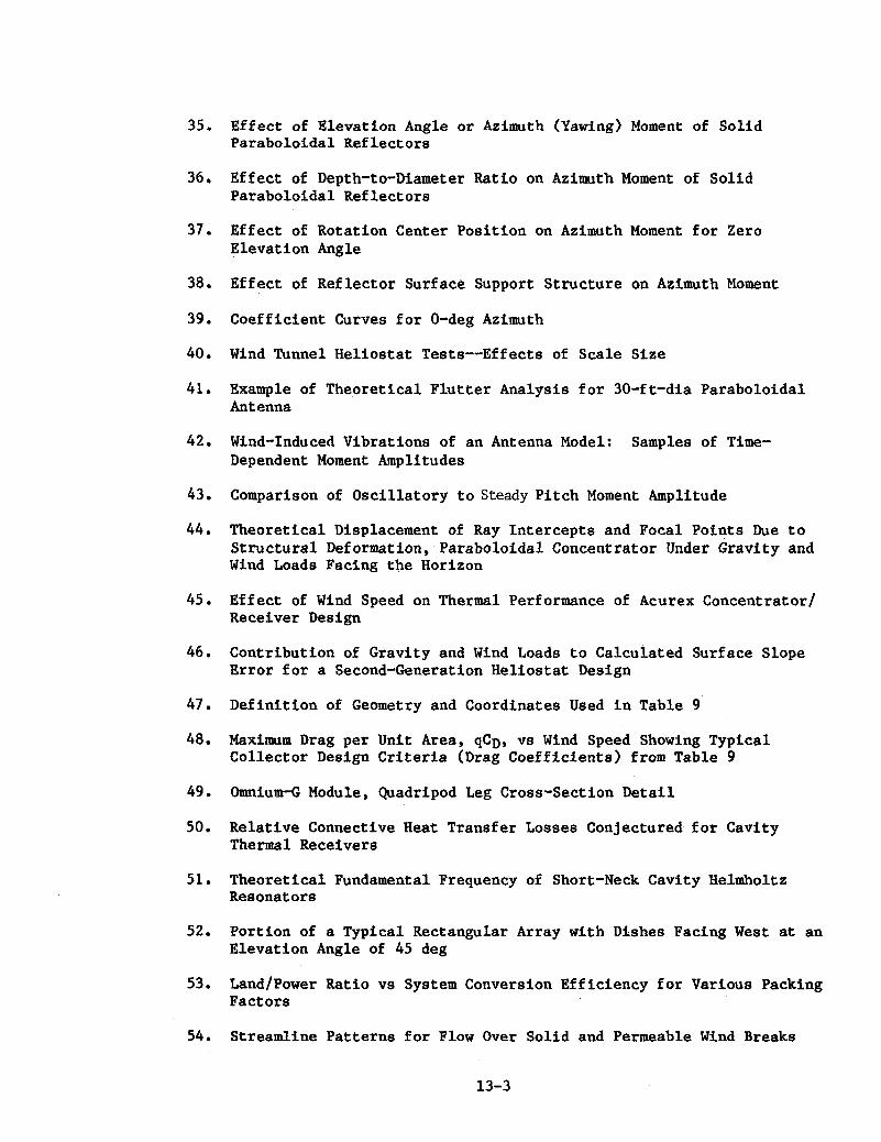


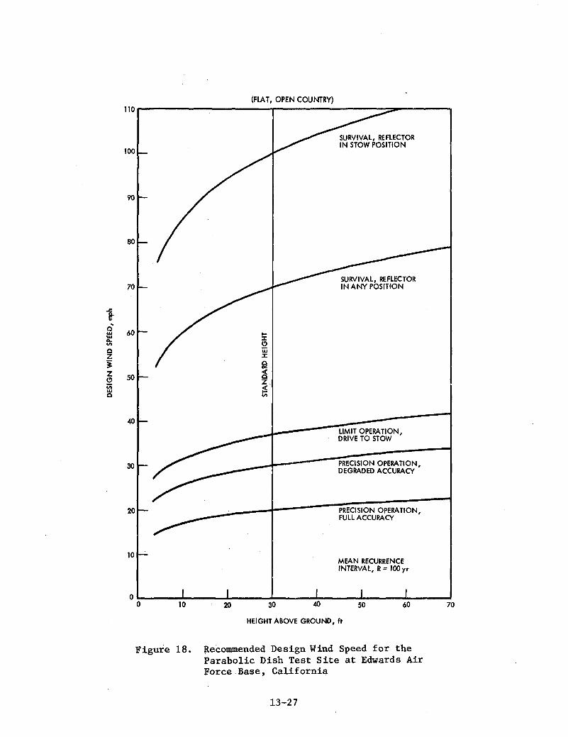


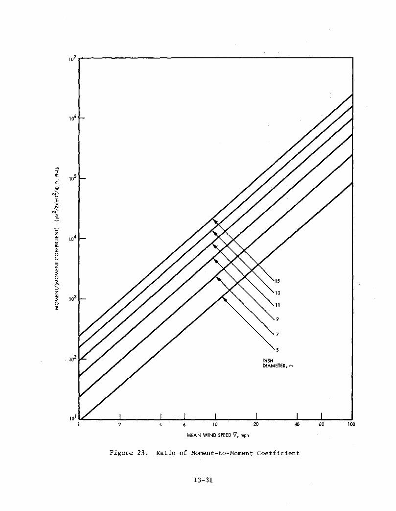


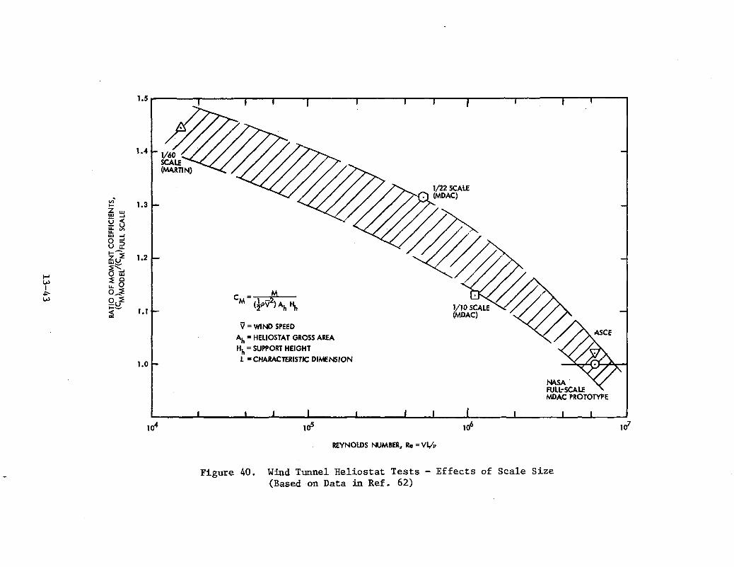


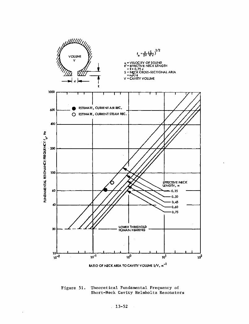


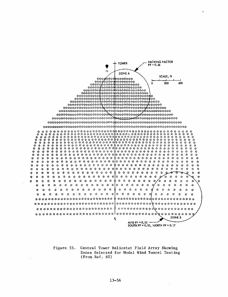


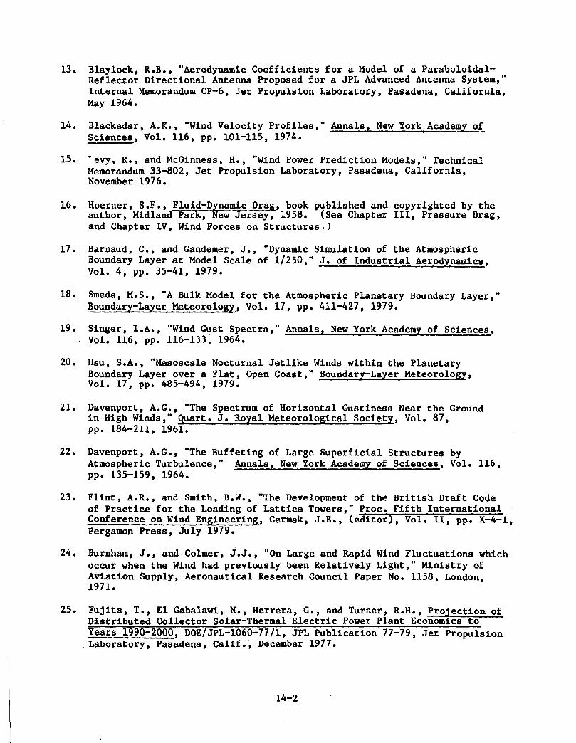


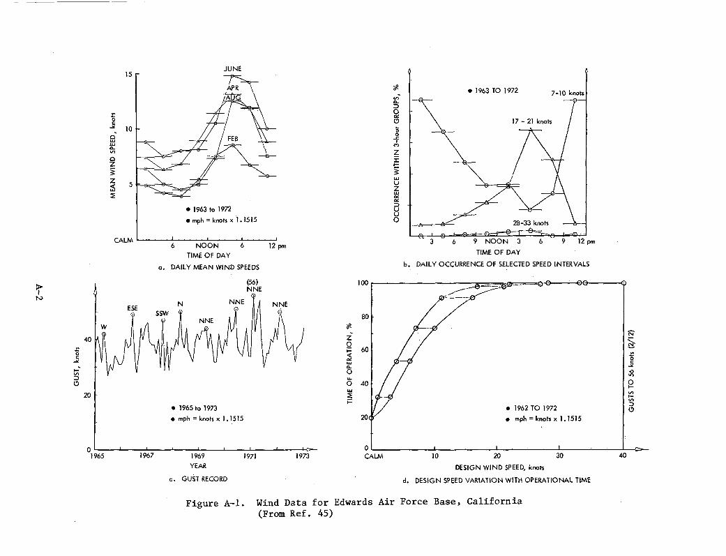


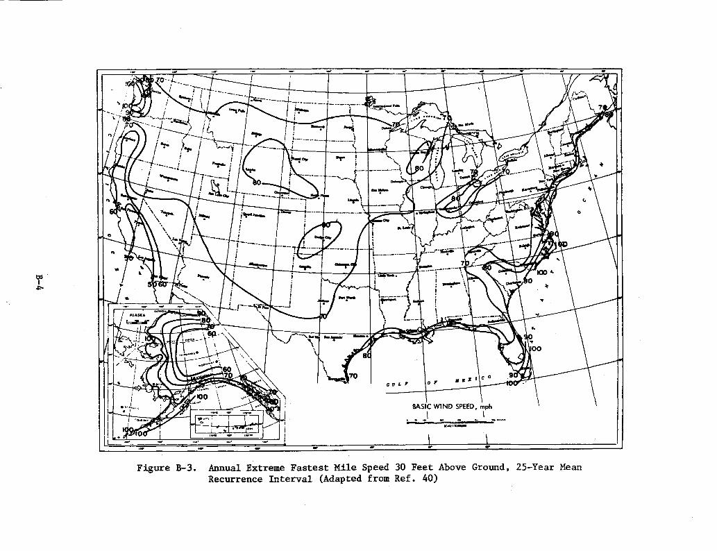


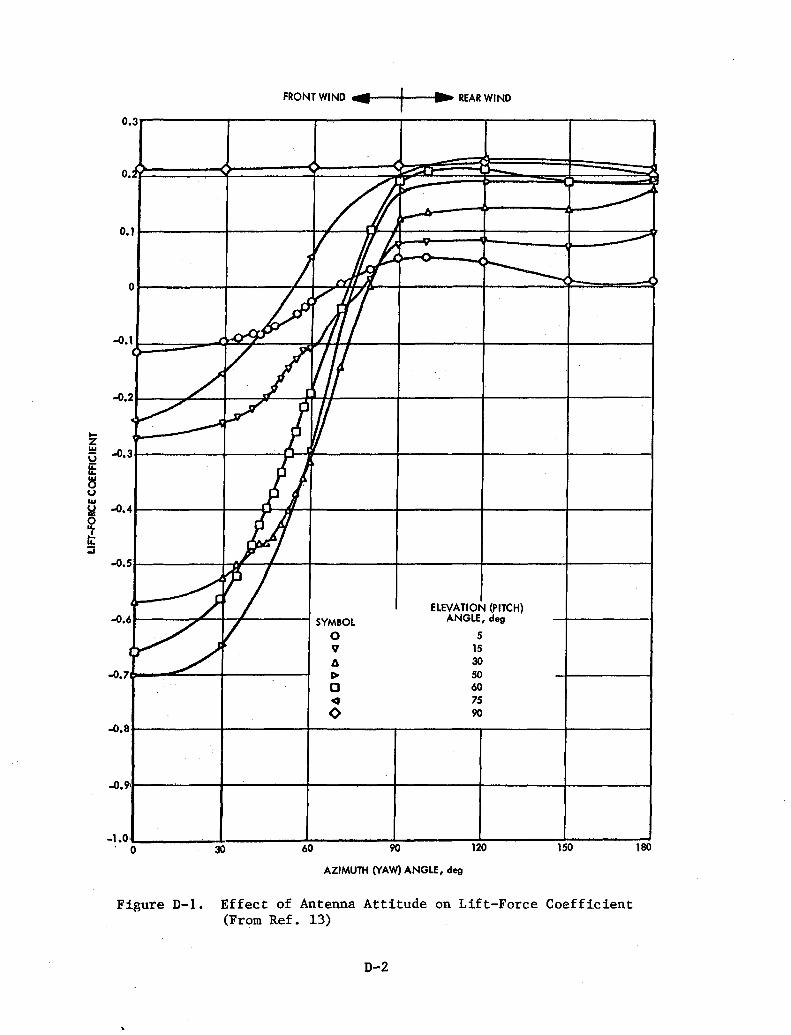


![Library Training [PDF Library]](https://static.documents.pub/doc/80x56/577d27501a28ab4e1ea39852/library-training-pdf-library.jpg)


