Wind Turbine Power Coefficient Identification Using the ...

Control Science and Engineering 2021; 5(1): 1-12

http://www.sciencepublishinggroup.com/j/cse

doi: 10.11648/j.cse.20210501.11

Wind Turbine Power Coefficient Identification Using the FAST Simulator Data and Design of Switching Multiple Model Predictive Control

Saman Saki1, *

, Ali Azizi2

1Department of Electrical Engineering, Iran University of Science and Technology, Tehran, Iran 2Department of Electrical Engineering, University of Kurdistan, Sanandaj, Iran

Email address:

*Corresponding author

To cite this article: Saman Saki, Ali Azizi. Wind Turbine Power Coefficient Identification Using the FAST Simulator Data and Design of Switching Multiple

Model Predictive Control. Control Science and Engineering. Vol. 5, No. 1, 2021, pp. 1-12. doi: 10.11648/j.cse.20210501.11

Received: June 14, 2020; Accepted: June 1, 2021; Published: June 21, 2021

Abstract: Due to the economic aspects and the global warming aims, the wind turbines have attracted a notable percent of the

research subjects in the recent decades. The motivation of this paper is identification of the Wind Turbine (WT) power coefficient

curve and improvement of the power tracking performance. To accomplish the first, using the steady state mode of the Fatigue

Aerodynamics Structures and Turbulence (FAST) simulator, we collect the necessary data pack and, then, identify the power

coefficient curve. For the second aim, a Multiple Model Predictive Control (MMPC) with a new adaptive structure is designed.

The model selection, through the constructed model bank, is handled based on the estimated wind speed using the

Newton-Rapshon (NR) and the kalman filter algorithm. The new adaptation law based on the Lyapunove theory damps the

hazardous chattering in the control signal coming from the sudden switching between controllers and models. This will improve

the wind turbine longevity. Afterwards, to investigate the effectiveness of the given method, the suggested algorithm is

implemented on the NREL 1.5 MW baseline WT using the FAST simulator. Finally, the simulation results validate the efficiency

of the suggested control system in the tracking error improvement, oscillation reduction in the generator torque and consequently

mechanical power, simultaneously.

Keywords: Multiple Model Predictive Control, Renewable Energy Systems, Oscillation Reduction,

Power Coefficient Identification

1. Introduction

Electrical power generation from wind energy has enhanced

rapidly from 20 years ago having a huge quota in different

energy categories. By 2013, the amount of 117.3 GW power

from the wind (including 110.7 GW onshore in addition to 6.6

GW offshore) was extracted in Europe. Based on Padmanaban

et al. [1], the capacity of the produced electrical power from

wind energy is such that it covers approximately 8% of the

Europe consumption rate. To raise this quota in the recent years,

20 kW to 2 MW wind turbines (WTs) have been technically

developed.

It has been proven that the researches in the way of designing

large WTs encounters with new different innovative concepts

and experimental tests (Crawford et al. [2]). Consequently,

different research fields have been appeared. In the research

fields, control engineering has a vital responsibility to extract

the most possible power known as maximum power point

tracking (MPPT), obtain safe mechanical and electrical system

known as reliability and increase the WT longevity and etc.

A variable-speed and variable-pitch wind energy

conversion system (WECS) works in three modes of the

energy production illustrated in the Figure 1 (Jain et al. [3]).

Based on the figure, for the wind speeds more than the cut-in

wind (shown with civ ), the WT starts energy production, for

the speeds less than the rated speed (shown with rv ), the rated

power is achieved. This wind speed interval named as the

partial load regime. The maximum power point tracking

(MPPT) is the target of the control system. Also, for the wind

speeds in the interval of rv to cov (called as the cut-out

wind speed) the full load regime is happened that the control

2 Saman Saki and Ali Azizi: Wind Turbine Power Coefficient Identification Using the FAST Simulator Data and

Design of Switching Multiple Model Predictive Control

system efforts to limit the output power. The WT is switched

off in the rest of the speeds.

Figure 1. The WT operation modes in different wind speeds.

The WT stochastic behavior of the WT causes an oscillation

in the both tracking and power curve which its reduction is the

control system concern. Consequently, the WT reliability and

efficiency and longevity strongly hang on the operation of the

control system in the wide range of the operating points.

Different control techniques (linear and nonlinear) are

presented in the literature. For example, to overcome the

limitations caused from the model nonlinearity, different

methods such as control based on kalman filter estimator

Tanvir et al. [11], Takagi-Sugeno (T-S) fuzzy modeling

Civelek et al. [12, 13] Hemeyine et al. [13], feedback

linearization Nguyen et al. [14], Multiple Model Predictive

Control (MMPC) in Li et al. [15], Soliman et al. [42] and Jain

et al. [3] is given. In the operating points of the partial load

regime, control methods like adaptive control Jabbari et al. [4]

and Asl et al. [5], sliding mode control (SMC) Beltran et al. [6],

linear quadratic gaussian (LQG) Munteanu et al. [19] and

model predictive control (MPC) Zhao et al. [7] have been

suggested. Furthermore, in the full load regime operating

points, MPC Zong et al. [8], robust control Mérida et al. [9]

and adaptive control Jafarnejadsani et al. [10] is suggested for

system safety, respectively. To diminish the output oscillation,

latest studies have revealed which the fluctuations coming

from the wind speed create transient loads in drive train part

and also oscillations appearing in either mechanical or

electrical power. Many presented solutions are given to

mitigate the fluctuation effects on WTs. An open loop

controller for WT pitch channel is suggested to deduce the

oscillations for the high speed winds conditions in Sun et al.

[22] and Hu et al. [23]. Also, individual pitch controller (IPC)

is the solution given in Bossanyi et al. [24], Bossanyi et al. [25]

and Zhang et al. [26]. In the reference Zhang et al. [27], a new

IPC is considered with respect to the generator active power

and WT azimuth angle and then, the presented simulations

demonstrate the efficiency of the suggested control system

using the spectral analysis.

This paper suggests a new soft switching multiple model

predictive control (MMPC) based on the gap metric

introduced in Georgiou et al. [16] and Vinnicombe et al. [17]

with a new structure to reduce the wind turbine power and

torque oscillation. The presence of a model and controller

bank makes it necessary: 1) to have a supervisor to certain

switching law among controller and 2) to guarantee the

stability of the closed loop control system. To handle these, we

use the estimated wind speed as a supervisor for switching

among controller. In this area, there have been presented many

methods such as Polynomial Thiringer et al. [28], neural

networks in (NN) Qiao et al. [29] and Li et al. [30], sensor

based support vector machine from Yang et al. [31] and Chen

et al. [21], adaptive neuro fuzzy interface systems (ANFS)

Mohandes et al. [32] and nonlinear estimator with

Newton-Raphson (NR) Johnson et al. [33] for the wind speed

estimation in the literature. In the all of these methods, having

power coefficient is a key problem and all assume it to be

certain. But in more cases, such as NREL 1.5 MW WT which

is understudy of this paper, the power coefficient model has

not been presented in the literature. In this field, different

methods for WT power coefficient identification like linear

curve model Diaf et al. [34], quadratic model Diaf et al. [35],

cubic law Lu et al. [36], linearized segmented model Lydia et

al. [37] and exponential equation Carrillo et al. [38] have been

used as parametric model to describe power coefficient. In

parameter estimation fields, literature Kusiak et al. [39] and

Kusiak et al. [40] present Least Squares (LS) method and

maximum likelihood (ML) methods, respectively. With

attention to the literature, we use nonlinear least square (NLS)

method to estimate the power coefficient of NREL 1.5 MW

baseline WT, in this paper. Moreover, using Lyapunov

stability analysis, an adaptation law is introduced that

adhering this law guarantees the stability of the closed loop

system.

Finally, to investigate the efficiency of the suggested

controller, The Fatigue Aerodynamic Structure and

Turbulence (FAST) simulator is chosen as a strong and

accurate WT nonlinear dynamic model made by National

Renewable Energy Laboratory (NREL) from the USA

Muteanu et al. [20].

This paper is prepared as follows: In the section 2, we

briefly introduce the dynamic model of the WT. In the next

section, the mathematical background of the robust control

tools named the gap metric is introduced. Section 4 provides

the suggested control system in details which includes the

main idea of the paper. In the section 5, the validation of the

proposed controller is given using the results getting from

FAST simulator. At the end of the paper, the section 6 gives

the conclusions.

2. Mathematical Background

In this part of the paper, we present the WT dynamic model

and then present the mathematical tool to measure the system

nonlinearity named as the gap metric.

A. The WT Dynamic Model

The comprehensive nonlinear dynamic model of a WT can

0 vci

vr v

co

Wind Speed (m/s)

Captu

red p

ow

er

(w)

Partial load regimeFull load

regime

Power Limitation

Control Science and Engineering 2021; 5(1): 1-12 3

be given with differential equation ( ),X f X u=ɺ in which

the state vector isT

r g gX x x Tω ω δ θ θ = ɺɺ ,

and the input control signal is _g desired refu T θ = . In the

state vector, the variables are as rotor angular velocity ( rω ),

generator angular velocity ( gω ), twist angle ( δ ), aft and fore

motion displacement ( x ) and its derivation ( xɺ ), pitch

actuator angle ( θ ) and its derivation ( θɺ ) and finally, the

generator torque ( gT ).

Also, the function ( )*f determine the nonlinearity part of

the differential equation. Furthermore, in the input signal

vector, the variables _g desiredT and refθ are the electrical

torque applied by the generator and the reference blade angle.

Finally, the equation ( )*f is as follows:

( )

( )

( )

2

2 2

_

, ,

,

1, ,

2

1 1

rr r w g sr s s

r r r r g r

g s gr s s

g g g g gg g

gr

g

rt tt r w

t t t

n n n ref

g g refT T

P v DD K

J J J N J

D TD K

J N J N JJ N

f X u N

K Dx x F v

M M M

T T

ω θ ωω δω

ωω δ

ωω

ω θ

ω θ ζω θ ω θ

τ τ

− + − − + − −= − − +− − +− +

ɺ

ɺ

(1)

Also, the parameters rJ , gJ , sD , sK and gN are the

rotor inertia, generator inertia, low speed side (LSS) damping

coefficient, LSS spring coefficient and gear ratio, respectively.

Furthermore, the parameter, tK , tD , tM are the tower

spring coefficient, tower damping coefficient and tower mass

respectively. Also, the pitch actuator natural frequency is

shown by nω . Moreover in the lowest equation, the

parameter Tτ is the generator time constant.

Clearly, it is a high nonlinear dynamic model that should be

linearized in order to design a linear controller in a special

operating point. To linearize equation (10) around a special

operating point, state variables should be calculated with

respect to the wind speed in the operating point with

assumption of 0X =ɺ . To handle this, in this paper, we use the

FAST simulator steady state analysis option to present linear

state space model in different operating points. Then, designed

controller is applied to detailed nonlinear dynamic model of

the FAST simulator.

B. The Gap Metric Theory

The comparison of the LTI systems is matter covering by

robust control theory. In this research field, the related

comparison is accomplished using the gap metric that it firstly

was presented in Georgiou et al. [16]. This concept was used

to investigate the feedback systems stability with uncertainty.

The definition of this criterion is:

( )1 21 2, K KK Kδ

∞= Π − Π

� (2)

Where 1K and 2K depict two linear systems and also

1KΠ is the orthogonal projections onto the graph space of

1K (more detail in Georgiou et al. [16]). With attention to the

fact that ( )1 2,K Kδ�

may be different from ( )2 1,K Kδ�

, we

consider:

( ) ( ) ( )( )1 2 1 2 2 1, max , , ,g gg P P P P P Pδ δ δ=��

(3)

with

( ) 1 21 2

1 2

, infgQ H

N NP P Q

M Mδ

∞∈∞

= −

�� (4)

Where, the transfer functions iN and iM are stable and:

1i i iP N M −= with i i i iN N M M I+ =ɶ ɶ (5)

Also note that ( ) ( )T

i iN s N s= −ɶ and ( ) ( )T

i iM s M s= −ɶ .

The similarity of Two linear systems is usually correct if the

gap value in Eq. 4 is approximately 0. Furthermore, the

notable difference in the response of two LTI systems leads to

the value of 1 for Eq. 4. Therefore, this tool is useful to be used

in multi model control systems to determine the suitable

number of the linear models when we want to model nonlinear

dynamic systems using linear models.

3. Proposed Control Strategy

A. Multiple Model Predictive Control

In this section, we design the switching MPC to make it

possible when transient from a local model to another one. In

details, assume the sub-model of mS as,

( ) ( ) ( )( )

1:

m m m m mm

m m m

x k A x k B u kS

y C x k

+ = + =

(6)

With state matrixes p p

mA R ×∈ andp q

mB R ×∈ . In the

mentioned equation, we demonstrate the state and input

vectors with

( ) pmx k R∈ and ( ) q

mu k R∈ respectively.

Also, with considering { }1,...,m M∈ as the number of the

sub-models, we write the MPC cost function for m -th

sub-model as Tao et al. [18]:



( )( ) ( )

( ) ( )( ) ( )

( ) ( ) ( )( ) { }

1

0

| |

| |

| |

.

1 | | |

| 1,..., 1

p

T Tm m mN

T Tm m m m

iT Tm m m

m m m m m

mm m

x k i k Q x k i k

J k u k i k R u k i k

x k N k P x k N k

s t

x k i k A x k i k B u k i k

u k i k U R i N

−

=

+ + = + + +

+ + +

+ + = + + +

+ ∈ ⊆ ∀ ∈ −

∑

(7)

In this equation, the positive semi-definite matrixes mQ

and mP with positive definite matrix of mR are chosen based

on the following theorem. Moreover, the parameter pN

determines the prediction horizon of the MPC.

In this paper, we firstly study the closed loop control system

stability in the local area and then expand that to the all of the

operating area with switching among sub-models.

Theorem. 1: if we consider the linear system given in Eq. (6)

with the assumptions of:

1) 0 χ∈

2) ( ) ( )m m m mA x k B u k χ+ ∈

3) ( ) ( )( )

( )( ) ( ) ( ), 0m m

Tm m m m

x k x k

where x k x k P x k

χ∀ ∈ Ψ

Ψ =

≻

4) ( ) ( ) ( )( )

( )( ) ( ) ( ) ( ) ( ),m m m m m

T Tm m m m m m m

x k A x k B u k

x k x k Q x k u k R u k

χ∀ ∈ Ψ + ≤

Ψ − −

Then, the MPC with the cost function of Eq. (7) is

asymptotically stable.

Proof. We consider the Lyapunov function to be the cost

function i.e. ( ) ( )mV k J k= . Therefore,

( )( ) ( )

( ) ( )( )( )

( ) ( ) ( )( ) ( )( ) ( )( ) ( )

( )( ) ( )( )

1

0

1 | 1 |

1 1 | 1 |

1 |

| |

| |

| |

| |

1 | |

Tm m m

NTm m m

i

m

Tm m m

Tm m m

Tm m m

Tm m m

m m

x k i k Q x k i k

V k u k i k R u k i k

x k N k

V k x k k Q x k k

u k k R u k k

x k N k Q x k N k

u k N k R u k N k

x k N k x k N k

−

=

+ + + + + = + + + + +

+Ψ + +

= −

−

+ + +

+ + +

+ Ψ + + − Ψ +

∑

(8)

Using ( ) ( ) ( )1 | | |m m m m mx k N k A x k N k B u k N k+ + = + + + ,

we can write:

( ) ( ) ( ) ( )( ) ( )( ) ( )( ) ( )

( ) ( )( )( )( )

1 | |

| |

| |

| |

| |

|

Tm m m

Tm m m

Tm m m

Tm m m

m m m m

m

V k V k x k k Q x k k

u k k R u k k

x k N k Q x k N k

u k N k R u k N k

A x k N k B u k N k

x k N k

+ = −

−

+ + +

+ + +

+ Ψ + + +

− Ψ +

(9)

With consideration of the assumption 4, the last four terms

of Eq. (9) become negative, which leads to the fact that

( ) ( )1V k V k +≻ .

The assumption of 4 is not always correct and, to make it

possible, we assume Tm m m m mA P A P Q− ≤ − (Rawlings et al.

[41]) for each of the local area.

To construct the closed loop control system, note that the

overall control system includes different stable MPC designed

based on the condition of theorem. 1. The switching manner

among the controllers in the controller bank is the next

challenge. To explain more, switching among MPCs can be

considered as switching among the related cost functions. As a

common challenge in switching control systems, it may cause

chattering or sometimes instability. In the next theorem, we

give a solution for stability under switching and chattering

reduction, simultaneously.

Theorem. 2: Consider a closed loop control system with

nonlinear dynamic system approximated using linear models

(6) extracted with consideration of the gap metric theory and

also local stable controllers designed by Theorem. 1.

Furthermore, assume:

1) ( )1k

m mP P f i P+ = + ∆

2) ( )1k

m mQ Q f i Q+ = + ∆

3) ( )1k

m mR R f i R+ = + ∆

4) ( )1,m m mgap S S ε+ ≤

where mε is a selective small and the function ( )kf i is

defined as,

( ) 1

1

sk kk sk k N

f ielse

η − − − <=

with [ ]0 1η ∈ . Then, the asymptotical stability of the

closed loop control is achieved under consideration of Eq. (10)

for MPC weight matrixes.

( )( ) ( ) ( ) ( ) ( ) ( )

( ) ( )

1

' 1 ' '

1

' ' ' ' ' '

' '

s s sm m m

sm

k k kT T Tm m m m m m

k k k k k k

kTm m

k k

x k P x k x k P x k x k Q x k

r k

u k u k

+

= + = =

= +

∆ − ∆ + ∆

∆ = −∑ ∑ ∑

∑ (10)

Proof. Because of the stability of the controllers mC and 1mC + when controlling sub-models mS and 1mS + ,

respectively, we can write using the assumptions:


( ) ( ) ( ) ( )( ) ( )( ) ( )

( ) ( ) ( ) ( )( ) ( )( ) ( )

1 1 1 1 1 1 1

1 1 1

1 1 1

: 1 1

: 1 1

T Tm m m m m m m

Tm m m

Tm m m

T Tm m m m m m m

Tm m m

Tm m m

S x k P x k x k P x k

x k Q x k

u k R u k

S x k P x k x k P x k

x k Q x k

u k R u k

+ + + + + + +

+ + +

+ + +

+ + ≤ − −

+ + ≤

−

−

(11)

The consideration of the inequality ( )1,m m mgap S S ε+ ≤ let

us to take ( ) ( )1m mx t x t+ ≈ and ( ) ( )1m mu t u t+ ≈ . Therefore,

the subtraction of the Eq. (11) gives:

( ) ( ) ( ) ( ) ( ) ( )( ) ( ) ( )( ) ( ) ( )

1 1T k T km m m m

T km m

T km m

x k f i P x k x k f i P x k

x k f i Q x k

u k f i R u k

+ ∆ + ≤ ∆

− ∆

− ∆

(1

2)

Based on the assumptions, with ( ) 0kf i > , we can write:

( ) ( ) ( ) ( )( ) ( )( ) ( )

1 1T Tm m m m

Tm m

Tm m

x k P x k x k P x k

x k Q x k

u k R u k

+ ∆ + ≤ ∆

− ∆

− ∆

(13)

Eq. (13) must be feasible in the even sampling time. Hence,

taking1m ms sk k k

+< < , we can write the following inequalities

(which are given for each sampling time in the system run

time):

( ) ( ) ( ) ( )( ) ( )( ) ( )

( ) ( ) ( ) ( )( ) ( )( ) ( )

1 1

1 1

m m m m

m m

m m

T Tm s m s m s m s

Tm s m s

Tm s m s

T Tm m m m

Tm m

Tm m

x k P x k x k P x k

x k Q x k

u k Ru k

x k P x k x k P x k

x k Q x k

u k Ru k

+ ∆ + ≤ ∆ − ∆ − ∆ + ∆ + ≤ ∆ − ∆ − ∆

⋮ (14)

A feasible selection may be to consider equality for each

inequality of Eq. (14). As a result, with the summation of the

whole of the equations in Eq. (14) and simultaneously the

assumption of n nR rI ×∆ = , Eq. (10) is achieved.

B. Determination of the Switching Law

The linear model characteristics of the WT are extremely

dependent to the wind speed. Thus, in this paper, we select the

switching rule based on the wind speed. On the other hand,

direct measurement of the wind speed is not possible Zhang et

al. [27]. Therefore, the wind speed estimation is a vital step in

the wind turbine control system. The overall wind estimator

block diagram is shown in the Figure 2. Based on this figure,

the measurements are the angular velocity and

electromagnetic torque of the generator. Next, a kalman filter

is used to estimate the LSS angular velocity and the

aerodynamic torque. Then, Newton-Raphson (NR) algorithm

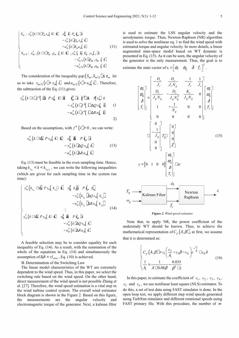
is used to solve the nonlinear eq. 1 to find the wind speed with

estimated torque and angular velocity. In more details, a linear

augmented state-space model based on WT dynamic is

presented in Eq. (15). As it can be seen, the angular velocity of

the generator is the only measurement. Thus, the goal is to

estimate the state vector of ˆ ˆˆ ˆxT

r g rTω ω δ =

.

[ ]

2

1 1

0

11 0 0

0 0 0 0

00

10

00

0

0 1 0 0

s s

r r g r r

r rs s s

g gg g g gg g

r rg

g g

r

g

r

D D

J J N J J

D D K

J N J NJ N

T TN

J T

y

T

ω ωω ωδ δ

ξ

ωω

υδ

− − − = −

− + +

= +

ɺ

ɺ

ɺ

ɺ

(15)

Figure 2. Wind speed estimator.

Note that, to apply NR, the power coefficient of the

understudy WT should be known. Thus, to achieve the

mathematical representation of ( ),pC λ β , at first, we assume

that it is determined as:

( )5

21 3 4 6

3

,

1 1 0.035

0.08 1

i

c

pi

i

cC c c c e c

λλ β β λλ

λ λ β β

− = − − + = − + +

(16)

In this paper, to estimate the coefficient of 1c , 2c , 3c , 4c ,

5c and 6c , we use nonlinear least square (NLS) estimator. To

do this, a set of test data using FAST simulator is done. In the

open loop test, we apply different step wind speeds generated

using TurbSim simulator and different rotational speeds using

FAST primary file. With this procedure, the number of m



data set containing ( ),pC λ β , λ and β is achieved. The

unknown parameters of Eq. (16) can be determined with

solving the optimization problem of:

( ) ( ) ( )( )( ) ( )( ) ( ) ( )( )

2

1

p p p p

1 ˆc , ,2

1 ˆ ˆC λ,β;c C λ,β C λ,β;c C λ,β2

m

p p

i

T

J C Cλ β λ β=

= −

= − −

∑ (17)

Here, c is the vector of unknown coefficients. The

nonlinear optimization problem of Eq. (17) should be solved

with numerical solutions. In this paper, Levenberg–Marquardt

algorithm is chosen to determine the optimum point. This

algorithm is composed from gradient descent (GD) and

Gauss–Newton algorithm. In the GD, the optimum point is

update using the gradient of Eq. (17) as:

( ) ( ) ( )( ) ( )p

p p

C λ,β;ccC λ,β;c C λ,β

c c

TJ ∂∂= −

∂ ∂ (18)

On the other hand, in Gauss–Newton algorithm, we have:

( ) ( ) ( )p

p p

C λ,β;cˆ ˆC λ,β;c h C λ,β;c h

c

∂+ = +

∂ (19)

where h is the update rate. Therefore, Eq. (19) can be

written as:

( ) ( ) ( )( ) ( ) ( )( )

( ) ( ) ( ) ( ) ( ) ( )

p p p p

p p

p p p p

1 ˆ ˆc h C λ,β;c h C λ,β C λ,β;c h C λ,β2

ˆ ˆC λ,β;c C λ,β;c1 ˆ ˆC λ,β;c h C λ,β C λ,β;c h C λ,β2 c c

T

T

J + = + − + −

∂ ∂ = + − + − ∂ ∂

(20)

Now we can write:

( ) ( ) ( )( ) ( ) ( ) ( )p p p

p

垐 ?C λ,β;c C λ,β;c C λ,β;cc hC λ,β;c C λ,β h

h c c c

T

T

p

J ∂ ∂ ∂∂ + = − + ∂ ∂ ∂ ∂

(21)

Getting ( )c h

0h

J∂ +=

∂, we have:

( ) ( ) ( ) ( ) ( )( )p p p

p p

ˆ ˆ ˆC λ,β;c C λ,β;c C λ,β;cˆh C λ,β;c C λ,β

c c c

T T ∂ ∂ ∂ = − − ∂ ∂ ∂

(22)

When c is near the optimal point, upgrading is based on Eq. (22), else it should be done based on GD. Finally,

( ) ( ) ( ) ( ) ( )( )1

p p p

p p

ˆ ˆ ˆC λ,β;c C λ,β;c C λ,β;cˆc c I C λ,β;c C λ,β

c c c

T T

µ

−

+ − ∂ ∂ ∂ = − − − ∂ ∂ ∂

(23)

Thus, the estimated power coefficients for NREL 1.5 MW

are calculated (Table 1). Also, the estimated power curve and

real data from FAST simulator is shown in Figure 3.

Table 1. The NREL 1.5 MW Wind Turbine Power Coefficient.

Parameter Value

1c 0.2939

2c 106.0000

3c 0.1542

4c 4.4340

5c 13.3000

6c 0.0001

Figure 3. The NREL 1.5 MW baseline estimated power coefficient curve.

0

10

20

30 0

5

10

15

20

0

0.1

0.2

0.3

0.4

0.5

λ(-)β(deg)

Cp

(-)


Figure 4. The suggested SSMMPC strategy.

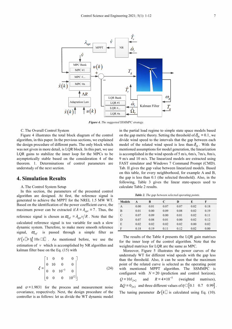
C. The Overall Control System

Figure 4 illustrates the total block diagram of the control

algorithm, in this paper. In the previous sections, we explained

the design procedure of different parts. The only block which

was not given in more detail, is LQR block. In this part, we use

LQR gains to stabilize the inner loop for the MPCs to be

asymptotically stable based on the consideration 4 of the

theorem. 1. Determinations of control parameters are

understudy of the next section.

4. Simulation Results

A. The Control System Setup

In this section, the parameters of the presented control

algorithm are designed. At first, the reference signal is

generated to achieve the MPPT for the NREL 1.5 MW WT.

Based on the identification of the power coefficient curve, the

maximum power can be extracted if 7optλ λ= = . Thus, the

reference signal is chosen as ref optv Rω λ= . Note that the

calculated reference signal is too variable for such a slow

dynamic system. Therefore, to make more smooth reference

signal, refω is passed through a simple filter as

( ) ( )1 10 1H s s= + . As mentioned before, we use the

estimation of v which is accomplished by NR algorithm and

kalman filter base on the Eq. (15) with

3

12

1 0 0 0

0 10 0 0

0 0 10 0

0 0 0 10

ξ −

=

(24)

and 1.9831υ = for the process and measurement noise

covariance, respectively. Next, the design procedure of the

controller is as follows: let us divide the WT dynamic model

in the partial load regime to simple state space models based

on the gap metric theory. Setting the threshold of 0.1thδ = , we

divide wind speed to the intervals that the gap between each

model of the related wind speed is less than thδ . With the

mentioned assumptions for model generation, the linearization

is accomplished in the wind speeds of 5 m/s, 6m/s, 7m/s, 8m/s,

9 m/s and 10 m/s. The linearized models are extracted using

FAST simulator and Windows 7 Command Prompt (CMD).

Tab. II gives the gap value between linearized models. Based

on this table, for every neighborhood, for example A and B,

the gap is less than 0.1 (the selected threshold). Also, in the

following, Table 3 gives the linear state-spaces used to

calculate Table 2 results.

Table 2. The gap between selected operating points.

Models A B C D E F

A 0.00 0.01 0.07 0.07 0.02 0.18

B 0.01 0.00 0.09 0.08 0.02 0.19

C 0.07 0.09 0.00 0.01 0.02 0.11

D 0.07 0.08 0.01 0.00 0.02 0.12

E 0.02 0.02 0.02 0.02 0.00 0.02

F 0.18 0.19 0.11 0.12 0.02 0.00

The results of the Table 4 presents the LQR gain matrixes

for the inner loop of the control algorithm. Note that the

weighted matrixes for LQR are the same as MPC.

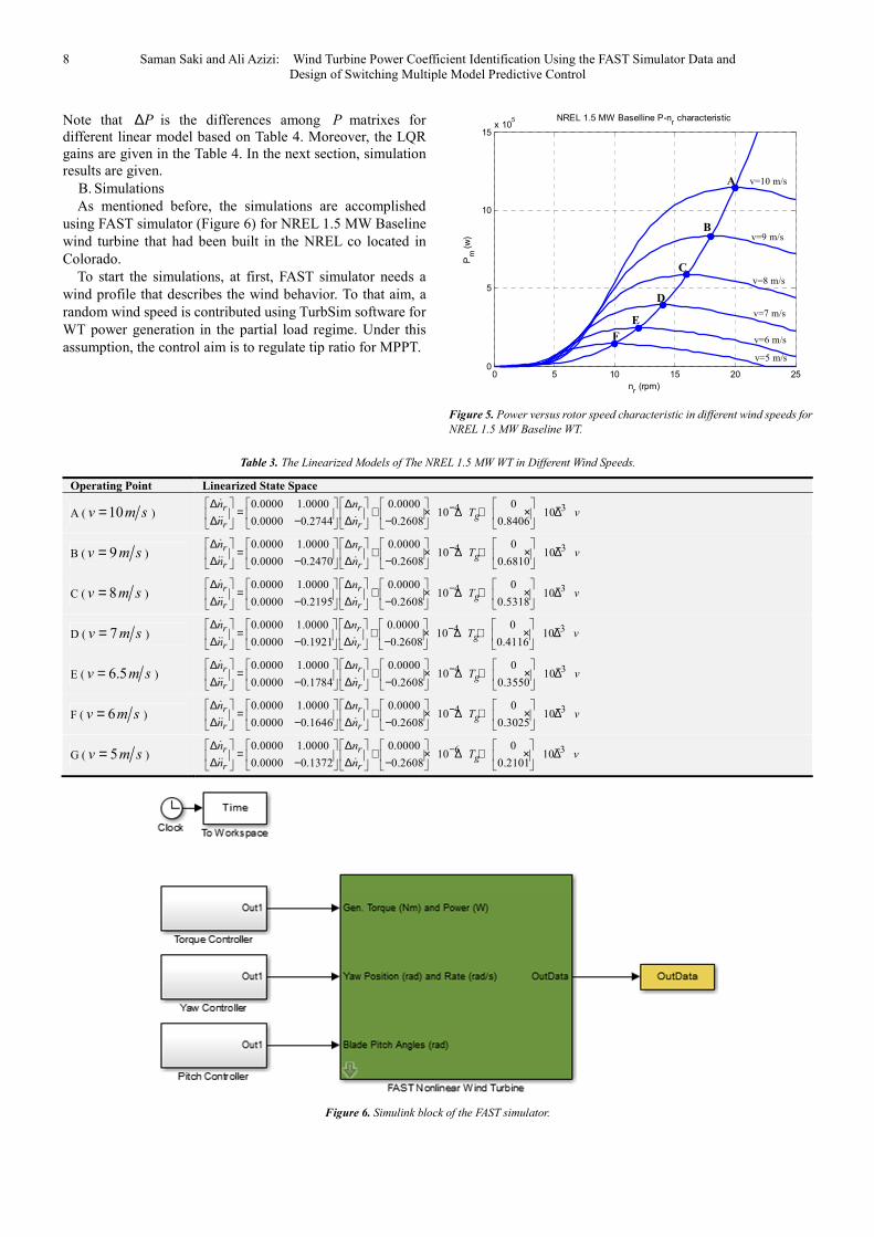
Moreover, Figure 5 illustrates the power curves of the

understudy WT for different wind speeds with the gap less

than the threshold. Also, it can be seen that the maximum

point of the related curve is selected as the operating point

with mentioned MPPT algorithm. The SSMMPC is

configured with 20N = (prediction and control horizon),

2 210Q I ×= and 5

4 10R−= × (weighted matrixes),

2 20Q ×∆ = and three different values of [ ]0.1 0.7 0.99η ∈ .

The tuning parameter ( )r k∆ is calculated using Eq. (10).



Note that P∆ is the differences among P matrixes for

different linear model based on Table 4. Moreover, the LQR

gains are given in the Table 4. In the next section, simulation

results are given.

B. Simulations

As mentioned before, the simulations are accomplished

using FAST simulator (Figure 6) for NREL 1.5 MW Baseline

wind turbine that had been built in the NREL co located in

Colorado.

To start the simulations, at first, FAST simulator needs a

wind profile that describes the wind behavior. To that aim, a

random wind speed is contributed using TurbSim software for

WT power generation in the partial load regime. Under this

assumption, the control aim is to regulate tip ratio for MPPT.

Figure 5. Power versus rotor speed characteristic in different wind speeds for

NREL 1.5 MW Baseline WT.

Table 3. The Linearized Models of The NREL 1.5 MW WT in Different Wind Speeds.

Operating Point Linearized State Space

A ( 10v m s= ) 4 30.0000 1.0000 0.0000 0

10 100.0000 0.2744 0.2608 0.8406

r rg

r r

n nT v

n n

− −∆ ∆ = + × ∆ + × ∆ ∆ ∆− −

ɺ

ɺɺ ɺ

B ( 9v m s= ) 4 30.0000 1.0000 0.0000 0

10 100.0000 0.2470 0.2608 0.6810

r rg

r r

n nT v

n n

− −∆ ∆ = + × ∆ + × ∆ ∆ ∆− −

ɺ

ɺɺ ɺ

C ( 8v m s= ) 4 30.0000 1.0000 0.0000 0

10 100.0000 0.2195 0.2608 0.5318

r rg

r r

n nT v

n n

− −∆ ∆ = + × ∆ + × ∆ ∆ ∆− −

ɺ

ɺɺ ɺ

D ( 7v m s= ) 4 30.0000 1.0000 0.0000 0

10 100.0000 0.1921 0.2608 0.4116

r rg

r r

n nT v

n n

− −∆ ∆ = + × ∆ + × ∆ ∆ ∆− −

ɺ

ɺɺ ɺ

E ( 6.5v m s= ) 4 30.0000 1.0000 0.0000 0

10 100.0000 0.1784 0.2608 0.3550

r rg

r r

n nT v

n n

− −∆ ∆ = + × ∆ + × ∆ ∆ ∆− −

ɺ

ɺɺ ɺ

F ( 6v m s= ) 4 30.0000 1.0000 0.0000 0

10 100.0000 0.1646 0.2608 0.3025

r rg

r r

n nT v

n n

− −∆ ∆ = + × ∆ + × ∆ ∆ ∆− −

ɺ

ɺɺ ɺ

G ( 5v m s= ) 6 30.0000 1.0000 0.0000 0

10 100.0000 0.1372 0.2608 0.2101

r rg

r r

n nT v

n n

− −∆ ∆ = + × ∆ + × ∆ ∆ ∆− −

ɺ

ɺɺ ɺ

Figure 6. Simulink block of the FAST simulator.

0 5 10 15 20 250

5

10

15x 10

5 NREL 1.5 MW Baselline P-nr characteristic

nr (rpm)

Pm

(w

)

v=5 m/s

v=6 m/s

v=7 m/s

v=8 m/s

v=9 m/s

v=10 m/sA

B

C

D

E

F


Figure 7. Comparison of the real and estimated aerodynamic torque.

To discuss about the output figures, let us start with

estimation part of the designed control system. Accordingly,

Figure 7 shows the estimation of the aerodynamic torque and

LSS rotational speed. Based on the Figures 7 and 8, it can be

understood that the kalman filter estimates the related states

suitable. Thus, in the following, Figure 9 presents satisfactory

wind speed estimation using NR algorithm via the kalman

filter outputs as its inputs.

The rest of the paper gives the tracking results of the

controller. As mentioned before, the estimated wind speed

handles the duty of supervisor for SSMMPC to select

operating sub-spaces. Using estimated wind speed as

supervisor, the simulations for tracking rotational speed in

LSS is shown in the Figure 10. The run time is set 600 seconds

to survey tracking results for enough wind speed variations.

The wind behavior is selected in which at the first half times, it

passes through almost all of the regions A, B, C, D, E, F and G.

In the next half time, it is approximately in the regions B, C, D

and E.

Figure 8. Comparison of the real and estimated angular velocity.

Figure 9. Comparison of the wind speed estimation using kalman filter and

NR algorithms.

Table 4. Local LQR feedback gains for the NREL 1.5 MW WT inner loop.

Operating Point LQR Gain LQR P Matrix

A ( 10v m s= ) 30.4894 1.6764 10− − ×

30.2495 0.766610

0.7666 2.6102

×

B ( 9v m s= ) 30.4883 1.8312 10− − ×

30.2317 0.766610

0.7666 2.8536

×

C ( 8v m s= ) 30.4871 2.0146 10− − ×

30.2143 0.766510

0.7665 3.1424

×

D ( 7v m s= ) 30.4856 2.2340 10− − ×

30.1978 0.766410

0.7664 3.4889

×

E ( 6.5v m s= ) 30.4847 2.3602 10− − ×

30.1899 0.766410

0.7664 3.6886

×

F ( 6v m s= ) 30.4838 2.4995 10− − ×

30.1822 0.766410

0.7664 3.9095

×

G ( 5v m s= ) 30.4817 2.8232 10− − ×

30.1679 0.766410

0.7664 4.4243

×

0 100 200 300 400 500 600-1

0

1

2

3

4

5

6

7

8x 10

5

Time(s)

Aero

dynam

ic T

orq

ue (

N.m

)

Real Torque

Estimated Torque

0 100 200 300 400 500 6000.8

1

1.2

1.4

1.6

1.8

2

2.2

Time(s)

ω r(rad/s

)

Real

Estimated

0 100 200 300 400 500 6002

4

6

8

10

12

14

Time(s)

v(m

/s)

Real

Estimated



Figure 10. Tracking results for LSS rotational speed (in rpm).

Figure 11. The SSMMPC control signal (generator torque).

Figure 12. The captured power from wind.

The simulations of Figure 10 depict the tracking for

different values ofη . As it can be seen, for 1η → , the LSS

speeds tracks the desired better than others. In the other words,

the LSS with 0.99η = is more near to the mean of the MPPT

based reference. In the following, let us investigate the applied

electromagnetic torque from generator and the captured power

of the wind. To do this, Figures 11 & 12 illustrate the

understudy signals. The simulation results of the control

signal shows that for 1η → , less fluctuations in the generator

torque is obtained which is the most important aim of this

paper. This matter is also concluded for the fluctuations of the

output power. Aside from time domain analysis, Figure 13

gives the power spectra of the generator torque. This figure

implies that for 1η → , the power spectra of the generator

torque lies down more which is equivalent to the fluctuation

reduction.

Figure 13. The power spectra of the control signal.

Figure 14. The sub-model selection scenario.

To figure out the procedure of the switching among sub

models and related controllers, Figure 14 gives the results of

the switching for the model updating and Figure 15 presents

the behavior of the adaptation law of the control system.

Deeping in both Figures 14 & 15, it can be seen that in the

interval of 0 to 300 seconds, that wind speed changes fast, the

variations of the control law is far more than its variations in

the time interval of 301 to 600 seconds. In fact, less transients

among sub-models consequence less change in the adaptation

law signal.

0 100 200 300 400 500 6000

5

10

15

20

25

Time(s)

nr

MPPT Ref

η=0.0

η=0.1

η=0.7

η=0.99

0 100 200 300 400 500 600-4000

-2000

0

2000

4000

6000

8000

10000

Time(s)

Tg(N

.m)

η=0.0

η=0.1

η=0.7

η=0.99

0 100 200 300 400 500 600-5

0

5

10

15x 10

5

Time(s)

Pg(W

)

η=0.0

η=0.1

η=0.7

η=0.99

0 50 100 150 200 250 300 350 400 450 500-50

0

50

100

Frequency (Hz)

Pow

er/

Fre

quency (

dB

/Hz)

η=0.0

η=0.1

η=0.7

η=0.99

0 100 200 300 400 500 600B

C

D

E

F

G

Time(s)

Sub-m

odel in

dex


Figure 15. The illustration of the adaptation law.

5. Conclusion

In this paper, a new direct adaptive SSMMPC technique to

control the NREL 1.5 MW wind turbine in the partial load

regime for high tracking performance and reliability was

proposed. Using a mathematical tool, called as the gap metric,

the partial load regime was divided into 7 operating points that

the gap between each neighborhood was less than a suitable

threshold. Next, a model bank and controller bank were

designed to control the closed loop system. Firstly, the

stability of each local model and controller was guaranteed

using theorem. 1. Next, due to the high sensitivity of the

control loop in switching systems, the classical switching

(hard switching) may causes chattering or even instability in

the cases of extreme variations of the wind speed. To solve this

problem, a new adaptation law was introduced based on

Lyapunov stability analysis to guarantee the global stability of

the total closed-loop system. Finally, the simulations prove the

effectiveness of the proposed control algorithm to achieve

high tracking performance and also more reliability of the

generator with torque oscillation reduction.

Appendix

The NREL 1.5 MW WT parameters are given in the Table 5.

Table 5. The NREL 1.5 MW WT Parameters Used in Simulations (Kalman

Filter).

Parameter Value

Number of Blades 3

Rotor diameter 70m

Hub height 84.3m

Rated power 1.5MW

Turbine total inertia 5 24.4532 10 .kg m×

Gearbox ratio 87.965

Air density 31.225kg m

Rotor inertia 253.036kg m

Hub Inertia 3 234.6 10 kg m×

References

[1] Padmanaban S, Blaabjerg F, Wheeler P, Ojo J. O and Ertas A. H (2017) High-voltage dc-dc converter topology for pv energy utilization—Investigation and implementation. Electric Power Components and Systems, 45 (3), pp. 221-232.

[2] Crawford R. H (2009) Life cycle energy and greenhouse emissions analysis of wind turbines and the effect of size on energy yield. Renewable and Sustainable Energy Reviews, 13 (9), pp. 2653-2660.

[3] Jain A, Schildbach G, Fagiano L and Morari M (2015) On the design and tuning of linear model predictive control for wind turbines. Renewable Energy, 80, pp. 664-673.

[4] Jabbari Asl H and Yoon J (2017) Adaptive control of variable-speed wind turbines for power capture optimisation. Transactions of the Institute of Measurement and Control, 39 (11), pp. 1663-1672.

[5] Asl H. J and Yoon J (2016) Power capture optimization of variable-speed wind turbines using an output feedback controller. Renewable Energy, 86, pp. 517-525.

[6] Beltran B, Ahmed-Ali T and Benbouzid M. E. H (2008) High-order sliding-mode control of variable-speed wind turbines. IEEE Transactions on Industrial electronics, 56 (9), pp. 3314-3321.

[7] Zhao H, Wu Q, Guo Q, Sun H and Xue Y (2015) Distributed model predictive control of a wind farm for optimal active power controlpart II: Implementation with clustering-based piece-wise affine wind turbine model. IEEE Transactions on Sustainable Energy, 6 (3), pp. 840-849.

[8] Zong Y, Kullmann D, Thavlov A, Gehrke O and Bindner H. W (2012) Application of model predictive control for active load management in a distributed power system with high wind penetration. IEEE Transactions on Smart Grid, 3 (2), pp. 1055-1062.

[9] Mérida J, Aguilar L. T, and Dávila, J (2014) Analysis and synthesis of sliding mode control for large scale variable speed wind turbine for power optimization. Renewable Energy, 71, pp. 715-728.

[10] Jafarnejadsani H, Pieper J and Ehlers J (2013) Adaptive control of a variable-speed variable-pitch wind turbine using radial-basis function neural network. IEEE transactions on control systems technology, 21 (6), pp. 2264-2272.

[11] Tanvir, Aman A., and Adel Merabet. "Artificial neural network and Kalman filter for estimation and control in standalone induction generator wind energy DC microgrid." Energies 13.7 (2020): 1743.

[12] Civelek, Zafer. "Optimization of fuzzy logic (Takagi-Sugeno) blade pitch angle controller in wind turbines by genetic algorithm." Engineering Science and Technology, an International Journal 23.1 (2020): 1-9.

[13] Hemeyine, Ahmed Vall, et al. "Robust Takagi Sugeno Fuzzy Models control for a Variable Speed Wind Turbine Based a DFI-Generator." International Journal of Intelligent Engineering and Systems 13.3 (2020): 90-100.

0 100 200 300 400 500 600-0.5

-0.4

-0.3

-0.2

-0.1

0

0.1

0.2

0.3

0.4

0.5

Time(s)

∆R



[14] Nguyen, Anh Tan, and Dong-Choon Lee. "LVRT Control based on Partial State-Feedback Linearization for SCIG Wind Turbine Systems." 2020 IEEE Energy Conversion Congress and Exposition (ECCE). IEEE, 2020.

[15] Li, Hongwei, et al. "Adaptive multi-model switching predictive active power control scheme for wind generator system." Energies 13.6 (2020): 1329.

[16] Georgiou T. T and Smith M. C (1989) December. Optimal robustness in the gap metric. In Proceedings of the 28th IEEE Conference on Decision and Control, (pp. 2331-2336). IEEE.

[17] Vinnicombe G (1993) Frequency domain uncertainty and the graph topology. IEEE Transactions on Automatic Control, 38 (9), pp. 1371-1383.

[18] Tao X, Li N and Li S (2016) Multiple model predictive control for large envelope flight of hypersonic vehicle systems. Information Sciences, 328, pp. 115-126.

[19] Munteanu I, Cutululis N. A, Bratcu A. I and Ceangă E (2005) Optimization of variable speed wind power systems based on a LQG approach. Control engineering practice, 13 (7), pp. 903-912.

[20] Muteanu I, Bratcu A. I, Cutululis N. A and Ceangă E (2008) Optimal control of wind energy systems.

[21] Chen K and Yu J (2014) Short-term wind speed prediction using an unscented Kalman filter based state-space support vector regression approach. Applied Energy, 113, pp. 690-705.

[22] Sun T, Chen Z and Blaabjerg F (2005) Flicker study on variable speed wind turbines with doubly fed induction generators. IEEE Transactions on Energy Conversion, 20 (4), pp. 896-905.

[23] Hu W, Chen Z, Wang Y and Wang Z (2009) Flicker mitigation by active power control of variable-speed wind turbines with full-scale back-to-back power converters. IEEE Transactions on Energy Conversion, 24 (3), pp. 640-649.

[24] Bossanyi E. A, (2003) Individual blade pitch control for load reduction. Wind Energy: An International Journal for Progress and Applications in Wind Power Conversion Technology, 6 (2), pp. 119-128.

[25] Bossanyi E. A (2005) Further load reductions with individual pitch control. Wind Energy: An International Journal for Progress and Applications in Wind Power Conversion Technology, 8 (4), pp. 481-485.

[26] Zhang Y, Chen Z, Cheng M and Zhang J (2011) September. Mitigation of fatigue loads using individual pitch control of wind turbines based on FAST. In 2011 46th International Universities' Power Engineering Conference (UPEC) (pp. 1-6). VDE.

[27] Zhang Y, Chen Z, Hu W and Cheng M (2014) Flicker mitigation by individual pitch control of variable speed wind turbines with DFIG. IEEE Transactions on Energy Conversion, 29 (1), pp. 20-28.

[28] Thiringer T and Petersson A (2005) Control of a variable-speed pitch regulated wind turbine.

[29] Qiao W (2009) June Echo-state-network-based real-time wind speed estimation for wind power generation. In 2009 International Joint Conference on Neural Networks (pp. 2572-2579). IEEE.

[30] Li H, Shi K. L and McLaren P. G (2005) Neural-network-based sensorless maximum wind energy capture with compensated power coefficient. IEEE transactions on industry applications, 41 (6), pp. 1548-1556.

[31] Yang X, Han X, Xu L and Liu Y (2006) December. Soft sensor based on support vector machine for effective wind speed in large variable wind. In 2006 9th International Conference on Control, Automation, Robotics and Vision (pp. 1-4). IEEE.

[32] Mohandes M, Rehman S and Rahman S. M (2011) Estimation of wind speed profile using adaptive neuro-fuzzy inference system (ANFIS). Applied Energy, 88 (11), pp. 4024-4032.

[33] Johnson K. E, Pao L. Y, Balas M. J and Fingersh L. J (2006) Control of variable-speed wind turbines: standard and adaptive techniques for maximizing energy capture. IEEE Control Systems Magazine, 26 (3), pp. 70-81.

[34] Diaf S, Belhamel M, Haddadi M and Louche A (2008) Technical and economic assessment of hybrid photovoltaic/wind system with battery storage in Corsica island. Energy policy, 36 (2), pp. 743-754.

[35] Diaf S, Notton G, Belhamel M, Haddadi M and Louche A (2008) Design and techno-economical optimization for hybrid PV/wind system under various meteorological conditions. Applied Energy, 85 (10), pp. 968-987.

[36] Lu L, Yang H and Burnett J (2002) Investigation on wind power potential on Hong Kong islands—an analysis of wind power and wind turbine characteristics. Renewable Energy, 27 (1), pp. 1-12.

[37] Lydia M, Selvakumar A. I, Kumar S. S and Kumar G. E. P (2013) Advanced algorithms for wind turbine power curve modeling. IEEE Transactions on sustainable energy, 4 (3), pp. 827-835.

[38] Carrillo C, Montaño A. O, Cidrás, J and Díaz-Dorado, E (2013) Review of power curve modelling for wind turbines. Renewable and Sustainable Energy Reviews, 21, pp. 572-581.

[39] Kusiak A, Zheng H and Song Z (2009) On-line monitoring of power curves. Renewable Energy, 34 (6), pp. 1487-1493.

[40] Kusiak A, Zheng H and Song Z (2009) Models for monitoring wind farm power. Renewable Energy, 34 (3), pp. 583-590.

[41] Rawlings J. B and Muske K. R (1993) The stability of constrained receding horizon control. IEEE transactions on automatic control, 38 (10), pp. 1512-1516.

[42] Soliman M, Malik O. P and Westwick D. T (2011) Multiple model predictive control for wind turbines with doubly fed induction generators. IEEE Transactions on Sustainable Energy, 2 (3), pp. 215-225.

Date post:	18-Dec-2021
Category:	Documents
Upload:	others
View:	2 times
Download:	0 times

Wind Turbine Power Coefficient Identification Using the ...

Documents