20 Wind Turbines with Permanent Magnet Synchronous Generator and Full-Power Converters: Modelling, Control and Simulation Rui Melício 1 , Victor M. F. Mendes 2 and João P. S. Catalão 3 1 CIEEE – Center for Innovation in Electrical and Energy Engineering 2 ISEL – Instituto Superior de Engenharia de Lisboa 3 UBI – University of Beira Interior Portugal 1. Introduction Research about dynamic models for grid-connected wind energy conversion systems is one of the challenges to achieve knowledge for the ongoing change due to the intensification of using wind energy in nowadays. This book chapter is an involvement on those models, but dealing with wind energy conversion systems consisting of wind turbines with permanent magnet synchronous generators (PMSG) and full-power converters. Particularly, the focus is on models integrating the dynamic of the system as much as potentially necessary in order to assert consequences on the operation of system. In modelling the energy captured from the wind by the blades, disturbance imposed by the asymmetry in the turbine, the vortex tower interaction, and the mechanical eigenswings in the blades are introduced in order to assert a more accurate behaviour of wind energy conversion systems. The conversion system dynamic comes up from modelling the dynamic behaviour due to the main subsystems of this system: the variable speed wind turbine, the mechanical drive train, and the PMSG and power electronic converters. The mechanical drive train dynamic is considered by three different model approaches, respectively, one- mass, two-mass or three-mass model approaches in order to discuss which of the approaches are more appropriated in detaining the behaviour of the system. The power electronic converters are modelled for three different topologies, respectively, two-level, multilevel or matrix converters. The consideration of these topologies is in order to expose its particular behaviour and advantages in what regards the total harmonic distortion of the current injected in the electric network. The electric network is modelled by a circuit consisting in a series of a resistance and inductance with a voltage source, respectively, considering two hypotheses: without harmonic distortion or with distortion due to the third harmonic, in order to show the influence of this third harmonic in the converter output electric current. Two types of control strategies are considered in the dynamic models of this book chapter, respectively, through the use of classical control or fractional-order control. Case studies were written down in order to emphasize the ability of the models to simulate new contributions for studies on grid-connected wind energy conversion systems. www.intechopen.com
Transcript
20
Wind Turbines with Permanent Magnet Synchronous Generator and Full-Power
Converters: Modelling, Control and Simulation
Rui Melício1, Victor M. F. Mendes2 and João P. S. Catalão3 1CIEEE – Center for Innovation in Electrical and Energy Engineering
2ISEL – Instituto Superior de Engenharia de Lisboa 3UBI – University of Beira Interior
Portugal
1. Introduction
Research about dynamic models for grid-connected wind energy conversion systems is one
of the challenges to achieve knowledge for the ongoing change due to the intensification of
using wind energy in nowadays. This book chapter is an involvement on those models, but
dealing with wind energy conversion systems consisting of wind turbines with permanent
magnet synchronous generators (PMSG) and full-power converters. Particularly, the focus is
on models integrating the dynamic of the system as much as potentially necessary in order
to assert consequences on the operation of system.
In modelling the energy captured from the wind by the blades, disturbance imposed by the
asymmetry in the turbine, the vortex tower interaction, and the mechanical eigenswings in
the blades are introduced in order to assert a more accurate behaviour of wind energy
conversion systems. The conversion system dynamic comes up from modelling the dynamic
behaviour due to the main subsystems of this system: the variable speed wind turbine, the
mechanical drive train, and the PMSG and power electronic converters. The mechanical
drive train dynamic is considered by three different model approaches, respectively, one-
mass, two-mass or three-mass model approaches in order to discuss which of the
approaches are more appropriated in detaining the behaviour of the system. The power
electronic converters are modelled for three different topologies, respectively, two-level,
multilevel or matrix converters. The consideration of these topologies is in order to expose
its particular behaviour and advantages in what regards the total harmonic distortion of the
current injected in the electric network. The electric network is modelled by a circuit
consisting in a series of a resistance and inductance with a voltage source, respectively,
considering two hypotheses: without harmonic distortion or with distortion due to the third
harmonic, in order to show the influence of this third harmonic in the converter output
electric current. Two types of control strategies are considered in the dynamic models of this
book chapter, respectively, through the use of classical control or fractional-order control.
Case studies were written down in order to emphasize the ability of the models to simulate
new contributions for studies on grid-connected wind energy conversion systems.
www.intechopen.com
Wind Turbines
466
Particularly, the contexts of possible malfunctions is an added contribution for the studies
on: the pitch angle control of the turbine blades, malfunction characterized by momentarily
imposing the position of wind gust on the blades; the power electronic converters control,
malfunction characterized by an error choice assumed on the voltage vectors for the power
electronic converter. Hence, simulation results of the dynamic models regarding the
behaviours not only due to the fact that wind energy is not a controllable source of energy,
but also due to possible malfunctions of devices that drive the control on wind energy
conversion systems, are presented and discussed. Also, the simulation for the use of
fractional-order control is a new contribution on the studies for controlling grid-connected
wind energy conversion systems. A comparison between the classical control and the
fractional-order control strategies in what regards the harmonic content, computed by the
Discrete Fourier Transform, injected into the electric network is presented. The simulations
of the mathematical models considered in this book chapter are implemented in
Matlab/Simulink.
2. Modelling
2.1 Wind speed
The energy stored in the wind is in a low quality form of energy. Many factors influence the
behaviour of the wind speed so it is modelised as a source intermittent and variable of
energy and somehow characterized as random variable in magnitude and direction (Chen &
Spooner, 2001). Although of the characterisation of wind energy as random variable, for the
purpose of this book chapter the wind speed can be modelled as a deterministic sum of
harmonics with frequency in range of 0.1–10 Hz (Xing et al., 2006), given by
0 1 sin( )n nn
u u A tω⎡ ⎤= +⎢ ⎥⎣ ⎦∑ (1)
where u is the wind speed, 0u is the average wind speed, nA is the magnitude of the
eigenswing n, nω is the eigenfrequency of the eigenswing n. The wind speed variation put
into effect an action on the physical structure of a wind turbine (Akhmatov et al., 2000). This
action causes a reaction of the physical structure, introducing mechanical effects perturbing
the energy conversion. Hence, further consideration due to the wind speed variation was
studied in order to better characterize the mechanical power associated with the energy
conversion over the rotor due to the action on the physical structure.
2.2 Wind turbine
The mechanical power in the nonappearance of mechanical effects, influencing the energy
conversion, on the physical structure of a wind turbine, is computed by
31
2tt t pP A u cρ= (2)
where ttP is the mechanical power associated with the energy capture from the wind by the
blades, ρ is the air density, tA is the area covered by the rotor blades, and pc is the power
coefficient.
www.intechopen.com
Wind Turbines with Permanent Magnet Synchronous Generator and Full-Power Converters: Modelling, Control and Simulation
467
The power coefficient pc is a function of the pitch angle θ of rotor blades and of the tip speed ratio λ , which is the ratio between blade tip speed and wind speed value upstream of the rotor, given by
t tR
u
ωλ = (3)
where tω is the rotor angular speed at the wind turbine, tR is the radius of the area covered by the blades. The computation of the power coefficient requires the use of blade element theory and the knowledge of blade geometry or the use of real wind turbine characteristic table. In this book chapter, the numerical approximation ascribed by (Slootweg et al., 2003) is followed. The power coefficient in this numerical approximation is given by
2.14
18.4151
0.73 0.58 0.002 13.2 ip
i
c eλθ θλ
−⎛ ⎞= − − −⎜ ⎟⎝ ⎠ (4)
3
1
1 0.003
( 0.02 ) ( 1)
iλλ θ θ
=−− +
(5)
The maximum power coefficient is at null pitch angle and for this numerical approximation it is equal to
max( (0), 0) 0.4412optpc λ = (6)
with the optimal tip speed ratio at null pitch angle equal to
(0) 7.057optλ = (7)
The maximum pitch angle for the numerical approximation is 55º, and the minimum power coefficient is equal to
min ( (55), 55) 0.0025pc λ = (8)
with a tip speed ratio equal to
(55) 3.475λ = (9)
The conversion of wind energy into mechanical energy over the rotor of a wind turbine is influenced by various forces acting on the blades and on the tower of the wind turbine (e.g. centrifugal, gravity and varying aerodynamic forces acting on blades, gyroscopic forces acting on the tower), introducing mechanical effects influencing the energy conversion. Those mechanical effects have been modelled by eigenswings mainly due to the following phenomena: asymmetry in the turbine, vortex tower interaction, and mechanical eigenswing in the blades. The mechanical power over the rotor of a wind turbine has been modelled as sum of harmonic terms multiplied by the power given by (2), where the mechanical eigenswings define the harmonics. In this book chapter, the model developed in (Xing et al., 2006)-(Akhmatov et al., 2000) is followed, where the further consideration due to the action on the physical structure confers a mechanical power over the rotor given by
www.intechopen.com
Wind Turbines
468
3 2
1 1
1 ( ) ( )t tt n nm nm nn m
P P A a g t h t= =
⎡ ⎤⎛ ⎞= +⎢ ⎥⎜ ⎟⎢ ⎥⎝ ⎠⎣ ⎦∑ ∑ (10)
( )0sin ( ') '
t
nm n nmg m t dtω ϕ= +∫ (11)
where tP is the mechanical power of the wind turbine disturbed by the mechanical
eigenswings, m is the order of the harmonic of an eigenswing, nmg is the distribution of the
m-order harmonic in the eigenswing n, nma is the normalized magnitude of nmg , nh is the
modulation of eigenswing n, nmϕ is the phase of the m-order harmonic in the eigenswing n.
The eigenfrequency range of the wind turbine model is considered to be from 0.1 to 10 Hz.
The values used for computing tP (Akhmatov et al., 2000) are given in Table 1.
n
Source nA nω hn m nma nmϕ
1 4/5 0 1 Asymmetry 0.01
ωt
1 2 1/5 π/2
1 ½ 0 2
Vortex towerinteraction
0.08
3 ωt
1 2 ½ π /2
3 Blades 0.15 9 π 1/2 (g11+g21) 1 1 0
Table 1. Mechanical eigenswings excited in the wind turbine
2.3 One mass drive train
In a one-mass drive train model all inertia components are lumped together, i.e., modelled as a single rotating mass. The equation for the one-mass model is based on the second law of Newton, deriving the state equation for the rotor angular speed at the wind turbine, given by
( )1tt g
dT T
dt J
ω = − (12)
where J is the moment of inertia for blades, hub and generator, tT is the mechanical
torque, gT is the electric torque.
2.4 Two mass drive train
The equations for the two-mass model are based on the torsional version of the second law
of Newton, deriving the state equation for the rotor angular speed at the wind turbine and
for the rotor angular speed at the generator, given by
( )1tt dt at ts
t
dT T T T
dt J
ω = − − − (13)
www.intechopen.com
Wind Turbines with Permanent Magnet Synchronous Generator and Full-Power Converters: Modelling, Control and Simulation
469
( )1gts dg ag g
g
dT T T T
dt J
ω = − − − (14)
where tJ is the moment of inertia for blades and hub, dtT is the resistant torque in the wind
turbine bearing, atT is the resistant torque in the hub and blades due to the viscosity of the
airflow, tsT is the torque of torsional stiffness, gω is the rotor angular speed at the
generator, gJ is the generator moment of inertia, dgT is the resistant torque in the generator
bearing, agT is the resistant torque due to the viscosity of the airflow in the generator. A
comparative study of wind turbine generator system using different drive train models
(Muyeen et al., 2006) has shown that the two-mass model may be more suitable for transient
stability analysis than one-mass model. The simulations in this book chapter are in
agreement with this comparative study in what regards the discarding of one-mass model.
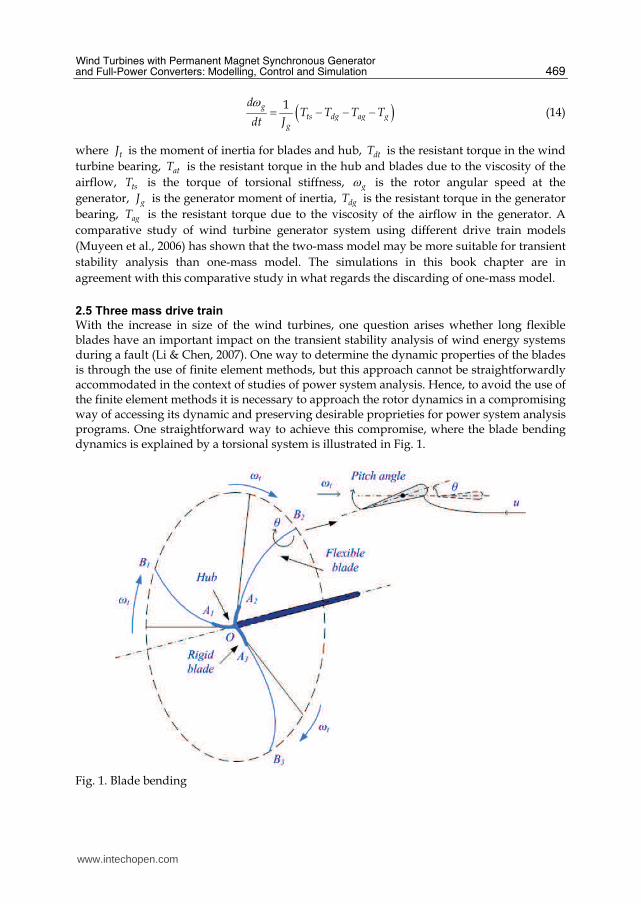
2.5 Three mass drive train
With the increase in size of the wind turbines, one question arises whether long flexible blades have an important impact on the transient stability analysis of wind energy systems during a fault (Li & Chen, 2007). One way to determine the dynamic properties of the blades is through the use of finite element methods, but this approach cannot be straightforwardly accommodated in the context of studies of power system analysis. Hence, to avoid the use of the finite element methods it is necessary to approach the rotor dynamics in a compromising way of accessing its dynamic and preserving desirable proprieties for power system analysis programs. One straightforward way to achieve this compromise, where the blade bending dynamics is explained by a torsional system is illustrated in Fig. 1.
Fig. 1. Blade bending
www.intechopen.com
Wind Turbines
470
Since the blade bending occurs at a significant distance from the joint between the blades and the hub, it is admissible to model the blades by splitting the blades in two parts: type OA parts, blade sections OA1, OA2 and OA3; and type AB parts, blade sections A1B1, A2B2 and A3B3. Type OA parts have an equivalent moment of inertia associated with the inertia of the hub and the rigid blade sections. Type OB parts have an equivalent moment of inertia associated with the inertia of the rest of the blade sections. Type OB parts are the effective flexible blade sections and are considered by the moment of inertia of the flexible blade sections. Type OA and OB parts are joined by the interaction of a torsional element, but in addition a second torsional element connecting the rest of the inertia presented in the angular movement of the rotor is needed, i.e., it is necessary to consider the moment of inertia associated with the rest of the mechanical parts, mainly due to the inertia of the generator. Hence, the configuration of this model is of the type shown in Fig. 2.
Fig. 2. Three-mass drive train model
The equations for the three-mass model are also based on the torsional version of the second law of Newton, given by
1
( )tt db bs
b
dT T T
dt J
ω = − − (15)
1
( )hbs dh ss
h
dT T T
dt J
ω = − − (16)
1
( )g
ss dg gg
dT T T
dt J
ω = − − (17)
where bJ is the moment of inertia of the flexible blades section , dbT is the resistant torque
of the flexible blades, bsT is the torsional flexible blades stifness torque, hω is the rotor
angular speed at the rigid blades and the hub of the wind turbine, hJ is the moment of
www.intechopen.com
Wind Turbines with Permanent Magnet Synchronous Generator and Full-Power Converters: Modelling, Control and Simulation
471
inertia of the hub and the rigid blades section, dhT is the resistant torque of the rigid blades
and the hub, ssT is the torsional shaft stifness torque, dgT is the resistant torque of the
generator. The moments of inertia for the model are given as input data, but in their absence
an estimation of the moments of inertia is possible (Ramtharan & Jenkins, 2007).
2.6 Generator
The generator considered in this book chapter is a PMSG. The equations for modelling a PMSG, using the motor machine convention (Ong, 1998), are given by
1
[ ]dd g q q d d
d
diu p L i R i
dt Lω= + − (18)
1
[ ( ) ]q
q g d d f q qq
diu p L i M i R i
dt Lω= − + − (19)
where di , qi are the stator currents, du , qu are the stator voltages, p is the number of pairs
of poles, dL , qL are the stator inductances, dR , qR are the stator resistances, M is the
mutual inductance, fi is the equivalent rotor current. In order to avoid demagnetization of
permanent magnet in the PMSG, a null stator current associated with the direct axis is
imposed (Senjyu et al., 2003).
2.7 Two-level converter
The two-level converter is an AC-DC-AC converter, with six unidirectional commanded
insulated gate bipolar transistors (IGBTs) used as a rectifier, and with the same number of
unidirectional commanded IGBTs used as an inverter. There are two IGBTs identified by i,
respectively with i equal to 1 and 2, linked to the same phase. Each group of two IGBTs
linked to the same phase constitute a leg k of the converter. Therefore, each IGBT can be
uniquely identified by the order pair (i, k). The logic conduction state of an IGBT identified
by (i, k) is indicated by ikS . The rectifier is connected between the PMSG and a capacitor
bank. The inverter is connected between this capacitor bank and a second order filter, which
in turn is connected to the electric network. The configuration of the simulated wind energy
conversion system with two-level converter is shown in Fig. 3.
Fig. 3. Wind energy conversion system using a two-level converter
www.intechopen.com
Wind Turbines
472
For the switching function of each IGBT, the switching variable kγ is used to identify the
state of the IGBT i in the leg k of the converter. Respectively, the index k with {1,2,3}k∈
identifies a leg for the rectifier and {4,5,6}k∈ identifies leg for the inverter. The switching
variable a leg in function of the logical conduction states (Rojas et al., 1995) is given by
and
and
1 2
1 2
1, ( 1 0)
0, ( 0 1)k k
kk k
S S
S Sγ = =⎧= ⎨ = =⎩ {1, ... ,6}k∈ (20)
but logical conduction states are constrained by the topological restrictions given by
2
1
1iki
S=
=∑ {1, ... ,6}k∈ (21)
Each switching variable depends on the conducting and blocking states of the IGBTs. The
voltage dcv is modelled by the state equation given by
3 6
1 4
1( )dc
k k k kk k
dvi i
dt Cγ γ
= == −∑ ∑ (22)
Hence, the two-level converter is modelled by (20) to (22).
2.8 Multilevel converter
The multilevel converter is an AC-DC-AC converter, with twelve unidirectional commanded IGBTs used as a rectifier, and with the same number of unidirectional commanded IGBTs used as an inverter.
The rectifier is connected between the PMSG and a capacitor bank. The inverter is connected
between this capacitor bank and a second order filter, which in turn is connected to an
electric network. The groups of four IGBTs linked to the same phase constitute a leg k of the
converter. The index i with {1,2,3,4}i∈ identifies a IGBT in leg k. As in the two-level
converter modelling the logic conduction state of an IGBT identified by the pair (i, k) is
indicated by ikS . The configuration of the simulated wind energy conversion system with
multilevel converter is shown in Fig. 4.
Fig. 4. Wind energy conversion system using a multilevel converter
www.intechopen.com
Wind Turbines with Permanent Magnet Synchronous Generator and Full-Power Converters: Modelling, Control and Simulation
473
For the switching function of each IGBT, the switching variable kγ is used to identify the
state of the IGBT i in the leg k of the converter. The index k with {1,2,3}k∈ identifies the
leg for the rectifier and {4,5,6}k∈ identifies the inverter one. The switching variable of each
leg k (Rojas et al., 1995) are given by
and and or
and and or
and and or
1 2 3 4
2 3 1 4
3 4 1 2
1,( ) 1 ( ) 0
0,( ) 1 ( ) 0
1,( ) 1 ( ) 0
k k k k
k k k k k
k k k k
S S S S
S S S S
S S S S
γ= =⎧⎪= = =⎨⎪− = =⎩
{1, ... ,6}k∈ (23)
constrained by the topological restrictions given by
1 2 2 3 3 4( . ) ( . ) ( . ) 1k k k k k kS S S S S S+ + = {1, ... ,6}k∈ (24)
With the two upper IGBTs in each leg k ( 1kS and 2kS ) of the converters it is associated a
switching variable 1kΦ and also with the two lower IGBTs ( 3kS and 4kS ) it is associated a
switching variable 2kΦ , respectively given by
1
(1 )
2k k
k
γ γ+Φ = ; 2
(1 )
2k k
k
γ γ−Φ = {1, ... ,6}k∈ (25)
The voltage dcv is the sum of the voltages 1Cv and 2Cv in the capacitor banks 1C and 2C ,
modelled by the state equation
3 6
1 11 1 4
3 6
2 22 1 4
1( )
1 ( )
dck k k k
k k
k k k kk k
dvi i
dt C
i iC
= =
= =
= Φ − Φ ++ Φ − Φ
∑ ∑∑ ∑ (26)
Hence, the multilevel converter is modelled by (23) to (26).
2.9 Matrix converter
The matrix converter is an AC-AC converter, with nine bidirectional commanded insulated
gate bipolar transistors (IGBTs). The logic conduction state of an IGBT is indicated by Sij.
The matrix converter is connected between a first order filter and a second order filter. The
first order filter is connected to a PMSG, while the second order filter is connected to an
electric network. The configuration of the simulated wind energy conversion system with
matrix converter is shown in Fig. 5.
The IGBTs commands ijS are function of the on and off states, given by
on
off
1, ( )
0,( )ijS⎧= ⎨⎩ , {1, 2, 3}i j∈ (27)
For the matrix converter modelling, the following restrictions are considered
www.intechopen.com
Wind Turbines
474
Fig. 5. Wind energy conversion system using a matrix converter
3
1
1ijj
S=
=∑ {1, 2, 3}i∈ (28)
3
1
1iji
S=
=∑ {1, 2, 3}j∈ (29)
The vector of output phase voltages is related to the vector of input phase voltages through the command matrix. The vector of output phase voltages (Alesina & Venturini, 1981) is given by
The vector of input phase currents is related to the vector of output phase currents through the command matrix. The vector of input phase currents is given by
[ ] [ ] [ ]T T Ta b c A B Ci i i S i i i= (31)
where
4 5 6[ ] [ ]a b ci i i i i i= (32)
4 5 6[ ] [ ]a b cv v v v v v= (33)
Hence, the matrix converter is modelled by (27) to (33). A switching strategy can be chosen
so that the output voltages have the most achievable sinusoidal waveform at the desired
frequency, magnitude and phase angle, and the input currents are nearly sinusoidal as
possible at the desired displacement power factor (Alesina & Ventirini, 1981). But, in general
terms it can be said that due to the absence of an energy storage element, the matrix
converter is particular sensitive to the appearance of malfunctions (Cruz & Ferreira, 2009).
www.intechopen.com
Wind Turbines with Permanent Magnet Synchronous Generator and Full-Power Converters: Modelling, Control and Simulation
475
2.10 Electric network
A three-phase active symmetrical circuit given by a series of a resistance and an inductance with a voltage source models the electric network. The phase currents injected in the electric network are modelled by the state equation given by
1( )
fkfk n fk k
n
diu R i u
dt L= − − {4,5,6}k = (34)
where nR and nL are the resistance and the inductance of the electric network, respectively,
fku is the voltage at the filter and ku is the voltage source for the simulation of the electric
network.
3. Control strategy
3.1 Fractional order controllers
A control strategy based on fractional-order PIμ controllers is considered for the variable-speed operation of wind turbines with PMSG/full-power converter topology. Fractional-order controllers are based on fractional calculus theory, which is a generalization of ordinary differentiation and integration to arbitrary non-integer order (Podlubny, 1999). Applications of fractional calculus theory in practical control field have increased significantly (Li & Hori, 2007), regarding mainly on linear systems (Çelik & Demir, 2010).
The design of a control strategy based on fractional-order PIμ controllers is more complex
than that of classical PI controllers, but the use of fractional-order PIμ controllers can improve properties and controlling abilities (Jun-Yi et al., 2006)-(Arijit et al., 2009). Different design methods have been reported including pole distribution, frequency domain approach, state-space design, and two-stage or hybrid approach which uses conventional integer order design method of the controller and then improves performance of the designed control system by adding proper fractional order controller. An alternative design method used is based on a particle swarm optimization (PSO) algorithm and employment of a novel cost function, which offers flexible control over time domain and frequency domain specifications (Zamani et al., 2009). Although applications and design methods regard mainly on linear systems, it is possible to use some of the knowledge already attained to envisage it on nonlinear systems, since the performance of fractional-order controllers in the presence of nonlinearity is of great practical interest (Barbosa et al., 2007). In order to examine the ability of fractional-order controllers for the variable-speed operation of wind turbines, this book chapter follows the tuning rules in (Maione & Lino, 2007). But, a more systematic procedure for controllers design needs further research in order to well develop tuning implementation techniques (Chen et al., 2009) for a ubiquitous use of fractional-order controllers.
The fractional-order differentiator denoted by the operator a tDμ (Calderón et al., 2006) is
given by
,( ) 0
1, ( ) 0
( ) 0( ) ,
a t
t
a
d
dtD
d
μμ
μμ
μμμτ −
⎧⎪ ℜ >⎪⎪= ℜ =⎨⎪ ℜ <⎪⎪⎩∫ (35)
www.intechopen.com
Wind Turbines
476
where μ is the order of derivative or integral, which can be a complex number, and ( )μℜ is
the real part of the μ . The mathematical definition of fractional derivative and integral has
been the subject of several approaches. The most frequently encountered one is the
Riemann–Liouville definition, in which the fractional-order integral is given by
Γ
11( ) ( ) ( )
( )
t
a t aD f t t f dμ μτ τ τμ− −= −∫ (36)
while the definition of fractional-order derivative is given by
Γ 1
( )1( )
( ) ( )
nt
a t n na
fdD f t d
n dt t
μ μτ τμ τ − +
⎡ ⎤= ⎢ ⎥− −⎢ ⎥⎣ ⎦∫ (37)
where
Γ 1
0( ) yxx y e dy
∞ −−≡ ∫ (38)
is the Euler’s Gamma function, a and t are the limits of the operation, and μ identifies the
fractional order. In this book chapter, μ is assumed as a real number that for the fractional
order controller satisfies the restrictions 0 1μ< < . Normally, it is assumed that 0a = . In
what follows, the following convention is used 0 t tD Dμ μ− −≡ . The other approach is
Grünwald–Letnikov definition of fractional-order integral given by
0
0
( )( ) lim ( )
! ( )h
t a
h
tr
rD f t h f t r h
rμ μ μ
μ→
−−
=Γ += −Γ∑ (39)
while the definition of fractional-order derivative is given by
0
0
( ) lim ( 1) ( )h
nh t a
n
tr
D f t h f t r hμ μ μ→≈ −
−=
= − −∑ (40)
An important property revealed by the Riemann–Liouville and Grünwald–Letnikov
definitions is that while integer-order operators imply finite series, the fractional-order
counterparts are defined by infinite series (Calderón et al., 2006), (Arijit et al., 2009). This
means that integer operators are local operators in opposition with the fractional operators
that have, implicitly, a memory of the past events. The differential equation for the
fractional-order PIμ controller 0 1μ< < is given by
( ) ( ) ( )p i tu t K e t K D e tμ−= + (41)
where pK is the proportional constant and iK is the integration constant. Taking 1μ = in
(41) a classical PI controller is obtained. The fractional-order PIμ controller is more flexible
than the classical PI controller, because it has one more adjustable parameter, which
reflects the intensity of integration. The transfer function of the fractional-order PIμ
controller, using the Laplace transform on (41), is given by
www.intechopen.com
Wind Turbines with Permanent Magnet Synchronous Generator and Full-Power Converters: Modelling, Control and Simulation
477
( ) p iG s K K s μ−= + (42)
A good trade-off between robustness and dynamic performance, presented in (Maione & Lino, 2007), is in favour of a value for μ in the range [0.4, 0.6].
3.2 Converters control
Power electronic converters are variable structure systems, because of the on/off switching of their IGBTs. Pulse width modulation (PWM) by space vector modulation (SVM) associated with sliding mode (SM) is used for controlling the converters. The sliding mode control strategy presents attractive features such as robustness to parametric uncertainties of the wind turbine and the generator, as well as to electric grid disturbances (Beltran et al., 2008). Sliding mode controllers are particularly interesting in systems with variable structure, such as switching power electronic converters, guaranteeing the choice of the most appropriate space vectors. Their aim is to let the system slide along a predefined sliding surface by changing the system structure. The power semiconductors present physical limitations that have to be considered during design phase and during simulation. Particularly, they cannot switch at infinite frequency. Also, for a finite value of the switching frequency, an error exists between the reference value and the control value. In order to guarantee that the system slides along the sliding surface, it has been proven that it is necessary to ensure that the state trajectory near the surfaces verifies the stability conditions (Rojas et al., 1995) given by
( , )
( , ) 0dS e t
S e tdt
αβαβ < (43)
in practice a small error 0ε > for ( , )S e tαβ is allowed, due to power semiconductors
switching only at finite frequency. Consequently, a switching strategy has to be considered
given by
( , )S e tαβε ε− < < + (44)
A practical implementation of this switching strategy at the simulation level could be
accomplished by using hysteresis comparators. The output voltages of matrix converter are
switched discontinuous variables. If high enough switching frequencies are considered, it is
possible to assume that in each switching period sT the average value of the output voltages
is nearly equal to their reference average value. Hence, it is assumed that
( 1) *1 s
s
n T
nTs
v dt vT
αβ αβ+ =∫ (45)
Similar to the average value of the output voltages, the average value of the input current is nearly equal to their reference average value. Hence, it is assumed that
( 1) *1 s
s
n T
q qnTs
i dt iT
+ =∫ (46)
The output voltage vectors in the α β plane for the two-level converter are shown in Fig. 6.
www.intechopen.com
Wind Turbines
478
Fig. 6. Output voltage vectors for the two-level converter
Also, the integer variables αβσ for the two-level converter take the values
αβσ with { }, 1,0,1α βσ σ ∈ − (47)
The output voltage vectors in the α β plane for the multilevel converter are shown in Fig. 7.
Fig. 7. Output voltage vectors for the two-level converter
The integer variables αβσ for the multilevel converter take the values
αβσ with { }, 2, 1, 0, 1, 2α βσ σ ∈ − − (48)
If 1 2C Cv v≠ , then a new vector is selected. The output voltage vectors and the input current
vectors in the α β plane for the matrix converter are shown respectively in Fig. 8 and Fig. 9.
Fig. 8. Output voltage vectors for the matrix converter
www.intechopen.com
Wind Turbines with Permanent Magnet Synchronous Generator and Full-Power Converters: Modelling, Control and Simulation
479
Fig. 9. Input current vectors for the matrix converter
The outputs of the hysteresis comparators are integer variables (Melício et al., 2010a). The
voltage integer variables αβσ for the matrix converter take the values
αβσ with { }, 1,0,1α βσ σ ∈ − (49)
The current integer variables qσ for the matrix converter in dq coordinates take the values
{ }1,1qσ ∈ − (50)
Hence, the proposed control strategy for the power electronic converters is given by the
consideration of (43) to (50). Design of PIμ controllers on the wind energy conversion
systems is made over the respective configurations. The design of PIμ controllers follows
the tuning rules in (Maione & Lino, 2007). Power electronic converters are modelled as a
pure delay (Chinchilla et al., 2006) and the left-over dynamics are modelled with a second
order equivalent transfer function, following the identification of a step response.
4. Power quality evaluation
The harmonic behaviour computed by the Discrete Fourier Transform is given by
1
2
0
( ) ( )N
j k n N
n
X k e x nπ− −=
= ∑ for 0,..., 1k N= − (51)
where ( )x n is the input signal and ( )X k is a complex giving the amplitude and phase of the
different sinusoidal components of ( )x n . The total harmonic distortion THD is defined by
the expression given by
THD
502
2(%) 100H
H
F
X
X==∑
(52)
where HX is the root mean square (RMS) value of the non-fundamental H harmonic,
component of the signal, and FX is the RMS value of the fundamental component
harmonic. Standards such as IEEE-519 (Standard 519, 1992) impose limits for different order
harmonics and the THD. The limit is 5% for THD is considered in the IEEE-519 standard
and is used in this book chapter as a guideline for comparison purposes.
www.intechopen.com
Wind Turbines
480
5. Simulation results
Consider a wind power system with the moments of inertia of the drive train, the stiffness, the turbine rotor diameter, the tip speed, the rotor speed, and the generator rated power, given in Table 2.
Blades moment of inertia 400×10³ kgm²
Hub moment of inertia 19.2×10³ kgm²
Generator moment of inertia 16×10³ kgm²
Stiffness 1.8×10⁶ Nm
Turbine rotor diameter 49 m
Tip speed 17.64-81.04 m/s
Rotor speed 6.9-30.6 rpm
Generator rated power 900 kW
Table 2. Wind energy system data
The time horizon considered in the simulations is 5 s.
5.1 Pitch angle control malfunction
Consider a pitch angle control malfunction starting at 2 s and lengthen until 2.5 s due to a total cut-off on the capture of the energy from the wind by the blades (Melício et al., 2010b), and consider the model for the wind speed given by
( ) 15 1 sin( )k kk
u t A tω⎡ ⎤= +⎢ ⎥⎣ ⎦∑ 0 5t≤ ≤ (53)
This wind speed in function of the time is shown in Fig. 10.
Fig. 10. Wind speed
www.intechopen.com
Wind Turbines with Permanent Magnet Synchronous Generator and Full-Power Converters: Modelling, Control and Simulation
481
In this simulation after some tuning it is assumed that 0.5μ = . The mechanical power over
the rotor of the wind turbine disturbed by the mechanical eigenswings, and the electric power of the generator is shown in Fig. 11. Fig. 11 shows an admissible drop in the electrical power of the generator, while the mechanical power over the rotor is null due to the total cut-off on the capture of the energy from the wind by the blades. The power coefficient is shown in Fig. 12.
Fig. 11. Mechanical power over the rotor and electric power
Fig. 12. Power coefficient
The power coefficient is at the minimum value during the pitch control malfunction,
induced by the mistaken wind gust position. The voltage dcv for the two-level converter
with the fractional order controller, respectively for the three different mass drive train
models are shown in Fig. 13.
www.intechopen.com
Wind Turbines
482
Fig. 13. Voltage at the capacitor for two-level converter using a fractional-order controller
The voltage dcv for the two-level converter presents almost the same behaviour with the
two-mass or the three-mass models for the drive train. But one-mass model omits significant
dynamic response as seen in Fig. 13. Hence, as expected there is in this case an admissible
use for a two-mass model; one-mass model is not recommended in confining this behaviour.
Nevertheless, notice that: the three-mass model is capturing more information about the
behaviour of the mechanical drive train on the system. The increase on the electric power of
wind turbines, imposing the increase on the size of the rotor of wind turbines, with longer
flexible blades, is in favour of the three-mass modelling.
5.2 Converter control malfunction
Consider a wind speed given by
( ) 20 1 sin( )k kk
u t A tω⎡ ⎤= +⎢ ⎥⎣ ⎦∑ 0 5t≤ ≤ (54)
The converter control malfunction is assumed to occur between 2.00 s and 2.02 s, imposing a
momentary malfunction on the vector selection for the inverter of the two-level and the
multilevel converters and on the vector selection for the matrix converter. This malfunction
is simulated by a random selection of vectors satisfying the constraint of no short circuits on
the converters. In this simulation after some tuning it was assumed 0.7μ = . Simulations
with the model for the matrix converter were carried out, considering one-mass, two-mass
and three-mass drive train models in order to establish a comparative behaviour (Melício et
al., 2010c). The mechanical torque over the rotor of the wind turbine disturbed by the mechanical
eigenswings and the electric torque of the generator, with the one-mass, two-mass and
three-mass drive train models, are shown in Figs. 14, 15 and 16, respectively. As shown in
these figures, the electric torque of the generator follows the rotor speed at the PMSG, except
when it is decreased due to the malfunction. For the same fault conditions, the transient
www.intechopen.com
Wind Turbines with Permanent Magnet Synchronous Generator and Full-Power Converters: Modelling, Control and Simulation
483
response of the three-mass drive train model is significantly different than that of the two-
mass model, since it captures more information about the behaviour of the system. The
results have shown that the consideration of the bending flexibility of blades influences the
wind turbine response during internal faults (Melício et al., 2010d).
The voltage dcv for the two-level and the multilevel converters with a three-mass drive train
model is shown in Fig. 17. As expected during the malfunction this voltage suffers a small increase, the capacitor is charging, but almost after the end of the malfunction voltage recovers to its normal value (Melício et al., 2010e).
Fig. 14. Mechanical and electric torque with the one-mass drive train model and using a matrix converter
Fig. 15. Mechanical and electric torque with the two-mass drive train model and using a matrix converter
www.intechopen.com
Wind Turbines
484
Fig. 16. Mechanical and electric torque with the three-mass drive train model and using a matrix converter
Fig. 17. Voltage dcv for the two-level and the multilevel converter using a three-mass drive
train model The currents injected into the electric grid by the wind energy system with the two-level converter and a three-mass drive train model are shown in Fig. 18. The currents injected into the electric grid for the wind energy system with a multilevel converter and a three-mass drive train model are shown in Fig. 19. The currents injected into the electric grid for the wind energy system with matrix converter and a three-mass drive train model are shown in Fig. 20.
www.intechopen.com
Wind Turbines with Permanent Magnet Synchronous Generator and Full-Power Converters: Modelling, Control and Simulation
485
Fig. 18. Currents injected into the electric grid (two-level converter and a three-mass drive train model)
Fig. 19. Currents injected into the electric grid (multilevel converter and three-mass drive train model)
www.intechopen.com
Wind Turbines
486
Fig. 20. Currents injected into the electric grid (matrix converter and three-mass drive train model)
As shown in Figs. 18, 19 or 20, during the malfunction the current decreases, but almost after the end of the malfunction the current recovers its normal behaviour.
5.3 Harmonic assessment considering ideal sinusoidal voltage on the network
Consider the network modelled as a three-phase active symmetrical circuit in series, with
850 V at 50 Hz. In the simulation after some tuning it is assumed that 0.5μ = . Consider the
wind speed in steady-state ranging from 5-25 m/s. The goal of the simulation is to assess the third harmonic and the THD of the output current. The wind energy conversion system using a two-level converter in steady-state has the third harmonic of the output current shown in Fig. 21, and the THD of the output current shown in Fig. 22. The wind energy conversion system with multilevel converter in steady-state has
Fig. 21. Third harmonic of the output current, two-level converter
www.intechopen.com
Wind Turbines with Permanent Magnet Synchronous Generator and Full-Power Converters: Modelling, Control and Simulation
487
the third harmonic of the output current shown in Fig. 23, and the THD of the output current shown in Fig. 24. The wind energy conversion system with matrix converter in steady-state has the third harmonic of the output current shown in Fig. 25, and the THD of the output current shown in Fig. 26. The fractional-order control strategy provides better results comparatively to a classical integer-order control strategy, in what regards the third harmonic of the output current and the THD.
Fig. 22. THD of the output current, two-level converter
Fig. 23. Third harmonic of the output current, multilevel converter
www.intechopen.com
Wind Turbines
488
Fig. 24. THD of the output current, multilevel converter
Fig. 25. Third harmonic of the output current, matrix converter
www.intechopen.com
Wind Turbines with Permanent Magnet Synchronous Generator and Full-Power Converters: Modelling, Control and Simulation
489
Fig. 26. THD of the output current, matrix converter
5.4 Harmonic assessment considering non-ideal sinusoidal voltage on the network
Consider the network modelled as a three-phase active symmetrical circuit in series, with
850 V at 50 Hz and 5 % of third harmonic component. In this simulation after some tuning it
is assumed that 0.5μ = . Consider the wind speed in steady-state ranging from 5-25 m/s. The wind energy conversion system using a two-level converter in steady-state has the third harmonic of the output current shown in Fig. 27, and the THD of the output current shown in Fig. 28. The wind energy conversion system with multilevel converter in steady-state has the third harmonic of the output current shown in Fig. 29, and the THD of the output current shown in Fig. 30. The wind energy conversion system with matrix converter in steady-state has the third harmonic of the output current shown in Fig. 31, and the THD of the output current shown in Fig. 32.
Fig. 27. Third harmonic of the output current, two-level converter
www.intechopen.com
Wind Turbines
490
Fig. 28. THD of the output current, two-level converter
Fig. 29. Third harmonic of the output current, multilevel converter
www.intechopen.com
Wind Turbines with Permanent Magnet Synchronous Generator and Full-Power Converters: Modelling, Control and Simulation
491
Fig. 30. THD of the output current, multilevel converter
Fig. 31. Third harmonic of the output current, matrix converter
www.intechopen.com
Wind Turbines
492
Fig. 32. THD of the output current, matrix converter
The THD of the current injected into the network is lower than the 5% limit imposed by
IEEE-519 standard for the two-level and multilevel converters, and almost near to this limit
for the matrix converter.
The fact that a non-ideal sinusoidal voltage on the network has an effect on the current THD of
the converters can be observed by comparison of Fig. 21 until Fig. 26 with Fig. 27 until Fig. 32.
Also, from those figures it is possible to conclude that the fractional-order controller
simulated for the variable-speed operation of wind turbines equipped with a PMSG has
shown an improvement on the power quality in comparison with a classical integer-order
control strategy, in what regards the third harmonic of the output current and the THD.
6. Conclusion
The assessment of the models ability to predict the behaviour for the drive train is in favour
of the two-mass model or the three-mass model for wind energy conversion systems with
electric power in the range of the values used in the simulations.
But, with the increase on the electric power of wind turbines, imposing the increase on the size
of the rotor of wind turbines, with longer flexible blades, the study on the transient stability
analysis of wind energy conversion systems will show a favour for a three-mass modelling.
The fractional-order controller simulated for the variable-speed operation of wind turbines
equipped with a PMSG has shown an improvement on the power quality in comparison
with a classical integer-order control strategy, in what regards the level for the third
harmonic on the output current and the THD.
Accordingly, it is shown that the THD of the current for the wind energy conversion system
with either a two-level or a multilevel converter is lower than with a matrix converter.
Finally, the results have shown that the distortion on the voltage of the electric network due
to the third harmonic influences significantly the converter output electric current.
Particularly, in what concerns to the use of the two-level, multilevel and matrix converters
the last one can be the first to be out of the 5% limit imposed by IEEE-519 standard, if a
major harmonic content on the voltage of the electric network is to be considered.
www.intechopen.com
Wind Turbines with Permanent Magnet Synchronous Generator and Full-Power Converters: Modelling, Control and Simulation
493
7. References
Akhmatov, V.; Knudsen, H. & Nielsen, A. H. (2000). Advanced simulation of windmills in the electric power supply. Int. J. Electr. Power Energy Syst., Vol. 22, No. 6, August 2000, pp. 421-434, ISSN: 0142-0615.
Alesina, A. & Venturini, M. (2000). Solid-state power conversion: a Fourier analysis approach to generalized transformer synthesis. IEEE Trans. Circuits Syst., Vol. 28, No. 4, April 1981, pp. 319-330, ISSN: 0098-4094.
Arijit, B.; Swagatam, D.; Ajith, A. & Sambarta, D. (2009). Design of fractional-order PI-lambda-D-mu-controllers with an improved differential evolution. Eng. Appl. Artif. Intell., Vol. 22, No. 2, March 2009, pp. 343-350, ISSN: 0952-1976.
Barbosa, R. S.; Machado, J. A. T. & Galhano, M. (2007). Performance of fractional PID algorithms controlling nonlinear systems with saturation and backlash phenomena. J. Vibration and Control, Vol. 13, No. 9-10, September 2007, pp. 1407-1418, ISSN: 1077-5463.
Beltran, B.; Ahmed-Ali, T. & Benbouzid, M. E. H. (2008). Sliding mode power control of variable-speed wind energy conversion systems. IEEE Trans. Energy Convers., Vol. 23, No. 2, June 2008, pp. 551-558, ISSN: 0885-8969.
Calderón, A. J.; Vinagre, B. M. & Feliu, V. (2006). Fractional order control strategies for power electronic buck converters. Signal Processing, Vol. 86, No. 10, October 2006, pp. 2803-2819, ISSN: 0165-1684.
Chen, Y. Q.; Petráš, I. & Xue, D. (2009). Fractional order control–a tutorial, Proceedings of 2009 American Control Conference, pp. 1397-1411, ISBN: 978-1-4244-4523-3, USA, June 2009, St. Louis.
Chen, Z. & Spooner, E. (2001). Grid power quality with variable speed wind turbines. IEEE Trans. Energy Convers., Vol. 16, No. 2, (June 2001) pp. 148-154, ISSN: 0885-8969.
Çelik, V. & Demir, Y. (2010). Effects on the chaotic system of fractional order PI-alfa controller. Nonlinear Dynamics, Vol. 59, No. 1-2, January 2010, pp. 143-159, ISSN: 0924-090X.
Chinchilla, M.; Arnaltes, S. & Burgos, J. C. (2006). Control of permanent-magnet generators applied to variable-speed wind energy systems connected to the grid. IEEE Trans. Energy Convers., Vol. 21, No. 1, March 2006, pp. 130-135, ISSN: 0885-8969.
Cruz, S. M. A. & Ferreira, M. (2009). Comparison between back-to-back and matrix converter drives under faulty conditions, Proceedings of EPE 2009, pp. 1-10, ISBN: 978-1-4244-4432-8, Barcelona, September 2009, Spain.
Jun-Yi, C. & Bing-Gang, C. (2006). Design of fractional order controllers based on particle swarm, Proceedings of IEEE ICIEA 2006, pp. 1-6, ISBN: 0-7803-9514-X, Malaysia, May 2006, Singapore.
Li, H. & Chen, Z. (2007). Transient stability analysis of wind turbines with induction generators considering blades and shaft flexibility, Proceedings of 33rd IEEE IECON 2007, pp. 1604-1609, ISBN: 1-4244-0783-4, Taiwan, November 2007, Taipei.
Li, W. & Hori, Y. (2007). Vibration suppression using single neuron-based PI fuzzy controller and fractional-order disturbance observer. IEEE Trans. Ind. Electron., Vol. 54, No. 1, February 2007, pp. 117-126, ISSN: 0278-0046.
Maione, G. & Lino, P. (2007). New tuning rules for fractional PI-alfa controllers. Nonlinear Dynamics, Vol. 49, No. 1-2, July 2007, pp. 251-257, ISSN: 0924-090X.
Melício, R.; Mendes, V. M. F. & Catalão, J. P. S. (2010a). Modeling, control and simulation of full-power converter wind turbines equipped with permanent magnet synchronous generator. International Review of Electrical Engineering, Vol. 5, No. 2, March-April 2010, pp. 397-408, ISSN: 1827-6660.
www.intechopen.com
Wind Turbines
494
Melício, R.; Mendes, V. M. F. & Catalão, J. P. S. (2010b). A pitch control malfunction analysis for wind turbines with permanent magnet synchronous generator and full-power converters: proportional integral versus fractional-order controllers. Electric Power Components and Systems, Vol. 38, No. 4, 2010, pp. 387-406, ISSN: 1532-5008.
Melício, R.; Mendes, V. M. F. & Catalão, J. P. S. (2010c). Wind turbines equipped with fractional-order controllers: stress on the mechanical drive train due to a converter control malfunction. Wind Energy, 2010, in press, DOI: 10.1002/we.399, ISSN: 1095-4244.
Melício, R.; Mendes, V. M. F. & Catalão, J. P. S. (2010d). Harmonic assessment of variable-speed wind turbines considering a converter control malfunction. IET Renewable Power Generation, Vol. 4, No. 2, 2010, pp. 139-152, ISSN: 1752-1416.
Melício, R.; Mendes, V. M. F. & Catalão, J. P. S. (2010e). Fractional-order control and simulation of wind energy systems with PMSG/full-power converter topology. Energy Conversion and Management, Vol. 51, No. 6, June 2010, pp. 1250-1258, ISSN: 0196-8904.
Muyeen, S. M.; Hassan Ali, M.; Takahashi, R.; Murata, T.; Tamura, J.; Tomaki, Y.; Sakahara, A. & Sasano, E. (2006). Transient stability analysis of grid connected wind turbine generator system considering multi-mass shaft modeling. Electr. Power Compon. Syst., Vol. 34, No. 10, October 2006, pp. 1121-1138, ISSN: 1532-5016.
Ong, P.-M. (1998). Dynamic Simulation of Electric Machinery: Using Matlab/Simulink, Prentice-Hall, ISBN: 0137237855, New Jersey.
Podlubny, I. (1999). Fractional-order systems and PI-lambda-D-mu-controllers. IEEE Trans. Autom. Control, Vol. 44, No. 1, January 1999, pp. 208-214, ISSN: 0018-9286.
Ramtharan, G. & Jenkins, N. (2007). Influence of rotor structural dynamics representations on the electrical transient performance of DFIG wind turbines. Wind Energy, Vol. 10, No. 4, (March 2007) pp. 293-301, ISSN: 1095-4244.
Rojas, R.; Ohnishi, T. & Suzuki, T. (1995). Neutral-point-clamped inverter with improved voltage waveform and control range. IEEE Trans. Industrial Elect., Vol. 42, No. 6, (December 1995) pp. 587-594, ISSN: 0278-0046.
Salman, S. K. & Teo, A. L. J. (2003). Windmill modeling consideration and factors influencing the stability of a grid-connected wind power-based embedded generator. IEEE Trans. Power Syst., Vol. 16, No. 2, (May 2003) pp. 793-802, ISSN: 0885-8950.
Senjyu, T.; Tamaki, S.; Urasaki, N. & Uezato, K. (2003). Wind velocity and position sensorless operation for PMSG wind generator, Proceedings of 5th Int. Conference on Power Electronics and Drive Systems 2003, pp. 787-792, ISBN: 0-7803-7885-7, Malaysia, January 2003, Singapore.
Slootweg, J. G.; de Haan, S. W. H.; Polinder, H. & Kling, W. L. (2003). General model for representing variable speed wind turbines in power system dynamics simulations. IEEE Trans. Power Syst., Vol. 18, No. 1, February 2003, pp. 144-151, ISSN: 0885-8950.
Standard 519 (1992). [52] IEEE Guide for Harmonic Control and Reactive Compensation of Static Power Converters, IEEE Standard 519-1992.
Timbus, A.; Lisserre, M.; Teodorescu, R.; Rodriguez, P. & Blaabjerg, F. (2009). Evaluation of current controllers for distributed power generation systems. IEEE Trans. Power Electron., Vol. 24, No. 3, March 2009, pp. 654-664, ISSN: 0885-8993.
Xing, Z. X.; Zheng, Q. L.; Yao, X. J. & Jing, Y. J. (2005). Integration of large doubly-fed wind power generator system into grid, Proceedings of 8th Int. Conf. Electrical Machines and Systems, pp. 1000-1004, ISBN: 7-5062-7407-8, China, September 2005, Nanjing.
Zamani, M.; Karimi-Ghartemani, M.; Sadati, N. & Parniani, M. (2009). Design of fractional order PID controller for an AVR using particle swarm optimization. Control Eng. Practice, Vol. 17, No. 12, December 2009, pp. 1380-1387, ISSN: 0967-0661.
www.intechopen.com
Wind TurbinesEdited by Dr. Ibrahim Al-Bahadly
ISBN 978-953-307-221-0Hard cover, 652 pagesPublisher InTechPublished online 04, April, 2011Published in print edition April, 2011
InTech ChinaUnit 405, Office Block, Hotel Equatorial Shanghai No.65, Yan An Road (West), Shanghai, 200040, China
Phone: +86-21-62489820 Fax: +86-21-62489821
The area of wind energy is a rapidly evolving field and an intensive research and development has taken placein the last few years. Therefore, this book aims to provide an up-to-date comprehensive overview of thecurrent status in the field to the research community. The research works presented in this book are dividedinto three main groups. The first group deals with the different types and design of the wind mills aiming forefficient, reliable and cost effective solutions. The second group deals with works tackling the use of differenttypes of generators for wind energy. The third group is focusing on improvement in the area of control. Eachchapter of the book offers detailed information on the related area of its research with the main objectives ofthe works carried out as well as providing a comprehensive list of references which should provide a richplatform of research to the field.
How to referenceIn order to correctly reference this scholarly work, feel free to copy and paste the following:
Rui Melício, Victor M. F. Mendes and João P. S. Catalão (2011). Wind Turbines with Permanent MagnetSynchronous Generator and Full-Power Converters: Modelling, Control and Simulation, Wind Turbines, Dr.Ibrahim Al-Bahadly (Ed.), ISBN: 978-953-307-221-0, InTech, Available from:http://www.intechopen.com/books/wind-turbines/wind-turbines-with-permanent-magnet-synchronous-generator-and-full-power-converters-modelling-contro