MISCELLANEOUS PAPER CERC-91-2 C,WIND-WAVE GENERATION

£ON RESTRICTED FETCHES

by

D-A237 420 Jane M. SmithD-A237 420 ,Coastal Engineering Research Center

DEPARTMENT OF THE ARMYWaterways Experiment Station, Corps of Engineers

3909 Halls Ferry Road, Vicksburg, Mississippi 39180-6199

DTIC.ELECTE 1/ _ T. JUL 0 3 1991 '

May 1991Final Report

Approved For Public Release; Distribution Unlimited

91-03927

GPrepared for DEPARTMENT OF THE ARMYA KUS Army Corps of Engineers

Washington, DC 20314-1000

Under Work Unit 31592• = _= 0 ,-', OK!

Destroy this report when no longer needed. Do not returnit to the originator.

The findings in this report are not to be construed as an officialDepartment of the Army position unless so designated

by other authorized documents.

The contents of this report are not to be used foradvertising, publication, or promotional purposes.

Citation of trade names does not constitute anofficial endorsement or approval of the use of

such commercial products.

Form Appioved

REPORT DOCUMENTATION PAGE OMB Ho. 0704-0188

P ~ ~ ~ ~ ~ ~ ~ ~ ~ ~ ~~~~~h 6 o .C-W .t~~ e ~A~ ~ ~ fal ;e-C amue ew=9 da:a Scxt

;Q A~C4j~~:~~ r areo-_ 3B c Dae.-or to &ctad -. s 12 's

1. AGENCY USE ONLY (Leave blank) 12. REPORT DATE -3. REPORT TYPE AND DATES COVERED

! May 1991 1 Final Report4. TITLE AND SUBTITLE S. FUNDING NUMBERS

Wind-Wave Generation on Restricted Fetches Work Unit 31592

6. AUTHORS)

Jane M. Smith

7. PERFORMING ORGANIZATION NAME(S) AND ADDRESS(ES) 8. PERFORMING ORGANIZATIONREPORT NUMBER

USAE Waterways Experiment Station, Miscellaneous PaperCoastal Engineering Research Center CERC-91-23909 Halls Ferry Road, Vicksburg, MS 39180-6199

9. SPONSORING/MONITORING AGENCY NAME(S) AND ADDRESS(ES) 10. SPONSORING/MONITORINGAGENCY REPORT NUMBER

I US Army Corps of EngineersWashington, DC 20314-1000

11. SUPPLEMENTARY NOTES

Available from National Technical Information Service, 5285 Port Royal Road, Springfield,VA 22161.

12a. DISTRIBUTION /AVAILABILITY STATEMENT 12b. DISTRIBUTION CODE

Approved for public release; distribution unlimited

13. ABSTRACT (Maximum 200 words)

Wind-wave generation in lakes, rivers, bays, and reservoirs is generally limited by the geometryof the water body, which is often very irregular. Most approaches to this problem consider wavegeneration only in the direction of the wind with fetch lengths averaged over small arcs of large arcs.Donelan proposed wave generation on fetch lengths in off-wind directions with reduced wind forcing(reduced by the cosine of the angle between the off-wind and wind directions) for the Great Lakes.The model described in this report, NARFET, is based on the Donelan concept, allowing wavegeneration in off-wind directions. Expressions are developed for significant wave height and peakperiod as a function of fetch geometry and wind speed based on linear regressions of wave datacollected on Puget Sound, Washington; Fort Peck Reservoir, Montana; Denison Reservoir, Texas;and Lake Ontario. The mean wave direction is determined by maximizing the wave period. Theequations differ from those given by Donelan, which were developed for the longer, more regular-shaped fetches of the Great Lakes. The NARFET model is quick and inexpensive (runs on aper-onal computer), yet conmider; the complexity of fetch geometry.

14. SUBJECT TERMS 15. NUMBER OF PAGESNarrow fetch Restricted fetch 51Reservoir waves Wind-wave generation 16. PRICE CODE

17. SECURiTy CLASSIFICATION 18. SECURITY CLASSIFICATION 119. SECURITY CLASSIFICATION 20. LIMITATION OF ABSTRACTOF REPC .r OF THIS PAGE OF ASTRACT

NCLASSIFIrN I UNCT ASSIFIED UNCLASSIFIED -(Rev_2-89)NSN: 7510-01-280-5500 Standard Form 2Q8 (Rev 2-89)

Pescribed by ANSI Std Z3 4,8298102

PREFACE

The investigation described in this report was authorized as a part of

the Civil Works Research and Development Program by Headquarters, US Army

Corps of Engineers (HQUSACE). Work was performed under Work Unit 31592, "Wave

Estimation for Design, Coastal Flooding Program," at the Coastal Engineering

Research Center (CERC), of the US Army Engineer Waterways Experiment Station

(WES). Messrs. John H. Lockhart, Jr., and John G. Housley were HQUSACE Tech-

nical Monitors. Dr. C. Linwood Vincent is the CERC Program Manager.

This study was conducted from July 1987 through May 1988 by Ms. Jane H.

Smith, Hydraulic Engineer, CERC. The study was done under the general super-

vision of Dr. James R. Houston and Mr. Charles C. Calhoun, Jr., Chief and

Assistant Chief, CERC, respectively; and under the direct supervision of

Mr. H. Lee Butler, Chief, Research Division; Dr. Edward F. Thompson, former

Chief, Coastal Oceanography Branch, and Dr. Robert E. Jensen, Principal Inves-

tigator, Wave Estimation for Design Work Unit, CERC. Dr. Steven A. Hughes,

Wave Dynamics Division, CERC, pcovided technical review of this report, and

Ms. Victoria L. Edwards, CERC, did word processing.

Commander and Director of WES during the publication of this report was

COL Larry B. Fulton, EN. Technical Director was Dr. Robert W. Whalin.

DII.

D!IC TA 0

Tii

I y

! -

CON~TENTS

Pa ge

PREFACE 1

PART I: INTRODUCTION. ......... ................. 3

Background. ......... .................... 3

Scope. .. .................. ............ 3

PART II: MODEL DEVELOPMENT .. ......... .............. 5

Previous Work .. ........ ................... 5Data. ......... ............... ......... 8Comparison of Models. .......... .............. 9Improved Model .. .................. ....... 14

PART III: MODE.. APPLICATION .. ...................... 19

Program Input. .. ................. ........ 19Program Output .. .................. ....... 22

PART IV: CONCLUSIONS .. .................... .... 24

REFERENCES. .......... ...................... 25

APPENDIX A: DATA .. ........ .................... Al

APPENDIX B: SAMPLE RUN. .. .................. ..... Bl

APPENDIX C: COMPUTER PROGRAM. .. ..................... Cl

APPENDIX D: NOTATION. .. ................. ....... Dl

2

WIND-WAJE GENERATION ON RESTRICTED FETCHES

PART I: INTRODUCTION

Background

1. Wind-wave generation in lakes, rivers, bays, and reservoirs is gen-

erally limited by the geometry of the water body, which is often very irregu-

lar. In the open ocean, wave generation is limited by the extent of the

meteorological disturbances, where the fetch widths are of the same order of

magnitude as the fetch lengths, and only the length, not the shape of the

fetch, is considered important. Although the effect of fetch length is fairly

well understood, the effect of fetch shape (especially for very irregular or

narrow fetches) has received only limited attention.

2. Fetch lengths for restricted fetches are normally measured from the

shoreline to the point of interest, in the direction of the wind. The Shore

Protection Manual (SPM) (1984) recommends applying this straight-line fetch

length to wave forecasting curves or equations, giving no consideration to the

fetch geometry. Other methods proposed for restricted fetch wave generation

consider fetch lengths in off-wind directions by applying weighting factors (a

function of the cosine of the angle between the off-wind and wind directions)

to the fetch lengths and averaging these weighted lengths over large arcs on

either side of the wind direction. These methods tend to reduce fetch lengths

through averaging. Another method, developed for the Great Lakes, considers

wave generation on fetch lengths in off-wind directions with a reduced wind

forcing (reduced by the cosine of the angle between the off-wind and wind

direction). This method has been successful on the Great Lakes, but has not

been tested for very irregular or narrow fetches. Complex numerical models of

wind-wave generation are also applicable to restricted fetches, but the ef-

fort, cost, and computer resources for the required resolution make them un-

economical for small projects.

Scope

3. The purpose of this report is to present the development and appli-

cation of the restricted fetch wind-wave generation model NARFET. Methods

3

developed in previous studies were reviewed and tested with field data. Based

on the strong points of the previous methods and the field data, an improved

model (NARFET) was developed. The model is quick and inexpensive, yet in-

cludes the complexity of fetch geometry not considered in the SPM method. The

model considers only constant, steady-state winds over the fetch. The effect

of depth is not included (most applications are in relatively deep water).

4

PART II: MODEL DEVELOPMENT

Previous Work

4. The first method used to account for the effect of fetch shape was

the effective fetch method proposed by Saville (1954). Saville assumed that

wind transfers energy to the water surface in the direction of the wind and in

all directions within 45 deg either side of the wind direction. For off-wind

directions, the amount of energy transferred is modified by the cosine of the

angle between the off-wind and wind directions. An effective fetch was deter-

mined and applied to wave forecasting curves or equations developed for unre-

stricted fetches (SPM 1966) to predict significant wave height and period or

energy spectrum. The effective fetch was defined as follows:

E Xi cos2

Feff = E cos 01 (1)

where

Feff = effective fetch*

Xi - length of the straight-line fetch

01 - angle from mean wind direction

Straight-line fetches were measured at increments of 6 deg over a 90-deg arc

(45 deg either side of the mean wind direction). This method usually predicts

lower wave heights and periods than when fetch shape is not considered. This

method was recommended by the SPM (1966). More recent SPM (1984) guidance

recommends using a simple fetch with the wave forecasting curves. The simple

fetch is determined by arithmetically averaging straight-line fetches at in-

crements of 3 deg over a 24-deg arc (12 deg either side of the mean wind di-

rection). This method is more conservative than the effective fetch method in

most cases, and it is easier to apply. Both these methods assume wave direc-

tion is coincident with wind direction, and the shape of the energy spectrum

is not affected by fetch shape.

5. Seymour (1977) argued that these two assumptions, wind and wave di-

rection coincident and spectral shape unaffected by fetch shape, were not

* For convenience, symbols are listed and defined in the Notation

(Appendix D).

5

valid. He suggested that both frequency and directional spread of the energy

spectrum would be broader for a restricted fetch than for the open ocean, so

he proposed the spectral contribution method. This method assumed a cosine-

squared direction distribution of wave energy over a 180-deg arc (90 deg

either side of the wind direction). The energy in a given spectral component

Si is given by:

Si(f,Oi,Fi) = 0.6366AOS(f,F i ) cos 2 o, (2)

where

Si - energy spectral component

f = frequency

Fi - fetch in 8i direction

AO = angle increment

S(f,Fi) - either the JONSWAP (Hasselmann et al. 1973) or Bretschneider(1963) energy spectrum

The spectrum is obtained by summing the energy in each frequency component

over all directions. This method is tedious, but it has the advantage of

considering fetch geometry as well as wind direction in estimating wave direc-

tion. This method tends to give lower wave heights and longer peak periods

than the effective fetch and simple fetch methods. The shape of the energy

spectrum is questionable because it does not account for smearing caused by

wave-wave interaction which tends to smooth the spectral shape to a similar

form.

6. The effective fetch, simple fetch, and spectral contribution methods

all allow the user to select the relationship of wave height and period to

fetch and wind speed. The equations derived from the JONSWAP experiment

(Hasselmann et al. 1973) are commonly used:

H - 0.0016g-0.5X0 .5U

(3)fp = 3.5gO.

67 X-0.3

3U-0.3 3

where

H - significant wave height

g = gravitational acceleration

X = fetch

6

U = wind speed

fp= peak frequency

Donelan (1980) developed slightly different relationships for H and fp

based on data collected in the Great Lakes:

H = 0.00366g-0 .62FO 38(U cos 4)1.24

(4)fp = 1.85g

0'77F-0.23(U cos 0)-0.54

where 4 is the angle between the wind and wave direction and F is the

straight-line fetch in the direction of the waves. He does not assume that

the wind and wave directions are the same, but for wave prediction, maximizes

the product:

(cos 4) 0. 54 F0 . 23 (5)

which is derived from maximizing the wave period (reciprocal of Equation 4).

This product is a function of fetch geometry. Donelan's approach can be sum-

marized as balancing a reduced wind forcing U cos (4) with increased fetch

distance in an off-wind direction. Donelan's model gives excellent results

for wave direction in Great Lakes experiments. The model has been criticized

by Walsh et al. (in preparation) because theoretical considerations suggest

that wave energy is a linear function of fetch, and therefore, wave height

should be a function of fetch to the 0.5 power (Rottier and Vincent 1982).

7. Walsh et al. use Donelan's basic model form and assume (a) an expo-

nent p in the cos (4) term to account for a reduced effectiveness of wind

in off-wind directions, (b) wave height is proportional to fetch to the 0.5

power, and (c) wave direction given by Donelan's model is correct, but both H

and T (period, l/fp ) should be maximized. With these assumptions, they

give the following expressions:

H = 0.0017F°'g-0 5U (cos 4)1.63

(6)fp = 2.3F-0 -29g0

71U °0 42 (cos 4)0.685

The models of both Donelan and Walsh et al. are easy to apply, but neither has

been tested for narrow, restricted fetches.

7

8. Sophisticated numerical finite-difference models of large-scale

wave generation have been developed in recent years (e.g., SHALWV model

(Hughes and Jensen 1986)) based on momentum transfer from the wind to the

waves. This type of model is applicable to wave generation on restricted

fetches, but requires small spatial grid cells and time steps to resolve the

fetch shape, making simulations expensive. Also, many of the complexities in

the models are normally not needed for restricted fetch applications

(spatially and temporally varying wind fields, swell propagation,

shallow-water effects).

Data

9. Limited wave data from four sources were compiled to test the mod-

els developed in the previous studies and to consider improved methods. The

sites include Denison Reservoir, Texas (two locations) (US Army Corps of Engi-

neers 1962); Fort Peck Reservoir, Montana (two locations) (US Army Corps of

Engineers 1962); Puget Sound, Washington (Nelson and Broderick 1986); and Lake

Ontario (Bishop 1983). The data set consisted of 54 cases. These cases were

chosen by the following criteria:

a. Sea conditions not fully developed.

b. Steady wind speed.

c. Steady wind direction.

d. Sea conditions not duration limited.

The wind speed was averaged over the duration of each case, adjusted to the

10-m elevation, and adjusted for air-sea temperature difference (SPM 1984).

Wave heights and periods were averaged starting after the minimum duration for

fetch-limited conditions. The maximum wave height was 2.00 m on Lake Ontario

and the minimum wave height was 0.21 m on Puget Sound. The maximum wave

period was 6.6 sec (Lake Ontario), and the minimum wave period was 2.2 sec

(Denison Reservoir).

10. Fetch lengths were determined for each case based on averages of

straight-line fetches measured aL 6-deg increments and averaged over 15-deg

arcs. The fetch and direction that maximized Donelan's expression (Equa-

tion 5) were also determined for each of the 54 cases. The maximum fetch was

182.0 km on Lake Ontario, and the minimum fetch was 2.0 km on Denison Reser-

voir. The data are given in Appendix A.

8

Comparison of Models

11. The models described earlier were intercompared based on the field

data. The effective fetch and spectral contribution methods were eliminated

from consideration early in the study. Figure 1 shows a comparison of the

energy spectrum calculated from the simple fetch, effective fetch, and spec-

tral contribution methods for one wave condition at Puget Sound (the most

restricted fetch of the four sites). Table 1 summarizes the results from this

case.

Table 1

Comparison of Parameters for Puget Sound Test Case 2

Method Fetch*, km H , m fp , Hz

Simple fetch 23.3 0.84 0.24

Effective fetch 10.3 0.49 0.32

Spectral contribution -- 0.46 0.23

Measured -- 0.98 0.27

* Calculated according to original reference.

The Donelan and Walsh et al. models give results similar to the simple fetch

model. In some comparisons, the effective fetch and spectral contribution

results were comparable to the simple fetch results, but the simple fetch

model approximates the measured data better in the majority of cases. The

effective fetch and spectral contribution methods generally underestimate the

wave heights and periods, so these methods are not considered further.

12. The remaining two approaches for consideration are wave generation

in the direction of the wind (simple fetch), and wave generation in an off-

wind direction due to reduced wind forcing along a greater fetch (Donelan or

Walsh et al.). Both approaches give similar results. Early comparison could

not distinguish between differences due to fetch and differences due to the

expressions used to calculate H and T from the fetch and wind speed.

Comparisons of H calculated versus H measured and fp calculated and fp

measured are given in Figures 2a-2f for the simple fetch, Donelan, and Walsh

et al. models. These plots show that the simple fetch method tends to under-

predict wave height and overpredict peak wave frequency. The simple fetch

method underestimates the waves when the winds blow across the short axis of

9

JONSWAP SPECTRA

Simple Fetch

C2

tEffective Fetch

Spectral Contribution

0.0 0.1 0.2 0.3 0.4 0.5 0.6 0.7 0.8 0.9 1.0frequency (Hz)

Figure 1. Comparison of spectra calculated by simple fetch, effectivefetch, and spectral contribution methods

10

WAVE HEIGHT COMPARISON

a. H from simple fetch method

PEAK FREQUENCY COMPARISON

4

4-

0. , I I I I I

0.0 0.1 02 0.3 0.4 0.5 0.0fp measured

b. fp from simple fetch method

Figure 2. Comparisons of calculated versus

measured H and f. (Sheet 1 of 3)

11

WAVE HEIGHT COMPARISON

to

C2

...-

0. p I I

0.0 0.5 1.0 1.5 2.0 2.5H measured

c. H from Donelan method

PEAK FREQUENCY COMPARISON

0

d-

0. I I I I "

0.0 0.1 0.2 0.3 0.4 0.5 0.6fp measured

d. fp from Donelan method

Figure 2. (Sheet 2 of 3)

12

WAVE HEIGHT COMPARISON

0.0 0.5 1.0 1 zo ZH measured

e. H from Walsh et al. method

[ PEAK FREQUENCY COMPARISON

0-

~It

424-

f. f.m

0.0 0.5 0 0.S 0 2.50.

fH measured

e. Hp from Walsh et al. method

Figure 2. (Sheet 3 of 3)

13

water body. In these test cases, the simple fetch method underestimates wave

height by as much as 40 percent for larger wave conditions (and by greater

percentages for lower wave conditions). The Donelan model is superior to the

Walsh et al. model in predicting wave frequency, but slightly inferior in

predicting wave height.

Improved Model

13. The wave data were nondimensionalized and plotted to seek improved

expressions for wave height and peak frequency. The Donelan concept, allowing

wave development in off-wind directions, was used. The dimensionless wave

parameters are:

- HgH=Lg

(U1)2

fp fpU' (7)g

x =F

(U')2

where

H = dimensionless significant wave height

U' - U (cos q)

fp - dimensionless peak frequency

X = dimensionless fetch in wave direction

Linear regression analysis of the logarithms of the dimensionless parameters

gave the following expressions for H and fp as a function of X

H = O.0015Ho.50

(8)

fp = 2.6X- 0 .2 8

Figure 3 shows these expressions in graphical form with the data. The dimen-

sionless expressions (Equation 8) are equivalent to the following.

14

-DIMENSIONLESS HEIGHT

XDbar

a. Dimensionless wave height versus fetch

DIMENSIONLESS FRE QUENCY

4"..

XDbar

b. Dimensionless peak frequency versus fetch

Figure 3. Dimensionless H and fp versus Xwith least squares regression

15

H = 0.0015g-° 5 F° 5 (U cos 9)(9)

fil= 2.6g0 . 72F- 0.2 8 (U cos o)-0.44

Note the similarity of the wave height equation to the JONSWAP height equation

used in the SPM (1984). Both the height and peak frequency expressions are

similar to the Walsh et al. equations. Multivariate regressions were run

allowing the exponent of the cosine term to vary (as in Equation 6), but only

slightly different values were obtained and the decrease in the variance was

very small.

14. Figure 4 .ompares measured wave height and peak frequency to values

predicted by Equation 9. The proportion of the variation in the wave height

and period explained by the different models (Simple Fetch, Donelan, Walsh

et al., and Equation 9) can be expressed by the correlation coefficient r

which is defined as follows:

r(y)= 1 - x (y-)2 (10)(y

-

A

where y is the measured value (H or T), y is the predicted value (given

by one of the models), and y is the mean of the measured values. The corre-

lation coefficients are given in Table 2.

Table 2

Correlation Coefficients of Measured versus Predicted Values

Model r(H) r(T)

Simple fetch 0.73 0.66Donelan 0.83 0.89Walsh et al. 0.85 0.0Equation 9 0.87 0.94

The correlation coefficients for the wave heights are very close for the

Donelan model, Walsh et al. model, and this study, but the differences in the

correlation of the periods are greater. (The correlation coefficient for wave

period is slightly higher than for peak frequency for all models. Period is

used here because it is more intuitive for most engineers.) The correlation

coefficient for period for Walsh et al. is zero because the expression

16

WAVE HEIGHT COMPARISON

0- I I II

0.0 0.5 1.0 1.5 ao a5H measured

a. H from this study versus measurement

PEAK FREQUENCY COMPARISON

_ • ...'

j-

0. I I I I I

0.0 0.1 0.2 0.3 0.4 0.5 0.6fp measured

b. fp from this study versus measurement

Figure 4. Comparison of H and fP calculated

from this study and measured

17

predicts the mean so poorly. The mean measured value of T predicts the mea-

surements better than the Walsh et al. predicted values. Equation 9 best

explains the variance in H and T . This is expected since Equation 9 was

derived from this data set.

15. The model produced here represents an improvement over the SPM

(1984) and Donelan methods. For straight shoreline fetch situations, the

results are very similar to JONSWAP. For off-angle shorelines, the model

appears to do as well as or better than the other methods.

18

PART III: MODEL APPLICATION

16. The computer program NARFET is based on Equation 9. The program

models wind-wave growth based on the assumptions that:

a. Waves are locally generated and fetch-limited.

b. Water depths across the fetch are deep based on the peak fre-

quency (depth is greater than half the wave length).

c. Wind speed and direction are steady (spatially and temporally).

The model is intended for narrow-fetch applications. As fetch width in-

creases, the fetch calculated by the model will approach the straight-line

fetch in the wind direction, and the significant wave height and peak period

will be similar to the SPM results. Interactive input to the program de-

scribes the fetch geometry and the wind forcing. The program output is sig-

nificant wave height, peak period, and mean direction. NARFET is written in

FORTRAN and runs on a personal computer. This section of the report describes

the program input and output. A sample run of the program is given in Appen-

dix B, and a program listing is given in Appendix C.

Program Input

17. The program accepts interactive responses to input questions. Re-

sponses must be numeric (e.g., lengths, speeds, directions) or alphabetic

(e.g., units, yes/no). Alphabetic responses are shortened to one-letter ab-

breviations given in parentheses. Capital letters should be used. When a

file name is requested, the number of characters in the name (including the

extension) is limited to eight (e.g., TEST.DAT).

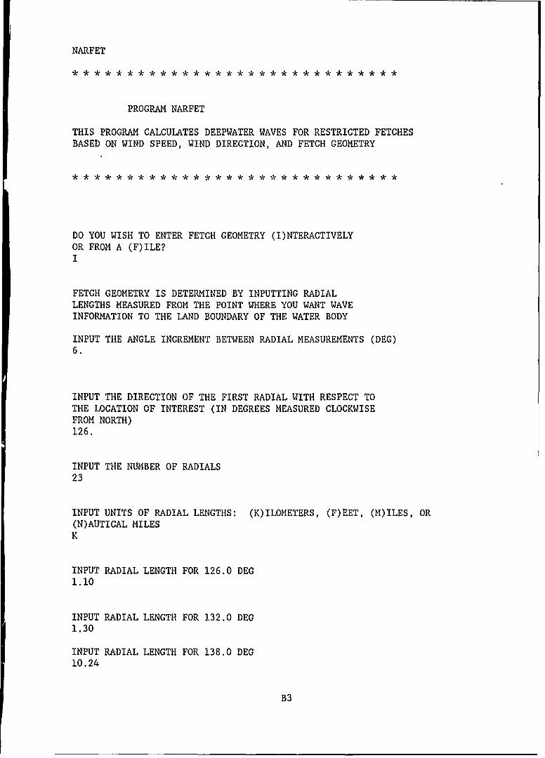
Fetch geometry

18. The first question asked by the program is "Do you wish to enter

fetch geometry interactively or from a file?" The first time the program is

run for a site, the geometry must be entered interactively. The fetch geome-

try from a run may be written to a file during the run, and that file can be

used as input for subsequent runs.

19. Fetch geometry is described by radial fetch lengths measured from

the shoreline to the point of interest at even angle increments. The next

interactive questions ask for the angle increment between input fetches, the

direction of the first fetch relative to the point of interest, and the number

of input lengths. The angle increments must be small enough to resolve the

19

shoreline, typically 5 to 10 deg. Linear interpolation is used between input

values. For many applications it is not necessary to input fetch lengths

around the full 360-deg arc, so the program allows the user to start from any

angle (angles are measured clockwise from north and represent the direction

winds/waves are coming from) and input any number of lengths (up to a 360-deg

arc). For example, for winds blowing along the long axis of the water body,

only a small arc of fetch lengths is needed. For winds blowing along the

short axis, fetch lengths along an arc of up to 180 deg may be needed. If a

complete 360-deg arc is not entered, the unspecified lengths are set to zero

and no wave generation will occur in those directions.

20. The program requests fetch lengths starting from the specified

starting direction and proceeding clockwise at the input angle increment.

Fetch lengths should be measured off a large-scale chart representing the

shoreline for the design water elevation. The units of the fetch lengths may

be kilometres, feet, miles, or nautical miles. The program converts all units

to metres for internal calculations. Figure 5 is an example of the fetch

geometry in southern Puget Sound. An angle increment of 6 deg was used.

Twenty-three fetch lengths were measured starting from an angle of 126 deg

from north. See Appendix B for this sample run. After all radial lengths are

entered, the program lists the lengths, so the user can check for errors.

Errors can be corrected by entering the number of values to be changed, then

entering the angle and new radial length for each change.

21. NARFET internally interpolates fetch lengths at 1-deg increments

around the entire 360-deg arc. Then the program averages fetch lengths over

15-deg arcs centered on each 1-deg increment. These fetch lengths are used to

calculate wave conditions. The option is given to write this information to a

file for future runs, in which case a file name is requested.

Wind forcing

22. kind forcing is represented by wind speed, direction, and duration

over the water body. Wind fields are distorted by frictional effects, so the

measurement elevation, the boundary layer stability, and the measurement loca-

tion (overland or overwater) are also needed to adjust the wind speed to

standard conditions. The simplified corrections to the wind speed used in

NARFET are based on these three factors. The correction methods are given in

the SPH. The standard elevation of wind measurements is 10 m, so in the

program wind speeds are adjusted to the 10-m elevation. The air-sea tempera-

ture difference represents the boundary layer stability. If the air-sea

20

0

t-,41

bfj

4)

.4

21

temperature difference is unknown, the SPM recommends a correction factor of

1.1 (unstable condition). This correction factor is equivalent to an air-sea

temperature difference of approximately -30 C. Overland wind conditions

differ from overwater conditions because of increases in surface roughness

overland. An additional correction is made if winds are based on overland

measurements.

23. After these three corrections to the wind speed are made, the wind

speed is converted to a wind stress factor by applying the nonconstant coeffi-

cient of drag correction (SPM). Wave growth is driven by wind stress, which

is a function of wind speed and a drag coefficient. The drag coefficient is

also a function of wind speed. This correction accounts for the change in the

drag coefficient with wind speed (making winds more effective at high wind

speeds), and it increases wave heights at high wind speeds. The nonconstant

coefficient of drag correction was not used in developing NARFET (this is an

area of present research), but current Corps of Engineers guidance recommends

using the correction. The duration input is used to check if wave generation

is limited by duration. The program does not convert very short duration wind

observations (e.g., fastest mile wind speeds) to longer durations.

Program Output

24. When all input is complete, NARFET determines the direction of wave

generation from the input wind direction by maximizing the wave period from

Equation 9. The maximum period is achieved when:

(cos ) 0 44F0 .2 8 (11)

is maximized, where F is the 15-deg averaged fetch length at an angle

with the wind direction. When the fetch and angle that maximize Equation 11

are determined, the fetch, angle, and wind speed are applied to Equation 9 to

calculate wave height and period.

25. The purpose of this study was to redefine the fetch for fetch-

limited conditions, but it is difficult to know a priori if fetch-limited

conditions exist. Therefore, the program checks for exceedence of duration-

limited and fully developed conditions. Duration-limited conditions exist if

the integral of the transit time (inverse of wave celerity) across the fetch

exceeds the wind duration. If duration is the limiting factor, the SPM

22

expression for duration-limited conditions is used. Duration-limited wave

generation in the off-wind direction is allowed. Wave conditions are also

compared with fully developed conditions (based on the expression in the SPM)

for the input wind speed. If fully developed conditions are exceeded, the SPM

expression is used to calculate wave height and period. Shallow-water wave

conditions can be estimated by applying the fetch calculated by Equation 11 to

the shallow-water wave forecasting curves in the SPM (1984).

26. The program prints the wave height (in feet and meters), period,

and direction at the end of the run. Input wind conditions (including the

wind speed adjusted for elevation, stability, and location) are also printed

for easy reference. The program states whether the solution is fetch-limited,

duration-limited, or fully developed. The option is given to calculate addi-

tional wave conditions for new wind input or terminate the run.

23

PART IV: CONCLUSIONS

27. Wave generation in off-wind directions is significant for re-

stricted fetch geometries. Models that do not consider generation in off-

wind directions underestimate wave conditions for winds blowing along the

shorter fetches of an irregularly shaped water body. Estimation of fetch

lengths over large arcs (90 to 180 deg), as in the effective fetch and

spectral contribution models, also underestimates wave conditions. The model

proposed by Donelan gives reasonable results for restricted fetches, but it

has been criticized because of the relationship between fetch and wave height.

A better expression, based on the data set compiled for this study, is given

by Equation 9. Additional data are needed to independently verify Equation 9.

The simple computer program NARFET applies Equation 9 to calculate wave

height, period, and direction given fetch geometry and wind forcing.

24

REFERENCES

Bishop, C. T. 1983. "Comparison of Manual Wave Prediction Models," Journalof Waterway. Port. Coastal and Ocean Engineering. American Society of CivilEngineers, Vol 109, No. 1, pp 1-17.

Bretschneider, C. L. 1963. "A One-Dimensional Gravity Wave Spectrum," OceanWave Spectra. Prentice-Hall, Englewood Cliffs, NJ, pp 41-56. -

Donelan, H. A. 1980. "Similarity Theory Applied to the Forecasting of WaveHeights, Periods, and Directions," Proceedings of the Canadian Coastal Confer-ence. National Research Council, Canada, pp 47-61.

Hasselmann, K., Barnett, T. P., Bouws, E., Carlson, H., Cartwright, D. E.,Enke, K., Ewing, J. A., Gienapp, H., Hasselmann, D. E., Kruseman, P.,Meerburg, A., Muller, P., Olbers, D. J., Richter, K., Sell, W., and Walden, H.1973. nMeasurements of Wind-Wave Growth and Swell Decay During the JointNorth Sea Wave Project (JONSWAP)," Deutschen Hydrographischen Zeitschrift,Supplement A, Vol 8, No. 12.

Hughes, S. A., and Jensen, R. E. 1986. "A User's Guide to SHALWV: NumericalModel for Simulation of Shallow-Water Wave Growth, Propagation, and Decay,"Instruction Report CERC-86-2, US Army Engineer Waterways Experiment Station,Vicksburg, MS.

Nelson, E. E., and Broderick, L. L. 1986. "Floating Breakwater PrototypeTest Program: Seattle Washington," Miscellaneous Paper CERC-86-3, US ArmyEngineer Waterways Experiment Station, Vicksburg, MS.

Rottier, J. R., and Vincent, C. L. 1982. "Fetch Limited Wave Growth ObservedDuring ARSLOE," Proceedings of OCEANS '82. pp 914-919.

Saville, T. 1954. "The Effect of Fetch Width on Wave Generation," TechnicalMemorandum 70, Beach Erosion Board, Washington, DC.

Seymour, R. J. 1977. "Estimating Wave Generation on Restricted Fetches,"

Journal of the Waterway, Port, Coastal and Ocean Division, American Society ofCivil Engineers, Vol 103, No. WW2, pp 251-264.

Shore Protection Manual. 1966 and 1984. US Army Engineer Waterways Experi-ment Station, Coastal Engineering Research Center, US Government PrintingOffice, Washington, DC.

US Army Corps of Engineers. 1962. "Waves in Inland Reservoirs (Summary Re-port on Civil Works Investigation Projects CW-164 and CE-165)," TechnicalMemorandum 132, Beach Erosion Board, Washington, DC.

Walsh, E. J., Hancock, D. W., III, Hines, D. E., Swift, R. N., and Scott,J. F. In Preparation. "Evolution of the Directional Wave Spectrum fromShoreline to Fully Developed," Submitted to Journal of Physical Oceanography.

25

APPENDIX A: DATA

Al

Puget Sound, Fort Peck Reservoir, Denison Reservoir, and Lake Ontario Data

U Dir Elev Temp H T X F 4 DurID (mis) (deg) (ft) cor ( (s) (km (km) (deg) (hr)

PS011083 10.76 184.3 30. 1.0 0.98 3.77 18.8 22.4 4. 6.0PS040883 6.26 215.1 30. 1.0 0.21 2.67 5.9 22.4 36. 14.0PS120883 8.45 190.3 30. 1.134 0.80 3.75 14.0 22.4 10. 6.0PS121983 8.12 341.6 30. 1.145 0.84 3.00 10.6 29.0 20. 10.0PS010384 5.21 177.3 30. 1.105 0.55 2.67 22.4 22.4 2. 6.0PS012384 6.02 199.2 30. 1.025 0.49 2.35 9.8 22.4 20. 6.0PS012584 10.40 207.5 30. 1.100 1.13 3.71 6.9 22.4 28. 4.0

F2090950 11.64 67.5 25. 1.0 0.46 2.69 10.5 11.2 6. 4.0F2091650 10.23 67.5 25. 1.0 0.51 2.60 10.5 11.2 6. 2.5F2101450 12.09 90.0 25. 1.0 0.54 2.92 10.4 11.4 10. 4.0F2081151 12.44 90.0 25. 1.0 0.78 2.90 10.4 11.4 10. 3.0F2082951 14.62 90.0 25. 1.0 0.61 3.10 10.4 11.4 10. 1.5F2101151 11.65 112.5 25. 1.0 0.60 2.77 9.7 12.2 14. 2.0F2060952 12.82 67.5 25. 1.0 0.84 3.08 10.5 11.2 6. 4.0F2061052 13.96 67.5 25. 1.0 0.88 3.27 10.5 11.2 6. 2.0F2061052 15.23 112.5 25. 1.0 0.90 3.28 9.7 12.2 14. 4.0F2061152 16.77 67.5 25. 1.0 1.00 3.35 10.5 11.2 6. 4.0F2061252 13.63 67.5 25. 1.0 0.83 3.30 10.5 11.2 6. 2.5F2061452 11.90 90.0 25. 1.0 0.52 3.12 10.4 11.4 10. 3.0F2081652 9.90 90.0 25. 1.0 0.61 2.85 10.4 11.4 10. 2.0F2082052 8.49 90.0 25. 1.0 0.46 2.55 10.4 11.4 10. 3.0F2082052 10.58 112.5 25. 1.0 0.54 2.68 9.7 12.2 14. 5.0F2082152 9.12 90.0 25. 1.0 0.47 2.58 10.4 11.4 10. 3.0

F3081951 14.30 22.5 25. 1.0 0.78 3.60 16.8 17.8 4. 2.5F3061252 13.07 22.5 25. 1.0 0.82 2.95 16.8 17.8 4. 5.5F3061252 10.16 45.0 25. 1.0 0.68 2.80 11.4 17.1 15. 3.0F3061452 11.00 22.5 25. 1.0 0.46 2.90 16.8 17.8 4. 3.0F3062752 10.01 22.5 25. 1.0 0.43 2.58 16.8 17.8 4. 10.0F3062952 10.99 22.5 25. 1.0 0.51 2.88 16.8 17.8 4. 3.5

DC110850 13.81 22.5 25. 1.0 0.40 2.43 1.9 8.1 28. 9.0DC120550 16.73 22.5 25. 1.0 0.34 2.57 1.9 8.1 28. 7.0DC032951 13.72 337.5 25. 1.0 0.39 2.56 2.0 4.6 24. 9.5DCII1551 13.52 337.5 25. 1.0 0.41 2.52 2.0 4.6 24. 4.0DC121251 13.55 337.5 25. 1.0 0.37 2.57 2.0 4.6 24. 9.5DC020952 14.05 0.0 25. 1.0 0.46 2.53 1.8 5.9 38. 3.5DC022952 17.22 337.5 25. 1.0 0.56 2.89 2.0 4.6 24. 2.5DC022952 12.35 337.5 25. 1.0 0.29 2.37 2.0 4.6 24. 2.5

DAI1551 13.29 337.5 25. 1.0 0.82 3.26 11.2 11.2 0. 4.5DAI1551 11.34 0.0 25. 1.0 0.56 2.68 2.7 11.2 22. 2.5DA111651 9.37 22.5 25. 1.0 0.40 2.66 2.3 10.0 38. 3.5DA022952 13.80 337.5 25. 1.0 1.07 3.21 11.2 11.2 0. 4.0DA022952 11.37 337.5 25. 1.0 0.77 2.83 11.2 11.2 0. 3.5

(Continued)

A3

(Continued)

U dir elev temp H T X F 4 durID A( 2 ). (deg) (ft) cor 0 () (.m -(km.) (deg) (hr)

DA031852 10.85 292.5 25. 1.0 0.49 2.20 2.6 9.5 38. 3.0DA031852 13.50 292.5 25. 1.0 0.74 2.40 2.6 9.5 38. 5.5DA041352 10.80 337.5 25. 1.0 0.46 2.61 11.2 11.2 0. 10.5DA040452 13.62 337.5 25. 1.0 0.57 3.12 11.2 11.2 0. 6.0DA040452 10.47 337.5 25. 1.0 0.52 2.86 11.2 11.2 0. 5.5DA051052 11.61 0.0 25. 1.0 0.65 3.03 2.7 11.2 22. 5.0DA051052 11.99 22.5 25. 1.0 0.61 2.92 2.3 10.0 38. 3.0DA051052 9.98 0.0 25. 1.0 0.48 2.67 2.7 11.2 22. 3.0DA112553 11.64 337.5 25. 1.0 0.70 2.79 11.2 11.2 0. 4.5

lo042215 12.59 133.0 13. 1.06 1.87 5.90 40.80 176.00 38. 11.0lo042221 9.12 121.0 13. 1.04 2.00 6.57 49.00 182.33 27. 7.01o045505 7.62 357.0 13. 1.03 0.56 3.18 15.87 37.58 35. 3.0

A4

APPENDIX B: SAMPLE RUN

Bi

NARFET

**** *** ************* *** *******

PROGRAM NARFET

THIS PROGRAM CALCULATES DEEPWATER WAVES FOR RESTRICTED FETCHESBASED ON WIND SPEED, WIND DIRECTION, AND FETCH GEOMETRY

**** *** ***** *** ** ****** *** ****

DO YOU WISH TO ENTER FETCH GEOMETRY (I)NTERACTIVELYOR FROM A (F)ILE?I

FETCH GEOMETRY IS DETERMINED BY INPUTTING RADIALLENGTHS MEASURED FROM THE POINT WHERE YOU WANT WAVEINFORMATION TO THE LAND BOUNDARY OF THE WATER BODY

INPUT THE ANGLE INCREMENT BETWEEN RADIAL MEASUREMENTS (DEG)6.

INPUT THE DIRECTION OF THE FIRST RADIAL WITH RESPECT TOTHE LOCATION OF INTEREST (IN DEGREES MEASURED CLOCKWISEFROM NORTH)126.

INPUT THE NUMBER OF RADIALS23

INPUT UNITS OF RADIAL LENGTHS: (K)ILOMETERS, (F)EET, (M)ILES, OR(N)AUTICAL MILESK

INPUT RADIAL LENGTH FOR 126.0 DEG1.10

INPUT RADIAL LENGTH FOR 132.0 DEG1.30

INPUT RADIAL LENGTH FOR 138.0 DEG10.24

B3

INPUT RADIAL LENGTH FOR 144.0 DEG9.75

INPUT RADIAL LENGTH FOR 150.0 DEG

7.88

INPUT RADIAL LENGTH FOR 156.0 DEG8.21

INPUT RADIAL LENGTH FOR 162.0 DEG8.62

INPUT RADIAL LENGTH FOR 168.0 DEG35.68

INPUT RADIAL LENGTH FOR 174.0 DEG28.24

INPUT RADIAL LENGTH FOR 180.0 DEG20.20

INPUT RADIAL LENGTH FOR 186.0 DEG16.01

INPUT RADIAL LENGTH FOR 192.0 DEG12.76

INPUT RADIAL LENGTH FOR 198.0 DEG8.21

INPUT RADIAL LENGTH FOR 204.0 DEG8.17

INPUT RADIAL LENGTH FOR 210.0 DEG7.48

INPUT RADIAL LENGTH FOR 216.0 DEG5.20

INPUT RADIAL LENG7H FOR 222.0 DEG5.08

B4

INPUT RADIAL LENGTH FOR 228.0 DEG4.47

INPUT RADIAL LENGTH FOR 234.0 DEG4.15

INPUT RADIAL LENGTH FOR 240.0 DEG4.39

INPUT RADIAL LENGTH FOR 246.0 DEG4.55

INPUT RADIAL LENGTH FOR 252.0 DEG4.63

INPUT RADIAL LENGTH FOR 258.0 DEG4.59

RECAP OF INPUT ANGLES AND RADIAL LENGTHS

ANGLE - 126.0 RADIAL LENGTH - 1.10ANGLE - 132.0 RADIAL LENGTH - 1.30ANGLE - 138.0 RADIAL LENGTH - 10.24ANGLE - 144.0 RADIAL LENGTH - 9.75ANGLE - 150.0 RADIAL LENGTH - 7.88ANGLE - 156.0 RADIAL LENGTH - 8.21ANGLE - 162.0 RADIAL LENGTH - 8.62ANGLE - 168.0 RADIAL LENGTH - 35.68ANGLE - 174.0 RADIAL LENGTH - 28.24ANGLE - 180.0 RADIAL LENGTH - 20.20ANGLE - 186.0 RADIAL LENGTH = 16.01ANGLE - 192.0 RADIAL LENGTH - 12.76ANGLE - 198.0 RADIAL LENGTH = 8.21ANGLE - 204.0 RADIAL LENGTH = 8.17ANGLE = 210.0 RADIAL LENGTH - 7.48ANGLE - 216.0 RADIAL LENGTH - 5.20ANGLE - 222.0 RADIAL LENGTH = 5.08ANGLE - 228.0 RADIAL LENGTH - 4.47ANGLE - 234.0 RADIAL LENGTH = 4.15ANGLE - 240.0 RADIAL LENGTH - 4.39ANGLE = 246.0 RADIAL LENGTH = 4.55ANGLE - 252.0 RADIAL LENGTH - 4.63ANGLE - 258.0 RADIAL LENGTH - 4.59

HOW MANY VALUES DO YOU WISH TO CHANGE?(ENTER 0 FOR NONE)0

B5

DO YOU WISH TO SAVE FETCH GEOMETRY FORFUTURE RUNS? (Y OR N)Y

ENTER FILE NAME (MAX OF 8 CHARACTERS) TOSAVE FETCH GEOMETRYPUGS.DAT

INPUT UNITS OF WIND MEASUREMENT ELEVATION: (M)ETERS OR (F)EETM

INPUT WIND MEASUREMENT ELEVATION10.

IS THE OBSERVATION LOCATION OVER WATER (W) OR LAND (L)?W

INPUT UNITS OF AIR-SEA TEMPERATURE DIFFERENCE: DEGREES (C) OR (F)C

INPUT UNITS OF WIND SPEED: (M)ETERS/SEC, (F)EET/SEC, (K)NOTS,OR MILES/HOUR (N)M

INPUT AIR - SEA TEMPERATURE DIFFERENCE-3.

INPUT WIND SPEED, WIND DIRECTION (DEC), AND DURATION (HR)15.,200.,5.

INPUT CONDITIONS:ADJUSTED WIND SPEED (M/S) - 22.7 ( 22.7 INPUT UNITS)WIND DIRECTION (DEG) - 200.0DURATION (HR) - 5.0AIR-SEA TEMP DIF (DEC C) - -3.0

WAVE HEIGHT (M) = 1.6WAVE HEIGHT (FT) = 5.3WAVE PERIOD (S) - 4.7WAVE DIRECTION (DEG) = 173.0

B6

DURATION LIMIT (HR) = 2.9

FETCH LIMITED CONDITIONS

DO YOU WANT TO RUN ANOTHER WIND CONDITION?Y

INPUT AIR - SEA TEMPERATURE DIFFERENCE0.

INPUT WIND SPEED, WIND DIRECTION (DEG), AND DURATION (HR)15.,175.,5.

INPUT CONDITIONS:ADJUSTED WIND SPEED (M/S) - 19.9 ( 19.9 INPUT UNITS)WIND DIRECTION (DEG) - 175.0DURATION (HR) - 5.0AIR-SEA TEMP DIF (DEG C) - 0.0

SIGNIFICANT WAVE HEIGHT (M) - 1.6SIGNIFICANT WAVE HEIGHT (FT) - 5.2PEAK WAVE PERIOD (S) - 4.7MEAN WAVE DIRECTION (DEG) - 172.0

DURATION LIMIT (HR) - 3.0

FETCH LIMITED CONDITIONS

DO YOU WANT TO RUN ANOTHER WIND CONDITION?N

RUN COMPLETEFORTRAN STOP

B7

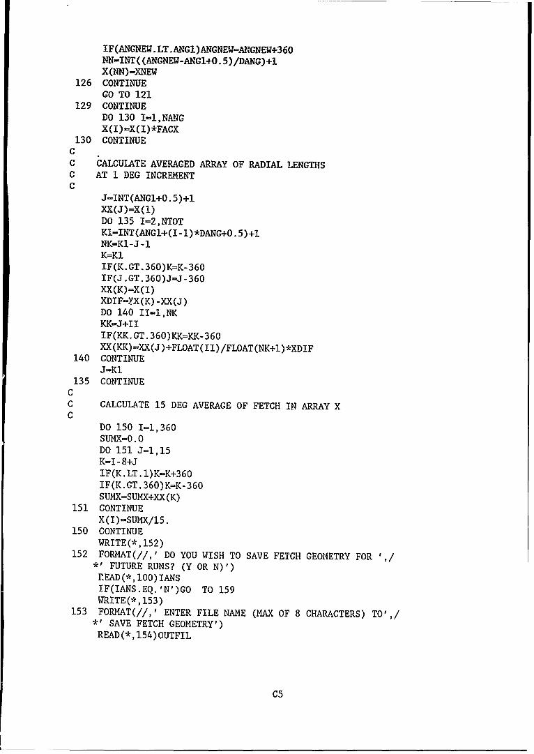
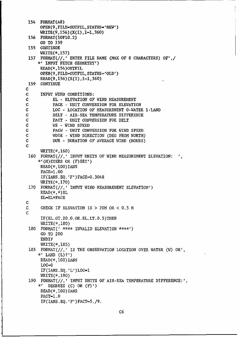
APPENDIX C: COMPUTER PROGRAM

Cl

PROGRAM NARFETC********************PROGRAM NARFET********************CC PURPOSE: TO PREDICT DEEPWATER SURFACE GRAVITYC WAVES FROM THE WIND ON RESTRICTED FETCHESCC INPUT: WS WIND SPEEDC WDIR WIND DIRECTIONC DUR DURATIONC X RADIAL FETCH DISTANCEC DANG ANGLE INCREMENT FOR FETCH MEASUREMENTSCC OUTPUT: H WAVE HEIGHTC T WAVE PERIODC THETA WAVE DIRECTIONCC

DIMENSION X(361),ANG(361),XX(361)CHARACTER*I IANSCHARACTER*8 OUTFIL

CC ZERO RADIAL LENGTH ARRAYSC X -- INPUT ARRAY AT DANG INCREMENTC XX -- AVERAGED ARRAY AT I DEG INCREMENTC

G-9.81DO 10 1-1,361X(I)=o.OXX(I)-0.O

10 CONTINUECC INTRODUCTIONC

WRITE(*,20)20 FORMAT(1X,30('* 1),//)

WRITE(*,30)30 FORMAT(11X,'PROGRAM NARFET',//,

*' THIS PROGRAM CALCULATES DEEPWATER WAVES FOR RESTRICTED FETCHES',*/,' BASED ON WIND SPEED, WIND DIRECTION, AND FETCH GEOMETRY',//)WRITE(*,20)WRITE(*,35)

35 FORMAT(//,' DO YOU WISH TO ENTER FETCH GEOMETRY (I)NTERACTIVELY',/,*' OR FROM A (F)ILE?')READ(*,100)IANSIF(IANS.EQ.'F')GO TO 155

CC START FETCH GEOMETRY INPUTC INPUT: DANG - ANGLE INCREMENTC ANGI - DIRECTION OF 1ST RADIAL INPUTC NANG - NUMBER OF INPUT RADIALSC FACX - UNITS OF RADIAL LENGTHSC

WRITE(*,40)40 FORMAT(//,' FETCH GEOMETRY IS DETERMINED BY INPUTING RADIAL',

C3

*1'LENGTHS MEASURED FROM THE POINT WHERE YOU WANT WAVE',*/'INFORMATION TO THE LAND BOUNDARY OF THE WATER BODY' ,/)

WRITE(*, 50)50 FORMAT(' INPUT THE ANGLE INCREMENT BETWEEN RADIAL MEASUREMENTS',

*'(DEG)')READ(*,*)DANGWRITE(*, 60)

60 FORMAT(//,*/'INPUT THE DIRECTION OF THE FIRST RADIAL WITH RESPECT TO',*/'THE LOCATION OF INTEREST (IN DEGREES MEASURED CLOCKWISE',*/'FROM NORTH)')

READ(* ,*)ANG1WRITE(*, 70)

70 FORMAT(//,' INPUT THE NUMBER OF RADIALS')READ(*,*)NANGWRITE(*, 80)

80 FORMAT(//,' INPUT UNITS OF RADIAL LENGTHS: (K)ILOMETERS,',*' (F)EET, (M)ILES, OR',/,' (N)AUTICAL MILES')READ(*, 100) TANSFACX=1000.IF(IANS.EQ. 'F')FACX-0.3048IF(IANS.EQ. 'M')FACX-1609.3IF(IANS.EQ. 'N')FACX=1852.0

CC READ IN ARRAY X OF RADIAL LENGTHSC

DO 110 I-1,NANGANG(l)-ANG14+(I-1)*DANGIF(ANG(I) .GE.360.)ANG(I)-ANG(I)-360.WRITE(*, 120)ANG(I)

120 FORMAT(//,' INPUT RADIAL LENGTH FOR ',F5.1,' DEG')READ(*,*)X(I)X (I)-XCI)

110 CONTINUENTOT-INT(C360/DANG)+1X (NIOT) -X (1)ANG(NTOT)-ANG (1)

CC PRINT RADIAL LENGTH FOR CHECKC121 WRITE(*,122)122 FORMT(//,1X,'RECAP OF INPUT ANGLES AND RADIAL LENGTHS',//)

DO 123 I=1,NANGWRITE(*,124)ANG(I) ,X(I)

124 FORMAT(lX,'ANGLE -',F5.1,' RADIAL LENGTH -',F9.2)123 CONTINUE

WRITE(*,125)125 FORMAT(//,1X,'HOW MANY VALUES DO YOU WISH TO CHANGE?',

*/,1X,'(ENTER 0 FOR NONE)')READ(*,*)NCHANGEIF(NCHANGE.EQ.0)GO TO 129DO 126 I-1,NCHANGEWRITE(*, 127)

127 FORIAT(X'INPUT ANGLE AND NEW RADIAL LENGTH')READ(* ,*)ANGNEW,XNEW

C4

IF(ANGNEW.-LT.ANG1)ANGNEW=AN.1 GNEW-i360NN-INT(C(ANGNEiJ-ANG1+O. 5)/DAN'G)+1X(NN)-XNEW

126 CONTINUEGO TO 121

129 CONTINUEDO 130 I=1,NANGX( I)=X(I )*FACX

130 CONTINUECC CALCULATE AVERAGED ARRAY OF RADIAL LENGTHSC AT 1 DEG INCREMENTC

J=INT(ANG1i-. 5)+1XX(J)-X(1)DO 135 I=2,NTOTK1-INT(ANG1+(I-1)*DANqG+O. 5)+1NK=K1-J-1K=KlIF(K.GT. 360)K=K-360IF(J .GT. 360)J=J-360XX(K)=X(I)XDIF=)!X(K) -XX(J)DO 140 II=1,NKKK=J+IIIF(KK.GT. 360)KK=KK-360XX(KK)=XX(J )+FLOAT(II )/FLOAT(NK 1)*xDIF

140 CONTINUEJ-K1

135 CONTINUECC CALCULATE 15 DEG AVERAGE OF FETCH IN ARRAY XC

DO 150 I=1,360SUMX=oODO 151 J=1,15K-I-8+JIF(K.LT. 1)K-K+360IF(K.GT. 360)K=K-360SUMX=SUMX+XX (K)

151 CONTINUEX(I)-SUMX/15.

150 CONTINUEWRITE(*, 152)

152 FORMAT(//,' DO YOU WISH TO SAVE FETCH GEOM4ETRY FOR'1*' FUTURE RUNS? (Y OR N)')READ(*, 100) IANSIF(IANS.EQ.'N')GO TO 159WRITE(*, 153)

153 FORMAT(//,' ENTER FILE NAME (MAX OF 8 CHARACTERS) TO',/*' SAVE FETCH GEOMETRY')READ(*, 154)OUTFIL

CS

154 FORMAT(A8)OPEN(9, FILEOUTFIL, STATUS- 'NEW')WRITE(9,156) (X(i), i=1,360)

156 FORHAT(1OF10.2)GO TO 159

155 CONTINUEWRITE(*, 157)

157 FORMAT(//,' ENTER FILE NAME (MAX OF 8 CHARACTERS) OF',/*' INPUT FETCH GEOMETRY')READ(*,154) OUTFILOPEN(9,FILE--OUTFIL, STATUS='OLD')READ(9,156)(X(I),I=1,360)

159 CONTINUECC INPUT WIND CONDITIONS:C EL - ELEVATION OF WIND MEASUREMENTC FACE - UNIT CONVERSION FOR ELEVATIONC LOC - LOCATION OF MEASUREMENT O-WATER 1-LANDC DELT - AIR-SEA TEMPERATURE DIFFERENCEC FACT - UNIT CONVERSION FOR DELTC WS - WIND SPEEDC FACW - UNIT CONVERSION FOR WIND SPEEDC WDIR - WIND DIRECTION (DEG FROM NORTH)C DUR - DURATION OF AVERAGE WIND (HOURS)C

WRITE(*, 160)160 FORMAT(//,' INPUT UNITS OF WIND MEASUREMENT ELEVATION: ',

*'(M)ETERS OR (F)EET')

READ(*, 100)IANSFACE-1.00IF(IANS.EQ. 'F')FACE=0.3048WRITE(*, 170)

170 FORMAT(//,' INPUT WIND MEASUREMENT ELEVATION')READ(*,*)ELEL=EL*FACE

CC CHECK IF ELEVATION IS > 20M OR < 0.5 MC

IF(EL.GT.20.O.OR.EL.LT.O.5)THENWRITE(*, 180)

180 FORMAT(' **** INVALID ELEVATION ****')

GO TO 200ENDIFWRITE(*, 185)

185 FORMAT(//,' IS THE OBSERVATION LOCATION OVER WATER (W) OR',*' LAND (L)?')READ(*, 100)IANSLOC-0IF(IANS.EQ. 'L')LOC=1WRITE(*, 190)

190 FORMAT(//,' INPUT UNITS OF AIR-SEA TEMPERATURE DIFFERENCE:',*' DEGREES (C) OR (F)')

READ(*,I00) IANSFACT-I. 0IF(IANS.EQ. 'F')FACT=5./9.

C6

WRITE(*, 240)240 FORMAT(//,' INPUT UNITS OF WIND SPEED: (M)ETERS/SEC,',

*' (F)EET/SEC, (K)NOTS, ',/,' OR MILES/HOUR (N)')READ(*, 100)IANSFACW-1..0IF(IANS.EQ. 'F')FACW=O.3048IF(IANS.EQ. 'K')FACW=0.51444IF(IANS.EQ. 'N')FACW=0.44704

250 CONTINUE*WRITE(*, 210)

210 FORM4AT(//' INPUT AIR - SEA TEMPERATUR.E DIFFERENCE')READ(*,*)DELTDELT=FACT*DELT

CC CHECK IF DELT IS REASONABLE -20.0< DELT < 20.0C

IF(DELT.GT.20.O.OR.DELT.LT. -20.0)THENWRITE(*, 220)

220 FORMAT(/,' **** INVALID TEMPERATURE DIFFERENCE **'

GO TO 200ENDIFWRITE(*, 260)

260 FORMAT(//,' INPUT WIND SPEED, WIND DIRECTION (DEG), AND',*' DURATION (HR)')READ(*, *)WS ,WDIR, DURWS-WS*FACW

CC CHECK IF WIND DIRECTION AND WIND SPEED ARE REASONABLEC

IF(WDIR.GT. 360.OR.WDIR.LT.O.O)THENWRITE(*, 270)

270 FORMAT(/' *** INVALID WIND DIRECTION **'

CO TO 200ENDIFIF(WS.LE.50.O)GO TO 300WRITE(*, 280)

280 FORMAT(//,' *** EXCESSIVE WIND SPEED * RESULTS INVALID')200 CONTINUE

WRITE(*, 290)290 FORMAT(/,' DO YOU WISH TO REENTER WIND CONDITIONS?')

READ(*, 100)IANSIF(IANS.EQ.'Y')GO TO 250STOP

300 DUR-DUR*3600.CC INPUT COMPLETECC ADJUST WIND SPEED FOR ELEVATION, LOCATION, AND DELTC

R=(10./EL)**(1./7.)WS-WS*RADELT=ABS (DELT)ATL=LOG(ADELT+ . 0004)/LOG(10 .0)RT=0. 932293978-O.O89853651*ATL-O.020579278*ATL*ATLIF(DELT.LT.O. 0)RT=2 . -RT

C7

WS=RT*WSIF(LOC. EQ. 1)WS=WS*(2.5*WS**(-O. 265))

CC CORRECT WIND SPEED FOR NONCONSTANT COEFFICIENT OF DRAGC

WS=0.71*WS**1.23CC DETERMINE WAVE DIRECTION FOR GIVEN WIND DIRECTIONC

PRODMAX=O.0ICENT=INT(WDIR+O. 5)+1DO 310 1-1,90K-ICENT+(I-1)KN=ICENT- (I-1)IF(KN.LT. 1)KN=KN+360IF(K.GT. 360)K=K- 360IF(X(K) .LT.X(KN))K-KNFTRY=X(K)PHITRY=FLOAT(I-1)THTRY=FLOAT(K- 1)PRODTRY-FTRY**O. 28*(COSD(PHITRY) )**O .44IF(PRODTRY. GT. PRODMAX) THENPRODMAX-~PRODTRYF=FTRYPHI-PHITRYTHETA-THTRYENDIF

310 CONTINUECC CALCULATE AND CHECK FOR DURATION LIMITC AND FULL DEVELOPMENTC

ITYPE-1THIN-Si. 09*F**(O. 72)/(G**0 28*(WS*COSD(PHI) )**O .44)IF(TMIN.LT.DUR)THEN

CC CALCULATE H AND T - NOT DURATION LIMITEDC

H-O. 0015*WS*COSD(PHI)*SQRT(F/G)FMi=2 .7*G**(O. 72)/(F**O. 28*(WS*COSD(PHI) )**O.44)T-1/FM

CC CHECK FOR FULL DEVELOPMENTC

TFULL-8 .134*(WS*COSD(PHI)/G)IF(T.GT.TFULL)CALL FULL(X,WDIR,G,DUR,PHI,THETA,T,H, ITYPE)ELSE

CC DURATION LIMITEDC

CALL DURA(X,WS.WDIR,G,DUR,PHI,THETA,T,H,ITYPE)ENDIFDUR-DUR/3 600.WSU-WS/FACWW4RITE(*,420)WS,WSU,WDIR,DUR,DELT

C8

420 FORMAT(//,1X, 'INPUT CONDITIONS:' ,/,*5X,'ADJUSTED WIND SPEED (M/S) =',F6.1,' (',F6.1,' INPUT UNITS)',/,*5X,'WIND DIRECTION (DEG) -',F6.1,/,*5X,'DURATION (HR) =',F6.1,/,*5X,'AIR-SEA TEMP DIF (DEG C) =',F6.1)HFEET-H*3. 28WRITE(*,430)H,HFEET,T,THETA

430 FORMAT(//' SIGNIFICANT WAVE HEIGHT (M)= ,51/*'SIGNIFICANT WAVE HEIGHT (FT) - ,51/*PEAK WAVE PERIOD (S) - ',F5.1,

*/,' MEAN WAVE DIRECTION (DEG) - ',F5.1)TMIN=TMIN/3 600.WRITE(*, 431)TMIN

431 FORMAT(//,1X,'DURATION LIMIT (HR) - ',F5.1)IF(ITYPE.EQ. 1)WRITE(*,435)IF(ITYPE. EQ. 2)WRITE(*,436)IF(ITYPE.EQ.3)WRITE(*,437)

435 FORMAT(/,' FETCH LIMITED CONDITIONS')436 FORMAT(/,' DURATION LIMITED CONDITIONS')437 FORMAT(/,' FULLY DEVELOPED CONDITIONS')C

WRITE(* ,440)440 FORMAT(//,' DO YOU WANT TO RUN ANOTHER WIND CONDITION?')

READ(*, 100)IANS100 FORMAT(Al)

IF(IANS.EQ.'Y')GO TO 250WRITE(* ,450)

450 FORMAT(//,' RUN COMPLETE')STOPEND

CCC

SUBROUTINE DURA(X,WS,WDIR,G,DUR,PHI,THETA,T,H,ITYPE)CC SUBROUTINE TO DETERMINE MAX T FOR DURATION LIMITEDC CONDITIONS AT OPTIMUM PHI, BUT FETCH LIMITEDC CONDITIONS AT WDIRC

DIMENSION X(361)CC DETERMINE T FOR SIMPLE FETCHC

ICENT-INT(WDIR+0. 5)+1TMAX-O.O

CC LOOP THROUGH +/- 90 DEG UNTIL REACH DURATION-LIMITEDC KEEP TRACK OF MAX FOR FETCH LIMITED (FOR DIRECTONSC NOT DURATION LIMITED) AND USE IF GREATER THANC FIRST DURATION LIMITED CONDITIONC

DO 10 I=1,90K=ICENT+(I -1)KN=ICENT- (I-i)IF(KN .LT. 1)KN-KN+360

C9

IF(K.GT.360)K=K-360PHIK-FLOAT(I-1)IF(X(K).LT.X(KN))K-KN

CC CHECK IF DIRECTION K WITH PHIK IS DURATION LIMITEDC

TMIN=47.12*X(K)**.72/(G**O.28'(WS*COSD(PHIK))**0.44)IF(TMIN.LE.DUR)GO TO 50

CC IT IS DURATION LIMITED, SO CALCULATE ASSOCIATED TC

TDUR=O.082*DUR**0.39*(WS*COSD(PHIK)/G)**0.61CC CHECK IF FULLY DEVELOPEDC

TFULL-8.134*(WS*COSD(PHIK)/G)IF(TDUR. GT.TFULL)THENT-TFULLH-O.2433*(WS*COSD(PHIK))**2/GITYPE=3ELSET-TDURH-0.000103*DUR**0.69*(WS*COSD(PHIK))**1.31/G**0.31ITYPE-2ENDIFIF(T.LE.TMAX)GO TO 20

CC T IS GREATER THAN PREVIOUS TMAX FROM FETCH LIMITEDC CONDITIONS, SO RETURNC

PHI-PHIKTHETA-FLOAT(K-i)RETURN

20 CONTINUECC DURATION LIMITED, BUT PREVIOUS TMAX FROM FETCHC LIMITED CONDITIONS IS GREATER, SO USE PREVIOUSC TMAX AND CALCULATED ASSOCIATED H AND RETURNC

T-TMAXPHI-PHIMAXTHETA-FLOAT(KMAX-1)

H-Hi AXITYPE-ITYPEMAXRETURN

50 CONTINUEC

C CONDITIONS STILL NOT DURATION LIMITEDC CHECK IF T IS GREATER THAN TMAX AND CONTINUEC

T=X(K)**O.28w(WS*COSD(PHIK))**0.44/(2.7*G**0.72)H=0.0015*WS*COSD(PHIK)*SQRT(X(K)/G)

ITYPE-1CC CHECK IF FULLY DEVELOPED

CIO

CTFULL-8. 134*(WS*COSD(PHIK)/G)IF(T. GT.TFULL)THENT-TFULLH-O 2433*(WS*COSD(PHIK) )**2/GITYPE=3ENDIFIF(T. GT.TMAX)THENTMAX-T

.HMAX=.HPHIMAX-PHIKYkM=KITYPE=ITYPEMAXENDIF

10 CONTINUEWRITE(*, 30)

30 FORMAT(//,' ERROR, DURATION LIMITED CONDITIONS NOT FOUND')STOPEND

CCC

SUBROUTINE FULL(X,WS,WDIR,G,DUR,PHI,THETA,T,H,ITYPE)CC SUBROUTINE TO DETERMINE MAX T FOR CASE OF FULLY DEVELOPEDC CONDITIONS AT OPTIMUM PHI, BUT FETCH LIMITEDC CONDITIONS AT WDIRC

DIMENSION X(361)CC DETERMINE T FOR SIMPLE FETCHC

ICENT-INT(WDIR+O 5)+1TMAX-0.0

CC LOOP THROUGH +/- 90 DEG UNTIL REACH FULLY DEVELOPEDC KEEP TRACK OF MAX FOR FETCH LIMITED (FOR DIRECTONSC NOT FULLY DEVELOPED) AND USE IF GREATER THANC FIRST FULLY DEVELOPED CONDITIONC

DO 10 1=1,90K-ICENT+(I-1)KN-ICENT- (I-i)IF(KN.LT. 1)KN=KNi360IF(K.GT. 360)K-K- 360PHIK-FLOAT (I)IF(X(K) .LT.X(KN))K-KN

CC CHECK IF DIRECTION K WITH P111K IS FULLY DEVELOPEDC

T-X(K)**0.28*(WS*COSD(PHI))**0.44/(2.7*G**0.72)TFULL-8.134*(WS*COSD(PHIK)/G)IF(TFULL. LT.T)THEN

CC IT IS FULLY DEVELOPED

Cl

CIF(TFULL. GT. TMAX)THEN

CC T IS GREATER THAN PREVIOUS TMAX FROM FETCH LIMITEDC CONDITIONS, SO CALCULATE ASSOCIATION H AND RETURNC

PHI=PHIKT-TFULLH=0. 2433*(WS*COSD(PHIK))**2/GTHETA-FLOAT(K- 1)ITYPE-3RETURNELSE

CC FULLY DEVELOPED, BUT PREVIOUS TMAX FROM FETCHC LIMITED CONDITIONS IS GREATER, SO USE PREVIOUSC TMAX AND CALCULATE ASSOCIATED H AND RETURNC

T-TMAXPHI-PHIMAXTHETA-FLOAT(KMAX- 1)H-0. 0015*WS*COSD(PHI)*SQRT(X(KMAX)/G)ITYPE-1RETURNENDIFELSE

CC CONDITIONS STILL NOT FULLY DEVELOPEDC CHECK IF T IS GREATER THAN TMAX AND CONTINUEC

IF(T. GT.TMAX)THENTMAX-TPHIMAX-PHIKKMAX-KENDIFENDIF

10 CONTINUEWRITE(*,30)

30 FORMATk//,' ERROR, FULLY DEVELOPED CONDITIONS NOT FOUND')STOPEND

CFUNCTION COSD(ANGLE)PI-4.*ATAN(1.O)COSD-COS (ANGLE*PI/180.)RETURNEND

C

C12

APPENDIX D: NOTATION

Dl

F Straight-line fetch in the direction of the waves

Feff Effective fetch

f Frequency

fp Peak frequency

_p dimensionless peak frequency

g Gravitational acceleration

H Significant wave height

H Dimensionless significant wave height

r Correlation coefficient

Si Component of energy spectrum

T Peak wave period

U Wind speed

U' U (cos q)

X Fetch

Xi Length of the straight-line fetch

R Dimensionless fetch in wave direction

y Mean of the measured valuesA

y Predicted value

y Measured value

01 Angle from mean wind direction

AO Angle increment

p Exponent in Walsh et al. expression

Angle between the wind and wave direction

D3