Winter 2002 Arthur Keller – CS 180 5–1

Schedule• Today: Jan. 17 (TH)

Relational Algebra. Read Chapter 5. Project Part 1 due.

• Jan. 22 (T) SQL Queries. Read Sections 6.1-6.2. Assignment 2 due.

• Jan. 24 (TH) Subqueries, Grouping and Aggregation. Read Sections 6.3-6.4. Project Part 2 due.

• Jan. 29 (T) Modifications, Schemas, Views. Read Sections 6.5-6.7. Assignment 3 due.

Winter 2002 Arthur Keller – CS 180 5–2

“Core” Relational AlgebraA small set of operators that allow us to manipulate

relations in limited but useful ways. The operators are:

1. Union, intersection, and difference: the usual set operators. But the relation schemas must be the same.

2. Selection: Picking certain rows from a relation.

3. Projection: Picking certain columns.

4. Products and joins: Composing relations in useful ways.

5. Renaming of relations and their attributes.

Winter 2002 Arthur Keller – CS 180 5–3

Relational Algebra

• limited expressive power (subset of possible queries)

• good optimizer possible

• rich enough language to express enough useful things

Finiteness

SELECT

π PROJECT

X CARTESIAN PRODUCT FUNDAMENTAL

U UNION BINARY

– SET-DIFFERENCE

SET-INTERSECTION

THETA-JOIN CAN BE DEFINED

NATURAL JOIN IN TERMS OF

÷ DIVISION or QUOTIENT FUNDAMENTAL OPS

UNARY

Winter 2002 Arthur Keller – CS 180 5–4

Extra Example Relations

DEPOSIT(branchName, acctNo,custName,balance)

CUSTOMER(custName,street,custCity)

BORROW(branchName,loan-no,custName,amount)

BRANCH(branchName,assets, branchCity)

CLIENT(custName,emplName)

Borrow BN L# CN AMT

T1 Midtown 123 Fred 600 T2 Midtown 234 Sally 1200 T3 Midtown 235 Sally 1500 T4 Downtown 612 Tom 2000

Winter 2002 Arthur Keller – CS 180 5–5

SelectionR1 = C(R2)

where C is a condition involving the attributes of relation R2.

ExampleRelation Sells:

JoeMenu = bar=Joe's(Sells)

bar beer priceJoe's Bud 2.50Joe's Miller 2.75Sue's Bud 2.50Sue's Coors 3.00

bar beer priceJoe's Bud 2.50Joe's Miller 2.75

Winter 2002 Arthur Keller – CS 180 5–6

SELECT () arity((R)) = arity(R)

0 card((R)) card(R)

c (R) c (R) (R)

c is selection condition: terms of form: attr op value attr op attr

op is one of < = > ≠ ≥

example of term: branch-name = ‘Midtown’

terms are connected by

branchName = ‘Midtown’ amount > 1000 (Borrow)

custName = empName (client)

Winter 2002 Arthur Keller – CS 180 5–7

ProjectionR1 = L(R2)

where L is a list of attributes from the schema of R2.

Examplebeer,price(Sells)

• Notice elimination of duplicate tuples.

beer priceBud 2.50Miller 2.75Coors 3.00

Winter 2002 Arthur Keller – CS 180 5–8

Projection (π) 0 card (π A (R)) card

(R)

arity (π A (R)) = m arity(R) =

k

π i1,...,im (R) 1 ij k distinct

produces set of m-tuples a1,...,am

such that k-tuple b1,...,bk in R where aj = bij for j = 1,...,m

π branchName, custName (Borrow)

Midtown Fred

Midtown Sally

Downtown Tom

Winter 2002 Arthur Keller – CS 180 5–9

Product

R = R1 R2

pairs each tuple t1 of R1 with each tuple t2 of R2 and puts in R a tuple t1t2.

Winter 2002 Arthur Keller – CS 180 5–10

Cartesian Product ()

arity(R) = k1 arity(R S) = k1 + k2

arity(S) = k2 card(R S) = card(R) card(S)

R S is the set all possible (k1 + k2)-tuples

whose first k1 attributes are a tuple in R

last k2 attributes are a tuple in S

R S R SA B C D D E F A B C D D' E F

Winter 2002 Arthur Keller – CS 180 5–11

Theta-JoinR = R1 C

R2

is equivalent to R = C(R1 R2).

Winter 2002 Arthur Keller – CS 180 5–12

ExampleSells = Bars =

BarInfo = Sells Sells.Bar=Bars.Name Bars

bar beer priceJoe's Bud 2.50Joe's Miller 2.75Sue's Bud 2.50Sue's Coors 3.00

name addrJoe's Maple St.Sue's River Rd.

bar beer price name addrJoe's Bud 2.50 Joe's Maple St.Joe's Miller 2.75 Joe's Maple St.Sue's Bud 2.50 Sue's River Rd.Sue's Coors 3.00 Sue's River Rd.

Winter 2002 Arthur Keller – CS 180 5–13

Theta-Join R arity(R) = r

arity(S) = s

arity (R S) = r + s

0 card(R S) card(R) card(S)

S

i j

$i $rj)R S)

R S

1 . . . r 1 . . . s

can be < > = ≠

If equal (=), then it is anEQUIJOIN

R S = (R S)c c

R(A B C) S(C D E)

result has schema T(A B C C' D E)

R.A<S.D

i j

R(ABC) S(CDE) T(ABCC’DE) 1 3 5 2 1 1 1 3 5 1 2 2 2 4 6 1 2 2 1 3 5 3 3 4 3 5 7 3 3 4 1 3 5 4 4 3 4 6 8 4 4 3 2 4 6 3 3 4 2 4 6 4 4 3 3 5 7 4 4 3

Winter 2002 Arthur Keller – CS 180 5–14

Natural JoinR = R1 R2

calls for the theta-join of R1 and R2 with the condition that all attributes of the same name be equated. Then, one column for each pair of equated attributes is projected out.

ExampleSuppose the attribute name in relation Bars was changed to bar, to match the bar name in Sells.BarInfo = Sells Bars

bar beer price addrJoe's Bud 2.50 Maple St.Joe's Miller 2.75 Maple St.Sue's Bud 2.50 River Rd.Sue's Coors 3.00 River Rd.

Winter 2002 Arthur Keller – CS 180 5–15

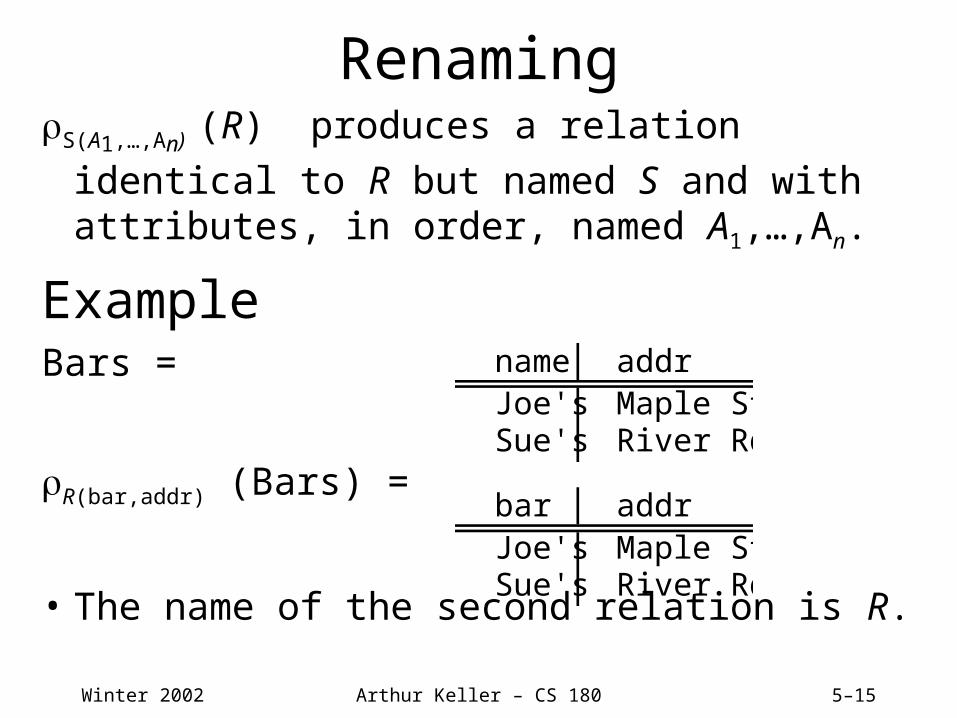
RenamingS(A1,…,An) (R) produces a relation identical to R but

named S and with attributes, in order, named A1,…,An.

ExampleBars =

R(bar,addr) (Bars) =

• The name of the second relation is R.

name addrJoe's Maple St.Sue's River Rd.

bar addrJoe's Maple St.Sue's River Rd.

Winter 2002 Arthur Keller – CS 180 5–16

Union (R S) arity(R) = arity(S) = arity(R S)

max(card(R),card(S)) card(R S)card(R) + card(S)

set of tuples in R or S or both R R S

S R S

Find customers of Perryridge Branch

πCust-Name ( Branch-Name = "Perryridge" (BORROW DEPOSIT) )

Winter 2002 Arthur Keller – CS 180 5–17

Difference(R S)

arity(R) = arity(S) = arity(R–S)

0 card(R –S)card(R) R – S R

is the tuples in R not in S

Depositors of Perryridge who aren't borrowers of Perryridge

πcustName ( branchName = ‘Perryridge’ (DEPOSIT – BORROW) )

Deposit < Perryridge, 36, Pat, 500 >

Borrow < Perryridge, 72, Pat, 10000 >

πcustName ( branchName = ‘Perryridge’ (DEPOSIT) ) —

πcustName ( branchName = ‘Perryridge’ (BORROW) )

Does (π (D) π (B) ) work?

Winter 2002 Arthur Keller – CS 180 5–18

Combining Operations

Algebra =1. Basis arguments +2. Ways of constructing expressions.For relational algebra:1. Arguments = variables standing for

relations + finite, constant relations.2. Expressions constructed by applying one

of the operators + parentheses.• Query = expression of relational algebra.

Winter 2002 Arthur Keller – CS 180 5–19

πcustName,custCity

(Client.Banker-Name = ‘Johnson’

(Client Customer) ) =

π cust-Name,custCity (Customer)

• Is this always true? Is this what we wanted?

πClient.custName, Customer.custCity

(Client.bankerName = ‘Johnson’

Client.custName = Customer.custName

(Client Customer) )

πClient.custName, CustomercustCity

(Client.custName = Customer.custName

(Customer πcustName

Client.bankerName=‘Johnson’ (Client) ) ) )

Winter 2002 Arthur Keller – CS 180 5–20

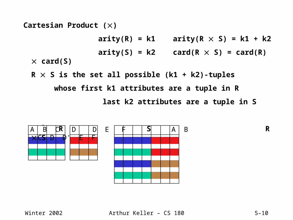
SET INTERSECTION arity(R) = arity(S) = arity (R S)

(R S) 0 card (R S) min (card(R), card(S))

tuples both in R and in S

R (R S) = R S

SR

R S R

R S S

Winter 2002 Arthur Keller – CS 180 5–21

Operator Precedence

The normal way to group operators is:

1. Unary operators , , and have highest precedence.

2. Next highest are the “multiplicative” operators, , C , and .

3. Lowest are the “additive” operators, , , and —.

• But there is no universal agreement, so we always put parentheses around the argument of a unary operator, and it is a good idea to group all binary operators with parentheses enclosing their arguments.

ExampleGroup R S T as R ((S ) T ).

Winter 2002 Arthur Keller – CS 180 5–22

Each Expression Needs a Schema• If , , — applied, schemas are the same, so use this

schema.• Projection: use the attributes listed in the projection.• Selection: no change in schema.• Product R S: use attributes of R and S.

But if they share an attribute A, prefix it with the relation name, as R.A, S.A.

• Theta-join: same as product.• Natural join: use attributes from each relation;

common attributes are merged anyway.• Renaming: whatever it says.

Winter 2002 Arthur Keller – CS 180 5–23

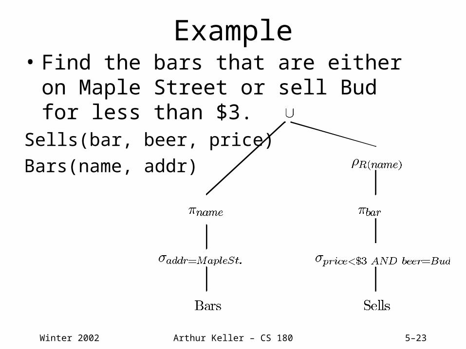
Example• Find the bars that are either on Maple Street

or sell Bud for less than $3.Sells(bar, beer, price)

Bars(name, addr)

Winter 2002 Arthur Keller – CS 180 5–24

ExampleFind the bars that sell two different beers at the

same price.

Sells(bar, beer, price)

Winter 2002 Arthur Keller – CS 180 5–25

Linear Notation for Expressions• Invent new names for intermediate relations, and assign

them values that are algebraic expressions.• Renaming of attributes implicit in schema of new relation.

ExampleFind the bars that are either on Maple Street or sell Bud for

less than $3.Sells(bar, beer, price)

Bars(name, addr)

R1(name) := name( addr = Maple St.(Bars))

R2(name) := bar( beer=Bud AND price<$3(Sells))

R3(name) := R1 R2

Winter 2002 Arthur Keller – CS 180 5–26

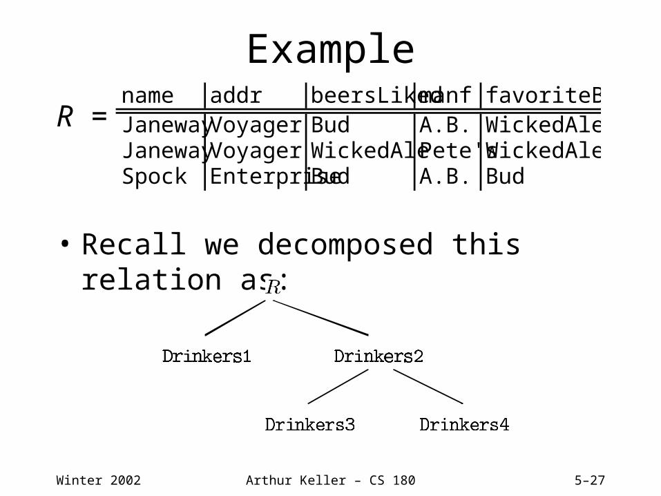
Why Decomposition “Works”?

What does it mean to “work”? Why can’t we just tear sets of attributes apart as we like?

• Answer: the decomposed relations need to represent the same information as the original. We must be able to reconstruct the original from the

decomposed relations.

Projection and Join Connect the Original and Decomposed Relations

• Suppose R is decomposed into S and T. We project R onto S and onto T.

Winter 2002 Arthur Keller – CS 180 5–27

Example

R =

• Recall we decomposed this relation as:

name addr beersLiked manf favoriteBeerJaneway Voyager Bud A.B. WickedAleJaneway Voyager WickedAle Pete's WickedAleSpock Enterprise Bud A.B. Bud

Winter 2002 Arthur Keller – CS 180 5–28

Project onto Drinkers1(name, addr, favoriteBeer):

Project onto Drinkers3(beersLiked, manf):

Project onto Drinkers4(name, beersLiked):

beersLiked manfBud A.B.WickedAle Pete'sBud A.B.

name addr beersLikedJaneway Voyager BudJaneway Voyager WickedAleSpock Enterprise Bud

name addr favoriteBeerJaneway Voyager WickedAleSpock Enterprise Bud

Winter 2002 Arthur Keller – CS 180 5–29

Reconstruction of OriginalCan we figure out the original relation from the

decomposed relations?

• Sometimes, if we natural join the relations.

ExampleDrinkers3 Drinkers4 =

• Join of above with Drinkers1 = original R.

name beersLiked manfJaneway Bud A.B.Janeway WickedAle Pete'sSpock Bud A.B.

Winter 2002 Arthur Keller – CS 180 5–30

TheoremSuppose we decompose a relation with schema XYZ into XY

and XZ and project the relation for XYZ onto XY and XZ. Then XY XZ is guaranteed to reconstruct XYZ if and only if X Y (or equivalently, X Z).

• Usually, the MVD is really a FD, X Y or X Z.

• BCNF: When we decompose XYZ into XY and XZ, it is because there is a FD X Y or X Z that violates BCNF. Thus, we can always reconstruct XYZ from its projections onto XY

and XZ.

• 4NF: when we decompose XYZ into XY and XZ, it is because there is an MVD X Y or X Z that violates 4NF. Again, we can reconstruct XYZ from its projections onto XY and XZ.

Winter 2002 Arthur Keller – CS 180 5–31

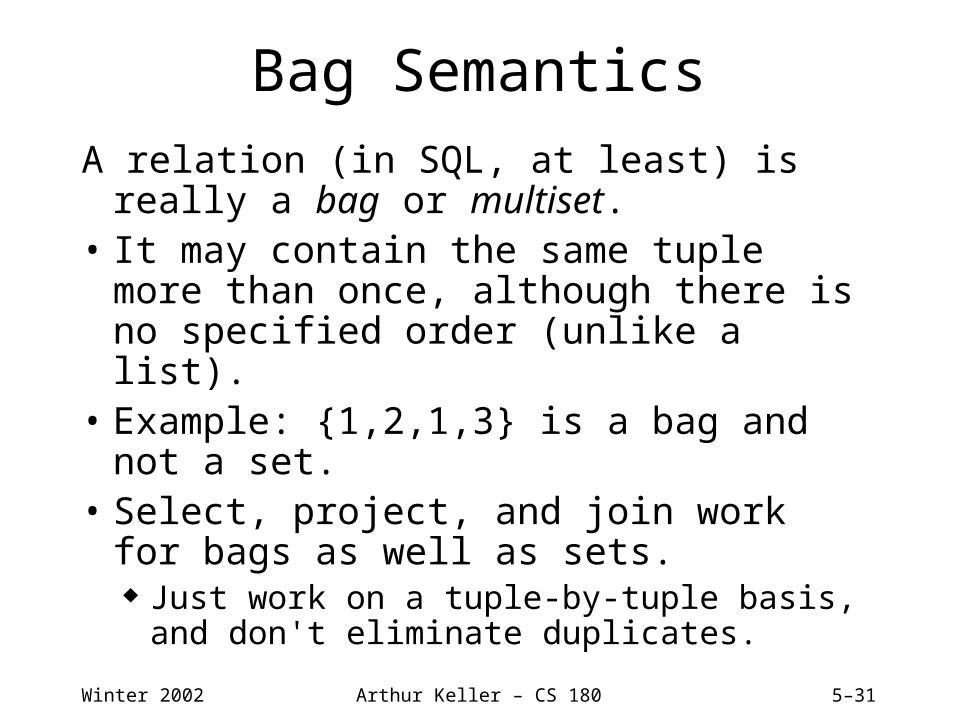
Bag Semantics

A relation (in SQL, at least) is really a bag or multiset.

• It may contain the same tuple more than once, although there is no specified order (unlike a list).

• Example: {1,2,1,3} is a bag and not a set.• Select, project, and join work for bags as

well as sets. Just work on a tuple-by-tuple basis, and don't

eliminate duplicates.

Winter 2002 Arthur Keller – CS 180 5–32

Bag Union

Sum the times an element appears in the two bags.• Example: {1,2,1} {1,2,3,3} = {1,1,1,2,2,3,3}.

Bag IntersectionTake the minimum of the number of occurrences in each

bag.• Example: {1,2,1} {1,2,3,3} = {1,2}.

Bag DifferenceProper-subtract the number of occurrences in the two bags.• Example: {1,2,1} – {1,2,3,3} = {1}.

Winter 2002 Arthur Keller – CS 180 5–33

Laws for Bags Differ From Laws for Sets

• Some familiar laws continue to hold for bags. Examples: union and intersection are still commutative and

associative.

• But other laws that hold for sets do not hold for bags.

ExampleR (S T) (R S) (R T) holds for sets.• Let R, S, and T each be the bag {1}.• Left side: S T = {1,1}; R (S T) = {1}.• Right side: R S = R T = {1};

(R S) (R T) = {1} {1} = {1,1} {1}.

Winter 2002 Arthur Keller – CS 180 5–34

Extended (“Nonclassical”)Relational Algebra

Adds features needed for SQL, bags.

1. Duplicate-elimination operator .

2. Extended projection.

3. Sorting operator .4. Grouping-and-aggregation operator .

5. Outerjoin operator o .

Winter 2002 Arthur Keller – CS 180 5–35

Duplicate Elimination(R) = relation with one copy of each tuple that appears one

or more times in R.

ExampleR =

A B1 23 41 2

(R) =A B1 23 4

Winter 2002 Arthur Keller – CS 180 5–36

Sorting L(R) = list of tuples of R, ordered according to

attributes on list L.• Note that result type is outside the normal types

(set or bag) for relational algebra. Consequence: cannot be followed by other relational

operators.

ExampleR = A B

1 33 45 2

B(R) = [(5,2), (1,3), (3,4)].

Winter 2002 Arthur Keller – CS 180 5–37

Extended Projection

Allow the columns in the projection to be functions of one or more columns in the argument relation.

ExampleR = A B

1 23 4

A+B,A,A(R) =A+B A1 A23 1 17 3 3

Winter 2002 Arthur Keller – CS 180 5–38

Aggregation Operators

• These are not relational operators; rather they summarize a column in some way.

• Five standard operators: Sum, Average, Count, Min, and Max.

Winter 2002 Arthur Keller – CS 180 5–39

Grouping Operator

L(R), where L is a list of elements that are either

a) Individual (grouping) attributes orb) Of the form (A), where is an aggregation operator

and A the attribute to which it is applied,is computed by:1. Group R according to all the grouping attributes on list L.2. Within each group, compute (A), for each element (A)

on list L.3. Result is the relation whose columns consist of one tuple

for each group. The components of that tuple are the values associated with each element of L for that group.

Winter 2002 Arthur Keller – CS 180 5–40

ExampleLet R =

bar beer priceJoe's Bud 2.00Joe's Miller 2.75Sue's Bud 2.50Sue's Coors 3.00Mel's Miller 3.25

Compute beer,AVG(price)(R).

1. Group by the grouping attribute(s), beer in this case:bar beer priceJoe's Bud 2.00Sue's Bud 2.50Joe's Miller 2.75Mel's Miller 3.25Sue's Coors 3.00

Winter 2002 Arthur Keller – CS 180 5–41

2.Compute average of price within groups:

beer AVG(price)

Bud 2.25

Miller 3.00

Coors 3.00

Winter 2002 Arthur Keller – CS 180 5–42

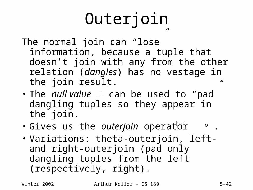
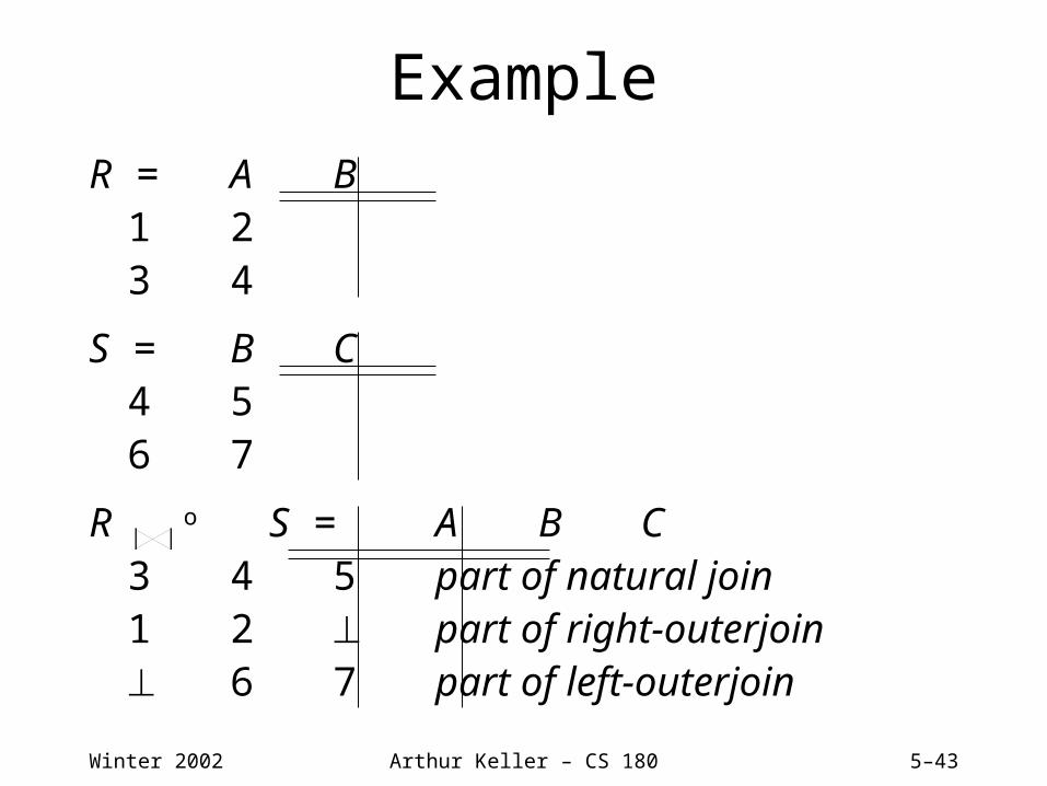
Outerjoin

The normal join can “lose” information, because a tuple that doesn’t join with any from the other relation (dangles) has no vestage in the join result.

• The null value can be used to “pad” dangling tuples so they appear in the join.

• Gives us the outerjoin operator o .• Variations: theta-outerjoin, left- and right-

outerjoin (pad only dangling tuples from the left (respectively, right).

Winter 2002 Arthur Keller – CS 180 5–43

Example

R = A B1 23 4

S = B C4 56 7

R o S = A B C3 4 5 part of natural join1 2 part of right-

outerjoin 6 7 part of left-outerjoin