Within-Year Retention Among Ph.D. Students: The Effect of Debt, Assistantships, and Fellowships Pilar Mendoza • Pedro Villarreal III • Alee Gunderson Received: 21 March 2013 Ó Springer Science+Business Media New York 2014 Abstract This study employs the 2007–2008 National Postsecondary Student Aid Study and the National Research Center’s survey data, ‘‘A Data-Based Assessment of Research-Doctorate Programs in the United States,’’ to investigate the (1) the effects of debt in relation to tuition and fees paid and (2) the effects of teaching assistantships, research assistantships, and fellowships on within year retention among Ph.D. students. We created an innovative conceptual model for this study by merging a socioeconomic model for graduate students and a graduate student socialization model. We used propensity score weights for estimating average treatment effects and average treatment effect on the treated as well as a series of control and balancing variables. This study provides timely insights into which of these financial strategies are likely to improve the already low doctoral retention rates nationwide. To the best of our knowledge, this is the first study that includes proxies of socialization variables in examining the role of various funding mechanisms in doctoral retention using a national representative dataset. Keywords Doctoral student retention Doctoral assistantships Fellowships Graduate debt Graduate students P. Mendoza (&) Deparment of Educational Leadership & Policy Analysis, College of Education, University of Missouri Columbia, 202 Hill Hall, Columbia, MO 65211, USA e-mail: [email protected]P. Villarreal III College of Education, University of Florida, Gainesville, FL, USA e-mail: [email protected]fl.edu A. Gunderson Youth Development and Agricultural Education, Purdue University, West Lafayette, IN, USA e-mail: [email protected]123 Res High Educ DOI 10.1007/s11162-014-9327-x
Transcript
Within-Year Retention Among Ph.D. Students: TheEffect of Debt, Assistantships, and Fellowships
Pilar Mendoza • Pedro Villarreal III • Alee Gunderson
Received: 21 March 2013� Springer Science+Business Media New York 2014
Abstract This study employs the 2007–2008 National Postsecondary Student Aid
Study and the National Research Center’s survey data, ‘‘A Data-Based Assessment of
Research-Doctorate Programs in the United States,’’ to investigate the (1) the effects of
debt in relation to tuition and fees paid and (2) the effects of teaching assistantships,
research assistantships, and fellowships on within year retention among Ph.D. students.
We created an innovative conceptual model for this study by merging a socioeconomic
model for graduate students and a graduate student socialization model. We used
propensity score weights for estimating average treatment effects and average treatment
effect on the treated as well as a series of control and balancing variables. This study
provides timely insights into which of these financial strategies are likely to improve
the already low doctoral retention rates nationwide. To the best of our knowledge, this
is the first study that includes proxies of socialization variables in examining the role of
various funding mechanisms in doctoral retention using a national representative
P. Mendoza (&)Deparment of Educational Leadership & Policy Analysis, College of Education, University of MissouriColumbia, 202 Hill Hall, Columbia, MO 65211, USAe-mail: [email protected]
P. Villarreal IIICollege of Education, University of Florida, Gainesville, FL, USAe-mail: [email protected]
A. GundersonYouth Development and Agricultural Education, Purdue University, West Lafayette, IN, USAe-mail: [email protected]
123
Res High EducDOI 10.1007/s11162-014-9327-x
Introduction
Graduate education produces the world’s scholars, educators, innovators, and leaders
(Walker et al. 2008). Moreover, graduate and professional degrees are increasingly being
considered the entry-level credential in many professions. In fact, it is projected that about
2.5 million jobs will require either a master’s, doctoral, or professional degree between
2008 and 2018 in the United States (Wendler et al. 2010). However, about 40 % of all
students pursuing a doctorate degree do not finish their programs (Gardner 2009). Lack of
adequate financial resources can discourage students from continuous enrollment thereby
lengthening time to degree and ultimately decreasing the probability of completion (Bowen
and Rudenstine 1992; Kim and Otts 2010; Lovitts 2001; St. John and Andrieu 1995).
In a meta-analysis, Gururaj et al. (2010) found that every form of aid is significant in
promoting graduate student retention, especially aid in the form of grants. Additionally,
financial aid in the form of assistantships that allow students’ involvement through aca-
demic tasks with their advisors and peers have been shown to be critical in graduate
retention (Gardner and Barnes 2007; Kim and Otts 2010). This indicates that in the case of
graduate education, the socialization aspect of assistantships as a form of financial aid has
important implications to retention. Nettles and Millett (2006) found that 44 % of the
doctoral students surveyed in their study were offered research assistantships, 60 %,
teaching assistantships, and 48 % fellowships. Fellowships are considered the ‘‘top prize
because they often cover all student expenses and ordinarily come with no work
requirements. Research and teaching assistantships, however, which often require students
to work with faculty on research projects or instructional activities, can be most valuable
for their associations and the apprenticeships they provide to students in preparation for
professional careers’’ (Nettles and Millett 2006, p. 74). However, time intensive forms of
financial support, such as some teaching assistantships, may impede the degree progress of
doctoral students whereas research assistantships, which align with students’ dissertation
topics, may shorten their time to degree (Kim and Otts 2010).
Nonetheless, financial aid in the form of fellowships and assistantships has not kept pace
with the rising costs of attendance, and so student borrowing has increased, although, these
trends of borrowing vary significantly by field of study and race/ethnicity (Kim and Otts
2010; Hoffer et al. 2006). The Consumer Financial Protection Bureau reported that the
outstanding student loan debt is over $1 trillion, which surpasses the amount owned on all
credit cards in the United States. In 2010–2011, federal loans accounted for 69 % of all aid
given to graduate students, who received $16,423 on average in federal loans (College
Board 2011).
Problem Statement
Assistantships, fellowships, and loans are the main financial means for doctoral students.
While student advocacy groups have become increasingly vocal against loans and the costs
of higher education continue to rise, little academic inquiry has occurred to understand
how the changing mix of these financial resources is influencing doctoral students’ decision
to enroll from fall to spring in graduate school. Previous studies suggest that various forms
of aid have differential effects on doctoral retention; however, none of these studies have
been conducted with a national representative database and with special attention to the
socialization effects of research and teaching assistantships. Therefore, in this study we
integrate findings from previous qualitative work on doctoral socialization through
Res High Educ
123
assistantships and fellowships in relation to retention with quantitative studies on graduate
student debt to investigate the effect of debt, research assistantships, teaching assistantships
and fellowships on within year doctoral retention. We used within year retention given that
the dataset available is cross-sectional and collected data on students enrolled in the
academic year 2007–2008 only.
Research Questions
• What are the effects of debt on within year retention among Ph.D. students?
• What are the effects of teaching assistantships, research assistantships, and fellowships
on within year retention among Ph.D. students?
Dataset, Sample, and Population
The main sources of data employed include the 2007–2008 National Postsecondary Student
Aid Study (NPSAS: 08) and the National Research Center’s survey data (NRC: 06), ‘‘A
Data-Based Assessment of Research-Doctorate Programs in the United States.’’ NPSAS:08
is a nationally representative dataset with postsecondary student level characteristics related
to financial aid, demographics, and academic characteristics meant to address how students
enrolled in 2007–2008 and their families pay for postsecondary education. The NRC data is
based on a departmental level survey conducted in 2005–2006 and ranks departments by
field of study based on measures of research productivity, student outcomes, and diversity. It
contains information at the doctoral departmental level related to the graduate student
experiences as well as the overall productivity, culture, and climate of individual depart-
ments. We merged these two datasets using CIP and IPEDS codes, which allowed us to
obtain variables related to the departmental characteristics for each student that are likely to
impact their graduate experiences. Although the surveys were conducted 2 years apart, we
believe that the departmental variables from NRC are likely to remain the same or minimal
changed with little impact for the purpose of this study because change in higher education
tends to be slow (Braskman and Wergin 1998; Tierney 1992).
After merging these datasets, the population of inference for these analyses became
Ph.D. students enrolled the fall of 2007 in departments ranked by the NRC survey data in
the humanities, social/behavioral sciences, life sciences, math, engineering, computer
science, health sciences and other majors throughout the nation. The sample frame is the
same used in the data collection procedure of NPSAS: 08 (Cominole et al. 2010). Sub-
sequent to matching the datasets, the sample size was (n = 1,198).
Dependent Variable
Based on the definition established by St. John and Andrieu (1995), students who were
positively retained were defined as those who were enrolled in September 2007 and in
February 2008 at the same institution. A significant percentage of students, 90 % of cases,
indicate experiencing within year retention in this data. While some researchers may
question the ability of these analyses to detect an effect due to the limited variability in the
retention outcome, we concluded, consistent with previous research, that 10 % variability
Res High Educ
123
would be sufficient to produce results that generate consistent and precise estimates given
the standard 10 events per variable guideline recommended in the statistical research
literature (Peduzzi et al. 1996).
Treatment Variables of Policy Interest
First, we defined a relative measure of debt as the ratio between cumulative graduate and
undergraduate debt over tuition and fees paid during 2007–2008 (debt-to-price ratio). This
relative measure is a better indication of students’ financial need and willingness to borrow
than using the debt amount alone; it also controls for the price differences across insti-
tutions and fields of study. However, the distribution of this variable was substantially
irregular with a significant proportion (59.4 %) of cases without a positive debt-to-price
ratio. The zero-inflated, Poisson-like distribution of this variable indicated that use of this
variable as a continuous variable in the equation would violate standard assumptions in
future analyses. Consequently, we constructed a dichotomous variable that distinguished
between subjects who indicated no debt relative to costs (entered as 0) and those subjects
who had some debt relative to costs (entered as 1).
In relation to the second research question, we measured the impact of assistantships
and fellowships on the outcome variable through three dummy variables indicating whe-
ther students received primarily a research assistantship, teaching assistantship, or fel-
lowship. After conducting a series of crosstabs, we found that 8.1 % of students in the
dataset have a research and teaching assistantships, 9.0 % a research assistantship and a
fellowship, 9.9 % a teaching assistantship and a fellowship, and 2.2 % have the three of
them. Thus, as explained below, we applied robustness checks by analyzing the models
with and without these cases with multiple assistantships/fellowships. In addition, we
controlled for the dollar amount associated with these assistantships and fellowships as an
indicator of the prevalence of each of these among students with combinations of assis-
tantships and fellowships.
While these crosstabs may indicate that the treatments are not entirely isolated from
each other, the vast majority of subjects will experience only one of these treatments
during the doctoral experiences. To reduce the number of potential outcomes into a
manageable set of dependent variables, we collapsed students with two or all three types of
fellowships and assistantships into three constructs. The operationalization of the outcome
variables resulted in the following three categorical variables: primarily teaching assis-
tantships (25.5 %), primarily research assistantships (36.9 %), and primarily Fellowships
(14.1 %) which were used as dependent variables in the Propensity Score Models and as
independent variables in the main outcome models. We were interested in understanding
the effects of teaching assistantships without the potential influence of the research
assistantship experience. Consequently, those students who reported having both teaching
and research assistantships were listed as primarily research assistantships. This opera-
tionalization will allow the effect of teaching assistantships to be exposed without the
potential confounding that could be attributed to having a research assistantship. For those
Ph.D. fellows who reported having also either or both a teaching and/or research assis-
tantship, we considered several alternatives. Because students who have a fellowship are
likely to have no specific work or other institutional obligations, we wanted to understand
these fellows without the mixed effects that could potentially influence these Ph.D. stu-
dents’ outcomes due to an assistantship. As a result, those students reporting both fel-
lowships and teaching assistantships were combined with those students who reported
Res High Educ
123
primarily teaching assistantships. Likewise, students reporting both fellowships and
research assistantships were combined with the category of students reporting primarily
research assistantships. We decided to combine students who reported both research as-
sistantships and teaching assistantships with the category of primarily research assistant-
ships because we did not want the socialization characteristics particular to the research
assistantships affecting the effects of the models of teaching assistantships. Finally, sub-
jects who reported all three were collapsed into the primarily research assistantship cat-
egory. While this recoding created a substantially greater number of subjects in the
research assistantship group, we reasoned that this operationalization was likely to have a
less deleterious effect on either outcome as explained above.
Finally, almost a quarter (23.5 %) of Ph.D. students in the sample reported not having
an assistantship or fellowship. In most analyses, this group served as the reference category
for interpretation of the treatment effects on retention. While this may seem as an
unusually small proportion of students, the sample is delimited to a select number of
doctoral universities that are nationally ranked by the National Research Council (NRC),
and the sample was also delimited to only those doctoral program areas for which the NRC
compiles a ranking. Given these delimitations, we are confident that this operationalization
of each of the outcome variables would provide the most informative and reliable con-
clusions regarding our research questions of interest.
Covariates Used as Balancing and Control Variables
The covariates included in the models were selected according to each of the six constructs in
the theoretical model developed for this study and the availability of data. We created an
innovative conceptual model for this study by merging the retention model for graduate
students as defined by St. John and Andrieu (1995) and the graduate student socialization
model created by Weidman et al. (2001). By augmenting the socioeconomic framework of
St. John and Andrieu (1995) with the socialization framework created by Weidman et al.
(2001), we were able to include a more detailed account of the factors associated with
doctoral within-year retention, especially in relation to the experience in graduate school,
which has been proven to be a critical factor in doctoral attrition in qualitative work (Gardner
2009; Golde 2000, 2005; Lovitts 2001) and correspond to one of the six constructs of St. John
and Andrieu’s model. In particular, St. John and Andrieu (1995) argue that within year
retention decisions among graduate students are a function of the following six constructs.
Social and Economic Background
A series of studies have demonstrated that the background characteristics of students such
as age, gender, race/ethnicity, SES, marital, dependent, and immigration status impact their
graduate experience and retention (Gardner and Mendoza 2010). As such, the variables
used in this construct account for the individual SES, demographics as well as immigration
and dependency status of students.
Aspirations
The highest degree expected by students influence their level of commitment to the goal of
obtaining a degree (Burton and Ramist 2001; Kim 2007). However, given that all students
in the dataset are pursuing the highest level of educational attainment, we assume that all
Res High Educ
123
students have the same aspiration, to obtain their Ph.D. Therefore there is no need to
control for this construct.
Expected Earnings Upon Graduation
This construct is based on human capital theory and relates to the labor market conditions
upon graduation that influence the cost-benefit analysis to stay enrolled (DesJardins and
McCall 2010). We obtained data from 2009 Survey of Earned Doctorates to create a
variable with the average basic annual salary for doctorate recipients for employment in the
US by field of study.
Prices
A large body of research confirms the impact of prices and subsidies in educational
attainment at all levels (Hossler et al. 2009; Kim and Otts 2010; Nettles and Millett 2006).
We controlled for the cost of attendance using two measures, the tuition and fees amount
paid and other costs besides tuition and fees paid. We used these two variables in the
models addressing the second research questions, but only other costs in the model
addressing the first question, given that the treatment variable in that case already accounts
for tuition and fees.
Price Subsidies
This construct refers to any type of discount students receive in the forms of financial aid
(grants, loans, fellowships, work-study, and waivers) and assistantships. We used two
variables to control for these subsidies, loan-based amount and non-loan based amount,
given that the first one needs to be repaid after graduation. The amount of non-loan based
subsidies was included in all analyses. Graduate loans was not included in the analysis
addressing the first research question given that the associated variable of interest already
deals with the issue of loan debt.
Graduate Experiences
The socialization of doctoral students is determined by the particular circumstances of the
student related to their socialization experiences, institutional climate and culture, disci-
plinary norms, and role of the advisor (Gardner 2009; Lovitts 2001). Likewise, the model
by Weidman et al. (2001) emphasizes the graduate experience in student socialization and
retention. Researchers have asserted that the graduate student experience occurs mainly at
the departmental level (Gardner and Mendoza 2010; Golde 2005; Tinto 1993; Weidman
et al. 2001). These graduate experiences become a series of socialization processes by
which students learn the robes of the profession and become members of a community of
scholars/practice for the rest of their careers upon graduation. In this context, doctoral
retention partially depends on the socialization processes associated with the normative
and structural character of the field of study manifested at the departmental level. Given
that socialization processes are compounded by the specific characteristics of students’
universities and departments, we used variables that as a whole relate the culture, climate,
and interactions of the students’ surroundings. However, a limitation of this study is the
lack of variables that directly measures socialization. At the very least we were able to use
Res High Educ
123
proxies of socialization related to the departmental climate of each student in the dataset.
We believe that merging two datasets to add departmental climate is an important and new
contribution of this study. These departmental characteristics are the ones included in the
NRC ranking of doctoral departments and include size and three dimensions measured by a
number of variables in each category: research activity, students support and outcomes,
and diversity. We also used several variables indicative of the particular experience of each
student such as years in the program, enrollment patterns, distance education, employment
while enrolled, and field of study.
For the main models, we used the dimensional variables constructed from a variety of
measures in order to minimize the number of variables to include in the main models.
However, for calculating the propensity score weights we used the variables listed as
variables used in ‘‘PS Model’’ or ‘‘All’’ provided in Table 1. Years in the program,
enrollment patterns, distance education, employment while enrolled, and field of study
influence how students engage and integrate into their academic, professional and personal
communities. For example, years in the program shape the experiences of doctoral students
before and after the qualifier examination (Tinto 1993). Whether students attend part time
or take distance education courses signals different ways of involvement. Disciplinary
cultures are a major source of socialization for doctoral students, and so, field of study is an
influential factor in doctoral retention (Mendoza 2007). The relationship with advisor has
been documented as a critical aspect of the doctoral experience, socialization, and attrition
(Lovitts 2001). Unfortunately, we do not have data that could account for this construct,
which constitutes a limitation of the study.
According to Malcolm and Dowd (2012) and others there are many factors, both
observable and unobservable, that contribute to a student’s decision to finance their edu-
cation through loans. In addition, a student’s decision to take out a loan for education is not
a random phenomenon; essentially, students self-select themselves into loan programs.
Similarly, according to Nettles and Millett (2006), graduate student finances are complex
involving both tangibles, such as tuition, lost wages, personal income, type of assistant-
ships, and intangibles, such as attitudes toward debt and other psychological approaches to
acquiring and using money. Additionally, selection bias to the different types of assis-
tantships is likely driven by departmental and disciplinary characteristics as well as the
educational background and predispositions of the individual student. To damper self-
selection bias on observables, we employed counterfactual methodologies as explained in
the next section.
Analysis
Stage 1: Data Augmentation, Cleaning, and Transformations
Various data conditioning and transformations were performed on the variables during this
stage to generate more normally distributed data in some variables and to test curvilinear or
nonlinear relationships in other variables. We transformed the age of subjects variable by
taking the inverse function to create a more normally distributed variable of age. Due to
considerations of time and the dimensionality of age as a construct that parallels time, we
also generated squared and cubic forms of the inverse of age to test the likely nonlinear
functional relationships between age and the various response variables included in the
models and equations. We tested various transformations of AGI and found that the square
root of AGI is most normally distributed and would perform best in latter stages of
Res High Educ
123
Table 1 List of variables, data source, and models
Outcome variable Independent variables Source Model
Within year retention:2007–2008
Variables of interest
Cumulative debt/tuition and fees NPSAS Model 1
Primarily research assistantship NPSAS Model 2
Primarily teaching assistantship NPSAS Model 3
Primarily fellowship NPSAS Model 4
Construct Covariates
Social and economicbackground
Gender NPSAS All
Race/Ethnicity NPSAS All
Age NPSAS All
Dependent and civil status NPSAS All
Family size NPSAS All
Disability status NPSAS All
Immigration status NPSAS All
English primary language NPSAS All
Income NPSAS All
Home ownership NPSAS All
Parental education NPSAS All
Expected earnings National average salary for Ph.D.s by field SED All
Prices Cost other than tuition and fees amount NPSAS All
Descriptive results for variables used only in the propensity score models stage of the analyses are availablefor request from the authors
Res High Educ
123
assistant, (3) be a teaching assistant, or (4) have earned a fellowship. A full description and
defense of the use of each of predictors for these propensity score models is beyond the scope
of this manuscript. However, the variables included in each of the propensity score models are
subsumed within the following broad categories of variables: graduate experiences and
professional characteristics, student body characteristics, average student outcomes, student
financial supports, and general student support structures. Also included were variables
related to social and economic background as well as institutional characteristics. A complete
list of the conditioning variables used at this stage is included in Table 1.
Stage 4: Propensity Score Weight Creation Stage
We developed propensity score weights for each treatment variable of policy interest that is
used in later regression models as a means of creating a balanced group of subjects in each
of the treatment and untreated categories; this creates a quasi-experimental condition
among the treatment and control conditions. Accordingly, we were interested in estimating
the Average Treatment Effect (ATE) and the Average Treatment Effect on the Treated
(ATT). A number of texts and articles (Morgan and Winship 2007; Guo and Fraser 2010;
Murnane and Willett 2011) have articulated cogent rationales why naive regression models
may under or overestimate the true effect in a causal relationship. This literature is con-
cerned with the process of making causal claims regarding the relationships of interven-
tions on outcomes of interest.
The naive regression model estimates the average difference, typically a mean differ-
ence, between treatment and control groups. This represents the net effect expected after
controlling for other confounding characteristics. However, this regression estimate may
not accurately measure the true effect because the treatment and control groups may be
dissimilar due to selection bias (Shadish et al. 2002), which arises when subjects are not
randomly assigned to participate in the treatment and control groups. To damper selection
bias, we estimate an ATE, which uses one of several techniques including propensity score
analysis to balance the cases on characteristics assumed to influence selection into the
treatment and control groups. The result provides an estimate on the effect or benefit of the
program or policy intervention, on average, for all people. However, it may be of more
substantive interest to examine whether the program or policy intervention has an effect on
only those who participate in the program or policy intervention, or in essence, on those
who self-select or are assigned by some external process to only the treatment condition. In
this case, we estimated the ATT treatment effect.
In estimating the two treatment effects we used the following two formulas commonly
applied in the research literature (Guo and Fraser 2010). The formula used in calculating
the propensity score weight for estimating the ATE is 1P
for treated participants and 1ð1�PÞ for
the control participants, where P is the probability of being in the treated group. Alter-
natively, the formula used in calculating the propensity score weight for estimating the
ATT is 1 for the treated participants and P1�P
for the controls participants.
Stage 5: Sensitivity Analyses Using Checks for Imbalance
Following recommendations offered in Guo and Fraser (2010), we checked for balance in
the covariates conducting simple weighted logistic regression models with the treatment
variable included as the sole predictor while each of the predictors originally used in the
propensity score models entered as the outcome variable in separate models. Tests of
Res High Educ
123
significance were used to assess whether the treatment and control groups were balanced
on the predictors included in the propensity score models. Assuming that the predictors
used in the propensity score models represent the selection process well, a balanced
propensity score weight is preferable. Checks for balance for the four treatment variables in
the ATE and ATT conditions indicated that the weights for ATE had no propensity score
model covariate imbalance for the teaching assistantship treatment variable. The same
check found one variable and two variables to be imbalanced for the fellowships treatment
variable and the research assistantship treatment variable respectively; however, the
imbalance in one or two variables is ignorable (Hahs-Vaughn and Onwuegbuzie 2006),
thus, we proceeded to use these propensity score weights in the outcome regression
analyses. The check for balance in the debt-to-price treatment variable resulted in 26
variables being imbalanced in the weight. Checks for balance in the ATT condition found
no covariate imbalance with the teaching assistantships, fellowships, and debt-to-price
propensity score weights. However, the check of balance for the research assistantship
treatment variable resulted in 7 variables being imbalanced in the ATT propensity score
weight. These checks for balance indicated that we can proceed with main outcome models
for each of the treatment variables except for the debt-to-price treatment under the ATE
and the research assistantship variable under the ATT conditions. See Table 3 to examine
the results of checks for balance in the treatment variables.
Stage 6: Main Outcome Models Stage
We balanced doctoral students on characteristics germane to decisions regarding the
variables of policy interest. Then, we controlled for systematic differences between those
that persist and those who do not persist in a doubly robust analysis approach (Schafer and
Kang 2008). The rationale for using the doubly robust approach rather than solely pro-
pensity score matching, matching, or regression is that only one of the models (propensity
score model or outcome regression model) needs to be properly specified for the ATE or
ATT models to accurately estimate the true treatment effect. We estimated the outcome
models using a weighted logistic regression model in the final stage to estimate the ATE
and ATT for the various treatments studied. We also estimated traditional regression
models, referred to as naive regression models, which do not balance the data using
propensity scores. Rather, these naive regression models use controls as the means of
balancing the data. The following equation represents the weighted logistic regression
model used in estimating Naive Regression Models, ATE Models, and ATT Models:
Table 3 Checks for covariate imbalance in the treatment variables by treatment effects
Treatment variable Number of variables remaining imbalanced in treatment effects
ATE ATT
Debt-to-price ratio 26 0
Research assistantships 2 7
Teaching assistantships 0 0
Fellowships 1 0
A value of ‘‘0’’ reflects balance. A value [ ‘‘0’’ represents the number of covariates that remain imbalancedafter creating and testing the propensity score weights
The ATE weight variable for debt-to-price remains significantly imbalanced
The ATT weight variable for research Assistantships remains significantly imbalanced
Res High Educ
123
P Yi ¼ 1jXi;Kið Þ ¼ pi ¼eðboþb1Xiþb2X2iþ���þbkXkiÞ
1þ eðboþb1Xiþb2X2iþ���þbkXkiÞ ;
where Y is the probability that studenti will re-enroll within the 2007–2008 academic year
while Xi represents a vector of covariates included in the equation and e represents taking
the exponential function of the cross product of the variables and estimated coefficients
biX. The Ki represents the treatment variables of interest (assistantships, fellowships, and
debt-to-price ratio).
Stage 7: Additional Robustness Checks
We conducted additional robustness checks by specifying the assistantships and fellow-
ships simultaneously and independently. In the outcome modeling results, we transformed
the debt-to-price treatment variable into a dichotomous variable where those who report a
positive ratio value on debt-to-price are compared as a group to those having no debt.
Additionally, we generated reduced models (eliminating non-significant variables from the
equations) comparing the full saturated, theoretically derived model results reported in the
appendices against the reduced (statistically derived) models. These robustness model
results are available from the authors upon request. Testing these variations in the final
models did not change the substance of the conversation provided below.
Results
Before presenting the results of the analyses, we highlight informative trends in the
variables of interest found in the dataset as useful background information related to the
research questions and interpretation of results as well as suggestions for future inquiry.
Table 2 presents the distributions, means, standard errors, and percentage of cases with
missing data.
Descriptive Results
The mean distribution of research assistantships, teaching assistantships and fellowships
varies across fields. In particular, the smallest proportion of teaching assistantships was
found in the health sciences (11 %) and the highest in the social/behavioral sciences
(40 %). Students in the humanities had the smallest share of research assistantships (10 %)
while student in math/engineering/computer science had the largest proportion (53 %). The
variation of proportions of fellowships across fields hovered in the teens except for two
fields, math/engineering/computer science (9 %) and life sciences (24 %). These variations
are indicative of the funding patterns of doctoral education. Those fields with higher
proportions of fellowships and research assistantships are likely to enjoy of higher levels of
external funding while those with high proportions of teaching assistantships depend more
on the labor of graduate students for teaching.
International students, mainly from Asia, have a significant presence in American
doctoral education in certain STEM fields (National Science Board 2012), which ulti-
mately represents inexpensive labor for the research and development capacity of the US
(Slaughter et al. 2002). In particular, in the dataset of this study, math/engineering/com-
puter science had the largest proportion of foreign students of all fields (54.8 %) with
research assistantships. Also, all international students with research assistantships in
Res High Educ
123
health sciences were Asian. Research assistantships in the humanities were held by 46.2 %
of international students whereas the proportion of international students with research
assistantships in the social/behavioral sciences was the smallest of all fields (20.8 %)
followed by the life sciences (24.1 %).
Different patterns were found among teaching assistantship holders. In the humanities
and social/behavioral sciences, most of the teaching assistantships were held by domestic
students (85.1 and 76.5 % respectively). In the health sciences, 11.1 % of students had a
teaching assistantship, all of whom were females, both domestic and foreign. This high-
lights the presence of gender gaps commonly found in doctoral education. The life sciences
had the smallest proportion of foreign students with teaching assistantships (15.2 %).
Nevertheless, we found that the largest concentration of foreign students with teaching
assistantships was in math/engineering/computer science (55.9 %). In the math/engineer-
ing/computer science, humanities, life sciences, and social/behavioral sciences most of the
fellowships were held by domestic students (59.6, 90, 82.5 and 76.1 % respectively).
Fellowships were nonexistent in the health sciences among international students. Fel-
lowships are normally granted to US citizens only, which explains these disparities.
Patterns related to debt were also found across fields and demographics of students.
About 43 % of students in the dataset had a student debt higher than the price paid in
tuition and fees. For example, the proportion of students with a debt higher than the tuition
and fees paid (debt-to-price ratio) in math/engineering/computer science was 26 % com-
pared to 69 % in the health sciences, 57 % in the humanities, 54 % in the social behavioral
sciences, 45 % in the life sciences. In all cases, the majority of students with a positive debt
ratio in relation to tuition and fees paid were White domestic students, which correlates
with the notion of higher debt aversion among minority students and the associated issues
around access and equity (Dowd 2008).
Complex and acute gender gap variations in all groups of students, national and
international, were found across all the variables of interest and dependent variables,
sometimes favoring males and at other times favoring females. We believe that these
variations require careful analysis in future investigations. These variations are indicative
of the different types of experiences students obtained across disciplines, which are ulti-
mately connected with the norms and expectations of each field, as well as issues of
retention.
Model Results
The naive regression models are based on traditional regression techniques under the
assumptions that predicate the use of logistic regression models on multiply imputed data.
These models report the expected average effect for a typical Ph.D. student in the sample.
The models do this by controlling for variables that are theoretically assumed to influence
the outcome, and is achieved only if, the assumptions for its use are met including but not
limited to the following: the variables included are measured without error, no collinearity
exists between covariates, and no important variables are excluded from the outcome
model (Long 1997; Little and Rubin 2002). Even if all assumptions underlying the use of
logistic regression are met, these models may under- or overestimate the true effects of the
treatment variable on the outcome if there are characteristics that make treatment partic-
ipants different from treatment nonparticipants; this concept is referred to, in the coun-
terfactual and propensity score literature, as selection bias (Morgan and Winship 2007;
Schneider et al. 2007).
Res High Educ
123
To account for selection bias or the potential threat to validity through selection, we
implement propensity score techniques. The results of Average Treatment Effects (ATE)
models ameliorate this potential threat of selection on observables by balancing the
treatment and non-treatment groups on characteristics that are thought to influence
selection into the treatment prior to fitting the final outcome models. In fact, this technique
is designed to create functionally equivalent groups between the treatment and non-
treatment participants within the sample. In simpler terms, these models report the average
expected effect for the treatment variable on the outcome among all doctoral students
included in the sample. Stated differently, it indicates what would have been the effect, on
average, if all Ph.D. students would have been offered that particular treatment. However,
there might still be effects due to unobservable, and so, bias might still be present, even
when using counterfactual models.
Finally, Average Treatment Effect on the Treated models examine Ph.D. students who
have received the treatment against those who would have received the treatment but
refused the treatment. It is conceivable to have Ph.D. students rejecting fellowships or
assistantships for a variety of reasons, such as desire to work with a research group, have
teaching experience, and prestige associated with certain fellowships, or simply better
salary and benefits. This is referred to in the counterfactual and propensity score literature
as the problem of compliers and non-compliers. To investigate this effect, the Average
Treatment Effect on the Treated modeling approach reduces the sample to those subjects
that received the treatment and those who would have received but did not receive the
treatment. Thus, the results of these models indicate the average expected effect on one-
year retention for treatment participants. Stated differently, this effect indicates, of those
who participated in the treatment and those who should have participated, what is their
probability in experiencing one-year retention. Unlike the ATE and naive regression model
results, the ATT results are no longer concerned with an overall average effect across the
sample or with the typical Ph.D. student, but for only those students who received or would
have received the fellowship or assistantships.
Teaching Assistantships
The results for the logistic naive regression models indicate that teaching assistantships are
positively related to within-year retention outcomes (see Table 4). A typical Ph.D. student
included in the sample has an increased probability of being retained than that of a Ph.D.
student who does not receive an assistantship or fellowship. This result indicates that
teaching assistantships in this sample increase the within-year retention of students relative
to students who do not have assistantships or fellowships. Controlling for selection bias,
the Average Treatment Effects model indicates the same directional and a similar statis-
tical significance level effect for teaching assistantships on within-year retention rates.
While the logistic naive regression model slightly underestimates the effect compared to
the Average Treatment Effect model, in this case, both models render the same conclusion:
Ph.D. students who participate in teaching assistantships are more likely to be retained
within an academic year. When examining the Average Treatment Effect on the Treated
model, teaching assistants also have a similar directional and significance level effect as
the naive regression and Average Treatment Effects models. In this model, the comparison
is between teaching assistants and students who were not teaching assistants but possess all
the characteristics that would exist in a typical teaching assistant in this sample. Among
this subsample, teaching assistantships are important to Ph.D. students’ within-year
retention. In fact, this result suggests that teaching assistants were more likely to persist
Res High Educ
123
Tab
le4
Eff
ects
of
Tea
chin
gA
ssis
tants
hip
sT
reat
men
ton
Wit
hin
-yea
rR
eten
tion:
Log-o
dds
and
Robust
Sta
ndar
dE
rrors
(n=
1,1
98
)
Var
iable
sN
aive
regre
ssio
nA
TE
regre
ssio
nA
TT
regre
ssio
n
Lo
g-o
dd
sS
EL
og
-od
ds
SE
Lo
g-o
dd
sS
E
Tre
atm
ent
var
iab
le
Tea
chin
gas
sist
ants
hip
s1
.27
0[0
.43
]**
1.3
11
[0.4
3]*
*1
.068
[0.5
3]*
Res
earc
has
sist
ants
hip
s0
.59
8[0
.43
]0
.72
8[0
.54
]-
0.0
18
[0.6
7]
Fel
low
ship
s0.5
82
[0.4
7]
0.7
50
[0.5
3]
0.6
63
[0.7
1]
So
cial
and
econ
om
icb
ack
gro
un
d
Fem
ale
0.2
85
[0.2
8]
0.2
37
[0.3
0]
0.0
38
[0.3
8]
Min
ori
ty-
0.0
43
[0.3
0]
-0
.097
[0.3
6]
-0
.40
5[0
.48
]
Inv
erse
of
age
41
0.7
0[8
50
.69
]-
33
5.8
21
[97
9.3
5]
51
7.7
50
[1,2
08.8
7]
Inv
erse
of
age
qu
adra
tic
-1
3,2
16
.96
0[2
7,8
44
.84]
13
,76
0.9
40
[32
,533
.87
]-
11
,33
6.3
80
[39
,938
.80
]
Inv
erse
of
age
cub
ic1
54
,29
4.5
00
[29
5,2
88
.40
]-
14
5,7
08
.10
0[3
49
,65
9.3
0]
99
,39
3.9
50
[42
6,4
74
.20
]
Yea
rin
pro
gra
m-
0.2
72
[0.1
2]*
-0
.141
[0.1
4]
2.5
68
[0.9
9]*
*
Yea
rin
pro
gra
mq
uad
rati
cN
/AN
/AN
/AN
/A-
0.7
70
[0.2
8]*
*
Yea
rin
pro
gra
mcu
bic
N/A
N/A
N/A
N/A
0.0
63
[0.0
2]*
Ind
ep.,
mar
ried
,n
od
epen
den
ts-
0.3
39
[0.5
0]
-0
.508
[0.5
5]
-0
.13
5[0
.70
]
Indep
.,unm
arri
ed/s
epar
ated
,w
/dep
ends
-0
.448
[0.8
7]
-1
.180
[0.9
0]
-0
.86
5[1
.13
]
Ind
ep.,
mar
ried
,w
/dep
end
ents
-0
.626
[1.0
7]
-2
.307
[1.0
4]*
-1
.07
6[1
.34
]
Fam
ily
size
0.0
60
[0.4
0]
0.1
41
[0.4
0]*
*0
.744
[0.4
9]
Su
bje
cth
asa
dis
abil
ity
1.7
52
[0.7
9]*
2.0
71
[0.7
2]*
*4
.757
[1.2
8]*
**
Res
iden
tal
ien
-0
.060
[0.4
8]
0.0
46
[0.5
6]
-0
.69
3[0
.69
]
Fo
reig
n-
0.1
25
[0.3
8]
-0
.524
[0.5
3]
0.1
39
[0.6
3]
Oth
erth
anen
gli
shla
ngu
age
pri
mar
y-
0.4
03
[0.3
5]
-0
.426
[0.4
4]
-0
.36
3[0
.59
]
Sq
uar
ero
ot
of
the
adju
sted
gro
ssin
com
e-
0.0
01
[0.0
0]
-0
.004
[0.0
0]#
-0
.00
6[0
.00
]*
Stu
den
to
wn
sh
om
e/p
ays
mort
gag
e-
0.0
67
[0.3
2]
0.1
37
[0.3
3]
0.7
17
[0.4
3]#
Par
ent’
sh
igh
est
lev
elo
fed
uca
tio
n-
0.0
29
[0.0
5]
-0
.040
[0.0
6]
0.0
24
[0.0
8]
Res High Educ
123
Tab
le4
con
tin
ued
Var
iable
sN
aive
regre
ssio
nA
TE
regre
ssio
nA
TT
regre
ssio
n
Lo
g-o
dd
sS
EL
og
-od
ds
SE
Lo
g-o
dd
sS
E
Ex
pec
ted
earn
ings
afte
rg
rad
uat
ion
Nat
ion
alav
erag
esa
lary
by
fiel
do
fst
ud
y-
0.0
00
[0.0
0]
-0
.000
[0.0
0]
-0
.00
0[0
.00
]
Pri
ces
No
ntu
itio
nex
pen
seb
ud
get
[adju
sted
]0
.00
0[0
.00
]**
*0
.00
0[0
.00
]**
*0
.000
[0.0
0]*
**
Tu
itio
nan
dfe
esp
aid
0.0
00
[0.0
0]*
**
0.0
00
[0.0
0]*
**
0.0
00
[0.0
0]*
**
Pri
cesu
bsi
die
s
To
tal
sub
sid
ies
[no
n-l
oan
]-
0.0
00
[0.0
0]*
**
-0
.000
[0.0
0]*
**
-0
.00
0[0
.00
]**
*
To
tal
loan
s[e
xcl
ud
ing
par
ent
plu
s]-
0.0
00
[0.0
0]
-0
.000
[0.0
0]
-0
.00
0[0
.00
]
Gra
duat
eex
per
ience
s/in
stit
uti
onal
char
acte
rist
ics
Pri
vat
ese
cto
r,in
stit
uti
on
-0
.395
[0.3
8]
-0
.037
[0.4
8]
-0
.24
9[0
.59
]
Rura
l-
0.4
18
[0.4
4]
-0
.762
[0.4
9]
-0
.00
9[0
.66
]
Su
bu
rban
-0
.155
[0.3
1]
-0
.532
[0.3
6]
-0
.11
7[0
.42
]
Log
of
per
centa
ge
min
ori
tyat
inst
ituti
on
-0
.229
[0.2
8]
-0
.410
[0.3
2]
-0
.24
7[0
.37
]
Gra
duat
eex
per
ience
s/en
roll
men
t
Hal
f-ti
me
0.5
36
[0.3
5]
0.3
23
[0.4
2]
0.6
24
[0.6
3]
Les
sth
anh
alf-
tim
e1
.02
3[0
.43
]*0
.73
1[0
.45
]1
.021
[0.6
9]
Gra
du
ate
clas
sle
vel
0.3
17
[0.2
2]
-0
.004
[0.2
6]
-0
.08
1[0
.46
]
Hu
man
itie
sm
ajo
rs0
.97
2[0
.49
]*1
.11
4[0
.56
]*1
.734
[0.6
4]*
*
So
cial
and
beh
avio
ral
scie
nce
maj
ors
0.8
10
[0.4
3]#
1.1
26
[0.5
9]#
0.9
65
[0.6
2]
Mat
h,
eng
inee
rin
g,
and
com
pu
ter
scie
nce
s0
.60
2[0
.47
]1
.51
5[0
.57
]**
*1
.057
[0.6
6]
Hea
lth
maj
ors
-0
.034
[0.7
1]
0.8
32
[0.7
6]
1.1
42
[0.9
2]
Oth
erm
ajo
rs0
.20
1[0
.42
]0
.97
1[0
.55
]#0
.753
[0.5
9]
Dis
tan
ceed
uca
tio
nco
urs
esta
ken
-0
.315
[0.4
2]
-0
.964
[0.5
1]#
-0
.51
6[0
.65
]
Res High Educ
123
Ta
ble
4co
nti
nu
ed
Var
iable
sN
aive
regre
ssio
nA
TE
regre
ssio
nA
TT
regre
ssio
n
Lo
g-o
dd
sS
EL
og
-od
ds
SE
Lo
g-o
dd
sS
E
Gra
du
ate
exp
erie
nce
s/em
plo
ym
ent
Job
ho
urs
/wee
k[e
xcl
udin
gw
ork
-stu
dy
]0
.005
[0.0
1]
0.0
14
[0.0
1]
0.0
05
[0.0
1]
Dep
artm
enta
lcu
lture
,cl
imat
e,an
dso
cial
izat
ion
Pro
gra
msi
zeq
uar
tile
-0
.36
7[0
.15
]*-
0.4
86
[0.0
1]*
**
-0
.507
[0.2
1]*
95
thP
erce
nti
lere
sear
chac
tivit
y-
0.0
11
[0.0
0]*
*-
0.0
13
[0.1
5]*
*-
0.0
17
[0.0
1]*
*
95
thP
erce
nti
lest
ud
ent
sup
po
rt&
ou
tco
mes
0.0
15
[0.0
0]*
**
0.0
17
[0.0
0]*
**
0.0
17
[0.0
1]*
*
95
thP
erce
nti
led
iver
sity
-0
.00
2[0
.00
]-
0.0
01
[0.0
0]
0.0
02
[0.0
1]
Co
nst
ant
-3
.77
0[8
.54
]4
.152
[9.7
3]
-9
.207
[11
.89]
#p\
0.1
0;
*p\
0.0
5;
**
p\
0.0
1;
**
*p\
0.0
01
Res High Educ
123
than students who were offered and did not complete their teaching assistantships or did
not accept teaching assistantships altogether.
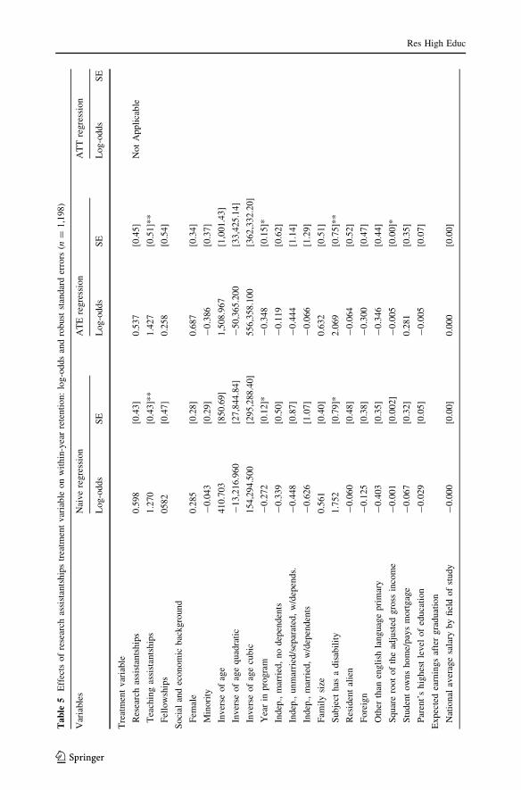
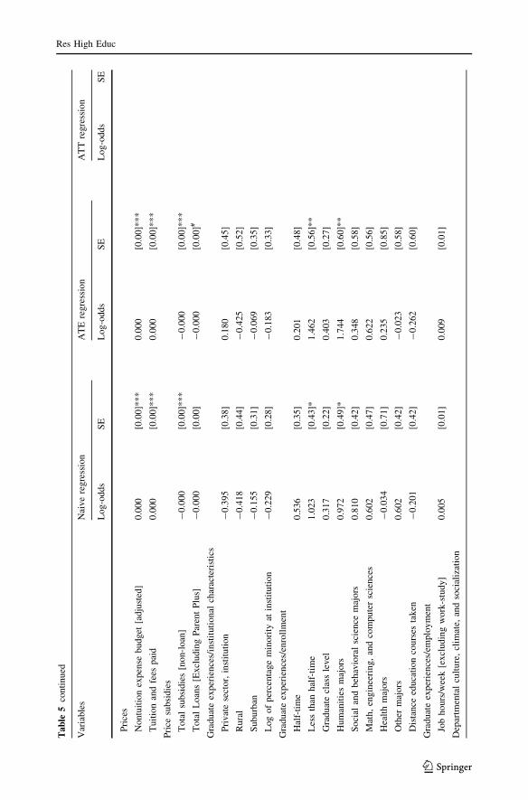
Research Assistantships
The logistic naive regression models indicate that while there appears to be a positive
relationship between research assistantships and within-year retention among Ph.D. stu-
dents, this result was statistically non-significant (see Table 5). While Ph.D. students who
have a research assistantship have a higher probability of being retained in comparison to
Ph.D. students who do not have either form of fellowship or assistantships, the general
relationship is not significantly different from the null. Controlling for selection bias, the
Average Treatment Effect model indicates that research assistants are slightly more likely
to experience within-year retention, although it remains statistically non-significant. This
particular result does indicate that the naive logistic regression model does slightly
overestimate the relationship. The two models do suggest that research assistants on
average do not appear to be retained at significant levels greater than their peers. While it is
likely that the within-year retention outcome during any academic year in a graduate
student’s career is not likely to be an important outcome for Ph.D. research assistants, it
remains important to continue to monitor and understand any potential changes to these
trends that may merit further investigation.
Fellowships
The naive logistic regression model results indicate there is a slightly positive though non-
significant relationship between fellowships and within-year retention (see Table 6). This
non-significant finding at first glance is unexpected. It was expected that Ph.D. fellows
would have a higher probability of retention than their Ph.D. peers who do not have either a
fellowship or assistantship. Controlling for selection bias, however, changes the effect of
fellowships from non-significance to marginal significance. This finding indicates that the
naive logistic regression model grossly underestimates the relationship. This finding
illustrates the importance of applying propensity score methods in higher education
research. Whereas the naive logistic regression model was not able to uncover the rela-
tionship, the Average Treatment Effect model results indicated that for functionally
equivalent groups, Ph.D. students on average are likely to have a higher probability of
within-year retention if they are on a fellowship. This finding is more consistent with
general conclusions that having a fellowship or assistantship improves the odds of reten-
tion. Additionally, the Average Treatment Effect on the Treated, which compares Ph.D.
Fellows with Ph.D. students who should have received a Fellowship but did not, indicates
that the mere act of participating in a Fellowship does increase the likelihood of experi-
encing within-year retention.
Debt-to-Price Ratio
The logistic naive regression model results indicate that there is no significant relationship
between the debt-to-price ratio, which represents how much indebtedness in relation to
tuition and fees paid a Ph.D. student is carrying on within-year retention (see Table 7).
After preforming checks for imbalance, we found that there was a sizable imbalance in the
debt-to-price ratio for both low debt and high debt groups; therefore, we could not proceed
Res High Educ
123
Ta
ble
5E
ffec
tso
fre
sear
chas
sist
ants
hip
str
eatm
ent
var
iab
leo
nw
ith
in-y
ear
rete
nti
on
:lo
g-o
dd
san
dro
bu
stst
andar
der
rors
(n=
1,1
98
)
Var
iable
sN
aive
regre
ssio
nA
TE
regre
ssio
nA
TT
regre
ssio
n
Lo
g-o
dd
sS
EL
og
-od
ds
SE
Lo
g-o
dd
sS
E
Tre
atm
ent
var
iab
le
Res
earc
has
sist
ants
hip
s0
.598
[0.4
3]
0.5
37
[0.4
5]
No
tA
pp
lica
ble
Tea
chin
gas
sist
ants
hip
s1
.270
[0.4
3]*
*1
.427
[0.5
1]*
*
Fel
low
ship
s0582
[0.4
7]
0.2
58
[0.5
4]
So
cial
and
eco
no
mic
bac
kg
roun
d
Fem
ale
0.2
85
[0.2
8]
0.6
87
[0.3
4]
Min
ori
ty-
0.0
43
[0.2
9]
-0
.386
[0.3
7]
Inv
erse
of
age
41
0.7
03
[85
0.6
9]
1,5
08
.96
7[1
,00
1.4
3]
Inv
erse
of
age
qu
adra
tic
-1
3,2
16
.96
0[2
7,8
44
.84]
-5
0,3
65
.20
0[3
3,4
25
.14
]
Inv
erse
of
age
cub
ic1
54
,29
4.5
00
[29
5,2
88
.40
]5
56
,35
8.1
00
[36
2,3
32
.20
]
Yea
rin
pro
gra
m-
0.2
72
[0.1
2]*
-0
.348
[0.1
5]*
Ind
ep.,
mar
ried
,n
od
epen
den
ts-
0.3
39
[0.5
0]
-0
.119
[0.6
2]
Ind
ep.,
un
mar
ried
/sep
arat
ed,
w/d
epen
ds.
-0
.44
8[0
.87
]-
0.4
44
[1.1
4]
Ind
ep.,
mar
ried
,w
/dep
end
ents
-0
.62
6[1
.07
]-
0.0
66
[1.2
9]
Fam
ily
size
0.5
61
[0.4
0]
0.6
32
[0.5
1]
Su
bje
cth
asa
dis
abil
ity
1.7
52
[0.7
9]*
2.0
69
[0.7
5]*
*
Res
iden
tal
ien
-0
.06
0[0
.48
]-
0.0
64
[0.5
2]
Fo
reig
n-
0.1
25
[0.3
8]
-0
.300
[0.4
7]
Oth
erth
anen
gli
shla
ng
uag
ep
rim
ary
-0
.40
3[0
.35
]-
0.3
46
[0.4
4]
Sq
uar
ero
ot
of
the
adju
sted
gro
ssin
com
e-
0.0
01
[0.0
02]
-0
.005
[0.0
0]*
Stu
den
to
wn
sh
om
e/pay
sm
ort
gag
e-
0.0
67
[0.3
2]
0.2
81
[0.3
5]
Par
ent’
shig
hes
tle
vel
of
educa
tion
-0
.02
9[0
.05
]-
0.0
05
[0.0
7]
Ex
pec
ted
earn
ing
saf
ter
gra
du
atio
n
Nat
ional
aver
age
sala
ryby
fiel
do
fst
udy
-0
.00
0[0
.00
]0
.000
[0.0
0]
Res High Educ
123
Ta
ble
5co
nti
nu
ed
Var
iable
sN
aive
regre
ssio
nA
TE
regre
ssio
nA
TT
regre
ssio
n
Lo
g-o
dd
sS
EL
og
-od
ds
SE
Lo
g-o
dd
sS
E
Pri
ces
Nontu
itio
nex
pen
sebudget
[adju
sted
]0.0
00
[0.0
0]*
**
0.0
00
[0.0
0]*
**
Tu
itio
nan
dfe
esp
aid
0.0
00
[0.0
0]*
**
0.0
00
[0.0
0]*
**
Pri
cesu
bsi
die
s
To
tal
sub
sid
ies
[no
n-l
oan
]-
0.0
00
[0.0
0]*
**
-0
.000
[0.0
0]*
**
To
tal
Lo
ans
[Ex
clu
din
gP
aren
tP
lus]
-0
.00
0[0
.00
]-
0.0
00
[0.0
0]#
Gra
duat
eex
per
ience
s/in
stit
uti
onal
char
acte
rist
ics
Pri
vat
ese
cto
r,in
stit
uti
on
-0
.39
5[0
.38
]0
.180
[0.4
5]
Ru
ral
-0
.41
8[0
.44
]-
0.4
25
[0.5
2]
Su
bu
rban
-0
.15
5[0
.31
]-
0.0
69
[0.3
5]
Log
of
per
centa
ge
min
ori
tyat
inst
ituti
on
-0
.22
9[0
.28
]-
0.1
83
[0.3
3]
Gra
du
ate
exp
erie
nce
s/en
roll
men
t
Hal
f-ti
me
0.5
36
[0.3
5]
0.2
01
[0.4
8]
Les
sth
anh
alf-
tim
e1
.023
[0.4
3]*
1.4
62
[0.5
6]*
*
Gra
du
ate
clas
sle
vel
0.3
17
[0.2
2]
0.4
03
[0.2
7]
Hum
anit
ies
maj
ors
0.9
72
[0.4
9]*
1.7
44
[0.6
0]*
*
So
cial
and
beh
avio
ral
scie
nce
maj
ors
0.8
10
[0.4
2]
0.3
48
[0.5
8]
Mat
h,
eng
inee
rin
g,
and
com
pu
ter
scie
nce
s0
.602
[0.4
7]
0.6
22
[0.5
6]
Hea
lth
maj
ors
-0
.03
4[0
.71
]0
.235
[0.8
5]
Oth
erm
ajo
rs0
.602
[0.4
2]
-0
.023
[0.5
8]
Dis
tance
educa
tion
cours
esta
ken
-0
.20
1[0
.42
]-
0.2
62
[0.6
0]
Gra
duat
eex
per
ience
s/em
plo
ym
ent
Job
ho
urs
/wee
k[e
xcl
udin
gw
ork
-stu
dy
]0
.005
[0.0
1]
0.0
09
[0.0
1]
Dep
artm
enta
lcu
lture
,cl
imat
e,an
dso
cial
izat
ion
Res High Educ
123
Ta
ble
5co
nti
nu
ed
Var
iable
sN
aive
regre
ssio
nA
TE
regre
ssio
nA
TT
regre
ssio
n
Lo
g-o
dd
sS
EL
og
-od
ds
SE
Lo
g-o
dd
sS
E
Pro
gra
msi
zeq
uar
tile
-0
.03
7[0
.15
]*-
0.3
15
[0.1
6]*
95
thP
erce
nti
lere
sear
chac
tiv
ity
-0
.01
1[0
.00
]**
-0
.012
[0.0
0]*
*
95
thP
erce
nti
lest
ud
ent
sup
po
rt&
ou
tco
mes
0.0
15
[0.0
0]*
**
0.0
16
[0.0
0]*
**
95
thP
erce
nti
led
iver
sity
-0
.00
2[0
.00
]-
0.0
01
[0.0
0]
Const
ant
-3
.77
0[8
.54
]-
15
.83
9[9
.94
]
#p\
0.1
0;
*p\
0.0
5;
**
p\
0.0
1;
**
*p\
0.0
01
Res High Educ
123
Tab
le6
Eff
ects
of
fell
ow
ship
str
eatm
ent
var
iab
leo
nw
ith
in-y
ear
rete
nti
on
:lo
g-o
dd
san
dro
bu
stst
and
ard
erro
rs(n
=1
,198
)
Var
iab
les
Nai
ve
reg
ress
ion
AT
Ere
gre
ssio
nA
TT
reg
ress
ion
Lo
g-o
dd
sS
EL
og
-od
ds
SE
Lo
g-o
dd
sS
E
Tre
atm
ent
var
iab
le
Fel
low
ship
s0.5
82
[0.4
7]
0.9
12
[0.4
8]#
1.3
56
[0.7
8]#
Tea
chin
gas
sist
ants
hip
s1.2
70
[0.4
3]*
*1.8
94
[0.5
8]*
**
2.0
412.0
41
[0.9
2]*
Res
earc
has
sist
ants
hip
s0
.598
[0.4
3]
1.2
48
[0.5
2]
1.3
42
[0.8
3]
So
cial
and
eco
no
mic
bac
kg
roun
d
Fem
ale
0.2
85
[0.2
8]
-0
.267
[0.3
9]
-0
.73
8[0
.49
]
Min
ori
ty-
0.0
43
[0.2
9]
0.2
21
[0.3
3]
0.1
70
[0.5
2]
Inv
erse
of
age
41
0.7
03
[85
0.6
9]
1,6
54
.485
[1,1
26.7
0]
92
6.4
9[2
,19
3.1
6]
Inv
erse
of
age
qu
adra
tic
-1
3,2
16
.96
0[2
7,8
44
.84]
-5
6,6
09
.10
0[3
6,8
39
.59
]-
39
,66
4.3
50
[68
,82
0.0
8]
Inv
erse
of
age
cub
ic1
54
,29
4.5
00
[29
5,2
88
.40
]6
45
,12
1.8
00
[39
1,4
41
.40
]#5
29
,33
6.9
00
[70
3,5
81
.90
]
Yea
rin
pro
gra
m-
0.2
72
[0.1
2]*
-0
.466
[0.1
6]*
*-
0.8
05
[0.2
4]*
**
Ind
ep.,
mar
ried
,n
od
epen
den
ts-
0.3
39
[0.5
0]
0.5
12
[0.5
5]
1.1
45
[0.9
6]
Ind
ep.,
un
mar
ried
/sep
arat
ed,
w/d
epen
ds.
-0
.448
[0.8
7]
1.1
73
[1.2
7]
0.7
87
[1.9
0]
Ind
ep.,
mar
ried
,w
/dep
end
ents
-0
.626
[1.0
7]
0.6
78
[1.0
6]
2.2
80
[2.0
8]
Fam
ily
size
0.5
61
[0.4
0]
-0
.049
[0.3
7]
-0
.64
5[0
.74
]
Su
bje
cth
asa
dis
abil
ity
1.7
52
[0.7
9]*
2.2
70
[0.9
0]*
5.2
85
[1.5
1]*
**
Res
iden
tal
ien
-0
.060
[0.4
8]
0.7
00
[0.6
5]
-0
.20
3[1
.27
]
Fo
reig
n-
0.1
25
[0.3
8]
-0
.075
[0.4
4]
-0
.20
5[0
.64
]
Oth
erth
anen
gli
shla
ngu
age
pri
mar
y-
0.4
03
[0.3
5]
-0
.743
[0.4
3]#
-0
.38
0[0
.72
]
Sq
uar
ero
ot
of
the
adju
sted
gro
ssin
com
e-
0.0
01
[0.0
0]
-0
.001
[0.0
0]
0.0
01
[0.0
0]
Stu
den
to
wn
sh
om
e/pay
sm
ort
gag
e-
0.0
67
[0.3
2]
0.3
18
[0.3
8]
0.9
89
[0.7
6]
Par
ent’
sh
igh
est
lev
elo
fed
uca
tio
n0
.029
[0.0
5]
-0
.063
[0.0
6]
-0
.03
2[0
.11
]
Ex
pec
ted
earn
ing
saf
ter
gra
du
atio
n
Nat
ion
alav
erag
esa
lary
by
fiel
do
fst
ud
y-
0.0
00
[0.0
0]
-0
.000
[0.0
0]
-0
.00
0[0
.00
]#
Res High Educ
123
Tab
le6
con
tin
ued
Var
iab
les
Nai
ve
reg
ress
ion
AT
Ere
gre
ssio
nA
TT
reg
ress
ion
Lo
g-o
dd
sS
EL
og
-od
ds
SE
Lo
g-o
dd
sS
E
Pri
ces
Nontu
itio
nex
pen
sebudget
[adju
sted
]0.0
00
[0.0
0]*
**
0.0
00
[0.0
0]*
*0.0
00
[0.0
0]#
Tu
itio
nan
dfe
esp
aid
0.0
00
[0.0
0]*
**
0.0
00
[0.0
0]*
**
0.0
00
[0.0
0]*
**
Pri
cesu
bsi
die
s
To
tal
sub
sid
ies
[no
n-l
oan
]-
0.0
00
[0.0
0]*
**
-0
.000
[0.0
0]*
**
-0
.00
0[0
.00
]*
To
tal
loan
s[e
xcl
udin
gp
aren
tp
lus]
-0
.000
[0.0
0]
-0
.000
[0.0
0]
0.0
00
[0.0
0]
Gra
duat
eex
per
ience
s/in
stit
uti
onal
char
acte
rist
ics
Pri
vat
ese
cto
r,in
stit
uti
on
-0
.395
[0.3
8]
-0
.257
[0.4
7]
0.0
35
[0.6
5]
Ru
ral
-0
.418
[0.4
4]
0.1
23
[0.4
9]
1.0
79
[0.8
6]
Su
bu
rban
-0
.155
[0.3
1]
0.5
80
[0.4
2]
0.9
46
[0.6
2]
Lo
go
fp
erce
nta
ge
min
ori
tyat
inst
itu
tio
n-
0.2
29
[0.2
8]
0.1
38
[0.3
5]
0.8
22
[0.5
8]
Gra
du
ate
exp
erie
nce
s/en
roll
men
t
Hal
f-ti
me
0.5
36
[0.3
5]
0.5
17
[0.4
3]
0.9
57
[0.6
6]
Les
sth
anh
alf-
tim
e1
.023
[0.4
3]*
0.8
18
[0.4
2]*
0.6
12
[0.8
5]
Gra
du
ate
clas
sle
vel
0.3
17
[0.2
2]
0.9
06
[0.3
1]*
*1
.435
[0.4
2]*
**
Hu
man
itie
sm
ajo
rs0
.972
[0.4
9]*
-0.0
14
[0.5
6]
-0
.76
0[0
.76
]
So
cial
and
beh
avio
ral
scie
nce
maj
ors
0.8
10
[0.4
2]#
1.5
89
[0.5
5]*
*2
.153
[0.8
4]*
*
Mat
h,
engin
eeri
ng,
and
com
pute
rsc
ience
s0.6
02
[0.4
7]
0.5
24
[0.5
3]
1.7
59
[0.8
5]*
Hea
lth
maj
ors
-0
.034
[0.7
1]
-0
.022
[0.8
2]
0.7
58
[1.7
7]
Oth
erm
ajo
rs0
.201
[0.4
2]
-0
.694
[0.5
1]
-0
.54
0[0
.64
]
Dis
tance
educa
tion
cours
esta
ken
-0
.315
[0.4
2]
-1
.029
[0.5
2]*
-1
.55
4[0
.97
]
Gra
du
ate
exp
erie
nce
s/em
plo
ym
ent
Job
ho
urs
/wee
k[e
xcl
ud
ing
wo
rk-s
tud
y]
0.0
05
[0.0
1]
0.0
04
[0.0
1]
0.0
03
[0.0
2]
Dep
artm
enta
lcu
lture
,cl
imat
e,an
dso
cial
izat
ion
Res High Educ
123
Tab
le6
con
tin
ued
Var
iab
les
Nai
ve
reg
ress
ion
AT
Ere
gre
ssio
nA
TT
reg
ress
ion
Lo
g-o
dd
sS
EL
og
-od
ds
SE
Lo
g-o
dd
sS
E
Pro
gra
msi
zeq
uar
tile
-0
.367
[0.1
5]*
-0
.466
[0.1
8]*
*-
0.5
40
0.5
40
[0.3
0]#
95th
Per
centi
lere
sear
chac
tivit
y-
0.0
11
[0.0
0]*
*-
0.0
19
[0.0
1]*
**
-0
.02
7[0
.01
]**
*
95
thP
erce
nti
lest
ud
ent
sup
po
rt&
ou
tco
mes
0.0
15
[0.0
0]*
**
0.0
07
[0.0
0]
0.0
04
[0.0
1]
95
thP
erce
nti
led
iver
sity
-0
.002
[0.0
0]
-0
.002
[0.0
0]
0.0
01
[0.0
1]
Co
nst
ant
-3
.770
[8.5
4]
-1
4.1
77
[11
.06]
-5
.55
3[2
2.4
5]
#p\
0.1
0;
*p
\0
.05;
**
p\
0.0
1;
**
*p
\0
.001
Res High Educ
123
Ta
ble
7E
ffec
tso
fd
ebt-
to-p
rice
rati
otr
eatm
ent
on
wit
hin
-yea
rre
ten
tio
n:
log
-od
ds
and
rob
ust
stan
dar
der
rors
(n=
1,1
98
)
Var
iable
sN
aive
regre
ssio
nA
TE
regre
ssio
nA
TT
regre
ssio
n
Lo
g-o
dd
sS
EL
og
-od
ds
SE
Lo
g-o
dd
sS
E
Tre
atm
ent
var
iab
le
Gra
du
ate
deb
to
ver
tuit
ion
&fe
es0
.092
[0.2
6]
No
tA
pp
lica
ble
-0
.021
[0.2
9]
So
cial
and
eco
no
mic
bac
kg
roun
d
Fem
ale
0.1
05
[0.2
6]
0.1
57
[0.3
3]
Min
ori
ty-
0.0
80
[0.2
6]
-0
.261
[0.3
0]
Inv
erse
of
age
-1
38
.72
2[7
91
.28
]-
38
1.0
66
[1,1
64.5
8]
Inv
erse
of
age
qu
adra
tic
4,3
42
.440
[25
,777
.36
]5
,581
.08
[37
,237
.77]
Inv
erse
of
age
cub
ic-
26
,36
1.4
80
[27
2,5
18
.60
]2
4,0
99
.05
0[3
86
,56
8.5
0]
Yea
rin
pro
gra
m-
0.3
39
[0.1
2]*
*-
0.6
81
[0.1
8]*
**
Ind
ep.,
mar
ried
,n
od
epen
den
ts-
0.5
42
[0.5
0]
-0
.551
[0.6
3]
Ind
ep.,
un
mar
ried
/sep
arat
ed,
w/d
epen
ds.
-0
.15
5[0
.75
]-
0.5
30
[1.0
0]
Ind
ep.,
mar
ried
,w
/dep
end
ents
-0
.89
3[0
.94
]-
0.9
60
[1.2
7]
Fam
ily
size
0.6
25
[0.3
5]#
0.8
23
[0.4
7]#
Su
bje
cth
asa
dis
abil
ity
1.7
94
[0.7
6]*
3.7
75
[1.1
2]*
**
Res
iden
tal
ien
-0
.11
4[0
.46
]0
.679
[0.6
6]
Fo
reig
n0
.300
[0.3
8]
1.4
18
[0.5
7]*
Oth
erth
anen
gli
shla
ngu
age
pri
mar
y-
0.1
97
[0.3
2]
-0
.961
[0.4
0]*
Sq
uar
ero
ot
of
the
adju
sted
gro
ssin
com
e-
0.0
02
[0.0
0]
-0
.003
[0.0
0]
Stu
den
to
wn
sh
om
e/pay
sm
ort
gag
e-
0.0
61
[0.2
9]
-0
.120
[0.3
5]
Par
ent’
shig
hes
tle
vel
of
educa
tion
-0
.02
0[0
.05
]-
0.0
73
[0.0
6]
Ex
pec
ted
earn
ing
saf
ter
gra
du
atio
n
Nat
ion
alav
erag
esa
lary
by
fiel
do
fst
ud
y-
0.0
00
[0.0
0]
-0
.000
[0.0
0]
Res High Educ
123
Tab
le7
con
tin
ued
Var
iable
sN
aive
regre
ssio
nA
TE
regre
ssio
nA
TT
regre
ssio
n
Lo
g-o
dd
sS
EL
og
-od
ds
SE
Lo
g-o
dd
sS
E
Pri
ces
Nontu
itio
nex
pen
sebudget
[adju
sted
]0.0
00
[0.0
0]*
*0.0
00
[0.0
0]*
Pri
cesu
bsi
die
s
To
tal
sub
sid
ies
[no
n-l
oan
]-
0.0
00
[0.0
0]
-0
.000
[0.0
0]*
Pri
vat
ese
cto
r,in
stit
uti
on
0.9
99
[0.3
2]*
*0
.690
[0.4
0]#
Ru
ral
-0
.599
[0.4
0]
-1
.415
[0.4
7]*
*
Su
bu
rban
0.2
85
[0.2
8]
0.0
79
[0.3
6]
Log
of
per
centa
ge
min
ori
tyat
inst
ituti
on
-0
.291
[0.2
4]
-0
.125
[0.2
9]
Gra
duat
eex
per
ience
s/en
roll
men
t
Hal
f-ti
me
-0
.002
[0.3
1]
-0
.490
[0.3
7]
Les
sth
anh
alf-
tim
e0
.04
0[0
.39
]-
0.1
06
[0.5
4]
Gra
du
ate
clas
sle
vel
0.3
32
[0.2
0]#
1.0
75
[0.3
3]*
**
Hu
man
itie
sm
ajo
rs0
.67
9[0
.44
]1
.150
[0.5
6]*
So
cial
and
beh
avio
ral
scie
nce
maj
ors
0.6
51
[0.3
8]#
0.9
57
[0.5
2]#
Mat
h,
eng
inee
rin
g,
and
com
pu
ter
scie
nce
s0
.96
2[0
.44
]*1
.277
[0.7
3]#
Hea
lth
maj
ors
0.4
37
[0.6
6]
0.4
33
[0.8
6]
Oth
erm
ajo
rs0
.29
7[0
.39
]-
0.0
79
[0.5
2]
Dis
tance
educa
tion
cours
esta
ken
-0
.506
[0.3
9]
-0
.399
[0.4
9]
Gra
duat
eex
per
ience
s/em
plo
ym
ent
Job
ho
urs
/wee
k[e
xcl
ud
ing
wo
rk-s
tud
y]
-0
.002
[0.0
1]
0.0
00
[0.0
1]
Tea
chin
gas
sist
ants
hip
0.7
82
[0.3
8]*
0.7
12
[0.4
8]
Res
earc
has
sist
ants
hip
0.1
28
[0.3
7]
-0
.005
[0.5
0]
Res High Educ
123
Tab
le7
con
tin
ued
Var
iable
sN
aive
regre
ssio
nA
TE
regre
ssio
nA
TT
regre
ssio
n
Lo
g-o
dd
sS
EL
og
-od
ds
SE
Lo
g-o
dd
sS
E
Fel
low
ship
0.2
85
[0.2
9]
0.0
00
[0.4
8]
Dep
artm
enta
lcu
ltu
re,
clim
ate,
and
soci
aliz
atio
n
Pro
gra
msi
zeq
uar
tile
-0
.369
[0.1
3]*
*-
0.4
77
[0.1
7]*
*
95th
Per
centi
lere
sear
chac
tivit
y-
0.0
12
[0.0
0]*
**
-0
.014
[0.0
0]*
95
thP
erce
nti
lest
ud
ent
sup
po
rt&
ou
tco
mes
0.0
14
[0.0
0]*
**
0.0
11
[0.0
0]*
*
95
thP
erce
nti
led
iver
sity
-0
.001
[0.0
0]
0.0
01
[0.0
0]
Co
nst
ant
5.2
42
[7.9
4]
9.8
02
[12
.08
]
#p
\0
.10;
*p\
0.0
5;
**
p\
0.0
1;
**
*p\
0.0
01
Res High Educ
123
with an analysis of the Average Treatment Effect model. However, the Average Treatment
Effect on the Treated, which compares the high debt ratio Ph.D. students with those Ph.D.
students who should have a high debt ratio but do not, finds that the level of indebtedness
would have had no different effects for these Ph.D. students. In essence, whether or not a
Ph.D. student has a higher ratio of indebtedness would not have had a differing effect on
Ph.D. students’ likelihood of being retained.
Discussion and Interpretation of Results
Although past studies suggest that financial aid in general facilitates doctoral retention,
there is no consensus on the effects of different forms of aid on doctoral outcomes
(Mwenda 2010). On the one hand, some have argued that fellowships allow students to be
more focused and efficient towards degree completion and relieve students from the stress
of financing their education and so, these students tend to experience shorter trajectories
time to degree (Herzig 2004). Another positive outcome of fellowships is that by providing
students with financial resources and greater availability of time, they are more likely to
attend conferences and other professional development events (Mwenda 2010). Others
have mentioned that the positive effect of fellowships takes place mainly in the humanities
because students tend to embark on research in isolation and that in STEM fields, fel-
lowships are detrimental towards degree progress because they do not enable students’
ability to join research groups as it is the case with research assistantships. In STEM fields,
joining a research group is normally the foundation for dissertation work and the means for
proper socialization conducive of doctoral retention. Therefore, some argue that research
assistantships are the most effective financial support for doctoral completion, especially in
STEM fields (Ampaw and Jaeger 2012; Bair and Haworth 1999; Bowen and Rudenstine
1992). Some have argued that teachings assistantships are also positive by facilitating the
integration of students into the academic communities increasing contact with faculty and
peers, despite the lack of attention to research (Austin 2002; Girves and Wemmerus 1988;
faculty relationships can damper the positive effects of research assistantships. Qualitative
studies have demonstrated the importance of these relationships (Mwenda 2010), however,
Table 8 Treatment variable effects on within-year retention based on fully specified theoretical models fornaive regression models, average treatment effects models, and average treatment on the treated effectsmodels: log-odds and robust standard errors (n = 1,198)
Treatment variables Naive regression ATE ATT
Log-odds SE Log-odds SE Log-odds SE
1. Research assistantships 0.598 (.43) 0.537 (.45) Not applicablea
4. Debt-to-price 0.095 (.26) Not applicablea 0.021 (.29)
Reference category for the research assistantships, teaching assistantships, and fellowships models is Ph.D.students with no assistantships or fellowships
Reference category for all debt-to-price models is no debt or debt less than the price of attending graduateschool for a Ph.D
All models above included a vector of predictor variables as provided in Table 1 under the model column.They were listed as models 1, 2, 3, 4, and All
All model results including the control and balancing variables are available by request from the authors# p \ 0.10; *p \ 0.05; ** p \ 0.01;a The checks for covariate balance conducted after generating the propensity score weight indicated that theweight under the ATE treatment for Debt-to-Price and Research Assistantships did not balance the data wellenough to allow estimation of the regression results using propensity score weights
Res High Educ
123
quantitative accounts of this dimension are still lacking in the literature. This indicates a
need for including measures of student-advisor/faculty relationships in future quantitative
research. Despite the statistical efforts undertaken to control for selection bias on
observables, this finding serves as an example of the limitations that occur due to the
inability to control for unobservable, such as the student-advisor relationship. Also, it is
possible that research assistantships offer less financial stability given the fact that they are
normally part of research grants, which vary in duration and in some cases, suffer from
abrupt termination. In other words, research assistantships can be short-term and limited in
scope providing a greater sense of employment ambiguity to the Ph.D. student. Clearly, to
answer these questions, future research should further investigate the role of research
assistantships in doctoral retention.
Doctoral students are increasingly relying on loans to afford the price of attendance
(Hoffer et al. 2006). According to the National Science Foundation (NSF), 48 % of doctoral
graduates in 2009–2010 owed over $20,400 on average in education-related debt and 16 %
owed over $50,000 in combined undergraduate and graduate debt. However, to the best of
our knowledge, this is the first quantitative study investigating the role of debt on doctoral
retention. Gardner and Holley (2011) in a qualitative study tapped into the issue of loan debt
among doctoral students, indicating that ‘‘students had faith that the attainment of the doc-
toral degree would eventually mitigate these financial concerns, as they expected their
professional careers would bring financial stability to their lives’’ (p. 87). This attitude might
provide insights to the non-significance of debt in relation to price of attendance found in this
study, in that students are confident about their employability and earnings after graduation
to pay their loans and so, debt is not a central consideration for leaving the program. In fact,
debt might have the opposite effect to some students by motivating them to graduate, earn at
the expected level for Ph.D.’s in their field, and pay their loans. Thus, given the current levels
of debt of doctoral students and favorable labor market conditions, debt might not be a
critical factor in doctoral attrition. This finding does point to a need to monitor this effect as
more students enroll in Ph.D. programs with greater levels of debt. As a matter of policy
concern, it will be incumbent of institutions to be proactive in ensuring that Ph.D. students do
not take too much debt without understanding the potential consequences for indebtedness
on other important outcomes such as type of employment after degree completion. A perhaps
more relevant question might be related to the effects of debt on doctoral enrollment. As with
the case in undergraduate education, the prospect of high levels of debt my discourage
students with high debt aversion to enroll in doctoral programs.
This study shows that retention and the role of teaching assistantships, research assis-
tantships, fellowships, and debt manifest differently by field of study, gender, race/eth-
nicity, and immigration status. This study shows that the patterns associated with gender,
race/ethnicity, and immigration status varies dramatically by field of study. Therefore,
future studies, when possible, should not aggregate fields of study in their analysis.
Another notable theme is that the gender gap exists across fields and within racial/ethnic
groups except for a few exceptions among US Whites in the life sciences, humanities, and
social/behavioral sciences. In some instances, the gender gap favors females in some fields,
especially in health and life sciences. Asian foreigners, especially males, dominate the
math, engineering, and computer science fields. US minority students are significantly
underrepresented except for Asians in some fields. In general, minority women tend to
perform better than their male counterparts. Most notable is the fact that US Black males
are the most underrepresented group in all fields. These results support previous work
developing the concept of ‘‘rejection of academic careers’’ and the lack of feelings of
Res High Educ
123
belonging as common reasons for the underrepresentation of minorities in advanced
degrees (Glazer-Raymo 1999; Winkle-Wagner 2009).
As the higher education financial aid policy landscape continues to emphasize education
as a private good, student debt will continue to be a source of concern as it will likely have
differential effects by student demographics and field of study. Concomitantly, it is
expected that the federal government and institutions will continue to offer graduate as-
sistantships and fellowships to doctoral students. This study provides timely insights into
which of these financial strategies are likely to improve the already low doctoral retention
rates nationwide. To the best of our knowledge, this is the first quantitative study that
includes socialization variables in examining the role of various funding mechanisms in
doctoral retention using a national representative database. Given the essential role of the
experience within each academic unit in doctoral education, much more than in under-
graduate education, this study promises to shed light not only to the role of finances in
doctoral retention, but also to the role of academic integration and socialization in com-
bination to funding in doctoral outcomes. Clearly, future studies should examine the role of
the student-advisor/faculty relationship in doctoral retention as well as disaggregated data
by field of study, gender, race/ethnicity, and immigration status.
References
Ampaw, F. D., & Jaeger, A. J. (2012). Completing the three stages of doctoral education: An event historyanalysis. Research in Higher Education, 53, 640–660.
Austin, A. E. (2002). Preparing the next generation of faculty: graduate school as socialization to academiccareers. The Journal of Higher Education, 73(1), 94–122.
Bair, C. R. & Haworth, J.G. (1999). Doctoral student attrition and persistence: A metasynthesis of research.Paper presented at the annual meeting of the Association for the Study of Higher Education, SanAntonio, TX. (ERIC Document Reproduction Service No. ED437008).
Bowen, W. G., & Rudenstine, N. L. (1992). In pursuit of the Ph.D.. Princeton: Princeton University Press.Braskman, L., & Wergin, J. (1998). Forming new social partnerships. In W. Tierney (Ed.), The responsive
university: Restructuring for high performance (pp. 62–91). Baltimore: Johns Hopkins UniversityPress.
Burton, N. W., & Ramist, L. (2001). Predicting success in college: SAT studies of classes graduating since1980. New York: College Entrance Examination Board.
College Board. (2011). Trends in student aid. (Trends in Higher Education Series). Washington: Author.Cominole, M., Riccobono, J., Siegel, P., & Caves, L. (2010). 2007–08 National Postsecondary Student Aid
Study (NPSAS:08) Full-scale Methodology Report (NCES 2011-188). Washington: US Department ofEducation, National Center for Education Statistics.
DesJardins, S. L., & McCall, B. P. (2010). Simulating the effects of financial aid packages on collegestudent stop out, reenrollment spells, and graduation chances. Review of Higher Education, 33(4),513–541.
Dowd, A. C. (2008). Dynamic interactions and intersubjectivity: Challenges to causal modeling in studies ofcollege student debt. Review of Educational Research, 78(2), 232–259.
Gardner, S. K. (2009). Student and faculty attributions of attrition in high and low-completing US doctoralprograms. Higher Education, 58, 97–112.
Gardner, S. K., & Barnes, B. J. (2007). Graduate student involvement: Socialization for the professionalrole. The Journal of College Student Development, 48, 369–387.
Gardner, S. K., & Holley, K. A. (2011). Those invisible barriers are real: The progression of first-generationstudents through doctoral education. Equity and Excellence in Education, 44(1), 77–92.
Gardner, S. K., & Mendoza, P. (2010). On becoming a scholar: Socialization and development in doctoraleducation. Sterling: Stylus.
Girves, J. E., & Wemmerus, V. (1988). Developing models of graduate student degree progress. The Journalof Higher Education, 59(2), 163–189.
Glazer-Raymo, J. (1999). Shattering the myths: Women in academe. Baltimore: Johns Hopkins UniversityPress.
Res High Educ
123
Golde, C. M. (2000). Should I stay or should I go? Student descriptions of the doctoral attrition process.Review of Higher Education, 23(2), 119–227.
Golde, C. M. (2005). The role of the department and discipline in doctoral student attrition: lessons fromfour departments. Journal of Higher Education, 76, 669–700.
Guo, S., & Fraser, W. M. (2010). Propensity score analysis: Statistical methods and applications. ThousandOaks: Sage.
Gururaj, S., Heilig, J. V., & Somers, P. (2010). Graduate student persistence: Evidence from three decades.Journal of Student Financial Aid, 40(1), 31–46.
Hahs-Vaughn, D. L., & Onwuegbuzie, A. J. (2006). Estimating and using propensity score analysis withcomplex samples. The Journal of Experimental Education, 73(1), 31–65.
Herzig, A. H. (2004). Becoming mathematicians: Women and students of color choosing and leavingdoctoral mathematics. Review of Educational Research, 74(2), 171–214.
Hoffer, T. B., Welch, V., Webber, K., Williams, K., Lisek, B., Hess, M., et al. (2006). Doctorate recipientsfrom United States universities: Summary report 2005. Chicago: National Opinion Research Center.
Hossler, D., Ziskin, M., Gross, J. P., Kim, S., & Cekic, O. (2009). Student aid and its role in encouragingpersistence. Higher education: Handbook of theory and research (pp. 389–425). Netherlands:Springer.
Kim, D. (2007). The effect of loans on students’ degree attainment: differences by student and institutionalcharacteristics. Harvard Educational Review, 77(1), 64–100.
Kim, D., & Otts, C. (2010). The effect of loans on time to doctorate degree: Differences by race/ethnicity,field of study, and institutional characteristics. Journal of Higher Education, 81(1), 1–32.
Little, R. J. A., & Rubin, D. B. (2002). Statistical analysis with missing data (2nd ed.). Hoboken: Wiley.Long, J. S. (1997). Regression models for categorical and limited dependent variables. Thousand Oaks:
SAGE.Lovitts, B. E. (2001). Leaving the ivory tower: The causes and consequences of departure from doctoral
study. Lanham: Rowman & Littlefield.Malcolm, L. E., & Dowd, A. C. (2012). The impact of undergraduate debt on the graduate school enrollment
of STEM baccalaureates. The Review of Higher Education, 35(2), 265–306.Mendoza, P. (2007). Academic capitalism and doctoral student socialization: A case study. Journal of
Higher Education, 78(1), 71–96.Morgan, S. L., & Winship, C. (2007). Counterfactuals and causal inference: Methods and principles for
social science research. New York: Cambridge University Press.Murnane, R. J., & Willett, J. B. (2011). Methods matter: Improving causal inference in educational and
social science research. New York: Oxford University Press.Mwenda, M. N. (2010). Underrepresented minority students in STEM doctoral programs: The role of
financial support and relationships with faculty and peers. Dissertation, University of Iowa.National Science Board. (2012). Science and Engineering Indicators 2012. Arlington: National Science
Foundation (NSB 12-01).Nettles, M. T., & Millett, C. M. (2006). Three magic letters: Getting to Ph.D (1st ed.). Baltimore: The Johns
Hopkins University Press.Peduzzi, P., Concato, J., Kemper, E., Holford, T. R., & Feinstein, A. R. (1996). A simulation study of the
number of events per variable in logistic regression analysis. Journal of Clinical Epidemiology, 49,1372–1379.
Schafer, J. L., & Kang, J. (2008). Average causal effects from non-randomized studies: A practical guideand simulated example. Psychological Methods, 13(4), 279–313.
Schneider, B., Carnoy, M., Kilpatrick, J., Schmidt, W. H., & Shavelson, R. J. (2007). Estimating causaleffects using experimental and observational designs: A think tank white paper. Washington: AmericanEducational Research Association.
Shadish, W. R., Campbell, D. T., & Cook, T. D. (2002). Experimental and quasi-experimental designs forgeneralized causal inference. Boston: Houghton Mifflin.
Slaughter, S., Campbell, T., Hollernan, M., & Morgan, E. (2002). The ‘‘traffic’’ in graduate students:Graduate students as tokens of exchange between academe and industry. Science, Technology andHuman Values, 27(2), 282–313.
St. John, E. P., & Andrieu, S. C. (1995). The influence of price subsidies on within-year persistence bygraduate students. Higher Education, 29, 143–168.
Stata Press. (2011). Stata multiple imputation reference manual, release 12. College Station: Author.Tierney, W. (1992). Cultural leadership and the search for community. Liberal Education, 78(5), 16–21.Tinto, V. (1993). Leaving college: Rethinking the causes and cures of student attrition (2nd ed., p. 296).
Chicago: University of Chicago Press.
Res High Educ
123
Walker, G. E., Golde, C. M., Jones, L., Conklin Bueschel, A., & Hutchings, P. (2008). The formation ofscholars: Rethinking doctoral education for the twenty-first century. San Francisco: Jossey-Bass.
Weidman, J. C., Twale, D. J., & Stein, E. L. (2001). Socialization of graduate and professional students inhigher education: A perilous passage?. San Francisco: Jossey-Bass.
Wendler, C., Bridgeman, B., Cline, F., Millett, C., Rock, J., Bell, N., et al. (2010). The path forward: Thefuture of graduate education in the United States. Council of Graduate School: Educational TestingService.
Winkle-Wagner, R. (2009). The unchosen me: Race, gender, and identity among Black women in college.Baltimore: The Johns Hopkins University Press.