1 Women, confidence, and financial literacy Tabea Bucher-Koenen Max-Planck-Institute for Social Law and Social Policy and Netspar Rob Alessie University of Groningen and Netspar Annamaria Lusardi George Washington School of Business, NBER and Netspar and Maarten van Rooij* De Nederlandsche Bank and Netspar February 2016 Abstract The literature documents robust evidence of a gender gap in financial literacy: Women consistently show lower levels of financial literacy than men. We have devised two surveys to investigate whether this gender gap is the result of lack of knowledge or lack of confidence. We show that women are less confident in their knowledge than men. Specifically, women disproportionately answer financial knowledge questions with “do not know,” even when they know the correct answer. We develop an empirical strategy to consistently estimate whether respondents know the correct answer. Using this improved metric for knowledge, we show that the gender gap diminishes by about half but does not disappear. Using this alternative measure of financial literacy, we show that financial knowledge continues to be an important predictor of financial behavior, such as participation in the stock market. Keywords: financial literacy, gender difference, financial decision-making, measurement error JEL code: C81, D91 * Tabea Bucher-Koenen, Munich Center for the Economics of Aging at the Max-Planck-Institute for Social Law and Social Policy, Amalienstr. 33, 80799 Munich, Germany ([email protected]), Rob J.M. Alessie, School of Economics and Business, University of Groningen, P.O. Box 800, 9700 AV, Groningen ([email protected]),), Annamaria Lusardi, The George Washington University School of Business, Duquès Hall, Suite 450E, Washington D.C. ([email protected]), Maarten C.J. van Rooij, Economics & Research Division, De Nederlandsche Bank, P.O. Box 98, 1000 AB, Amsterdam ([email protected]). The authors wish to thank Martin Brown for suggestions and comments and participants of the Annual Meeting of the Neuroeconomic Society (Bonn 2013) and the Annual Conference of the European Economics Association (Toulouse 2014) for useful comments. They also gratefully acknowledge financial support from the European Investment Bank Institute through its EIBURS initiative. The findings, interpretations and conclusions presented in this article are entirely those of the authors and should not be attributed in any manner to the European Investment Bank or its Institute or the De Nederlandsche Bank. Any errors are solely the authors’ responsibility.
Transcript
1
Women, confidence, and financial literacy
Tabea Bucher-Koenen
Max-Planck-Institute for Social Law and Social Policy and Netspar
Rob Alessie
University of Groningen and Netspar
Annamaria Lusardi
George Washington School of Business, NBER and Netspar
and
Maarten van Rooij*
De Nederlandsche Bank and Netspar
February 2016
Abstract
The literature documents robust evidence of a gender gap in financial literacy: Women
consistently show lower levels of financial literacy than men. We have devised two surveys to
investigate whether this gender gap is the result of lack of knowledge or lack of confidence. We
show that women are less confident in their knowledge than men. Specifically, women
disproportionately answer financial knowledge questions with “do not know,” even when they
know the correct answer. We develop an empirical strategy to consistently estimate whether
respondents know the correct answer. Using this improved metric for knowledge, we show that
the gender gap diminishes by about half but does not disappear. Using this alternative measure
of financial literacy, we show that financial knowledge continues to be an important predictor
of financial behavior, such as participation in the stock market.
Women show consistently low levels of financial literacy. They are less likely to answer simple
financial knowledge questions correctly, they are more likely to answer “do not know” to those
questions, and they rate themselves lower than men in terms of self-assessed financial literacy.
This is true across countries and measures of financial knowledge, as well as across socio-
demographic characteristics (see, e.g., Bucher-Koenen, Lusardi, Alessie, and Van Rooij, 2014,
and OECD, 2013, for overviews). It is particularly striking that financial literacy levels seem to
be low among young women who are well educated and have strong labor market attachment.
Even women from an elite American college show considerable lack of financial expertise
(Mahdavi and Horton, 2014).
The persistent gender gap in financial literacy may be the result of women feeling less confident
in their financial knowledge. There is ample evidence that women are less confident than men,
in particular in situations related to finance (see, e.g., Beyer, 1990; Barber and Odean, 2001).
Some studies indicate that while men appear to be over-confident, women seem under-
confident (see Dahlbom et al., 2011). In the context of financial knowledge, Chen and Volpe
(2002) find that female college students are less confident and enthusiastic about financial
topics. Webster and Ellis (1996) provide evidence that, even among financial experts, women
show lower self-confidence in financial analyses compared to men.
This is consistent with the evidence provided by the self-assessed knowledge responses in our
surveys, which shows that some of the women who respond with at least one “do not know”
give themselves high knowledge assessments (see Bucher-Koenen, Lusardi, Alessie, and Van
Rooij, 2014). Thus, irrespective of the fact that they are inclined not to answer specific financial
literacy questions, women still consider themselves financially competent. So the central
question is the following: do those (women) who answer “do not know” know the answer but
lack confidence in their knowledge?
In order to investigate this question, we design a simple experiment with the Dutch DNB
Household Survey (DHS). The objective is to understand what drives the gender gap in
financial literacy and in particular what drives the gender difference in the “do not know”
responses. Our first hypothesis is that by offering a “do not know” option, we introduce noise
in that other characteristics (specifically gender) that affect the propensity to reply with “do not
3
know” enter the literacy measure. Specifically, we ran two surveys among the DHS respondents
that were conducted six weeks apart from one another. In the first survey, we ask respondents
the financial literacy questions with the option of a “do not know” reply as part of the multiple
choice answers. We then follow these respondents over time and ask the same knowledge
questions again, but this time taking away the “do not know” option and adding a follow-up
question to assess how confident respondents are in their answers. This new set of data will
allow us to dissect the answers to the financial literacy questions and examine the drivers of
women’s “do not know” responses. Our hypothesis is that by improving the measurement of
financial literacy, we can estimate the effect of financial literacy on financial behavior more
precisely and eliminate some of the bias plaguing those estimates.
The central contribution of this paper is that we develop a strategy, based on two survey waves,
to consistently estimate whether the respondents truly know the correct answers to the financial
literacy questions. In doing so, we improve the measurement of financial literacy and can solve
some of the problems existing in the current literature. Our main result is that women know less
than men but they know more than they think they know. That is, if we take away the “do not
know” option, women are very likely to give correct responses to the financial literacy
questions. At the same time, women appear to be less confident in their answers. Thus, the
gender gap in financial literacy is driven by both lower knowledge and lack of confidence. Our
results have two implications. Firstly, there should be financial education programs that are
tailored to women. They should convey information as well as instill confidence in women of
their knowledge and decision-making abilities. The second implication is methodological:
when measuring financial literacy in surveys, researchers have to consider systematic bias
induced by different response behavior. We suggest alternative strategies to improve the
measurement of financial literacy.
The paper is organized as follows: in the next section we present the data and the experimental
design. In section 3 we show descriptive results. In section 4 we propose a strategy for
measuring financial literacy if there are differences in confidence that are different across
gender. We explore different financial literacy measures in section 5 and present results for
financial behavior in section 6. In section 7 we present some robustness checks and in section
8 we provide concluding remarks.
4
2. The data
2.1 The CentERpanel
We use data from the CentERpanel to investigate financial literacy and confidence among a
representative set of Dutch-speaking households. The CentERpanel is an online household
panel run by CentERdata, a survey agency at Tilburg University. Participants without internet
connection are provided with the equipment necessary to participate in the survey.1 We include
all panel members who are household heads and their partners in the sample. Respondents are
age 18 and older. The data used in our study are collected between May and July 2012. We are
able to merge our data with the DNB Household Survey (DHS). The DHS is an annual survey
among the CentERpanel on income, assets and debt, work, health and economic and
psychological concepts related to savings behavior.
2.2 The experiment
The experimental design is as follows: We ask the same three quiz-like questions on financial
literacy to the same respondents twice (see Appendix A1 for the wording of the questions).2
When we ask the questions for the first time in May 2012 respondents are offered “do not know”
and “refuse to answer” options in the responses to the questions. When we ask the same
questions for the second time about six weeks later at the end of June/beginning of July 2012
those options are deleted; thus, respondents have to choose an answer for these questions. In
this survey, respondents are required to rate the confidence they have in their answer on a scale
from 1 (not confident at all) to 7 (completely confident) after each question.
2.3 The sample
In the first survey3 we have 1,748 participants and in the second survey we have 1,973
participants, including a refresher. For our main analysis we restrict the sample to the
respondents who participate in both waves. We allow both the household head and their partner
to participate, thus for a number of households we have two individual observations (and in the
regression analysis we compute standard errors which are clustered at the household level). In
1 For more information, see www.centerdata.nl. 2 These questions have been developed by Annamaria Lusardi and Olivia Mitchell and were first asked
to respondents of the American Health and Retirement Study in 2004 (Lusardi and Mitchell 2011a).
Since then they have been used widely to measure financial literacy in surveys around the world (see
Lusardi and Mitchell, 2011b, and the papers in special issues of the Journal of Pension Economics and
Finance, vol. 104, 2011 and Numeracy, vol. 6, 2013 for some examples). 3 In the paper, we will mention interchangeably first and second survey to mean May and July survey.
5
our empirical analysis, we drop respondents who did not complete the financial literacy surveys
(30 respondents; 1.35% of the initial raw sample). The reduced sample contains 1,532
respondents for all our analyses; 861 (56.2%) are men and 671 (43.8%) are women.4
Before we show our results, we need to discuss two important points based on the unrestricted,
i.e. unbalanced, sample:
1. Attrition: We test for attrition between the waves, conditional on financial literacy.
Specifically, we look at the average number of correct answers in the first wave and partition
the sample into those who participate only in the first wave and those who participate in both
waves. We do not find a systematic difference in the average financial literacy of those groups.
Thus, we conclude that respondents do not drop out systematically after the first survey because
they are uncomfortable with answering the financial literacy questions. The same is true for
attrition based on gender. Men and women both drop out after the first wave with equal
probability.
2. Learning: Since we ask the same questions twice to the same respondents within a six-week
period, one might be worried about learning effects. We can test for learning by comparing the
probability to give correct answers in the second wave for the refresher sample, who participate
only in the second wave, with the sample of respondents who participate in both waves. There
is no significant difference in the answering behavior of those two groups in the second week.
Thus, we feel confident that learning effects are not confounding our results.
3. Descriptive results
3.1 Comparing answers across waves
In table 1 we present the answers to all financial literacy questions for both the first and the
second survey separately for men and women.5
[Table 1 - Tabulation of literacy responses in wave 1 and 2 - about here]
In the May survey for the interest question, men report more correct answers than women
(91.9 % vs. 84.4%, see table 1 panel A). Thus the gender gap in giving the correct answer is
4 The sample used in the regression analyses may vary slightly due to missing values for some control
variables, especially when we merge our survey with the information from the DHS. 5 The statistics presented in this paper are not weighted. We also used sampling weights but found only
very small differences.
6
around 7.5 percentage points. Women are more often incorrect, but more importantly they
report a higher number of “do not know” (DK) answers. In the July survey we ask the same
question without the DK option. The number of correct answers increases significantly to
94.7% for men and 91.2% for women. The number of incorrect answers also increases.
However, overall the gender difference decreases to 3.5 percentage points. Note that the number
of refusals to answer is very limited. Hence, in the further analysis, we lump this category
together with the “do not know” responses. If we condition the answers of wave 2 on the wave
1 responses, it is of particular interest how accurate the wave 2 responses are for those who
stated “do not know” in wave 1 (see table 2). It appears that the majority of this group is able
to provide the correct answer when forced to provide an answer, which suggests that they are
not simply guessing the answer.6 Around 70% of both men and women who said “do not know”
in the first survey are able to correctly answer the interest question in the second survey.
[Table 2 - Tabulation of wave 2 responses conditional on wave 1 responses - about here]
The inflation question appears to be somewhat more difficult to answer. The number of correct
answers is lower and the gender gap is larger at more than 9 percentage points (see table 1 panel
B). Two thirds of the gender gap is driven by the DK’s, although the number of incorrect
answers is also somewhat higher among women. When forced to answer, the gender gap
diminishes from 9 to 6 percentage points. This is due to the fact that the group that provides a
DK answer is often able to provide the correct answer when forced to make a choice.7
Nevertheless, among those who answer DK, men more often provide a correct answer when
forced to make a choice (67% for men versus 62% for women; see Table 2 Panel B).
The third question relates to risk diversification. The proportion of DK’s is high for both men
and women, but especially for the latter group. More than half of the women report they do not
know the answer (54.7%) compared to 30.1% for men (see Table 1 Panel C). As a result, we
measure a gender gap of 27.5 percentage points in the probability to give a correct answer for
this question. Strikingly, when forced to make a choice the gap shrinks to 9 percentage points.
Both the majority of women and men who state DK appear capable of answering the question
6 We use a 𝜒2-test to test for random answering. Random answering is rejected at 0.1% significance. 7 Random answering is rejected at 0.1% significance.
7
correctly.8 The proportion of correct answer is, however, higher for men than for women (72.6
versus 67.7%; see Table 2 Panel C).
To summarize our main findings so far: the probability to give a correct answer significantly
increases for men and women after deleting the DK option. Panel D of table 1 shows the number
of correctly answered questions. The probability of giving three correct answers increases from
58.1% to 74.9% for men and from 29.4% to 60.1% for women between the first and the second
survey. The gender gap in financial literacy decreases by about half from almost 29 to around
15 percentage points. If they answer with “do not know” in the first interview, both men and
women are likely to provide a correct answer to the three financial literacy questions in the
second interview.
We continue to find a gender gap in financial literacy, irrespective of the survey methodology.
Partly, this is due to the fact that women, when given the option, more often state they do not
know the answer to the financial literacy questions. When men and women are forced to answer,
the gender gap decreases, but does not disappear. This could be due to two reasons. First, those
who say they do not know may actually signal that they are not absolutely sure about the correct
answer, while at the same time have a high likelihood of being correct. Second, the gender gap
may decrease simply because respondents really do not know but may provide the correct
answer by chance. Because the group of women stating “do not know” is larger, the gender gap
will also decrease because more women than men are forced to guess and thus the number of
correct answers will increase more for women than for men. In the next section we explore
confidence in more detail.
3.2 Confidence in financial literacy
In the second survey (without the “do not know option”), respondents are asked to report how
confident they are about their answer after each of the three questions. Evaluations are on a
scale from 1 (not confident) to 7 (completely confident). We report answers for each question
separately for men and women in table 3. Overall we confirm that women are significantly less
confident in their answers to the financial literacy questions than men (see column “Total” for
men and women). While among men, a large fraction is very certain about providing the correct
answer (ratings of 6 or 7), this is not true for women. They report much lower levels of
8 Random answering is rejected at 0.1% significance.
8
confidence. Looking at the ratings for the three questions we find that respondents are fairly
certain about their answers to the interest and inflation questions. Ratings for the risk question
are instead relatively low, even though many respondents give the correct response. Overall,
the lower confidence found among women is consistent with the finding that women provide
more often a DK answer.
[Table 3 - Confidence - about here]
We also evaluate the level of confidence in the response conditional on a respondent’s answers
to the same questions in the first survey. This allows us to see if those responding with DK in
the first survey are less confident in their answer in the second survey, when they are forced to
pick an answer. Our findings can be summarized as follows: conditional on giving a correct
answer in the first survey, women are significantly less confident than men in their answer in
the second survey for all three questions. Thus, even when they give the correct answer, women
are not confident in their knowledge. For the more difficult risk question, conditional on giving
an incorrect answer in the first survey, women are significantly less confident in their answer
in the second survey, compared to men. Thus, even when they do not know, men are more
confident than women. The effect is not significant for the first two questions due to the small
number of incorrect answers. Finally, we ran regressions using DK responses to the questions
as dependent variables and the confidence rating as well as various background characteristics
as controls. There is a high correlation between the probability to answer with “do not know”
in the first survey and the level of confidence in one’s answer when forced to pick an option in
the second survey for all three questions.9
In summary, the financial literacy scores in the first survey reflect both knowledge and
confidence. In the second survey, respondents are forced to answer, providing a measure of
knowledge that is not confounded by confidence. At the same time, because respondents who
do not know the answer are forced to guess, the measure of financial literacy in the second
survey is likely to contain measurement error. Below, we provide a method to better measure
financial literacy using information from both surveys.
9 In addition, lower educated and lower income respondents are more likely to choose the DK option in
the third literacy question.
9
4. Modeling true financial knowledge and confidence
The descriptive statistics show that the respondents, particularly women, are often unsure about
their answer. If offered a “do not know” option, respondents seem to pick this option even if
they actually know the answer. This leads to a systematic bias in the measurement of financial
literacy. On the other hand, sometimes respondents seem to pick an answer randomly. Because
answers may be correct simply by chance, just counting the number of correct answers creates
noisy measures of financial literacy. We need to differentiate “true knowledge,” “confidence,”
and “guessing”. For this purpose, we construct a measure of “true financial knowledge” based
on the specific structure of the two surveys using respondents’ confidence in their answers to
correct for guessing. We define the following two latent variables:
if respondent “knows” the correct answer to question (“true knowledge”),
otherwise;
if respondent is confident about his/her answer on question ;
leans towards a certain answer, but not completely confident; totally not
confident (“random guessers”).
The “sure” variable differentiates among (1) respondents who are confident in their answer, (2)
respondents who lean towards a given answer, but are not completely sure, and (3) respondents
who are completely unsure and are only able to guess the correct answer.
4.1 The identification of true knowledge
We are ultimately interested in (“true knowledge”). Obviously, we do not observe
nor do we observe , but we do observe proxies for this variable (see below)., We
observe the three following dummy variables: 𝑦𝑖𝑘𝑚 = 1 if respondent answers the May
literacy question with “do not know,” 𝑑𝑘𝑖𝑘𝑚 = 0 otherwise. Notice that, by construction
𝑃(𝑦𝑖𝑘𝑚 = 1, 𝑑𝑘𝑖𝑘
𝑚 = 1)=0; , if respondent answers the July literacy question
correctly, otherwise.
1iky i k
0iky
1iksure i k 0.5iksure
0iksure
( 1)ikP y
ikyiksure
i
k i
k
1j
iky i k
0j
iky
10
To be able to do more, we make the assumption that, if people know the answer, they do not
randomly guess:10
(1)
Now, we assume that the following relationships exist between the latent variables and
and the three observable variables (𝑦𝑖𝑘𝑗, 𝑦𝑖𝑘
𝑚, 𝑑𝑘𝑖𝑘𝑚):
1. 0, 1 0, 0, 0j
ik ik ik
m
ik ik
my sure y y dk
2. 1, 1 1, 1, 0j
ik ik ik
m
ik ik
my sure y y dk
3. a) 1, 1, 0
1, 0.5b) 1, 0, 1
j
ik ik ik
ik ik j
m
ik ik i
m
k
m m
y y dky sure
y y dk
4. a) 0, 0, 0
0, 0.5b) 0, 0, 1
j
ik ik ik
ik ik j
m
ik ik i
m
k
m m
y y dky sure
y y dk
5.
a) 1, 1, 0
b) 1, 0, 0
c) 1, 0, 10, 0
d) 0, 1, 0
e) 0, 0, 0
f) 0, 0, 1
m m
m m
m m
j
ik ik ik
j
ik ik ik
j
ik ik ik
ik ik j m
ik ik ik
j
ik ik ik
j
m
m
ik i
m
ik
m
k
m
y y dk
y y dk
y y dky sure
y y dk
y y dk
y y dk
The first two cases consider respondents who are confident in their answer. We assume that
confident respondents answer the May and July questions consistently. The answers are either
correct or incorrect, providing a distinction between confident respondents displaying “true
knowledge” (case 1) or no knowledge (case 2). In addition, there are respondents who are truly
knowledgeable but not confident in their answer (case 3). These respondents provide the correct
answer or may choose the DK option in May. Case 4 considers the respondents who are not
confident about the answer but righly so because their knowledge is not high. These respondents
provide a wrong answer or choose the DK option in May. Finally, case 5 considers the “random
guessers,” those who are not knowledgeable, yet may decide to pick a random answer. As a
result, this group of respondents may display any possible response pattern. For example, they
may provide two inconsistent answers in May and July, but by chance they may answer
correctly in both surveys.
10 This also implies that respondents who know the correct answer do not give an incorrect answer by
mistake, for example because they did not read the question carefully. We are planning to relax this
assumption in future work.
( 1, 0) 0ik ikP y sure
iky
iksure
11
We are able to identify “true knowledge” once we have a way to identify sureik, as we will do
below. Moreover, from these assumptions above, it follows that the probability that individual
truly knows the correct answer to question (subtracting the correct answers that result from
random guessing) is equal to:
( 1) ( 1, 1) ( 1, 0.5)
( 1, 1) ( 1, 0, 1)
( 1, 1, 0, 0)
( 1, 0, 1, 0)
m m
ik ik ik ik ik
j j
ik ik ik ik ik
j
ik ik
m
m m
m m
ik ik
j
ik ik ik ik
P y P y sure P y sure
P y y P y y dk
P y y dk sure
P y y dk sure
(2)
4.2 The identification of confidence ( )
In the July survey we observe the variable (which results from the 7-point scale
confidence question). Using this information, we propose the following definition for :
1. if the following criteria are jointly met
(a) 0m
ikdk (a “sure” person does not use the “do not know” option)
(b) mj
ik iky y (respondents answer questions consistently over time. Notice that we need
the May and July survey data to check this requirement)
(c) 6,7j
ikconfidence 11
2. if
(a) ( ( 0, )j
ik ik ik
m mdk y y and 3,4,5j
ikconfidence ) OR
(b) ( 1m
ikdk and )
3. otherwise
Thus, a confident respondent answers consistently over the two surveys and has high confidence
in the answer. A respondent with consistent answers and medium confidence or with medium
or high confidence but answering “do not know” in May is identified as having some intuition,
without being confident. The remainder category of random guessing consists of those
respondents who provide an inconsistent answer in the two surveys or indicate that they have
low confidence in their answer. We can also come up with a simpler definition of the “sure”
variables based only on the July information, which enables us to crosstab the variables
11 We will change the thresholds for the confidence measure in the robustness checks.
i k
iksure
j
ikconfidence
iksure
1iksure
0.5iksure
3j
ikconfidence
0iksure
j
iksure
12
and in order to have an alternative assessment of the value addedfrom the May
survey :
1. if
2. if
3. if
Given the observed value for we also observe which is defined as follows (in
programming language):
( 1)*(( & &1 0.5) ( 1 0.5))j
ik ik ik ik
m m
ik iky y y sure dk sure (7)
Alternatively, we may proxy “true knowledge” using July information only:
(8)
Below, we compare the measures of “true knowledge” and the May and July answers to learn
about the best way to measure financial knowledge.
5. Exploring different financial literacy measures
5.1 Empirical estimation of “true knowledge”
We present the different measures of financial literacy in table 4. Column 1 presents the
probability to observe a correct answer from the May survey for each of the three financial
literacy questions. As mentioned previously, this measure could underestimate financial
knowledge since individuals with low confidence tend to choose the “do not know” option even
if they know the correct answer. On the other hand, illiterate respondents could simply guess.
Thus, it is likely that such people give inconsistent answers in the two surveys.
[Table 4 – Alternative financial literacy measures - about here]
In column 2, we present the probability of observing a correct answer in the July survey. Since
all respondents have to answer the questions there is no confounding with confidence, however,
there might be some random guessing. Thus, some individuals may merely guess the right
answer without actually having the knowledge. Thus, this financial literacy measure is
iksurej
iksure
1j
iksure 6,7j
ikconfidence
0.5j
iksure 3,4,5j
ikconfidence
0j
iksure 1,2j
ikconfidence
iksure iky
j
iky
( 1& 0.5)j j j
ik ik iky y sure
13
overestimating levels of “true financial knowledge”. The comparison of column 1 and 2 has
been discussed extensively in section 3.
One of our objectives is to correct the financial literacy measure by recoding those who
correctly guessed an answer without actually knowing the correct answer. To do so, we
construct a measure of based upon the responses in the May and July surveys, as defined in
the previous section. The result of this correction is presented in column 3. We use information
on cross-survey consistency and confidence for the calculation of the new measure. As
expected, compared to the July measure presented in column 2, this adjustment reduces the
probability of observing a correct answer for all three of the questions. The answers to the
inflation, interest, and risk question are each adjusted by about 3 to 4 percentage points.
In addition to the adjustment to the individual questions, we also adjusted the aggregate
measure. In May, 45.5% of the respondents answered all three questions correctly; this fraction
is substantially higher in July (68.4%). The combined May-July ( ) measure is in between:
54.4% of the respondents know the correct answers to all three questions.
In column 4, we provide an additional corrected measure where we do not use information on
cross-question consistency, but only the answers in July. This may be a good alternative to
measure financial literacy in surveys where running two waves is not feasible. We will discuss
results for this measure in section 7.3.
5.2 Exploring different literacy measures: a multivariate regression analysis
To further investigate the different financial literacy measures we have, we run ordinary least
squares regressions to better understand the relationship between financial literacy measures
and a number of background variables, including gender, marital status, education and income.
The three financial literacy measures are: 1) the July measure (measures literacy but not
confidence; contains a non-classical measurement error), 2) the May measure (measures
literacy and, implicitly, confidence), and 3) the May-July �̃�𝑖 measure (based on both the May
and July surveys). All financial literacy variables are standardized (the mean is 0 and the
variance is 1) so to facilitate the comparison of the regression results across specifications.
Table 5 reports the results.
iky
iky
14
Focusing on the gender differences in columns 1 through 4, we can see that the raw gender
difference is largest for the May measure and smallest for the July measure. As women are less
confident than men, they use the “do not know” option more often than men. According to the
July (May) measure, men answered on average 2.71 (2.44) questions correctly (out of 3) and
women 2.52 (2.00) questions, which results in a difference of 0.19 (0.44). The raw gender
difference is equal to 0.32 for the combined May-July measure.
Next, we include demographics and other variables to explain the variation in the financial
literacy measures (columns 5 through 8). For all literacy measures we find that financial literacy
is highest for the middle-age categories and lowest for the younger (below 35years-old) and
older (above 65-years-old) respondents. While we cannot differentiate time and cohort effects
in our data, these findings are consistent with the pattern of gaining knowledge through school
and life experience as one grows up and experiencing a decline in cognitive abilities as one
ages. This hump-shaped pattern is what is typically found in the empirical literature on age and
knowledge accumulation (Agarwal et al., 2009, Lusardi and Mitchell 2011b).
Marital status, education, income and gender also contribute to explaining the variation in the
measures of financial literacy. Single people (without children) and those with higher incomes
and higher education display higher knowledge. Single parents (predominantly divorced female
respondents), however, display low financial literacy. For all measures of literacy and even
controlling for demographic characteristics, we still find that women score worse than men.
It is useful to note the effect of income and education. The effects of these variables are stronger
(weaker) in the May (July) measure. The more educated/higher income respondents are more
confident and use the DK option less often than the lower educated/lower income respondents.12
This is confirmed by a regression of the difference between the July and May literacy measure
on background characteristics (column 9). Women, lower educated and lower income
respondents display a larger improvement in literacy scores in the July survey when they are
forced to give an answer. We obtain a similar result when we consider the difference between
the July and the combined May-July survey measure (column 11). This is consistent with a
higher level of illiteracy for those groups. By guessing, women, lower educated and lower
12 See Footnote 10.
15
income groups are able to improve their scores more than other groups. Interestingly, the
difference between the May-July and May measure is driven by the female dummy: women
fare worse in May, while this is not the case for lower income and lower educated groups. This
suggests that women state DK too frequently, but lower educated and lower income groups are
correct to state they do not know.
In summary, the financial literacy scores in the May survey reflect both knowledge and
confidence in answering. In the July survey, respondents are forced to answer, providing a
cleaner measure of knowledge. However, the July measure is likely to be a noisy proxy for
“true knowledge” as respondents who do not know the answer are required to guess an answer.
Combining the May-July measures minimizes both the measurement error and the bias due to
confidence, which is particularly important for female respondents.
6. Estimating the effect of “true knowledge” on economic decisions
Providing a good measure of financial knowledge is particular important for research on
financial decision-making. Our next step is to examine whether different measures of financial
literacy provide different estimates of the effect of financial literacy on stock market
participation. We focus on this behavior because it is not only of importance for understanding
how financial decisions are made but it has been previously investigated using our data. The
objective is to assess how different measures of financial literacy perform in these estimations
and what we can learn about the measurement error problem. The literature documents a strong
effect of financial literacy on stock market participation (van Rooij, Lusardi and Alessie, 2011,
and Lusardi and Mitchell, 2014). However, the evidence in this paper shows that traditional
financial literacy measures both “true knowledge” and confidence. Therefore, the estimates
reported in previous studies do not necessarily reflect the impact of “true knowledge” alone.
Below, we investigate how the different measures of literacy impacts the estimates of the effects
of financial literacy on the stock market participation. First, we run a regression using the
traditional measure of financial literacy (the measure from the May survey), and thereafter we
run alternative regressions based on the improved measures for financial literacy. In the
discussion of the results, we focus on the changes in both financial literacy and the female
dummy.
16
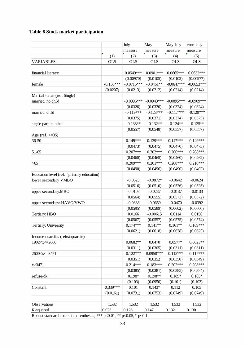
We define a dummy for stock market participation that equals 1 if the respondents hold
investments in stocks and/or mutual funds and 0 otherwise. There is a strong negative
correlation between gender and stock market participation: 33.9% of men in our sample own
stocks, compared with 20.3% of women, a difference of about 14 percentage points (Table 6;
column 1). If we control for the usual background characteristics and the traditional financial
literacy measure (May), we find a strong positive effect of financial literacy on stock market
participation, while the gender effect becomes much smaller but is still significant (column 3).
Compared to men, women have a lower chance (by 4.61 percentage points) to own stocks after
controlling for the usual background information including income, education, and financial
literacy etc. Most importantly, an increase in the level of financial literacy by one standard
deviation results in an increase in the probability to own stocks by 9.01 percentage points. This
result is comparable to the effects found in the literature. While this is a sizeable effect, this
coefficient may reflect confidence as well as knowledge. Next, we run a regression using the
financial literacy measure from the July survey, which is a measure of knowledge and is not
confounded by confidence (column 2). While still significant, the estimate of the effect of
financial literacy goes from 0.0901 to 0.0549, a much smaller effect. Notably, the estimate for
the female dummies becomes more negative compared to the effect on column 3. This is likely
to pick up part of the confidence effect; because women are less confident, they are less likely
to invest in stocks. The July measure for financial literacy is plagued by measurement error
(due to guessing by respondents who are forced to provide an answer). As a result, the estimates
of the effect of financial literacy may be biased towards zero. Indeed, once we use the corrected
May-July measure, the estimate for financial literacy is somewhat higher (column 4). The
difference with the estimate for the July financial literacy measure in column 2 is statistically
significant.
7. Extensions
7.1 Robustness
In our regressions so far, we have included the basic demographic background variables that
are typically included in regressions explaining stock market participation. A possible criticism
is that a number of potentially important explanatory variables are missing. Arguably,
heterogeneity in risk aversion may explain an important part of the variation in stock market
participation. Similarly, individuals display large differences in patience and ability to sacrifice
17
current for future consumption. Moreover, wealthier individuals are more likely to invest in
stocks. The richness of the annual DHS-modules enables us to include household wealth and
variables measuring risk and time preferences. However, there is a cost in terms of a loss of
observations as a result of merging our sample with the survey modules containing information
on the variables mentioned above.
The DHS contains a number of questions in the psychological concepts module that may serve
as a proxy for risk aversion. Respondents are asked to indicate to what extent they agree or
disagree on a number of statements using a scale from 1 to 7, where 1 indicates ‘totally disagree’
and 7 indicates ‘totally agree.’ In Table 7, we use the responses to the statements ‘I am prepared
to take the risk to lose money, when there is also a chance to gain money’ (the variable
spaar6).13 While this type of questions has been used regularly in regressions on stock market
investments (e.g. Kapteyn and Teppa, 2011), one may argue that these are endogenous to stock
market participation. However, our main objective is to investigate whether the estimates of the
effects of financial literacy are sensitive to the inclusion of risk aversion. Note that we do lose
some observations when we incorporate these variables in our regressions in Table 7. We
followed the following strategy: we first merge our dataset with the 2012 psychological
questionnaire which is filled in in the same year as the May and July financial literacy survey.
Next, in order to gain observations we replaced missing values in the spaar1-6 variables with
answers from the two adjacent waves (the 2011 wave and the 2013 wave). We end up with
1,449 observations and loose a limited amount of observations (83).14 Due to the low number
of observations in the two top categories (6 and 7), we merge these respondents together with
the respondents choosing the next highest category 5.
Table 7 shows that the estimates of the financial literacy coefficients are quite similar, albeit
somewhat smaller, and show qualitatively the same patterns among the different financial
literacy measures. However, in comparison with previous estimates, we now have smaller and
insignificant estimates for the gender effect. It seems that the gender effect is explained by risk
13 We performed similar robustness tests using the responses to the statements ‘I think it is more
important to have safe investments and guaranteed returns, than to take a risk to have a chance to get
the highest possible returns’ (the variable spaar1 in DHS) and ‘I do not invest in shares, because I find
it too risky’ (the variable spaar2). The conclusions are similar for stock market participation with the
most important difference that the gender coefficient is somewhat more negative and mostly significant
once we include spaar1 in the stock market participation regression. 14 This is partly due to the restriction that only respondents with net household income in excess of
10000 euro are given these questions.
18
aversion. While insignificant, the pattern is the same as before. The results also indicate that
less risk averse people have a higher tendency to invest in the stock market. In Table 8, we
include measures of time preferences. The estimates of the effects of financial literacy are not
much affected by this variable and the coefficient estimate for the gender dummy also remains
negative and statistically significant.
Apart from including risk and time preferences, we run additional robustness tests. For example
we include numeracy as a proxy for ability (which could be an omitted variable), and we took
into account who is the financial decision-maker in the household. While adding these variables
do help explaining the heterogeneity in stock market participation, they do not affect our main
findings.
7.2 Instruments for financial literacy
Does financial knowledge affect participation in the stock market or is the participation in the
stock market that increases financial knowledge? For example, investors are likely to gather
information before they buy or sell stocks and mutual funds and will more closely follow the
stock market than non-investors. Thus, one cannot give a causal interpretation to the positive
estimates of the financial literacy coefficient in the OLS regressions we have reported so far.
Below, we report the results of regressions based on GMM estimates. Like in previous work,
we use financial education in high school as instruments for financial literacy to identify the
causal effect of financial literacy on stock market participation and to reduce measurement error
in the literacy variable (van Rooij et al. (2011)). Our instruments are based upon information
on exposure to economic education when young, thus before respondents invested in the stock
market.
We measure exposure to education before entering the job market using the responses to the
questions ‘How much of your education in high school was devoted to economic subjects?’
with the following answer categories: ‘a lot’, ‘some’, ‘little’, ‘hardly at all’, ‘not applicable, I
did not complete high school’, ‘do not know’ or ‘refuse to answer’. We distinguish three groups.
The first group consists of respondents who did not get economics in high school answering
‘hardly at all’ or ‘not applicable’. This is the reference group in our empirical analysis. Second,
based on the ‘a lot’, ‘some’ and ‘little’ responses we create a dummy variable for respondents
who were exposed to economics during high school. The third group consists of those who
answered with ‘don’t know’ or ‘refusal’ (very few respondents refused to answer this question).
19
These two groups have high predictive power for financial literacy as shown by the F-values in
the first stage regression which are mostly above 10 (columns 2, 4, 6 and 8 in Tables 9).
Unless respondents indicate they did not complete high school, they receive the next follow-up
question: ‘Did you have at least one economics subject in your final examination year?’ with
the response options ‘yes’, ‘no’, ‘not applicable, I didn’t do a final exam’, ‘do not know’ or
‘refuse to answer’. We create an additional instrument dummy variable that takes the value 1
for those respondents who answer ‘yes’ and the value 0 otherwise. Inclusion of this variable
increases the F-value of the first stage regression to well above 10 for most regressions
(columns 1, 3, 5 and 7 in Tables 9). One may argue, however, that the third instrument dummy
is not valid as for some students the economic subject in their final exam may have been a
choice variable and thus is likely to be correlated with interest in financial matters (interest in
financial matters is an omitted variable in our regression) which in turn may affect financial
decision making. Therefore, we present the results including and excluding this variable in set
of instruments for financial literacy.
Tables 9 presents the GMM results for stock market participation. Both sets of instruments
predict the endogenous financial literacy variable reasonably well. We obtain F-values close to
10 for the July measure and in excess of 10 (which serves as the recommended threshold value
to avoid weak instruments problems in the literature, see Staiger and Stock (1997) for the other
measure). We interpret this as another sign that the July measure contains considerable
measurement error, which makes it more difficult to find good instruments. The Hansen J test
results indicate that the overidentifying restrictions cannot be rejected in any of the
specifications. The GMM C tests (see Hayashi, 2000) show mixed results for stock market
participation. Using the extended set of instruments, the test suggests that financial literacy is
endogenous to stock market participation, while using the smaller set of instruments it cannot
be rejected that financial literacy is exogenous. The latter result is consistent with previous
findings (Van Rooij et al., 2011).
Focusing on the effect of financial literacy on stock market participation, we find that the GMM
estimate of the literacy coefficient is statistically significant at the 5 percent level and relatively
similar across specifications (around 0.20). This seems a comforting result as the instruments
seem to take care of the measurement error problem and the differences between the literacy
measures become less important when good instruments are available. However, finding good
20
instruments is easier for more accurate measures. Note that the predictive value of the
instruments is lowest for the July measure, which translates into a less precise estimate for the
GMM financial literacy estimate. Note also that the gender effect is insignificant in all
specifications, which suggests that once financial literacy and socio-demographic variables are
controlled for, females are as likely to invest in stocks as men. However, while being
insignificant, the patterns for gender differences remain unchanged: in the regressions including
the May financial literacy measure (which jointly measures knowledge and confidence), the
impact of the female coefficient is lower than in the other specifications. We have also run the
GMM regressions on the extensions discussed in section 7.2 (for brevity, not reported). The
main conclusions are not affected.
7.3 How to measure financial literacy?
From a survey methodology point of view, our findings show that financial literacy is best
measured by combining the two surveys and taking into consideration confidence in the
answers. In practice, having two surveys among the same group of respondents is not always
feasible or is also less attractive in terms of the budget normally available for research projects.
A possible way out is to combine the two surveys into a single survey. For example, researchers
may first provide the financial literacy question including the DK option. If the respondent
chooses the DK options, the same question is asked again, this time excluding the DK option.
After providing the answer, either the first or the second time, the respondent is asked for his
or her confidence in the answer. The potential disadvantage of this strategy is that, when a
number of financial literacy questions are asked, respondents will learn that they are required
to answer the same question when answering DK. They may consequently avoid the DK option
and answer the literacy questions right away, which takes away the value added of the DK
option for the researcher. Moreover, this methodology does not capture the information that
was retrieved from the inconsistent answers in the two surveys. Another disadvantage of this
approach is that one needs to include three questions in the survey design to learn about the
response on one literacy question, which may be problematic if there are constraints to the
length of the survey in terms of costs or the duration of the survey.
Alternatively, one could base the financial literacy measures solely on the information content
as contained in the second survey. This requires two responses for each financial literacy
question. A disadvantage is that we lose the information relative to inconsistent answering
across surveys. However, the number of inconsistent responses is limited and the DK answers
21
show a strong correlation with the confidence questions (see Table 3). The extent to which our
combined measure based on two surveys is better able to capture true knowledge than a measure
using the questions in the second survey only (both the literacy question plus the confidence
question) is an empirical question. Below, we will investigate the difference between these two
approaches. First, we construct a measure for financial literacy based upon the financial literacy
and confidence questions in survey two only (as discussed in Section 4.2). Basically, we assume
that respondents indicating they are very unsure about their answers are not knowledgeable,
even if they guess the answer correctly. The analysis in Table 4 shows that this measure is
closely related to the measure based on both survey waves. In addition, the regression results
for stock market participation show that the estimate of the effect of financial literacy becomes
somewhat smaller (compare column 5 and 4 in Table 6). This is consistent with the fact that the
measure employing both surveys is better able to filter out guessing and thus has less
measurement error. However, note that the measurement error is much lower than in using the
July financial literacy questions and not the confidence questions (compare column 5 and 2 in
Table 6). The financial literacy coefficients are economically and statistically significantly
higher than for the July measure. Overall the results for the alternative methods of measurement
based on only the July questions plus confidence are quite similar to those based upon the
measure combining both surveys. These findings show that the alternative measure provided in
the July survey may provide an adequate proxy for true knowledge while it is much easier to
integrate in new research designs and with less costs.15
8. Concluding remarks
The literature has documented large and robust gender differences in financial literacy. For
example, Lusardi and Mitchell (2011b) find that 22.5% of female respondents in the US were
able to answer 3 simple questions on inflation, interest and risk diversification correctly versus
38.3% of male respondents. These findings are robust across different surveys and different
countries (Lusardi and Mitchell, 2011a). This is especially worrisome as women tend to outlive
their husband and will have to make financial decisions later in life (Lusardi and Mitchell,
2008).
15 In principle one may consider to include a whole lot of literacy questions as well. The distorting effect
of measurement error due to random guessing is likely to diminish when respondents have to guess
many questions. However, this strategy would most likely require so many questions that it is either not
feasible to implement or very costly in terms of question load.
22
In our work, we find that the gender gap in the measures of financial literacy diminishes a lot
when we take away the option of answering “I do not know (DK)”. The higher propensity that
women display to choose DK is related to a lack of confidence. The gender gap diminishes
significantly once we correct the traditional financial literacy measures to get improved
measures for knowledge, but the gap does not disappear. By and large, we find that only half
of the gender gap in financial literacy can be explained by confidence and other background
variables, such as income and education.
Our findings have implications for both the survey methodology used to measure financial
literacy and for measuring the effects of financial literacy on behavior. Traditional financial
literacy measures are a combination of confidence and financial knowledge. This has
consequences for assessing the effects of both gender and financial literacy in regressions
explaining financial decision-making. When respondents are forced to choose an answer,
financial literacy measures are not contaminated by confidence and are better able to proxy true
knowledge. However, this introduces measurement error as respondents who are not
knowledgeable are forced to guess the correct answer. We propose an adjusted metric to
measure pure knowledge which suffers less from measurement error. This new measure
provides different findings for the effects of financial literacy on financial decisions. In terms
of policy, it is often crucial to disentangle true knowledge from confidence. For example, for
an effective design of initiatives raising financial education and increasing awareness it is
important to figure out whether it is limited knowledge or low confidence that explains low
stock market participation. Using our improved measure, we show that true financial knowledge
contributes to explain a sizeable part of the observed heterogeneity in important household
financial decisions, such as investing in the stock market.
23
References
Agarwal, S., Driscoll, J., Gabaix, X. and Laibson, D. (2009). The age of reason: Financial
decisions over the life cycle and implications for regulation, Brookings Papers on Economic
Activity, Fall 2009, pp. 51-117.
Alessie, R., Van Rooij, M. and Lusardi, A. (2011). Financial literacy and retirement preparation
in the Netherlands, Journal of Pension Economics and Finance, vol. 10(4), pp. 527–546.
Barber, B. and Odean, T. (2001), Boys will be boys: gender, overconfidence and common
stock investment, Quarterly Journal of Economics, February 2001, pp. 261-292.
Beyer, S. (1990), “Gender differences in the accuracy of self-evaluations of performance”,
Journal of Personality and Social Psychology, 59(5), pp. 960-970.
Bucher-Koenen, T., Lusardi, A., Alessie, R. And Van Rooij, M. (2014), How financially
literate are women? An overview and new insights, NBER Working Paper No. 20793.
Chen, Haiyang and Ronald P. Volpe (2002), Gender differences in personal financial literacy
among college students, Financial Services Review, 11, pp. 289-307.
Dahlbom, L., A. Jakobsson, N. Jakobsson, and A. Kotsadam (2011), Gender and
overconfidence: Are girls really overconfident?, Applied Economics Letters, 18, 325-327.
Hayashi, F. (2000), Econometrics. 1st ed. Princeton, NJ: Princeton University Press.
Kapteyn, A., and Teppa F. (2011). Subjective measures of risk aversion, fixed costs, and
portfolio choice, Journal of Economic Psychology, vol. 32(4), pp. 564–580.
Lusardi, Annamaria, and Olivia S. Mitchell (2008). Planning and financial literacy: How do
women fare?, American Economic Review, 98(2), pp. 413-417.
Lusardi, Annamaria and Olivia S. Mitchell (2011a), Financial literacy and planning:
Implications for retirement wellbeing, in Olivia S. Mitchell and Annamaria Lusardi (eds.),
Financial Literacy: Implications for Retirement Security and the Financial Marketplace.
Oxford: Oxford University Press, pp. 17-49.
Lusardi, A. and Mitchell, O. (2011b). Financial literacy around the world: an overview, Journal
of Pension Economics and Finance, vol. 10(4), pp. 497–508.
Lusardi, A. and Mitchell, O. (2011c). Financial literacy and retirement planning in the United
States”, Journal of Pension Economics and Finance, 10(4), pp. 509-525.
Lusardi, A. and Mitchell, O. (2014). The economic importance of Financial Literacy: Theory
and evidence, Journal of Economic Literature, vol. 52(1), pp. 5-44.
Mahdavi, M. and Horton, N. (2014), Financial knowledge among educated women: Room for
improvement, Journal of Consumer Affairs, 48 (2), pp. 403–417.
24
OECD (2013), Women and financial education: Evidence, policy responses and guidance,