Word Problem Combined - McGill University

The word problem for computads

*by M. Makkai

McGill University

(Revised May 16, 2005)

Contents:

Introduction p. 1

1. Concrete presheaf categories p. 20

2. ω-graphs p. 26

3. ω-categories p. 27

4. Adjoining indeterminates p. 32

5. Computads p. 42

6. Multitopes and computopes p. 50

7. Words for computads p. 59

8. Another set of primitive operations for ω-categories p. 66

9. A construction of the one-step extension X[U] p. 75

10. Solution of the word problem p. 88

11. Proof of the existence of enough computopes p. 104

Appendix to section 1 p. 109





References p. 145

* Supported by NSERC Canada

Introduction

(A) The origins of the paper

Computads were introduced by Ross Street, for dimension 2 as early as 1976 in [S1]

and in general, in [S3]. Albert Burroni's paper [Bu] calls computads "polygraphs". Jacques

Penon's paper [Pe] is important for us, since it contains the full syntactical definition of

computads (reproduced with small changes in section 7 below), which will be used to

formulate the problem in the title of the present paper.

My interest in computads stems from their role in the definition and theory of weak

higher-dimensional categories. This role came to be realized as an afterthought.

In [He/M/Po], the definition of "opetopic set" introduced by John Baez and James Dolan

[Bae/D] is reworked into what we called "multitopic set". In [He/M/Po], it was shown, among

other, that the category of multitopic sets is, up to equivalence, the same as the category of

presheaves on a category called the category of multitopes. In [M3], inspired by the second

part of the Baez/Dolan definition of "opetopic category", but also following my earlier work

[M1], [M2] on logic with dependent sorts, I proposed a definition of "the large multitopic

category of all small multitopic categories"; the small multitopic categories constitute the

zero-cells in said large multitopic category.

Already at the time of our joint work with Claudio Hermida and John Power, we had the

feeling that multitopic sets were related to computads, in fact, that they were essentially

identical with the "many-to-one" computads, ones whose indeterminates (free generating cells)

have codomains that are themselves indeterminates (although, I must confess, at the time I did

not really understand the notion of computad). The paper [Ha/M/Z] established this result, in

the form of a pair of adjoint functors between the category of multitopic sets on the one hand,

and the category of small ω-categories on the other, under which the left adjoint functor, from

the first of the above categories to the second, being faithful and full on isomorphisms, has, as

its essential and full-on-isomorphisms image, the category of many-to-one computads.

This result represented an advance inasmuch the fairly complicated, albeit combinatorially

explicit, original definition in [He/M/Po] of multitopic sets became a conceptually simple one.

On the other hand, it is to be noted that the fact that the category of many-to-one computads is

a presheaf category, and the implied equivalent concept to the notion of multitope, do not

1

become obvious by merely looking at many-to-one computads. At the present stage of our

knowledge, said fact needs, for its proof, the detour via the original theory of multitopic sets in

[He/M/Po].

The basic perspective of the present paper is a reversal of the above chronology. The notions

"multitopic set" and "multitope" are seen here as the result of a combinatorial/algebraic

analysis of the notion of many-to-one computad. The paper attempts to extend said analysis to

all computads.

(B) Computads as the algebraic notion of higher–dimensional diagram.

The notion of computad is, as far as I am concerned, nothing but the precise notion of

higher-dimensional categorical diagram. To explain this, I start earlier, with an informal

introduction to the notion of (strict!) ω-category. (In this paper, no "weak" category theory

appears at all.)

Consider the following ordinary categorical diagram:

f f3 6X A��@X A��@X3 6 9O O O� � �g � 2 g � 4 �g2� 4� � 6

X A��@X A��@X2 f 5 f 82 5O O Og � g � �g1� 1 3� 3 � 5� � �X A��@X A��@X1 f 4 f 71 4

consisting of objects X and arrows f , g in some category. The reader will agreei j kwhen we say this:

(*) if the four small squares 1, 2, 3, 4 commute,

then, as a consequence, the big outside square will commute as well.

Having agreed on this, one may ask what are the general laws behind this, and countless other

similar and/or more complicated facts. The answer is: the laws codified in the definition of

2

notion of " ω-category".

To motivate that definition, the starting point is to adopt the position that "there is no bare

equality": every equality is mediated by some data that we -- conveniently or not -- forget

when we simply assert the fact of an equality. (At the Minneapolis (IMA) meeting on

higher-dimensional categories in June 2004, John Baez gave, as the introductory talk to the

conference, a brilliant lecture with this theme.) That position dictates that we, abstractly and

theoretically, introduce data that are responsible for the commutativity of the four numbered

squares above, in the way of fillers, 2-dimensional cells, or 2-arrows, as follows:

f f3 6X A��@X A��@X3 6 9O O O� k � k �g � a g � a �g2� 2 4� 4 � 6

X A��@X A��@X2 f 5 f 8 (1)2 5O O Og � k g � k �g1� a 3� a � 5� 1 � 3 �X A��@X A��@X1 f 4 f 71 4

We think e.g. of a as a (2-)arrow with domain g f , and codomain f g . (We use2 2 3 2 4"geometric order"; g f is what usually is denoted by f vg , or also g #f .) We even2 3 3 2 2 3have given up the symmetry in the idea of the equality g f = f g , and think of g f2 3 2 4 2 3being transformed into f g in some general way, that way being denoted by a .2 4 2

A 2-arrow must have a domain and a codomain that are ordinary ( 1-) arrows, which are

parallel: they share their domain and their codomain, which are 0-cells. The idea here is that a

2-arrow as a transformation does not have any effect on 0-cells: it must leave them alone;

transforming 0-cells is the responsibility of 1-cells.

The "if-then" statement (*) above becomes an operation that, applied to the four arguments

a , a , a , a results in a transformation, say b , of g g f f into f f g g :1 2 3 4 1 2 3 6 1 4 5 6

b: g g f f A��@ f f g g (2)1 2 3 6 1 4 5 6

depicted as

3

f f3 6X A��@X A��@X3 6 9O O� �g � �g2� � 6X X2 b k 8O Og � �g1� � 5� �X A��@X A��@X .1 f 4 f 71 4

The above procedure of introducing 2-dimensional arrows into diagrams to represent

evidence, or proof, of a commutativity is closely related to the similar procedures in proof

theory, especially categorical proof theory; see for example [L/Sc], section I.1, "Propositional

calculus as a deductive system".

The concept of ω-category (" ω- " here anticipates the need for passing to ever higher

dimensions after 0, 1 and 2 that have appeared so far) will have, on the one hand, some

algebraically codified primitive operations that let us obtain b out of a , a , a , a by1 2 3 4repeatedly applying those operations, and on the other, certain laws that ensure that no matter

in what order we apply the primitive operations to the four arguments, the result is always the

same: b is well-defined as the composite of a , a , a , a without any further1 2 3 4qualification.

Just as the commutativity of 1-dimensional diagrams, that is, the equality of composite

1-arrows, has "given rise" to 2-dimensional diagrams, the contemplation of the equality of

composite 2-cells (possible 2-commutativities) gives rise to 3-arrows, and 3-dimensional

diagrams. For instance, the fact that the composite of a , a , a , a equals b is mediated1 2 3 4by a 3-cell

f f f f3 6 3 6X A��@X A��@X X A��@X A��@X3 6 9 3 6 9O O O O O� k � k � � �g � a g � a �g g � �g2� 2 4� 4 � 6 2� � 6X A��@X A��@X Φ X X2 f 5 f 8 �� 2 b k 8 (3)2 5O O O O Og � k g � k �g g � �g1� a 3� a � 5 1� � 5� 1 � 3 � � �X A��@X A��@X X A��@X A��@X1 f 4 f 7 1 f 4 f 71 4 1 4

4

Of course, the process does not stop at dimension 3 , and we see the need for a concept of

ω-category in which there are arrows (cells) of arbitrary non-negative integer dimensions (but

none of dimension ω or ∞ ).

Since the examples like the ones we considered clearly encompass a large variety, especially

when one contemplates arbitrarily high dimensions, it is a highly non-obvious fact that a

satisfactory concept of ω-category is possible at all. It is not a priori clear that there is a neatly

defined set of primitive operations whose combinations account for all the desired

compositions of cells; and it is not a priori clear that there is a neat set of laws that ensure

facts like the one above of b being well-defined as the composite of a , a , a , a . It is1 2 3 4therefore a kind of miracle that in fact we do have a good notion of ω-category. It is the basic

general aim of the present paper and its projected sequels to investigate the ways and means of

this "miracle".

There is another, perhaps even more convincing, way of approaching the concept of

ω-category. This argues that the totality of (small) n-(dimensional) categories, properly

construed, is an (n+1)-category; therefore, if we want to freely form "arbitrary totalities", we

need n-categories for all n . (Let me note that the process stops at ω : the totality of (small)

ω-categories is, in a natural way, an ω-category again, not an (ω+1)-category.) However, in

this second argumentation, when carried out with proper care, we find a similar step of

replacing an equality by a transformation. In fact, this latter thinking, when followed to its

logical conclusion, gives rise to the notion of weak ω-category, a concept that we do not

discuss in this paper. The present paper sticks to the formal or syntactical role of higher

dimensional diagrams, and it does not need the consideration of "totalities".

In an ω-category in which the diagram (3) lives, there are many cells (infinitely many if we

consider the identities of all dimensions required by the concept of ω-category). In particular,

we have the composite 1-cell g f "on the same level" as the generating arrows g ,2 3 2f , etc. The concept that makes the distinction between "generating cell" and "composite3cell" is the concept of computad. This is a conceptually very simple notion; it can be stated as

levelwise free ω-category.

Imagine a structure, a typical computad, that can be taken to be essentially identical with the

diagram (3). We want the elements of this structure to be exactly the named items in the

diagram: the 0-cells X (i=1, ..., 9), the 1-cells f (j=1, ..., 6) , g (k=1, ..., 6),i j k

5

the 2-cells a (l=l, ..., 4), b , and the 3-cell Φ . However, to account for the structurelitself, we need to consider various composites of the elements. We decide to form the

composites freely.

1To begin with, we take the free category X on the ordinary graph consisting of said 0-cells

and 1-cells. To incorporate the 2-cells and their composites, we need the operation of freely

1adjoining the mentioned 2-cells as indeterminates to X , with the appropriate preassigned

1domains and codomains given as certain (composite) 1-cells in the category X .

This process of free adjunction is very familiar from algebra. The ring of polynomials

R[X, Y, ...] is obtained from the ring R , by freely adjoining the indeterminates

X, Y, ... . The definition, via a universal property, is too familiar to be quoted here. The

2 12-category X obtained by the free adjunction of the appropriate 2-cells to X , with the

1specified domains and codomains in X , is defined by a similar universal property. The only

additional complication is that the adjoined 2-cell a , to have an example, is constrained to21have the specified domain g f and codomain f g given in X already. In the section2 3 2 4

I.5, "Polynomial categories", of [L/Sc], we find a similar situation in which an arrow with

preassigned domain and codomain is freely adjoined to Cartesian closed category. (The

definition of computad is given in section 5 , based on section 4.)

When we adjoin an indeterminate u to an ω-category X in which we have specified du

and cu in X , to get X[u] , we usually assume that du and cu are parallel: they have

the same domain and codomain. However, this is only a "reasonability assumption". The

definition through the appropriate universal property works without this assumption. The

canonical map F:XA@X[u] will naturally produce the equality

F(ddu)=F(dcu)=d (u) . Thus, F can be injective only if said parallelism conditionX[u]is satisfied. As we will see, in that case, F is indeed injective. � 2The composite of a , a , a , a will be a definite 2-arrow a in X . Of course, this is a1 2 3 4major point of the construction, and it has to be ascertained specifically. That is, we have to

define, using the primitive operations of " ω-category", a specific 2-cell that we will take, by

definition, to be the composite of a , a , a , a . This we will not do here, since we do not1 2 3 4have the formalism of ω-category yet. However, once we have done this, the resulting 2-cell

6

� �a will have domain and codomain as b does in (2); in other words, a will be parallel to

b .

Finally, the whole structure -- a computad -- is obtained by freely adjoining the 3-dimensional

2 �indeterminate Φ to X , with the stipulation that d(Φ) is to be the composite a , and

c(Φ) is b .

We have outlined the definition of a particular ω-category, in fact, a computad, that we take

to be the structure representing the pasting diagram (3). It gives a good idea of the general

notion of computad.

It turns out (see sections 4 and 5) that, when we define a computad to be an ω-category

without additional data as we did in the example, we are able to recover the indeterminates in

the computad from its ω-category structure as the elements that are indecomposable in a

natural sense. Thus, it is not necessary to carry the indeterminates as data for the structure.

I consider the notion of computad as being identical to the notion of higher dimensional

diagram, or pasting diagrams.

An analysis, using combinatorial, algebraic or geometric means, may provide descriptions

amounting to equivalent definitions of smaller or larger classes of computads. In fact, such

descriptions are one of the main areas of the theory of computads. As I mentioned above, the

paper [Ha/M/Z] is part of this area.

The notion of a diagram being pastable (composable), the focus of the attention in the theory

of pasting diagrams, is implicit in the concept of computad, since a computad always carries

within itself all possible (free) compositions of the indeterminates (elements of the diagram).

Of course, this does not mean that the problem of pastability of given candidates of pasting

diagrams, given in some combinatorial or other manner, is solved automatically by using

computads. The value of computads is mainly in their ability to provide mathematically

satisfactory definitions of intuitive concepts -- such as pastability --, which then can be

analyzed in any manner that comes to mind.

The important papers [J], [Po1], [Po2], [Ste]) give with various combinatorial, algebraic and

geometric definitions of classes of pasting diagrams. They make connections to computads to

7

varying degrees. In ongoing and future work (e.g. [M4]), I revisit the results of the existing

theory of pasting diagrams in the spirit of computads.

(C) Concrete presheaf categories.

In part (A) above, we mentioned two results, both asserting the equivalence of certain

categories. The first said that MltSet , the category of multitopic sets, is equivalent of

op MltMlt = Set , with Mlt the category of multitopes. The second said that MltSet

is equivalent to Comp , the category of many-to-one computads.m/1

It turns out that in both cases, what is proved is stronger than what is stated. In both cases, we

have equivalences of concrete categories.

A concrete category is a category A together with an "underlying-set" functorQ-R:AA@Set . Equivalence of concrete categories (A, Q-R ) , (B, Q-R ) is equivalenceA Bof categories compatibly with the underlying-set functors: we require the existence of a functor

Φ:AA@B that is an equivalence of categories, such that the following diagram of functors:

ΦAG��@B�� t�� ≅ ��h WQ-R Set Q-RA B

≅commutes up to an isomorphism: there is an isomorphism ϕ:Q-R A��@Q-R vΦ .A BAll three of the above-mentioned categories MltSet , Mlt , Comp are equippedm/1with canonical underlying-set functors.

A multitopic set, an object of MltSet , consists of n-cells, for each n∈ � ; we have an a

priori underlying-set functor Q-R:MltSetA�@Set . ( In the notation of [He/M/Po] , Part 3,

p. 83, for the multitopic set S , QSR= $ C ; the elements of C are called the k-cells ofk kk∈ �S . In [Ha/M/Z], §1 gives an alternative, possibly more conceptual introduction to multitopic

sets. On p.51 loc.cit., it is pointed out that in dimension 0 , a detail in the definition in

[He/M/Po] is to be corrected.)

8

op CFor any small category C , we take the presheaf category C=Set to be equipped withthe underlying-set functor Q-R:CA@Set defined as QAR= $ A(U) .U∈ Ob(C)

We have the underlying-set functor Q-R:CompA@Set which assigns to each computad X

the set QXR of all indeterminates of X . Comp is a concrete category with them/1underlying-set functor the restriction of that for Comp .

It turns out that both equivalencesMltSet J MltComp J MltSetm/1

are in fact concrete, that is, compatible with said underlying-set functors. As a corollary, we

have the concrete equivalence Comp J Mlt .m/1

This statement is meaningful even if we do not know the precise definition of Mlt ; it says

that Comp is (concrete-equivalent to) a concrete presheaf category.m/1

A concrete presheaf category is, of course, in particular, a presheaf category; thus it is a very

"good" category. Let us see what the "concreteness" in the equivalence says, in addition.The concrete equivalence of (A,Q-R) and C means that we have an equivalence functorJ F:AA�@C , and a natural bijectionQAR ≅ $ (FA)(U) . (A∈ A) .U∈ Ob(C)

Thus, up to a natural bijection, we have a classification of the elements of an object A (the

elements of the set QAR ) of A into mutually disjoint classes (FA)(U) , the classes being

labelled with a fixed set of types, the objects U of C . This classification is functorial: it is

compatible with the arrows of A . Moreover, we have arrows between the types, the

9

ftype-arrows, that account for the complete structure of the category A : an arrow AA��@B ,

essentially a natural transformation, is given by a system of maps

fU(FA)(U)A��@(FB)(U) , one for each type U , that are jointly compatible with the

type-arrows. It turns out that the equivalence type a concrete presheaf category C determines C up to

isomorphism; we say that C is the shape category of any concrete category that is concretelyequivalent to C .

*Given a concrete category A=(A, Q-R) , we identify a category, denoted by C [A] , which

is the shape category of A in case A turns out to be a concrete presheaf category. Here is the

definition.

El(A) denotes the category of elements of the functor Q-R:AA@Set ; its objects are pairs

(A, a) = (A∈ A, a∈ QAR) , and they are called elements of A .

An element (A, a) is said to be principal if it is A is generated by a , in the sense that

whenever f:(B, b)A@(A, a) is an arrow in El(A) such that f:AA@B is a

monomorphism in A , then f is an isomorphism. The element (A, a) is primitive if it is

principal, and for any principal (B, b) , any arrow f:(B, b)A@(A, a) must be an

isomorphism.

*The shape category C [A] has objects that are in a bijective correspondence with the

isomorphism types of primitive elements (A, a) . Moreover, if the primitive elements

*(A, a) , (B, b) are (represent) objects of C [A] , then an arrow (A, a)A@(B, b) in

*C [A] is the same as an arrow AA@B in the category A . Thus, there is a full and faithful

*forgetful functor C [A]A@A .

Furthermore, we can spell out a set of conditions, some of them involving the primitive

elements of A , that are jointly necessary and sufficient for A to be a concrete presheaf

category.

The first group, (i), of the conditions says that A is small cocomplete, Q-R:AA@Set10

preserves small colimits, and reflects isomorphisms.

The second group contains four conditions.

The first, (ii)(a), says that the set of isomorphism types of primitive elements is (indexed by a)

small (set).

The second, (ii)(b), says that every element is the specialization of a primitive element:

for every element (A, a) of A , there is a primitive element (U, u) together with a

map f:(U, u)A�@(A, a) in El(A) .

Here, (U, u) is said to be a type for (A, a) , f a specializing map for (A, a) .

The third condition, (ii)(c), says that, for any element (A, a) , with any given primitive

(U, u) , there is at most one specializing map (U, u)A@(A, a) .

Finally, the last one, (ii)(d), says that if the primitive elements (U, u) , (V, v) are both

types for (A, a) , then they are isomorphic: (U, u)≅ (V, v) .

All the above facts concerning concrete presheaf categories are established as parts of standard

category theory; they are easy, but form a basic setting for the first of the two main lines of

inquiry in the paper, the investigation of the category Comp and certain of its full

subcategories as to which of the above conditions are satisfied in them. Comp is one ofm/1those full subcategories, and, by what we know from previous work, it satisfies every one of

said conditions.

It is relatively easy to show that Comp itself satisfies (i) and (ii)(a); see the work leading up

to section 6. One of the main results of the paper that Comp satisfies (ii)(b) ; every element of

Comp has at least one type. The proof of this result requires the more substantial tools of the

paper developed in sections 8 , 9 and 11. An easy example shows that (ii)(c) fails in Comp

(see section 6). I do not know if (ii)(d) is satisfied or not by Comp .

Let C be a sieve in Comp , that is a full subcategory of Comp for which if B is in C , and

AA@B is any arrow, then A is in C . ( Comp is an example for a sieve in Comp ). Cm/1is regarded as a concrete category with the underlying-set functor inherited from Comp . It is

11

then immediate that the notions of principal element, primitive element, and type for an

element for C become the direct restrictions of those for Comp . More precisely, for (A, a)

in El(C) , (A, a) is principal resp. primitive for the concrete category C just in case it is

principal resp. primitive for Comp . Moreover, obviously, for an element (A, a) of C , any

(U, u) is a type of (A, a) in the sense of the concrete category Comp if and only if

(U, u) is a type of (A, a) in the context of the concrete category C .

Thus, for a sieve C in Comp , to say that it is a concrete presheaf category, is to say that it

satisfies (i) -- which is ensured by assuming that C is closed under colimits in Comp --, and

that the conditions (ii)(c) and (ii)(d) are satisfied by primitive elements of Comp that belong

to C .

An additional simplification is provided by the fact that a principal element (A, a) of Comp

is determined by the underlying computad A ; a is the unique indeterminate of maximal

dimension in A ; it is denoted by m . We call A a computope if (A, m ) is primitive. IfA AC is a sieve in Comp , and as a concrete category is a concrete presheaf category, then its

*shape category C [C] is the skeletal category of the computopes that are in C .

Furthermore, it is a one-way category (all non-identity arrows AA@B have

dim(A)<dim(B) ), which makes it amenable to the manipulations of logic with dependent

sorts ([M1], [M2]).

In particular, multitopes can be identified with many-to-one computopes: an elegant, albeit

fairly abstract, definition of "multitope".

Here is an example illustrating the role of computopes.

Consider the diagram

fhf h A��@A��@ A��@ �X Y Z ; X a� Z . (4)A��@ A��@ Pg i A�� @gi

(recall the use of geometric order in compositions). It is clear how to interpret (4) as a

computad: once again, the elements (indeterminates) of the computad are exactly the distinct

elements named by single letters in the figure. (4) is a principal computad; its main cell

( m ) is a .(4)

12

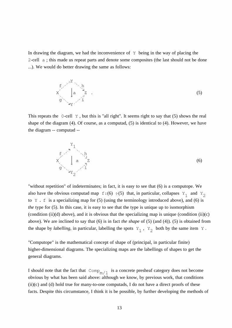
In drawing the diagram, we had the inconvenience of Y being in the way of placing the

2-cell a ; this made us repeat parts and denote some composites (the last should not be done

...). We would do better drawing the same as follows:)YK� f� h� k�X a Z . (5) P ) �g � ik HYThis repeats the 0-cell Y , but this is "all right". It seems right to say that (5) shows the real

shape of the diagram (4). Of course, as a computad, (5) is identical to (4). However, we have

the diagram -- computad --

Y1) K� f� h� k�X a Z (6) P ) �g � ik HY2

"without repetition" of indeterminates; in fact, it is easy to see that (6) is a computope. We

also have the obvious computad map f:(6)A@(5) that, in particular, collapses Y and Y1 2to Y . f is a specializing map for (5) (using the terminology introduced above), and (6) is

the type for (5). In this case, it is easy to see that the type is unique up to isomorphism

(condition (ii)(d) above), and it is obvious that the specializing map is unique (condition (ii)(c)

above). We are inclined to say that (6) is in fact the shape of (5) (and (4)). (5) is obtained from

the shape by labelling, in particular, labelling the spots Y , Y both by the same item Y .1 2

"Computope" is the mathematical concept of shape of (principal, in particular finite)

higher-dimensional diagrams. The specializing maps are the labellings of shapes to get the

general diagrams.

I should note that the fact that Comp is a concrete presheaf category does not becomem/1obvious by what has been said above: although we know, by previous work, that conditions

(ii)(c) and (d) hold true for many-to-one computads, I do not have a direct proofs of these

facts. Despite this circumstance, I think it is be possible, by further developing the methods of

13

this paper, to show that further significant categories of computads are concrete presheaf

categories.

Perhaps it is not superfluous to state that my interest in higher-dimensional diagrams, hence, in

computads in general, stems from the view that they should constitute the language for talking

in a flexible way about matters within weak higher dimensional categories. Although the

many-to-one computads are sufficient for defining a suitable concept of higher-dimensional

weak category, a flexible language to develop mathematics in the context of a suitable weak

higher-dimensional category, in analogy to mathematics developed in a topos, one needs

higher-dimensional diagrams in general.

(D) The word problem for computads

For a fully explicit, computationally adequate, implementation of higher-dimensional diagrams

-- that is, computads -- we need a notational system to represent, not only the indeterminates,

but also the pasting diagrams, or pd's, i.e., all composite cells, in the computad. After all, we

must input the information about the domain and the codomain (arbitrary pd's in general) of

each indeterminate.

The formalism of ω-categories provides such a notational system; as usual with free

constructions, we can denote all cells of the ω-category freely generated by indeterminates by

using a system of words derived directly from said formalism. This method is familiar from

algebra, for instance, in the study of free groups, or more generally, groups given by

presentations. In the case of computads, there is a new element, namely, the necessity to

consider the condition of a word being well-formed. This becomes clear on the conditional

nature of composition: one needs the precondition that a domain be equal to a codomain for

the composite to be well-formed. However, having realized that we have to talk about

well-formedness, the system of words is naturally defined. In this paper, this is done in section

7, following Jacques Penon's system in [Pe].

Similarly to what happens in the algebra of groups, the pd's in a computad will be identified

with equivalence classes of words, rather than with words simply; the laws of ω-category will

make certain pairs of words equivalent, that is, denote the same pd in the computad. The

question how to see if two words are equivalent naturally arises, and one wants to know if the

word problem is solvable: whether or not there is an decision method, efficient if possible, to

14

decide for any two words if they are equivalent. Only in possession of such a decision method

can we hope to have a reasonably general way of handling higher-dimensional diagrams

computationally.

One of the main results of this paper is that the word problem for computads in general is

solvable. After preparations, the main part of the work of the proof is done in section 10.

The motivation for this result also came from the situation of the many-to-one computads. In

[Ha/M/Z] and independently, in [Pa], there is a description of the ω-category, in fact, a

typical many-to-one computad, generated by a multitopic set, in which the general cells of the

ω-category are given as multitopic pd's of the multitopic set "with niches". (In [Ha/M/Z], this

is given as the left-adjoint of a pair of adjoint functors between MltSet and ωCat , the

right adjoint of which is a multitopic nerve functor). The construction provides a normal form

for words denoting the pd's of the many-to-one computad. Starting from any many-to-one

word, its normal form is computable, and two words are equivalent iff their normal forms are

identical; the word problem of many-to-one computads is solvable as a consequence.

The solution of the word problem for general computads starts in a similar manner, with

reducing an arbitrary well-formed word to a "pre"-normal form. The question of equivalence of

pre-normal words is still non-trivial, but it is simpler than that for raw words, and it is

eventually manageable, although the decision procedure as it stands at present uses searches

through fairly large finite sets, and therefore it is quite unfeasible.

(E) The contents and the methods of the paper

The paper separates into two parts, one that uses, and the other that does not use, words.

Sections 7 and 10 use, and are about, words. The other sections do not mention words, or use

results based on words, at all.

The elementary theory of equivalence to a concrete presheaf category is explained in section 1.

Here, and elsewhere, the proofs that were found boring or less than easily readable were put

into appendices. On the other hand, the paper, taken as a whole, is more than usually

self-contained.

15

Sections 2 and 3 contain the generally accepted definitions of ω-graph and ω-category.

Compare [Str2].

Sections 4 and 5 contain the concepts underlying the definition of "computad", and the basic

results concerning these concepts. The approach is leisurely and the proofs are mostly routine.

Section 4 explores the operation of adjoining indeterminates to a general ω-category, and the

iteration of this operation. Section 5 defines computad as an ω-category obtained by iterated

adjunctions of indeterminates to the empty ω-category. The emphasis in section 5 is on the

properties of the category Comp of all computads, and the way this category resembles

"good" categories such as presheaf categories.

The one element of section 5 that seems to be novel is the concept of the content of a pd in a

computad: this is a multiset of the indeterminates occurring in the pd, counting the multiplicity

(number of occurrences) of each indeterminate.

The definition of the content function was a non-trivial matter, and in fact, it is not entirely

successful. One of the main intuitive requirements would be that in case of a computope A ,

the multiplicity of each occurring indeterminate in m is equal to 1 . Our definition of theAcontent function definitely does not satisfy this; and I do not know if it is possible to give such

a definition, also having the other desired properties.

Despite its drawbacks, the content function is an efficient tool for the main purposes of the

paper. One needed property is its invariance under equivalence. Its verbal description sounds

as if it is defined for words, by a direct count of occurrences. However, such a definition

would not give something that is invariant under equivalence of word, that is well-defined for

pd's. As a matter of fact, the definition of the content is not done using words at all.

Another crucial property of "content" is its "linear" behaviour under maps of computads; see

5.(12)(ix).

Section 6 was fairly completely described under (C).

Section 7 displays the system of words for computads in complete (and straight-forward)

detail.

Sections 8 and 9 contain the main mathematical novelty in the paper. I propose a kind of

normal form, the expanded form, for compound expressions (words) in the language of

16

ω-categories. The expanded form is constrained in two ways. The first is that it admits only

restricted instances of the ω-category operations. Specifically, the operation a# b is allowedkfor cells a of dimension m and b of dimension n only if k=min(m, n)-1 . Since k is

determined by a and b , its notation is not necessary; we write a ⋅b for a# b .k

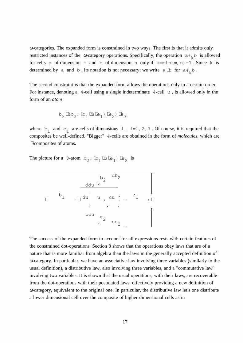
The second constraint is that the expanded form allows the operations only in a certain order.

For instance, denoting a 4-cell using a single indeterminate 4-cell u , is allowed only in the

form of an atom

b ⋅(b .(b ⋅u ⋅e ) ⋅e ) ⋅e3 2 1 1 2 3

where b and e are cells of dimensions i , i=1, 2, 3 . Of course, it is required that thei icomposites be well-defined. "Bigger" 4-cells are obtained in the form of molecules, which are

⋅ -composites of atoms.

The picture for a 3-atom b .(b ⋅u ⋅e ) ⋅e is2 1 1 2�� db �� b 2 �� 2 �� P �� ddu �� A�� Pb � � � P e1 du� u �cu 1⋅A��@ ⋅ �A��@� .A��@ ⋅� �� P P� � O� � � O� A�� ccu �� e �� 2� P ce �� 2 �A��The success of the expanded form to account for all expressions rests with certain features of

the constrained dot-operations. Section 8 shows that the operations obey laws that are of a

nature that is more familiar from algebra than the laws in the generally accepted definition of

ω-category. In particular, we have an associative law involving three variables (similarly to the

usual definition), a distributive law, also involving three variables, and a "commutative law"

involving two variables. It is shown that the usual operations, with their laws, are recoverable

from the dot-operations with their postulated laws, effectively providing a new definition of

ω-category, equivalent to the original one. In particular, the distributive law let's one distribute

a lower dimensional cell over the composite of higher-dimensional cells as in

17

a ⋅(b ⋅e) = (a ⋅b) ⋅(a ⋅e) ,

where dim(a)<dim(b) , dim(a)<dim(e) , and the expressions are well-defined. It is

mainly this that allows to reduce an arbitrary word to the form of a molecule.

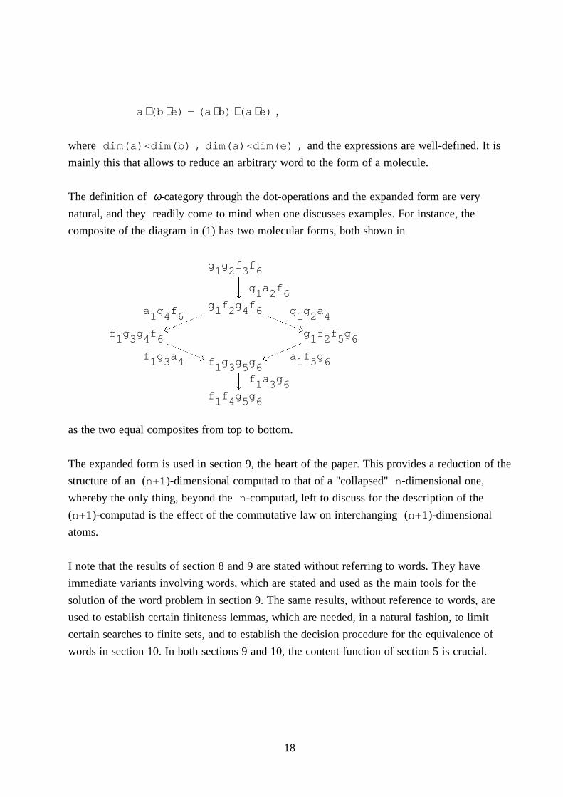
The definition of ω-category through the dot-operations and the expanded form are very

natural, and they readily come to mind when one discusses examples. For instance, the

composite of the diagram in (1) has two molecular forms, both shown in

g g f f1 2 3 6�� g a fP 1 2 6g f g fa g f 1 2 4 6G g g a1 4 6��t �� 1 2 4�� W hf g g f g f f g1 3 4 6G 1 2 5 6�� t�� f g a h W a f g1 3 4 f g g g 1 5 61 3 5 6� f a gP 1 3 6f f g g1 4 5 6

as the two equal composites from top to bottom.

The expanded form is used in section 9, the heart of the paper. This provides a reduction of the

structure of an (n+1)-dimensional computad to that of a "collapsed" n-dimensional one,

whereby the only thing, beyond the n-computad, left to discuss for the description of the

(n+1)-computad is the effect of the commutative law on interchanging (n+1)-dimensional

atoms.

I note that the results of section 8 and 9 are stated without referring to words. They have

immediate variants involving words, which are stated and used as the main tools for the

solution of the word problem in section 9. The same results, without reference to words, are

used to establish certain finiteness lemmas, which are needed, in a natural fashion, to limit

certain searches to finite sets, and to establish the decision procedure for the equivalence of

words in section 10. In both sections 9 and 10, the content function of section 5 is crucial.

18

Acknowledgements

I thank Bill Boshuck, Victor Harnik and, especially, Marek Zawadowski for ideas and

inspiring conversations, taking place over several years, about higher-dimensional categories in

general and computads in particular. The counter-examples of section 6 came out of joint work

with Marek Zawadowski.

I also thank the participants of the McGill Category Seminar for their interest in, and their

unfailing tolerance for my often tiring talks about, these subjects.

19

1. Concrete presheaf categories

A concrete category is a category A with small hom-sets, together with a (forgetful) functorQ-R = Q-R:AA@Set . Usually, the forgetful functor Q-R has various good properties suchAas faithfulness, etc., but at this point we make no additional assumptions.

El(A) denotes the category of elements of the functor Q-R:AA@Set : its objects are the

pairs (A∈ Ob(A),a∈ QAR) , an arrow (A, a)A@(B, b) is f:AA@B such thatQfR(a)=b .

Let A=(A, Q-R ) , B=(B, Q-R ) be concrete categories. We say that they are equivalentA Bif there is a functor Φ:AA@B that is an equivalence of categories such that the following

diagram of functors:

ΦAG��@B�� t�� ≅ ��h WQ-R Set Q-RA B

20

≅commutes up to an isomorphism: there is an isomorphism ϕ:Q-R A��@Q-R vΦ .A B

If the concrete categories A , B are equivalent, by the equivalence (Φ, ϕ) , then the ordinary

categories El(A) , El(B) are also equivalent, by the equivalence functor

ΨEl(A)A��@ El(B) .

(A, a)��@(ΦA, ϕ (a))A

A (full) subcategory of a concrete category is a (full) subcategory in the usual sense, with the

forgetful functor the restriction of the given one.

We wish to regard presheaf categories as concrete categories.

op CLet C be a small category, let C=Set , the corresponding presheaf category. U, V, ...denote objects of C ; A, B, ... objects of C . We view C as a concrete category, with Q-R=Q-R :CA@Set , the forgetful functor,Cdefined by QAR= $ A(U) , and, for F:AA@ B , QFR = $ QF R :QARA@QBR .def UU∈ C U∈ CIt is obvious that the construction C�@(C, Q-R ) respects isomorphism of categories, but itCis equally obvious that it does not respect equivalence of categories. In fact, we have (1) Proposition If C and D are equivalent as concrete categories, then C and

D are necessarily isomorphic.

For the (elementary) proof, see the Appendix.

This is to be contrasted with the corresponding situation of the ordinary equivalence of presheaf categories C , D , which happens if and only if the Cauchy (idempotent splitting)

21

completions of C and D are equivalent.

Our interest is in questions of the form whether or not a certain specific concrete category Ais equivalent to some concrete presheaf category C . If the answer is "yes", we say, somewhat

abbreviatedly, that A is a concrete presheaf category. Further, if the answer is "yes", we call

the category C in question, which we know to be determined up to isomorphism, the shape

category of A .

Starting with any concrete category A , we will construct two particular categories, C[A]

*and C [A] , such that, if A is a concrete presheaf category, then the shape category of A is

* *isomorphic to both C[A] and C [A] . The second one, C [A] , is the more "concrete"

construction. Consider the concrete category A=C , with Q-R:AA@Set defined above. The Yoneda

lemma translates into the statement that El(A) is the disjoint union (coproduct) of full subcategories E , one for each U∈ Ob(C) , and the object (U, 1 )∈ U(U)) is an initialU U object of E . Here, we have used the notation U=C(-, U) ∈ Ob(C) .U

Let E be any category. A partial initial object (PIO) of E is an object that is initial in the

connected component of E (regarded as a full subcategory of E ) to which it belongs.

Obviously, the property being a PIO is invariant under isomorphism inside E , and is

preserved by an equivalence of categories. For the concrete category C , the objects (U, 1 ) are PIO's; these we call the standardUPIO's. Further, the standard PIO's form a precise set of representatives of the isomorphic

classes of PIO's: every PIO is isomorphic to exactly one standard one.

Let A be a concrete category. We construct the category C=C[A] as follows. We pick a

precise class U of representatives of PIO's in El(A) : every PIO of El(A) is isomorphic

to exactly one member of U . We let Ob(C) be the class (in good cases, a set) U . For

(U, u) , (V, v) in U , an arrow (U, u)A�@(V, v) in C is an arrow UA�@V in A

(without any reference to the elements u and v ). C has the forgetful functor (U, u)�@U22

to A , and this functor is full and faithful.

(2) Proposition Let A=(A,Q-R :AA@Set) be a concrete category. AssumeAthat A is cocomplete, Q-R :AA@Set preserves all (small) colimits, and reflectsAisomorphisms. (It follows that Q-R is faithful and reflects colimits). Assume, moreover, that

(*) El(A) is the disjoint union of a small set of full subcategories, each of which

has an initial object.

Then A is a concrete presheaf category, with shape category isomorphic to C[A] .

For the proof, which is elementary category theory, see the Appendix.

Let (A, Q-R) be a concrete category. An element of A , that is, an object of El(A) ,

(A, a) , is principal if a generates A : iff for any f:(B, a)A@(A, a) , if f:BA@A is a

monomorphism, f is an isomorphism. (A, a) is primitive if it is principal, and for all

principal (B, b) , any arrow (in El(A) ) (B, b)A�@(A, a) is necessarily an

isomorphism.

Of course, "principal" and "primitive" are isomorphism-invariant properties of objects of

El(A) . Notice that any morphism between primitive elements of A is necessarily an

isomorphism.

(3) Proposition Suppose that the concrete category (A, Q-R) satisfies condition

(*) in (1). Then an element (A, a) of A is primitive if an only if it is a PIO.

Proof. Assume first that (U, u) is initial in the component E of El(A) .

(U, u) is principal: suppose f:(A, a)A@(U, u) , with f:AA@B a monomorphism. Since

there is an arrow between (U, u) and (A, a) , (A, a) must belong to E . Since (U, u)

is initial in E , there is a right inverse r:(U, u)A@(A, a) to f , fr=1 . Since f isU

23

mono, f is an isomorphism.

Next, (U, u) is primitive: assume (A, a) is principal and f:(A, a)A@(U, u) . Again,

we have a right inverse r:(U, u)A@(A, a) of f . But then r is a split mono, and thus,

since (A, a) is principal, r is an isomorphism. It follows that f is an isomorphism.

Conversely, assume (A, a) is primitive. Let (U, u) be an initial object of the component

of El(A) containing (A, a) . We have f:(U, u)A@(A, a) . Since (U, u) is principal

(see above), it follows that f is an isomorphism. (A, a) , being isomorphic to the partial

initial (U, u) , is itself partial initial. This completes the proof.

*In view of (3), we modify the construction C[A] above to C [A] , by changing the

references to PIO's to references to primitive elements. Of course, if A is a concrete presheaf

*category, then, by (3), C[A] and C [A] are isomorphic.

The following is a summary.

(4) Theorem Let (A, Q-R) be a concrete category. The following conditions are

jointly necessary and sufficient for (A, Q-R) to be a concrete presheaf category.

(i) A is cocomplete, Q-R:AA@Set preserves all (small) colimits, and reflects

isomorphisms.

(ii) (a) The collection of the isomorphism classes of primitive elements of A is

small.

(b) For every element (A, a) of A , there is a primitive element (U, u)

with a morphism (U, u)A�@(A, a) .

fA��@(c) Whenever (U, u) is primitive, and (U, u) (A, a) inA��@gEl(A) , we have f=g .

(d) Whenever (U, u) and (V, v) are primitive, and there are arrows

(U, u)A��@(A, a)M��N(V, v) in El(A) , we have (U, u)≅ (V, v) .

*If A is a concrete presheaf category, then its shape category is isomorphic to C [A] .

24

In this paper, I will show that the concrete category Comp of small computads satisfies

conditions (4)(i), (ii)(a), (ii)(b) , and does not satisfy condition (ii)(c). I do not know whether

or not (ii)(d) holds in Comp .

By [H/M/P] , the concrete category of many-to-one computads satisfies all conditions in (4). In

future work, I hope to isolate significant other concrete full subcategories of Comp that

satisfy all conditions in (4).

In section 6, after the basics concerning computads have been established, we return to the

subject of this section, specialized to full subcategories on Comp .

25

2. ω–graphs.

An ω-graph X is given by a sequence of sets X , n∈ �∪ {-1} , together with mapsn

dA��@X XnA��@ n-1c

(we have abbreviated d to d , c to c ) for each n≥0 , such that always X is an n -1singleton, X ={*} , and such that we have the following "globularity" conditions satisfied:-1dd=dc , cd=cc (where, again, subscripts have been suppressed; they are to be restored in all

meaningful ways to obtain an infinity of commutativity conditions; this kind of abbreviation in

the notation of arrows will be practiced in other contexts as well). Elements of X are thenn-cells of X .

Morphisms of ω-graphs are defined in the natural way. The thus-obtained category of small

op(gph )ωω-graphs, ωGraph , is, clearly, the presheaf category Set , with gph theωcategory generated by the (ordinary) graph

δ δ δ δA��@ A��@ A��@ A��@x x ... x x ...0A��@ 1A��@ A��@ n-1A��@ nγ γ γ γ

subject to the relations δδ=γ δ , δ γ=γ γ .

For convenience, for an ω-graph X , we assume that the sets X are pairwise disjoint, andn⋅write kXk = $ X = ∪ X . This assumption entails no serious loss ofn nn∈ �∪ {-1} n∈ �∪ {-1}

generality, since, obviously, every ω-graph is isomorphic to one with said property.

We write dim(x)=n for x∈ X .n

The notation kXk is avoided whenever possible; e.g., we write x∈ X for x∈ kXk .

Compared to the usual formulation, we have "formally" added a cell * of dimension -1 and

declared that dX=cX=* for all X∈ X . We say that a and b are parallel, in notation0

26

akb , if da=db and ca=cb ; any two 0-cells are parallel.

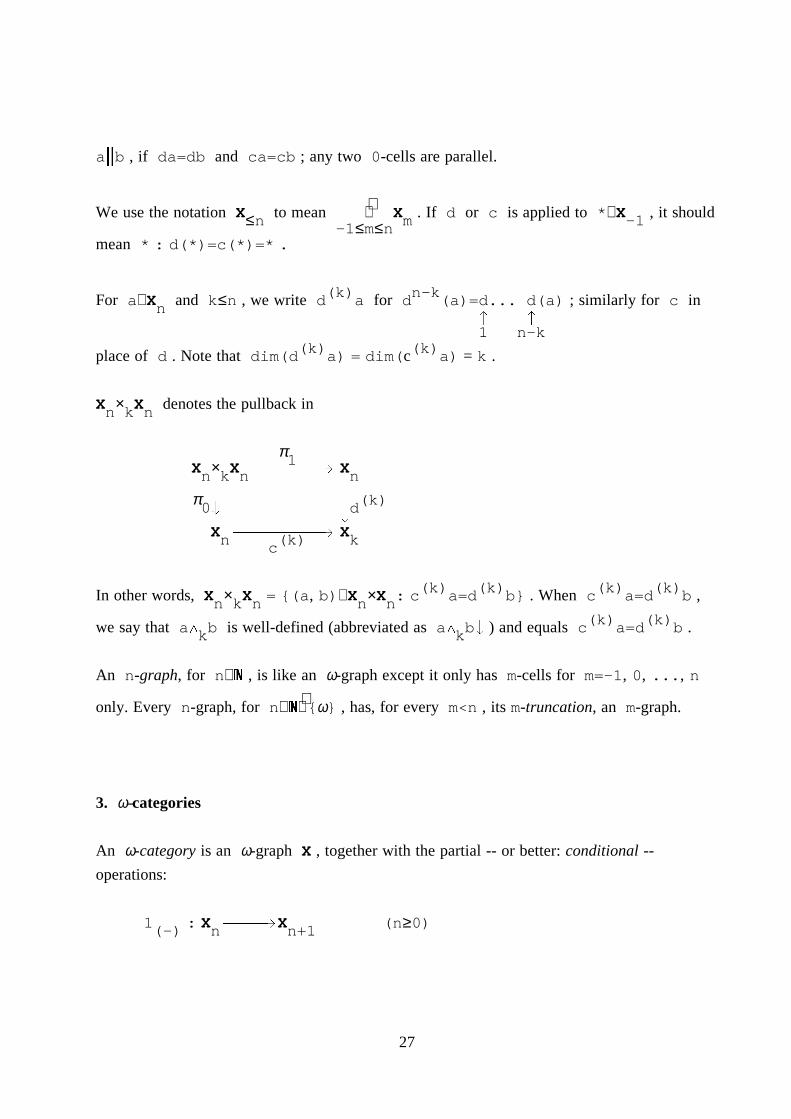
⋅We use the notation X to mean ∪ X . If d or c is applied to *∈ X , it should≤n m -1-1≤m≤nmean * : d(*)=c(*)=* .

(k) n-kFor a∈ X and k≤n , we write d a for d (a)=d... d(a) ; similarly for c inn O O1 n-k

(k) (k)place of d . Note that dim(d a) = dim(c a) = k .

X × X denotes the pullback inn k n

π1X × X A��@ Xn k n n

π � � (k)0P �dPX A��@ Xn (k) kc

(k) (k) (k) (k)In other words, X × X = {(a, b)∈ X ×X : c a=d b} . When c a=d b ,n k n n n(k) (k)we say that aU b is well-defined (abbreviated as aU bP ) and equals c a=d b .k k

An n-graph, for n∈ � , is like an ω-graph except it only has m-cells for m=-1, 0, ..., n

⋅only. Every n-graph, for n∈ �∪ {ω} , has, for every m<n , its m-truncation, an m-graph.

3. ω–categories

An ω-category is an ω-graph X , together with the partial -- or better: conditional --

operations:

1 : X A��@X (n≥0)(-) n n+1

27

# : X × X A��@X (n>k≥0)k n k n n

(a, b) ��@a# bkaU bPk

satisfying the conditions given below.

(n) (k)Let us write, recursively, 1 for 1 for a∈ X and n>k , with 1 = a ;a (n-1) k a def1a(n) (n)we have 1 ∈ X . Any cell of the form 1 with a∈ X is a k-to-n identity cell.a n a k

(Thus, # is composition in the "geometric" order of arguments; we may write bv a fork ka# b . However, the "geometric" # notation is preferred, and when below the juxtapositionk k

(n) (n)ab , or the form a ⋅b occurs, it will stand for 1 # 1 witha k bn=max((dim(a),dim(b)) and k = min(dim(a),dim(b))-1 .)

The axioms on the operations are as follows; throughout, n>k≥0 and a, b, e, f∈ X arenarbitrary.

Domain/codomain laws:

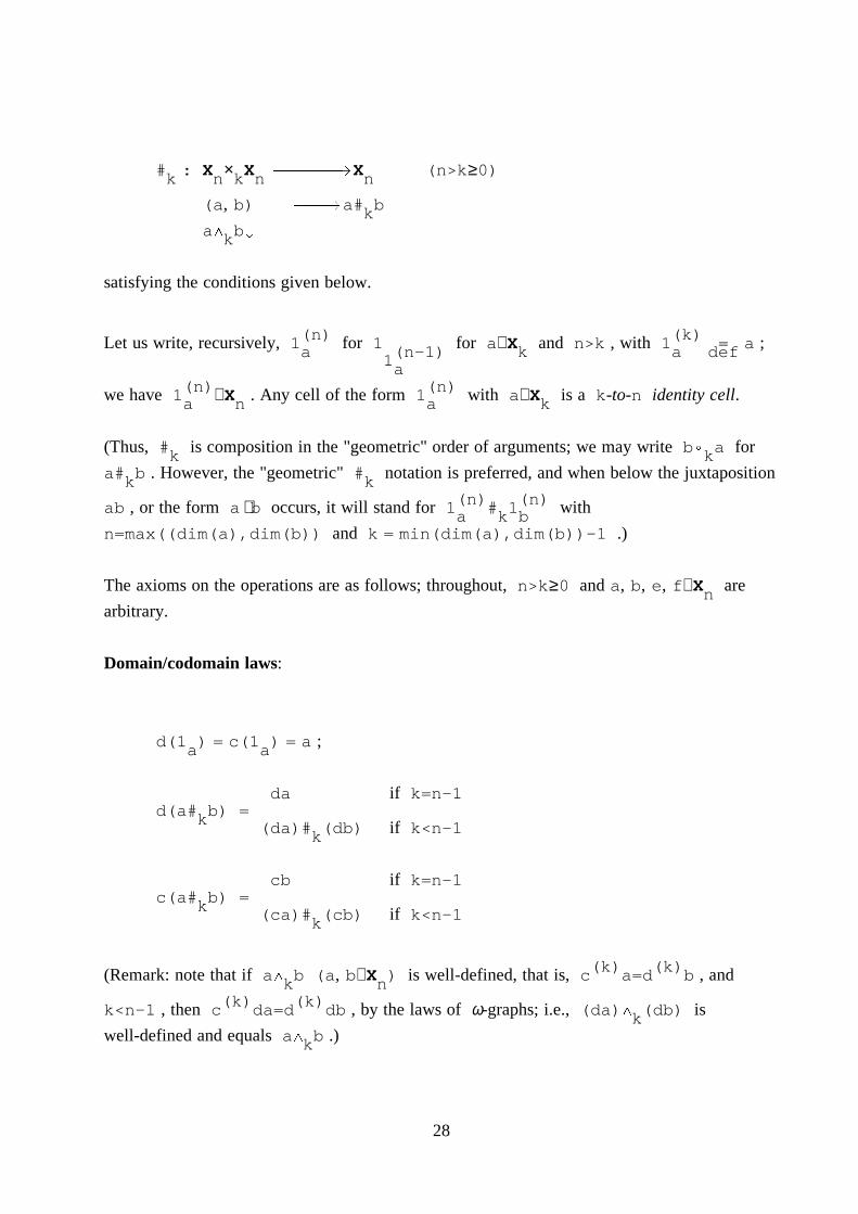
d(1 ) = c(1 ) = a ;a a

da if k=n-1d(a# b) =k (da)# (db) if k<n-1k

cb if k=n-1c(a# b) =k (ca)# (cb) if k<n-1k

(k) (k)(Remark: note that if aU b (a, b∈ X ) is well-defined, that is, c a=d b , andk n(k) (k)k<n-1 , then c da=d db , by the laws of ω-graphs; i.e., (da)U (db) isk

well-defined and equals aU b .)k

28

Left unit law:

(n)1 # b = b(k) kd b

Right unit law:

(n)a # 1 = a .k (k)c a

Two–sided unit law:

1 # 1 = 1a k b a# bk

provided that a# b is well-defined.k

Associative law:

(a# b)# e = a# (b# e)k k k k

provided that a# b and b# e are well-defined.k k

(Remark: note that if a# b and b# e are well-defined, thenk k(k) (k) (k)c (a# b) = c b = d e =k

and

(k) (k) (k)c a = d b = d (b# e) ,k

thus both sides of the associativity identity are well-defined. In other words, under the

conditions for the associative law,

29

(a# b)U e = bU e and aU (b# e) = aU b .k k k k k k

Note, moreover, that, even before we know that they are equal, the two sides are seen to be

parallel.)

(Middle Four) Interchange law:

(a# b)# (e# f) = (a# e)# (b# f)k # k # k #provided that k≠ # , and the four "simple composites" involved are well-defined.

(Remark: we assume that aU b , eU f , aU e , bU f are well-defined; in other words,k k # #(k) (k) (k) (k)c a=d b , c e=d f , (1)

( #) ( #) ( #) ( #)c a=d e , c b=d f . (2)

Because of the obvious symmetry in the interchange identity, we may assume that, e.g., k< # .

It then follows that

(k) (k) ( #) (k) ( #) (k)c a = c c a = c d e = c e ,

(k) (k)and similarly, d (b) = d (f) . Thus

(k) (k) (k) (k)c a = c e = d (b) = d (f) . (3)

Since k< # , we have

( #) ( #) ( #)c (a# b) = c (a)# c (b) ,k k( #) ( #) ( #)d (e# f) = d (e)# d (f)k k

which are equal by (2), hence, the left-hand side of the interchange identity is well-defined.

30

Since

(k) (k) (k) (k)c (a# e) = c (a) = d (b) = d (b# f)# #(by (3)), the right-hand side of the interchange identity is well-defined.

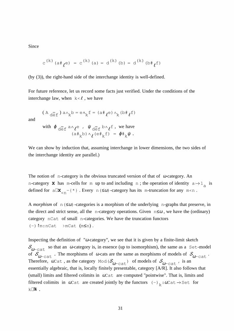
For future reference, let us record some facts just verified. Under the conditions of the

interchange law, when k< # , we have

( A = ) aU b = eU f = (a# e)U (b# f)def k k # k #and

with ϕ = aU e , ψ = bU f , we havedef # def #(a# b)U (e# f) = ϕ# ψ .k # k k

We can show by induction that, assuming interchange in lower dimensions, the two sides of

the interchange identity are parallel.)

The notion of n-category is the obvious truncated version of that of ω-category. An

n-category X has m-cells for m up to and including n ; the operation of identity a�@1 isadefined for a∈ X -{*} . Every n(≤ω)-category has its m-truncation for any m<n .<n

A morphism of n(≤ω)-categories is a morphism of the underlying n-graphs that preserve, in

the direct and strict sense, all the n-category operations. Given n≤ω , we have the (ordinary)

category nCat of small n-categories. We have the truncation functors

(-)�m:nCatA�@mCat (m≤n) .

Inspecting the definition of "ω-category", we see that it is given by a finite-limit sketchS so that an ω-category is, in essence (up to isomorphism), the same as a Set-modelω-catof S . The morphisms of ω-cats are the same as morphisms of models of S .ω-cat ω-catTherefore, ωCat , as the category Mod(S ) of models of S , is anω-cat ω-catessentially algebraic, that is, locally finitely presentable, category [A/R]. It also follows that

(small) limits and filtered colimits in ωCat are computed "pointwise". That is, limits and

filtered colimits in ωCat are created jointly by the functors (-) :ωCatA@Set forkk∈ � .

31

Analogous statements can be made for nCat (n∈ � ).

The functor (-)�n:ωCatA�@nCat has a left adjoint (for the simple reason that it is a

limit-preserving functor between essentially algebraic categories), call it

(ω) (ω)(-) :nCatA�@ωCat , which is easy to describe. For X∈ nCat , X has its

(ω)n-truncation equal to X ; for all k>n , the k-cells of X are all n-to-k identity cells;

their composition law is the only possible one.

(ω)Because of the innocence of the functor (-) :nCatA@ωCat , it is often the case that

(ω)we regard the n-category X as identical to the corresponding ω-category X .

For any m<n∈ � , we have the truncation functor (-)�m:nCatA@mCat , and its left adjoint

(n)(-) , with properties analogous to the the above.

4. Adjoining indeterminates

Let X be an ω-category. Let U be a set, and u�@du, u�@cu two functions UA�@kXksuch that, for each u∈ U , dukcu . The elements of U are regarded as "indeterminate"

elements, each u∈ U of dimension n+1 if dim(du)=dim(cu)=n , waiting to be adjoined

to X as a new element, fitted into the slot given by du and cu as u:duA@cu . The pair

(d,c) of functions is sometimes referred to as the attachment of U to X .

Suppose X and U=(U, d, c) are given as above.

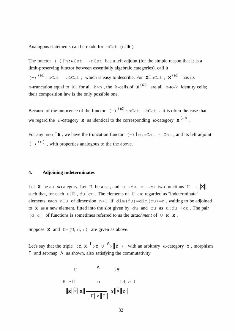
Γ ΛLet's say that the triple (Y, XA�@Y, UA�@kYk) , with an arbitrary ω-category Y , morphism

Γ and set-map Λ as shown, also satisfying the commutativity

ΛUA��@Y� �� ⟨ d, c ⟩ � { � ⟨ d, c ⟩� �P PkXk×kXkA��@kYk×kYkkΓk×kΓk32

is an extension of X by U . In an extension of X by U , we have the elements of U

"realized" as real cells, with domain and codomain that are given by what the (d, c)-data on

U and the "injection" of X into the extension say they should be.

Extensions of X by U form a natural category Ext(X; U) : an arrow Γ Λ Γ Λ (Y, XA�@Y, UA�@kYk)A��@(Y, XA�@Y, UA�@kYk)is a morphism YA�@Y that makes the following two diagrams commute:

Γ Y Λ kYk��B ��BL � L �XG � UG �� P �� Ph h Γ Y Λ kYkA free extension X by U is an initial object of Ext(X; U) . It easy to see that Ext(X; U)

is an essentially algebraic category. Therefore, the free extension of X by U exists and is

determined up to isomorphism. It is denoted

Γ Λ(X[U], XA�@X[U], UA�@kX[U]k) .

Extensions in our present sense may be regarded in a slightly different way. The data (X; U)

-- meaning (X;U,d,c) as above -- form, with all parameters varying, a category F of

"(extension) frames": an arrow

(X; U)A��@(Y; V)

Γ Λis meant to be a pair (XA�@Y , UA�@V) making the diagram

33

ΛUA��@V� �� ⟨ d, c ⟩ � { � ⟨ d, c ⟩� �P PkXk×kXkA��@kYk×kYkkΓk×kΓkcommute; composition in F is the evident one. Note that every Y∈ ωCat gives rise to the

"tautological" frame τ(Y) = (Y;(kYk-{*},d,c)) , with the d and c maps thosedefΓ Λgiven by the ω-category Y . We see that an extension (Y, XA�@Y, UA�@�Y�) of X by U

to Y is the same as a map (X; U)A�@τ(Y) . All this amounts to saying that "free extension

is left adjoint to tautological frame":

τM��NF > ωCat ,A��@E(X;U)��@ X[U]

Γ Λthe pair (XA�@X[U], UA�@kX[U]k) being the component at (X; U) of the unit of the

adjunction E!τ . This is useful: we see that, for any map (Γ, Λ):(X; U)A@(Y; V) of

frames, we have the corresponding "canonical" map E(Γ, Λ):X[U]A@Y[V] . Thus, for

instance, if we have two sets U⊂ V of indeterminates for X , with the d and c functions on

U the restrictions of those for V , we have the canonical map X[U]A�@X[V] , given asE(Id ,incl ) .X U⊂ V

We collect some plausible, and mostly easy, facts about free extensions.

Suppose we have frames (X; U) and (X; V) , with the same underlying ω-category X . We

can do two things. On the one hand, we can consider X[U] , and consider V as

indeterminates in X[U] , by using, for d:VA�@kX[U]k , the composite

d ΓVA��@kXkA��@kX[U]k , and similarly for c . This gives rise to the free extension

⋅X[U][V] . On the other hand, we may look at U∪ V (assuming, of course, that U and V

are disjoint) , with the obvious d and c on this set, as a new set of indeterminates for X ;

⋅this gives rise to X[U∪ V] . The claim is that

34

⋅(1) X[U][V] and X[U∪ V] are canonically isomorphic.

⋅For instance, one way of seeing this is to see that X[U∪ V] has the universal property of

⋅X[U][V] . More precisely, we have the canonical arrow F:X[U]A��@X[U∪ V] as

i Λ ⋅explained above; and we have Λvi:VA�@U∪ VA�@kX[U∪ V]k , with i the inclusion; we

can show that

⋅ F ⋅ Λvi ⋅(X[U∪ V], X[U]A��@X[U∪ V], VA��@kX[U∪ V]k)is initial in Ext(X[U], V) .

(2) The canonical morphism Γ:XA�@X[U] is an injection, and the images of Γ and

Λ:UA�@kX[U]k are disjoint. Moreover, a composite of two elements in X[U] belong to

the image of Γ only if both factors belong to the image of Γ .

(Later we'll see that Λ:UA�@kX[U]k is injective too.)

For the proof, see the appendix.

A subωcategory of an ω-cat Y is an ω-cat S for which kSk⊆ kYk , and the inclusion

mapping i:kSkA@kYk induces a (unique) morphism of ω-cats. The subωcategories of Y

are in a bijective correspondence with subsets S of kYk which are closed, that is closed

under the operations of domain, codomain, identity, and (well-defined) compositions in Y .

For a morphism F:XA@Y of ω-cats which is a monomorphism (equivalently (!), injective on

all cells), the concept of image of F is well-defined: we can take the subset

S={Fa:a∈ �X�} of kYk , and define the ω-cat operations domain, codomain, identity and

compositions on S compatibly with both X and Y , making up S , a subcategory of Y .

We have that, for any monomorphism F:XA@Y of ω-categories, there is a unique

factorization F=jvi such that j is an isomorphism, and i is an inclusion of a

35

subωcategory.

We can combine assertions (1) and (2) into

(3) Given ω-category X , and sets U and V of indeterminates attached to X , the

attachment of U being the restriction of that for V , the canonical map X[U]A��@X[V] is

an injection.

The reason is that X[V]=X[U∪ (V-U)] is, by (1), the same X[U][V-U] , and

X[U]A�@X[U][V-U] is, by (2), an injection.

We also have the following corollary of (1) and (2), which is something one really cannot do

without:

(4) The canonical map Λ:UA@kX[U]k is an injection.

Proof. Let u be any fixed element of U . By (2), we may regard X[U] as

X[U-{u}][{u}] . We have the canonical maps Λ :{u}A�@X[U-{u}][{u}] and1Γ :X[U-{u}]A�@X[U-{u}][{u}] . By (2), the images of Λ and Γ are disjoint. It is1 1 1clear Λ(u)=Λ (u) and Λ�(U-{u}) factors through the map �Γ � . It follows that1 1Λ(u)∉ Λ(U-{u}) (direct image). Since u∈ U was arbitrary, the assertion follows.

It is important that Y=X[U] , initially given by an "externally attached" set U , can in fact be

written as X[V] where V=Λ(U) , the direct image of U under Λ : V is a set of cells in

Y , and its attachment to X -- which is, or rather, may assumed to be, a subωcategory of Y

(see (2)) -- is given by the "internal" domain and codomain functions of Y . This is true

because of (4).

Next, I am going to reformulate (3) as the statement saying that if, in a given ω-cat of the

36

form X[V] , I take a subset U of V , and form the subcategory X ⟨ U ⟩ generated by X∪ U ,

then X ⟨ U ⟩ is in fact X[U] , the extension of X by U . However, I will do it carefully.

Let Y be an ω-category, X a subωcategory of Y , and U a set of cells in Y . Let X ⟨ U ⟩the least subset of kYk that contains kXk∪ U and closed under the operations of taking

identities and well-defined composites. Note that, for any fixed n , X ⟨ U ⟩ is the least setndefZ such that X ⊆ Z , U ⊆ Z (U = U∩Y ) , b∈ X ⟨ U ⟩ �� 1 ∈ Z , and a, b∈ Z,n n n n n-1 b

a# bP �� a# b ∈ Z . If it is the case that for all u∈ U , we have du, cu∈ X , then it isk keasy to see that X ⟨ U ⟩ becomes also closed under "domain" and "codomain", and thus, it is a

subωcategory of Y .

This last situation takes place when Y is the free extension Y=X[V] , with V a set of

indeterminates internally attached to X (in particular, kXk,V⊆ kYk ) and U is a subset of

V . What we just said applies, and X ⟨ U ⟩ is a subωcategory of Y . I claim that, in fact,

X ⟨ U ⟩ =X[U] , meaning that the inclusion XA@X ⟨ U ⟩ has the universal property of the free

extension Γ:XA@X[U] .

Consider an abstract instance of the free extension Γ:XA@X[U] . The universal property of Γ gives us a map Γ:X[U]A@X[V] that is the identity on the set kXk∪ U . By (3), Γ isinjective. Its image is clearly the same as X ⟨ U ⟩ . Therefore, Γ induces an isomorphism ≅Γ:X[U]A��@X ⟨ U ⟩ . We have shown that X[U]≅ X ⟨ U ⟩ as promised.

We have shown:

(5) Given a free extension Y=X[V] , with internal indeterminates V , then for any subset

U of V , X ⟨ U ⟩ is the free extension X[U] of X by U . Moreover,

X[V] = X[U][V-U] .

1 nWe now consider finite iterations X[U ]...[U ] , and infinite iterations� 1 nX[U] = X[U ]...[U ]... of the operation of forming free extensions.

37

Let X be an ω-cat, and assume we have the following (in what follows, superscripts such as

nin X do not mean exponentiation):

n 0the ω-categories X for n∈ � , with X =X ;

n n-1for n∈ �-{0} , the set U of indeterminates attached to X (by "parallel" maps

dnA��@ n-1 n n-1 nU kX k ) such that X = X [U ] .A��@c

n n-1 n n n nWe then have the injective maps (see (2) and (4)) Γ :X A�@X , Λ :U A�@�X � .

We can form the directed colimit� nX[U] = colim X .def n∈ �Filtered colimits in ωCat are created by the forgetful functor to Set . It follows that the�colimit coprojections ϕ :X A@X[U] are injective.n n

n ⋅ nFor convenience, we assume that the sets U are pairwise disjoint. We let U = abc U .n∈ �-{0}�By iterating (4), we get that the induced map ψ:UA@kX[U]k is injective. Let V=ψ(U) , the� � �direct image of ψ . Thus, we have that Y=X[U] can also be written as Y=X[U]=X[V] ,� n �with the obvious meaning for V= ⟨ V ⟩ ; the attachment of V is internal to Y (thatn∈ �-{0}

is, the attachment values dv and cv are the same as dv and cv in the sense of Y ).

nLet Y be an ω-cat, X a subωcat. Consider a subset U of kYk , for each n≥1 , such

n ≤n-1 ≤n-1 mthat u∈ U implies that du,cu∈ X ⟨ U ⟩ (where U =abc U ); in this case wem≤n-1� n nsay that the system U= ⟨ U ⟩ is self-contained. If so, then we have that, with U=abcU ,n nO ≤nX ⟨ U ⟩ is a subωcat of Y ; also, X ⟨ U ⟩ = abcX ⟨ U ⟩ (directed union).

n� �Note that if Y=X[V] , an internal iterated free extension, then we have that V is� m nself-contained and Y=X ⟨ V ⟩ ; moreover the system V is disjoint: V ∩V =∅ for m≠n (see

38

(2)). � n �(6) Let Y=X[V] be an internal iterated free extension, V=abcV , U a disjointnnself-contained system of elements in Y with total set U=abcU =V . Then Y is the iterated

n�free extension X[U] of X .

≤n 1 nProof. Using (5), by induction on n , we prove that X ⟨ U ⟩ =X[U ]...[U ] , with the

obvious canonical inclusions. Passing to the colimit makes the assertion clear.� � �Note that (6) allows us to write X[V] as X[V] , with V the total set of V , since X[V]

depends really only on V and X .

We have the following generalization of (5):�(7) Let Y=X[V]=X[V] , an internal iterated free extension as explained above,

n n � nV=abcV , and let, for each n≥1 , U ⊆ V , and assume that U = ⟨ U ⟩ is disjoint andnn � �self-contained. For the total set U of U , X ⟨ U ⟩ is the iterated free extension X[U]=X[U]

of X by U . Moreover, X[V]=X[U][V-U] .

n n nNote that we did not assume U ⊆ V , only U ⊆ V .

n nProof. First, we show the assertion under the stronger assumption U ⊆ V for all n .

Secondly, we reduce the general case to said special case as follows. Given the data as in (6),�we construct a disjoint self-contained system W ( W ∩W =∅ for n≠m ) with total set W=Vn mn n �such that, for each n , U ⊆ W . This construction is left as an exercise. By (6), Y=X[W] ,

39

and we have made the promised reduction.

We will need the operation of freely adjoining n-dimensional indeterminates in a set U to

an (n-1)-category X , to obtain the n-category X[U] . This is essentially a special case of

(ω)our construction above, since X may be regarded to be an ω-category, namely X . In

(ω)fact, it is not necessary to bring in the object X , since everything we want has an

obvious, direct expression in terms of (n-1)-categories and n-categories.

We want to state a result to the effect that, from X[U] as a mere ω-category, under certain

conditions we can recover X and U .

Let Y be any ≤ω-category.

(n) (n)Recall the notation 1 . For a k-cell a , k<n , we say that 1 is a k-to-n identitya acell.

Let n∈ � . We consider the following condition (C ) on Y :n

(C ) Whenever #<n , k<n , x, y∈ Y , and x# y is well-defined, if x# y is an n # #k-to-n identity, then both x and y are k-to-n identities.

Condition (C ) says that Y is the "opposite" to being an n-groupoid.n

Let n∈ � and x∈ Y . Let us say that x is indecomposable if the following hold:n

(i) x ≠ 1 for all y∈ Y ; andy n-1

(ii) whenever y, z∈ Y , k<n and x=y# z , we have that either y or z is an kk-to-n identity (and x=z , respectively, x=y ).

(8) Proposition For any (n-1)-category X satisfying (C ) , and any setn-1U of n-indeterminates attached to X , we have the following:

40

(8.1) X[U] satisfies (C ) .n

(8.2) The canonical map Λ:UA�@(X[U]) is one-to-one.n

(8.3) The image of Λ consists exactly of the indecomposable n-cells of

X[U] .

41

(8.4) The canonical inclusion Γ:XA@X[U] is an isomorphism onto the

(n-1)-truncation of X[U] .

(The conclusions (8.2) and (8.4) are already known, under more general conditions.)

For the proof, which is similar to that of (2) but more complicated, see the appendix.

Let us note that without assuming (C ) for X , even when we drop (8.1) from then-1assertion, (8) becomes false: take the example when n=2 , and X is a groupoid.

42

5. Computads �A computad is an ω-category of the form ∅ [U] , that is, an iterated free extension of the

empty (initial) ω-category ∅ (which still has *∈ ∅ ).-1

An alternative definition, equivalent to the first one, is as follows.

n-computads, for n∈ � , are defined recursively; each n-computad is, in particular, an

n-category.

A 0-computad is a 0-category: a set.

An n-computad is any n-category isomorphic to one of the form X[U] , where X is an

(n-1)-computad, and U is a set of n-indeterminates attached to X .

A computad is an ω-category whose n-truncation is an n-computad, for each n∈ � .

It is important to realize that the indeterminates are not "lost" in the wording of the definition.

Indeed, as a consequence of 4.(8), the indeterminates of a computad are exactly the

indecomposable cells.

To emphasize what we just said, we rephrase the definition as follows.

Let X be an ω-category. Let X�n the n-truncation of X , and let U denote the set of allnn-indecomposables in X , attached to X internally. Then X is a computad iff, for allnn≥1 , (X , Γ:X A@X , Λ:U A@�X �) , with Γ , Λ denoting inclusions, is a freen n-1 n n nextension of X by U .n

A corollary is

(1) If X is a computad, and X’ is an ω-category isomorphic to X , then X’ is a

≅computad as well. Moreover, any isomorphism f:XA�@X’ of ω-categories between

computads X , X’ takes any indeterminate in X to an indeterminate in X’ .

42

A morphism F:XA�@Y of computads X , Y is a morphism of ω-categories that maps

indeterminates to indeterminates. We obtain the category Comp of small computads, with a

non-full inclusion Φ:CompA@ωCat . By (2), Φ is full with respect to isomorphisms: the

* * * *restriction Φ :Comp A@ωCat is a full inclusion (for a category C , C is its underlying

groupoid).

For a computad X , QXR denotes the set of its indeterminates: QXR= $ QXR =abcQXR ,n nn∈ � n∈ �where QXR is the set of n-indeterminates (indecomposables of dimension n ). We have thenforgetful functor Q-R:CompA@Set .

A special case of 4.(8) is

(2) Let X be a computad, U⊆ QXR ; write U =U∩QXR . Assume that u∈ U impliesn n nthat du,cu∈ ∅ ⟨ U ⟩ (for this, we say that U is a down-closed set of indeterminates).n-1Then ∅ ⟨ U ⟩ , the subωcat of X generated by U , is a computad, and Q∅ ⟨ U ⟩ R=U .

(2) tells us how to generate some of the subobjects of an object of the category Comp . To

show that we obtain all subobjects in this way requires more work. To anticipate that result,

for any computad X , we call an subωcat of X of the form ∅ ⟨ U ⟩ with U a down-closed

subset of QXR a subcomputad of X . By (2), any subcomputad is a computad on its own

right.

(3) The category is small-cocomplete, and the functors Φ:CompA@ωCat ,Q-R:CompA@Set preserve all small colimits.

This is essentially clear from the definitions; for details see the appendix.

(4) The functor Q-R:CompA@Set is faithful and reflects isomorphisms.

43

Proof: see appendix.

In what follows, we let X be a computad; a, b, ... are arbitrary elements of X ,

u, ..., x, ... are indeterminates of X .

The following is an important tool.

(5) Lemma There is a unique function

supp = supp :�X�A��@P(QXR)X

satisfying the equations

supp(*) = ∅supp(x) = {x} ∪ supp(dx) ∪ supp(cx) (x∈ QXR)supp(1 ) = supp(a) (a∈ X)asupp(a# b) = supp(a) ∪ supp(b) (a,b∈ X)k

Moreover, for all a∈ X ,

supp(da) , supp(ca) are subsets of supp(a) ;

supp(a) ⊆ Q XR ;≤dim(a)supp(a) ⊆ Q XR �� a=1 for some b .≤dim(a)-1 bsupp(a) is a finite set.

Proof: see the appendix.

We think of supp(a) , the support of a , as the set of indeterminates "occurring" in a .

Before we proceed, let us make a general remark. The fact that X=∅ ⟨ QXR ⟩ translates into

the following "computad induction" principle. Assume P is a property of elements of X ,

44

P⊆ �X� . Suppose we have the following four conditions satisfied:

(i) *∈ P ;

(ii) for all x∈ QXR : X ⊆ P �� x∈ P ;<dim(x)(iii) for all b∈ X : b∈ P �� 1 ∈ P ;≥0 b(iv) for all b, e and k : (b# eP & b∈ P & e∈ P) �� b# e ∈ P .k k

Then P=�X� .

Skeptics may see the appendix.

(6) (i) supp(a) is a down-closed subset of QXR and a∈ ∅ ⟨ supp(a) ⟩ .

(ii) Given F:XA�@Y in Comp , let a∈ X . Then the direct image of supp (a)Xunder F is supp (Fa) . In other words, F induces a surjective mapYsupp (a)A�@supp (Fa) .X X

Proof: straight-forward computad induction; see the appendix.

(7) Suppose X is a subcomputad of Y .

(i) For a∈ X , supp (a)=supp (a) .X Y(ii) If a∈ X , then supp (a) ⊆ QXR . Hence, supp (a) is the leastY Y

down-closed subset U of QYR for which a∈ ∅ ⟨ U ⟩ .

(iii) A subset U of QYR is down-closed iff for all u∈ U , we have

supp (u)⊆ U .Y(iv)(!) Whenever a, b∈ Y , a# b is well-defined and a# b ∈ X , then ak k

and b both belong to X .

Proof. (i) is a special case of 6.(ii). (ii) and (iii) follow from (i) . To prove (iv), assume the

assumptions. supp (a# b) = supp (a# b) = supp (a) ∪ supp (b) , hence,X k Y k Y Ysupp (a) ⊆ supp (a# b) ⊆ QXR . Since a∈ ∅ ⟨ supp (a) ⟩ , we have a∈ ∅ ⟨ QXR ⟩ =Y X k YX . Similarly, b∈ X .

45

(8) Let F:XA��@Y be a map of computads.

(i) F(QXR) , the direct image of QXR under F , is a down-closed set of

indeterminates of Y .

(ii) For any down-closed subset V of QYR , the inverse image of V ,

-1QfR (V)={x∈ QXR:f(x)∈ V} is down-closed in X . (In (10)(ii) below, we'll see that, in

-1 -1fact, QfR (V)=f (V) .)

(iii) Pullbacks of diagrams in Comp in which one of the arrows is a monomorphism

are preserved by the forgetful functor Q-R:CompA@Set .

(iv) Small colimits in Comp are stable under pullbacks along monomorphisms.

Proof. (i) and (ii) follow from (6) and (7); (iii) follows from (ii). (iv) follows from (iii) and (3)

and (4).

(9) Let F:XA��@Y be a map of computads.

(i) F is factored in the category Comp uniquely as F=ivP where i is

the inclusion map of a subcomputad of Y , and QPR is surjective.

(ii) F is a monomorphism in Comp iff it (that is, Φ(F) for the inclusion

Φ:CompA@ωCat ) is a mono in ωCat iff QFR is injective.

(iii) F is an epimorphism in Comp iff QFR is surjective.

(iv) The subobjects of a computad X , in the sense of the category Comp ,

are the same as (are in a bijective correspondence with) the subcomputads of X .


(10) Let F:XA@Y be a morphism of computads, n∈ � , a∈ X . Thenn

(i) a = 1 �� Fa = 1da Fda(ii) a is an indeterminate �� Fa is an indeterminate.

46

Proof. The left-to-right implications are clear.

For �� in (i): If Fa=1 , then supp(Fa)⊆ QYR ; by (7), it follows thatFda n-1supp(a)⊆ QXR , hence, by (5), the third "moreover" statement, a=1 .n-1 da

(n)For (ii), first of all note that by (i), if b=Fa , and b=1 , a k-to-n identity, thenf(n)a=1 , for a suitable e , and Fe=f . Assume a is not an indeterminate. We use 4.(8):e

we have that a is not indecomposable, i.e., a=a # a where neither a nor a is a1 k 2 1 2k-to-n identity. Then, by what we just said, neither Fa nor Fa is a k-to-n identity,1 2and Fa=Fa # Fa is not indecomposable, i.e., not an indeterminate.1 k 2

Let us call a computad X finite if QXR is a finite set.

Let a∈ X . Since supp(a) is down-closed, Supp(a) = ∅ ⟨ supp(a) ⟩ is adefsubcomputad of X . Since QSupp(a)R=supp(a) , Supp(a) is a finite computad.

Given two finite subcomputads ∅ ⟨ U ⟩ , ∅ ⟨ V ⟩ , defined by the finite down-closed sets

U, V⊆ QXR , U∪ V is finite and down-closed (obviously, any union of down-closed sets of

indets is down-closed). We can form the finite subcomputad ∅ ⟨ U∪ V ⟩ . This shows that the

set S (X) of finite subcomputads of X ordered by inclusion is directed.fin

The union of all the elements of S (X) is X , and this union is a colimit (see (3)). Wefinhave shown that every computad is a filtered colimit of finite computads.

It is easy to see that a finite computad is finitely presentable (fp) object of Comp . In fact,

since a retract, in fact, any subcomputad, of a finite computad is finite, the finite computads

are exactly the fp ones.

Since, by (3), Comp has all small filtered colimits, we have shown that Comp is an

ℵ -accessible category. Since it is small-cocomplete ((3)), it is a locally finite presentable (lfp)0category. In particular, Comp is small-complete.

47

Unlike in most of the lfp categories appearing in practice, in Comp , it is not the limit

structure, but the colimit structure, that is familiar. The limit structure is complicated, and, to a

large extent, "unknown". The terminal computad is "large"; its set of indeterminates is

countably infinite. Although, as we later show, it is a structure with a recursively solvable

word problem, it is "very complicated".

(11) Arbitrary intersections and unions of down-closed sets of indets are again down-closed.

The down-closed sets of the form supp(x) , x an indet are join irreducible:

supp(x)=abcU , each U down-closed, imply that there is i such that supp(x)=U .i i iiAll down-closed sets are unions of ones of the form supp(x) , x an indet. The subobject

lattice of X is a completely distributive lattice.

We like to call arbitrary elements (cells) of a computad pasting diagrams (pd's).

Next, we introduce a concept of "multiplicity" of an indet in a pd a . Let X be a computad.QXRThe elements of � are the multisets of indeterminates. The elements of the subsetQXR � �QXR ⋅� of � are the vectors (functions) m= ⟨ m ⟩ ( m =m(x) ) for whichx x∈ QXR xonly finitely many m is non-zero; these are the finite multisets of indets. Multisets form anxAbelian group under componentwise addition + ; finite multisets form a subgroup.

Obviously, the Abelian group QXR ⋅� is the free Abelian group generated by the elements ofQXR ; accordingly, we may write ⟨ m ⟩ as � m ⋅x . Still, we prefer thex x∈ QXR xx∈ QXRxfunctional notation ( ) to m ⋅x .m�The multiset m is non-negative if m ≥0 for all x . We also use the partial orderx� � � �m≤n �� n-m is non-negative.

In the next proposition, we define the content [a] of a pd a in a computad X . [a] is

intended to be the multiset of all the indeterminates in a , with each indet counted with the

proper multiplicity. The definition given here does not have a certain expected property:

48

(*?) When X is a computope, [m ] (u) = 1 for all u∈ QXRX X

(computopes will be explained in the next section). I do not know if there is a content function

with (*) and all the properties (v) to (x) in the next proposition.

(12) Proposition There is a unique function

[-]=[-] : X A��@QXR ⋅�X ≥-1

satisfying the following equalities:

(i) [*] = 0

x(ii) [x] = ( ) + [dx] + [cx] ( x∈ QXR )1(iii) [1 ] = [a] ( a∈ X )a ≥0(iv) [a# b] = [a] + [b] - [aU b] ( a, b∈ X , a# b P )k k ≥1 k

Moreover, we have

(v) [a] ≥ 0

(vi) [da],[ca] ≤ [a]

(vii) [a], [b] ≤ [a# b]k(viii) [a](x) > 0 �� x∈ supp(a)(ix) For any F:XA�@Y in Comp and any a∈ X , y∈ QYR ,≥-1

[Fa] (y) = � [a] (x) .Y Xx∈ QXRFx=y

(x) x∈ supp(a) �� [x]≤[a] .


49

6. Multitopes and computopes

As an application of 1.(4), we discuss multitopes and multitopic sets.

Let X be a computad. An indeterminate x∈ QXR is many-to-one if cx is an indeterminate.

X itself is many-to-one if all indeterminates in X are so.

The full subcategory of Comp on the many-to-one computads is denoted Comp . Asm/1usual with subcategories of Comp , we regard Comp as a concrete category, with QXRm/1the set of all indets of X ( X∈ Comp ).m/1

Our starting point is a result that is a consequence of theorems proved in the papers [H/M/P]

and [H/M/Z].

(1) Theorem Comp is a concrete presheaf category.m/1

The shape category of Comp is called the category of multitopes; it is denoted by Mlt .m/1

In some detail, the reasons for the truth of the last theorem are as follows.

In [H/M/P], the concept of multitopic set is introduced. The category MltSet of multitopic

sets is defined, the category Mlt of multitopes is defined, and it is proved that MltSet is

op Mltequivalent to Mlt = Set . Although it is not stated explicitly, it is implicit in[H/M/P] that, in fact, MltSet is equivalent as a concrete category to Mlt , where the

forgetful functor Q-R:MltSetA�@Set is defined as explained in the Introduction, part (C).

On the other hand, in [H/M/Z] it is shown, among others, that MltSet is equivalent to

Comp . Again, it is not explicitly stated, but it is implicit that MltSet and Compm/1 m/1are equivalent as concrete categories, with the same forgetful functors as before.

50

Combining the two facts, we get that Comp and Mlt are equivalent as concretem/1categories.

In section 1, we gave a characterization of concrete categories equivalent to a concrete

presheaf category (see 1.(4)); this will give a characterization of the multitopes mentioned

above. Keeping that characterization in mind, let us call a (not necessarily many-to-one)

computad X a computope if there is x∈ QXR such that (X, x) is a primitive element (see

section 1) of Comp .

Note that the element (X, x) of Comp is principal (see section 1) iff X=Supp (x) .X

Such an x in QXR as in the last sentence, if it exists, is unique, since, for any computad X

and x∈ QXR , Supp (x) has a single indeterminate of the dimension equal to that ofXSupp (x) , namely x itself; hence, Supp (x)=Supp (y) for x, y∈ QXR impliesX X Xx=y . The indet x such that (X, x) is principal is called the main indet of X , and denoted

m . We are justified in using the adjective "principal" in referring to a computad, rather than aXpointed computad (an element of Comp ). Every computope is principal.

For X a computope, any self-map XA@X (in Comp ) is necessarily an isomorphism: we

know that any map (X, m )A@(X, m ) in El(Comp) is an iso, and we just saw that forX Xany f:XA@X , we must have QfR(m )=m .X X

Obviously, a principal computad is finite as a computad. For any finite computad X ,

dim(X) is defined as max{dim(x):x∈ QXR} . For a principal computad X ,

dim(X)=dim(m ) .X

It is clear that if XA@Y is any map of finite computads, then dim(X)≤dim(Y) .

Note the obvious facts that a computad map f:AA@B of principal computads A , B is an

epi iff f is surjective (on indets) iff f(m )=m iff dim(A)=dim(B) .A B

Computopes can be equivalently described as those computads X which are principal, and

for which any epimorphism YA@X from a principal Y to X is necessarily an isomorphism.

51

We let Comtope be the full subcategory of Comp whose objects are the computopes.

*Comtope is defined to be the skeleton of Comtope : any skeletal full subcategory of

*Comtope for which the inclusion Comtope A@Comtope is an equivalence.

We isolate four properties of a variable full subcategory C of Comp ; we will point out that

each property is shared by C = Comp .m/1

(a) C is a sieve in Comp ; if XA@Y is a map of computads, and Y is in C , then

so is X .

(b) C is closed under small colimits in Comp .

(c) If f:AA@B in Comp is surjective, and A∈ C , then B∈ C .

(d) C is a concrete presheaf category.

Note that (d) implies (b), by the (obvious) necessity condition (i) in 1.(4), and the same

condition holding for Comp .

5.(10) immediately implies that (a) is satisfied by Comp .m/1

If F:XA@Y is a map of computads, and x∈ QXR is many-to-one, then F(x)∈ QYR is also

many-to-one. Therefore, if {F :X A@Y} is a jointly surjective (on indets) family ofi i i∈ Imorphisms of computads, and each X is many-to-one, then Y is many-to-one. It followsithat Comp satisfies (b) and (c).m/1

Let C be an, otherwise arbitrary, full subcategory of Comp satisfying (a) above. We observe

that

(1.1) for X in C , and x∈ QXR , to say that (X, x) is a principal, resp. primitive,

element of C is equivalent to saying that (X, x) is a principal, resp. primitive, element of

Comp , i.e., that X is a principal computad and x=m , respectively that X is a computopeXand x=m .X

52

We have noted that, for principal computads, in particular computopes, X and Y , X≅ Y in

*Comp iff (X, m ) ≅ (Y, m ) in El(Comp) . This means that the category C [Comp] ,X Y*constructed in section 1, is isomorphic to Comtope .

* *For any sieve C in Comp , we let Comtope be the intersection Comtope ∩C , a sieveC*(in particular, a full subcategory) in Comtope .

A one-way category L is a category in which there are no "descending" infinite chains

f f f0 1 nK M��NK M��K ... M��NK ...0 1 2 n+1

consisting entirely of non-identity arrows. It follows that L is skeletal, and we can define a

dimension-function dim on objects, taking values that are natural numbers, such that the

presence of a non-identity arrow f:AA@B implies that dim(A)<dim(B) .

A category L is said (here) to be finitary if, for each object B , the sieve

{f∈ Arr(L):cod(f)=B} is a finite set. In section 11, we will prove

*(2) The skeletal category Comtope of computopes is finitary.

opThe quality of being both one-way and finitary is that makes Mlt a FOLDS-signature, in

the sense of [M1]. [M2]. This property of Mlt was evident on its definition already, but here

we see that this is a "necessary quality" of Mlt .

One of the main results of this paper is that the condition 1.(4)(ii)(b) holds in the category

A=Comp .

(3) Theorem If X is any computad, x∈ QXR , then there exist a computope X and a

morphism f:XA@A in Comp such that QfR(m )=x .X

53

The proof will be given in section 11.

The following theorem is a summary, obtained from 1.(4) when we take into account what we

have said in this section so far.

(4) Theorem Suppose that the full subcategory C of Comp is a sieve in Comp

(satisfies (a)). Then C is a concrete presheaf category if and only if C satisfies conditions

(o), (i) and (ii) below.

(o) C is closed under small colimits in Comp (satisfies (b)).

(i) For any computad Z in C :

fA�@(i) if X is a computope, and X Z are maps in Comp such thatZ A�@gQfR(m )=QgR(m ) , then f=g . In particular, every self-map of a computope in C is theX Xidentity.

(ii) For any computad Z in C :

f g(ii) whenever X and Y are computopes, and XA�@ZM�NY areZmaps in Comp such that QfR(m )=QgR(m ) , then X ≅ Y .X Y

* *If so, the shape category of C is isomorphic to Comtope , and Comtope is aC Cfinitary, one-way category.

When C is Comp , we have all of (a), (b), (c) and (d) satisfied. We conclude thatm/1

the category Mlt of multitopes, the shape category of Comp , is isomorphic tom/1the skeletal category of all many-to-one computopes.

The theorem offers some hope for a new and softer proof of the fact that Comp is am/1concrete presheaf category.

Inspired by the example of Comp , we use the following terminology. Let Z be am/1

54

computad, z an indeterminate in Z . If X is a computope, and f:(X, m )A@(Z, z) (inXEl(Comp) ), we say that X is a type for z , z is a specialization of m , and f is aXspecializing map for z (or, for Z if Z is principal). The condition (4)(i) says that, once theZtype is fixed, the specializing map of any z∈ QZR is unique. (4)(ii) says that the type of anyZz∈ QZR is unique up to isomorphism (which, of course, is the most we can expect). We know

(see (3)) that every indet in every computad has at least one type.

One might wish to talk about a type of an arbitrary pd in a computad, not just that of an indet.

However, this is not really more general. Let Z , X be computads, a a pd in Z , α a pd in

X , both of dimension n ; assume Z=Supp (a) , X=Supp (α) . Let x , ξ be "new"Z Xindeterminates, both of dimension n+1 , x attached to Z by dx=cx=a , ξ to X by

dξ=cξ=α . Then we have a bijection of maps, depicted as

X[ξ]A��@Z[x]�� .

XA��@Z :: α�@aThis says that talking about a type for a is the same as talking about a type for the "new"

indeterminate x:aA@a .

In particular,

every hereditarily many-to-one indeterminate (an indet in a many-to-one computad) has

a unique type, and a unique specializing map.

In the logical language of FOLDS (see [M1], [M2]), corresponding to many-to-one computads,

opwe have structures of a fixed FOLDS signature, namely Mlt ; corresponding to the

indeterminates in a computad, we have the elements of the structure; corresponding to the type

of an indeterminate, we have the kind of the element; corresponding to the type together with

the specializing map, we have the dependent sort of the element.

Coming to the example when C is chosen to be Comp itself, (4)(i) fails; in particular,

Comp is not a concrete presheaf category. To show this, first we make some remarks of an

elementary nature.

55

We remind the reader of the Eckmann-Hilton identity. Suppose that, in an ω-category, X is a

0-cell, and u and v are 2-cells, both of the form 1 A@1 . Then all of u# v , v# u ,X X 0 0u# v , v# u are well-defined, and they are all equal. Thus, hom(1 , 1 ) , the set of all1 1 X X2-cells of the form 1 A@1 , is a commutative monoid, and both compositions, # andX X 0# , for 2-cells in hom(1 , 1 ) coincide with the monoid operation.1 X X

Conversely, any commutative monoid M can be turned into a 2-category Z with a single

0-cell, a single 1-cell (the identity), and 2-cells the elements of M , with both compositions

of 2-cells given by the monoid operation.

Let now Y be a computad such that Y has no 1-indet: QYR =∅ . It follows that all 1-pd's1(= 1-cells) in Y are identities, every 2-pd (= 2-cell) in Y is of the form 1 A@1 , andX Xhom(1 ,1 ) is the free commutative monoid on the set of indets in hom(1 ,1 ) as freeX X X Xgenerators. (The universal property of the computad Y played against the 2-category derived

from the appropriate free commutative monoid will give that hom(1 ,1 ) is free as aX Xcommutative monoid).

Let X be the computad generated by the 0-indet X , the distinct 2-indets u, v and w , all

ϕof the form 1 A@1 , and the 3-indet u ⋅vA�@w . I claim X is a computope. First, it isX Xclearly principal, X=Supp(ϕ) . To show that (X,ϕ) is primitive, let Y be a principal computad, Y=Supp(ϕ) with a 2-cell ϕ , and let F:YA@X be a morphism; F(ϕ)=ϕ . There is no 1-indet in Y , since

there is none in X ; what we said above about such computads Y applies. In particular, for some 0-cell X , cϕ and dϕ are elements of the free commutative monoid M=hom(1 , 1 ) . F induces a monoid map F:MA@M for M=hom(1 , 1 ) in X , which, X XX X in addition, maps free generators to free generators. Therefore, since F(cϕ)=cϕ=w and F(dϕ)=dϕ=u ⋅v , we must have that cϕ=w , dϕ=u ⋅v for indets w, u, v∈ M . We see that supp (ϕ)={X, u, v, w, ϕ) and that F induces an isomorphismY ≅ Supp (ϕ)A��@X . Since Y is principal, Y=Supp (ϕ) , and F:YA@X is anY Yisomorphism as needed for the claim. We've proved that (X,ϕ) is primitive.

56

There is the non-trivial automorphism α:XA@X that switches u and v , and leaves all other

indets the same: this works precisely because of the Eckmann-Hilton identity. We have found

a computope with a non-trivial automorphism, as promised.

In fact, the same computope X can be used to show that Comp is not equivalent, even in the

"abstract", non-concrete sense, to any presheaf category. To make the argument below more

interesting, we again make some general observations concerning when a full subcategory of

Comp is, abstractly, a presheaf category.

In any category C , we call small the objects A of C for which C(A, -):CA@C commuteswith colimits. The small objects of C , under the assumption C J C , are the ones that correspond under the equivalence to retracts of the representable functors C(-, X) in C .

We also have that every object in C is a colimit of small objects; this is inherited from thepresheaf category C .

Recall (1.1) above, about the use of the words "principal" and "primitive".

(5) Let C be a full subcategory of Comp . Assume that C is a sieve in Comp (satisfies

(a)), C is closed under colimits in Comp ((b)), and, on its own right, C is a presheaf

category. Then

(i) Every C-small object of C is principal, in particular, small in the sense of

Comp ;

(ii) Every primitive object of C is C-small.

If, in addition, C satisfies (c) above, then

(iii) An object in C is C-small if and only if it is Comp-small.

For the proof, see the appendix.

57

Let us return to our particular computad X introduced above. X is not small in Comp , as it

is shown now.

Let Y be the computad, a variant of X , which is generated by the 0-indet X , the distinct

ϕ2-indets u and w , both of the form 1 A@1 , and the 3-indet u ⋅uA�@w . Let Z beX XSupp (u) . We have the diagram of Comp-morphismsX

FA��@ HZ XA��@Y (6)A��@G

where F, G, H are determined by F(u)=u , G(u)=v , H(u)=H(v)=u . (6) is a colimit

diagram in Comp , since upon applying Q-R to it results in the diagram

u�@uA��@ u�@u, v�@u{X, u} {X, u, v, w}A��@{X, u, w}A��@ w�@wu�@vwhich is a coequalizer diagram in Set . When we "hom" into (6) from X , that is, consider

the diagram

hom(X,F)A��@ hom(X,H)hom(X,Z) hom(X,X)A��@hom(X,Y) ,A��@hom(X,G)

we get A��@∅ {1 , α}A��@{H}A��@ X

(here, α is the non-trivial automorphism of X found above), which, of course, is not a

colimit diagram.

X is not small, but it is primitive in Comp as we saw before. Therefore, by (5)(ii) applied toC=Comp , Comp cannot be a presheaf category. More generally, no C satisfying the

hypotheses of (5) can contain X as an object.

58

7. Words for computads

This section is devoted to a precise formulation of the word problem for computads. It is the

natural formulation, following directly the definition of ω-category given in section 2.

The definition here is but an inessential variant of Jacques Penon's word-oriented, syntactical,

definition of computads (polygraphs) in [Pe].

At the end of the section we give the precise statement of the theorem saying that the word

problem for computads is solvable. The definition of the word-problem for computads is given

here in its most direct manner in order to make the statement of that theorem as natural as

possible. As a matter of fact, in the course of the proof of the theorem later in the paper, we

will have to reformulate the word problem itself into a different, albeit equivalent, form.

The syntax for the word problem for computads is more complicated than the analogous

syntax for free groups, and free constructions in general for algebraic structures of the usual

kind, since the condition of being well-defined for a formal expression denoting a cell of a

higher-dimensional category is non-trivial: it is defined in parallel with the essential

equivalence of expressions.

First, we give "global" definitions for words, their well-definedness and essential equivalence.

The relevant concepts for particular computads will be obtained by taking appropriate

restrictions of the global ones.

Let us mention one important choice made in the definition that may not be a priori the

obvious one. This is that the operations of domain and codomain do not have direct symbolic

representations; rather, "domain" and "codomain" become operations on words (this feature is

also present in Penon's approach).

In this section, no proofs of assertions are given. With the exception of the proof of the

theorem at the end of the section, to be given later, they are all routine.

Words with prescribed dimensions are defined "absolutely freely" in the following inductive

definition. We write W for the set of words of dimension m ; here, m∈ �∪ {-1} .m

W = {*} .-1

59

For n∈ � :

0 ⋅ 1 ⋅ 2W = W ∪ W ∪ W ,n n n nwith

0W = {(0, n, ξ , a, b): ξ ∈ V , a, b∈ W } ,n n-11 ∅ if n=0W =n

{(1, n, a): a∈ W } if n≥1n-12W = {(2, n, k, a, b): 0≤k<n, a, b∈ W }n n

⋅(In other words, W= abcW is the least class for which the above equalities hold. Themm≥-1

parentheses indicate ordered tuples (quintuples, triples, quintuples, respectively) in the

set-theoretic sense. V is the universe of all sets. )

0The elements of W are the pre-indeterminates, or pre-indets, of dimension n . The "pre-" isnthere because in order for a pre-indet to be a real indet it will have to be well-defined,

according to the definition given below. The tuple x=(0, n, ξ , a, b) contains the reference

to the fact that we now are talking about an indeterminate (the zero up front); n gives the

dimension; next it has an arbitrary name ξ , to ensure that we have an unlimited supply of

indets; a is to be the domain of x , b the codomain. Of course, the "problem" is that,

eventually, a and b will have to be well-formed and parallel for x to be a (real) indet.

0 ⋅ 0 0We write W = abcW . For x∈ W , we denote the ingredients of x in the followingdef nn∈ �way: x = (0, dim(x), QxR, dx, cx) . When dim(x)=0 , we have dx=cx=* .

1The element (1, n, a) of W (n≥1) will be written as 1 , intended as the word standingn afor the identity cell with domain and codomain a .

2The element (2, n, k, a, b) of W (n≥1) will be written as a# b , since it stands for then kappropriate composite cell. There is a "problem" with this in the same way as with pre-indets,

since the composite a# b is defined only if a and b "match" each other in a prescribedkmanner.

60

The words da (domain of a ) and ca (codomain of a ) are defined recursively, for all

a∈ W as follows; always, a∈ W implies da, ca∈ W .≥0 n n-1

For a∈ W , da=ca=* .00For x∈ W , dx and ca were defined above.

1For 1 ∈ W , d(1 ) = c(1 ) = a ;a a a

2For n≥1 , a# b∈ W :k n

da if k=n-1d(a# b) =k (da)# (db) if k<n-1k

cb if k=n-1c(a# b) =k (ca)# (cb) if k<n-1k

(k) (k)We have the words d a , c a whenever a∈ W and 0≤k<n defined in the expectednway.

The subset WP of W (read a∈ WP as " a is well-formed") and the binary relation ≈ on W

(read a≈b as " a and b are well-formed and define the same element") are defined

inductively and simultaneously as the least pair of relations on W satisfying the following

clauses ( WP is WP∩W ):n n

(i) * ∈ WP .-1(ii) n≥0 & a, b∈ WP & ξ ∈ V & da≈db & ca≈cb �� (0, n, ξ , a, b)∈ WP .n-1 n(iii) a∈ WP �� 1 ∈ WP . .n a n+1

(k) (k)(iv) n>k≥0 & a, b∈ WP & c a ≈ d b �� (a# b) ∈ WP .n k n(v) ≈ restricted to WP is an equivalence relation: for a, b, e∈ WP ,

a≈a ,

a≈b �� b≈a ,

a≈b & b≈e �� a≈e .(vi) ≈ restricted to WP is a congruence: for a, b, e, f∈ WP ,

61

n≥0 & a, b, e, f∈ WP & ξ ∈ V & da≈db & ca≈cb & de≈df & ce≈cf & a=e &n-1b≈f �� (0, n, ξ , a, b) ≈ (0, n, ξ , e, f) ;

a≈b �� 1 ≈ 1 ;a b

(k) (k) (k) (k)c a ≈ d b & c e ≈ d f & a≈e & b≈f �� a# b ≈ e# f .k k

(vii) the relation ≈ restricted to WP obeys the five laws of identity and

composition for ω-categories: for a, b, e, f∈ (WP) ,n

(n)1 # b ≈ b ,(k) kd b

(n)a # 1 ≈ a ,k (k)c a

(k) (k)c a ≈ d b �� 1 # 1 ≈ 1 ,a k b a# bk

(k) (k) (k) (k)c a≈d b & c b≈d e �� (a# b)# e ≈ a# (b# e) ,k k k k

(k) (k) (k) (k) ( #) ( #) ( #) ( #)c a≈d b & c e≈d f & c a≈d e & c d≈d f�� (a# b)# (e# f) ≈ (a# e)# (b# f) .k # k # k #(1) Lemma. (i) n≥0 & a∈ WP �� da, ca∈ WP .n n-1

(ii) n≥1 & a∈ WP �� dda≈dca & cda≈cca .n(iii) a∈ W & b∈ W & a≈b �� a∈ WP & b∈ WP .

(iv) a∈ WP & b∈ WP & a≈b �� da≈db & ca≈cb .≥0 ≥0

Part (iii) is the result of having made sure that an instance a≈b of the relation ≈ is

generated by the clauses only if it has been ensured that a and b are well-formed. Note that,

to some extent, this is an optional feature: in a different treatment, we may have arranged, for

instance, that ≈ be reflexive on the whole of W .

62

0 0By an indeterminate (indet) we mean an element of the class WP = WP∩W : an indet is adefwell-formed pre-indet.

Next, we give the versions of the definitions that are restricted to a fixed but arbitrary set of

(pre-)indets.

0Let I be any class of pre-indets, I⊆ W . W[I] denotes the class of words that involve

only the (pre-)indets from I . W[I] is defined by the following inductive definition:

W [I] = {*} .-10 ⋅ 1 ⋅ 2For n≥0 , W [I] = W [I] ∪ W [I] ∪ W [I] ,n n n n

with

0W [I] = {x∈ I : dx, cx∈ W [I]} ,n n n-11 ∅ if n=0W [I] =n

{1 : a∈ W [I]} if n≥1a n-12W [I] = {a# b: 0≤k<n, a, b∈ W }n k n

0The change is in the clause for W [I] where we have insisted that the pre-indet has tonbelong to the pre-assigned class I , and also, that its domain and codomain should be "defined

from I ".

0Let I⊂ W .

We define WP[I] as WP∩W[I] . WP[I] is the class of well-formed words defined from

indets in I . The definition of WP[I] , together with the restriction of the relation ≈ to

WP[I] , may be given equivalently by repeating the simultaneous definition of WP and ≈ ,

with clause (ii) replaced by the variant

(0, n, ξ , a, b) ∈ I & a, b ∈ WP[I] & da≈db & ca≈cb ��n-1(0, n, ξ , a, b) ∈ W[I]P .n

and. of course, by replacing WP everywhere by WP[I] .

63

@ 0 @We define I = I ∩ W[I] and IP = I ∩ WP[I] = W ∩ WP[I] . I is thedef defsubclass of I consisting of those pre-indets that refer, in their domain and codomain, to

(lower dimensional) pre-indets in I only. IP , the class of (well-formed) indets in WP[I] ,

@ @is a subclass of I . We have W[I] = W[I ] and WP[I] = WP[IP] , and, as

@@ @ @consequences, I =I , I P=IP , IPP=IP .0Note that IP is not necessarily the same as I∩WP : the former may be a proper subclass of

the latter, since if x∈ I has a domain or codomain not in W[I] , then x∉ W[I] .

I is separated if for any x, y∈ I , if QxR=QyR , then x=y (ordinary equality of words). As

a consequence, for a separated I , for any x, y∈ I , x≈y implies x=y : no two formally

different indeterminates in I get identified. Of course, if I is separated, then so is any

subset of it, and in particular, IP is separated too.

0(2) Proposition For any subset I of W , the set <I> = WP[I]/≈ of alldefequivalence classes of the relation ≈ restricted to WP[I] form an ω-category under the

evident operations. <I> is a computad, with indeterminates the equivalence classes [x]≈for elements x of IP . If I is separated, then the indets of <I> are in a bijective

correspondence with the elements of IP . ⟨ I ⟩ is identical to ⟨ IP ⟩ .

0Conversely, every computad is isomorphic to <I> for some I⊂ W , which can be chosen to

be separated.

For the purposes of questions of decidability, we restrict words to ones in which the names of

eindeterminates are natural numbers. Let W ( "e" for "effective") be the subset of W given by

the definition of W modified by replacing the clause " ξ ∈ V " with " ξ ∈ � ". We have

e e e eW P=WP , expressing the obvious fact that the set WP =WP∩W can also be obtained by

erepeating the definition of WP with W replacing W .

64

eThe set W is obviously a decidable (recursive) subset of �� , the set of hereditarily finite

e esets. It is also clear that W P and the relation ≈ restricted to W P are semi-recursive

(recursively enumerable). We will prove that, in fact,

e e(3) Theorem. W P and the relation ≈ restricted to W P are decidable (recursive). As a

e 0consequence, for any decidable subset I of (W ) , the relation ≈ restricted to the set

WP[I] is decidable.

The last fact is the precise expression of the solvability of the word problem for the computad

⟨ I ⟩ , for any decidable set I of indeterminates.�Let, in particular, I be the set of preindets that use, in the hereditary sense, the single name� �0 ⋅�1 ⋅�20 only. Formally, we define W=W ∪ W ∪ W as W was defined at the outset, but with� �0 �" ξ=0 " replacing " ξ ∈ V ", and define I = W . Clearly, I is a decidable subset ofdefe 0 �(W ) . It is easy to see that that ⟨ I ⟩ is the terminal computad.

(4) Corollary The word problem for the terminal computad is solvable.

Let us make some comments on the supp and content ( [-] ) functions defined on words.

Having defined these functions on pd's in a computad, (2) can be used to define them for

words, by supp(a) = supp([a] ) , and similarly for the content function. Alternatively,≈one can copy the recursive definitions of these functions, and apply them to words; one can

prove directly that the functions are invariant under ≈ , i.e., well-defined on equivalence

classes.

The supp function on words is the direct notion of occurrence: x∈ supp(a) iff x occurs,

in the usual syntactical sense, in the word a . However, the content [a] does not have such

a direct meaning. For instance, [a](x) is not the same as the number of occurences of x

65

in a . The reason is that the number of occurences of a fixed x is not invariant under ≈ .

This is most obviously seen on the two sides of the distributive law, explained in the next

section.

8. Another set of primitive operations for ω–categories

In an ω-category, let a be an m-cell, b an n-cell. Let us denote the number

min(m, n)-1 by k[a, b] , now k for short. Let's write N=max(m, n) .

Assume that 0≤k and

(k) (k)c a=d b . (1)

Then the composite

(N) (N)1 # 1 (2)a k b

(k) (k) (N)is well-defined since c a = c 1 , and similarly for the other factor. Note that ataleast one of the two "identities" is just the corresponding original cell a or b . since either

N=m≥n or N=n≥m . We denote the composite (2) by a ⋅b , or even just ab . The main thing

is that there is no need to carry k in the notation since k is given by a and b :

k=k(a, b) .

The "new primitive" operation we are proposing is the -- conditional (partial) -- binary

operation (a, b)��@a ⋅b .

According to the new definition (which will be seen to be equivalent to the original), an

ω-category is an ω-graph X with an identity operation a�@1 as before, and theaconditional binary operation

(a, b) [subject to 0≤k=k(a, b) and (1)] ��@ a ⋅b ,

required to satisfy the conditions below. To simplify writing, we agree to use m, n, p and q

66

for the dimensions of the cells a, b, e and f , respectively. I'll write aUb for

(k) (k)c a=d b , with k=k(a, b)] , assuming that the equality does indeed hold. We may

even write aUb P (" aUb is well-defined") for the condition (1).

Dimension:

(i) dim(1 ) = aa

(ii) dim(a ⋅b) = max(m, n)

\Assumption: aUb P .)

Domain/codomain laws:

(i) d(1 ) = c(1 ) = aa a

(da) ⋅b if m>n

(ii) d(a ⋅b) = a ⋅(db) if m<n

da if m=n

(ca) ⋅b if m>n

c(a ⋅b) = a ⋅(cb) if m<n

cb if m=n

\Assumption: aUb P .

(Remark: the left-hand sides being assumed defined, so are the (various) right-hand sides: for

each of the four composites, call it e ⋅f , we have eUf P&= a ⋅b under the suitable

precondition. )

Unit laws:

67

b if n≥m+1(i) 1 ⋅b =a 1 if n<m+1a ⋅b

\Assumption: 1 Ub P .a

(Remark: 1 Ub = a if n≥m+1 , and 1 Ub = aUb if n<m+1 .)a a

a if m≥n+1(ii) a ⋅1 =b 1 if m<n+1a ⋅b

\Assumption: aU1 P .b

(Remark: aU1 = b if m≥n+1 , and aU1 = aUb if m<n+1 .)b b

Associative law:

a ⋅(b ⋅e) = (a ⋅b) ⋅e (3)

\Assumptions: either m=n≤p , or m≥n=p , or m=p≤n (4)

and: bUe and aUb are well-defined. (5)

(Remarks: Assuming (5), (4) is equivalent to saying that

k(a, be) = k(a, b) = k(ab, e) = k(b, e) .

68

(4) and (5) together ensure that aU(be) = aUb and (ab)Ue = bUe (thus, both sides of (3)

are well-defined), and, before we know that (3) is true, the two sides of (3) are parallel.)

Distributive laws:

(i) a ⋅(b ⋅e) = (a ⋅b) ⋅(a ⋅e) (6)

\Assumptions: m<n , m<p (7)

and

bUe , aUb , aUe are well-defined. (8)

(Remark: (7) is equivalent to saying that k(a, b) < k(b, e) . Also, (7) implies that

k(a, b)=k(a, e)=m-1 . Assuming both (7) and (8), we have that aU(be) = aUb = aUeand (ab)U(ae) P&= a ⋅(bUe) (!) (thus, both sides of (6) are well-defined), and, before we

know the equality in (6), the fact that the two sides are parallel. It is also good to know that,

alternatively, if (7) and

bUe and aU(b ⋅e) are well-defined (8')

hold, we again have the distributive identity, since (7)&(8') implies (8).

(ii) (a ⋅b) ⋅e = (a ⋅e) ⋅(b ⋅e)

\Assumption: p<n , p<m

and aUb , aUe , bUe are well-defined.

Commutative law: � � (a ⋅(db)) ⋅((ca) ⋅b) = ((da) ⋅b) ⋅(a ⋅(cb))

69

� (k) (k)\Notation: for k=k(a, b) , d=d , c=c .

(k-1) (k-1)\Assumption: k≥1 (�� m, n≥2 ) and c a = d b .

(k-1) (k-1)(Remark: Assume the assumption. Let's write a*b = c a = d b . Thendef� � � � aU(db) = (ca)Ub = (da)Ub = aU(cb) = caUdb = daUcb = a*b ,

and � �(a ⋅(db)) U ((ca) ⋅b) P&= ca ⋅db .� � ((da) ⋅b) U (a ⋅(cb)) P&= da ⋅cb ,

Thus, all composites in the identity exist.

Moreover, the two sides of the identity are parallel, even before we know the truth of the

identity itself. This is seen directly when, for r = max(m, n)-min(m, n) , we have r=1 ;defand by induction on r in general; in the induction, lower dimensional instances of the

commutative law itself are used.)

(End of the new definition of ω–category.)

Let X be an ω-category in the new sense. We define operations to show that we have an

ω-category in the original sense.

Let a∈ X , b∈ X ; as before, k=k(a, b)=min(m, n)-1 . Assume 0≤ # ≤k andm n( #) ( #)c a = d b (we write aU b for the joint value if the equality holds). We define#a# b for 0≤ # ≤k by recursion on k- # as follows. Simultaneously with the recursion, we#prove inductively the generalized commutativity law saying that� � � �(a ⋅(db))# ((ca) ⋅b) = ((da) ⋅b)# (a ⋅(cb)) ; (9)# #� ( #) � ( #) ( #-1) ( #-1)with the notation d=d , c=c , provided c a = d b .

70

When #=k , we put a# b = a ⋅b ; (9) is the (simple) commutativity law. When #<k ,# def� ( #+1) ( #+1)writing d=d , c=c ,

(!)� � a# b = (a ⋅ (db))# ((ca) ⋅b) = ((da) ⋅b)# (a ⋅ (cb)) ,# #+1 #+1def

where the the equality marked with (!) is true by the induction hypothesis.

(10) Proposition (i) The definition provided gives an ω-category in the

original sense.

(ii) Conversely, every ω-category in the original sense is one in the new sense, with

the definition of a ⋅b given by (2) above.

(iii) The processes of passing from an ω-category in the old sense to one in the new

sense and vice versa are inverses of each other.

For some details of the (straight-forward) proof, see the Appendix.

Next, we explain the pre-normal form mentioned in the introduction. We will call it the

expanded form. The expanded form is for cells in an ω-category, relative to a given strongly

generating set of cells ("strongly generating" means, roughly speaking: "generating, without the

use of the domain and codomain operations"; see also below.)

We repeat a definition from section 4.

Let X be an ω-category, G a set of cells of X (of various dimensions). We say that G

strongly generates X if kXk equals the least subset S of kXk such that (a) S contains

G , (b) a∈ S implies 1 ∈ S , and (c) a, b∈ S and a# b is well-defined imply thata ka# b ∈ S . In the notation of section 3, this means that X=∅ ⟨ G ⟩ . As the main example, wekknow that if X is a computad, QXR, the set of indeterminates of X , strongly generates X .

Note that, using the new primitive operation ⋅ , we can replace (c) by the equivalent

condition

71

*(c) a, b∈ S and a ⋅b is well-defined imply that a ⋅b ∈ S .

Let n≥0 . By a G-atom of dimension n+1 we mean a well-defined element of the form

b ⋅(b ⋅(...(b ⋅u ⋅e )...) ⋅e ) ⋅e , (11)n n-1 1 1 n-1 n

where b , e ∈ X (i=1, ..., n-1, n ), and u∈ G . A G-molecule of dimensioni i i n+1n+1 is either an identity cell, or of form ϕ ⋅ ϕ ⋅... ⋅ ϕ where # ≥1 , and each ϕ is a1 2 # iG-atom of dimension n+1 (because of the associative law, no bracketing is required in

writing ϕ ⋅ ϕ ⋅... ⋅ ϕ ).1 2 #(12) Proposition. Assume that G strongly generates X . Then, for every n∈ � , every

(n+1)-cell in X is a G-molecule.

Proof It suffices to show that the set S=X ∪ M , where M is the set of all≤n n+1*G-(n+1)-molecules, satisfies (a), (b) and (c) . Since every u∈ G is a G-atom, and thusn+1

*a G-molecule itself, (a) is clear. (b) is taken care of explicitly. It remains to see (c) .

*For (c) , there are the four cases: 1) a, b∈ X ; 2) a∈ X , b∈ M ;≤n ≤n n+13) a∈ M , b∈ X ; 4) a, b∈ M .n+1 ≤n n+1

The cases 1) and 4) are clear. 2) and 3) are similar; we deal with 2).

Assume 2). When b is an identity, b=1 , c∈ X , we have a ⋅b=1 , which belongs toc n a ⋅cS . When b=ϕ ⋅ ϕ ⋅... ⋅ ϕ , then a ⋅b = (a ⋅ ϕ ) ⋅(a ⋅ ϕ ) ⋅... ⋅(a ⋅ ϕ ) by the1 2 # 1 2 #distributive law (together with the associative law). Therefore, it suffices to show that if ϕ is

a G-(n+1)-atom, a∈ X , and a ⋅ ϕ is well-defined, then a ⋅ ϕ is again a≤nG-(n+1)-atom. In fact, if ϕ is given by (10), then, again by the distributive and associative

laws,

72

a ⋅ ϕ = b ⋅(b ⋅(...(b ⋅u ⋅e )...) ⋅e ) ⋅en n-1 1 1 n-1 nwhere b = a ⋅b for i=n, ...k ;i ib = b for i=k-1, ..., 1 ;i i e = e for j=1, ...k ;j j e = a ⋅e for j=k+1, ...n .j j �Next, we introduce a construction that makes an (n+1)-category Z into an n-category, Z ,

called the collapse of Z , without losing any cells, by "demoting" (n+1)-cells to n-cells.

This peculiar construction will be used in the next section. � �Let Z be an (n+1)-category. We define the n-category Z . The (n-1)-truncation of Z� ⋅ � agrees with that of Z . Z = Z ∪ Z . Writing d and c for "domain" and "codomain"n def n n+1�in Z , and leaving d and c for "domain" and "codomain" in Z , we define, for a∈ Z ,n+1� (n-1) (n-1)da = d a , ca = c a . Thus far, we have an n-graph.def def � �We define the dot-operation for Z , denoted ⋅ , as follows (the plain dot is the operation in�Z ). a ⋅b is to be defined under the assumption� � (k) �(k)c a=d b , (13)�where k=min(dim (a),dim (b)) - 1 .� �Z Z�Note that k=k=min(dim (a),dim (b)) - 1 unless both a and b belong to Z ,Z Z n+1� �in which case k=n-1 and k=n . Thus, unless a, b∈ Z , a ⋅b is to be defined iff a ⋅bn+1� (n-1) (n-1)is defined, and when a, b∈ Z , a ⋅b is to be defined iff c a=d b .n+1Accordingly, under the assumption (13), we can make the following definition:

73

a# b if a, b∈ Zn-1 n+1�a ⋅b =a ⋅b otherwise�(14) Proposition Z is an n-category.

Proof. The proof is a short calculation, if we apply the present section's definition of

n-category (which is the obvious one, implied by the statement of the definition for

"ω-category").

The associative law has one new case, not directly contained in Z being an (n+1)-category,

the case when all three variables are "new", i.e., elements of Z ; and in this case, the lawn+1is the associative law for the operation # applied to n-cells.n-1

The distributive law again has one new case, the one when b, e are new, and a is old; the

required equality is the "generalized distributivity" (see Appendix, the proof of 8.(10)) for Z ,

for the operation # .n-1

The commutative law will be reduced to "generalized commutativity", 8.(9), in Z , for a, b

of dimension n+1 , and #=n-1 in 8.(9).��The collapse is a functor (-):(n+1)CatA�@nCat , and it has the flavor of being a

forgetful functor. But it does not preserve products, for instance.

74

9. A construction of the one–step free extension X[U] .

In this section, n is a fixed but arbitrary non-negative integer, and X is a fixed but arbitrary

n-category. Further, U is a set of (n+1)-indets attached to X : with u∈ U , we have

du,cu∈ X , dukcu . We give a particular construction of the free extension X[U] (seensection 4 for the basic definitions). Let us use the symbol u for u∈ U to denote a new indeterminate of dimension n attached (n-1) (n-1) to X such that du=d u , cu=c u (that is, ukdukcu ); u , v distinct for� �distinct u , v . Let U be the set of all u . We start with the n-category X[U] , the free�extension of X by U , which we take as given. We undertake to explain the (n+1)-category�X[U] in terms of the n-category X[U] with a reasonably simple additional structure. In

brief, what we will learn is that, to obtain X[U] , the only thing that needs to be added to�X[U] is the effect of the commutativity law in the highest dimension.�As explained in section 4 , X is a sub-n-category of X[U] : we take the canonical map� � �XA�@X[U] to be an inclusion. Also, the canonical map UA@kX[U]k is an inclusion. � �An atom with nucleus u∈ U is, by definition, a (well-defined) n-cell in X[U] of the form b ⋅(b ⋅(...(b ⋅u ⋅e )...) ⋅e ) ⋅e , (1)n n-1 1 1 n-1 n

where b , e ∈ X (i=1, ..., n) .i i i

Note the slight-looking but essential difference to "atom" in the previous section. Whereas in the last section, in 8.(11), u was a cell of dimension n+1 , in (1) now u is dimension n

itself. Our intention is that, via the construction to be given in this section, the element (1)

should stand for the element 8.(11), with u the indeterminate of dimension n+1 giving rise formally to u .

Of course, two atoms obtained from different coefficients b , e could very well be equal,i i

75

but at least an atom determines its nucleus u . Calling the atom (1) ϕ , by section 4, we can � characterize u as the unique element v of U for which ϕ belongs to X ⟨ v ⟩ . We write ϕ[u] to indicate that the nucleus of the atom ϕ is u .

Let ϕ be the atom in (1). Note that for any m≤n and any a∈ X such that a ⋅ ϕ ismwell-defined, a ⋅ ϕ is again an atom with the same nucleus; this is seen as the analogous

statement was seen in the proof of 8.(12).

Similarly, under the appropriate conditions, ϕ ⋅f is an atom . � � �Given any u∈ U , and any r∈ X[U] such that rku , the universal property of X[U]n� �gives us a unique self-map h:X[U]A��@X[U] , a map of ω-categories, such that h is the� �identity on X , also the identity on U-{u} , and h(u)=r . With any element ϕ of X[U] such that ϕku , we write ϕ[r/u] for h(ϕ) with this h (which h we may refer to as h ). Indeed, ϕ[r/u] should be imagined as the result of substituting r for u in ϕ .r/u When ϕ[u] is an atom, we write ϕ[r] for ϕ[r/u] . Let ϕ=ϕ[u] be an atom, and assume the substitution ϕ[r] is well-defined. We have that

(a ⋅ ϕ)[r] = a ⋅ ϕ[r] since, for h=h ,r/u

(a ⋅ ϕ)[r] = h(a ⋅ ϕ) = ha ⋅hϕ = a ⋅ ϕ[r] .

because h is the identity on X . Similarly,

(ϕ ⋅a)[r] = ϕ[r] ⋅a .

As a consequence, we have, for ϕ as in (1), that

ϕ[r] = b ⋅(b ⋅(...(b ⋅r ⋅e )...) ⋅e ) ⋅e ; (2)n n-1 1 1 n-1 n

but also notice that we could not, with good conscience, give the last formula as a definition,

76

since it is not obvious -- although true as we now know -- that two different expressions for ϕof the form (1) give the same value for ϕ[r] via (2).

(2) shows that if r∈ X , then ϕ[r]∈ X as well.

We also have d(ϕ[r]) = dϕ , since

d(ϕ[r]) = d(h(ϕ)) = h(dϕ) = dϕ

because h is the identity on X . Similarly, c(ϕ[r]) = cϕ . Let ϕ=ϕ[u] be an atom. Since du and cu (∈ X ) are parallel to u , the n-cellsnDϕ = ϕ[du] , Cϕ = ϕ[cu] are well-defined and they belong to X . Dϕ and Cϕ aredef defgoing to be the domain and codomain of ϕ when we understand ϕ as an (n+1)-cell of

X[U] .

The direct formulas for Dϕ and Cϕ are

Dϕ = b (b (...(b ⋅du ⋅e )...)e )e ,n n-1 1 1 n-1 n

Cϕ = b (b (...(b ⋅cu ⋅e )...)e )e .n n-1 1 1 n-1 n

Note the equalities

dDϕ=dCϕ=dϕ , cDϕ=cCϕ=cϕ ;

and for a∈ X , provided the composites involved are well-defined,

D(a ⋅ ϕ) = a ⋅Dϕ , C(a ⋅ ϕ) = a ⋅Cϕ , D(ϕ ⋅a) = Dϕ ⋅a , C(ϕ ⋅a) = Cϕ ⋅a .(3)

Below, α,β,ρ,σ,ϕ,ψ will denote atoms.

We say ρ matches σ (not a symmetric relation) if we have Cρ = Dσ .

77

Suppose α=α[u] and β=β[v] are atoms; assume that cα=dβ . We derive four further atoms, ρ[u] , σ[v] , ϕ[v] , ψ[u] from α and β :

ρ = α ⋅Dβ ; σ = (Cα) ⋅ β ; ϕ = (Dα) ⋅ β ; ψ = α ⋅(Cβ) .

Since d(Dβ) = dβ , ρ is well-defined; similarly the three remaining atoms. ϕ matches ψ ,

since

Cϕ = C((Dα) ⋅ β) = ((Dα) ⋅ β)[cu] = Dα ⋅(β[cu]) = Dα ⋅Cβ ,

and similarly

Dψ = Dα ⋅Cβ ,

thus Cϕ=Dψ . We similarly see that Dϕ=Dρ and Cψ=Cσ .

Let us define the quaternary relation L(ρ, σ, ϕ, ψ) on atoms as follows:

L(ρ, σ, ϕ, ψ) �� there are atoms α and β with cα=dβ such thatdefρ,σ,ϕ,ψ are each the so-named atom derived from (α, β) above.

We write R(ρ, σ, ϕ, ψ) for L(ϕ, ψ, ρ, σ) , and E(ρ, σ, ϕ, ψ) for

L(ρ, σ, ϕ, ψ)VR(ρ, σ, ϕ, ψ) .

The motivation for the above definitions is as follows. As we said before, we want the atom �ϕ[u] , an n-cell of the n-category X[U] , to stand for ϕ[u] , an (n+1)-cell of the

(n+1)-category X[U] . The relation L(ρ, σ, ϕ, ψ) is the description of what it means, in �terms of the atoms ρ[u], σ[v], ϕ[v], ψ[u] in n-category X[U] , for the equality

ρ[u] ⋅ σ[v] = ϕ[v] ⋅ ψ[u]

to be an instance of the commutative law in the (n+1)-category X[U] . R(ρ, σ, ϕ, ψ)means that we have an instance with the sides reversed; E(ρ, σ, ϕ, ψ) that we have one or

the other.

78

A molecule is either the symbol 1 with a any element of X , or, for any positive integera n�# , a # -tuple ϕ = (ϕ , ..., ϕ ) of atoms ϕ such that, for each i=1, ..., #-1 , ϕ1 # i i� �matches ϕ . # is the length of ϕ , #= #(ϕ) . The length of 1 is 0 .i+1 a

The set of all molecules is denoted M .� � � �For molecules ϕ and ψ , let us write E(ϕ, ψ) meaning that the following conditions hold:� �the lengths of ϕ and ψ are the same, say # , and

there is i∈ {1, ..., #-1} such that E(ϕ , ϕ ,ψ , ψ ) ,�� i i+1 i i+1and for j∈ {1, ..., #}-{i, i+1} , ψ =ϕ .j j

E is a symmetric relation on molecules. We define ≈ to be the reflexive and transitive

closure of E on the set M of all molecules. For length-0 and length-1 molecules, the

equivalence ≈ is the same as equality.� � �The fact that E(ϕ, ψ) holds means that a pair of consecutive atoms in ϕ , ρ=ϕ , σ=ϕi i+1have been replaced by another pair, ϕ(=ψ ), ψ(=ψ ) , the second pair being in thei i+1relation E with the first pair: E(ρ.σ, ϕ, ψ) . Note that, by what we said above, any�transformation as described here produces a well-formed molecule ψ from a well-formed�molecule ϕ . Note also that if L(ρ, σ, ϕ, ψ) , and the nuclei of ρ and σ are u and v , in this order, than the nuclei in ϕ and ψ are v and u in this order. Therefore, one effect of passing� � � � �from ϕ to ψ when E(ϕ, ψ) is to switch the order of the ith and (i+1)st nuclei in ϕ .� � � �Thus if ϕ≈ψ , the indets of ϕ undergo a permutation when passing to ψ . In particular, the multiset of the occurrences of indets of the form u , u∈ U , in a molecule is invariant under the

equivalence ≈ . � �The equivalence class of ≈ containing the molecule ϕ is denoted by [ϕ] .

79

We define an (n+1)-category Y as follows. The n-truncation of Y is defined to be X .� �Y is defined as the set M/≈ of all equivalence classes [ϕ] ( ϕ∈ M ).n+1 �To avoid confusion in dealing with the domain/codomain operations in X[U] and Y , we

write D and C for "domain", respectively "codomain", in Y .

We put D([1 ]) = C([1 ]) = a .a a� � �For a molecule ϕ of length # ≥1 , we put D([ϕ]) = Dϕ , C([ϕ]) = Cϕ . By what we1 #saw above, it is clear that D and C are well-defined on equivalence classes. From the facts

that, for an atom ρ , DρkCρkρ , and that Cϕ = Dϕ , we have that Dϕ is parallel toi i+1 1� �Cϕ , i.e., D[ϕ] and C[ϕ] are parallel. This ensures that our definitions so far give an#(n+1)-graph. �To define the (n+1)-category operations, we need to define 1 for a∈ X , and a ⋅[ϕ] ,a n� � � � �[ϕ] ⋅a and [ϕ] ⋅[ψ] for a∈ X and ϕ,ψ∈ M under the appropriate composability≤nconditions.

The identity element 1 , a∈ X , is, of course, defined as [1 ](={1 }) .a n a a� �When [ϕ]=[1 ] , we put a ⋅[ϕ] = [1 ] . Similarly for [1 ] ⋅f .b a ⋅b b�For any molecule ϕ=(ϕ , ..., ϕ ) and any a∈ X , 1≤m≤n , such that1 # m(m-1) (m-1)� (m-1)c a = d ϕ (= d ϕ for any i ), we can definei� �a ⋅ ϕ = (a ⋅ ϕ , ..., a ⋅ ϕ) ; (4)def 1�a ⋅ ϕ so defined is a molecule.

In fact, we can define

80

� �a ⋅[ϕ] = [a ⋅ ϕ] . (5)def

This is because if the pair (α, β) gives rise to the quadruple (ρ, σ, ϕ, ψ) as described

above, i.e., L(ρ, σ, ϕ, ψ) holds via (α, β) , then, clearly, (a ⋅ α, a ⋅ β) gives rise to

(a ⋅ ρ, a ⋅ σ, a ⋅ ϕ, a ⋅ ψ) in the same sense, provided a ⋅ ρ is well-defined (equivalently,

a ⋅ ϕ is well-defined). Thus, if a ⋅ ρ is well-defined and E(ρ, σ, ϕ, ψ) , then� � � �E(a ⋅ ρ, a ⋅ σ, a ⋅ ϕ, a ⋅ ψ) . As a consequence, ϕ≈ψ implies a ⋅ ϕ≈a ⋅ ψ .�The definition of [ϕ] ⋅f is analogous.� � �The definition of [ϕ] ⋅[ψ] is by concatenation: for ϕ=(ϕ , ..., ϕ ) and1 #�ψ=(ψ , ..., ψ ) ,1 p� � � �[ϕ] ⋅[ψ] = [ϕ ⋅ ψ] = [(ϕ , ..., ϕ , ψ , ..., ψ )] ; (6)def 1 # 1 p� �the assumed condition C[ϕ] = D[ψ] is exactly the matching condition for ϕ and ψ :# 1we have a well-formed molecule. It is obvious that the definition is correct for equivalence

classes. � �We may write ϕ ⋅ ψ for the concatenation itself, and even,�ϕ = ϕ ⋅... ⋅ ϕ , (7)1 #�for the molecule ϕ = (ϕ , ..., ϕ ) .1 #� � � �It remains to define [ϕ] ⋅[ψ] when one or both of [ϕ] , [ψ] are of length 0 . In this

case, we treat the zero-length molecule as an empty tuple. More precisely, whenever the

products are defined,� � � �[1 ] ⋅[ψ] = [ψ] , [ϕ] ⋅[1 ] = [ϕ] .a def b def

[1 ] ⋅[1 ] is defined only if a=b ; the value is [1 ] .a b a

81

To see that Y so defined is an (n+1)-category, we need to verify those instances of the

"new" laws (see section 8) that involve cells of dimension equal to n+1 ; all other instances

are, of course, true already in X . In addition, much of the remaining laws are, in essence,�inherited from X[U] .

Leaving the verification of all but the last law to the reader, let us look at the commutative

law.

First, we take the case

?(k) � (k) � (k) � (k) �(a ⋅D [ϕ]) ⋅(C a ⋅[ϕ]) = (D a ⋅[ϕ]) ⋅(a ⋅C [ϕ]) (8)

under the condition

(k-1) (k-1)�C a = D ϕ , � �when one of the two variables, a , is of dimension m≤n , the other, [ϕ] , with ϕ a�molecule as in (7), of length # ≥1 , is of dimension n+1 . We have k=k[a, ϕ]<n , and thus

(k) (k) �D a=d a = da , anddef

(k) � (k)� (k) (k)D [ϕ] = D ϕ = d ϕ = d ϕ (9)�� 1�� i

(k) � (k)� (k) (k)C [ϕ] = C ϕ = d ϕ = d ϕ (10)�� # �� i

for all i=1, ..., # .

By (4), (5), (9) and (10), (8) reduces to the truth of

(k) (k) (k) (k)(a ⋅d ϕ ) ⋅(c a ⋅ ϕ ) = (d a ⋅ ϕ ) ⋅(a ⋅c ϕ )i i i i�for every i=1, .., # ; but this is an instance of commutativity in X[U] .

82

�(We do not need to look at the case when ϕ is of length 0 : the commutative law is

automatic when one of the factors is an identity.)

Secondly, note that the case of the commutative law:

([α] ⋅D[β]) ⋅(C[α] ⋅[β]) = (D[α] ⋅[β]) ⋅([α] ⋅C[β])�where α and β are atoms of X[U] (thus, [α] , [β] are of particular types of

dimension-(n+1) cells in Y ), is directly built into the definition of Y , in the form

(α ⋅Dβ) ⋅(Cα ⋅ β) ≈ (Dα ⋅ β) ⋅(α ⋅Cβ) .

Thirdly, we make an observation. Suppose we have an " (n+1)-category" Y in which all

the laws (in the sense of section 8) are known to hold, except commutativity in the case when

both variables a and b in the law are of dimension n+1 . Let's say that the pair (a, b) is

(n-1) (n-1)OK when both a and b are of dimension n+1 , we have c a=d b , and the

instance of the commutative law for a and b holds. The claim is that if (a , b) and1(a , b) are OK, the so is (a ⋅a , b) , provided a ⋅a is well-defined; and the dual2 1 2 1 2statement, involving elements a, b , b in the evident way.1 2

The proof is a simple calculation, as follows. We want to show

?((a ⋅a ) ⋅db) ⋅(c(a ⋅a ) ⋅b) = (d(a ⋅a ) ⋅b) ⋅((a ⋅a ) ⋅cb)1 2 1 2 1 2 1 2

under the assumption that (a , b) and (a , b) are OK:1 2

LHS = ((a ⋅a ) ⋅db) ⋅ (ca ⋅b)1 2 2= ((a ⋅db) ⋅(a ⋅db)) ⋅ (ca ⋅b) (distributive law)1 2 2= (a ⋅db) ⋅ ((a ⋅db) ⋅(ca ⋅b)) (associative law)1 2 2= (a ⋅db) ⋅ ((da ⋅b) ⋅(a ⋅cb)) ((a , b) is OK)1 2 2 2= ((a ⋅db) ⋅((ca ⋅b)) ⋅ (a ⋅cb)) (associativity; da =ca )1 1 2 2 1= ((da ⋅b) ⋅((a ⋅cb)) ⋅ (a ⋅cb) ((a , b) is OK)1 1 2 1

83

= ((da ⋅b) ⋅ ((a ⋅cb) ⋅(a ⋅cb))1 1 2= (d(a ⋅a ) ⋅b) ⋅ ((a ⋅a ) ⋅cb) = RHS1 2 1 2

Another observation is that, in an " (n+1)-category", the pairs (1 , b) , (a, 1 ) are OK,e fprovided dim(a)=dim(b)=n+1 , dim(e)=dim(f)=n , e=db , ca=f .

Since in the " (n+1)-category" Y , every (n+1)-cell is a ⋅ -product of (equivalence classes�of) X[U]-atoms, and suitably matching pairs of atoms are OK, it follows that the

commutative law in dimension n+1 holds generally.

This completes the proof of the fact that Y is indeed an (n+1)-category.

It remains to show that Y is the free extension X[U] . This is where we use the construction

of the collapse (see the last section). We have the inclusion map Γ:XA@Y . Note that, for u∈ U , the "bare indet" u is an atom, and the equivalence class [u] is an element of Y , with D[u]=du , C[u]=cu , withn+1du , cu given in the attachment of U to X . Γ ΛDefine Λ:UA@kYk by Λ(u)=[u] . Then (Y,XA�@Y,UA�@kYk) is an extension of X by

U (see section 4). We claim it is a free such extension. Γ ΛTo prove the claim, we let (Y,XA�@Z,UA�@kZk) be any extension of X by U . We want a

(unique) morphism F:YA@Z of (n+1)-categories, with the diagrams

Γ Y Λ kYk��B ��BL � L �XG �F UG �kFk (11)�� P �� Ph h Z Γ Λ kZkcommutative.

84

� �Consider the collapse Z of Z . The set U of n-dimensional indeterminates, attached to X (n-1 (n-1)by u�@(d u, c u) to X , gives rise to the extension� �� Γ � � Λ �(Z,XA�@Z,UA�@kZk) , (12)� � Γ incl � � of X by U , where Γ is the composite XA�@ZA��@Z , and Λ(u)=Λ(u) , the latter� ⋅meant as a "new" element of Z = Z ∪ Z , one in Z . (The compatibility conditionn n n+1 n+1involved in the notion of "extension" is satisfied by (12).)� � � �Comparing with the initial extension X[U] of X by U , we have a map G:X[U]A�@Z of� �n-categories such that G(a)=Γ(a) (a∈ X) and G(u)=Λ(u) ( ∈ Z ⊆ Z ) for u∈ U .n+1 n �Let us write r for G(r) ( r∈ kX[U]k ).�Note that every atom ϕ in X[U] gets mapped by G into a "new" element, one in Z ,n+1� of Z (since the "new" elements are closed under composition). In other words, ϕ is an

(n+1)-cell of Z .

We continue using the simple dot ⋅ for composition in Z , and, if necessary, the barred dot� �⋅ for that in Z . (Of course, the effects of the two frequently coincide.) Therefore, for� X[U]-atoms ϕ, ψ , ϕ ⋅ ψ means a composite of (n+1)-cells in Z . We can extend the map G to molecules, and use the notation ( - ) for the extension too, by

the formulas � ϕ = (ϕ , ..., ϕ ) = ϕ ⋅... ⋅ ϕ1 # 1 #(by associativity in Z , there is no need to use parentheses on the right), and

(1 ) = 1 .a a85

�I claim that the map (-) induces the required map F:YA@Z , given as Γ on Y�n=X , and

by � �F([ϕ]) = ϕ

on (n+1)-cells of Y .

Let us show that F is well-defined. � � �As before, α,β,ρ,σ,ϕ,ψ mean atoms in X[U] ; ϕ , ψ are molecules. �Start by noting that ρ=α ⋅Dβ implies ρ=α ⋅(Dβ) . This is because α,Dβ are in X[U] , �and the mapping (-):X[U]A@Z�n is a map of n-categories.

The just noted fact, with three analogous ones, shows that if L(ρ, σ, ϕ, ψ) via (α, β) ,

then we have ρ = α ⋅(Dβ) ; σ = (Cα) ⋅ β ; ϕ = (Dα) ⋅ β ; ψ = α ⋅(Cβ) , and as a consequence, by the commutative law in Z , for α and β as a and b , we have ρ ⋅ σ = ϕ ⋅ ψ . (13)

We have proved that L(ρ, σ, ϕ, ψ) implies (13). This immediately gives that � � � �ϕ ≈ ψ implies ϕ = ψ ,

which shows that F is well-defined. �Since the only part of the operations on Y beyond those in X[U] is given by concatenation

of atoms, it is clear that F:YA@Z is a map of (n+1)-categories. It is also obvious that the

86

commutativities (11) hold true.

The uniqueness of F:YA@Z with the stated properties is easily seen.

This completes the proof that our construction of X[U] is correct.

Of course, we are interested mainly in the case when X is an n-computad. We have given a�construction of the typical (n+1)-computad X[U] in terms of the n-computad (!) X[U] .

The main practical conclusions about X[U] are as follows.

Already from section 8, we know that every (n+1)-cell of X[U] is a molecule, that is, a

dot-product of (n+1)-dimensional U-atoms. In this section, we have learned two further

things.

One is that two U-atom expressions are equal (represent the same (n+1)-pd) iff their collapses, obtained by replacing each indet u∈ U by the corresponding n-indet u , are equal.

Note that the collapses are n-pd's.

The other thing is a description when two molecule expressions are equal. They are equal if

one can be transformed into the other by a finite series of moves, each of which "interchanges"

a consecutive pair of atoms in the particular way described by the relation L .

In the next section, in the proof of the decidability of the word problem, we give more precise

versions of these remarks.

87

10. Solution of the word problem

In this section, we prove theorem 7.(3).

The alternative definition of " ω-category" of section 8 gives rise to a syntax of words, in the

same way as the original definition of section 2 gave rise to the syntax explained in section 7.

There is no need to repeat the definitions for the "new" syntax; they are straight-forward

variants of the ones in section 7. Essentially, all that happens is the replacement of the

conditional operation (-)# (-) with another one, (-) ⋅(-) .(-)

When the two syntaxes appear in the same context, we use dots to distinguish the "new" one�from the "old" one. E.g., W is the class of all words in the "new" syntax. However, when we

start dealing with the new syntax exclusively, we drop the dotting.

The proof of Proposition 8.(10) gives a translation of the two syntaxes into each other, the

main features of which are summarized in the next statement.� �(1) (i) There is a mapping (-):WA�@W having the following properties: for all

a, b∈ W �dim(a) = dim(a)� �(da) = da� �(ca) = ca�(1 ) = 1a �ae � �ea∈ W P �� a∈ W P� ⋅�a≈b �� a≈b . v � �(ii) There is an "inverse" map (-):WA�@W , which is an inverse to (-) up tov ⋅� v ⋅ �≈ : a ≈ a (a∈ WP), b ≈ b (b∈ WP).

88

� � e e(iii) (-) restricts to a recursive function (-):W A�@W .� 0Concerning the definition of (-) , we note that, for a pre-indeterminate u∈ W , we keep its� �name for u : QuR = QuR .def

(1) and the dotted version of 8.(3) Theorem imply the truth of the original version of 8.(3),

which is our goal. We proceed to the proof of the dotted version of 8.(3).

From now on, all words are dot-words; all auxiliary concepts of the syntax (see section 7) are

understood in the dotted sense; dots are suppressed (except as the operation symbol).

We single out a particular class, N , of words called normal; N⊆ W . We are mainly interested

in the well-formed normal words, the elements of the set NP=N∩WP , but it will be useful to

e e e ekeep all of N around. N = N∩W ; NP = N∩WP .def def

N is defined recursively.

N = W-1 -1N = W0 0

For n≥0 , the (n+1)-dimensional normal words are the words of the form

1 (2.1)a

where a∈ N ; andn

ϕ ⋅... ⋅ ϕ (2.2)1 #where # ∈ �-{0} , and each ϕ is of the form

b ⋅(b ⋅(...(b ⋅u ⋅e )...) ⋅e ) ⋅e , (3)n n-1 1 1 n-1 n

89

0where b , e ∈ N (i=1, ..., n) , u∈ W ( u is an (n+1)-dimensionali i i n+1pre-indeterminate) and du,cu ∈ N .n

Note that, because of the associative law, there is no real need to use parentheses in (2),

although, if pressed to be precise, we choose associating to the left.

We are going to call words like the one in (3) pre-atoms, ones of the form (2.1) or (2.2)

pre-molecules; well-formed pre-atoms are called atoms, well-formed pre-molecules molecules.

There is a natural connection - not an identity - between the present terminology and that of

sections 8 and 9, given by 7.(2) Proposition, or rather, its "dotted" version.

For the pre-atom ϕ as in (3), u is the nucleus of ϕ .

We can define a version, denoted v:N×NA@N , of the dot-operation on normal words,

resulting in normal words again, so that,

(4) For a, b∈ N , avb is well-formed ( ∈ NP ) iff a ⋅b is well-formed, and in that case,

avb≈a ⋅b .

In fact, the relevant formulas were already used in the proof of 8.(12); nevertheless, here are

the details.

The definition of (-)v(-) is recursive. Suppose we have defined avb appropriately

whenever dim(a), dim(b) ≤ n . The extension of the definition to dimensions ≤n+1 is

done in the following six clauses (4)(i) to (4)(vi).

(4)(i) For a∈ N and ϕ , an (n+1)-dimensional pre-atom as in (3), we put≤n avϕ = b ⋅(b ⋅(...(b ⋅u ⋅e )...) ⋅e ) ⋅edef n n-1 1 1 n-1 nwhere b = avb for i=n, ...k ;i i

90

b = b for i=k-1, ..., 1 ;i i e = e for j=1, ...k ;j j e = ave for j=k+1, ...n .j j

Thus, for an (n+1)-pre-atom ϕ and a∈ N , avϕ is an (n+1)-pre-atom again.≤n

(4)(ii) For a as in (i), and for an (n+1)-dimensional pre-molecule as in (2),

av(ϕ ⋅... ⋅ ϕ ) = (avϕ ) ⋅... ⋅(a ⋅ ϕ ) .1 # def 1 #The result is a pre-molecule.

(4)(iii) For a as in (i), and b∈ N ,n

av1 = 1 .b def avb(4)(iv) Dually to (ii) and (iii), we define µvb for µ an (n+1)-pre-molecule and

b∈ N .≤n

(4)(v) For (n+1)-pre-molecules µ=ϕ ⋅... ⋅ ϕ , ν=ψ ⋅... ⋅ ψ ,1 # 1 m

µvν = µ ⋅ νdef

(more precisely, µvν is defined to be the left-associated product

ϕ ⋅... ⋅ ϕ ⋅ ψ ⋅... ⋅ ψ ) .1 # 1 m

(4)(vi) For a, b∈ N , µ and ν as in (v),n

1 vν = µ , µv1 = µa def b def

and

1 v1 = 1 .a a def a

(end of definition of v:N×NA@N )

91

The proof of (4) is essentially contained in the proof of 8.(12).

(5) (i) The v-operation induces a "normalizing" function�(a�@a):WA�@N , �with the properties that, for all a∈ W , we have a∈ WP iff a∈ NP , and if a∈ WP , we have�a≈a . � � e e(ii) (-) restricts to a recursive function (-):W A@N .

Namely, �for a∈ W : a = a ;≤0 def�for a∈ W : (1 ) = 1 ;≥0 a def �a � � �for m, n≥1, a∈ W , b∈ W : (a ⋅b) = avb .m n def

Note that the domain and codomain of normal words are, most of the time, not normal. The

domain of the atom ϕ in (3) is

dϕ = b ⋅(b ⋅(...(b ⋅du ⋅e )...) ⋅e ) ⋅e .n n-1 1 1 n-1 n� �On the other hand, we can always take (dϕ) = dϕ as a normal replacement for dϕ .

e e(5) implies that, to prove that WP and ≈ restricted to WP are decidable, it suffices to

e eprove that NP and ≈ restricted to NP are decidable.

92

To emphasize the dimensions occurring in what follows, we will write ≈ for the relation ≈mrestricted to the set WP .m

For proving (6), we use induction on dimension. The main tool in this proof is a "reduction",

provided by the last section, of the relation ≈ to ≈ . To state this reduction in rigorousn+1 nterms, we restate much of the terminology and the results of the last section in the present

contexts of words. The assertions made are routine translations of results of the last section, by

using (the dotted version of) section 2, especially Proposition 7.(2).

Let n be a non-negative natural number.

For an atom ϕ as in (3), u is the nucleus of ϕ . Let ϕ an (n+1)-atom with nucleus u ; in 0 symbols, ϕ=ϕ[u] . Let u be any n-indeterminate (element of WP ) such that u does notn (n-1) (n-1) occur in ϕ ( u∉ supp(ϕ) ), and du=d u , cu=c u . Define ϕ[u] to be the

n-dimensional word given as ϕ[u] = b ⋅(b ⋅(...(b ⋅u ⋅e )...) ⋅e ) ⋅e .n n-1 1 1 n-1 n I call ϕ[u] "the" n-(dimensional) collapse of ϕ[u] .

Since we assumed that ϕ is well-formed (an atom), the collapse is also well-formed.

The collapse of an (n+1)-atom is far from being an n-atom in general; nevertheless, we call the indeterminate u the nucleus of the collapse ϕ[u] . Although ϕ[u] depends on the choice of u , this dependence is not essential. As long as 1 2 1 2u and u are two choices for u , including the conditions that u , u ∉ supp(ϕ) , the 1 2collapses ϕ[u ] , ϕ[u ] are isomorphic in the sense that the two words can be obtained

by renaming from each other. Here, by "renaming" of a word a I mean setting up a bijection

r between the set of all names of indets in a on the one hand, and another set on the other,

and replacing in a each occurrence of a name ξ ∈ dom(r) with r(ξ) .

93

(6) Reduction Theorem, Part 1 For (n+1)-atoms ϕ=ϕ[u] , ψ=ψ[v] ,

we have that ϕ≈ ψ only if u=v ; and for ϕ=ϕ[u] , ψ=ψ[u] with the same nucleusn+1u , ϕ≈ ψ �� ϕ[u] ≈ ψ[u]n+1 n where ϕ[u] , ψ[u] are n-collapses of ϕ and ψ , respectively, with the same n-indet u .

For (n+1)-atoms ρ,σ,ϕ,ψ , we write L(ρ,σ,ϕ,ψ) to mean

ttthhheeerrreee eeexxxiiisssttt (n+1)-atoms α and β such that� � � �ρ ≈ αvdβ , σ ≈ cαvβ , ϕ ≈ dαvβ , ψ ≈ αvcβ . (7)n+1 n+1 n+1 n+1� �Note that αvdβ ≈ α ⋅dβ , and also that αvdβ is an (n+1)-atom (see (4)(i) above);n+1similar statements can be made for the three other cases. Thus, in (7), both sides of the

≈ -relations are (n+1)-atoms, and those instances of ≈ are covered by (6).n+1 n+1� � � �For molecules ϕ=ϕ ⋅... ⋅ ϕ , ψ=ψ ⋅... ⋅ ψ , we write E(ϕ, ψ) to mean that1 # 1 m#=m and there is i∈ {1, ..., #-1} such that

L(ϕ , ϕ , ψ , ψ ) or L(ψ , ψ , ϕ , ϕ )i i+1 i i+1 i i+1 i i+1and for all j∈ {1, ..., #}-{i, i+1} , ϕ ≈ ψ .j n+1 j

(8) Reduction Theorem, Part 2

(i) For a, b∈ WP , 1 ≈ 1 �� a ≈ b .n a n+1 b n� � � �(ii) For (n+1)-molecules ϕ,ψ of positive length, ϕ ≈ ψ if and only if ttthhheeerrreeen+1�1 �p � �1 � �peeexxxiiissstttsss a finite sequence ϕ , ..., ϕ of (n+1)-molecules such that ϕ=ϕ , ψ=ϕ , and for�i �i+1every i∈ {1, ..., p-1} , we have E(ϕ , ϕ ) .

94

Knowing that the relation ≈ is decidable (induction hypothesis), to prove that ≈ isn n+1decidable, we have to deal with, that is, somehow bound, the two unbounded existential

quantifiers italicized/underlined above (in (7) and (8)(ii)). This we do by using the content

function of section 5, 5.(12) Proposition. The relevant facts for words are given in the

following variant of 5.(12).

(9) Define the function

[-] : W A��@W ⋅�≥-1

recursively by:

(i) [*] = 0

x 0(ii) [x] = ( ) + [dx] + [cx] ( x∈ W )1(iii) [1 ] = [a] ( a∈ W )a ≥0

(k)(iv) [a ⋅b] = [a] + [b] - [c a] ( a, b∈ W , k=k(a, b) ).≥1

We have

(v) x∉ supp(a) �� [a](x) = 0

(vi) The function [-] restricts to [-] : WP A��@WP ⋅� ,≥-1and a ≈ b implies [a]=[b] ;

clause (iv) for the restriction becomes

[a ⋅b] = [a] + [b] - [aU b] .k

Moreover, we have, for a, b, a ⋅b∈ WP :

(vii) [a] ≥ 0

(viii) [da],[ca] ≤ [a]

(ix) [a], [b] ≤ [a ⋅b](ix) [a](x) > 0 �� x∈ supp(a) .

95

Because of (9)(v), [a] may and will be identified with the finite object

e[a]� = [a]�supp(a) . For a∈ N , [a]�∈ �� ( �� is the set of hereditarily finitedefesets); and the function (a�@[a]�):W A�@�� is recursive (once � is understood as a

subset of �� in a standard way).

Let S be the (recursive) set of finite functions s whose domain is a finite subset of

e 0(WP ) , the set of effective indeterminates, and whose values are in � . We define the

(recursive) partial order s≤t on S by the condition that

s(a) ≤ t(a) for a∈ dom(s)∩dom(t) ,

s(a) ≤ 0 for a∈ dom(s)-dom(t) ,

0 ≤ t(a) for a∈ dom(t)-dom(s) .

We have [a]�≤[b]� �� [a]≤[b] , the latter meant pointwise from � .

From now on, we write [a] , but actually mean [a]� .

A key point is the

(10) Finiteness Lemma For any s∈ S , the set NP(s) of all well-formed normal

words a for which [a]≤s is finite.

In words: if we require of a normal word a to have indeterminates in a preassigned finite set

( dom(s) in the formal context), and moreover, we bound the multiplicity of each indet x

by a fixed number ( s(x) in the formal context), then we only have finitely many possible

a's.

(As a matter of fact, the same is almost, but not completely, true without the qualification

"normal" (think of words which are long composites of the same identity cell).)

The set NP(s) is important; for a∈ NP(s) we also say that " a is bounded by s ".

96

The proof of (10) will be contained in the proof of the main theorem, 7.(3), where we need

something stronger and more technical. However, the finiteness lemma shows the role of the

content function clearly. Note that the supp function trivially fails to have the same effect:

the computad whose indeterminates are the 0-cell X and the 1-cell f:XA@X has infinitely

nmany 1-pd's, namely the powers f (n∈ �) of f , but all (except 1 ) have the sameXsupp , namely {X, f} .

Proof of Theorem 7.(3).

(A) In essence, the proof is an induction on the dimension n , the induction statement

being

e e(11) (NP ) , and ≈ restricted to (NP ) , are decidable.n ≤n ≤n

(11) is clearly true for n=0 .n

However, it seems necessary to strengthen the induction statement.

0Recall the definition of the set S⊆ �� above. Let S ={s:dom(s)⊆ WP } ; the elements≤n ≤nof S have indets in their domain that are all of dimensions ≤n .≤n

A further induction hypothesis is

(12) There is a recursive function f :S A@�� such that, for each s∈ S ,n ≤n ≤n ≤nf (s)⊆ NP(s) , and for all a∈ NP(s) , there is b∈ f (s) with a≈b .≤n ≤n

(In particular: f (s) is a finite set of normal words, forming a complete set of≤nrepresentatives, possibly with repetitions, of the equivalence relation ≈ restricted to words≤nthat are bounded by s .)

Under the assumption (11) &(12) , we prove (11) &(12) . (Expressed moren n n+1 n+1pedantically, our proof consists of the definition of two recursive functions,

97

ch = ch (n, ...) and f = f(n, ...) , on �� , one of whose variables is n ,≈ ≈ nntogether with the proof that the first of these functions coincides with the characteristic

function of the relation ≈ = abc≈ .)nn

(B) Assume (11) &(12) .n n

eThe first observation is that (WP ) is decidable: it is decidable whether an≤n+1(n+1)-dimensional word is well-formed. The reason is that the question of well-formedness of

an (n+1)-dimensional word a is answered by answering questions of the well-formedness of

subwords of a of dimension at most n , together with questions whether certain words

(possibly repeated domains and codomains of subwords of a ) of dimensions at most n are

"equal", i.e. in the relation ≈ ; and all these questions are decidable by the induction

hypothesis (11) .n

e eIn what follows, all words are in W , in fact, most of the time. in NP . We suppress the

superscript e .

Next, we note that (8) immediately implies that the relation ≈ restricted to (n+1)-atomsn+1is decidable, since it is directly reduced to the decidability of ≈ . One should only point outn that, given atoms ϕ=ϕ[u] , ψ=ψ[u] with the same nucleus u , we can choose u an

n-indet chosen outside s =supp(ϕ)∪ supp(ψ) "canonically", e.g., with the least natural0 number as the name QuR of u that does not occur as a name of any indet in s , and then0 inquire if ϕ[u] ≈ ψ[u] , a decidable question.n

In fact, the same reduction gives the part of (12) for atoms. More precisely: given anyn+1s∈ S , let≤n+1

r = dom(s) ;

r = {u∈ r:dim(u)=n+1} ;n+1 r = {u:u∈ r } where u is chosen to be an n-indet, as usual, withn+1 n+1 (n-1) (n-1) du=d u , cu=c u ; also, the map u�@u is bijective; and u∉ r for all

u∈ r .n+1

98

r = (r-r ) ∪ r ;n+1 n+1 s is defined as the function for which s(x)=s(x) for x∈ r-r , andn+1 s(u)=s(u) for u∈ r . Also, the map s�@s is made recursive ("canonical"), byn+1 choosing each u such that the names QuR for u∈ r are the least possible integers notn+1equal to the names of the indets in r-r .n+1

The important thing to see is that � (13) if the (n+1)-atom ϕ[u] is bounded by s , then ϕ=ϕ[u] is bounded by s .

This must be checked by a direct look at the relevant formulas. We have

ϕ = b ⋅(b ⋅(...(b ⋅u ⋅e )...) ⋅e ) ⋅e ;n n-1 1 1 n-1 n� ϕ = b ⋅(b ⋅(...(b ⋅u ⋅e )...) ⋅e ) ⋅e .n n-1 1 1 n-1 n

By using the formulas for [-] , and noting that, for i=1, ..., n ,

b U (b ⋅(...(b ⋅u ⋅e )...) ⋅e ) ⋅e ) =i i-1 1 1 i-1 i b U (b ⋅(...(b ⋅u ⋅e )...) ⋅e ) ⋅e ) ,i i-1 1 1 i-1 i�and the "dual" facts (roughly, there is no change in passing from ϕ to ϕ except in the

innermost part), we conclude that� [ϕ] - [ϕ] = [u] - [u] .

On the other hand,

u[u] = ( ) + [du] + [cu] ,1 u u[u] = ( ) + [du] + [cu] = ( ) + [ddu] + [ccu] .1 1

99

Since [ddu] ≤ [du] , [ccu] ≤ [cu] , we have that 0 0 u u([u]-[u])�W ≥ 0 , and ([u]-[u])�W = ( )-( ) .≤n n+1 1 1

(13) follows.

With s as before, define A(s) as the set A(s) = {ϕ:ϕ=ϕ[u] an (n+1)-atom, u∈ r , ϕ[u]∈ f (s) } ,n+1 ≤n where f is given by (12) . Then, clearly, by (8) and (13), the (12) property of f (s)≤n n n ≤ntranslates into the fact that, for (n+1)-atoms, A(s) is a complete set of representatives of

the equivalence ≈ restricted to (n+1)-atoms bounded by s .n+1

A(s) is a recursive function of s .

Next, we show that the relation L(ρ,σ,ϕ,ψ) on (n+1)-atoms ρ,σ,ϕ,ψ is decidable. Inspect

the definition of L(ρ,σ,ϕ,ψ) in (7). Suppose we have α and β as there. By

(9)(vi)&(viii)&(ix), we have [α]≤[ρ] , [β]≤[σ] . Also, α and β can be replaced by

any α’ and β’ such that α≈ α’ , β≈ β’ . It follows that, for the given ρ,σ,ϕ,ψ ,n+1 n+1we have that

L(ρ,σ,ϕ,ψ) �� there exist (n+1)-atoms α,β in A(s) such that (7);

i.e., the quantifier "there exist α,β " in (7) can be replaced by the bounded (in the sense of�� ) quantifier "there exist α,β in A(s) "; here s=[ρ]V[σ]V[ϕ]V[ψ] . Since the

ingredients of the line (7) are already seen to be decidable (the reference to ≈ beingn+1restricted to arguments that are atoms), we have what we want.� � � �It follows that the relation E(ϕ, ψ) , for (n+1)-molecules ϕ and ψ , is decidable.

(C) We complete the proof of (11) by considering the relation ≈ forn+1 n+1(n+1)-molecules.

100

Let # ∈ �-{0} , and let s be any element of S (a "bound" for "contents"). Recall then+1set NP(s) of well-formed words "bounded" by s . Let NP ( # , s) denote the set of alln+1(n+1)-molecules of length # , bounded by s .� � � �For θ=θ ⋅... ⋅ θ , τ=τ ⋅... ⋅ τ any molecules of length # , let's write θ≈≈ τ1 # 1 # n+1for the condition that for each i=1, ..., # , we have θ ≈ τ (pointwise equivalence).i n+1 i� � � � � � �Note that θ≈≈ τ implies θ≈ τ , and, hence, that θ≈≈ τ and θ∈ NP ( # , s)n+1 n+1 n+1 n+1�imply τ ∈ NP ( # , s) .n+1 �Further, note that if θ∈ NP ( # , s) , and we take the atom τ , i=1, ..., # ,n+1 i�independently of each other, but such that θ ≈ τ , then τ = τ ⋅... ⋅ τ is ai n+1 i def 1 #� � �well-defined molecule, and θ≈≈ τ ; and hence, also τ ∈ NP ( # , s) .n+1 n+1�Let M( # , s)⊆ NP ( # , s) be the finite set of all molecules θ=θ ⋅... ⋅ θ of length #n+1 1 #such that each atom θ belongs to the finite set A(s) of (n+1)-atoms defined above. Itifollows from the previous paragraph, by the property of A(s) , and by the coarse estimate� �[θ ]≤[θ] (hence, if the molecule θ is bounded by s , then so is every atom θ in it)i ithat � � � �(14) for each θ∈ NP ( # , s) , there is τ ∈ M( # , s) such that θ≈≈ τ .n+1 n+1� � �Now, assume ϕ , ψ are molecules; assume that ϕ∈ NP ( # , s) .n+1�1 �pFurther, let ϕ , ..., ϕ be a finite sequence of (n+1)-molecules such that� �1 � �p �i �i+1ϕ=ϕ , ψ=ϕ , and E(ϕ , ϕ ) for every i∈ {1, ..., p-1} .�i � �i �First off, then, for each i , ϕ ≈ ϕ ; thus each ϕ , and ψ in particular, is also boundedn+1 �iby s , and of length equal to # : each ϕ belongs to NP ( # , s) . Let, by (14),n+1�2 �p-1 �i �iθ , ..., θ be molecules in M( # , s) such that ϕ ≈≈ θ (i=2, ..., p-1) . Forn+1�1 � �p �uniformity, let θ =ϕ , θ =ψ . Since, as inspection shows, the E(-, -) relation is invariant

101

under ≈ , and even more so under ≈≈ , we haven+1 n+1� �1 � �p �i �i+1ϕ=θ , ψ=θ , and E(θ , θ ) for every i∈ {1, ..., p-1} .

We have demonstrated the following refinement of (8):� � � � �2 �p-1(15) For ϕ,ψ∈ NP( # ,s) , ϕ≈ ψ iff there exists p∈ � , and θ , ..., θ in M( # , s)n+1�1 � �p � �i �i+1such that, with θ =ϕ , θ =ψ , we have E(θ , θ ) for every i=1, ..., p-1 .

Let m( # , s) be the cardinality of M( # , s) . Then, obviously, by eliminating repetitions in�2 �p-1the sequence θ , ..., θ , in (15) we can bound p by p≤m( # ,s)+2 , and get� � � �(16) For ϕ, ψ∈ NP ( # , s) , ϕ≈ ψ iff there exist p≤m( # ,s)+2 , andn+1 n+1�2 �p-1 �1 � �p � �i �i+1θ , ..., θ in M( # , s) such that, with θ =ϕ , θ =ψ , we have E(θ , θ ) for

every i=1, ..., p-1 . � �By what we already know, this shows that ϕ≈ ψ is decidable for positive-lengthn+1� �molecules ϕ, ψ . Removing the qualification "positive-length" is trivial.

This completes the proof of (11) .n+1

It remains to show (12) .n+1� � �Note that for a molecule ϕ=ϕ ⋅... ⋅ ϕ , we have #= #(ϕ)= � [ϕ](u) .1 # �u∈ supp (ϕ)n+1Therefore, for any bound s∈ S , s≥0 ,n+1� �(17) ϕ∈ NP(s) implies that #(ϕ) is bounded by the numbern+1%s& = � s(u) .n+1 def u∈ dom(s)

dim(u)=n+1

Recall the set M( # , s) defined above. We put

102

f (s) = f (s) ∪ abc M( # , s) .≤n+1 ≤n # ≤%s&n+1By (14) and (17), we see that, for any a∈ NP (s) , there isn+1

b ∈ abc M( # , s) ⊆ f (s)≤n+1# ≤%s&n+1such that a≈b . Otherwise, if a∈ NP(s)-NP (s) = NP (s) , we have, by (12) ,n+1 ≤n nb∈ f (s) ⊆ f (s) with a≈b .≤n ≤n+1

This completes the proof of (12) and that of Theorem 7.(3).n+1

103

11. Proof of the existence of enough computopes.

We will prove theorem 6.(3). We are going to use section 5, especially the content function

[-] , and sections 8 and 9 -- but not section 7, nor 10: we will not use "words".

The main tool will be the identity stated in 5.(12)(ix). Note that, as a special case of said

identity, if F:XA@Y is injective, then for any a∈ kXk and x∈ QXR ,

[Fa] (Fx)=[a] (x) .Y X

From the content-function, we can deduce the size-functions: for any m∈ � , computad X , and

any pd a∈ kXk , we define

X%a& = %a& = � [a] (x) = � [a] (x) .m def m def X Xx∈ QXR x∈ supp (a)m m%a& is the total number of occurrences of m-indeterminates in a . Write %a&= ⟨ %a& ⟩ ,m m ma vector of integers, only finitely many terms of which is non-zero.

Recall that for every x∈ supp(a) , [a](x)≥1 . It follows that #supp (a)≤%a& : them mnumber of distinct m-indets in a is bounded by %a& .m

By a bound I mean a vector N= ⟨ N ⟩ of integers N , only finitely many of which ism m∈ � mnon-zero. dim(N) = max{m:N ≠0} . N�n is the bound M for which M =N for alldef m m mm≤n , and M =0 for all m>n .m

Bounds are partially ordered by the pointwise order, denoted ≤ . a∈ kXk is bounded by N if%a& ≤ N .

(1) First Finiteness Lemma For any given finite computad X , and any bound

N , the number of pd's in X bounded by N is finite.

Proof This is a consequence of 8.(12).

104

The proof is by induction on dim(X) . Let N be a bound, X a finite computad of

dimension n+1 , and assume %X&≤N . By loc.cit., every (n+1)-pd a in X is (case 1)

either 1 for some b∈ X , or else (case 2) of the formb n

a = ϕ ⋅... ⋅ ϕ ,1 #where

i i i i i i iϕ = b ⋅(b ⋅(...(b ⋅u ⋅e ) ...) ⋅e ) ⋅e ,i n n-1 1 1 n-1 n

i i iwith b , e ∈ X and u ∈ X . In case 1, a being bounded by N , b is also boundedm m m n+1by N , and the induction hypothesis (applied to X�n ) says that there are only finitely many

such b's , and therefore only finitely many such a's as well.

In case 2, a somewhat longer-stated, but similarly obvious, counting tells us that there are only

a finite number of such a's that are bounded by N . Namely, if a in question is bounded by

N , then:

first of all, since #=%a& (!), we have that # is bounded by N ;n+1 n+1i isecondly, by 5.(12)(vii), each of the b , e is bounded by N , and hence, by them m

induction hypothesis, there are only a finite number of possibilities for these;

thirdly, since X is finite, there are a finite number ( = #X ) of possibilities forn+1each u .i

The last three facts clearly add up to what we want.

Let X be a finite computad. By the size of X , %X&= ⟨ %X& ⟩ , I mean the vector whosem m∈ �components are given by%X& = � %x& .m x∈ QXRmX is bounded by N if %X&≤N .

105

(2) Second Finiteness Lemma Given any bound N , there is a finite computad

Y = Y(N) such that: every time X is a finite computad bounded by N , there is a

subcomputad Z of Y isomorphic to X : X ≅ Z .

Proof. By induction on dim(N) . Suppose the assertion for n , to show it for n+1 . Given

N of dimension n+1 , consider N�n . Let W=Y(N�n) . Let Φ be the set of all pairs

(a, b) of pd's a, b∈ W such that akb , and both a and b are bounded by N . By thenfirst finiteness lemma, Φ is a finite set. For each pair (a, b)∈ F , let U be a set of(a, b)cardinality equal to N , of (n+1)-indets u attached to W by du=a , cu=b . Letn+1

⋅U= abc U . Define Y by Y=W[U] . I claim that Y works as Y(N) .(a, b)(a, b)∈ F

Indeed, let X be any (n+1)-dimensional finite computad bounded by N . Consider X�n , an

n-dimensional finite computad. By the definitions, %X�n& = %X&�n ≤ N�n . Therefore, there

≅exists a subcomputad V of W such that X�n ≅ V . Let F:X�nA�@V be an isomorphism.

Let u∈ QXR . Let a=F(du) , b=F(cu) . We have that akb . Note (by a remarkn+1above) that %a&=%du& , %b&=%cu& . Now, clearly, %du&, %cu&≤%u&≤%X&≤N , hence, a

and b are bounded by N . We conclude that the pair (a, b) belongs to the set Φ .

Let us set up an injection G:QXR A��@U=QYR such that, for every u∈ QXR , wen+1 n+1 n+1have G(u)∈ U , where a=F(du) , b=F(cu) . This is possible since the cardinality(a, b)of QXR is bounded by %X& (since each (n+1)-indet contributes at least 1 to then+1 n+1sum which is %X& ), hence, also by N , and each U has cardinality N ;n+1 n+1 (a, b) n+1thus there is enough room for the injection G .

The map F , construed as an injection X�nA��@W=Y�n , together with the map

G:QXR A��@U=QYR , induces, by the universal property of X=(X�n)[QXR ] , an+1 n+1 n+1map H:XA@Y of computads which is injective on indets. Its image denoted by Im(H) , we

≅have our required isomorphism H:XA�@Im(H) of X with a subcomputad of Y .

Recall principal computads and, in particular, computopes from section 6.

106

Every time we have a computad X and an indeterminate x∈ QXR , we have the principal

computad A=Supp (x) , a subcomputad of X , such that x=m . For any a∈ kAk , [a]X A Ais the same as [a] , as a consequence of our remark about "injective F's".X

In what follows, A, B, ... denote principal computads.

Any principal computad A is, in particular, finite; thus, %A& is defined as above. However,

*in this case, another measure of size is more natural; we put %A& = %m & . In fact, itdef A* * 2does not really matter which one we use, because we have %A& ≤ %A& ≤ (%A& ) . Them m m

*first inequality is clear; for the second, note that #QAR =#supp (m )≤%A& , so there arem m A m*at most %A& summands in the sum that is %A& ; and each summand is at mostm m*%m & = %A& , by 5.(12)(x).A m m

*We will say that A is *-bounded by N is %A& ≤N . Thus, if A is *-bounded by N , then

2 2A is bounded by N = ⟨ N ⟩ .m m

*%A& is obviously invariant under isomorphism. However, something much stronger is true

too.

If A and B are principal, f:AA@B is a map of computads, then QfR:QARA@QBR is

surjective iff dim(A)=dim(B) iff f(m )=m iff f is an epi (see 5.(9)). We have that ifA B* *f:AA@B is an epi, then %A& =%B& . This is clear from 5.(12)(ix):

!*%B& = � [m ] (y) = � [f(m )] (y) = � � [m ] (x) =m B B A B A Ay∈ QBR y∈ QBR y∈ QBR x∈ QARm m m mfx=y*� [m ] (x) = %A& .A A mx∈ QARm

where we used the quoted fact at ! .

107

(3) Third Finiteness Lemma For any bound N , the set of isomorphism types of

principal computads *-bounded by N is finite.

Proof. This is a direct consequence of the second finiteness lemma: by that lemma, every

2isomorphism type of finite computads bounded by N , hence every principal computad

*-bounded by N , is represented by one of the finitely many principal subcomputads, each

given as Supp(x) by a single one, x , of the finitely many indets of the finite computad

2Y(N ) .

(4) Theorem (=Theorem 6.(3)) Every principal computad is the specialization of a

computope. In other words, for every principal computad B , there is at least one computope

A , with an epimorphism AA@B to B .

Proof Let B be a principal computad. Call a principal computad A for which there

is an epimorphism AA@B to B a resolvent of B . Being a resolvent of B is a property that

is invariant under isomorphism. Each resolvent A of B has the same *-size as B :

* *%A& =%B& . Therefore, by the third finiteness lemma, the isomorphism types of resolvents

of B form a non-empty finite set. Let A be a resolvent such that #QAR , the number of

distinct indets of A , is maximal: #QAR≥#QCR for all resolvents C of B . Since #QAR is

an isomorphism invariant of A , there are such A's. I claim that A is a computope.

f gIndeed, suppose that C is principal, and CA�@A is an epi. We have an epi AA�@B ; thus,

gvfwe have an epi CA��@A : C is a resolvent of B . But also, QfR:QCRA@QAR is a

surjective function, and thus, #QCR ≥ #QAR . By the maximality of #QAR , we must have

that #QCR = #QAR . But then, the surjection QfR:QCRA@QAR must be a bijection. A

morphism f:CA@A which becomes a bijection on indets is an isomorphism: f is an

isomorphism. This is what is needed to show that A is a computope.

The proof of 6.(2) is clear from (3).

108

Appendix to section 1

Proof of 1.(1)

General reminders: The Yoneda functor EA@E will be denoted by (-):EA@E . U = C(-, U) ∈ C ; similarlydeffor arrows.

op E For any category E , E=Set , X∈ E , A∈ E , we have the (Yoneda) bijection f f 7x8XA��@A (1.1)� O�� P �x∈ A(X) xf (1 )X X

A partial initial (PI) object, in any category, is an object which is initial in a connected

component (a full subcategory) of the category . � In El(E) , the objects X = (X, (X, 1 )) ( X∈ Ob(E) ) are PI (the standard PIO's); updef X to iso, these are all the PIO's; every connected component of El(E) has exactly one

standard PIO in it.

Suppose:

Φ J C A��@D J � ≅ � �� ϕ �Q-R =Q-R � Q-R=Q-RC � Dk +S

? ≅Want: F: CA��@D (sic!) . (1)

109

Reminders:QAR = $ A(U) = {(U, u): U∈ C, u∈ A(U)} ,U∈ CQPR = $ P(X) = {(X, x): X∈ D, x∈ P(X)} ,X∈ D Ob(El(C)) = {(A∈ C, a∈ QAR} = {(A, U, u): A∈ C, U∈ C, u∈ A(U)} Ob(El(D)) = {(P∈ C, p∈ QPR} = {(P, X, x): P∈ D, X∈ D, x∈ P(X)}

≅ϕ :QARA��@QΦAR ; (2)A

Definition of Ψ : Ψ El(C)A��@El(D) (3)

(A, U, u)��@ (ΦA, ϕ ((U, u)))A

Claim: Ψ is an equivalence. Easy.

It follows that Ψ sends a partial initial object to a partial initial object.� �To define F (see (1)) on objects, let U∈ C . Take the standard PIO U in El(C) . Ψ(U) is � � �a PIO in El(D) . There is a unique standard PIO X , X∈ D , such that X ≅ Ψ(U) ; denote

X by F(U) .

The mapping F:Ob(C)A�@Ob(D) is a bijection. � ≅ � For every U , we have a unique isomorphism (FU) A��@Ψ(U) in El(D) , which is, inparticular, an isomorphism in D : ≅ ψ :(FU) A��@Φ(U) .U We define the effect of F on arrows. Let f:UA@V . We have Φ(f):ΦUA�@ΦV . Using that

110

Yoneda is full and faithful, there is a unique arrow Ff:FUA�@FV making this commute:

ψ U FU A��@ΦU� ≅ �� Ff � � Φf .� �� P P≅ FV A��@ΦVψV

Using Yoneda again, and that Φ is full and faithful, it follows that the induced mapping

F : C(U, V)A��@D(FU, FV)

is a bijection. It is clear that F:CA@D is a functor, and thus an isomorphism of C and D .

Proof of Proposition 1.(2)

Let us pick an initial object (U, u) in each connected component of El(A) ; let U be the

set of all selected elements (U, u) . Define the category C as follows. Ob(C) = U ; andefarrow (U, u)A�@(V, v) is the same as an arrow UA�@V in A , with the obvious

composition structure. We will show the assertion with C thus defined.

We have the canonical functor, a coproduct of representables,

F = $ A(U, -) : AA��@Set . (4)(U, u)∈ U

The main assumption of the proposition, or rather, the choice of the set U made possible by

that assumption, is precisely that F is isomorphic to Q-R=Q-R , In fact, we have theAnatural transformation ϕ:FA�@Q-R for which ϕ : $ A(U, A)A��@QAR isA (U, u)∈ U

fdefined by ϕ ((U, u), UA�@A) = QfR(u) ∈ QAR ; said assumption is precisely the factAthat ϕ is a bijection for every A∈ Ob(A) . We have the isomorphismA

≅ϕ:FA��@Q-R . (5)A

111

We have a full and faithful functor CA@A , which, however, is not an inclusion. Let D be the

image of this functor; D is the full subcategory of A with objects all U such that

(U, u)∈ U for some u . Let's write E:CA@D for the obvious equivalence [(U, u)�@U] ,

and ι :DA@A for the inclusion. Accordingly, we have the functors

*I E AA��@DA��@C , (6) * op where I maps A to Av ι (remember that A=A(-, A) ), and E (X)=XvE ( X∈ D ).Their composite is G:AA@C . G maps A to the functor [(U, u)��@A(U, A)] .

Consider the triangle

G AG��@C (7)�� t�� h WQ-R Set Q-RA CInspection shows that the composite functor Q-R vG:AA@Set is identical to F (see (2)) .CThus, (7) commutes up isomorphism (see (5)).

It remains to show that G is an equivalence, or equivalently, that I (see (6)) is an

equivalence. The proof depends on two claims.

Claim 1 For each (U, u) ∈ U , U is an atom, in the sense that

A(U,-):AA@Set preserves (small) colimits.

As we know (see (5)), the functor F = $ A(U, -):AA�@Set is isomorphic to the(U, u)∈ U

forgetful functor Q-R , which is assumed to preserve colimits. Any coproduct of functorsA$F :AA@Set preserves colimits iff each component F does (as a consequence of the facti iithat a coproduct of a set of arrows f in Set is an isomorphism iff each f is ani iisomorphism). The claim follows.

112

Claim 2 The inclusion ι :DA@A is dense. That is: let A∈ A ; we have the slice

category CPA with the forgetful functor Φ=[(UA@A)�@U]:CPAA@A , and the cocone ϕwith vertex A on Φ for which ϕ = f:UA@A . We claim that ϕ is a colimitUA�@A deffcocone.

To ward against confusion, we will use square brackets, such as in [V, f:VA@A] , when

denoting objects CPA , to distinguish them from elements (A, a) of El(A) .

By our assumptions, it is enough to show that the assertion becomes true after applying the

functor Q-R . Accordingly, let ⟨ ψ :QVRA�@S ⟩ be a cocone on[V, f:VA@A] [V, f]∈ CPAQΦR , to show that there is unique t:QARA@S with

tvQfR=ψ (?8)[V, f]

for all [V, f]∈ CPA . To define t , let a∈ QAR . Let (U, u)∈ U be the initial object of the

component of El(A) containing (A, a) ; we have an arrow e:(U, u)A@(A, a) in

El(A) . Define

t(a)=ψ (u) . (9)(U, e)

To show (8), let x∈ QVR be any element; we want

(tvQfR)(x) = ψ (x) . (10)[V, f]

Put a=QfR(x) ∈ �A� . We have (9) with suitable e . Because of the presence of the arrow

f:(V, x)A@(A, a) in El(A) , the element (V, x) is in the same component of El(A)

as (A, a) . (U, u) is initial in that component, so there is g:(U, u)A@(V, x) . But then

eA��@(U, u) (A, a) ; since (U, u) is initial, e=fvg . Since ψ is a cocone,A��@fvgψ vg=ψ . Finally,[V, f] [U, e]

(tvQfR)(x) = t(a) = ψ (u) = ψ (QgR(u)) = ψ (x)[U, e] [V, f] [V, f]

as desired for (10).

113

The uniqueness of t is clear. We have proved Claim 2.

op DThe fact that the functor I=A(- ,- ):AA@D=Set is full and faithful is a directD Aconsequence of the density of D in A (Claim 2). It remains to show that I is essentially

surjective on objects.Let X∈ D . el(X) is, by definition, the category of elements of X , with objects the pairs

f(U, x) with U∈ D , x∈ X(U) ; an arrow (U, x)A@(V, y) is an arrow UA�@V such that

(Ff)(y)=x . We have the forgetful functor el(X)A�@D , which, composed with the

ιinclusion DA�@A , gives the diagram Φ:el(X)A�@A . We define A=colim(Φ) , and

prove that X≅ I(A) .

Calculating I(A) , we obtain

I(A) = A(- , colim U) ≅ colim A(- , U) = colim D(-, U) ,D D(U, x)∈ el(X) (U, x)∈ el(X) (U, x)∈ el(X)

where the indicated isomorphism is a consequence of Claim 1. It is classic (a form of Yoneda's

lemma) that the last colimit is isomorphic to X itself.

The proof of 1.(2) is complete.

Appendix to section 4.

Proof of 4.(2): A magma is defined like an ω-category except that we do not require the last

four laws: unit laws, associativity and interchange, in the definition of ω-category. In

particular, a magma has dimension, domain, codomain, identity and composition operations,

the latter being defined under the usual domain/codomain conditions, and the operations are

required to satisfy the domain/codomain laws.

First, we show that the free magma-extension W = " X [U] " of X by U satisfies themagmafollowing (we abbreviate W for �W� , X for �X� ):

114

(i) The canonical map "Γ":XA@W is monic; we take it to be an inclusion.

(ii) The canonical map "Λ":UA@W factors through W-X .

(iii) 1 ∈ X iff a∈ X .a(iv) For any 0≤k<n , the partial composition (w , w )��@w # w1 2 1 k 2

maps the set X×X into X and the set (W×W)-(X×X) into W-X . In other words, if a# bkis well-defined, then a# b ∈ X iff both a and b belong to X .k

The proof of this is straightforward; we can construct �W� as a set of words satisfying (i) to

(iv), without having to make any identifications.

Next, we observe that imposing on W the four identities mentioned above, in order to turn it

into an ω-category (which will be X[U] ), we never have to identify an element of X with

an element of W-X . Looking at an instance of any one of the four identities, we see that if on

either side, the expression is in X , then the one on the other is also in X . Take, for instance,

(n) (k) (n)the left unit law: 1 # b = b , where a=d b . If b∈ X , then a∈ X , and 1 ∈ X ,a k a(n)thus 1 # b∈ X . This shows that if the right-hand side is in X , so is the left-hand side.a k

The converse is even more obvious. The same thing is true for the other laws, in a similarly

more obvious manner.

Define the subclasses C to C of (W-X)×(W-X) as follows. They correspond to the1 4four ω-category identities. Into C (i∈ {1, 2, 3, 4}) , we take up the pair (w .w ) iffi 1 2w is an element of W-X on one side of an instance of identity number-i , and w is the1 2corresponding element, necessarily in W-X , on the other side.

We can define an equivalence relation ≈ on W-X as the least equivalence on W-X that

contains the classes C to C , and satisfies1 4

a≈b �� 1 ≈1 , (1)a ba# b P & a≈a’ & b≈b’ & a’# b’ P �� a# b ≈ a’# b’ (2)k k k k

The logical forms of the conditions tell us that such least ≈ exist.

Next, we show easily, "by induction", that we have

a≈b �� akb (3)

115

and as a consequence, we have

a# b P & a≈a’ & b≈b’ �� a’# b’ P & a# b ≈ a’# b’ (4)k k k k

which is a strengthening of (2). Finally, we extend ≈ to W=(W-X)∪ X by saying that, for

w , w ∈ W , w ≈w iff either w , w ∈ W-X and w ≈w in the original sense, or1 2 1 2 1 2 1 2w =w ∈ X . It follows that ≈ is an equivalence on W that contains C to C , and satisfies1 2 1 4(1), (3) and (4). We can define the ω-category whose underlying set is W/≈ , the set of all

equivalence classes of ≈ on W , by the method of representatives. It is easy to see that, with

the inclusion XA�@W/≈ , it has the universal property of the free ω-category extension

Γ:XA@X[U] .

The assertions in 4.(2) are now clear.

Proof of 4.(8). Here is a complete construction of X[U] geared towards proving the lemma.

We define what we mean by a word w , and what are dw , cw ; the latter two entities are

elements of X , and they are parallel.n-1

The words come in three disjoint sets, W , W and W ; the set W of all words is0 1 2⋅ ⋅W=W ∪ W ∪ W .0 1 2 W consists of all the expressions of the form id where x∈ X (identity words);0 x n-1 d(id ) = c(id ) = x .x def x def For k<n , a word v∈ W is a k-to-n identity if v=id for a k-to-n-1 identity x∈ X0 x n-1

in X .

W equals U , the given set of indeterminates; du and cu are as given in the attachment of1U to X .

(k) (k)W is defined inductively: for words v , w and k<n such that c v=d w [here,2(k) (k-1)d v = d dv , and similarly for c ] ,def

116

the formal expression v# w belongs to W iffk 2either v∈ W ∪ W , or w∈ W ∪ W ;1 2 1 2

and

neither v nor w is a k-to-n identity. Moreover, d(v# w) = dv if k=n-1 , and d(v# w) = dv# dw when k<n-1 , andk def k def k similarly for c . We do have that d(v# w)kc(v# w) .k k In other words, for words v and w , the formal expression v# w is well-defined as a word,kand belongs to W provided v and w are " k-composable", and it is not the case that both2v and w are identity words (in W ), and, moreover, even if one of them is an identity word,0it is not a k-to-n identity word.

We write vkw for dv=dw & cv=cw .

It is understood, of course, that two words are equal iff they are formally identical; e.g., v# w = v’# w’ only if k= # , v=v’ and w=w’ .k #The words in W are characterized among all words by the fact that they are of the form2v# w for words v and w .k

We give a "fully defined" composition of words: a word v# w whenever v, w∈ W , k<nk(k) (k)and c v=d w . v# w = v# w whenever v# w is well-defined.k def k k If v=id , w=id , both from W , then v# w = id =id =v=w whenx y 0 k def x yk=n-1 (and x=y ), and v# w = id when k<n-1 .k def x# ykIf v is a k-to-n identity, v# w = w ;k defIf w is a k-to-n identity, v# w = v .k def

In the instances when two of the last three clauses apply, the definitions give the same result.

Notice that we always have that d(v# w)=dv when k=n-1 , and d(v# w)=dv# dwk k k

117

when k<n-1 , and similarly for c .

Note that if either v or w is in W , and v# w is well-defined, then v# w∈ W ; and if2 k k 2either v or w is in W , and v# w is well-defined, then v# w∈ W ∪ W .1 k k 1 2

Let us show the following version of (1.1):

*(1.1) Whenever #<n , k<n , v, w∈ W , and v# w is well-defined, if#v# w is a k-to-n identity, then both v and w are k-to-n identities.#Assume the hypotheses, including that v# w is a k-to-n identity. First of all, we must have# that v and w are in W , v=id and w=id , x, y∈ X . When #=n-1 , we have0 x y n-1 v=w=v# w , and the assertion is clear. When #<n-1 , we have v# w = id ; this# # x# y#being a k-to-n identity, x# y is a k-to-n-1 identity in X ; therefore, by (C ) for# n-1X , x and y are both k-to-n-1 identities in X , and the assertion follows.

By W × W , we mean the pullback {(v, w)∈ W ×W :vkw} .2 ⟨ d,c ⟩ 2 2 2

We define the relation ≈ , an equivalence relation on W , as the least relation2≈ ⊂ W × W satisfying (i) to (iv) below; the variables v, v’, w, w’ range over W ,2 ⟨ d,c ⟩ 2 2v , v , v , v over W .1 2 3 4

(i) ≈ is an equivalence.

(ii) v≈v’ and w≈w’ imply v# w ≈ v’# w’ provided one of thek kcomposites, hence both, are well-defined.

(iii) v≈v’ and u∈ W ∪ W imply v# u ≈ v’# u provided one of the0 1 k kcomposite words is (hence both of them are) well-defined.

(iv) v≈v’ and u∈ W ∪ W imply u# v ≈ u# v’ provided one of the0 1 k kcomposite words is (hence both of them are) well-defined.

(v) If v and w are in W , and2either v=(v # v )# v and w=v # (v # v ) for some k<n and1 k 2 k 3 1 k 2 k 3

v , v , v ∈ W ,1 2 3

118

or v=(v # v )# (v # v ) and w=(v # v )# (v # v ) for some1 k 2 # 3 k 4 1 # 3 k 2 # 4#<k<n and v , v , v , v ∈ W ,1 2 3 4then v≈w .

One should note that each closure condition generates pairs in ≈ that are in the set

W × W .2 ⟨ d,c ⟩ 2

*We extend the equivalence ≈ to ≈ on the whole of W by declaring that for v, w∈ W ,

*v≈ w iff either v=w , or v, w∈ W and v≈w .2

*We claim that the conditions (i) to (iv) remain true for ≈ . More precisely,

* *(i) ≈ is an equivalence on W .

* * * *(ii) v, v’, w, w’∈ W , v≈ v’ and w≈ w’ imply v# w ≈ v’# w’k kprovided one of the composites, hence both, are well-defined.

*(iv) If v, w∈ W , and

either (a) v=(v # v )# v and w=v # (v # v ) for some k<n and1 k 2 k 3 1 k 2 k 3v , v , v ∈ W ,1 2 3

or (b) v=(v # v )# (v # v ) and w=(v # v )# (v # v ) for1 k 2 # 3 k 4 1 # 3 k 2 # 4some #<k<n and v , v , v , v ∈ W ,1 2 3 4

*then v≈ w .

* *(What would be (iii) is subsumed under (ii) .)

*(i) is true.

*For (ii) , assume the hypotheses. We need to show that if v# w is in W ∪ W , thenk 0 1v’# w’ = v# w . By inspecting the definition of v# w , we see that v# w∈ W only ifk k k k 0both v and w are in W , in which case v’=v and w’=w , and the desired conclusion is0reached; and similarly if v# w∈ W .k 1

*For (iv) : the case (a) is similar and simpler than (b); we discuss (b) only; assume the

119

hypotheses in (b).

If v or w is in W , then all of v , v , v , v must be in W , and we have0 1 2 3 4 0v=w .

If v or w is in W , that is, v=u or w=u for some u∈ U , then, first of all, clearly,1one of v , v , v , v must be equal to u , and the others must be elements of W .1 2 3 4 0

Assume v=u∈ U . Suppose, e.g., v =u . (u# v )# (v # v ) = u implies, on1 k 2 # 3 k 4the one hand, that u# v =u and thus that v is a k-to-n identity; on the other hand, thatk 2 2v # v is an #-to-n identity. By (C ) being true for X , it follows that both v3 k 4 n-1 3and v are # -to-n identities. It follows that4

w = (u# v )# (v # v ) = u# v = u .# 3 k 2 # 4 k 2

The other cases: v =u ( i∈ {2.3.4} ) are similar. Also, the argument is similar when weistart with w=u∈ U .

The (equivalence) class of the word w∈ W under ≈ is denoted by [w] . Of course, the class

⋅[v] for v∈ W ∪ W is [v] = {v} .0 1

We define the n-category Y as follows. The (n-1)-truncation of Y is X .

The set of n-cells of Y is Y = W/≈ = {[w]:w∈ W} .n def

We put, for w∈ W , d[w]=dw , c[w]=cw ; these are clearly well-defined. The identity n-cells are given by the elements of W : for x∈ X , id = [id ] .1 n-1 x x

For the composition of n-cells of Y , we put

(k) (k)[v]# [w] = [v# w] (k<n , v, w∈ W , c v=d w )k def k

*The well-definedness of composition is assured by (ii) .

120

The domain/codomain laws were effectively pointed out above.

The identity laws, one for each k<n , concerning composition of n-cells, holds on the level

of words already.

The remaining laws: associativity and middle exchange in dimension n are true as a

*consequence of (iv) .

We have the obvious inclusion maps Γ:XA�@Y , Λ:UA�@Y ; (Y, Γ, Λ) is an object ofnA=A[X, U, d, c] . We claim that (Y, Γ, Λ) is in fact an initial object of A . This is

verified by inspection; intuitively, we did not generate elements of Y , and we did not make

identifications between them, unless it was so dictated by the ω-category laws.

*(1.1) holds by (1.1) . The assertions concerning Γ and Λ are true directly by the

construction. This completes the proof.

121


Proof of 5.(3).

We have nComp , the category of n-computads, the n-truncated version of Comp ; its

morphisms map indets to indets. nComp has a non-full inclusion into nCat , and the

nforgetful functor X�@QXR= $ QXRii=0into Set : Q-RSetM��NnCompx��@nCat (1)

By induction on n , we prove that nComp has all (small) colimits, and the two functors in

(1) preserve them. For n=0 , this is right.

Assume the assertion true for n , to show it for n+1 .

Let (n+1)F be the category of (n+1)-frames, the obvious (n+1)-truncated version of Fof section 4 . We have, as before, the pair of adjoint functors:

τM��N(n+1)F > (n+1)Cat .A��@ELet [n+1]F be the non-full subcategory of (n+1)F with objects (X; U) where X is an

n-computad, and morphisms

Γ Λ(XA�@Y , UA�@V) : (X; U)A��@(Y; V) .

in which Γ is a map of n-computads. The category [n+1]F is obtained by the same

simple construction from the category nComp as (n+1)F from nCat . We have the pair

of forgetful functors

SetM��N(n+1)FA��@nCatU M��R (X,U) ��@ X

122

restricting to the ones in

SetM��N[n+1]FA��@nComp ,

and we have the combined diagram

SetM��N[n+1]FA��@nComp (2)y yk � �k � �k P PSetM��N(n+1)FA��@nCat

Both rows in (2) create colimits in their middle object, in the precise sense of "creation", and

the middle vertical inclusion preserves those created colimits, by the induction assumption that

the right vertical preserves colimits.

[A pair AM�NBA�@C of functors creates colimits if the following holds. Given a diagram ∆in B , we take its images ∆ , ∆ in A and C . Assume we have found colimit diagramsA C* *∆ , ∆ in A and C extending ∆ , ∆ . Then, in B , there is precisely one diagram, sayA C A C* * *∆ , consisting of ∆ and a cocone on ∆ , that maps to ∆ and ∆ by the two functors, andA C*∆ is a colimit diagram. Note that saying that AM�NBA�@C creates colimit does not assume

that A and C have all colimits; however, if they do, then so does B , and the functors

preserve them.]

Hence, by the induction assumption that nComp has colimits, [n+1]F has colimits, and the

three functors out of [n+1]F in (2) preserve them.

On the other hand, the functor E:FA@ωCat restricted to [n+1]F maps (X; U)∈ [n+1]Fto X[U] , a typical n-computad. Therefore, we have the commutative diagram of functors,

with the horizontal arrows non-full inclusions:

[n+1]Fx��@(n+1)F� � .� �EJ� v �E� �P P(n+1)Comp x��@(n+1)Cat

123

In fact, because of the definition of "morphism of (n+1)-computads", the induced functorEJ is an equivalence of categories.

The upper left corner has colimits; the upper horizontal preserves them; so does the right

vertical, being a left adjoint; the composite from the upper left to the lower right preserves

colimits. Since the left vertical is an equivalence, the lower left has colimits as well. By the

commutativity of the diagram, the lower horizontal preserves colimits.

Looking at the diagram

(n+1)Comp x��@(n+1)Cat� �� (-)�n� �(-)�n� �P PnComp x��@ nCat

in which the verticals are truncations, and using that the horizontals and the right vertical

preserve colimits, we conclude, also using that the lower horizontal reflects isomorphisms, that

the left vertical preserves colimits.

We have the commutative diagram

[n+1]Fι ��t�� W �Set v EJ��s�� P��F (n+1)CompQ-Rn+1where ι is the forgetful functor considered in (2) . It follows that Q-R preservesn+1colimits.

From the preservation facts of the last two paragraphs, and the induction hypothesis that the

left functor in (1) preserves colimits, we conclude that inQ-RSetM��N(n+1)Compx��@(n+1)Cat (3)

124

the left functor preserves colimits. We have now shown all the properties of (3) that make up

the induction statement for (n+1) .

Having constructed colimits in n-computads, now we have to pass to the level ω . This is

done by the following simple abstract argument.

πνSuppose we have a limit diagram in CAT , with projections CA��@C , ν∈ N , such thatνall the categories C have colimits, and all the connecting functors F :C A�@Cν µA@ν µ νpreserve them. Then C has colimits, and the projections π preserve them.ν

Note that Comp , in a suitably large CAT , is the limit of the diagram consisting of the

categories nComp , n∈ � , with connecting functors the truncations; the limit projections are

truncations too. 5.(3) now follows from the corresponding fact for all finite n .

FA��@Proof of 5.(4): Suppose X Y are such that QFR=QGR . We show by induction thatA��@GF�n=G�n (n∈ �) ; F=G will follow. For n=0 , the assertion is clear. Suppose n≥1 and

F�(n-1) = G�(n-1) . Then F�n=G�n follows by the uniqueness of the universal

property of X�n = (X�(n-1))[QXR ] .n

F QFRSuppose XA��@Y is such that QXRA��@QYR is a bijection. Recursively, we construct an

-1 -1 -1inverse (F�n) :Y�nA��@X�n For n=0 , (F�n) =(QFR ) . Suppose we have0-1 -1G=(F�(n-1)) to construct H=(F�n) . The universal property of

Y�n = (Y�(n-1)([QYR ] gives us H:Y�nA�@X�n such that H on Y�(n-1) is G ,n-1and for y∈ QYR , H(y)=g(y) with g=(QFR ) : indeed, the only precondition forn n

this is that d(g(y))=G(dy) and c(g(y))=G(cy) hold, which is true since F�(n-1)applied to the two sides give the same result.

Proof of 5.(5)

Let L=(L; ≤, �, V) be a join semilattice. We define an ω-category L from L . We also

define a map QLRA�@L: a�@[a] .

125

Let L ={*} and [*]=� . Let L = L ; [-] on L the identity.-1 0 def 0

Recursively, assume n≥0 and the n-graph is

d d d dM��N M��N M��N M��NL L ... L L-1M��N 0M��N M��N n-1M��N nc c c c

defined; let

L = {(x, δ, γ): x∈ L , δ, γ∈ L , [δ], [γ]≤x , dδ=dγ , cδ=dγ} ;n+1 n

for a=(x, δ, γ)∈ L , put [a]=x , da=δ , ca=γ . Thus, [da], [ca]≤[a] .n+1

For a∈ L , put 1 = ([a], a, a)∈ L .n a def n+1

(k) (k)Assume a, b∈ L , 0≤k<n , c a=d b , to define e = a# b ∈ L . We putn k n[e]=[a]V[b] , and de=da , ce=cb if k=n-1 , de = da# db , ce = ca# cb ifk kk<n-1 . The conditions [de], [ce]≤[e] are satisfied since, by induction,

[de]=[da]V[db] . The conditions dde=dce , cde=cce are satisfied automatically (see

the remark at Domain/Codomain laws in §2.).

The five identities are true as far as their [-]-values are concerned: for instance, in the

interchange law, the left-hand side has [-]-value ([a]V[b])V([e]V[f]) , the right

([a]V[e])V([b]V[f]) , which are equal. The rest of the requisite equality are satisfied

automatically again.

Let X be a computad. Let L be the poset P(QXR) , ordered by inclusion. We define the

ω-category map ϕ:XA@L recursively. On the set X , ϕ(x)={x} . Having defined ϕ on0X�n , for x∈ QXR , we define r=ϕ(x)∈ L by [r]={x}∪ [ϕ(dx)]∪ [ϕ(cx)] ,n+1 n+1and, necessarily, dr=ϕ(dx) , cr=ϕ(cx) . By the universal property of

X�(n+1) = (X�n)[QXR ] , this extends uniquely to ϕ:X�(n+1)A�@L .n+1

For a∈ X , let us write supp(a) for [ϕ(a)] . supp(-) satisfies the four identities by

126

the definition of ϕ . The uniqueness of supp can be proved by "computad induction". Also,

the "moreover" statements are seen easily by computad induction. Let's look at the third

statement:

for fixed n , for all a∈ X , we have supp(a)⊆ X �� a=1 .n n-1 da

For a=1 : ?��> = > .bFor a=x ∈ QXR : ��? = > .nFor a=b# e : suppose supp(a)⊆ X . Then supp(b)⊆ X , supp(e)⊆ X ,k n-1 n-1 n-1hence, by induction, b=1 , e=1 ; thus, a=1 # 1 = 1 = 1 ; QED.db de db k de db# de dak

Proof of the computad induction principle

To show this, by induction on n∈ � , we first show that QXR ⊆ P . For n=-1 , true by (i).n⋅Suppose n≥0 , QXR ⊆ P . Consider the set Q = abcX ∪ (P∩X ) . First, Q contains≤n-1 m nm≠nQXR . Indeed, let x∈ QXR . Then if dim(x)≠n , x∈ Q clearly. If dim(x)=n , x∈ P by

(ii) and the induction hypothesis. Second, b∈ Q �� 1 ∈ Q . True for dim(b)≠n-1≥0 bautomatically, and by (iii) for dim(b)=n-1 . Thirdly, we have

for all b , e and k : (b# eP & b∈ Q & e∈ Q) �� b# e ∈ Q ,k k

once again, with m = dim(b)≠n automatically, and for m=n by (iv). The threedefstatements, together with *∈ Q , show that ∅ ⟨ QXR ⟩ ⊆ Q , and, hence, Q=�X� . The

definition of Q then says that X ⊆ P as promised.n

We have proved that P=�X� .

Proof of 5.(6)

Temporarily, write [-] for supp(-) .

(i): True for a=* .

127

Let a=x ; [x]={x}∪ [dx]∪ [cx] . Let b∈ [x] , to show db,cb∈ ∅ ⟨ [x] ⟩ . If b=x , this

is true since, by induction hypothesis and dim(dx)=dim(x)-1 , dx∈ ∅ ⟨ [dx] ⟩ .

Similarly for cx . If b∈ [dx] , then assertion is true, since we now assume that assertion is

true for all a of dimension less than x . Similarly, for b∈ [cx] . x∈ ∅ ⟨ [x] ⟩ is obvious.

[1 ]=[a] and a∈ ∅ ⟨ [a] ⟩ imply 1 ∈ ∅ ⟨ [a] ⟩ .a a

Suppose the assertion for a and b ; let a# b be well-defined. [a# b]=[a]∪ [b] , andk kany union of down-closed sets is down-closed; hence, [a# b] is down-closed. Sinceka, b∈ ∅ ⟨ [a# b] ⟩ , it follows that a# b ∈ ∅ ⟨ [a# b] ⟩ .k k k

(ii): For a=* : true. For x∈ QXR , assuming assertion for all b with dim(b)<n : now,nFx=y∈ QYR (!) , thus [Fx]={y}∪ [dy]∪ [cy] . Comparing this with [x] , using

F(dx)=dy , F(cx)=cy , and all the induction hypotheses, the assertion is clear.

The rest is clear.

Proof of 5.(9)

(i): this is the same as 5.(7).

(ii): Since Φ:CompA@ωCat and Q-R:CompA@Set are faithful, the "if" parts are true.

Assume F is a mono in Comp , to show that QFR:QXRA@QYR is injective, and F is

injective as a set-map F:kXkA@kYk (the latter being equivalent to saying that F is a mono

in ωCat ). To do this, by induction on n , we prove that QFR :QXR A@QYQ andn n nF :X A@Y are injective. For n=-1 : true. Suppose both assertions are true for ≤n-1 , ton n nshow them for n .

Let u, v∈ QXQ , u≠v , and assume Fu=Fv , to deduce a contradiction to F being a mononin Comp . We have F(du)=d(Fu)=d(Fv)=F(dv) , hence, by the induction hypothesis,

d = du=dv . Similarly, c = cu=cv . d and c are parallel elements of X .def def n-1

Write Y=X�(n-1) , U=QXR . Of course, X�n = Y[U] . Consider Z = Y[U-{v}] .n �� defGA��@We can define maps of ω-cats Z X such that G and H are identities on Y , alsoA��@H

128

identities on U-{u, v} , but G(u)=u and H(u)=v ; this is possible by the underlying

universal property of Z : note that G(d)=H(d)=du=dv , and similarly for c . Now, clearly,

(FvG)(u)=Fu≠Fv=(FvH)(u) , thus FvG≠FvH , contradicting F being a mono.

This shows that QFR :QXR A@QYQ is injective. It remains to prove that F :X A@Y isn n n n n ninjective.

Consider the factorization F=ivP according to (i), and take the truncations:

F�n=(i�n)v(P�n) . Since QF�nR is injective, so is QP�nQ . By construction, QP�nQis also surjective; thus, QP�nQ is bijective. By (4), or rather, its obvious variant on

n-computads, P�n is an isomorphism. It follows that F�n=(i�n)v(P�n) is injective as a

set map kX�nkA�@kY�nk . The assertion follows.

(iii): Assume QFR is not surjective. Consider the factorization F=ivP according to (i):

FXGA��@Y�� { ��B�� P h L iZ

By 4.(7), we have Y=Z[U] , an iterated internal free extension, for a suitable set U ⊆ QYR .

Since QFR is not surjective, U≠∅ . Consider the pushout

Y=Z[U]Gi ��B �� G�� L hZG { Z[U$U]�� B�� i h L HY=Z[U]

(see 5.(3)). Then G≠H since they send any u∈ U to the two different components of U$U .But also GvF=HvF . We have shown that F is not an epi.

Proof of 5.(12) .

The proof is similar to that of 5.(5) for the supp function.

Let A be any Abelian group. We define the ω-category A ; the definition is analogous to

129

that of L from L in the proof of 5.(5).

For n≥0 , we put A = {(r, d, c): r∈ A, d, c∈ A , dkc} . For a=(r, d, c)∈ A ,n n-1 nwe define da = d , ca = c . We also define %a& = r . Of course, dkc means dd=dc ,

cd=cc , which is a meaningful condition here, since d, c∈ A , and d and c are alreadyn-1defined on A .n-1

The definition so far specifies A as an ω-graph.

Define 1 = (%a&, a, a) ; that is, %1 &=%a& , d(1 )=c(1 )=a .a a a a

The definition of the compositions -# -:X × X A@X is recursive in n .k n k n n

(k) (k)Suppose a, b∈ A , n>k≥0 , and aU b = c a = d b . We define e=a# b∈ A .n k k nWe put %e&=%a&+%b&-%aU b& . We are forced to definek

(da)# (db) if k<n-1k

de =

da if k=n-1

(ca)# (cb) if k<n-1k

ce =

cb if k=n-1

The specification is correct since we will have dekce in A .n-1

To verify the interchange law, we use the notation of the statement of the law, including the

notation introduced in the remarks after it; we assume k< # .

The %-&-value of the LHS equals

(%a&+%b&-%A&) + (%e&+%f&-%A&) - (%ϕ&+%ψ&-%A&) =%a# b& %e# f& %ϕ# ψ&k k k=%a# b U e# f&k k

130

= %a&+%b&+%e&+%f&-%ϕ&-%ψ&+%A& ;

that for the RHS:

(%a&+%e&-%ϕ&) + (%b&+%f&-%ψ&) - %A& = ;%a# e& %b# f& %a# e U b# f&# # # #= %a&+%b&+%e&+%f&-%ϕ&-%ψ&+%A& ;

we have %LHS& = %RHS& . By the remarks made for interchange at the statement of the law

(section 3), this is enough for the interchange equality.

For associativity, we get, with A=aU b , B=bU e , that the %-&-values of both sides arek kequal to %a&+%b&+%e&-%A&-%B& .

In the case of the two-sided unit law, the common value, with ϕ=aU b , isk%a# b& = %a&+%b&-%ϕ& , since 1 U 1 = aU b .k a k b k

(k) (n)For the right unit law, note that, for γ=c a , we have %1 & = %γ& andγ(n)aU1 = γ . Thusγ

(n) (n) (n)%a# 1 & = %a&+%1 &-%aU1 & = %a&+%γ&-%γ& = %a& .k γ γ γ

The left unit law is similar.

We have proved that A is an ω-category.

Let X be a computad. We let A be QXR ⋅� , the Abelian group of finite multisets of indets

of X . We define the ω-category map ϕ:XA@A recursively. On the set X , ϕ(*)=0 .-1xOn X = QXR , ϕ(x)=( ) . Having defined ϕ as X�nA�@A�n , for x∈ QXR , we0 0 1 n+1

xdefine r=ϕ(x)∈ A by %r&=( )+%ϕ(dx)&+%ϕ(cx)& , and, necessarily,n+1 1dr=ϕ(dx) , cr=ϕ(cx) ; since dxkcx , we have drkcr , and the definition is legitimate.

By the universal property of X�(n+1)=(X�n)[QXR ] , ϕ:X�nA�@A�n andn+1ϕ:QXR A�@A extend uniquely to ϕ:X�(n+1)A�@A�(n+1) . We have definedn+1 n+1

131

ϕ:XA@A .

For a∈ X , we write [a] for %ϕ(a)& . By construction, the equalities (i) to (iv) are

satisfied.

Next, we prove (ix). Temporarily, let us denote the set {x∈ QXR:[a] (x)≠0} by kak .X XIt is clear, by induction, that kak ⊆ X .dim(a)

We prove (ix) by computad induction.

First we take a=u∈ QXR ; we assume that (ix) is true for arguments a of dimension lessnthan n . Now, Fa=Fu=v∈ QYR , andn

u[u] = ( ) + [du] + [cu] ,Y 1 Y Yv[v] = ( ) + [dv] + [cv] .Y 1 Y Y

Let y∈ QYR and let us evaluate both sides of the equality in (ix) at y .

First, let dim(y)≥n . Since kdvk , kcvk are subsets of QYR , we getY Y n-1

1 if y=vv[v] (y) = ( )(y) =Y 1 0 if y≠v

On the other hand, on the RHS we get

u� [u] (x) = � ( )(x) + � [du] (x) + � [cu] (x) . (1)X 1 Y Yx∈ QXR x∈ QXR x∈ QXR x∈ QXRFx=y Fx=y Fx=y Fx=y

uSince ( )(x)=1 unless x=u when it is 1 , the first sum on the right equals 1 when1y=v (when x=u is a possible x ), otherwise it is 0 (when x=u gives Fx≠y ). Since

Fx=y implies that dim(x)=dim(y)≥n , the other two sums in (1) are 0 .

We have proved (ix) for arguments y of dimension ≥n .

132

For y∈ QYR , the value of the LHS in (ix) is that of [dv] + [cv] . But, by the<n Y Yinduction hypothesis, and using (1),

([dv] + [cv] )(y) = [dv] (y) + [cv] (y)Y Y Y Y= [F(du)] (y) + [F(cu)] (y)Y Y

= � [du] (x) + � [cu] (x)X Xx∈ QXR x∈ QXRFx=y Fx=y

= � [u] (x) ,Xx∈ QXRFx=y

usince � ( )(x) = 0 by dim(y)<dim(u) .1x∈ QXRFx=y

This proves the equality (ix) when a=x is an indeterminate.

The rest of the cases are similar and easier. For instance, the "composition" clause only uses

the "linearity" of the definition of [a# b].k

Next, we prove that [da] ≤ [a] and 0≤[a] simultaneously by computad induction on

a .

For a=* : true.

Let a=x , an indeterminate. By the induction hypothesis, [cx]≥0 , thus

x[x]=( }+[dx]+[cx]≥[dx] . Since by the induction hypothesis, [dx]≥0 , we also have1[x]≥0 .

[1 ]=[a]≥0 , and [d(1 )]=[a]≤[1 ] ; the identity clause is clear.a a a

[a# b] = [a]+[b]-[aU b] , and [d(a# b)] = [da]+[db]-[aU b] whenk k k kk<n-1 (since daU db = aU b in this case), and [d(a# b)] = [da] when k=n-1 .k k k[a# b]≥[d(a# b)] follows: in the first case, since [a]≥[da] , [b]≥[db] byk kinduction hypothesis, and in the second case since [a]≥[da] and

(k)[b]≥[aU b]=[d b] (and thus [b]-[aU b] ≥ 0 ) by the induction hypothesis. Ofk k

133

course, [a# b] ≥ 0 follows.k

The fact that [ca]≤[a] is similar.

Now, the fact that [a]≤[a# b]=[a]+[b]-[aU b] follows from the fact thatk k(k)[b]≥[aU b]=[d b] . [b]≤[a# b] is similar.k k

Finally, we show (viii). Let us apply (ix) to the inclusion Supp(a)A��@X and to the

element a∈ Supp(a) . We get, for any y∈ QXR , that

0 if y∉ supp(a)[a] (y) = � [a] (x) = .X Supp(a)x∈ supp(a) [a] (y)Supp(a) if y∈ supp(a)x=y

This shows the left-to-right implication in (viii).

It remains to show that y∈ supp(a) �� [a](y)≥1 (we suppressed the subscript X ). Of

course, we apply induction.

xLet a=x∈ QXR ; [x]=( )+[dx]+[cx] . Assume y ∈ supp(x) =n 1{x}∪ supp(dx)∪ supp(cx) . If y∈ supp(dx) , then [dx](y)≥1 , and [x](y)≥1since [x]≥[dx] . Similarly for y∈ supp(cx) . If (the remaining case) y=x , then

[x](x)≥1 since [dx],[cx]≥0 .

The remaining cases are omitted; they are similar to what we have seen.

134


Proof of 6.(5)

To see (i), let A be small in C . Consider the indets x∈ QAR , and consider the following

diagram Φ:GA@Comp . The graph G has two kinds of objects. The first is x , one for each

x∈ QAR ; we put Φ(x)=Supp (x) . The second is the pair ⟨ x, y ⟩ , one for each pair ofAdistinct x, y∈ QAR ; we put Φ( ⟨ x, y ⟩ ) = Supp (x)∩Supp (y) , the intersection meantA Ain the sense of the subobject lattice of A . The arrows of the graph G are ⟨ x, y ⟩ A@x ,

⟨ x, y ⟩ A@y ; Φ( ⟨ x, y ⟩ A@x) , Φ( ⟨ x, y ⟩ A@y) are all inclusions. As coprojections from

this diagram to A itself, take inclusions again. Since C is a sieve in Comp , all objects and

arrows in this diagram are in C .

Note that by 4.(8)(ii), the forgetful functor Q-R:CompA@Set takes the intersections

Φ( ⟨ x, y ⟩ ) to corresponding intersections in Set . If we apply the forgetful functorQ-R:CompA@Set to all of the above, we get a colimit diagram in Set , as a simple

observation regarding the category of sets shows. Therefore, the original diagram is a colimit

diagram in Comp , hence, in C as well. Since A is C-small, A is a retract of an object of

this diagram, say Φ(x)=Supp(x) , in fact, A is necessarily isomorphic to Supp(x) . This

proves (i).

Turning to (ii), let A be a primitive object of C . It is a colimit of a diagram of C-small

objects of C , each of which is principal by (i). When the forgetful functor Q-R is applied to

this diagram, it becomes a colimit diagram in Set ; therefore, the colimit coprojections are

jointly surjective on indeterminates. There must be an object in the diagram, a C-small

principal object, say B , such that the colimit coprojection BA@A has m in its image. OfAcourse, the only element of QBR that can be a preimage of m is m . We have an arrowA Bf:(B, m )A@(A, m ) in El(Comp) . By the definition of "primitive", f must be anB Aisomorphism. Since B is C-small, A is C-small.

Concerning (iii): let X be an object in C , and assume that it is C-small, to show that it is

Comp-small. Let us abbreviate Comp(X,-):CompA@Set to (X, -) .

By (i), we know that (X, -) commutes with filtered colimits. As X is non-empty (also by

(i)), (X, -) commutes with empty colimits. To show that it commutes with all colimits, it

135

suffices to show that it commutes with binary coproducts and coequalizers. The case of binary

coproducts is similar to, but simpler than, the case of coequalizers; we deal with the latter

only.

Suppose

fA��@ hA BA��@C (1)A��@g

is a coequalizer diagram in Comp ; our aim is to show that

*f *A��@ h(X, A) (X, B)A��@(X, C) (2)A��@*g

is a coequalizer diagram in Set .

Let p:XA@C be any element of (X, C) . Let us factor p as p=ivq :

q iXA��@YA��@C ,

where q is surjective, and i is injective. By condition (c) on C , Y belongs to C . Pull

back (1) along i :

fA��@ hA BA��@C (3)A��@g OO O �� a� �b �i� � � �f � ��A��@� hA BA��@YA��@ gBy 5.(8)(iv), the lower part of (3) is a coequalizer in Comp . Since C is a sieve and Y is inC , that lower part is all in C . Since C is assumed to satisfy (b) (colimits), that lower part is

a coequalizer in C . Since X is C-small,

136

�*f �*� A��@ � h(X, A) (X, B)A��@(X, Y) (4)A��@ *g�* � �is a coequalizer in Set ; h is surjective; there is r:XA@B such that hvr=q ; for

*s = bvr , h (s)=hvs=ivq=p (see (2) and (3)). Since p∈ (X, C) was arbitrary, wedef*have shown that h is surjective.

rA��@Next, let X B be a pair of arrows such that hvr=hvs . Let Y=Im(hvr)=Im(hvs) ,A��@sa subcomputad of C (since X=Supp (m ) , Y=∅ ⟨ supp (hrm ) ⟩ ) . Since C satisfiesX X B X(c), Y is in C .

Let i:YA@C be the inclusion. Taking pullbacks, we again have a diagram as in (3). As

before, the lower part is a coequalizer in C , and (4) is a coequalizer in Set . r� A��@�Because B was obtained as a pullback, and ivq=hvr=hvs , there are X B such thatA��@ s � � �r=bvr , s=bvs , q = hvr = hvs . We have r, s∈ (X, B) identified by the map�* � �h :(X, B)A�@(X, C) . Since (4) is a coequalizer, there is a zig-zag x x x� 1 � 2 � n�* � * �* � * �* � *f � g f � g f � g� � ... � + k + k + k r r r r r1 2 3 n n+1 � � �* * with x ∈ (X, A) , r ∈ (X, A) , f (x )=r , g (x )=r , and either r=r andi i i i i i+1 1 s=r , or vice versa. Let x =avx , r =bvr . Then we have the zig-zagn i i i i

x x x� 1 � 2 � n* � * * � * * � *f � g f � g f � g� � ... � + k + k + kr r r r r1 2 3 n n+1

137

* * with x ∈ (X, A) , r ∈ (X, A) , f (x )=r , g (x )=r , and either r=r andi i i i i i+1 1rA��@s=r , or vice versa. This conclusion was reached for an arbitrary pair X B such thatn A��@s

* * *h (r)=h (s) . Together with the fact that h is surjective, this means that (2) is a

coequalizer in Set .


Proof of 8.(10)

We only give some details for part (i).

Thus, we are assuming that we have an ω-category in the new sense, and want to prove that,

via the definitions in section 8, we have one in the old sense. Whenever we use the word

"axiom", we mean a law that comes assumed with the new definition of ω-category.

Note that we defined a# b for a , b not necessarily of the same dimension although in the#original definition of an ω-category, a# b is defined only when dim(a)=dim(b) . This#is a minor difference in the definitions: if one has an ω-category in the original sense, one

(N) (N)may put a# b = 1 # 1 , with N=max(m, n) .# def a # b

( #) ( #) � � ( #+1) ( #+1) �Let us abbreviate c , d by c and d , and c , d by c and d ,

respectively.

Let's show that the expressions used to define a# b are well-defined. The assumption is# �ca=db .� � �� For a ⋅db , we need ca=ddb ; this holds. Similarly for ca ⋅b , etc.� � � For (a ⋅db)# (ca ⋅b) to be well-defined, we need c(a ⋅db)=d(ca ⋅b) . But#+1138

� � � �c(a ⋅db)=ca ⋅db , and d(ca ⋅b)=ca ⋅db , so this holds too.

The other expression for a# b is similarly seen to be well-defined.#We prove 8.(9). When #=k=k(a, b) , this is the commutative law. When #<k , we can use

the induction hypothesis to the effect that the analogous law holds for #+1 .

The LHS of 8.(9) is rewritten by using the first expression for (-)# (-) , for the RHS the#second; in this way, we will get expressions in both of which a without d or c before it

precedes b without d or c before it.� � � �By using equalities like d(da ⋅b)=da ⋅db , we obtain that the equality to be proved amounts

to

?� � � � �((a ⋅db) ⋅(ca ⋅db))# ((ca ⋅db) ⋅((ca ⋅b) =#+1� � � � �((da.db) ⋅(a ⋅cb))# ((da ⋅b) ⋅(ca ⋅cb))#+1But the left factors of the two sides are equal by the ordinary commutative law, with a and�db as a and b . Similarly, the right factors are equal. 8.(9) is proved.

Next, as a lemma, we prove the following generalized distributive law:

(a# b) ⋅e = (a ⋅e)# (b ⋅e) (1)# #under the hypotheses that p-1< # ( p=dim(e) ), and a# b , a ⋅e and b ⋅e are#well-defined. � �First of all, we note that k[a, e]=k[b, e]=k[a# b, e]=p-1 . c(a ⋅e)=ca ⋅e , and#� � � � � �d(b ⋅e)=db ⋅e , thus, since ca=db , we have c(a ⋅e)=d(b ⋅e) , and the RHS in (1) is (p-1) (p-1) well-defined. Writing c for c , d for d , we have c(a# b)=cb=ca=de#(since p-1< # ), and the LHS in (1) is well-defined.

The proof of (1) is by induction on k- # , with k=k[a, b] . When k= # , (1) is the

139

distributivity axiom.

Using the definition for a# b , we get#� � LHS = ((a ⋅db)# (ca ⋅b)) ⋅ e = ((a ⋅db) ⋅e)# ((ca ⋅b) ⋅e) ,#+1 #+1where we used the induction hypothesis for #+1 . Note that the application was legitimate, � since c(a ⋅db)=ca=de , and c(ca ⋅b)=cb=de . Since p<m , p<n and p< #+1 , we

can apply the distributive axiom twice, to re-write the last as� ((a ⋅e) ⋅(db ⋅e))# ((ca ⋅e) ⋅(b ⋅e)) . (2)#+1When we use the definition of (-)# (-) on the RHS in (1), we immediately see that we#get the expression in (2). This proves (1).

We also have a dual form of (1):

a ⋅(b# e) = (a ⋅b)# (a ⋅e)# #under the appropriate conditions.

We leave the proofs of the domain/codomain laws and the unit laws to the reader; they are

straight-forward inductions on # (in the formulation of those laws, we replace the original

letter k by # ).

Next, we prove the associative law

(a# b)# e = a# (b# e) (3)# # # #assuming that a# b and b# e are well-defined. For convenience, we assume that# #dim(a)=dim(b)=dim(e)=n (which is enough for our purposes, although the additional

assumption is not necessary). The proof is by induction on n-1- # . When #=n-1 , the law

is a special case of the associative axiom.

Let #<n-1 . We rewrite the LHS of (3) as

140

� � ((a ⋅db)# (ca ⋅b)) ⋅de) # ((ca ⋅cb) ⋅e) .#+1 #+1The generalized distributive law, (1), with #+1 in place of # , applied on the first factor of

the second # , we get#+1� � � (((a ⋅db) ⋅de)# ((ca ⋅b) ⋅de)) # ((ca ⋅cb) ⋅e) .#+1 #+1� �As to the applicability of said law, note that dim(de)= #+1 , thus dim(de)-1< #+1 .

There are three places where we can use the associativity axiom, in fact in all three of its

alternatives concerning the dimensions: we have� �dim(a)=n > dim(db)=dim(de)= #+1 for the first, �dim(b)=n > dim(df)=dim(de)= #+1 for the second, dim(e)=n > dim(ca)=dim(cb)= #+1 for the third.

We obtain the expression� � � ((a ⋅(db ⋅de))# (ca ⋅(b ⋅de))) # (ca ⋅(cb ⋅e)) .#+1 #+1Finally, an application of associativity for the operation # , valid by the induction#+1hypothesis, is used to obtain� � � (a ⋅(db ⋅de)) # ((ca ⋅(b ⋅de))# (ca ⋅(cb ⋅e))) . (4)#+1 #+1When we tackle the RHS in a similar manner, we get� � � (a ⋅(db ⋅de)) # (ca ⋅((b ⋅de)# (cb ⋅e))) .#+1 #+1The dual form of the generalized distributive law applied to the second factor of the first

# will result in (4).#+1141

This completes the proof of the associative law for the "old" definition.

We turn to the interchange law.

We want to prove

?(a# b)# (e# f) = (a# e)# (b# f) (5)m # m # m #

under the hypotheses that the dimensions of a, b, e, f are all equal to n , we have� (m) � (m) (m+1)0≤m< #<n , and, with the (further) abbreviations c = c , d = d , c = c , (m+1)d = d , the equalities� � � � � � � �ca = db , ce = df , ca = de , cb = df . (6)

Since m+1≤ # , c(a# e) = ce , d(b# f) = db .# #Using the definition of the operation # in terms of # , we rewrite both the left and them m+1right sides of (5), and obtain

? ((a ⋅db)# (ca ⋅b)) # ((e ⋅df)# (ce ⋅f)) =m+1 # m+1 ((a# e) ⋅db) # (ca ⋅(b# f)) . (7)# m+1 # �We proceed by induction on #-m . First, assume #-m=1 (the lowest value). Now, c=c , �d=d .

The LHS of (7) becomes� � � �((a ⋅db)# (ca ⋅b)) # ((e ⋅df)# (ce ⋅f)) ,# # #142

to which associativity for # can be applied, to get#� � � �(a ⋅db) # ((ca ⋅b)# (e ⋅df)) # (ce ⋅f) .# # #which, by (5), is the same as� � � �(a ⋅db) # ((de ⋅b)# (e ⋅cb)) # (ce ⋅f) .# # #To the middle term, generalized commutativity, 8.(9), already proved, can be applied, to get� � � �(a ⋅db) # ((e ⋅db)# (ce ⋅b)) # (ce ⋅f) ,# # #which, upon another use of the associative law for # , and the generalized distributive law#(1), becomes � �((a# e) ⋅db)) # (ce ⋅(b# f)) ,# # #which is the RHS of (7).

To complete the induction. assume now m+1< # , and try to show (7). Now we have ca = ce = r and db = df = s .def def

and (7) becomes

?((a ⋅s)# (r ⋅b)) # ((e ⋅s)# (r ⋅f)) =m+1 # m+1

((a# e) ⋅s) # (r ⋅(b# f)) . (8)# m+1 #By generalized distributivity, the RHS of (8) is

((a ⋅s)# (e ⋅s)) # ((r ⋅b)# (r ⋅f)) ,# m+1 #143

and (8) becomes an instance of the interchange law for m+1 and # in place of m and # ,

true by the induction hypothesis.

144

References

[A/R] J. Adamek and J. Rosicky, Locally Presentable and Accessible Categories.

Cambridge University Press 1994.

[Bae/D] J. C. Baez and J. Dolan. Higher-dimensional algebra III. n-categories and the

algebra of opetopes. Advances in Mathematics 135 (1998), 145-206.

[Bat] M. Batanin, Computads for Finitary Monads on Globular Sets. In:

Contemporary Mathematics 230 (1998), 37-58; American Mathematical Society.

[Bat] M. Batanin, Computads and slices of operads. arXiv:math.CT/0209035 v1 4 Sep

2002.

[Bu] A. Burroni, Higher-dimensional word problems with applications to equational

logic.

[Ha/M/Z] V. Harnik, M. Makkai and M. Zawadowski. Multitopic sets are the same as

many-to-one computads. Preprint, June 2002. At: www.math.mcgill.ca/makkai.

[He/M/Po] C. Hermida, M. Makkai and A. J. Power. On weak higher-dimensional

categories I. J. Pure and Applied Algebra; Part 1: 153 (2000), 221-246; Part 2: 157 (2001),

247-277; Part 3: 166 (2002), 83-104.

[J] M. Johnson, The combinatorial of n-categorical pasting. J. Pure and Applied

Algebra 62 (1989), 211-225.

[L/Sc] J. Lambek and P. J. Scott, Introduction to Higher Order Categorical Logic.

Cambridge University Press 1986.

[M1] M. Makkai, First Order Logic with Dependent Sorts with Applications to

Category Theory. Preprint, 1995. Accepted for publication for Lecture Notes in Logic,

Springer Verlag, 1995. At: www.math.mcgill.ca/makkai.

[M2] M. Makkai, Towards a Categorical Foundation of Mathematics. In: Logic

Colloquium ’95, Lecture Notes in Logic, Springer Verlag, 11 (1998); pp. 153-190.

145

[M3] M. Makkai, The multitopic ω-category of all multitopic ω-categories.

September, 1999; corrected version: June, 2004. At: www.math.mcgill.ca/makkai.

[M4] M. Makkai, A 2-categorical pasting theorem: revisiting John Power's paper of

the same title. In preparation.

[Pa] Thorsten Palm, Dendrotopic sets.

[Pe] J. Penon, Approche polygraphique des ∞-categories non strictes. Cahiers de

Topologie et Geometrie Differentielle Categoriques, XL–1 (1999), 31-80.

[Po1] A. J. Power, A 2-categorical pasting theorem. J. Algebra 129 (1990), 439-445.

[Po2] A. J. Power, An n-categorical pasting theorem. In: Category Theory,

Proceedings, Como 1990, Lecture Notes in Mathematics, vol. 1488, Springer 1991; pp.

326-358.

[Ste] R. Steiner, The algebra of directed complexes. Applied Categorical Structures 1

(1993), 247-284.

[Str1] R. Street, Limits indexed by category-valued 2-functors. J. Pure and Applied

Algebra 8 (1976), 148-181.

[Str2] R. Street, The algebra of oriented simplexes. J. Pure and Applied Algebra 49

(1987), 283-335.

[Str3] R. Street, Categorical Structures. In: Handbook of Algebra, vol 1, M.

Hazewinkel (ed.). Elsevier Science 1996; pp. 531-577.

146

Date post:	10-Feb-2022
Category:	Documents
Upload:	others
View:	3 times
Download:	0 times

Word Problem Combined - McGill University

Documents