51
WORKING PAPER SERIES /6/ 2004

WORKINGPAPER SERIES
/6/2004

WORKING PAPER SERIES
Credit Risk and Bank Lending in the Czech Republic
Narcisa KadlčákováJoerg Keplinger
6/2004

THE WORKING PAPER SERIES OF THE CZECH NATIONAL BANK
The Working Paper series of the Czech National Bank (CNB) is intended to disseminate theresults of the CNB-coordinated research projects, as well as other research activities of boththe staff of the CNB and colaborating outside contributors. This series supersedes previouslyissued research series (Institute of Economics of the CNB; Monetary Department of theCNB). All Working Papers are refereed internationally and the views expressed therein arethose of the authors and do not necessarily reflect the official views of the CNB.
Printed and distributed by the Czech National Bank. The Working Papers are also available athttp://www.cnb.cz.
Reviewed by: Magda Pečená (Czech National Bank)Jiří Witzany (Komerční banka)William White (Bank for International Settlements)Marco Sorge (Bank for International Settlements)Kostas Tsatsaronis (Bank for International Settlements)
Project Coordinator: Tibor Hlédik
© Czech National Bank, August 2004Narcisa Kadlčáková, Joerg Keplinger

Credit Risk and Bank Lending in the Czech Republic
Narcisa Kadlčáková∗, Joerg Keplinger∗∗
Abstract
This project undertakes an empirical analysis in credit risk modeling using a data samplerepresentative of bank lending to the Czech corporate sector. A rating system is constructedusing a proprietary database (Creditreform) that provides a solvency index for a large number ofCzech firms. Several methods for the calibration and validation of a rating system are describedand tested in practice. On the basis of a representative portfolio for Czech industries, systemicpredictions of regulatory and economic capital are obtained and compared. The methodologiesformulated by the latest Consultative Document of the NBCA (April 2003) and by the CreditMetrics and CreditRisk+ models are applied. The main contributions of this project can bebriefly summarized as follows: (a) it shows in an applied manner that input data problems incredit risk modeling can be overcome, (b) it sheds light on regulatory issues that are gainingincreasing relevance, and (c) it outlines the most important features of two credit risk models.
JEL Codes: G21, G28, G23.Keywords: Credit Risk, Economic Capital, Exchange Rate Exposure, Rating System.
∗ Czech National Bank, Monetary and Statistics Department, Na Prikope 28, CZ-115 03, Prague 1, E-mail:[email protected]∗∗ University of Innsbruck, doctoral program, Williams & Partner, Luzicka 4, CZ-120 00, Prague 2, E-mail:[email protected], Tel: +420 777 87 54 57This paper was written within the framework of the Czech National Bank Research Project No. C4/2003.

2 Narcisa Kadlčáková, Joerg Keplinger
Nontechnical Summary
The banking sector worldwide faces an increasing need to address and put in practice modernpractices in the credit risk area. Banks are concerned with credit risk management techniquespartly because of the new regulations of the Basel Committee. At the same time, increasedcompetition is forcing banks to develop and implement internal processes in order to find theoptimal mix between taking risks, maximizing returns and creating their own capital provisions.This need will be felt even more strongly in countries with transition economies where theimplementation of credit risk management procedures is at an incipient phase and where the lackof input data is in many cases severe.
An essential requirement in credit risk management is the creation of a rating (scoring) system.While rating (scoring) systems may prove useful for a large array of bank activities, they arebecoming increasingly relevant for regulatory and economic capital provisioning. In this paper arating system is constructed for the Czech corporate sector using a proprietary database(Creditreform) that provides a solvency index for a large number of Czech firms. Although themethodology for constructing the solvency index and the main features of the Creditreform dataset are briefly presented, the main emphasis is put upon the construction and validation of therating system. The reliability of the method used to construct the rating system is tested through aset of statistical measures of the power of the model (power curves and Gini coefficients) and ofthe predictive power of the model (Alpha- and Beta-errors, accuracy ratios and informationentropy ratios).
A natural extension of the paper is to compare regulatory and economic capital estimationsaccording to different credit risk modeling approaches. We apply two credit risk models(CreditMetrics, CreditRisk+) and the latest Consultative Document of the NBCA (April 2003).These capital estimations reflect a “macro” lending view in the sense that all loans granted bybanks active in the Czech Republic are aggregated at the industry level and all other required riskinputs are estimated at this level.
Our results can be seen as an overall empirical assessment of the New Basel Capital Accord andof several credit risk models analyzing the bank credit conditions in the Czech economy. Thequantitative results of the paper can be briefly summarized:
• Several validating tests show that our rating system displays a similar performance torating systems constructed on the basis of Creditreform data in Austria or Germany.
• The regulatory capital estimated according to the IRB approach of the New Basel Accordis in the range estimated by the credit risk models at a 95% confidence level. Among thecredit risk models implemented, the CreditMetrics model predicted the lowest economiccapital values. However, this outcome is due to several simplifications made in order tocircumvent the non-availability of input data into this model.

Credit Risk and Bank Lending in the Czech Republic 3
1. Introduction
The successful application of the New Basel Capital Accord and credit risk models is significantlydependent on the availability of the required input data. Although ratings are fundamental inputs,the empirical estimation of other elements is equally important for the practical implementation ofthese methodologies. In this paper we construct a rating system using Czech corporate data andprovide other estimates of the primary inputs needed in credit risk modeling. Subsequently, theimplications of the constructed rating system for the estimation of regulatory and economiccapital are examined.
Recent regulatory norms that are contained in Basel documents view ratings as good quantifiers ofbank clients’ default risk and as an essential tool in estimating banks’ regulatory capital. Forexpositional purposes, ratings provided by well-known rating agencies (Standard and Poor’s,Moody’s – KMV) are used in these documents. The major drawback of this approach is that theseratings cover an insignificant share of the market, especially in the corporate sector of thedeveloping countries. To avoid this problem, regulators purport to allow banks to build their ownmodels for constructing internal rating systems. In principle, these models are scoring-based andemploy client-specific accounting and payment default information, with model-specific defaultprobabilities being assigned to scoring groups. Although banks’ internal rating systems canovercome the problem of non-availability of ratings, other types of problems may arise.Regulators will have to adopt and test the eligibility of a large variety of modeling approaches.Moreover, the outcomes of these models will not necessarily provide a consistent view of thedefault trends of the corporate sector as a whole.
For this reason, we would like to undertake a quantitative analysis that offers a fundamental, evenincipient, macro perspective of bank lending to the corporate sector in the Czech Republic. Ouranalysis is supported by data obtained from an external agency (Creditreform), which hasmonitored the Czech corporate sector over the transition period. The Creditreform dataset depictsthe general trends in default behavior within the non-financial corporate sector and is a reliablestarting point for the construction of a rating system for Czech non-financial firms. Further on, werestrict our attention to Czech industries (according to the NACE classification) by estimating thecredit risk-required inputs at the industry level.
A natural extension of the paper is to compare regulatory and economic capital estimationsaccording to different credit risk modeling approaches. In this sense we apply two credit riskmodels (CreditMetrics, CreditRisk+) and the latest Consultative Document of the NBCA (April2003). The primary goal is to shed light on the practical implementation of these methodologiesand on several theoretical constructs facilitating the estimation of the required input data. Byanalyzing a loan portfolio that reflects the macro structure of bank loans in the Czech Republic atthe end of 2002, we are able to answer questions that are relevant from the supervisory point ofview:
• What is the rapport between regulatory and model-based estimations of default risk capital?
• Is there an acceptable confidence level in the VaR-based methodology where economiccapital approaches regulatory capital?

4 Narcisa Kadlčáková, Joerg Keplinger
• Does the application of the NBCA look likely to be perceived as burdensome from the Czechbanks’ perspective in terms of regulatory capital provisioning?
• Is the estimated economic capital likely to differ significantly depending on the chosen creditrisk model?
Since these questions are answered from a “macro” lending view, their generalization at theindividual bank level may be meaningless. Portfolio composition effects and the peculiarities ofestimating the risk inputs into credit risk modeling by different banks may induce significantdifferences from our results for individual banks.
The paper is organized as follows. Chapter 2 presents a brief literature review. Chapter 3describes the Creditreform agency and the dataset used. Chapter 4 contains the construction,calibration and validation of the rating system for Czech firms. The estimation of the remaininginput prerequisites and risk capital according to different methodologies is contained in Chapter 5.Chapter 6 presents the main conclusions. The detailed quantitative results are contained in theAppendix.
Credit Risk and Bank Lending in the Czech Republic 5
2. Literature Review
This project draws intensively on similar studies conducted using Creditreform data in Austria.Schwaiger (2003) describes several techniques for the construction of a rating system in thiscontext, such as the cohort, logit/probit and Bayesian approaches. In all these cases specificmethods are proposed to group the firm population into separate classes (according to theCreditreform solvency index) and estimate the class-specific probabilities of default (PDs).Schwaiger also examines several analytical tools able to assess the performance of a model, suchas power curves, Gini coefficients, Alpha- and Beta-errors, accuracy ratios, etc. We include abrief account of these performance indicators when validating our rating system.
General guidelines and techniques for the validation of a rating system are predominantlyresearched by rating agencies. Moody’s – KMV, for example, makes available a wealth ofdocuments dealing with this topic. Stein (2002) and Sobehart et al. (2000) examine the two basicdimensions of a model validation process – power and calibration. Power reveals the ability of amodel to discriminate among good (non-defaulted) and bad (defaulted) firms. Calibrationindicates how well a model’s predicted PDs correspond to the real outcomes. It is also shown inthese papers how the performance statistics of a rating system are affected by the sample used inthe model’s construction. These authors recommend a walk-forward approach that combines out-of-time and out-of-sample testing (the data is pooled from year to year and the model is adjustedstep by step) or bootstrapping techniques that consist in numerous re-samplings from the sampleunder investigation. These general principles of rating system validation are tested in practice andare described in a series of documents emphasizing the performance of the Moody’s – KMVmodel for rating private firms (RiskCalc) in several European countries.
Migration matrices are important inputs into credit risk modeling. These matrices assess thedegree of mobility among the rating classes of a rating system over a selected time period (thecommon assumption is one year). In most cases, the estimation of these matrices rests uponhistorical frequencies of default and rating migrations that are averaged class by class over areasonably long time period. The aim is to capture an entire business cycle in order to isolate theinfluence of particular phases in the business cycle on firms’ default behavior. Besides thedifficulty of estimating migration matrices dependent on the particular phase of the businesscycle, it is the procyclicality argument that justifies the use of average migration matrices. Forexample, if higher migration probabilities of downgrading are used during a recession, theresulting bank tendency to restrict credit may push the recession even further. There are severalstudies that examine the procyclical effect of the business cycle on rating migrations (see Bangiaet al., Corcostegiu et al., and Nickell et al.).
In general, rating systems are assumed to display Markov properties, meaning that the distributionof ratings of an obligor evolves between the consecutive moments t and t+1 according to therule ( ) ( ) MtR1tR ⋅=+ . Here ( )tR is the ratings distribution of an obligor at time t and M is themigration matrix. In general, M is assumed to be time homogeneous or constant over time. Thetime homogeneous property of the migration matrices is tested in several studies on account ofmatrix norms and metrics (see Jafry and Schuermann, Schuermann and Jafry, Bangia et al.) thatrely on the eigenvalues and eigenvectors of the migration matrices. Additionally, these studiespropose a counterpart to the cohort way of estimating migration matrices. If rating migrations areavailable in continuous time, i.e. through the year and not only at the beginning and end of the

6 Narcisa Kadlčáková, Joerg Keplinger
year, it is possible to estimate migration matrices using homogeneous and non-homogeneousduration methods (see Lando and Skodeberg and Schuermann and Jafry). However, the lack ofdata makes the applicability of these methods redundant in our case.
Another essential input into credit risk modeling, especially in the case of mark-to-market creditrisk models like CreditMetrics, is the discount factors used in loan valuation. The basicassumption made here is that the valuation of different loans has to account for the riskcharacteristics of different bank obligors and for the time-value of money. In general, the riskpremia are extracted from market prices of traded debt instruments (bonds) and rely on explicitpricing formulas of these instruments (see Arvantis et al., Jarrow et al.). In this paper theestimation of the term structure of credit spreads is the outcome of empirical application of theMarkov-based methodology of Jarrow, Lando and Turnbull (1997).
The regulatory guidelines of the New Basel Capital Accord (NBCA) and their subsequentamendments are contained in a series of Consultative Documents and Quantitative Impact Studiesreleased by the Basel Committee between 2001 and 2003. In terms of credit risk modeling, themost detailed descriptions of the relevant models are contained in the technical documentsaccompanying the release of these models. A comparative illustration of the most prominentcredit risk models is provided in Crouhy et al. (2000) and Derviz and Kadlcakova (2001). In thispaper we briefly touch upon the most important features of the Basel II regulations and credit riskmodels and put a particular emphasis on their practical implementation.
3. The Empirical Project
3.1 Creditreform and its Solvency Index
Creditreform is a business information service and debt collection organization with 176 agenciesthroughout Europe. Creditreform was present in the Czech Republic from 1890 to 1948 and wasre-established in 1991. It has been operating for more then ten years in the Czech Republic andprovides a stable history of its solvency index for a large number of Czech enterprises.
We had been searching for a partner with sufficient empirical data for the project to help predictthe impact of Basel II and current credit risk models on regulatory and economic capital. TheCreditreform solvency index makes it possible to estimate the capital adequacy changes under theNew Basel Capital Accord affecting future credit conditions upon implementation in 2006.
Creditreform was chosen as a partner for this project because it provides a stable data history ofmore than five years for its solvency index. This solvency index represents an independent sampleof Czech credit ratings that could not have been achieved by pooling the data of banks. Bankingsystems today lack information about the future development of companies whose creditapplications have been refused in the past, especially if they have not been watched as clients.This information is needed for validating the prognostic value of the rating system used.

Credit Risk and Bank Lending in the Czech Republic 7
0 190 240 310 500 600400
verygood
good medium weak notsufficient
businessrejected
3.2 Construction of the Solvency Index
Based on a model created in Germany which has been successfully applied in several countries allover Europe, the solvency index was adjusted for Czech enterprises. The Creditreform solvencyindex can be described on a scale from 100 to 600 risk points. The value 100 is the best, while thevalue 600 represents the state of legal default. In the intermediate range, the solvency index isdefined as follows:
• From 100 to 190 risk points - very good creditworthiness• From 191 to 240 risk points - good creditworthiness• From 241 to 310 risk points - medium creditworthiness• Around 400 risk points - weak creditworthiness, liquidity problems• 500 risk points - insufficient creditworthiness or payment behavior• 600 risk points - business connections refused, bankruptcy or legal default
Creditreform obtains information from debt collection, supplier information and its own researchand forms an opinion about the payment behavior of a company. Balance sheet information andresearch similar to a credit application fill the financial and structural criteria. Subsequently, acredit opinion and the final solvency index are calculated. Each of the fifteen criteria is evaluatedindividually and assigned risk points in one of the six classes. A private limited company, forexample, is always evaluated with 16 risk points in the fourth class because of its limited liability.
The algorithm used to calculate the solvency index is weighted in the following way:
1. Financial data 25%2. Payment behavior 20%3. Credit opinion 25%4. Structural data 15%5. Industry and size 15%
With a weight of 25% the credit opinion and financial data are the strongest factors in this kind ofrating system. These factors can be weighted differently by company size, legal form or industry.
The way in which the Creditreform solvency index is calculated is shown in the followingexample for two public limited companies.
Example ALegal form: s.r.o.Line of business: ConstructionAge: 12 yearsBusiness development: constant (class 3)Order book: good (class 2)

8 Narcisa Kadlčáková, Joerg Keplinger
Payment behavior: within agreed targets (class 2)Credit opinion: business connections acceptable (class 2)
This is a Czech construction company with an annual turnover of around CZK 30 mil., with 15employees and with the s.r.o. legal form (similar to ltd.). The payment behavior of the company isgood. In previous years there has been only one case of debt collection with this enterprise,meaning that the debt was paid after the first reminder.
Example B:Legal form: s.r.o.Line of business: ConstructionAge: 12 yearsBusiness development: constant (class 3)Order book: stagnating (class 4)Payment behavior: partly out of agreed targets (class 4)Credit opinion: business connections not denied (class 4)
This is also a construction company that has a turnover of around CZK 250 mil. and 150employees. The researcher knows that the company often pays its debt only after severalreminders are sent to the company.
The Creditreform researcher evaluates the solvency index in the following way (simplified):
Table 1: Creditreform Solvency Index Calculation
Example A:
ClassesRisk factors Weight % 1 2 3 4 5 6
Mode of payments 20 40Credit opinion 25 50Business development 8 24Order book 7 14Legal form 4 16Line of business 4 12Age of company 4 8Turnover/employee 4 12Equity 4 8Capital turnover 4 12Payment behavior of the company 4 8Shareholder structure 4 12Customers’ payment behavior 4 8Number of employees 2 8Turnover 2 6Total 100 136 78 24 Solvency index 238

Credit Risk and Bank Lending in the Czech Republic 9
Example B:
ClassesRisk factors Weight % 1 2 3 4 5 6
Mode of payments 20 80Credit opinion 25 100Business development 8 24Order book 7 28Legal form 4 16Line of business 4 12Age of company 4 12Turnover/employee 4 12Equity 4 8Capital turnover 4 12Payment conduct of the company 4 16Shareholder structure 4 12Customers’ payment behavior 4 8Number of employees 2 4Turnover 2 2Total 100 2 20 84 240 Solvency index 346
3.3 Data Description
Creditreform currently contains specific information on 77,000 Czech companies in its database.This database is enriched with information collected about every newly registered company in theCzech commercial register (where about 320,000 companies are now represented). Whenselecting the firm sample we applied the criterion of a turnover of at least three million CzechKoruna to avoid small businesses and trade licenses. After removing inactive companies, thiscoverage closely represented the active Czech corporate sector.
After a serious data cleaning of blank fields, double entries, defaults at the beginning and newcompanies at the end of the time scale with the aim of getting the most accurate creditinformation, the final sample size of Czech corporations for the period 1997–2002 with aCreditreform solvency index in 2002 was 25,735. In the end we got the following picture of theCreditreform solvency index over 6 years and nearly 70,000 observations.
Table 2: Creditreform Solvency Index Data Records 1997–2002
Year /Solvency index 1997 1998 1999 2000 2001 2002 Total
observations100–199 627 607 574 678 491 438 3,415200–299 5,929 6,003 7,744 10,024 6,553 4,522 40,775300–399 3,474 3,003 4,206 5,305 3,258 1,970 21,216400–499 121 72 102 101 35 14 445500 24 184 233 234 193 115 983600 2 219 633 764 719 815 3,152Total 10,177 10,088 13,492 17,106 11,249 7,874 69,986

10 Narcisa Kadlčáková, Joerg Keplinger
This provides us with a data set of the solvency index between 1997 and 2002, from which wewill derive a default structure over five transition periods as a base for our rating system.
Default Definition
Default was defined as the state in which a company received a solvency index from Creditreformof 500 or 600. This definition is not entirely consistent with the default definition used by banks.In banks’ models of default risk, liquidity plays the central role. Default is thus triggered by theincapacity or unwillingness of firms to honor their debt obligations within a well-defined timeperiod. Even if liquidity and the payment discipline of a firm were important factors for theconstruction of the Creditreform index, they played only a partial role. It was not possible todisentangle the role of liquidity from the aggregate index. Thus, our definition of defaultemphasized the firms’ failure to redress their economic fundamentals rather than strictly focusingon the risk of cash shortfalls. A default definition fully consistent with the one used by bankscould have been achieved by recourse to the Credit Register of the Czech Republic. However, thisrepresented an equally weak alternative due to the short time history of the data available in theCzech Credit Register.
By our definition, an annual default event occurred if the solvency index of the company migratedfrom a value strictly below 500 to a value of 500 or 600 in a one-year period. Table 3 shows thenumber of enterprises and the annual default structure as evidenced in the Creditreform database.
Table 3: Number of Companies and Annual Default Structure
Transition period 1997/98 1998/99 1999/00 2000/01 2001/02 TotalNon-defaultedcompanies 5,470 7,816 9,778 7,420 6,380 36,864No. of Defaults 297 472 315 371 360 1,815No. Of companies 5,767 8,288 10,093 7,791 6,740 38,679Default rate 5.15% 5.69% 3.12% 4.76% 5.34% 4,69%
4. The Creation of a Rating System for Czech Corporations
4.1 The Construction of the Rating System
In our understanding a rating system consists of classes of homogenous obligors in terms ofdefault expectations and a set of default probabilities associated with these classes. To devise arating system, we were looking for the threshold values of the Creditreform index that, for eachpair of consecutive years, optimally separated the pool of firms in distinct classes. In terms of theprevious discussion, optimality meant that the threshold selection method satisfied the conditionsof power (with the default probabilities clearly distinguishing among the classes) and modelcalibration (to have predictive power).

Credit Risk and Bank Lending in the Czech Republic 11
0
50
100
150
200
250
300
350
400
100
220
254
269
283
293
301
310
352
Creditreform Index in 2001
Cum
ulat
ive
Num
ber
of D
efau
lts
We had to keep track of several basic requirements in devising the rating classes:
1. the PDs should follow an increasing order as one moves from the best to the worst class,2. the PD structure should display an exponential shape, thus increasing disproportionately faster
within the worst classes, and3. high concentrations of firms in a single class should be avoided.
In practice it was difficult to satisfy all these criteria. The distribution of the cumulative defaultfor a representative2 pair of years (see Figure 1) shows that defaults were rather linearlydistributed over the entire index range and defaults started at rather low values of the index.Therefore, from the outset one can expect that the class-specific PDs will not reach theexponential shape characteristic of other standard rating systems (S&P, Moody’s – KMV ). Thisfigure also suggests that compared with some standard rating systems ours would confersignificantly higher PDs to the good classes.
Figure 1: Creditreform Solvency Index Versus Cumulative Annual Default from 2001 to 2002
These facts are partially explained by the notion of default employed. Our definition of defaultwas closer to bankruptcy rather than default on specific payments and focused more on the abilityof the issuers to honor their overall debt and not particular financial debt instruments. Whilebankruptcy is to a great extent influenced by financial and economic factors (high leverage, lowliquidity, low profitability), factors that are not linked with economic fundamentals might also bestrong in transition economies in influencing bankruptcy. It is likely that these external factorslimited the ability of the Creditreform index to place defaults predominantly at the lower end ofthe index scale.
2 For the other pairs of years the cumulative default curves were very similar to the one considered here.

12 Narcisa Kadlčáková, Joerg Keplinger
The algorithm used to find the threshold values of the index defining the classes had to optimallyexploit (according to points 1 to 3 above) the given degree of “convexity” of the cumulativecurve. We considered the minimum number of classes requested by the NBCA (seven for non-default and one for default). In the first class were included the best firms (with solvency indexvalues roughly in the 100–150 range). The threshold value defining the first class was the lowestvalue of the index defining a firm sample that excluded any default event in the following year.Thus, by construction the first class was assigned a PD of zero. The thresholds defining theremaining six non-default classes were estimated in such a way that (a) the PD of a given classwas reasonably higher than the PD of the previous class and (b) the PD of that class over theremaining threshold scale was minimized. The eighth class contained defaulted firms and wasassociated with a PD of one.
To define the rating classes the index scale was divided as follows. First, all firms were orderedincreasingly according to the Creditreform index in the first period. Let us denote by 1kn − and
kn the index values determining the kth class, with k ranging from two to six. For each pair ofyears the threshold value 1n defining the first class was the index value strictly lower than thevalue associated with the first default. The remaining threshold values were determinedrecursively. Let us introduce the following additional notations:
• ijD – the number of defaults in the firm sample defined by the ith and jth values of theindex, i, j = 100, 499
• iN – the maximum firm rank corresponding to the ith value of the index.
Having determined the index value for class k-1 ( 1kn − ), the index value for class k ( kn )corresponded to the minimum default frequency
��
���
��
���
+−=
−
−
−
+
> 1NND
P|Pmin1k
1k
1k ni
i,1nkk
ni.
We followed the cohort approach in estimating the class-specific annual default probabilities. Thismeans that the probability of default characterizing a certain class was determined as the numberof defaults occurring during the subsequent one-year period divided by the total number of firmsin that class at the beginning of the period.
This “unconstrained” algorithm of constructing rating classes produced a mixed result in the sensethat the default probabilities and the threshold values defining the classes significantly variedfrom year to year. A convenient way to homogenize the results was to pool the data from all yearsand then to apply the algorithm for defining classes to this pooled dataset (thus evaluating ahomogenized PD structure). Subsequently, for each individual pair of years we looked forthreshold values defining classes that minimized the distance between the class-specific PDs andthe homogenized PD structure. More precisely, denoting by h
iPD the default probability of class idetermined on the basis of the pooled data (with i=2,7), the class-specific threshold values andclass-specific PDs were estimated recursively for each pair of years by finding the minimum

Credit Risk and Bank Lending in the Czech Republic 13
hii PDPDmin − .
Figure 2 summarizes the main features of the resulting rating classification (class-specific PDsand firm concentration in each class) between 2001 and 2002. This outcome is representative forthe other pairs of years, as illustrated by Table 4. Table 4 contains annual default probabilities forthe non-defaulted rating classes for the entire six-year period.
Figure 2: Class-specific PD Structure and Firm Concentration in each Class (2001–2002)
Table 4: PDs over all Transition Periods (%)
Rating Class 1997–98 1998–99 1999–00 2000–01 2001–021 0.00 0.00 0.00 0.00 0.002 2.94 1.02 0.73 1.33 1.143 3.46 3.72 2.39 2.04 1.974 3.90 4.71 2.50 3.25 4.215 5.31 5.09 3.00 5.52 6.046 8.89 13.20 9.38 9.10 10.387 16.67 23.53 14.81 25.81 18.75
This eight-class rating system respects the Basel II requirements. The main objective was todevise a rating system with increasing probabilities of default from the best to the worst class, andthis objective was fulfilled. The PD structure started from zero in the first class and, as a rule,doubled when switching between adjacent rating classes. The firm distribution in the individualclasses also avoided strong concentrations of firms in single classes. The PD structure obtained byaveraging the class-specific annual PDs over the entire six-year period is depicted in Figure 3.
0%
5%
10%
15%
20%
25%
30%
35%
40%
1 2 3 4 5 6 7Class
Firm Concentration
0,0%
2,0%
4,0%
6,0%
8,0%
10,0%
12,0%
14,0%
16,0%
18,0%
20,0%
PD
Firm Concentration PD

14 Narcisa Kadlčáková, Joerg Keplinger
Figure 3: An Increasing PD Structure
4.2 Validation of the Rating System
The two dimensions of a rating system validation are its power and its ability to match predictedand real default events. The tools used in the validation are particularly relevant in a comparativecontext since, in general, numerous methods of constructing a rating system are available and thecredit analyst has to select the optimal one. In this subsection we describe a set of measures thatquantify the “goodness” of the model utilized to create a rating system and present their estimateswhen applied to our specific case. We first discuss the notions of power curves and Ginicoefficients. These are statistical measures of the power of a model. The discussion isaccomplished with an account of the measures used to assess the predictive power of a model,such as Alpha- and Beta-errors, accuracy ratios and information entropy ratios.
In statistical terms, the power of a model is assessed by means of power curves and Ginicoefficients. A power curve is a graphical representation showing on the horizontal axis thepercentage of firms (x) ranked from the worst to the best scoring (rating) and on the vertical axisthe percentage of default events “produced” by the firm sample determined by 0 and x over theconsidered risk horizon. The logic behind such a representation is that likely candidates fordefault in the future are firms that have a bad scoring (rating) today and that the likelihood ofgetting new defaults decreases as one moves closer to the sample of good firms. At one limitstands the random model that uniformly distributes defaults over the entire sample. The powercurve of the random model is the first diagonal. At the opposite limit stands the perfect model thatincludes all the defaults within an infinitesimal move away from zero on the horizontal axis. Astrong model displays a power curve strongly biased towards the northwestern corner of thefigure.
The power of our rating system relied upon and was constrained by the power of the Creditreformindex. In other words, we could not outperform Creditreform in distinguish among good and badfirms. To exemplify, a representative power curve is displayed in Figure 4 below.
0%
5%
10%
15%
20%
25%
1 2 3 4 5 6 7Rating Class
PD

Credit Risk and Bank Lending in the Czech Republic 15
0%
10%
20%
30%
40%
50%
60%
70%
80%
90%
100%
0% 10% 21% 31% 42% 52% 62% 73% 83% 94%
% of firms
% o
f def
aults
Figure 4: A Representative Power Curve (2001–2002)
Gini Coefficients
A Gini coefficient is a measure closely related to the notion of the power curve. It is defined as theratio between the area under the power curve of a model and the area under the power curve of theperfect model. According to this definition, Gini coefficients take values between 50% and 100%.A Gini coefficient of 50% describes the random model and a Gini coefficient of 100% isrepresentative of the perfect model. Table 5 at the end of this section contains the Ginicoefficients and the Conditional Information Entropy Ratio values for the individual pairs of yearsof our data. The relative medium values of the Gini coefficients suggest that our model’sperformance in terms of power belongs to the middle range.
Conditional Information Entropy Ratio
The information entropy is defined as the amount of additional information a lender would requireto determine whether a certain obligor will default or not. In mathematical form it is equal to (seeSobehart et al., 2000):
[ ])PD1log()PD1(PDlogPDH0 −⋅−+⋅−= ,
where PD denotes the probability of default of the obligor and )log(⋅ is the logarithm in any base1.This function reaches its maximum, i.e. the bank would need the largest amount of additionalinformation about the obligor when deciding whether to approve the loan or not, when theprobability is 2/1 . This case represents a state of absolute ignorance, since both possibilities areequally likely for the bank.
1 Conventionally, the natural logarithm is used, though the logarithm in base 2 is more convenient to work withbecause in this case the information entropy lies between 0 and 1. The choice of base does not affect the finalresult.
16 Narcisa Kadlčáková, Joerg Keplinger
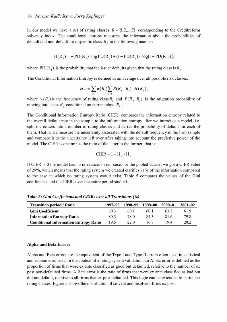
In our model we have a set of rating classes }7,...,2,1{=R corresponding to the Creditreformsolvency index. The conditional entropy measures the information about the probabilities ofdefault and non-default for a specific class jR in the following manner:
[ ]))R(PD1log())R(PD1()R(PDlog)R(PD)R(H jjjjj −⋅−+⋅−= ,
where )R(PD j is the probability that the issuer defaults given that the rating class is jR .
The Conditional Information Entropy is defined as an average over all possible risk classes:
��==
⋅=j
jiji
iC RHRRPRwH11
)()|()( ,
where )( iRw is the frequency of rating class iR and )|( ij RRP is the migration probability ofmoving into class jR conditional on current class iR .
The Conditional Information Entropy Ratio (CIER) compares the information entropy related tothe overall default rate in the sample to the information entropy after we introduce a model, i.e.split the issuers into a number of rating classes and derive the probability of default for each ofthem. That is, we measure the uncertainty associated with the default frequency in the firm sampleand compare it to the uncertainty left over after taking into account the predictive power of themodel. The CIER is one minus the ratio of the latter to the former, that is:
0C H/H1CIER −=
If CIER is 0 the model has no relevance. In our case, for the pooled dataset we got a CIER valueof 29%, which means that the rating system we created clarifies 71% of the information comparedto the case in which no rating system would exist. Table 5 compares the values of the Ginicoefficients and the CIERs over the entire period studied.
Table 5: Gini Coefficients and CEIRs over all Transitions (%)
Transition period / Ratio 1997–98 1998–99 1999–00 2000–01 2001–02Gini Coefficient 60.3 60.1 60.1 63.2 61.9Information Entropy Ratio 80.5 78.0 84.3 81.6 79.8Conditional Information Entropy Ratio 19.5 22.0 16.7 19.4 20.2
Alpha and Beta Errors
Alpha and Beta errors are the equivalent of the Type I and Type II errors often used in statisticaland econometric tests. In the context of a rating system validation, an Alpha error is defined as theproportion of firms that were ex ante classified as good but defaulted, relative to the number of expost non-defaulted firms. A Beta error is the ratio of firms that were ex ante classified as bad butdid not default, relative to all firms that ex post defaulted. This logic can be extended to particularrating classes. Figure 5 shows the distribution of solvent and insolvent firms ex post.

Credit Risk and Bank Lending in the Czech Republic 17
Figure 5: Ex Post Analysis of (In)solvent Enterprises
Figure 6 separates the good firms from the bad ones. It shows that most of the solvent enterprisesbelonged to the positive rating classes while insolvent companies were predominantly in thedefault class. To identify the Alpha and Beta errors in the rating system it is necessary to comparethe number of firms predicted by the model as good (in rating classes 1 to 7) with the real defaultsin the next period. This represents the Alpha Error, which is a measure of the default risk.Analogously, one can consider all enterprises classified as bad by the model and compare them tothe real outcome of defaulted firms. All those who did not default represent the Beta error. TheBeta error is divided over all non-defaulting companies, resulting in a relatively small number,which can be seen in the following figure.
Figure 6: Classification Error over Rating Classes
0%
20%
40%
60%
80%
100%
1 2 3 4 5 6 7 8
solvent insolvent
Beta-Error
Alpha-Error
0%
10%
20%
30%
40%
50%
60%
70%
1 2 3 4 5 6 7 8
solvent insolvent

18 Narcisa Kadlčáková, Joerg Keplinger
Table 6 shows the distribution of Alpha and Beta errors over the entire period. Like the Ginicoefficient it shows the discrimination power of the rating system, which is visualized as the areabetween both figures. The Alpha error for the insolvent companies is around 42%. Thesecompanies were previously rated as good and subsequently defaulted. If they had been givencredit this would have resulted in a loss. The Beta error (0.27%) represents only administrationcosts or lost business, since it refers to those companies which were refused credit in the past butwould have otherwise been creditworthy. The first period 1997/98 cannot be taken into account asit is the first transition period and does not include previous defaults for verification. The Alphaerror is decreasing over time overall, which is positive for identifying default risk.
Table 6: Alpha / Beta Errors over transitions
Transition period Alpha Error Beta Error1998/1999 47.16% 0.27%1999/2000 32.52% 0.25%2000/2001 39.56% 0.22%2001/2002 31.21% 0.40%
In terms of Alpha / Beta errors, our model displayed a slightly higher Alpha error (42% comparedto 39%) and a significantly lower Beta error (0.27% compared to 9%) than in Austria (see Table7). However, this comparison is only a rough benchmark for the quality of our model, since theinput data were slightly different. Not ignoring the fact that the data had a longer history andbetter quality in Austria, we can nevertheless conclude that the rating system built upon the Czechversion of the Creditreform data is close to international standards.
Table 7: Comparison of Creditreform rating system: Czech Republic vs. Austria (%)
Creditreform –rating system
Czech Republic
Creditreform –rating system
Austria
Moody’s – ratingsystem APPLIED
IN AustriaGini Coefficient 63 81 79Information EntropyRatio
79 83 88
4.3 Migration Matrices
The next step is to construct the one-year migration matrices. The elements situated on the rowsof these matrices represent the percentage of firms that, starting from a certain rating class at thebeginning of the period, migrate to another rating class at the end of the one-year period. Theassumption made by the cohort approach is that the historical frequencies of migration are goodapproximations of the implicit migration probabilities. Appendix A1 contains the migrationmatrices associated with our rating system. In general, the probability mass of the migration isconcentrated on the first diagonal, meaning that migrations become less likely as the distancebetween classes becomes higher. Appendix A1 also contains the average of the five migrationmatrices (cell-by-cell average) over the six-year period.

Credit Risk and Bank Lending in the Czech Republic 19
In the literature, rating systems are typically assumed to display Markov (stochastic) properties. Inthis sense the probability distribution R(t) of the credit ratings of an obligor is assumed to follow aMarkov process, i.e. the history of R(t) is described by the relation ( ) ( ) MtR1tR ⋅=+ , where Mis the migration matrix among the rating classes. Under the Markov assumption, migrationmatrices are supposed to be time homogeneous (constant in time). The time homogeneousassumption is an extremely useful property, since, if it holds, it allows the computation of multi-period migration matrices as the power of the one-year migration matrix. The extent to whichmigration matrices satisfy the time homogeneity property in our rating system is evaluated bymeans of several matrix metrics that assess the discrepancy among matrices. These metrics arecalled mobility indices. They have often been referred to in the literature in connection with thetime homogeneity property of the migration matrices of a rating system2.
Given two migration matrices A and B whose elements n,1j,ibanda j,ij,i = sum to one for eachi (stochastic matrices), the following metrics can be computed:
1. ( )( )2
n
1i
n
1jj,ij,i
1
n
baabsB,AL
��= =
−= ,
2. ( )( )
2
n
1i
n
1j
2j,ij,i
2
n
ba
B,AL��= =
−
= ,
3. ( ) ( ) ( )ABB,AE 22 λλ −= , where ( )⋅2λ is the largest eigenvalue below one,
4. ( )( ) ( )
n
B~B~
n
A~A~
B,AJS
n
1ii
n
1ii ��
==
′−
′=
λλ.
The first two metrics are the equivalent of the standard Euclidian distances defined in the nRspace. They aggregate into an overall measure the cell-by-cell distances between the elements ofthe two matrices. The third measure captures differences in the convergence rates towards thesteady states of the probability distributions R governed by the two transition matrices. The fourthmeasure reflects differences in the average probability of migration as defined by Jafry andSchuermann (2003). Their matrix norm is constructed as the average of the singular values of themobility matrix A~A~ ′ ( )A~(transposeA~,IAA~ =′−= , A = the migration matrix, I = the identitymatrix of order n). The singular values represent the square root of the eigenvalues of the matrix
A~A~ ′ . This norm describes an “average” propensity of migration of the rating system from thecurrent rating classes to different rating classes within the considered period. The closer to zerothese metrics are, the more likely it is that the time homogeneity assumption is valid.
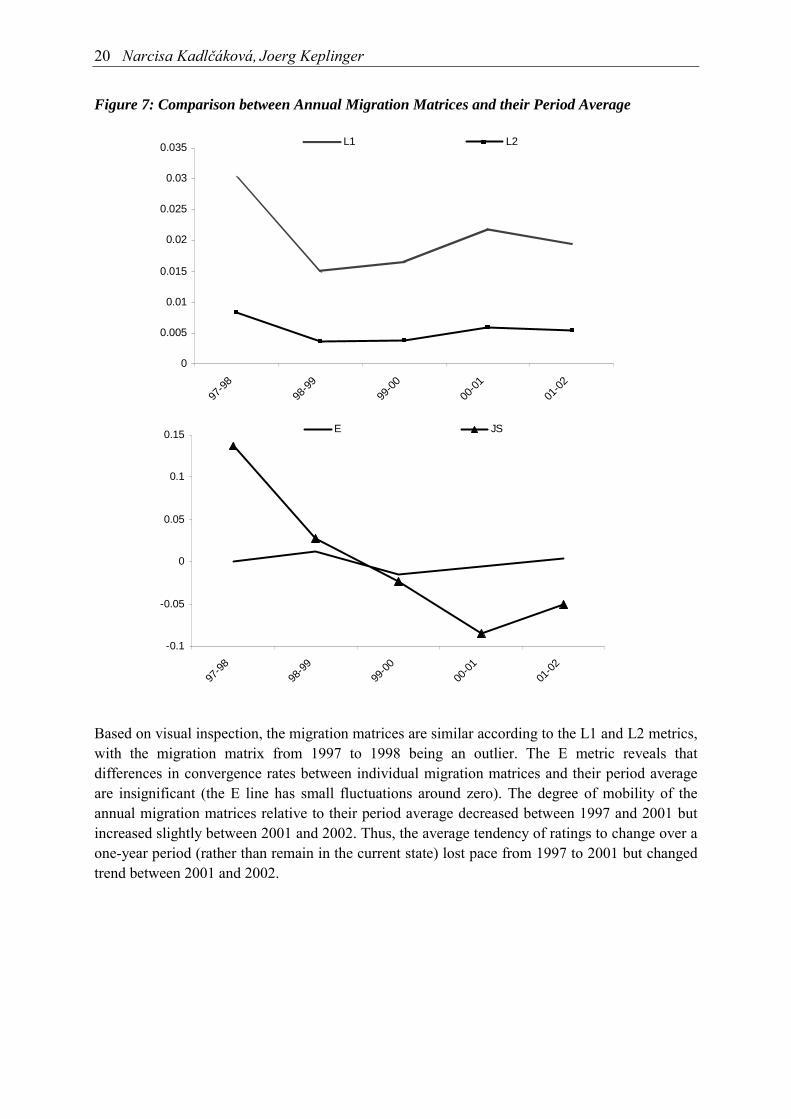
Computing the values of these metrics it is possible to compare the “distance” between annualmigration matrices and their period average. Figure 7 depicts the results.
2 However, to our knowledge these mobility indices do not constitute a formal test statistic by themselves.Further research in this direction is required.
20 Narcisa Kadlčáková, Joerg Keplinger
-0.1
-0.05
0
0.05
0.1
0.15
97-98
98-99
99-00
00-01
01-02
E JS
Figure 7: Comparison between Annual Migration Matrices and their Period Average
Based on visual inspection, the migration matrices are similar according to the L1 and L2 metrics,with the migration matrix from 1997 to 1998 being an outlier. The E metric reveals thatdifferences in convergence rates between individual migration matrices and their period averageare insignificant (the E line has small fluctuations around zero). The degree of mobility of theannual migration matrices relative to their period average decreased between 1997 and 2001 butincreased slightly between 2001 and 2002. Thus, the average tendency of ratings to change over aone-year period (rather than remain in the current state) lost pace from 1997 to 2001 but changedtrend between 2001 and 2002.
0
0.005
0.01
0.015
0.02
0.025
0.03
0.035
97-98
98-99
99-00
00-01
01-02
L1 L2

Credit Risk and Bank Lending in the Czech Republic 21
5. Credit Risk Modeling for Czech Loans
5.1 Introduction to Credit Risk Modeling
The release of a series of consultative documents and quantitative impact studies by the BaselCommittee and several commercial credit risk models by renowned financial institutions hasreinforced the awareness of the banking sector of the necessity to measure and control the riskassociated with banks’ lending operations. The publication in 2001 of the New Basel CapitalAccord and three consequent impact studies triggered an intensive dialog among regulators andbankers worldwide. The aim is to formulate an optimal set of norms and regulations meant tobecome standard practice in bank capital provisioning against credit risk by 2006. At the sametime, credit risk models have raised constant interest within the banking industry because thesemodels allow sensitive measurement of default risk at the portfolio level. The most prominentcredit risk models developed and to a certain extent already applied by the banking industry areCredit Metrics (JP Morgan), CreditRisk+ (Credit Suisse Financial Products), KMV (Moody’s –KMV) and CreditPortfolioView (McKinsey’s & Company).
In what follows, the methodologies applied in this paper are briefly presented: the Internal RatingsBased (IRB) approach as formulated by the latest Consultative Document of the NBCA (April2003), and the Credit Metrics and CreditRisk+ models. The main goal of the paper is to reflect onthe applicability of these methodologies and not to offer a comprehensive theoretical description.For this reason the remaining part of this section sketches the most important steps that areessential in estimating the risk capital in each considered case.
5.1.1 The New Basel Capital Accord (NBCA)
The regulatory guidelines referring to credit risk assessment and capital budgeting are exposed inthe NBCA under two main headings, the standardized approach and the Internal Ratings Based(IRB) approach. Irrespective of the approach selected, banks are supposed to categorize all theirexposures within a well-defined range of categories and to apply category-specific regulatoryrules3. The contribution of credit risk-related regulatory capital to an overall minimum capitalrequirement (additionally incorporating capital for market and operational risk) is identical underthe two approaches.
The standardized approach relies on rating systems provided by external agencies (Moody’s –KMV, S&P) and on risk weights that are calibrated to the rating classes of these rating systems.The IRB approach specifies concrete regulatory capital formulas permitting banks to use theirown estimations of the required input data, including among them banks’ internal ratings. If abank applies the IRB approach, it has to estimate the following risk inputs at the obligor (asset)level: the probability of default (PD), an estimate of the loss incurred if default occurs (Loss
3 The following claim categories are considered under the standardized approach: sovereigns, non-centralgovernment public sector entities (PSEs), multilateral development banks, banks, securities firms and corporates.Considered under the IRB approach are sovereign, bank, corporate, retail, equity and purchased receivablesexposures.

22 Narcisa Kadlčáková, Joerg Keplinger
Given Default or LGD), the loan exposure (EAD) and an effective maturity (M). Specificeligibility criteria are provided in the regulatory documents that allow banks to estimate these riskinputs based on an internal process. Additionally, under the IRB approach two alternativeprocedures are mentioned, the foundation approach and the advanced approach. Under thefoundation approach, banks may derive their own estimates only for the PDs4, with all other risk-input estimations conforming to the regulatory rules. Under the advanced approach, banks can usetheir own estimates for all the required risk inputs.
The initial IRB methodology for corporate exposure (January 2001) was significantly modified inthe recent Consultative Document of the NBCA (April 2003). The current formulation entails theapplication of the following algorithm when computing a risk-adjusted value of a bank asset:
• Computing a correlation coefficient (R):
( ) ( )
���
�
���
�
−−−⋅+
−−⋅=
−
+−
−
+−
50
PD50
50
PD50
e1e11240
e1e1120R .. ,
• Computing a maturity adjustment coefficient (b):
( )2058980084510b ln(PD)⋅−= .. ,
• Computing a capital requirement coefficient (K)5:
( ) ( ) ( ) ( )( )PDb511
PDb52M19990GR1
RR1
PDGNLGDK⋅−
⋅−++��
���
�⋅
−+
−⋅=
... ,
• Estimating the risk-weighted asset value:
EADK512RW ⋅⋅= . .
The regulatory capital represents 8% of the sum of the risk-weighted assets. Our computationsconformed to the foundation approach of the IRB by employing our own estimates for the PDsand determining all other risk inputs according to the regulatory rules. We used an LGD value of45% (as required for senior claims on corporates), an effective maturity of 2.5 years and an EADequal to the face value of the loans (the amount legally owed to the bank).
4 The only restriction that applies in this case is that the PDs are bounded from below by the 0.03% value,meaning that PDs below this value (according to the bank’s internal rating system) must be replaced by the0.03% value for regulatory capital estimation purposes.5 N(x) and G(x) denote the cumulative distribution function for a standard normal distribution and its inverse,respectively. It should also be mentioned that the PD value must be expressed as whole numbers in thecomputation of R. For example, a PD of 2.5% should enter the R formula as 2.5 and not as 0.025. On thecontrary, in computing the coefficients b and K one must use PD values in the traditional sense, thus as numbersbetween 0 and 1.
Credit Risk and Bank Lending in the Czech Republic 23
5.1.2 CreditMetrics
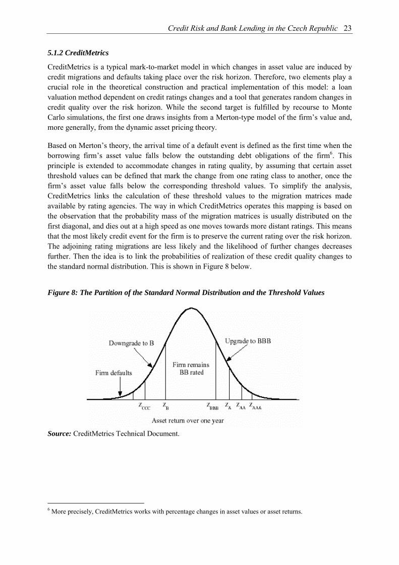
CreditMetrics is a typical mark-to-market model in which changes in asset value are induced bycredit migrations and defaults taking place over the risk horizon. Therefore, two elements play acrucial role in the theoretical construction and practical implementation of this model: a loanvaluation method dependent on credit ratings changes and a tool that generates random changes incredit quality over the risk horizon. While the second target is fulfilled by recourse to MonteCarlo simulations, the first one draws insights from a Merton-type model of the firm’s value and,more generally, from the dynamic asset pricing theory.
Based on Merton’s theory, the arrival time of a default event is defined as the first time when theborrowing firm’s asset value falls below the outstanding debt obligations of the firm6. Thisprinciple is extended to accommodate changes in rating quality, by assuming that certain assetthreshold values can be defined that mark the change from one rating class to another, once thefirm’s asset value falls below the corresponding threshold values. To simplify the analysis,CreditMetrics links the calculation of these threshold values to the migration matrices madeavailable by rating agencies. The way in which CreditMetrics operates this mapping is based onthe observation that the probability mass of the migration matrices is usually distributed on thefirst diagonal, and dies out at a high speed as one moves towards more distant ratings. This meansthat the most likely credit event for the firm is to preserve the current rating over the risk horizon.The adjoining rating migrations are less likely and the likelihood of further changes decreasesfurther. Then the idea is to link the probabilities of realization of these credit quality changes tothe standard normal distribution. This is shown in Figure 8 below.
Figure 8: The Partition of the Standard Normal Distribution and the Threshold Values
Source: CreditMetrics Technical Document.
6 More precisely, CreditMetrics works with percentage changes in asset values or asset returns.

24 Narcisa Kadlčáková, Joerg Keplinger
The figure shows the partition of the region under the standard normal distribution in distinctzones, whose areas equal the migration probabilities of the BBB rating class according to the S&Prating system. The middle zone characterized by the largest area reflects the probability ofpreserving the BBB rating. The next step is to observe that these zones are well delimited and canbe mapped in a one-to-one manner into a set of real numbers (the Z values on the x axis on thefigure). These Z values are called threshold values and are computed with the help of the inverseof the standard normal cumulative function.
The calculation of the threshold values represents the key tool in implementing Monte Carlosimulations. The idea is to draw random numbers from the standard normal distribution (one foreach asset), to compare them with the rating class-specific threshold values and to assess whatrating migrations these numbers would suggest. This procedure is complicated to some extent inthe portfolio context, since rating migrations for different obligors are, as a rule, correlated.Performing independent random draws from the normal distribution would make no sense in thiscontext. The problem, however, can be easily solved on the basis of Cholesky factorization orsingular value decomposition methods that are usually available in the current statistical softwareprograms.
An important aspect of the CreditMetrics model is the loan valuation. Depending on the creditmigration occurring in the case of non-default, a loan can be valued according to the formula:
( ) ( ) ,d1
Fr
d1
rV1T
1tTg
Ttg
t
gg
i
i
i
�−
= ′′′
+
+++
= (1)
where r and F are the loan interest and face value, and dtg′ are the discount factors for the years 1
to T, applicable to the rating class g' (here T is the maturity of the loan). In this specification it isassumed that the present rating changes from g to g' over the one-year period. In the case ofdefault the present value of the loan is computed as the product of the face value of the loan andthe recovery rate. The portfolio value is the sum of the individual loans’ valuations.
A particular difficulty in (1) is posed by the estimation of the discount factors d entering bankloans’ valuation. This estimation relies on risk neutral probabilities whose existence (anduniqueness) is conditional on the assumption of complete markets and no-arbitrage conditions.Even if these general assumptions are disregarded in practice, the estimation of the discountfactors is still problematic, since it requires information on the price of risk in the loan market.Since loans are non-traded debt instruments, the price of risk can be at most proxied. At least froma theoretical point of view, a few approaches for the estimation of the discount factors have beendeveloped, one of which will be explained in more detail in Subsection 5.2.
Random draws of real numbers replicate random changes in credit quality. Contingent on therating migration simulated, loans are re-evaluated and the portfolio value is computed. This is theprinciple of the Monte Carlo simulation. Random drawings of real numbers are performed a largenumber of times (preferably ten thousand times or more). The corresponding portfolio valuesgenerate the empirical portfolio distribution. Economic capital estimations can then be performedin a manner to be presented in Subsection 5.3.

Credit Risk and Bank Lending in the Czech Republic 25
5.1.3 Credit Risk+
CreditRisk+ is a default mode model that borrows intensively from the actuarial models used ininsurance economics. Default mode means that the credit standing of a certain obligor over therisk horizon can reach only two states: default and non-default. CreditRisk+ adopted the reduced-form approach to modeling default risk by calibrating random default and loss events to standardstatistical distributions. Even if default events at the individual obligor level are not directlymodeled, default probabilities represent a compulsory input into the CreditRisk+ model and mustbe estimated by the credit analyst.
The approach followed by CreditRisk+ is to “homogenize” the pool of risky loans by groupingthem into classes (“bands” in the CreditRisk+ terminology) with similar risk characteristics. Thedeciding factor in performing this classification is the so-called common exposure at the bandlevel. In this sense, credit exposures are scaled down by a selected unit of exposure and obligorswith similar exposures (after rescaling and rounding to the nearest integer) are grouped together.Two distributions are relevant in the analysis. The distribution of default events at the band levelis modeled as a Poisson distribution:
( )!kemkdefaultsofnumberP
mk −
== , k = 1, 2,...
with the expected number of defaults given by m and with a standard deviation m . The seconddistribution is the one related to the entire portfolio loss, i.e. portfolio losses expressed asmultiples of the unit of exposure related to their probabilities of realization. The derivation of bothdistributions rests upon the construction of a probability generating function and its statisticalproperties. In the latter case a recursive formula is derived that estimates the probabilities that lossequals multiples of the unit of exposure. The estimation of the economic capital is performed onthe basis of the portfolio loss distribution thus derived in a manner to be presented in Subsection5.3.
CreditRisk+ allows two types of generalizations in the basic set-up, a risk analysis extending overa multi-year period and a risk analysis with variable default rates. In the latter case diversificationeffects are captured in the model by incorporating the sensitivity of the obligors to systemic riskfactors (“sectors” in the CreditRisk+ terminology). The average default rate of a certain sector isassumed to follow a Gamma distribution, which transforms the random variable describing thenumber of defaults at the sector level into a negative binomial distribution. The same reasoning asin the basic case applies for the derivation of the portfolio loss distribution in this case.
We applied the CreditRisk+ model with a multi-year default structure and with all the exposuresassigned to a single sector (the general economy). Default rates at horizons longer than one yearwere determined by multiplying the one-year migration matrix by itself n times (n is the numberof years) and then examining the elements situated in the last column of the resulting matrices.

26 Narcisa Kadlčáková, Joerg Keplinger
5.1.4 The Czech Loan Portfolio
The Czech economy has undergone dramatic changes and dynamic development since the 1989revolution. The corporate sector is now mostly privatized and Czech banks are currently mainlyforeign-owned. The banking system has stabilized after a series of bank bankruptcies that tookplace at the beginning of the transition period. However, even if default rates have beendecreasing for years, credit risk still represents a major risk for bank lending operations tobusinesses. Classified loans (for which payment has been delayed for more than 30 days) as apercentage of the total credit volume fell from 32% in 1999 to 16% in 2002.
In what follows we construct a representative portfolio for bank lending to corporates in theCzech Republic. The assets of the portfolio are represented by bank credits to Czech industries(according to the NACE classification). For this reason the terms assets and industries will beused interchangeably in the rest of the paper. In principle, defining the portfolio is tantamount toestimating all the industry characteristics that represent the necessary inputs in the different creditrisk methodologies approached in this paper. A quick reference to the required input data iscontained in Table 8.
Table 8: Input Data Required by Different Approaches
NBCA CREDITMETRICS CREDITRISK+• Ratings and PDs• Credit exposures• Maturities• Recovery rates
• ratings and PDs/migration matrices• credit exposures• maturities• recovery rates• interest rates on loans• asset return correlations• discount factors (credit spreads)
• credit exposures• PDs• PDs’ volatilities
The remaining part of this section examines our data sources and the methodologies applied toestimate the required model inputs.
5.1.5 Ratings
To assign ratings at the industry level we computed historical default rate frequencies and theirperiod averages at each industry level. The statistical significance of the average default rates wasassessed according to the methodology proposed by Cantor and Falkenstein (2001). Moreprecisely, following their notation let us define:
• t,in as the number of firms in industry i at time t,
• t,id as the number of defaults in industry i at time t,
• tiPD , as the default rate in industry i at time t,
• �=t
t,ii nN as the number of issuer-years in industry i,
• �=t
t,ii dD as the number of defaults-years in industry i,
• i
ii N
DPD = as the average default rate over the entire period in industry i.

Credit Risk and Bank Lending in the Czech Republic 27
Assuming that the underlying (true) default rate ip of industry i is constant in time, Cantor andFalkenstein show that the empirical default rates tiPD , and iPD are approximately normally
distributed with mean ip and standard deviations ( )
t,i
ii
np1p −⋅
and ( )
i
ii
Np1p −⋅
, respectively.
If the underlying default rate is not constant in time, due either to fluctuating macroeconomicconditions or to idiosyncratic reasons at the industry level, then the average default rate for
industry i has a standard deviation of ( )
�+−⋅
t
2t,i2
i
2
i
ii nNN
p1p σ, where σ is the standard
deviation of a macroeconomic shock affecting the economy.
Standard deviations at the industry level were computed assuming both constant and variable truedefault rates. In the latter case σ was approximated by the standard deviation of the default rateof the entire sample of firms over the period 1997–2002. In the final portfolio we selected thoseindustries that displayed standard deviations of the default probabilities of less than 2%.Additionally, we eliminated those industries for which the sample contained a very small numberof firms.
The results are reported in Appendix A2. The elements of that table contain annual default rates atthe industry level, the standard deviations of the average default rates and the rating classassignment of each industry. Designated in bold numbers are the industries whose average defaultrates seemed reliable and thus were considered as assets of the portfolio. By comparing the defaultrates at the industry level (the average) with the default rates situated in the last column of theaverage transition matrix, we assigned the individual industries to rating classes. For example, ifthe average PD of a given industry was 4.14% (agriculture), the industry was assigned to therating class 5, since its PD belonged to the interval defined by the representative PDs of the fourthand fifth classes.
5.1.6 Credit Exposure
We aggregated the loan volumes granted by all Czech banks to non-financial firms. These loansare reported as a stock at the end of each month in the SUD database of the Czech National Bank.We sorted the loans according to industry destination, currency denomination (Czech crowns, USdollars and euro) and the maturity classification used by the Czech National Bank (less than 1year, 1–4 years, 4–5 years, more than 5 years). We aggregated only loan volumes in theclassification range from one to four, with non-performing loans (loss loans or loans in the fifthcategory) being neglected. The aggregate bank credit exposure respecting this structure wasestimated at the end of 2002 and is shown in Appendix A3.
5.1.7 Interest Rates
Loan interest rates are not classified according to industry in the databases of the Czech NationalBank. For this reason we used data made available by the Ministry of Industry and Trade of theCzech Republic. We computed an implicit interest rate at the NACE level defined as the ratiobetween interest expenditure and total bank loans at the industry level at the end of 2002.

28 Narcisa Kadlčáková, Joerg Keplinger
Unfortunately, these estimations provided only a general indication of the loan interest rates andwere not differentiated according to loan maturity. For those industries for which relevant datawas missing we used the figures available at the next level of aggregation (for example, data wasavailable as an aggregate over NACE 50, 51 and 52 but not at the level of each of these industries)or the economy-wide average (NACE 1). The results are displayed in Appendix A4.
5.1.8 Recovery Rates
No explicit measure of the loans’ recovery rates at the industry level is publicly available. For thisreason we assumed a recovery rate of 55% for all industries. This figure is compatible with the45% LGD value considered in the regulatory case7.
5.1.9 Asset Return Correlations
Asset returns at the industry level were proxied by the corresponding producer price indices andcorrelations among these indices were computed. The implicit assumption made was that anadverse shock affecting a certain industry would induce a fall in the corresponding producerprices. In principle, measuring correlations among sectoral equity returns would have beenpreferable, since equity indices offer a better image of the trends in asset returns at the industrylevel. The main drawback was that equity indices were not available for some of the industriesincluded in the portfolio. Additionally, the feeble firm representation on the Czech StockExchange could have depicted a biased picture of the real productivity trends of particularindustries anyway.
Each price index was divided by the PPI to eliminate systemic influences that could have inflatedthe correlations. Monthly price indices that covered the period January 1995 – September 2003were obtained from the Czech Statistical Office. Since such price indices were not available forthe industries NACE 52, 63 and 73 these industries were not further considered. The industriesNACE 65 and 67 represented the financial sector, so they were also ignored in the computations.Correlations among price indices at the industry level are contained in Appendix A5.
5.1.9 Discount Factors (Credit Risk Spreads)
The approach of Jarrow, Lando and Turnbull was implemented to estimate the term structure ofcredit spreads. Jarrow, Lando and Turnbull formalize changes in rating quality as a Markov chaindescribed by a time-homogeneous migration matrix.
Consider an n-class rating system }D,...,2,1{R = (the last class D denoting default) and the
associated time homogeneous migration matrix M whose elements ijM represent the probability
of migration between the rating classes i and j. If the life horizon of the loan [0, T] is divided intom intervals [t, t+1], t = 0,…,T-1 over which changes in credit quality may occur, the risk premia at
7 The recovery rate is 1-LGD.

Credit Risk and Bank Lending in the Czech Republic 29
time t are the rescaling factors ( )tiπ that transform the physical migration probabilities ijM into
the corresponding risk-neutral migration probabilities ( )1t,tMij +∗ :
( ) ( ) ijiij Mt1t,tM ⋅=+∗ π , i, j = 1,n, i = j
In Jarrow, Lando and Turnbull the estimation of the risk premia is done recursively. The spotvalues ( )0iπ are given by
( ) ( ) ( )( ) ( ) iD
0
0
i M11,0B1,0B1,0B0
⋅δ−⋅−=π
where ( )1,0B0 and ( )1,0Bi are the “prices” of default-free and risky loans respectively, δ is therecovery rate and iDM is the default rate of the rating class i. At the time horizon t the risk premiavalues are the solution of the system
( )( )
( )
( ) ( )( )( )
( ) ( )( )( ) �
�����
�
�
������
�
�
−++−+
−++−+
=���
�
�
���
�
�
⋅
⋅⋅∗
δ
δ
π
π
11,01,01,0
.....11,0
1,01,0
.....,0
0
0
01
0
11
tBtBtB
tBtBtB
Mt
MttM
DDDD
D
(2)
where ( )t,0M∗ is the risk neutral migration matrix between time 0 and t defined by the recursive
formula ( ) ( ) ( ) ( )[ ]IM1tI1t,0Mt,0M −⋅−π+⋅−= ∗∗ .
Jarrow, Lando and Turnbull also derive a closed form solution for the credit spreads
( ) ( ) ( ) iDii Mt11
1lntS⋅π⋅δ−−
= . (3)
In our case the “prices” of default free and risky loans in (2) were computed as
( ) ( ) t)r(i
tr0 ittt et,0Bandet,0B ⋅+−⋅− == ϕ , t = 1, 2,…,6
where tr was the risk free rate (1-year PRIBOR) and itϕ were the interest rate charges on riskyloans requested by some Czech banks at the end of 2002. Here t represents the maturity of theloans and i the rating class.
The credit spread estimations in the Czech market based on (3) are depicted graphically inAppendix A6
The Jarrow, Lando and Turnbull model constitutes a convenient theoretical technique for theestimation of the credit spreads in the Czech bank loan market. The main deficiency of thisestimation was related to the quality of the input data. The interest rate charges on risky loanswere calibrated to banks’ internal rating systems and these rating systems were not consistent withthe one we used. Moreover, the probabilities of default characterizing our risky classes (the sixth

30 Narcisa Kadlčáková, Joerg Keplinger
and seventh classes) were significantly higher than the default probabilities accepted by the Czechbanks when granting loans to corporate clients. Since interest charges on loans with such riskcharacteristics were not available as real data we had had to perform several calibrations8.Additionally, since data was obtained from a small number of banks, the possibly of depicting abiased picture is very high.
The estimated model inputs are summarized in Table 9. This represents the 33-asset portfolio onwhich the aforementioned methodologies were applied.
Table 9: Czech Loans Portfolio
NACE AverageDefault
Rate
RatingClass
LoanExposure(bil. CZK)
ImplicitLoan
Interest Rate
Maturity(years)
RecoveryRate
1 – Agriculture 4.14% 5 14.76 16.30% 6 55%14 – Mining other 2.86% 4 1.47 6.23% 6 55%15 – Manufacture of food products and
beverages7.51% 6 22.24 8.65% 6 55%
17 – Manufacture of textiles 4.22% 5 6.37 9.27% 6 55%18 – Manufacture of wearing apparel;
dressing and dyeing of fur4.11% 5 2.49 11.88% 6 55%
20 – Manufacture of wood and ofproducts of wood
7.73% 6 2.05 7.76% 6 55%
21 – Manufacture of pulp, paper andpaper products
3.56% 4 7.03 6.79% 6 55%
22 – Publishing, printing and reproductionof recorded media
4.17% 5 4.59 7.81% 6 55%
24 – Manufacture of chemicals andchemical products
2.98% 4 14.15 9.18% 6 55%
25 – Manufacture of rubber and plasticproducts
3.39% 4 7.88 9.90% 6 55%
26 – Manufacture of other non-metallicmineral products
4.90% 5 14.14 11.49% 6 55%
27 – Manufacture of basic metals 6.07% 6 5.49 10.29% 6 55%28 – Manufacture of fabricated metal
products4.36% 5 8.21 12.63% 6 55%
29 – Manufacture of machinery andequipment
4.72% 5 12.92 11.14% 6 55%
30 – Manufacture of office machinery andcomputers
5.41% 6 0.17 1.66% 6 55%
31 – Manufacture of electrical machineryand apparatus
2.59% 3 5.67 15.56% 6 55%
32 – Manufacture of radio, television andcommunication equipment andapparatus
3.49% 4 0.82 19.12% 6 55%
8 More precisely, for the last two rating classes (associated with default probability values of 10% and 20%) weassumed interest rate charges over the risk free rate of 50% and 200%, respectively. This was an artificial way toreflect the fact that Czech banks refuse, as a rule, to grant loans to corporate customers with default probabilitiesin this range. However, these assumptions affected the estimation of the credit spreads in the last two non-defaulted classes. Since credit risk spreads are essential for CreditMetrics, its estimated economic capital valuesare to some extent inadequate.

Credit Risk and Bank Lending in the Czech Republic 31
33 – Manufacture of medical, precisionand optical instruments, watches andclocks
3.65% 4 1.19 8.80% 6 55%
34 – Manufacture of motor vehicles,trailers and semitrailers
1.29% 2 7.33 28.29% 6 55%
36 – Manufacture of furniture 5.12% 6 4.63 7.87% 6 55%37 – Recycling 3.37% 4 0.64 14.73% 6 55%40 – Electricity, gas, steam and hot water
supply2.80% 4 24.90 13.96% 6 55%
41 – Collection, purification anddistribution of water
0.00% 1 2.75 3.06% 6 55%
45 – Construction 5.58% 6 9.81 9.83% 6 55%50 – Sale and repair of motor vehicles and
cycles and fuel4.45% 5 9.58 9.63% 6 55%
51– Wholesale trade 5.70% 6 56.53 9.63% 6 55%55 – Hotels and restaurants 5.79% 6 2.21 7.03% 6 55%60 – Land transport; transport via
pipelines2.39% 3 16.44 16.30% 6 55%
64 – Post and telecommunications 1.89% 3 10.67 16.30% 6 55%70 – Real estate 8.99% 6 36.69 11.05% 6 55%71 – Renting of machinery and equipment 4.80% 5 13.01 11.05% 6 55%72 – Computer and related activities 1.45% 3 3.04 11.05% 6 55%74 – Other business activities 5.59% 6 21.47 11.05% 6 55%
5.2 Regulatory and Economic Capital Estimations
Table 10 illustrates the algorithm discussed in 5.1.1 for the estimation of regulatory capital.
Table 10: Regulatory Capital According to the IRB Approach
NACE PD EXPOSURE(bil.CZK)
R B K RWA(bil.CZK)
1 4.14% 14.76 0.12 0.07 0.12 22.3714 2.86% 1.47 0.12 0.09 0.10 1.7915 7.51% 22.24 0.12 0.06 0.17 47.4517 4.22% 6.37 0.12 0.07 0.12 9.7618 4.11% 2.49 0.12 0.07 0.12 3.7520 7.73% 2.05 0.12 0.06 0.17 4.4521 3.56% 7.03 0.12 0.08 0.11 9.7422 4.17% 4.59 0.12 0.07 0.12 6.9924 2.98% 14.15 0.12 0.09 0.10 17.6125 3.39% 7.89 0.12 0.08 0.11 10.6126 4.90% 14.14 0.12 0.07 0.13 23.6627 6.07% 5.49 0.12 0.06 0.15 10.3928 4.36% 8.21 0.12 0.07 0.13 12.8329 4.72% 12.92 0.12 0.07 0.13 21.1530 5.41% 0.17 0.12 0.07 0.14 0.3031 2.59% 5.67 0.12 0.09 0.09 6.4732 3.49% 0.82 0.12 0.08 0.11 1.1233 3.65% 1.19 0.12 0.08 0.11 1.67
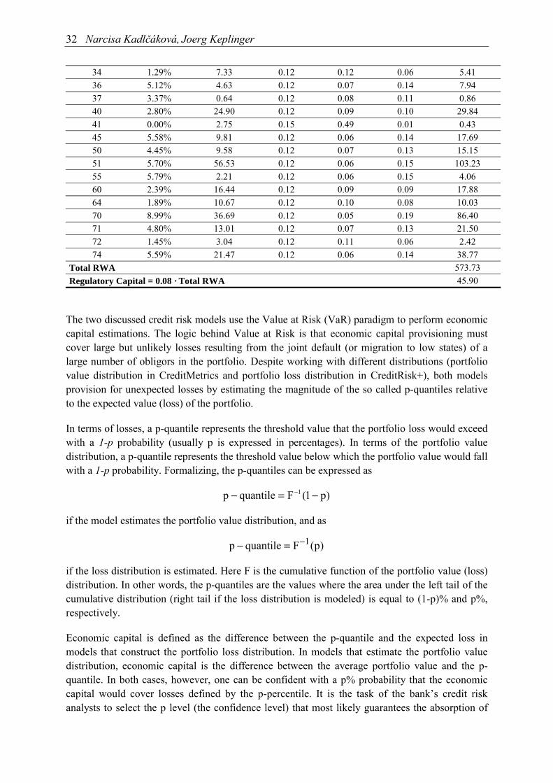
32 Narcisa Kadlčáková, Joerg Keplinger
34 1.29% 7.33 0.12 0.12 0.06 5.4136 5.12% 4.63 0.12 0.07 0.14 7.9437 3.37% 0.64 0.12 0.08 0.11 0.8640 2.80% 24.90 0.12 0.09 0.10 29.8441 0.00% 2.75 0.15 0.49 0.01 0.4345 5.58% 9.81 0.12 0.06 0.14 17.6950 4.45% 9.58 0.12 0.07 0.13 15.1551 5.70% 56.53 0.12 0.06 0.15 103.2355 5.79% 2.21 0.12 0.06 0.15 4.0660 2.39% 16.44 0.12 0.09 0.09 17.8864 1.89% 10.67 0.12 0.10 0.08 10.0370 8.99% 36.69 0.12 0.05 0.19 86.4071 4.80% 13.01 0.12 0.07 0.13 21.5072 1.45% 3.04 0.12 0.11 0.06 2.4274 5.59% 21.47 0.12 0.06 0.14 38.77
Total RWA 573.73Regulatory Capital = 0.08 · Total RWA 45.90
The two discussed credit risk models use the Value at Risk (VaR) paradigm to perform economiccapital estimations. The logic behind Value at Risk is that economic capital provisioning mustcover large but unlikely losses resulting from the joint default (or migration to low states) of alarge number of obligors in the portfolio. Despite working with different distributions (portfoliovalue distribution in CreditMetrics and portfolio loss distribution in CreditRisk+), both modelsprovision for unexpected losses by estimating the magnitude of the so called p-quantiles relativeto the expected value (loss) of the portfolio.
In terms of losses, a p-quantile represents the threshold value that the portfolio loss would exceedwith a 1-p probability (usually p is expressed in percentages). In terms of the portfolio valuedistribution, a p-quantile represents the threshold value below which the portfolio value would fallwith a 1-p probability. Formalizing, the p-quantiles can be expressed as
)p1(Fquantilep 1 −=− −
if the model estimates the portfolio value distribution, and as
)p(Fquantilep 1−=−
if the loss distribution is estimated. Here F is the cumulative function of the portfolio value (loss)distribution. In other words, the p-quantiles are the values where the area under the left tail of thecumulative distribution (right tail if the loss distribution is modeled) is equal to (1-p)% and p%,respectively.
Economic capital is defined as the difference between the p-quantile and the expected loss inmodels that construct the portfolio loss distribution. In models that estimate the portfolio valuedistribution, economic capital is the difference between the average portfolio value and the p-quantile. In both cases, however, one can be confident with a p% probability that the economiccapital would cover losses defined by the p-percentile. It is the task of the bank’s credit riskanalysts to select the p level (the confidence level) that most likely guarantees the absorption of

Credit Risk and Bank Lending in the Czech Republic 33
0
0.00
0.00
0.00
0.00
0.00
0.00
0.00
0.00
0.00
0.0
0 2 4 6 8 10 12 14
Portfolio Loss(CZK bil.)
Frequency
Average Loss
57.
95%-percentile
Economic capital at95% confidence level
102.7
large losses by the maintained capital. The common practice is to focus on values ranging from95% to 99.9%. As a rule, banks might give preference to the 95% value, while the 99% and highervalues represent the more conservative regulatory option.
The two distributions generated by the two credit risk models in our case are depicted in Figures 9and 10.
Figure 9: Portfolio Value Distribution According to the CreditMetrics Model
Figure 10: Portfolio Loss Distribution According to the CreditRisk+ Model
0
0.1
0.2
0.3
0.4
260 280 300 320 340 360
Average Portfolio Value
337
Frequency
Portfolio Value(CZK bil.)
306
95%-percentile Economic capital at95% confidence
level
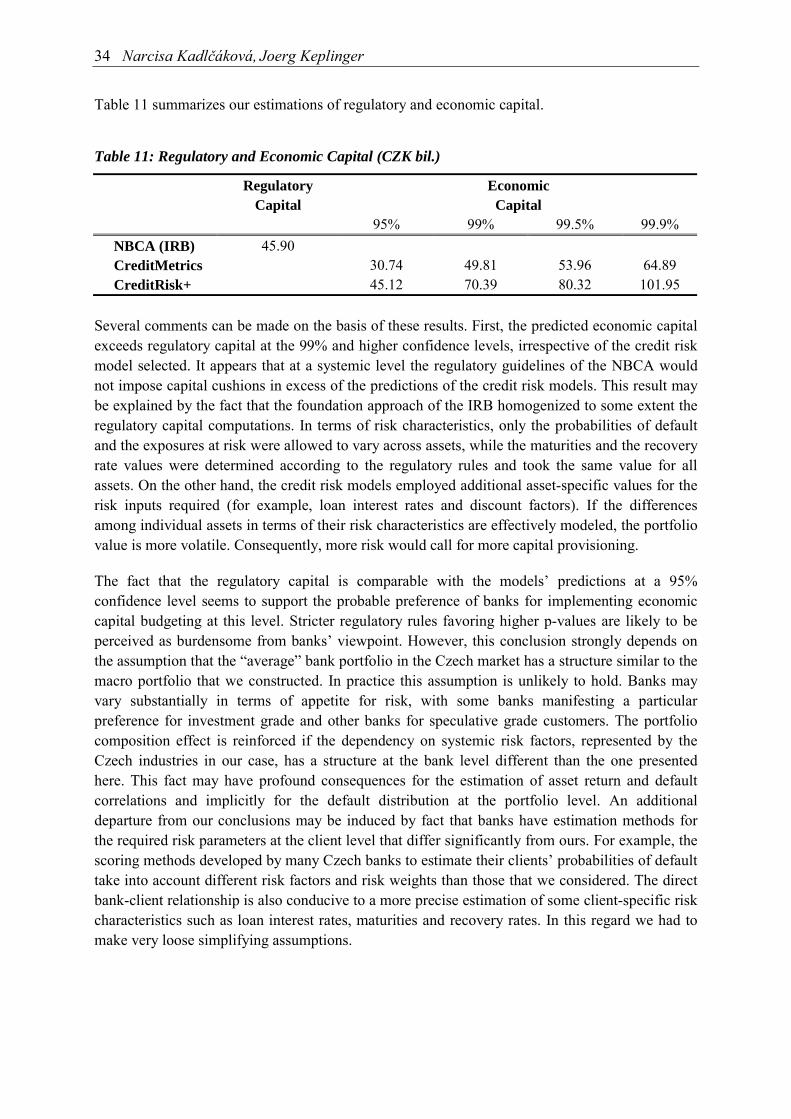
34 Narcisa Kadlčáková, Joerg Keplinger
Table 11 summarizes our estimations of regulatory and economic capital.
Table 11: Regulatory and Economic Capital (CZK bil.)
RegulatoryCapital
EconomicCapital
95% 99% 99.5% 99.9%NBCA (IRB) 45.90CreditMetrics 30.74 49.81 53.96 64.89CreditRisk+ 45.12 70.39 80.32 101.95
Several comments can be made on the basis of these results. First, the predicted economic capitalexceeds regulatory capital at the 99% and higher confidence levels, irrespective of the credit riskmodel selected. It appears that at a systemic level the regulatory guidelines of the NBCA wouldnot impose capital cushions in excess of the predictions of the credit risk models. This result maybe explained by the fact that the foundation approach of the IRB homogenized to some extent theregulatory capital computations. In terms of risk characteristics, only the probabilities of defaultand the exposures at risk were allowed to vary across assets, while the maturities and the recoveryrate values were determined according to the regulatory rules and took the same value for allassets. On the other hand, the credit risk models employed additional asset-specific values for therisk inputs required (for example, loan interest rates and discount factors). If the differencesamong individual assets in terms of their risk characteristics are effectively modeled, the portfoliovalue is more volatile. Consequently, more risk would call for more capital provisioning.
The fact that the regulatory capital is comparable with the models’ predictions at a 95%confidence level seems to support the probable preference of banks for implementing economiccapital budgeting at this level. Stricter regulatory rules favoring higher p-values are likely to beperceived as burdensome from banks’ viewpoint. However, this conclusion strongly depends onthe assumption that the “average” bank portfolio in the Czech market has a structure similar to themacro portfolio that we constructed. In practice this assumption is unlikely to hold. Banks mayvary substantially in terms of appetite for risk, with some banks manifesting a particularpreference for investment grade and other banks for speculative grade customers. The portfoliocomposition effect is reinforced if the dependency on systemic risk factors, represented by theCzech industries in our case, has a structure at the bank level different than the one presentedhere. This fact may have profound consequences for the estimation of asset return and defaultcorrelations and implicitly for the default distribution at the portfolio level. An additionaldeparture from our conclusions may be induced by fact that banks have estimation methods forthe required risk parameters at the client level that differ significantly from ours. For example, thescoring methods developed by many Czech banks to estimate their clients’ probabilities of defaulttake into account different risk factors and risk weights than those that we considered. The directbank-client relationship is also conducive to a more precise estimation of some client-specific riskcharacteristics such as loan interest rates, maturities and recovery rates. In this regard we had tomake very loose simplifying assumptions.
Credit Risk and Bank Lending in the Czech Republic 35
Finally, the different credit risk models’ estimations of economic capital displayed obviousdifferences9. CreditMetrics estimated the lowest values of economic capital at all confidencelevels. We think that this outcome was to a great extent determined by the way in which thediscount factors were estimated for the last two rating classes. Although differences amongthe different credit risk models’ estimations were determined, no definitive conclusion shouldbe drawn. Considerably more research in this direction is required, especially aimed atobtaining more robust estimations of the required input data.
6. Results and Conclusions
This project accomplished several goals. The most far reaching one was to put to the testmodeling approaches that are gaining increasing relevance in credit risk modeling: the calibrationand validation of a rating system and the estimation of economic and regulatory capital. Theapplied nature of the project had rewarding implications. Besides a better grasp of issues with ademanding theoretical content, we were able to directly compare alternative solutions to questionsthat do not have an easy answer. At least as important are the incipient model estimationsperformed with specific Czech data.
One of the primary goals was to construct a rating system for the Czech corporate sector reflectingsystemic default trends. This study was conducted using a solvency index provided by aspecialized credit information agency (Creditreform). Further, we established links to the bankcredit information contained in the databases of the Czech National Bank. The construction of therating system reinforced the conclusion that a trade-off may be reached between the quality andquantity of the required input data in credit risk modeling. Several validating tests showed that ourrating system displayed relatively similar performance parameters compared to the rating systemsconstructed on the basis of Creditreform data in Austria or Germany.
A natural extension for the constructed rating system was to compare regulatory and economiccapital estimations according to two credit risk models (CreditMetrics and CreditRisk+) and thelatest Quantitative Impact Study of the New Basel Capital Accord. The majority of thesemethodologies require estimates of the risk characteristics of bank obligors that are partially a by-product of a rating system. The risk capital estimations suggested that the IRB approach of theNew Basel Accord would require capital cushions in the range estimated by the credit risk modelsat a 95% confidence level. The CreditMetrics model predicted the lowest economic capital values.However, this outcome was due to several simplifications we had to make to circumvent the non-availability of input data into this model.
9 We also obtained economic capital estimations according to the KMV model: CZK 50.9 bil. at the 95%confidence level, CZK 71.99 bil. at the 99% confidence level, CZK 79.71 bil. at the 99.5% confidence level andCZK 95.63 bil. at the 99.9% confidence level. These estimations are given here only for illustration, because inimplementing this model we strongly simplified some estimation techniques that are only briefly discussed in thedocuments describing the KMV model. In any case, all the credit risk models’ estimations of economic capitalare comparable insofar as their rapport with regulatory capital is considered.

36 Narcisa Kadlčáková, Joerg Keplinger
The systemic focus was accomplished by considering Czech industries and estimating all therequired risk inputs at this level. In this sense the paper answered questions from a “macro”lending view. Our results can be seen as an overall empirical assessment of the NBCA and ofseveral credit risk models analyzing the credit conditions in the Czech economy. On the otherhand this paper built upon prior research undertaken in the Czech National Bank on credit riskmodeling and can be seen as a reference for banks who are going to implement credit risk modelsat a local level.

Credit Risk and Bank Lending in the Czech Republic 37
References
ARVANTIS, A., J. GREGORY, AND J.P. LAURENT (1999): “Building Models for Credit Spreads”.Journal of Derivatives, 6(3), 27–43.
BANGIA, A., F.X. DIEBOLD, A. KRONIMUS, C. SCHAGEN, AND T. SCHUERMANN (2002):“Ratings Migrations and the Business Cycle, With Application to Portfolio StressTesting”. Journal of Banking and Finance, 26 (2/3), 445–474.
BASEL COMMITTEE ON BANKING SUPERVISION (January 2001): The New Basel Capital Accord.Consultative Document, Bank for International Settlements.
BASEL COMMITTEE ON BANKING SUPERVISION (October 2002): Quantitative Impact Study 3.Technical Guidance, Bank for International Settlements.
CANTOR, R., AND E. FALKENSTEIN (2001): “Testing for Rating Consistency in Annual DefaultRates”. Journal of Fixed Income, September.
CORCOSTEGUI, C., L. GONZALES-MOSQUERA, A. MACELO, AND C. TRUCHARTE (2003):“Analysis of Procyclical Effects on Capital Requirements Derived from a Rating System”.BIS occasional paper.
CROUHY, M., D. GALAI, AND R. MARK (2000): “A Comparative Analysis of Current Credit RiskModels”. Journal of Banking and Finance, 24, 59–117.
DERVIZ, A., AND N. KADLCAKOVA (2001): “Methodological Problems of Credit RiskManagement in the Czech Economy”. CNB WP 39.
FALKENSTEIN, E., A. BORAL, AND L.V. CARTY (2002): “RiskCalcTM for Private Companies:Moody’s Default Model”. Moody’s Investors Service – Rating Methodology.
JARROW, R.A., D. LANDO, AND S.M. TURNBULL (1997): “A Markov Model for the TermStructure of Credit Risk Spreads”. The Review of Financial Studies, 10(2), 481–523.
JAFRY, Y., AND T. SCHUERMANN (2003): “Metrics for Comparing Credit Migration Matrices”.Wharton Financial Institutions Working Paper, #03-08.
LANDO D., AND T. SKODEBERG (2000): “Analyzing Rating Transitions and Rating Drift withContinuous Observations”. Journal of Banking and Finance, 26(2/3), 423–444.
NICKELL, P., W. PERRAUDIN, AND S. VAROTTO (2000): “Stability of Rating Transitions”.Journal of Banking and Finance, 24, 203–227.
SCHUERMANN, T., AND Y. JAFRY (2003): “Measurement and Estimation of Credit MigrationMatrices”. Wharton Financial Institutions Working Paper, #03-09.
SCHWAIGER, W. (2003): “Konstruktion und Gute von Rating-Systemen”. in Eller/Gruber/Reif(Hrsg.): Handbuch MAK, Schaeffer-Poeschl Verlag, Stuttgart.
SOBEHART J., S. KEENAN, AND R. STEIN (2000): “Validation Methodologies for Default RiskModels”. Credit, 52.
SOBEHART, J., C.K. SEAN, AND R. STEIN (2002): “Benchmarking Quantitative Default RiskModels: A Validation Methodology”. Moody’s Investors Service – Rating Methodology.
STEIN, R.M. (2002): “Benchmarking Default Prediction Models: Pitfalls and Remedies in ModelValidation”. Moody’s KMV Technical Report #020305.

38 Narcisa Kadlčáková, Joerg Keplinger
Appendix
Appendix A1 – Migration Matrices
1. 1997–1998
1 2 3 4 5 6 7 8-PDs1 33.33% 16.67% 50.00% 0% 0% 0% 0% 0%2 0% 52.94% 26.47% 5.88% 8.82% 2.94% 0% 2.94%3 0.15% 0.23% 82.39% 10.08% 1.73% 1.96% 0% 3.46%4 0% 0.05% 9.77% 76.93% 3.99% 5.36% 0% 3.90%5 0% 0% 2.32% 15.25% 72.97% 4.15% 0% 5.31%6 0% 0% 3.41% 12.96% 7.97% 66.53% 0.25% 8.89%7 0% 0% 3.33% 13.33% 3.33% 10.00% 53.33% 16.67%8 0% 0% 0% 0% 0% 0% 0% 100%
2. 1998–1999
1 2 3 4 5 6 7 8-PDs1 70.00% 20.00% 0% 10.00% 0% 0% 0% 0%2 1.08% 59.14% 16.13% 16.13% 3.23% 3.23% 0% 1.08%3 0.08% 1.02% 74.96% 13.46% 5.20% 1.42% 0.08% 3.78%4 0% 0.21% 4.71% 77.83% 8.83% 3.71% 0.03% 4.68%5 0% 0.13% 0.56% 7.57% 82.05% 4.53% 0.07% 5.09%6 0% 0.00% 0.63% 6.44% 15.21% 63.89% 0.63% 13.20%7 0% 0.00% 0.00% 6.06% 9.09% 9.09% 51.52% 24.24%8 0% 0% 0% 0% 0% 0% 0% 100%
3. 1999–2000
1 2 3 4 5 6 7 8-PDs1 60.00% 30.00% 0% 10.00% 0% 0% 0% 0%2 0.18% 78.17% 9.91% 8.62% 2.02% 0.37% 0% 0.73%3 0.07% 4.14% 79.72% 9.19% 3.93% 0.56% 0% 2.39%4 0% 0.61% 3.06% 85.74% 6.45% 1.64% 0% 2.50%5 0% 0.32% 0.91% 7.00% 86.22% 2.52% 0.03% 3.00%6 0% 0% 0.53% 6.61% 15.72% 67.24% 0.53% 9.38%7 0% 0% 0% 3.70% 11.11% 11.11% 59.26% 14.81%8 0% 0% 0% 0% 0% 0% 0% 100%
4. 2000–2001
1 2 3 4 5 6 7 8-PDs1 50.00% 50.00% 0% 0% 0% 0% 0% 0%2 0% 84.67% 10.00% 3.33% 1.33% 0% 0% 0.67%3 0% 2.04% 82.94% 9.22% 2.78% 0.98% 0% 2.04%4 0% 0.33% 4.19% 83.81% 7.08% 1.34% 0% 3.25%5 0% 0.07% 1.20% 7.54% 83.19% 2.48% 0% 5.52%6 0% 0.27% 0.91% 7.92% 12.83% 68.88% 0.09% 9.10%7 0% 0% 0% 0% 9.68% 19.35% 45.16% 25.81%8 0% 0% 0% 0% 0% 0% 0% 100%

Credit Risk and Bank Lending in the Czech Republic 39
5. 2001–2002
1 2 3 4 5 6 7 8-PDs1 80.65% 6.45% 9.68% 3.23% 0% 0% 0% 0%2 13.79% 60.34% 18.97% 3.45% 0.00% 1.72% 0% 1.72%3 0.73% 1.76% 71.30% 15.96% 6.42% 1.87% 0% 1.97%4 0.13% 0.17% 5.78% 78.08% 8.92% 2.72% 0% 4.21%5 0.04% 0.08% 1.43% 11.72% 75.95% 4.70% 0.04% 6.04%6 0% 0% 1.61% 9.80% 15.22% 62.86% 0.12% 10.38%7 0% 0% 0% 0% 12.50% 18.75% 50.00% 18.75%8 0% 0% 0% 0% 0% 0% 0% 100%
6. Period average
1 2 3 4 5 6 7 8-PDs1 58.80% 24.62% 11.94% 4.65% 0% 0% 0% 0%2 3.01% 67.05% 16.29% 7.48% 3.08% 1.65% 0% 1.43%3 0.20% 1.84% 78.26% 11.58% 4.01% 1.36% 0.02% 2.73%4 0.03% 0.27% 5.50% 80.48% 7.05% 2.95% 0.01% 3.71%5 0.01% 0.12% 1.28% 9.81% 80.08% 3.67% 0.03% 4.99%6 0% 0.05% 1.42% 8.74% 13.39% 65.88% 0.32% 10.19%7 0% 0.0% 0.67% 4.62% 9.14% 13.66% 51.85% 20.06%8 0% 0% 0% 0% 0% 0% 0% 100%
Appendix A2 – Empirical Default Rates at the Industry Level
PD
NACE1997–1998
1998–1999
1999–2000
2000–2001
2001–2002
AverageDefault Rate Ni Di
StndDev1
StndDev2
RatingClass
1 2.41% 6.72% 2.30% 5.77% 3.67% 4.14% 604 25 0.81% 0.00% 52 0.00% 0.00% 0.00% 16.67% 10.00% 4.88% 41 2 3.36% 3.40%5 0.00% 0.00% 0.00% 0.00% 0.00% 0.00% 34 0 0.00% 0.54%
10 0.00% 0.00% 0.00% 16.67% 0.00% 3.13% 32 1 3.08% 3.12%11 0.00% 0.00% 0.00% 0.00% 0.00% 0.00% 5 0 0.00% 0.49%12 - - - - - 0.00% 0 0 0.00% 0.00%13 0.00% 0.00% 0.00% 0.00% 0.00% 0.00% 5 0 0.00% 0.49%14 0.00% 0.00% 0.00% 4.17% 11.11% 2.86% 105 3 1.63% 1.70% 415 8.52% 6.47% 8.78% 6.45% 7.33% 7.51% 1331 100 0.72% 0.88% 616 0.00% 0.00% 0.00% 0.00% 0.00% 0.00% 12 0 0.00% 0.50%17 2.92% 6.10% 3.95% 4.14% 3.57% 4.22% 735 31 0.74% 0.89% 518 5.36% 2.50% 1.04% 6.45% 8.51% 4.11% 341 14 1.07% 1.19% 519 6.67% 10.00% 3.64% 12.82% 28.57% 10.60% 217 23 2.09% 2.15% 720 4.90% 10.29% 6.47% 6.98% 9.76% 7.73% 660 51 1.04% 1.15% 621 6.12% 5.26% 0.00% 4.69% 3.17% 3.56% 309 11 1.05% 1.16% 422 3.62% 6.25% 3.00% 3.73% 4.26% 4.17% 816 34 0.70% 0.86% 523 0.00% 0.00% 20.00% 0.00% 0.00% 4.55% 22 1 4.44% 4.47%24 1.98% 1.92% 2.20% 3.29% 6.14% 2.98% 705 21 0.64% 0.81% 425 3.66% 2.58% 3.28% 3.62% 3.98% 3.39% 1093 37 0.55% 0.74% 426 5.17% 7.75% 3.73% 4.20% 3.79% 4.90% 694 34 0.82% 0.96% 5

40 Narcisa Kadlčáková, Joerg Keplinger
27 3.64% 8.70% 2.67% 8.11% 6.85% 6.07% 346 21 1.28% 1.38% 628 5.19% 5.06% 2.50% 4.41% 5.37% 4.36% 2131 93 0.44% 0.67% 529 5.07% 6.03% 4.40% 2.67% 5.75% 4.72% 1378 65 0.57% 0.76% 530 7.14% 5.26% 2.63% 0.00% 15.63% 5.41% 148 8 1.86% 1.93% 631 3.33% 1.42% 1.64% 3.55% 3.33% 2.59% 733 19 0.59% 0.77% 332 4.65% 2.70% 5.41% 2.11% 2.56% 3.49% 401 14 0.92% 1.05% 433 7.50% 0.00% 4.62% 5.56% 1.75% 3.65% 274 10 1.13% 1.24% 434 0.00% 1.69% 1.49% 1.52% 1.47% 1.29% 310 4 0.64% 0.81% 235 12.50% 52.94% 0.00% 10.00% 9.52% 14.85% 101 15 3.54% 3.57%36 2.52% 7.48% 2.27% 5.63% 8.40% 5.12% 703 36 0.83% 0.97% 637 0.00% 0.00% 4.55% 6.67% 6.67% 3.37% 89 3 1.91% 1.98% 440 0.00% 10.00% 0.00% 0.00% 3.57% 2.80% 143 4 1.38% 1.46% 441 0.00% 0.00% 0.00% 0.00% 0.00% 0.00% 79 0 0.00% 0.50% 145 7.45% 6.32% 2.17% 6.60% 7.93% 5.58% 2744 153 0.44% 0.67% 650 4.90% 3.41% 2.34% 8.89% 4.35% 4.45% 742 33 0.76% 0.91% 551 6.15% 7.91% 4.20% 4.83% 5.77% 5.70% 7419 423 0.27% 0.56% 652 5.61% 6.43% 2.30% 6.53% 5.07% 4.87% 5214 254 0.30% 0.59% 555 2.38% 11.59% 1.71% 6.98% 10.00% 5.79% 311 18 1.32% 1.43% 660 2.68% 3.29% 1.13% 2.62% 3.06% 2.39% 1420 34 0.41% 0.66% 361 0.00% 0.00% 0.00% 0.00% 50.00% 6.67% 15 1 6.44% 6.46%62 33.33% 50.00% 0.00% 0.00% 0.00% 22.22% 9 2 13.86% 13.87%63 5.13% 1.32% 2.17% 2.82% 0.00% 1.99% 351 7 0.75% 0.90% 364 11.11% 0.00% 0.00% 4.00% 0.00% 1.89% 106 2 1.32% 1.42% 365 15.22% 12.00% 6.78% 7.69% 10.81% 10.25% 244 25 1.94% 2.00% 766 0.00% 0.00% 14.29% 0.00% 12.50% 5.56% 36 2 3.82% 3.85%67 13.04% 2.44% 0.00% 4.00% 13.64% 4.91% 163 8 1.69% 1.77% 570 7.48% 6.84% 9.35% 8.25% 13.54% 8.99% 556 50 1.21% 1.31% 671 13.04% 0.00% 5.88% 4.35% 0.00% 4.80% 125 6 1.91% 1.98% 572 1.35% 2.17% 1.08% 1.35% 1.61% 1.45% 898 13 0.40% 0.66% 373 0.00% 8.33% 0.00% 0.00% 0.00% 1.41% 71 1 1.40% 1.48%74 6.60% 6.03% 4.06% 5.54% 6.60% 5.59% 1843 103 0.54% 0.73% 6
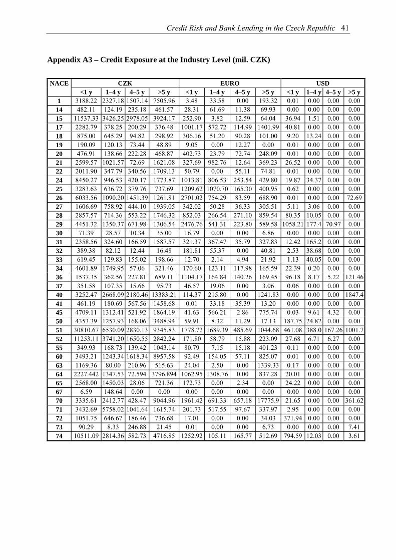
Credit Risk and Bank Lending in the Czech Republic 41
Appendix A3 – Credit Exposure at the Industry Level (mil. CZK)
CZK EURO USDNACE<1 y 1–4 y 4–5 y >5 y <1 y 1–4 y 4–5 y >5 y <1 y 1–4 y 4–5 y >5 y
1 3188.22 2327.18 1507.14 7505.96 3.48 33.58 0.00 193.32 0.01 0.00 0.00 0.0014 482.11 124.19 235.18 461.57 28.31 61.69 11.38 69.93 0.00 0.00 0.00 0.0015 11537.33 3426.25 2978.05 3924.17 252.90 3.82 12.59 64.04 36.94 1.51 0.00 0.0017 2282.79 378.25 200.29 376.48 1001.17 572.72 114.99 1401.99 40.81 0.00 0.00 0.0018 875.00 645.29 94.82 298.92 306.16 51.20 90.28 101.00 9.20 13.24 0.00 0.0019 190.09 120.13 73.44 48.89 9.05 0.00 12.27 0.00 0.01 0.00 0.00 0.0020 476.91 138.66 222.28 468.87 402.73 23.79 72.74 248.09 0.01 0.00 0.00 0.0021 2599.57 1021.57 72.69 1621.08 327.69 982.76 12.64 369.23 26.52 0.00 0.00 0.0022 2011.90 347.79 340.56 1709.13 50.79 0.00 55.11 74.81 0.01 0.00 0.00 0.0024 8450.27 946.53 420.17 1773.87 1013.81 806.53 253.54 429.80 19.87 34.37 0.00 0.0025 3283.63 636.72 379.76 737.69 1209.62 1070.70 165.30 400.95 0.62 0.00 0.00 0.0026 6033.56 1090.20 1451.39 1261.81 2701.02 754.29 83.59 688.90 0.01 0.00 0.00 72.6927 1606.69 758.92 444.10 1939.05 342.02 50.28 36.33 305.51 5.11 3.06 0.00 0.0028 2857.57 714.36 553.22 1746.32 852.03 266.54 271.10 859.54 80.35 10.05 0.00 0.0029 4451.32 1350.37 671.98 1306.54 2476.76 541.31 223.80 589.58 1058.21 177.4 70.97 0.0030 71.39 28.57 10.34 35.00 16.79 0.00 0.00 6.86 0.00 0.00 0.00 0.0031 2358.56 324.60 166.59 1587.57 321.37 367.47 35.79 327.83 12.42 165.2 0.00 0.0032 389.38 82.12 12.44 16.48 181.81 55.37 0.00 40.81 2.53 38.68 0.00 0.0033 619.45 129.83 155.02 198.66 12.70 2.14 4.94 21.92 1.13 40.05 0.00 0.0034 4601.89 1749.95 57.06 321.46 170.60 123.11 117.98 165.59 22.39 0.20 0.00 0.0036 1537.35 362.56 227.81 689.11 1104.17 164.84 140.26 169.45 96.18 8.17 5.22 121.4637 351.58 107.35 15.66 95.73 46.57 19.06 0.00 3.06 0.06 0.00 0.00 0.0040 3252.47 2668.09 2180.46 13383.21 114.37 215.80 0.00 1241.83 0.00 0.00 0.00 1847.441 461.19 180.69 567.56 1458.68 0.01 33.18 35.39 13.20 0.00 0.00 0.00 0.0045 4709.11 1312.41 521.92 1864.19 41.63 566.21 2.86 775.74 0.03 9.61 4.32 0.0050 4353.39 1257.93 168.06 3488.94 59.91 8.32 11.29 17.13 187.75 24.82 0.00 0.0051 30810.67 6530.09 2830.13 9345.83 1778.72 1689.39 485.69 1044.68 461.08 388.0 167.26 1001.752 11253.11 3741.20 1650.55 2842.24 171.80 58.79 15.88 223.09 27.68 6.71 6.27 0.0055 349.93 168.73 139.42 1043.14 80.79 7.15 15.18 401.23 0.11 0.00 0.00 0.0060 3493.21 1243.34 1618.34 8957.58 92.49 154.05 57.11 825.07 0.01 0.00 0.00 0.0063 1169.36 80.00 210.96 515.63 24.04 2.50 0.00 1339.33 0.17 0.00 0.00 0.0064 2227.442 1347.53 72.594 3796.894 1062.95 1308.76 0.00 837.28 20.01 0.00 0.00 0.0065 2568.00 1450.03 28.06 721.36 172.73 0.00 2.34 0.00 24.22 0.00 0.00 0.0067 6.59 148.64 0.00 0.00 0.00 0.00 0.00 0.00 0.00 0.00 0.00 0.0070 3335.61 2412.77 428.47 9044.96 1961.42 691.33 657.18 17775.9 21.65 0.00 0.00 361.6271 3432.69 5758.02 1041.64 1615.74 201.73 517.55 97.67 337.97 2.95 0.00 0.00 0.0072 1051.75 646.67 186.46 736.68 17.01 0.00 0.00 34.03 371.94 0.00 0.00 0.0073 90.29 8.33 246.88 21.45 0.01 0.00 0.00 6.73 0.00 0.00 0.00 7.4174 10511.09 2814.36 582.73 4716.85 1252.92 105.11 165.77 512.69 794.59 12.03 0.00 3.61

42 Narcisa Kadlčáková, Joerg Keplinger
Appendix A4 – Loan Interest Rates at the Industry Level
NACE Implicit Loan Interest rate1 16.30%
14 6.23%15 8.65%17 9.27%18 11.88%19 11.72%20 7.76%21 6.79%22 7.81%24 9.18%25 9.90%26 11.49%27 10.29%28 12.63%29 11.14%30 1.66%31 15.56%32 19.12%33 8.80%34 28.29%36 7.87%37 14.73%40 13.96%41 3.06%45 9.83%50 9.63%51 9.63%52 9.63%55 7.03%60 16.30%63 16.30%64 16.30%65 16.30%67 16.30%70 11.05%71 11.05%72 11.05%73 11.05%74 11.05%

Credit Risk and Bank Lending in the Czech Republic 43
Appendix A5 – Asset Return Correlations
NACE 1 14 15 17 18 20 21 22 24 25 26
1 1.0014 -0.77 1.0015 0.49 0.01 1.0017 0.56 -0.60 0.15 1.0018 0.06 -0.31 -0.10 0.53 1.0020 0.20 -0.10 0.28 0.68 0.55 1.0021 0.26 -0.66 -0.59 0.25 0.23 -0.13 1.0022 0.61 -0.88 -0.02 0.60 0.62 0.27 0.53 1.0024 0.23 -0.57 -0.51 0.05 -0.17 -0.30 0.73 0.35 1.0025 0.55 -0.52 0.25 0.88 0.30 0.68 0.14 0.47 0.05 1.0026 -0.77 0.90 -0.06 -0.76 -0.25 -0.37 -0.52 -0.76 -0.51 -0.69 1.0027 0.70 -0.68 0.17 0.89 0.36 0.61 0.38 0.62 0.20 0.77 -0.8528 -0.21 0.51 0.49 0.17 0.27 0.55 -0.71 -0.26 -0.86 0.26 0.3829 -0.15 0.28 0.38 0.27 0.41 0.64 -0.66 0.03 -0.64 0.32 0.1330 0.39 -0.56 -0.05 0.88 0.51 0.64 0.21 0.61 0.17 0.77 -0.7231 0.43 -0.73 -0.24 0.76 0.47 0.39 0.51 0.73 0.44 0.62 -0.7732 0.42 -0.38 0.34 0.77 0.47 0.75 -0.21 0.52 -0.14 0.71 -0.5933 -0.56 0.65 -0.17 -0.01 -0.10 0.15 -0.37 -0.64 -0.43 0.02 0.4834 0.62 -0.79 0.11 0.82 0.72 0.55 0.36 0.91 0.17 0.66 -0.7936 0.12 -0.36 0.07 0.42 0.72 0.42 -0.05 0.66 -0.06 0.30 -0.3137 -0.07 -0.37 -0.45 0.01 0.54 -0.08 0.46 0.57 0.42 -0.24 -0.1940 -0.56 0.36 -0.36 -0.56 0.05 -0.47 -0.04 -0.27 -0.24 -0.70 0.5441 -0.77 0.86 -0.13 -0.89 -0.38 -0.48 -0.44 -0.77 -0.35 -0.81 0.9645 -0.15 0.35 0.32 0.34 0.47 0.73 -0.56 -0.09 -0.59 0.27 0.0950 -0.65 0.75 -0.18 -0.91 -0.60 -0.66 -0.29 -0.80 -0.13 -0.78 0.8651 -0.67 0.94 0.10 -0.73 -0.38 -0.28 -0.60 -0.86 -0.55 -0.62 0.9455 -0.73 0.92 -0.04 -0.76 -0.39 -0.32 -0.50 -0.85 -0.44 -0.61 0.9360 -0.74 0.91 -0.02 -0.77 -0.35 -0.38 -0.53 -0.82 -0.50 -0.71 0.9764 -0.73 0.90 -0.14 -0.61 -0.46 -0.21 -0.44 -0.90 -0.34 -0.45 0.8270 0.24 -0.15 0.31 0.50 0.24 0.53 -0.18 0.21 -0.15 0.54 -0.3071 0.20 -0.25 0.07 0.34 0.17 0.19 0.11 0.25 0.10 0.31 -0.2672 -0.57 0.77 0.07 -0.67 -0.40 -0.36 -0.48 -0.72 -0.38 -0.56 0.8274 -0.30 0.45 0.17 -0.41 -0.25 -0.19 -0.35 -0.39 -0.24 -0.31 0.50

44 Narcisa Kadlčáková, Joerg Keplinger
Asset Return Correlations – continue
NACE 27 28 29 30 31 32 33 34 36 37 40
11415171820212224252627 1.0028 -0.06 1.0029 0.05 0.81 1.0030 0.76 0.07 0.37 1.0031 0.71 -0.25 0.04 0.91 1.0032 0.64 0.38 0.67 0.84 0.60 1.0033 -0.20 0.48 0.32 0.00 -0.24 -0.09 1.0034 0.77 -0.01 0.24 0.81 0.81 0.74 -0.43 1.0036 0.23 0.21 0.60 0.59 0.52 0.68 -0.26 0.71 1.0037 0.03 -0.43 -0.07 0.20 0.39 0.05 -0.41 0.42 0.60 1.0040 -0.60 -0.10 -0.18 -0.51 -0.40 -0.52 0.06 -0.39 -0.12 0.25 1.0041 -0.91 0.19 -0.02 -0.82 -0.82 -0.69 0.37 -0.86 -0.38 -0.12 0.5845 0.17 0.75 0.81 0.35 0.02 0.60 0.42 0.22 0.41 -0.11 -0.1950 -0.87 -0.03 -0.28 -0.87 -0.80 -0.82 0.31 -0.93 -0.59 -0.23 0.4651 -0.77 0.43 0.12 -0.77 -0.87 -0.57 0.51 -0.84 -0.46 -0.39 0.4255 -0.82 0.35 0.06 -0.77 -0.84 -0.63 0.52 -0.88 -0.47 -0.35 0.4260 -0.80 0.33 0.07 -0.76 -0.83 -0.61 0.49 -0.84 -0.42 -0.26 0.5364 -0.68 0.32 0.03 -0.60 -0.70 -0.53 0.64 -0.87 -0.53 -0.45 0.3170 0.43 0.34 0.43 0.47 0.28 0.58 0.06 0.38 0.32 -0.15 -0.4771 0.32 0.01 0.08 0.29 0.26 0.26 -0.05 0.30 0.20 0.04 -0.2972 -0.69 0.27 0.02 -0.71 -0.76 -0.55 0.37 -0.76 -0.40 -0.31 0.3374 -0.40 0.21 0.06 -0.45 -0.50 -0.28 0.13 -0.42 -0.18 -0.20 0.10

Credit Risk and Bank Lending in the Czech Republic 45
0%
5%
10%
15%
20%
25%
30%
Y1 Y2 Y3 Y4 Y5 Y6
Class1Class2Class3Class4Class5Class6Class7
Asset Return Correlations – continue
NACE 41 45 50 51 55 60 64 70 71 72 74
114151718202122242526272829303132333436374041 1.0045 -0.03 1.0050 0.93 -0.28 1.0051 0.93 0.18 0.86 1.0055 0.93 0.09 0.89 0.96 1.0060 0.96 0.07 0.88 0.96 0.92 1.0064 0.81 0.12 0.79 0.86 0.91 0.81 1.0070 -0.40 0.40 -0.47 -0.28 -0.30 -0.32 -0.21 1.0071 -0.31 0.06 -0.31 -0.29 -0.29 -0.27 -0.24 0.88 1.0072 0.81 0.02 0.78 0.82 0.81 0.82 0.74 0.12 0.24 1.0074 0.48 0.02 0.46 0.49 0.48 0.49 0.42 0.49 0.62 0.88 1
Appendix A6 – Rating Class-Specific Credit Spreads

CNB Working Papers Series
6/2004 Narcisa Kadlčáková:Joerg Keplinger
Credit risk and bank lending in the Czech Republic
5/2004 Petr Král: Identification and measurement of relationships concerninginflow of FDI: The case of the Czech Republic
4/2004 Jiří Podpiera: Consumers, consumer prices and the Czech business cycleidentification
3/2004 Anca Pruteanu: The role of banks in the Czech monetary policy transmissionmechanism
2/2004 Ian Babetskii: EU enlargement and endogeneity of some OCA criteria:Evidence from the CEECs
1/2004 Alexis Derviz:Jiří Podpiera
Predicting bank CAMELS and S&P ratings: The case of theCzech Republic
12/2003 Tibor Hlédik: Modelling the second-round effects of supply-side shocks oninflation
11/2003 Luboš Komárek:Zdeněk ČechRoman Horváth
ERM II membership – the view of the accession countries
10/2003 Luboš Komárek:Zdeněk ČechRoman Horváth
Optimum currency area indices – how close is the CzechRepublic to the eurozone?
9/2003 Alexis Derviz:Narcisa KadlčákováLucie Kobzová
Credit risk, systemic uncertainties and economic capitalrequirements for an artificial bank loan portfolio
8/2003 Tomáš Holub:Martin Čihák
Price convergence: What can the Balassa–Samuelson modeltell us?
7/2003 Vladimír Bezděk:Kamil DybczakAleš Krejdl
Czech fiscal policy: Introductory analysis
6/2003 Alexis Derviz: FOREX microstructure, invisible price determinants, and thecentral bank’s understanding of exchange rate formation
5/2003 Aleš Bulíř: Some exchange rates are more stable than others: short-runevidence from transition countries
4/2003 Alexis Derviz: Components of the Czech koruna risk premium in a multiple-dealer FX market
3/2003 Vladimír Benáček:Ladislav ProkopJan Á. Víšek
Determining factors of the Czech foreign trade balance:Structural Issues in Trade Creation
2/2003 Martin Čihák:Tomáš Holub
Price convergence to the EU: What do the 1999 ICP datatell us?
1/2003 Kamil Galuščák:Daniel Münich
Microfoundations of the wage inflation in the Czech Republic

4/2002 Vladislav Flek:Lenka MarkováJiří Podpiera
Sectoral productivity and real exchange rate appreciation:Much ado about nothing?
3/2002 Kateřina Šmídková:Ray Barrell DawnHolland
Estimates of fundamental real exchange rates for the five EUpre-accession countries
2/2002 Martin Hlušek: Estimating market probabilities of future interest rate changes
1/2002 Viktor Kotlán: Monetary policy and the term spread in a macro model of asmall open economy

Czech National BankEconomic Research DepartmentNa Příkopě 28, 115 03 Praha 1
Czech Republicphone: +420 2 244 12 321
fax: +420 2 244 14 278e-mail: [email protected]


