Working hours mismatch and well-being: comparative ... · Working hours mismatch and well-being:...

Working hours mismatch and well-being: comparative evidence fromAustralian and German panel data

Franziska KuglerIfo Institute Munich

Andrea WiencierzUniversity of York

Christoph WunderUniversity of Erlangen-Nuremberg

(October 2014)

LASER Discussion Papers - Paper No. 82

(edited by A. Abele-Brehm, R.T. Riphahn, K. Moser and C. Schnabel)

Correspondence to:

Christoph Wunder, Lange Gasse 20, 90403 Nuremberg, Germany, Email:[email protected].

Abstract

This study uses subjective measures of well-being to analyze how workers perceive working hoursmismatch. Our particular interest is in the question of whether workers perceive hours ofunderemployment differently from hours of overemployment. Previous evidence on this issue isambiguous. We call attention to the level of well-being in the absence of hours mismatch that serves asa reference state for comparison purposes and to the consequences of restrictive functional formassumptions. Using panel data from Australia and Germany, this study estimates the relationshipbetween working hours mismatch and well-being as a bivariate smooth function of desired hours andmismatch hours by tensor product p-splines. The results indicate that well-being is highest in theabsence of hours mismatch. In general, the perception of overemployment is statistically significantlydifferent from the perception of underemployment in both countries. In Australia, workers toleratesome underemployment, as their well-being tends to be unaltered in the presence of short hours ofunderemployment. However, the marginal loss from underemployment appears to be larger than thatfrom overemployment once the mismatch exceeds approximately ten hours. In Germany, on thecontrary, underemployment is clearly more detrimental for well-being than overemployment. Germanmales with preferences for full-time hours hardly respond to overemployment.

Copyright statement

This document has been posted for the purpose of discussion and rapid dissemination of preliminaryresearch results.

Working hours mismatch and well-being: comparative evidence from

Australian and German panel data

Franziska Kugler

Ifo Institute Munich

Andrea Wiencierz

University of York

Christoph Wunder

University of Erlangen-Nuremberg

October 13, 2014

Abstract

This study uses subjective measures of well-being to analyze how workers perceive working

hours mismatch. Our particular interest is in the question of whether workers perceive hours of

underemployment differently from hours of overemployment. Previous evidence on this issue

is ambiguous. We call attention to the level of well-being in the absence of hours mismatch that

serves as a reference state for comparison purposes and to the consequences of restrictive func-

tional form assumptions. Using panel data from Australia and Germany, this study estimates

the relationship between working hours mismatch and well-being as a bivariate smooth func-

tion of desired hours and mismatch hours by tensor product p-splines. The results indicate that

well-being is highest in the absence of hours mismatch. In general, the perception of overem-

ployment is statistically significantly different from the perception of underemployment in both

countries. In Australia, workers tolerate some underemployment, as their well-being tends to be

unaltered in the presence of short hours of underemployment. However, the marginal loss from

underemployment appears to be larger than that from overemployment once the mismatch ex-

ceeds approximately ten hours. In Germany, on the contrary, underemployment is clearly more

detrimental for well-being than overemployment. German males with preferences for full-time

hours hardly respond to overemployment.

Keywords: life satisfaction, job satisfaction, working hours mismatch, semi-parametric regres-

sion, bivariate smoothing

JEL Classification: I31, J21, J22

Corresponding author: Christoph Wunder, University of Erlangen-Nuremberg, Department of

Economics, Lange Gasse 20, 90403 Nuremberg, Germany. Tel.: +49 911 5302 260; Fax: +49

911 5302 178. Email: [email protected]

Acknowledgements: We thank participants of the ESPE Conference 2014, of the SOEP Confer-

ence 2014, of the EALE Conference 2014, of seminars at the IOS Regensburg and the IAAEU

Trier as well as Fabian Scheipl for helpful comments and stimulating discussions.

1 Introduction

Many workers all over the world want to adjust their hours of work but are not able to do so.

They experience a working hours mismatch between actual and desired hours of work.1 Only

recently, researchers focused increased attention to the question of how workers subjectively

perceive a situation in which they are not able to realize their desired hours of work. However,

the findings of previous studies for different countries are inconclusive, as there is evidence

for negative, insignificant, or positive relationships between well-being and hours mismatch

(Friedland and Price 2003, Wooden et al. 2009, Baslevent and Kirmanoglu 2013, Wunder and

Heineck 2013). Even studies that agree on the sign of the correlation are still ambiguous as to

whether overemployment or underemployment is more strongly related to well-being. On the

one hand, different results for different countries may reflect true differences, for example, in

institutional settings or attitudes. Such knowledge may help to shed light on the mechanisms

through which hours mismatch impinges on well-being. On the other hand, however, different

results may be an artifact of different modeling approaches. Furthermore, applying particular

functional form assumptions, studies may be overly restrictive to depict the underlying relation.

This study examines the subjective perception of working hours mismatch using informa-

tion about workers’ subjective well-being (SWB). Our particular interest is in the question of

whether workers perceive hours of underemployment differently from hours of overemploy-

ment. We argue that measurement of the perception of hours mismatch should be based on a

precise definition of the level of well-being in the absence of hours mismatch that serves as

1 A large body of empirical research reports working hours mismatch for many countries (e.g., Altonji and

Paxson 1988, Dickens and Lundberg 1993, Stewart and Swaffield 1997, Euwals and Van Soest 1999, Bell and

Freeman 2001). Otterbach (2010) provides evidence on mismatches between actual and desired hours of work

in 21 countries, including France, Germany, the UK, Russia, and the US.

1

a reference state for comparison purposes. Previous studies use (implicitly defined) different

reference states, which may be a further source of ambiguity in empirical findings.

This paper contributes to the literature by providing first comparative evidence from lon-

gitudinal data on the perception of mismatches for two countries within a unified analysis

framework. We explicitly discuss the reference state for comparison, which determines the

measurement of the well-being penalty of hours mismatch, and employ a semiparamteric es-

timation approach that does not rely on functional form assumption about the relationship be-

tween well-being and hours mismatch. This approach avoids overly-restrictive functional form

assumptions by modeling this relationship as a bivariate smooth function of desired hours and

mismatch hours. Furthermore, using smooth functions allows us to measure the well-being

penalty in greater detail than previous studies while the graphical representation of results is

easy to interpret.

In this paper, we focus on a comparison between Australia and Germany—two countries

for which rich longitudinal panel data sets, the Household, Income and Labour Dynamics in

Australia (HILDA) Survey and the German Socio-Economic Panel (SOEP), gather information

about actual and desired hours of work.2 In general, the results indicate that well-being is high-

est in the absence of hours mismatch. We find some evidence for an asymmetrical perception of

underemployment and overemplyoment among Australians. Their well-being is stable between

the onset of underemployment and approximately five hours of underemployment. However,

the well-being function tends to be steeper for underemployment than overemployment once

the ten-mismatch hours threshold is exceeded, pointing to a larger marginal loss in well-being

from underemployment than from overemployment in the region of many mismatch hours. In

contrast, underemployment is clearly more detrimental for well-being than overemployment in

2 Such detailed information is not available, for instance, in the British Household Panel Survey (BHPS), which

only asks whether individuals want to work longer (or shorter) hours.

2

Germany over the entire distribution of mismatch hours. In particular, well-being declines im-

mediately with the onset of underemployment. The finding that German males hardly respond

to overemployment may explain the large share of approximately 60% of overemployed male

workers in Germany. Since their expected utility gains from adjusting their working hours are

rather small, they do not have strong incentives to leave overemployment.

2 Literature review

Labor market-related factors are among the most extensively investigated characteristics in the

literature on SWB. Previous research has provided ample evidence on the role played by indi-

vidual unemployment (e.g., Clark and Oswald 1994, Gerlach and Stephan 1996, Winkelmann

and Winkelmann 1998), unemployment duration (Clark 2006), unemployment rates (Di Tella

et al. 2003, Luechinger et al. 2010), and earnings (Clark et al. 2009, Wunder and Schwarze

2009, Card et al. 2012). Further evidence indicates that long working hours are correlated with

a decline in SWB (Clark et al. 1996, Sousa-Poza and Sousa-Poza 2003, Fahr 2011) and health

(e.g., Sparks et al. 1997, Amagasa and Nakayama 2012, Virtanen et al. 2012).

Recent research has started to focus attention on working hours mismatch. Table 1 provides

an overview of the studies reviewed. In general, studies find worse health among mismatched

workers than among those with working hours match. For instance, Friedland and Price (2003)

report an increased number of chronic conditions among mismatched workers in the US. Us-

ing German and British panel data, Bell et al. (2011) find negative effects of working hours

mismatch, in particular of overemployment, on health satisfaction and self-assessed health. For

Great Britain, Constant and Otterbach (2011) detect negative consequences of working hours

mismatch for mental health measures, with overemployment appearing to be a more severe

problem than underemployment.

3

There is also a growing body of international literature on the relationship between work-

ing hours mismatch and job or life satisfaction. For the US, Friedland and Price (2003) reveal

lower job satisfaction among overemployed workers whereas underemployed workers are, sur-

prisingly, more satisfied than matched ones. Life satisfaction appears to be unaffected by mis-

matches. For the UK, results based on data from the British Household Panel Survey (BHPS)

suggest that overemployment lowers job and life satisfaction by more than underemployment

(Green and Tsitsianis 2005). In Japan, overemployment is associated with lower job satisfac-

tion whereas underemployment is not significantly correlated with job satisfaction among fe-

males (Boyles and Shibata 2009). Using data from the European Social Survey, Baslevent and

Kirmanoglu (2013) show that the reduction in life satisfaction associated with working hours

mismatch is smaller in countries with higher unemployment rates.

Using data from the first wave of the HILDA Survey in 2001, Wilkins (2007) finds a negative

correlation of underemployment and life (job) satisfaction for part-time employees. In contrast,

underemployment does generally not matter for SWB of full-time employees. However, un-

deremployed male full-time employees are an exception, as they report lower life satisfaction

than matched male full-time employees. Wooden et al. (2009) estimate individual fixed effects

models of life and job satisfaction with HILDA data from 2001 to 2005.3 The study reveals that

well-being in general varies only little with the actual hours of work per week, once working

time mismatches are taken into account. Overemployed males suffer a well-being penalty of up

to 0.4 points on the 11-point scale, on average. The penalty is even larger for overemployed fe-

males and overemployed workers who already work long hours (more than 41 hours per week).

Underemployed part-time employees experience a considerable decline in job and life satis-

3 Their econometric model includes a set of indicator variables that represent categories of actual hours of work

by working hours mismatch (i.e. for persons who want to work more than, less than or in accordance with their

desired hours of work).

4

faction while underemployed males with standard or above standard hours do not report lower

well-being than matched workers (with standard hours). Interestingly, underemployed women

working 41 to 49 hours per week report even higher job satisfaction than those with working

hours match in the category between 35 and 40 hours per week. This suggests that under-

employment is especially detrimental for those with short working hours. In a refined model

specification that includes variables measuring the extent of the mismatch in hours (instead of

indicator variables), the study reports that the (negative) coefficients of underemployment and

overemployment are not statistically different, at least for job satisfaction. Nevertheless, the

authors conclude that overemployment is a more serious problem than underemployment for

Australian workers.

For Germany, the empirical evidence indicates lower job satisfaction among mismatched

workers than among matched workers. Using data from the SOEP for 1985 to 2002, Green and

Tsitsianis (2005) find that overemployment is more detrimental for job satisfaction than under-

employment in West Germany while underemployment has a stronger negative effect in East

Germany. A cross-section analysis for 2004 reveals significant negative correlations between

mismatch hours and life, job and health satisfaction (Grözinger et al. 2008). Likewise, using

SOEP data for 1984 to 2003, Cornelißen (2009) shows that an increase of mismatch hours

results in a decline of job satisfaction. Hanglberger (2010) estimates the effects of hours of

underemployment and overemployment separately with SOEP data from 2005 and 2007. Job

satisfaction is lower among underemployed part-time employees than among overemployed

part-time employees, though the difference may not be significantly different. The coefficients

of the mismatch variables are insignificant among full-time employees. Using SOEP data cov-

ering the period 1985 to 2011, Wunder and Heineck (2013) show that the decline in life sat-

5

isfaction is clearly larger for underemployment than for overemployment. Also, they provide

evidence on spillovers from the partner’s mismatch onto the other partner’s well-being.

The studies reviewed for Germany and Australia could be improved in several aspects. In

particular, the following drawbacks call into question the validity of results and limit compara-

bility. First, applying a rather restricted specification with indicator variables for underemploy-

ment and overemployment, studies only capture the average difference between mismatched

workers and matched workers. The average loss in well-being is, however, determined by the

(average) extent of underemployment or overemployment. The observation that the coefficient

of the overemployment indicator variable is larger (in absolute terms) than that of the underem-

ployment indicator is not informative about the marginal loss (i.e. the loss per mismatch hour).

Hence, a larger coefficient may just reflect that the average number of hours of overemploy-

ment is higher than the average number of hours of underemployment. Second, using only one

variable measuring the difference between actual and desired hours as an explanatory variable,

studies ignore potentially differential roles played by underemployment and overemployment,

respectively. Third, the comparability of evidence is considerably limited because studies look

at different population subgroups and results are based on different model specifications. Fi-

nally, studies might be too inflexible by assuming that a linear estimation equation is sufficient

to describe the relationship between working hours mismatch and well-being.

3 Conceptual framework and estimation model

3.1 Measuring well-being change: what is the reference state?

This section introduces a framework for measuring how SWB changes when mismatch hours

change. The key idea is that measurement requires a comparison between SWB in the presence

of mismatch and SWB in the absence of mismatch. The latter represents the reference state for

6

comparison purposes. We discuss two possible reference states that lead to different measures

for the SWB change: the first reference state defines the absence of mismatch as a state in

which a counterfactual choice set of work hours includes the worker’s observed desired hours

of work. Thus, one compares SWB between states that have the same desired hours but different

actual hours. The second reference state defines the absence of mismatch as a state in which

counterfactual desired hours are consistent with the observed hours choice. Thus, one compares

SWB between states that have the same actual hours but different desired hours.

Figure 1 illustrates our considerations using a conventional neoclassical labor supply frame-

work. The worker’s preferences are represented by a utility function U(G,H,e), where G is a

composite good and H denotes actual hours of market work. The parameter e represents inter-

personal differences in preferences for consumption and work. Hence, two workers may reach

different utility levels from the same consumption-hours bundle.

The worker chooses hours of work subject to the budget constraint to maximize well-being

(or utility). If working time is continuous over the interval [0,T ], the worker achieves the

optimal level of well-being at desired hours of work H1, where the indifference curve I1 is just

tangent to the budget constraint. However, firms may offer only jobs with fixed hours because of

legal regulations, firm-specific requirements, or collective bargaining agreements, for instance.

Therefore, the choice set is restricted to a discrete set of hours.4 For parsimony of explanation,

we assume that firms offer only jobs with actual hours H0. The difference between desired

hours and actual hours indicates the hours mismatch M = H1 −H0. If M > 0, the worker is

4 Among others, Altonji and Paxson (1988) and Dickens and Lundberg (1993) develop frameworks where work-

ers receive job offers consisting of fixed wage-hours combinations. In this case, workers adjust their working

time by selecting wage-hours combinations across employers offering different job packages. Working time

mismatches may be persistent over time when the worker has, for example, imperfect information about job

opportunities and changing jobs is costly. In such a situation, the worker will only change the job if the utility

gain exceeds search and mobility costs. As a consequence, we may observe persistent mismatches in the labor

market unless utility gains are sufficiently large (Altonji and Paxson 1992).

7

underemployed, as he or she accepts a job offer with shorter working time than the desired

hours of work. If M < 0, the worker is overemployed, as he or she accepts a job offer with

longer working time than the desired hours of work.

A first candidate measure of the change in SWB associated with the hours mismatch com-

pares the utility level of the mismatched worker, as indicated by I0 in Figure 1, with the utility

level the mismatched worker would have reached, had he or she been able to choose the working

time according to desired hours, as indicated by I1. The reference state is defined by the SWB

level when M = 0 while holding desired hours fixed in the comparison. Since M = H1 −H0,

changes in actual hours, H0, are the only source of variation in mismatch hours, M. Thus, the

change in SWB is indicative for the effect of hours constraints that determine actual hours but

not desired hours.

Empirical studies, however, almost exclusively use a second candidate measure for the

change in SWB, as they hold fixed actual hours of work. That is, the second measure com-

pares the utility of the mismatched worker, as indicated by I0, and the utility level the worker

would have reached, had his or her desired hours of work been equal to actual hours offered,

as indicated by I2. The reference state is defined by the SWB level when M = 0 while holding

fixed actual hours or work. Here, changes in desired hours are the source of variation in mis-

match hours. In consequence, the change in SWB is indicative about the association between

SWB and working time preferences.

Which references state is appropriate to measure the loss in well-being associated with hours

mismatch? We propose that it is more interesting to use the first measure that holds desired

hours (or preferences) fixed. In this case, the mismatch results from restrictions in hours of

work choices because these are the only source of variation in mismatch hours when desired

hours are controlled for. Thus, we may obtain an idea for a re-design of working time arrange-

8

ments: should we re-design working time arrangements to primarily avoid underemployment

or overemployment or both?

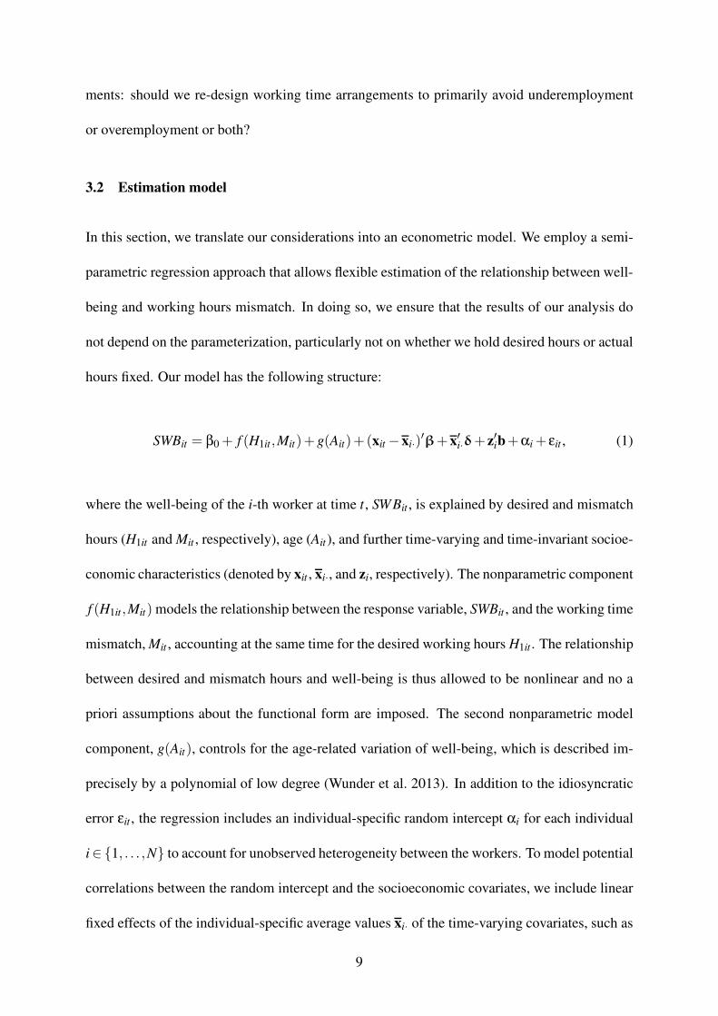
3.2 Estimation model

In this section, we translate our considerations into an econometric model. We employ a semi-

parametric regression approach that allows flexible estimation of the relationship between well-

being and working hours mismatch. In doing so, we ensure that the results of our analysis do

not depend on the parameterization, particularly not on whether we hold desired hours or actual

hours fixed. Our model has the following structure:

SWBit = β0 + f (H1it,Mit)+g(Ait)+(xit −xi·)′β+x′i·δ+ z′ib+αi + εit , (1)

where the well-being of the i-th worker at time t, SWBit , is explained by desired and mismatch

hours (H1it and Mit , respectively), age (Ait), and further time-varying and time-invariant socioe-

conomic characteristics (denoted by xit , xi·, and zi, respectively). The nonparametric component

f (H1it,Mit) models the relationship between the response variable, SWBit , and the working time

mismatch, Mit , accounting at the same time for the desired working hours H1it . The relationship

between desired and mismatch hours and well-being is thus allowed to be nonlinear and no a

priori assumptions about the functional form are imposed. The second nonparametric model

component, g(Ait), controls for the age-related variation of well-being, which is described im-

precisely by a polynomial of low degree (Wunder et al. 2013). In addition to the idiosyncratic

error εit , the regression includes an individual-specific random intercept αi for each individual

i∈ {1, . . . ,N} to account for unobserved heterogeneity between the workers. To model potential

correlations between the random intercept and the socioeconomic covariates, we include linear

fixed effects of the individual-specific average values xi· of the time-varying covariates, such as

9

household income, marital status of the worker, or type of occupation, as was suggested, e.g.,

by Mundlak (1978). For each worker i, the vector xi· is given by 1Ti

∑t(i,Ti)

t=t(i,1)xit , where Ti is the

number of observations of worker i and t(i,1), . . . , t(i,Ti) denote the ordered observation times of

this worker. To obtain a better interpretability, we simultaneously include the demeaned co-

variate vector (xit − xi·). Finally, there are some linear effects of time-invariant covariates zi,

including period effects.

The model is a linear additive mixed model with a normally distributed random intercept,

i.e., we assume that α= (α1, . . . ,αN)′ with α∼N (0,σ2

α IN), where IN is the N×N identity ma-

trix and 0 is a vector of zeros of the corresponding length. The errors εit are also assumed to be

independent and identically distributed random quantities, each following a normal distribution

with mean 0 and variance σ2ε . Hence, the error vector ε follows the multivariate normal distri-

bution ε∼ N (0,σ2ε In), where n = ∑N

i=1 Ti. Moreover, we assume that α and ε are independent

from each other and are not correlated with the covariates.

The smooth function g is modeled as a cubic regression spline with 9 basis functions defined

according to Wood (2006, section 4.1.2), while the bivariate function f is represented by a 200

dimensional tensor product spline based on marginal cubic regression splines. We estimate both

smooth functions as penalized splines, which can be represented in the mixed model framework.

Therefore, we estimate all model components simultaneously as empirical best linear predictors

of the corresponding linear mixed model with restricted maximum likelihood (REML) estima-

tion for the variance components, which yields consistent estimates of all model components.

For further details about the underlying statistical methodology, see, e.g., Fahrmeir et al. (2013,

Chapter 8) or Wood (2006, Chapter 6).

As we are particular interested in the question whether over- and underemployment are

associated with subjective well-being in the same way, we furthermore reformulate the model

10

in Equation 1 as follows

SWBit = β0 + f1(H1it, |Mit|)+ f2(H1it ,M+it )+g(Ait)+(xit −xi·)

′β+x′i·δ+ z′ib+αi + εit , (2)

where |Mit| denotes the absolute value of Mit , while M+it equals Mit when Mit > 0 and is zero

otherwise. This reformulation allows us to test whether underemployment (corresponding to

Mit > 0) is associated with well-being in a different way than overemployment. If the smooth

term f2 contributes to the model in a significant way, we conclude that workers perceive hours

of underemployment differently from hours of overemployment. All models are fit within the

statistical software environment R (R Core Team 2013) by the function gamm() of the mgcv-

Package (Wood 2013) with option REML.

4 Data

We use longitudinal data from the Household, Income and Labour Dynamics in Australia

(HILDA) Survey and the German Socio-Economic Panel (SOEP). For detailed information

about the surveys, see Wooden and Watson (2007) and Wagner et al. (2007), respectively. Since

working time issues are at the core of this analysis, we restrict the estimation samples to indi-

viduals of main working age (20 to 60 years) who are employed at the time of the survey. To

ensure comparability of the Australian and the German data, we further restrict the samples to

the period 2001 to 2012 that is covered in both surveys. After deleting cases with incomplete

data on the variables of interest, the Australian samples consist of 8,750 females and 9,046

males, and the German samples consist of 11,597 females and 12,047 males. Both surveys

provide detailed information on the socio-economic characteristics of respondents, including

age, disability status, relationship status, citizenship, education, job characteristics (branch of

11

industry, occupation), income, and household size. Tables 2 and 3 provide descriptive statistics

for subsamples by gender.

We use questions about life satisfaction to measure well-being of workers. The respective

questions are formulated similarly in the HILDA Survey and the SOEP. Life satisfaction is

ascertained by asking: “All things considered, how satisfied are you with your life?” Answers

are collected on 11-point scales ranging from 0 (completely dissatisfied) to 10 (completely

satisfied). Figure 2 shows the gender-specific distribution of life satisfaction for both Germany

and Australia. In the SOEP, female (male) respondents report an average level of 7.1 (7.1) for

life satisfaction. The corresponding values in the HILDA Survey are 7.9 (7.8). In both surveys,

the median is 7, and the most frequent score (mode) in the sample is 8.5

Next, we describe the distribution of actual hours of work. Table 4 reports the percentage

of the employed workforce in five working hours categories. In general, female labor supply is

concentrated in lower categories of actual hours of work while male labor supply is clustered

in upper categories (>36). Interestingly, short (< 20) and very long (> 52) hours of work are

reported more frequently by Australians than by Germans. The dispersion in hours is higher in

Australia than in Germany while hours of work tend to be more concentrated around 40 hours

per week in Germany.

Desired hours of work are also recorded in a comparable fashion in both surveys: “If you

could choose your own number of working hours, taking into account that your income would

change according to the number of hours: How many hours would you want to work?” Using the

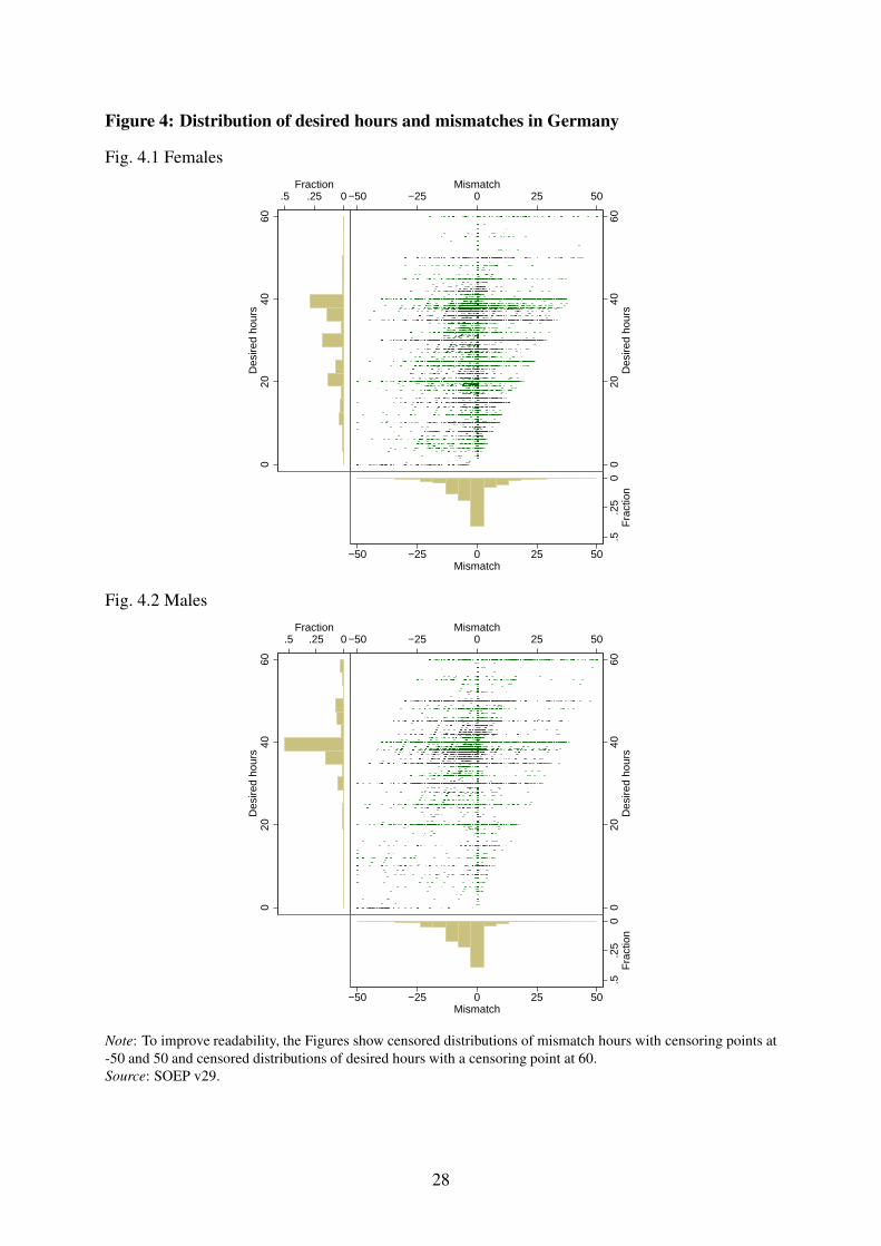
information about the actual and desired hours, we calculate the hours mismatch. Figures 3 and

4 graphically summarize the bivariate distribution of desired hours of work and hours mismatch.

5 We provide additional results for job satisfaction in the Appendix. The job satisfaction question is: “How

satisfied are you with your job?” In the SOEP, female (male) respondents report an average level of 7.0 (7.0)

for job satisfaction. The corresponding values in the HILDA Survey are 7.7 (7.5).

12

Australian females want to work around full-time and part-time hours. Roughly 40% of

the female workforce reports mismatch: 27% are overemployed, 15% are underemployed. For

Australian males, desired hours are concentrated around full-time hours, though long and short

hours are also desired. Also about 40% of the male workforce reports mismatch: 30% are

overemployed, 12% are underemployed. German females, similar to Australian females, want

to work full-time or part-time hours, but longer hours are hardly desired. With 72% of the

female workforce reporting hours mismatch, German females are clearly more often unable

to realize their working hours preferences than Australian females. 51% are overemployed,

21% are underemployed. German males predominantly want to work full-time hours while

they desire neither long nor short hours. More than 70% of the male workforce reports hours

mismatch, with 61% being overemployed and 12% being underemployed.

5 Results

5.1 Interpretation of contour plots and general pattern

This section discusses the results from the bivariate smoothing. Figures 5 to 8 show the results

for the model in Equation 1 in the form of contour plots of the bivariate smooth functions by

country and gender. In addition, the Figures show a univariate plot of the level of life satisfaction

as a function of mismatch hours holding fixed desired hours at values of 30 and 40 hours for

females and males, respectively.6 The bivariate smooths estimate the well-being for different

combinations of desired hours of work and hours mismatch. The SWB levels are represented by

a color gradient from yellow to red, with yellow indicating higher well-being und red indicating

lower well-being.

6 Tables A1 to A4 in the Appendix show the full estimation results for the parametric components.

13

The plots offer three interpretations. (1) A horizontal movement from left to right first

shows well-being of overemployed workers (M < 0), then well-being of underemployed work-

ers (M > 0). Since desired hours of work are constant along the horizontal direction, the hor-

izontal movement compares states with identical working time preferences but different actual

hours. Thus, the results are indicative about changes in SWB associated with constraints in

hours of work choices. (2) A diagonal movement along a 45 degree line shows the change in

SWB associated with mismatches holding actual hours fixed. In this way, the plots allow to

compare SWB in states with equal actual hours of works and different working time prefer-

ences. However, as we argue in section 3, it is more interesting to learn about the changes in

SWB from restricted choices because choice sets may be changed by policy intervention and

firms’ working time regulations. (3) A vertical movement indicates the well-being for simul-

taneous changes in actual hours of work and desired hours of work, holding hours mismatch

constant.

In general, well-being is highest across all subsamples in the absence of mismatch. The

vertical movement at zero mismatch hours provides some evidence for negative relationship

between SWB and working hours for Australian workers (Figures 5.1 and 6.1). Their life

satisfaction declines until approximately 30 hours but does not change for working hours of

more than 30 hours. Among German females, SWB does virtually not change over the entire

range of working hours (Figure 7.1). For German males, the empirical evidence shows even a

positive trend in SWB for long working hours (Figure 8.1).7 Overall, the small variation in SWB

in the absence of hours mismatch suggests that working hours appear to be rather unimportant

for SWB, as long as workers are able to realize their desired hours of work. Previous studies

provide similar evidence of either no or a positive relationship between actual hours and SWB

7 For clarification, Figures A2.1 to A2.4 in the Appendix show univariate functions of the level of life satisfaction

and working hours, setting hours mismatch to zero.

14

once the hours mismatch is controlled for (e.g., Friedland and Price 2003, Green and Tsitsianis

2005). In contrast, studies that do not control for hours mismatch usually report a negative

relationship between working hours and SWB (e.g., Clark et al. 1996).

Regarding the relationship between SWB and hours mismatch, a test of differences in the

perception of hours of underemployment and hours of overemployment provides convincing

evidence that that workers generally perceive hours of underemployment differently from hours

of overemployment. The test assesses the statistical significance of the smooth term f2 in Equa-

tion 2 (see section 3.2), which is significant in all subsamples with p-values<0.000. Generally,

SWB tends to decline as one moves from the area of matched hours (center) to the area of

overemployment (left) or the the area of underemployment (right). The decline in well-being

is more pronounced in the regions where preferences are concentrated (i.e. for average desired

hours) while the decline is less pronounced for short and long working hours preferences.

5.2 Australian females

The analysis shows two noteworthy results for the well-being of mismatched Australian fe-

males. First, in the area of part-time working hours between 20 and 30 hours, short hours

of overemployment appear to be more detrimental for well-being than short hours of under-

emplyoment among Australian females (see, Figure 5.1). While the level of life satisfaction

associated with overemployment of five hours (given a working time preference of 30 hours) is

significantly lower than that of a matched worker (i.e. 7.75 vs. 7.84, with non-overlapping 90%

confidence intervals (CIs) of [7.699,7.801] and [7.802,7.886], respectively), the level associated

with five hours of underemployment is 7.82 (90% CI: [7.781,789]), which is not significantly

different from the SWB of matched workers.

[Insert Figure 5 about here]

15

Second, this pattern is reversed for longer mismatch hours, as the decline in life satisfaction

is stronger for underemployment than for overemployment once a threshold of approximately

ten mismatch hours is crossed. Assuming average desired hours of about 30, we cross seven

contour lines in the area of underemployment and only four in the area of overemplyoment

when we move beyond ten hours of mismatch. In correspondence, the spacing of the contour

lines is closer in the area of underemployment than in the area of overemployment. Therefore,

the decline in life satisfaction associated with an increase in underemployment is higher than

that associated with an increase in overemployment once the ten-hours threshold is exceeded.

Figure 5.2 depicts the mismatch-SWB relationship given a working time preference of 30

hours. For ten or less mismatch hours, the decline in life satisfaction is stronger in the area

of overemployment than in the area of underemployment. Once the ten-hours threshold is

exceeded, we observe the reverse pattern, as the curve is steeper for underemployment than

overemployment.

Since the SWB penalty of overemployment occurs already at a low number of hours mis-

match, overemployed females experience lower well-being than underemployed females over a

wide range of hours mismatches. Females with overemployment of, e.g., 10 hours are less sat-

isfied with their lives than females with equal-sized underemployement. For average working

hours preferences of 30 hours, overemployed females who actually work 40 hours are at the 7.7

contour line while underemployed females who actually work 20 hours are at the 7.8 contour

line.8

8 In general, the analysis of job satisfaction provides qualitatively equivalent results (see, Figure A1 in the Ap-

pendix).

16

5.3 Australian males

Australian males reach the highest level of life satisfaction when they are able to work their

desired number of hours. A vertical movement in Figure 6.1 shows that a simultaneous increase

in actual hours and desired hours of work correlates with a decline in life satisfaction in the

region of preferences for short working hours (below 20). Then, well-being is unchanged when

hours further increase, suggesting that the hours of work hardly affect well-being as long as

working hours preferences are met.


As with Australian females, the decline in well-being occurs earlier in the case of overem-

ployment than with underemployment among Australian males. Thus, we observe a stronger

decline in life satisfaction among overemployed workers than among underemployed workers.

For example, with a preference for full time employment of 40 hours per week and a mismatch

of five hours, life satisfaction of overemployed workers is statistically significantly lower than

that of matched workers (7.68 vs. 7.77, with non-overlapping 90% CIs of [7.636,7.718] and

[7.731,7.801], respectively). In contrast, we do not find significant differences between un-

deremployed workers, who want to increase their working time by five hours, and matched

workers.

This result is also evident from the univariate plot in Figure 6.2, which reveals the mismatch-

SWB relationship holding fixed working time preferences at 40 hours. The curve has a steeper

slope for short hours of overemployment than for short hours of underemployment, suggesting

that Australian males are more sensitive towards overemployment than underemployment for

hours mismatch of up to approximately ten hours.

17

5.4 German females

The evidence for German females clearly shows that underemployment is more detrimental

for well-being than overemployment. This result is in contrast to the evidence provided for

Australia. For working hours preferences of 30 hours and ten mismatch hours, for exam-

ple, underemployed females reach a level of life satisfaction of 7.02 (90% CI: [6.966,7.063])

whereas overemployed females with an equal-sized hours mismatch reach a level of 7.11 (90%

CI: [7.069,7.150]).


Well-being of mismatched female workers is characterized by two findings. First, the de-

cline in well-being starts already at a small number of hours of underemployment. Second, the

decline in well-being is stronger for underemployment than overemployment, as we move over

more contour lines in the right part than in the left part of Figures 7.1. The mismatch interval

between zero and ten hours covers four contour lines in the right part (underemployment) and

only two in the left part (overemployment), given average desired hours. The alternative graph-

ical representation in Figure 7.2 also depicts the asymmetrical perception of underemployment

and overemplyoment for fixed working time preferences of 30 hours. Thus, the partial effect

of constraints in work hours choice appears to be larger for underemployment than for overem-

ployment.9

9 For job satisfaction, the evidence very clearly confirms that underemployment is more detrimental than overem-

ployment. However, in contrast to life satisfaction, the decline associated with underemployment start at a

higher number of the hours of underemployment. Thus, tolerance against underemployment appears to be

higher in terms of job satisfaction than in terms of life satisfaction. Interestingly, we do not find any response

in job satisfaction to overemployment for females with preferences for long working hours. The contour lines

are almost horizontally for 40 or more desired hours (see, Figure A1.3 in the Appendix).

18

5.5 German males

The most striking result emerges from the data for German males. Here, evidence for lower

well-being among overemployed workers is scarce or nonexistent. In particular, workers with

preferences for long working hours hardly respond to overemployment. In Figures 8.1, the con-

tour lines in the upper left (representing overemployed workers with preferences for long hours)

tend to be horizontal, suggesting almost unchanged life satisfaction with varying overemploy-

ment hours.


This pattern clearly changes in the area of underemployment where contour lines tend to be

vertical, indicating declining well-being with further increases in underemployment (see right

part of Figure 8.1). Thus, the decline in SWB is clearly stronger for underemployed workers

than for overemployed workers. In consequence, a worker who wants to work 40 hours but

actually works 50 hours reaches a level of life satisfaction of 7.09 (90% CI: [7.056,7.132])

while a worker with the same preference (i.e. who also wants to work 40 hours) but whose

actual working hours are 30 hours has life satisfaction of 6.85 (90% CI: [6.783,6.925]). Among

male workers, overemployment seems to be important only when the worker has preferences

for short hours.

Figure 8.2 shows the response to mismatch hours holding fixed working time preferences at

40 hours. The curve is almost flat in the area of overemployment (M < 0) while it has a steep

slope in the area of overemployment (M > 0).

6 Conclusion

This study leads to several conclusions. First, we conclude that previous research has drawn too

little attention to the nonlinear nature of the relationship between SWB and hours mismatch.

19

This study used highly flexible semiparametric regressions to measure the SWB penalty of hours

mismatch in new detail. The findings demonstrate that the relative effects of underemployment

and overemployement cannot be reliably measured in a model framework that uses overly-

restrictive functional form assumptions. Model specifications that use only indicator variables

for overemployment and underemployment obviously do not reveal with precision how workers

perceive working hours mismatch.

Second, we conclude that the measurement of the SWB penalty of hours mismatch depends

on the assumption about the reference state in the absence of mismatch used for comparison

purposes. Our conceptual framework provides arguments for comparing SWB between states

that have the same desired hours but different actual hours. Hence, we argued to assess the SWB

penalty of hours mismatch holding fixed desired hours. Because the choice of the reference state

has consequences for measuring the SWB penalty from hours mismatch, this paper hopefully

starts a discussion on the choice of the reference state, which previous research did not make

clear.

Third, our findings provide an explanation for the large share of about 60% of overemployed

males in Germany. Overemployed German males do not experience substantially lower life

satisfaction than matched ones. We conclude that only small gains in utility will arise from

eliminating or reducing overemployment. In consequence, overemployed workers do not have

incentives to leave the mismatch due to the small (expected) increase in SWB.

Fourth, the finding that overemployment is less important than underemployment in Ger-

many while the opposite applies to Australia leads us to the conclusion that internal labor mar-

kets are a more important vehicle for career advancement in Germany than in Australia (Lazear

and Oyer 2004). If high level jobs are allocated through internal labor markets, then overem-

20

ployed workers will accept long hours of work although job offers do not match their working

time preferences.

Overall, our analysis shows that hours mismatch resulting from hours of work restrictions

is related to substantial losses in SWB. Therefore, an assessment of the labor market condi-

tions should take account of the extent to which workers are able to adjust their hours of work

according to their preferences. We propose to improve matches between actual and desired

hours of work, as there are potential increases in workers’ well-being. From a worker’s point

of view, reducing hours mismatch could contribute to enhancing the work-life-balance and the

reconciliation of work and family life. From an employer’s view, reducing hours mismatch

could comprise the advantage that more satisfied employees are healthier, more productive, and

more committed to the firm. To achieve this, employers could, for example, offer more flexible

working time schemes to meet workers’ desired hours.

21

References

Altonji, J. G. and Paxson, C. H. (1988). Labor supply preferences, hours constraints, and hours-

wage trade-offs. Journal of Labor Economics, 6(2):254–276.

Altonji, J. G. and Paxson, C. H. (1992). Labor supply, hours constraints, and job mobility. The

Journal of Human Resources, 27(2):256–278.

Amagasa, T. and Nakayama, T. (2012). Relationship between long working hours and de-

pression in two working populations: A structural equation model approach. Journal of

Occupational and Environmental Medicine, 54(7):868–874.

Baslevent, C. and Kirmanoglu, H. (2013). The impact of deviations from desired hours of work

on the life satisfaction of employees. Social Indicators Research, Online:1–11.

Bell, D. N., Otterbach, S., and Sousa-Poza, A. (2011). Work hours constraints and health. IZA

Discussion Papers 6126, Institute for the Study of Labor (IZA).

Bell, L. A. and Freeman, R. B. (2001). The incentive for working hard: explaining hours worked

differences in the US and Germany. Labour Economics, 8(2):181–202.

Boyles, C. and Shibata, A. (2009). Job satisfaction, work time, and well-being among married

women in japan. Feminist Economics, 15(1):57–84.

Card, D., Mas, A., Moretti, E., and Saez, E. (2012). Inequality at work: The effect of peer

salaries on job satisfaction. American Economic Review, 102(6):2981–3003.

Clark, A. E. (2006). A note on unhappiness and unemployment duration. Applied Economics

Quarterly (formerly: Konjunkturpolitik), 52(4):291–308.

Clark, A. E., Kristensen, N., and Westergård-Nielsen, N. (2009). Job satisfaction and co-worker

wages: Status or signal? Economic Journal, 119(536):430–447.

Clark, A. E., Oswald, A., and Warr, P. (1996). Is job satisfaction U-shaped in age? Journal of

Occupational & Organizational Psychology, 96(1):57–81.

Clark, A. E. and Oswald, A. J. (1994). Unhappiness and unemployment. Economic Journal,

104(424):648–59.

Constant, A. F. and Otterbach, S. (2011). Work hours constraints: Impacts and policy implica-

tions. IZA Policy Papers 35, Institute for the Study of Labor (IZA).

Cornelißen, T. (2009). The interaction of job satisfaction, job search, and job changes - an

empirical investigation with German panel data. Journal of Happiness Studies, 10(3):367–

384.

Di Tella, R., MacCulloch, R. J., and Oswald, A. J. (2003). The macroeconomics of happiness.

The Review of Economics and Statistics, 85(4):809–827.

Dickens, W. T. and Lundberg, S. J. (1993). Hours restrictions and labor supply. International

Economic Review, 34(1):pp. 169–192.

Euwals, R. and Van Soest, A. (1999). Desired and actual labour supply of unmarried men and

women in the Netherlands. Labour Economics, 6(1):95–118.

22

Fahr, R. (2011). Job design and job satisfaction – empirical evidence for Germany? manage-

ment revue. Socio-economic Studies, 22(1):28–46.

Fahrmeir, L., Kneib, T., Lang, S., and Marx, B. (2013). Regression: Models, Methods and

Applications. Springer, Berlin.

Friedland, D. and Price, R. (2003). Underemployment: Consequences for the health and well-

being of workers. American Journal of Community Psychology, 32:33–45.

Gerlach, K. and Stephan, G. (1996). A paper on unhappiness and unemployment in Germany.

Economics Letters, 52:325–330.

Green, F. and Tsitsianis, N. (2005). An investigation of national trends in job satisfaction in

Britain and Germany. British Journal of Industrial Relations, 43(3):401–429.

Grözinger, G., Matiaske, W., and Tobsch, V. (2008). Arbeitszeitwünsche, Arbeitslosigkeit

und Arbeitszeitpolitik. SOEPpapers 103, DIW Berlin, The German Socio-Economic Panel

(SOEP).

Hanglberger, D. (2010). Arbeitszufriedenheit und flexible arbeitszeiten: empirische analyse

mit daten des sozio-oekonomischen panels. SOEPpapers on Multidisciplinary Panel Data

Research 304, DIW Berlin, The German Socio-Economic Panel (SOEP).

Lazear, E. P. and Oyer, P. (2004). Internal and external labor markets: a personnel economics

approach. Labour Economics, 11(5):527–554.

Luechinger, S., Meier, S., and Stutzer, A. (2010). Why does unemployment hurt the employed?:

Evidence from the life satisfaction gap between the public and the private sector. Journal of

Human Resources, 45(4):998–1045.

Mundlak, Y. (1978). On the pooling of time series and cross section data. Econometrica,

46(1):69–85.

Otterbach, S. (2010). Mismatches between actual and preferred work time: Empirical evidence

of hours constraints in 21 countries. Journal of Consumer Policy, 33(2):143–161.

R Core Team (2013). R: A Language and Environment for Statistical Computing. R Foundation

for Statistical Computing. Used R version 2.15.2.

Sousa-Poza, A. and Sousa-Poza, A. A. (2003). Gender differences in job satisfaction in Great

Britain, 1991-2000: permanent or transitory? Applied Economics Letters, 10(11):691–694.

Sparks, K., Cooper, C., Fried, Y., and Shirom, A. (1997). The effects of hours of work on

health: A meta-analytic review. Journal of Occupational and Organizational Psychology,

70(4):391–408.

Stewart, M. B. and Swaffield, J. K. (1997). Constraints on the desired hours of work of British

men. Economic Journal, 107(441):520–535.

Virtanen, M., Heikkilä, K., Jokela, M., Ferrie, J. E., Batty, G. D., Vahtera, J., and Kivimäki,

M. (2012). Long working hours and coronary heart disease: A systematic review and meta-

analysis. American Journal of Epidemiology, 176(7):586–596.

23

Wagner, G. G., Frick, J. R., and Schupp, J. (2007). The German Socio-Economic Panel Study

(SOEP) – scope, evolution and enhancemants. Schmollers Jahrbuch (Journal of Applied

Social Science Studies), 127(1):139–169.

Wilkins, R. (2007). The consequences of underemployment for the underemployed. Journal of

Industrial Relations, 49(2):247–275.

Winkelmann, L. and Winkelmann, R. (1998). Why are the unemployed so unhappy? Evidence

from panel data. Economica, 65(257):1–15.

Wood, S. N. (2006). Generalized Additive Models: An Introduction with R. Chapman &

Hall/CRC.

Wood, S. N. (2013). mgcv: Mixed GAM Computation Vehicle with GCV/AIC/REML smoothness

estimation. R package version 1.7-27.

Wooden, M., Warren, D., and Drago, R. (2009). Working time mismatch and subjective well-

being. British Journal of Industrial Relations, 47(1):147–179.

Wooden, M. and Watson, N. (2007). The HILDA Survey and its contribution to economic and

social research (so far). The Economic Record, 83(261):208–231.

Wunder, C. and Heineck, G. (2013). Working time preferences, hours mismatch and well-being

of couples: Are there spillovers? Labour Economics, 24:244–252.

Wunder, C. and Schwarze, J. (2009). Income inequality and job satisfaction of full-time em-

ployees in Germany. Journal of Income Distribution, 18(2):70–91.

Wunder, C., Wiencierz, A., Schwarze, J., and Küchenhoff, H. (2013). Well-being over the life

span: Semiparametric evidence from British and German longitudinal data. The Review of

Economics and Statistics, 95(1):154–167.

24

Appendix: Figures and Tables

Figure 1: Labor supply and hours mismatches

H

G

0 TH1 H0

I0I1 I2

b

b

25

Figure 2: Distribution of life satisfaction in Australia and Germany

0.1

.2.3

.4

0 1 2 3 4 5 6 7 8 9 10

AU: life satisfaction

Males Females

0.1

.2.3

.4

0 1 2 3 4 5 6 7 8 9 10

DE: life satisfaction

Males Females

Source: HILDA v12, SOEP v29.

26

Figure 3: Distribution of desired hours and mismatches in Australia

Fig. 3.1 Females

020

4060

Des

ired

hour

s

0.25.5Fraction

020

4060

Des

ired

hour

s

−50 −25 0 25 50Mismatch

0.2

5.5 F

ract

ion

−50 −25 0 25 50Mismatch

Fig. 3.2 Males

020

4060

Des

ired

hour

s

0.25.5Fraction

020

4060

Des

ired

hour

s−50 −25 0 25 50

Mismatch0

.25

.5 Fra

ctio

n

−50 −25 0 25 50Mismatch

Note: To improve readability, the Figures show censored distributions of mismatch hours with censoring points at

-50 and 50 and censored distributions of desired hours with a censoring point at 60.

Source: HILDA v12.

27

Figure 4: Distribution of desired hours and mismatches in Germany

Fig. 4.1 Females

020

4060

Des

ired

hour

s

0.25.5Fraction

020

4060

Des

ired

hour

s

−50 −25 0 25 50Mismatch

0.2

5.5

Fra

ctio

n

−50 −25 0 25 50Mismatch

Fig. 4.2 Males

020

4060

Des

ired

hour

s

0.25.5Fraction

020

4060

Des

ired

hour

s−50 −25 0 25 50

Mismatch0

.25

.5F

ract

ion

−50 −25 0 25 50Mismatch

Note: To improve readability, the Figures show censored distributions of mismatch hours with censoring points at

-50 and 50 and censored distributions of desired hours with a censoring point at 60.

Source: SOEP v29.

28

Figure 5: Results for Australian females

Fig. 5.1: Bivariate smooth of desired hours and mismatch hours

−30 −20 −10 0 10 20 30

010

2030

4050

60

Mismatch hours

Des

ired

hour

s 7.5

7.55

7.6

7.6

5

7.65

7.7

7.7

7.75

7.75

7.8

7.8

7.85

7.85

7.9 7.95

Fig. 5.2: Life satisfaction and mismatch hours holding fixed desired hours at 30

−30 −20 −10 0 10 20 30

7.5

7.6

7.7

7.8

7.9

8.0

Mismatch hours

Pre

dict

ed li

fe s

atis

fact

ion

Note: Contour plots of bivariate smooth functions based on Equation 1. The SWB levels are represented by

a color gradient from yellow to red, with yellow indicating higher well-being und red indicating lower well-

being. Negative mismatch hours (M < 0) indicate overemployment while positive mismatch hours (M > 0) indicate

underemployment. The dotted lines indicate 90% approximate point-wise confidence intervals.

Source: HILDA v12, SOEP v29, 2001-2012.

29

Figure 6: Results for Australian males


−30 −20 −10 0 10 20 30

010

2030

4050

60

Mismatch hours

Des

ired

hour

s

7.5

7.55

7.6

7.65

7.65

7.7

7.75

7.75 7

.8

7.8 7

.85

7.9


−30 −20 −10 0 10 20 30

7.3

7.4

7.5

7.6

7.7

7.8

Mismatch hours

Pre

dict

ed li

fe s

atis

fact

ion






30

Figure 7: Results for German females


−30 −20 −10 0 10 20 30

010

2030

4050

60

Mismatch hours

Des

ired

hour

s

6.7

6.7

6.7

5

6.75

6.8 6.8

6.8

5

6.85

6.9

6.9

6.9

5

6.9

5

6.95

7

7

7.0

5

7.05

7.1

7.1 7.15

7.15

7.15

7.2

7.2


−30 −20 −10 0 10 20 30

6.8

6.9

7.0

7.1

7.2

7.3

Mismatch hours

Pre

dict

ed li

fe s

atis

fact

ion






31

Figure 8: Results for German males


−30 −20 −10 0 10 20 30

010

2030

4050

60

Mismatch hours

Des

ired

hour

s 6.4

6.45

6.5

6.55

6.6

6.6

5

6.65

6.8

5 6

.9

6.95

6.9

5

7 7

7.05

7.1

7.15

7.2

7.25


−30 −20 −10 0 10 20 30

6.8

6.9

7.0

7.1

7.2

7.3

Mismatch hours

Pre

dict

ed li

fe s

atis

fact

ion






32

Table 1: Overview of studies on working hours mismatch

Study Data Outcome(s) Model and estimation Results

Baslevent and

Kirmanoglu (2013)

Europe, European

Social Survey 2010,

employees only

life satisfaction

(11-point scale)

hours of underemployment and hours of

overemployment, ordered logistic model

• underemployment: -0.02

• overemployment: -0.01

• smaller effects if high unemployment rate

Bell et al. (2011) Germany, SOEP 1992 -

2008

health satisfaction

(11-point scale),

self-assessed health

(5-point scale)

indicator variables that represent categories of

actual hours of work by working hours

mismatch type (underemployment,

overemployment or match), linear fixed

effects regression, fixed effects ordered logit

• underemployment: -0.0 to -0.3

(self-assessed health)

• overemployment: -0.0 to -0.5 (health

satisfaction and self-assessed health)

Boyles and Shibata

(2009)

Japan, data collected

by Japan Institute of

Life Insurance in 1991,

married women (20 -

44 years)

job satisfaction

(4-point scale)

dummy for underemployment, dummy for

overemployment, logistic regressions

• underemployment: insignificant


Constant and Otterbach

(2011)

UK, BHPS 1991 - 2007 mental health

(depression, stress)





effects regressions

• underemployment: -0.05 to -0.12

(depressions), -0.03 to -0.05 (stress)

• overemployment: -0.06 to -0.13

(depressions), -0.07 to -0.21 (stress)

Cornelißen (2009) Germany, SOEP, 1985,

1987, 1989, 1995,

2001, employees, West

German workers

(16-60 years)

job satisfaction

(11-point scale)

number of mismatch hours, pooled ordered

probit, linear fixed effects regression

• mismatch hours: job satisfaction (-0.01)

Friedland and Price

(2003)

US, Americans’

Changing Lives (ACL)

study 1986, 1989, 25

years and older,

persons in the labor

force

health measures,

psychological

well-being, job and life

satisfaction


overemployment, hierarchical regressions

• underemployment: -0.043 (positive

self-concept), 0.075 (job satisfaction),

insignificant (life satisfaction)

• overemployment: +0.049 (chronic

disease), -0.063 (job satisfaction),

insignificant (life satisfaction)

Green and Tsitsianis

(2005)

Germany, SOEP

1985-2002, partly

1991-2002

job satisfaction

(11-point scale)


overemployment, linear fixed effects

regression

• underemployment: West -0.16 / East -0.10

• overemployment: West -0.20 / East -0.00

33

Study Data Outcome(s) Model and estimation Results

Green and Tsitsianis

(2005)

UK, BHPS 1992-2002 job satisfaction

(7-point scale)



regression

• underemployment: -0.15,


Grözinger et al. (2008) Germany, SOEP 2004 job, life, and health

satisfaction (11-point

scale)

number of mismatch hours, cross section

analysis, ordered probit

• mismatch hours: -0.01 to -0.18 (job, life

and health satisfaction)

Hanglberger (2010) Germany, SOEP 2005

– 2007, separated for

part-time and full-time

employees

job satisfaction

(11-point scale)



regression, control for working time variables

regarding overtime, night work, etc.

• part-time and underemployment: -0.04

• part-time and overemployment: -0.03

• full-time: insignificant coefficients

Wilkins (2007) Australia, HILDA 2001 job and life satisfaction

(11-point scale)

dummy for underemployment, cross section

analysis

• part-time and underemployment: life and

job satisfaction (-0.4)

• full-time and underemployment: life and

job satisfaction (insign., exc. men’s life

satisfaction)

Wooden et al. (2009) Australia, HILDA 2001

– 2005, 15 years and

older, partly only

employed persons

job and life satisfaction

(11-point scale)





effects regression

• number of working hours unimportant for

SWB

• males and underemployment: -0.4 (job

satisfaction, esp. part-time)

• males and overemployment: -0.1 to -0.4

(job and life satisfaction)

• females and underemployment: -0.3 (job

satisfaction, part-time), +1.0 (job

satisfaction, part-time)

• females and overemployment: -0.1 to -0.6

(job and life satisfaction)

Wunder and Heineck

(2013)

Germany, SOEP 1985

– 2011, couples (both

employed, 30 – 60

years)

life satisfaction

(11-point scale)



regression, IV regression

• underemployment: -0.01 to -0.02 (females

and males)

• females and overemployment: -0.01,

• males and overemployment: insign.,

• partner’s underemployment: -0.01,

• partner’s overemployment: insign.

34

Table 2: Descriptive statistics: HILDA

Females Males

Variable Mean Std. Dev. Mean Std. Dev.

Life satisfaction 7.88 1.29 7.82 1.31

Job satisfaction 7.70 1.70 7.54 1.68

Actual hours 32.80 13.50 43.56 12.27

Desired hours 31.00 11.33 40.97 10.91

Overemployed 0.27 0.45 0.30 0.46

Underemployed 0.15 0.36 0.12 0.33

Overemployment (in hours) 3.44 6.87 4.01 7.66

Underemployment (in hours) 1.64 4.76 1.41 4.64

Log of wage 3.04 0.51 3.16 0.55

Log of household size 0.98 0.50 0.98 0.53

Log of yearly non-labor hh income 10.12 2.64 9.49 2.99

Born outside Australia 0.20 0.40 0.21 0.41

Age 39.01 11.14 38.67 11.12

Disabled 0.15 0.36 0.15 0.35

Educ: Postgraduate degree 0.05 0.21 0.05 0.22

Educ: Graduate diploma 0.08 0.28 0.05 0.23

Educ: Bachelor degree 0.21 0.40 0.16 0.37

Educ: Diploma 0.11 0.31 0.09 0.29

Educ: Certificate level III and IV 0.16 0.37 0.29 0.46

Educ: Finished year 12 0.17 0.38 0.16 0.37

Educ: Finished year 11 or less 0.22 0.42 0.19 0.39

Married 0.50 0.50 0.53 0.50

Defacto 0.18 0.38 0.18 0.38

Separated 0.03 0.18 0.02 0.16

Divorced 0.08 0.26 0.04 0.19

Widowed 0.01 0.10 0.002 0.04

Single 0.20 0.40 0.22 0.42

Number of dependent children 0.63 0.96 0.69 1.03

Occ.: Missing or other 0.00 0.00 0.00 0.00

Occ.: Managers 0.08 0.28 0.15 0.35

Occ.: Professionals 0.27 0.44 0.18 0.39

Occ.: Technicians 0.19 0.39 0.14 0.34

Occ.: Clerical support workers 0.21 0.41 0.08 0.27

Occ.: Service and sales workers 0.17 0.37 0.08 0.27

Occ.: Skilled agricultural workers 0.00 0.07 0.02 0.15

Occ.: Craft workers 0.01 0.08 0.16 0.37

Occ.: Operators and assemblers 0.01 0.12 0.11 0.31

Occ.: Elementary 0.06 0.24 0.08 0.27

NACE: Missing or other 0.01 0.12 0.01 0.12

NACE: Agriculture and mining 0.03 0.18 0.09 0.28

NACE: Manufacturing 0.03 0.16 0.09 0.29

NACE: Electricity and gas supply 0.01 0.09 0.04 0.18

NACE: Water supply/construction 0.02 0.14 0.12 0.33

NACE: Trade, Retail 0.19 0.40 0.18 0.38

NACE: Information/finance 0.08 0.27 0.12 0.33

NACE: Administration activities 0.18 0.39 0.20 0.40

NACE: Education 0.39 0.49 0.11 0.31

NACE: Arts, entertainment 0.05 0.22 0.04 0.20

Number of persons 7,768 8,047

Number of person-year observations 34,424 37,099

Source: HILDA v12, 2001-2012.

35

Table 3: Descriptive statistics: SOEP

Females Males

Variable Mean Std. Dev. Mean Std. Dev.

Life satisfaction 7.13 1.62 7.13 1.57

Job satisfaction 7.05 1.98 7.03 1.96

Actual hours 32.85 12.91 44.28 9.74

Desired hours 30.48 10.10 39.5 7.66

Underemployed 0.21 0.41 0.12 0.32

Overemployed 0.51 0.50 0.61 0.49

Underemployment (in hours) 1.85 4.79 0.91 3.72

Overemployment (in hours) 4.21 6.33 5.69 7.41

Log of wage 2.39 0.59 2.64 0.61

Log of household size 0.95 0.45 0.99 0.49

Log of monthly non-labor income 6.41 2.63 5.46 2.89

Foreign citizenship 0.06 0.23 0.07 0.25

Age 41.75 10.39 41.88 10.30

Disabled 0.05 0.22 0.06 0.24

Education in years 12.68 2.64 12.69 2.77

Married 0.61 0.49 0.64 0.48

Divorced 0.12 0.33 0.09 0.28

Widowed 0.02 0.14 0.004 0.06

Single 0.24 0.43 0.27 0.44

Number of children LE16 0.56 0.84 0.68 0.96

east 0.24 0.43 0.22 0.42

NACE: Missing 0.04 0.21 0.04 0.19

NACE: Other 0.01 0.09 0.02 0.13

NACE: Agriculture and mining 0.02 0.15 0.03 0.17

NACE: Manufacturing 0.06 0.25 0.17 0.38

NACE: Electricity and gas supply 0.04 0.20 0.11 0.31

NACE: Water supply/construction 0.02 0.14 0.11 0.31

NACE: Trade, Retail 0.18 0.38 0.11 0.31

NACE: Information/finance 0.08 0.27 0.11 0.31

NACE: Administration activities 0.17 0.38 0.17 0.38

NACE: Education 0.31 0.46 0.09 0.29

NACE: Arts, entertainment 0.07 0.26 0.05 0.22

Occ.: Missing 0.03 0.17 0.03 0.17

Occ.: Managers 0.04 0.19 0.08 0.28

Occ.: Professionals 0.17 0.37 0.20 0.40

Occ.: Technicians 0.30 0.46 0.17 0.38

Occ.: Clerical support workers 0.17 0.37 0.07 0.25

Occ.: Service and sales workers 0.17 0.37 0.04 0.20

Occ.: Skilled agricultural workers 0.01 0.09 0.01 0.11

Occ.: Craft workers 0.03 0.17 0.23 0.42

Occ.: Operators and assemblers 0.02 0.15 0.10 0.31

Occ.: Elementary 0.07 0.26 0.05 0.23

Number of persons 11,597 12,047

Number of person-year observations 52,390 56,973

Source: SOEP v29, 2001-2012.

36

Table 4: Distribution of actual hours per week (% of employed workforce)

Actual hours of work

<20 20-35 36-43 44-51 >52

Australia

Female 17.5 31.6 33.5 12.3 5.1

Male 3.9 9.5 41.0 27.9 17.8

Germany

Female 16.5 32.0 34.6 13.3 3.6

Male 1.9 5.9 46.1 30.8 15.2Source: HILDA v12, SOEP v29.

37

Appendix

Supplementary material for

Working hours mismatch and well-being:

comparative evidence from Australian and German panel data

Contents

Job satisfaction as bivariate smooth function of desired hours and mismatch hours by

subsample 39

Life satisfaction and working hours in the absence of mismatch 40

Estimation results: HILDA, females 41

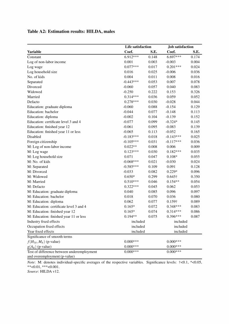
Estimation results: HILDA, males 42

Estimation results: SOEP, females 43

Estimation results: SOEP, males 44

Figure A1: Job satisfaction as bivariate smooth function of desired hours and mismatch hours by subsample

Fig. A1.1: Australian females Fig. A1.2: Australian males

−30 −20 −10 0 10 20 30

010

2030

4050

60

mismatch

desi

red

hour

s

6.8

6.9

7

7

7.1

7.2

7.2

7.3

7.3

7.4 7.4

7.5

7.5

7.6

7.6 7.7

7.7

7.8

7.8

7.9

7.9

8

8.1

−30 −20 −10 0 10 20 30

010

2030

4050

60

mismatch

desi

red

hour

s

6.7 6.8

6.9 7

7.1

7.1

7.2

7.2

7.3

7.3

7.4

7.4

7.5

7.5

7.6

7.7

Fig. A1.3: German females Fig. A1.4: German males

−30 −20 −10 0 10 20 30

010

2030

4050

60

mismatch

desi

red

hour

s

6.7

6.8

6.9

6.9

7

7

7.1

7.1

7.1

7.2

7.2

7.4

7.4

7.5 7.6

7.7

7.8

7.9

−30 −20 −10 0 10 20 300

1020

3040

5060

mismatch

desi

red

hour

s

6.1

6

.3

6.4 6.

5

6.6

6.7

6.8

6.9

6.9

7

7

7

7.1

7.1

7.2

7.2

7.2

7.3

7.6

7.7

7.8

7.9

8

Note: Contour plots of bivariate smooth functions based on Equation 1. The SWB levels are represented by a color gradient from yellow to red, with yellow indicating higher

well-being und red indicating lower well-being. Negative mismatch hours (M < 0) indicate overemployment while positive mismatch hours (M > 0) indicate underemployment.

Calculation for median values of covariates.


Figure A2: Life satisfaction and working hours in the absence of mismatch

Fig. A2.1: Australian females Fig. A2.2: Australian males

0 10 20 30 40 50 60

7.6

7.8

8.0

8.2

8.4

Working hours

Pre

dict

ed li

fe s

atis

fact

ion

0 10 20 30 40 50 60

7.6

7.8

8.0

8.2

8.4

Working hours

Pre

dict

ed li

fe s

atis

fact

ion

Fig. A2.3: German females Fig. A2.4: German males

0 10 20 30 40 50 60

6.6

6.8

7.0

7.2

7.4

Working hours

Pre

dict

ed li

fe s

atis

fact

ion

0 10 20 30 40 50 60

6.6

6.8

7.0

7.2

7.4

Working hours

Pre

dict

ed li

fe s

atis

fact

ion

Note: The smooths show the level of life satisfaction as a function of working hours setting mismatch hours to zero (i.e. in the absence of mismatch).


Table A1: Estimation results: HILDA, females

Life satisfaction Job satisfaction

Variable Coef. S.E. Coef. S.E.

Constant 7.050*** 0.154 6.730*** 0.183

Log of non-labor income 0.006† 0.004 0.016** 0.005

Log wage 0.030† 0.017 0.149*** 0.025

Log household size -0.067* 0.028 -0.034 0.041

No. of kids -0.024† 0.013 0.017 0.019

Separated -0.292*** 0.054 0.090 0.081

Divorced -0.041 0.055 -0.095 0.082

Widowed -0.300* 0.124 0.216 0.185

Married 0.182*** 0.039 -0.007 0.058

Defacto 0.235*** 0.033 -0.046 0.049

Education: graduate diploma 0.009 0.080 -0.022 0.120

Education: bachelor -0.104 0.071 -0.220* 0.106

Education: diploma -0.182† 0.098 -0.072 0.146

Education: certificate level 3 and 4 -0.176† 0.091 -0.236† 0.135

Education: finished year 12 -0.176* 0.084 -0.099 0.125

Education: finished year 11 or less -0.044 0.102 0.006 0.153

Disabled -0.201*** 0.019 -0.149*** 0.026

Foreign citizenship -0.102** 0.031 -0.121*** 0.036

M: Log of non-labor income 0.031*** 0.009 0.011 0.010

M: Log wage 0.131*** 0.033 0.215*** 0.040

M: Log household size -0.035 0.047 0.062 0.057

M: No. of kids -0.072*** 0.020 0.023 0.024

M: Separated -0.340*** 0.089 0.015 0.106

M: Divorced -0.130* 0.065 0.073 0.076

M: Widowed 0.123 0.133 0.549*** 0.155

M: Married 0.426*** 0.044 0.218*** 0.052

M: Defacto 0.252*** 0.045 0.027 0.054

M: Education: graduate diploma -0.041 0.080 -0.067 0.092

M: Education: bachelor 0.017 0.070 0.107 0.081

M: Education: diploma 0.073 0.076 0.159† 0.089

M: Education: certificate level 3 and 4 0.076 0.075 0.334*** 0.087

M: Education: finished year 12 0.103 0.075 0.329*** 0.087

M: Education: finished year 11 or less 0.182* 0.075 0.525*** 0.088

Industry fixed effects included included

Occupation fixed effects included included

Year fixed effects included included

Significance of smooth terms

f (H1it ,Mit) (p-value) 0.000*** 0.000***

g(Ait) (p-value) 0.000*** 0.000***

Test of difference between underemployment

and overemployment (p-value)

0.000*** 0.000***

Note: M: denotes individual-specific averages of the respective variables. Significance levels: †<0.1, *<0.05,

**<0.01, ***<0.001.

Source: HILDA v12.

Table A2: Estimation results: HILDA, males



Constant 6.912*** 0.148 6.697*** 0.174

Log of non-labor income 0.001 0.003 -0.003 0.004

Log wage 0.077*** 0.017 0.201*** 0.024

Log household size 0.016 0.025 -0.006 0.036

No. of kids 0.004 0.011 0.008 0.016

Separated -0.443*** 0.053 0.007 0.078

Divorced -0.060 0.057 0.040 0.083

Widowed -0.250 0.222 0.153 0.326

Married 0.314*** 0.036 0.059 0.052

Defacto 0.278*** 0.030 -0.028 0.044

Education: graduate diploma -0.060 0.088 -0.154 0.129

Education: bachelor -0.044 0.077 -0.148 0.113

Education: diploma -0.002 0.104 -0.139 0.152

Education: certificate level 3 and 4 -0.077 0.099 -0.324* 0.145

Education: finished year 12 -0.061 0.095 -0.083 0.139

Education: finished year 11 or less -0.065 0.113 -0.052 0.165

Disabled -0.183*** 0.018 -0.143*** 0.025

Foreign citizenship -0.105*** 0.031 -0.117*** 0.036

M: Log of non-labor income 0.022** 0.008 0.006 0.009

M: Log wage 0.123*** 0.030 0.182*** 0.035

M: Log household size 0.071 0.047 0.108* 0.055

M: No. of kids -0.068*** 0.021 -0.030 0.024

M: Separated -0.585*** 0.109 0.091 0.128

M: Divorced -0.033 0.082 0.229* 0.096

M: Widowed 0.650* 0.299 0.645† 0.350

M: Married 0.510*** 0.046 0.154** 0.054

M: Defacto 0.322*** 0.045 0.062 0.053

M: Education: graduate diploma 0.040 0.085 0.096 0.097

M: Education: bachelor 0.018 0.070 0.036 0.080

M: Education: diploma 0.062 0.077 0.159† 0.089

M: Education: certificate level 3 and 4 0.165* 0.072 0.348*** 0.083

M: Education: finished year 12 0.165* 0.074 0.314*** 0.086

M: Education: finished year 11 or less 0.194** 0.075 0.396*** 0.087





f (H1it ,Mit) (p-value) 0.000*** 0.000***

g(Ait) (p-value) 0.000*** 0.000***



0.000*** 0.000***


**<0.01, ***<0.001.

Source: HILDA v12.

Table A3: Estimation results: SOEP, females



Constant 5.775*** 0.115 6.497*** 0.137

Log of non-labor income 0.016*** 0.004 -0.004 0.005

Log wage 0.079*** 0.019 0.198*** 0.025

Log household size 0.041 0.033 0.134** 0.044

No. of kids -0.003 0.016 0.053* 0.021

Divorced 0.151** 0.055 0.093 0.073

Widowed -0.270* 0.116 0.298† 0.157

Married 0.097* 0.042 0.119* 0.056

Education (in years) 0.026 0.017 -0.001 0.023

Disabled -0.416*** 0.038 -0.421*** 0.049

Foreign citizenship 0.037 0.048 -0.120* 0.058

East Germany -0.352*** 0.029 -0.207*** 0.035

M: Log of non-labor income 0.033*** 0.006 -0.007 0.008

M: Log wage 0.325*** 0.028 0.255*** 0.033

M: Log household size -0.001 0.045 0.091† 0.054

M: No. of kids -0.051* 0.022 0.064* 0.027

M: Divorced -0.113* 0.052 0.107† 0.062

M: Widowed 0.108 0.097 0.366** 0.115

M: Married 0.318*** 0.043 0.295*** 0.052

M: Education (in years) 0.027*** 0.007 -0.009 0.008





f (H1it ,Mit) (p-value) 0.000*** 0.000***

g(Ait) (p-value) 0.000*** 0.000***



0.000*** 0.000***


**<0.01, ***<0.001.

Source: SOEP v29.

Table A4: Estimation results: SOEP, males



Constant 5.645*** 0.117 6.136*** 0.144

Log of non-labor income 0.007* 0.003 -0.002 0.004

Log wage 0.201*** 0.019 0.338*** 0.026

Log household size 0.136*** 0.028 0.059 0.038

No. of kids 0.007 0.013 -0.025 0.018

Divorced -0.103* 0.050 -0.049 0.067

Widowed -0.783*** 0.178 -0.268 0.239

Married 0.043 0.036 -0.006 0.048

Education (in years) -0.046** 0.016 -0.061** 0.022

Disabled -0.419*** 0.033 -0.283*** 0.042

Foreign citizenship -0.040 0.041 -0.176*** 0.051

East Germany -0.248*** 0.028 -0.063† 0.035

M: Log of non-labor income 0.032*** 0.006 -0.006 0.007

M: Log wage 0.500*** 0.027 0.514*** 0.033

M: Log household size -0.050 0.041 -0.025 0.051

M: No. of kids -0.023 0.020 0.016 0.024

M: Divorced -0.206*** 0.053 0.003 0.065

M: Widowed -0.151 0.186 0.168 0.228

M: Married 0.224*** 0.040 0.069 0.049

M: Education (in years) 0.012† 0.006 -0.003 0.007





f (H1it ,Mit) (p-value) 0.000*** 0.000***

g(Ait) (p-value) 0.000*** 0.000***



0.000*** 0.000***


**<0.01, ***<0.001.

Source: SOEP v29.

Date post:	21-Jul-2018
Category:	Documents
Upload:	truongkhanh
View:	213 times
Download:	0 times

Working hours mismatch and well-being: comparative ... · Working hours mismatch and well-being:...

Documents