WORKING PAPER # 493 INDUSTRIAL RELATIONS SECTION PRINCETON UNIVERSITY AUGUST 2004 http://www.irs.princeton.edu/pubs/working_papers.html

BEYOND TREATMENT EFFECTS: ESTIMATING THE RELATIONSHIP BETWEEN NEIGHBORHOOD POVERTY AND

INDIVIDUAL OUTCOMES IN THE MTO EXPERIMENT

Jeffrey B. Liebman, Lawrence F. Katz, and Jeffrey R. Kling * * Harvard University and NBER, Harvard University and NBER, Princeton University and NBER This paper is a revised version of “Are Neighborhood Effects Nonlinear?” presented at the NBER Summer Institute, July 2003. We thank the U.S. Department of Housing and Urban Development, the National Institute of Child Health and Human Development (NICHD) and the National Institute of Mental Health (R01-HD40404 and R01-HD40444), the National Science Foundation (SBE-9876337 and BCS-0091854), the Robert Wood Johnson Foundation, the Russell Sage Foundation, the Smith Richardson Foundation, the MacArthur Foundation, the W.T. Grant Foundation, and the Spencer Foundation for funding. Additional support was provided by grants to Princeton University from the Robert Wood Johnson Foundation and from NICHD (5P30-HD32030 for the Office of Population Research), and by the Princeton Industrial Relations Section, the Bendheim-Thoman Center for Research on Child Wellbeing, the Princeton Center for Health and Wellbeing, and the National Bureau of Economic Research.

We are grateful to Todd M. Richardson and Mark Shroder of HUD; Judie Feins, Stephen Kennedy, and Larry Orr of Abt Associates; and to Alessandra Del Conte Dickovick, Jens Ludwig, and Lisa Sanbonmatsu and numerous other colleagues for their suggestions. Jane Garrison and Josh Meltzer provided excellent research assistance. © 2004 by Jeffrey B. Liebman, Lawrence F. Katz, and Jeffrey R. Kling. All rights reserved.

Princeton IRS Working Paper 493 August 2004

BEYOND TREATMENT EFFECTS: ESTIMATING THE RELATIONSHIP BETWEEN NEIGHBORHOOD POVERTY AND

INDIVIDUAL OUTCOMES IN THE MTO EXPERIMENT

Jeffrey B. Liebman, Lawrence F. Katz, and Jeffrey R. Kling

ABSTRACT

Several important social science literatures hinge on the functional relationship between neighborhood characteristics and individual outcomes. Although there have been numerous non-experimental estimates of these relationships, there are serious concerns about their reliability because individuals self-select into neighborhoods. This paper uses data from HUD’s Moving to Opportunity (MTO) randomized housing voucher experiment to estimate the relationship between neighborhood poverty and individual outcomes using experimental variation. In addition, it assesses the reliability of non-experimental estimates by comparing them to experimental estimates. We find that our method for using experimental variation to estimate the relationship between neighborhood poverty and individual outcomes – instrumenting for neighborhood poverty with site-by-treatment group interactions – produces precise estimates in models in which poverty enters linearly. Our estimates of nonlinear and threshold models are not precise enough to be conclusive, though many of our point estimates suggest little, if any, deviation from linearity. Our non-experimental estimates are inconsistent with our experimental estimates, suggesting that non-experimental estimates are not reliable. Moreover, the selection pattern that reconciles the experimental and non-experimental results is complex, suggesting that common assumptions about the direction of bias in non-experimental estimates may be incorrect. Keywords: neighborhood effects; social experiment. JEL classifications: H43; I18; J18. Jeffrey B. Liebman Kennedy School of Government Harvard University Cambridge, MA 02138 and NBER jeffrey_liebman@harvard.edu

Lawrence F. Katz Department of Economics Harvard University Cambridge, MA 02138 and NBER lkatz@harvard.edu

Jeffrey R. Kling Department of Economics and Woodrow Wilson School Princeton University Princeton, NJ 08544 and NBER kling@princeton.edu

1

1. Introduction

The functional relationship between neighborhood characteristics and individual

outcomes lies at the heart of several important social science and public policy literatures.

Sociological threshold models suggest that individual behaviors may change dramatically when

the percentage of the population engaging in a behavior reaches a threshold level (Granovetter,

1978). Such a model underlies Wilson’s (1987) theory of the black underclass. In Wilson’s

model, the deindustrialization of urban centers led to a concentration of joblessness and poverty;

once the concentration of poverty reached a sufficient level, pathological behaviors arose. In the

literature arising from Wilson’s work, a census tract poverty rate of 40 percent is often seen as

the threshold that produces high levels of drug use, out-of-wedlock-births, high-school dropouts,

and welfare dependency. However, evidence of poverty-rate threshold effects is sparse.1

Economic models of individuals sorting across neighborhoods, schools, and classrooms

often find that inefficient equilibria can arise. In models in which an individual’s outcome

depends on the characteristics of his or her neighbors, this inefficiency generally arises because

individuals do not take their external effects on their neighbors into account in deciding where to

live. The existence and extent of these externalities depend on the exact form of the relationship

between peer group characteristics and individual outcomes (Henderson et al, 1978; Arnott and

Rowse, 1987; de Bartolome, 1990; Fernandez and Rogerson, 1996; Benabou, 1993; Becker and

Murphy, 2000).

The recent econometric literature on the identification of social interactions and social

multipliers (Manski, 1993, 2000; Brock and Durlauf, 2001a, 2001b; Moffitt, 2001; Glaeser, 1 Crane (1991) finds that teenage child-bearing and high-school dropout rates rise dramatically once the share of workers in the neighborhood who hold professional or managerial jobs falls below about 10 percent. A recent survey of the literature by Galster (2002) finds only a handful of more recent studies and concludes that “the empirical evidence ... is not only thin but arguably suffers from methodological shortcomings” (p. 323).

2

Sacerdote, and Scheinkman, 2003) has emphasized the distinction between exogenous and

endogenous social interactions. Exogenous social interactions (“contextual interactions,” in

Manski’s typology) are those in which the characteristics of an individual’s group or

environment affects his outcomes, but there is no feedback between the individual’s outcomes

and the characteristics of the group or environment on which the outcomes depend. Endogenous

interactions are those in which the individual’s outcomes feed back into the group and

neighborhood characteristics on which the individual’s outcomes depend, producing social

multiplier effects. Manski (1993) shows in a standard regression model in which individual

behavior varies linearly with mean peer behavior, it is not possible to distinguish between

exogenous and endogenous social interactions without strong a priori assumptions. The more

recent literature has highlighted conditions in which identification of endogenous interactions

may be possible. In particular, if the relationship between reference-group mean behavior and

individual behavior is nonlinear, and the specific nonlinear relationship is known, then

identification may be possible (Brock and Durlauf, 2001b).

These theoretical considerations have potentially important policy ramifications as well.

Should housing policy aim to reduce the concentration of poverty in urban neighborhoods?

Should schools track students based on ability? Answering these sorts of questions depends on

knowing the shape of the potentially-nonlinear relationships between neighborhood and peer

characteristics and individual outcomes.

Despite the broad relevance of the topic, there is essentially no convincing evidence on

the functional form of the relationship between neighborhood characteristics and individual

outcomes. In large part, this lacuna stems from the difficulty that arises in reliably

demonstrating any impact of neighborhoods on individual outcomes using observational data.

3

Because individuals self-select into neighborhoods, it is likely that individuals who appear to be

observationally-equivalent in standard data sets differ on unobserved characteristics in ways that

are correlated with both outcomes and neighborhood choices. In practice, estimates of

neighborhood effects are notoriously sensitive to which individual and family background

characteristics are included in the regression specification, and models that include a larger

number of background characteristics tend to find smaller (and often zero) neighborhood effects

(Duncan and Raudenbush, 2001). Moreover, it is hard to know which neighborhood

characteristics matter for a given outcome, and in practice researchers are usually limited to the

neighborhood measures available at the census-tract level from the decennial Census of the

Population. Finally, in standard data sets, there is often limited variation in neighborhood type

for people with a given set of background characteristics – either resulting in very small sample

sizes or forcing the researcher to assume that the model fits well enough to extrapolate across

people of widely different types.2

This paper exploits the experimental variation in residential neighborhoods generated by

HUD’s Moving to Opportunity (MTO) randomized housing voucher experiment to estimate the

relationship between neighborhood characteristics and individual outcomes for low-income

families. In addition, we assess the reliability of non-experimental estimates of neighborhood

effects by comparing these experimental estimates to non-experimental estimates using the MTO

control group and to non-experimental estimates from the Los Angeles Family and

Neighborhood Survey (LAFANS).

In the MTO demonstration, 4600 families living in high-poverty public housing projects

in five cities were randomized into three groups: a control group, in which families continued to

2 A further challenge is that the relationship between neighborhood characteristics and outcomes is likely to differ for each outcome.

4

be eligible to live in public housing, and two treatment groups. In the first treatment group, the

“Section 8” group, families received geographically-unrestricted Section 8 vouchers that could

be used to rent apartments in any neighborhood so long as they met the regular Section 8 rules.

In the second treatment group, the “experimental” group, families received restricted vouchers

that could be used to rent apartments only in low-poverty neighborhoods (census tracts with

poverty rates below 10 percent in the 1990 Census). Experimental group families also received

counseling to help them find apartments. This randomized intervention resulted in substantial

variation in neighborhood quality across the three experimental groups – groups that were

otherwise balanced on observable and unobservable characteristics. In earlier work, we have

presented the basic experimental impact results from the MTO experiment for both youth

outcomes (Kling and Liebman, 2004; hereafter, KL) and adult outcomes (Kling, Liebman, Katz,

and Sanbonmatsu, 2004; hereafter, KLKS) measured from four to seven years after random

assignment. These results establish the existence of important neighborhood effects, but for only

some of the outcomes that we studied.

The current paper goes beyond the intent-to-treat analysis of our earlier work to show

how one can use the experimental variation from the MTO demonstration to inform the broader

substantive and econometric questions in the neighborhood effects literature about the

relationship between neighborhood characteristics and individual outcomes. We continue to rely

primarily on variation induced by the MTO experiment to identify this relationship. We treat the

two treatment-control pairings in each of the five sites as a separate experiment, creating a total

of 10 experiments. We then instrument for functions of neighborhood poverty and other

neighborhood characteristics using interactions of site dummies and treatment group dummies as

the instruments to trace out the relationship between census tract characteristics and individual

5

outcomes. We also compare the estimates from this approach to non-experimental estimates.

Section 2 describes the MTO data and illustrates residential mobility patterns. Section 3 presents

our econometric analysis and results. Section 4 concludes.

2. Data and Descriptive Statistics

The MTO demonstration has been operating since the fall of 1994 in five cities:

Baltimore, Boston, Chicago, Los Angeles, and New York. Our sample consists of the 4248

families randomly assigned in the MTO demonstration through December 31, 1997. Families

were eligible to participate in the demonstration if they had children and resided in public

housing or project-based Section 8 assisted housing in census tracts with 1990 poverty rates of

40 percent or more. After random assignment to one of MTO’s three groups, experimental and

Section 8 group members were given four to six months to submit requests for approval of

eligible apartments that they wanted to lease using housing vouchers, and the apartments then

had to pass quality inspections.3

In this paper we analyze the relationship between neighborhood characteristics and a

selected set of youth and adult outcomes. The outcomes were collected in 2002 from interviews

with youth and adults.4 The effective response rate to these interviews was 88 percent for youth

and 90 percent for adults.

3 See Goering and Feins (2003) for additional background on the MTO demonstration. 4 Details about the design and implementation of the surveys (including response patterns and weighting issues) are available in KL and KLKS. To make the survey as representative as possible, we focused the last two months of the survey on a randomly selected 3-in-10 subsample of hard-to-find cases. All analyses in this paper use survey weights, where subsample weights are applied to individuals with any data element missing at the time of subsampling.

6

A. Household characteristics

The MTO participants were primarily from female-headed minority households. 93

percent of MTO households had female heads at the time of random assignment; 67 percent of

heads were African-American, and nearly one-third were Hispanic. There was some site

heterogeneity in the racial and ethnic mix of MTO families. The participants in Baltimore and

Chicago were almost entirely non-Hispanic African-Americans. The participants in Boston,

New York, and Los Angeles were more ethnically diverse, with over 45 percent Hispanics. At

baseline, nearly half of households had three or more children and three-quarters listed public

assistance payments (AFDC) as their primary income source. Less than 30 percent of the

household heads were employed at baseline, and most had low levels of education (less than a

high school degree). At program enrollment, a majority of families said that the main reason

they wanted to move out of public housing was fear of crime (“to get away from drugs and

gangs”). These patterns are not surprising given that program eligibility was limited to families

with children living in the highest-poverty inner-city housing projects in each of the five cities.

B. Residential mobility patterns

The MTO program has had a substantial impact on the residential locations of

households in the two treatment groups. In this paper, we focus on census tract poverty rates,

which we view as a useful summary index of the full bundle of neighborhood characteristics that

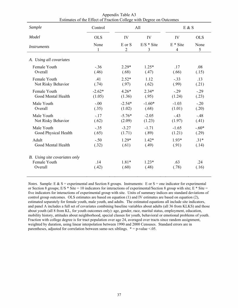
changed in response to the MTO intervention.5 We measure the poverty rate as the average

poverty rate across all addresses at which the household head has resided since random

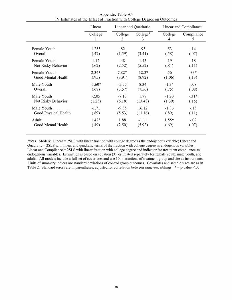
5 In appendix tables A3 and A4 we show that the results are similar using fraction of college graduates as an alternative measure of neighborhood quality. We have also obtained similar results using the census tract share of households that are female-headed and the median family income.

7

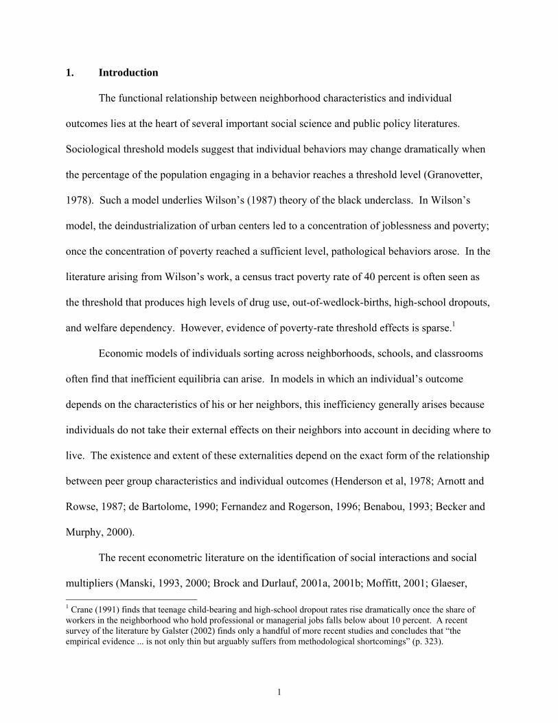
assignment, weighted by the duration of residence.6 Figure 1 shows kernel density estimates of

the distribution of neighborhood poverty rates, with a panel for all sites pooled, and separate

panels for each of the five MTO sites.

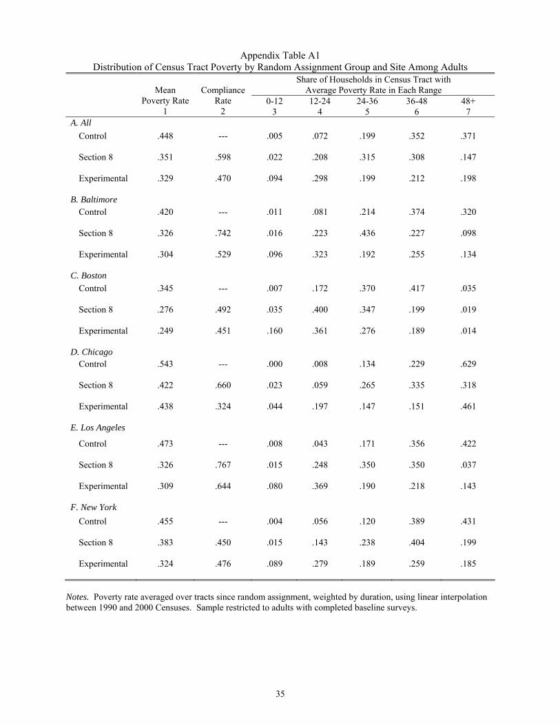
A key feature of MTO mobility patterns – one that we exploit in this paper – is that they

varied considerably by site. In Boston, the average poverty rate for experimental group

households was 10 percentage points lower and for Section 8 group households was seven

percentage points lower than that for control group households. In Los Angeles, by contrast,

average poverty rates were 16 percentage points lower in the experimental group and 15

percentage points lower in the Section 8 group (compared to the control group). Appendix Table

A1 shows these average rates, and summarizes the distribution of census tract poverty rates by

treatment group and site.

In all sites, there is a similar pattern, in which the experimental group has the most

density in low-poverty areas, the Section 8 group has the most density in mid-poverty areas, and

the control group has the most density in high-poverty areas. Many more experimental group

households live in less-disadvantaged areas (39 percent with average tract poverty rates below

24), compared with the Section 8 group (23 percent), and the control group (8 percent). For the

entire control group, the mean poverty rate is 45 percent, compared with 35 percent for the

Section 8 group and 33 percent for the experimental group.

The distributions of duration-weighted average poverty rates in MTO reflect three

underlying patterns. First, not all treatment group families used program-provided Section 8

vouchers to move. The compliance rate – the share of families who moved to new apartments

using vouchers obtained through the program – was 60 percent for the Section 8 group and 47

6 The addresses come from various sources, including surveys in 1997, 2000, and 2002; housing authority records; postal address changes; and credit bureau data.

8

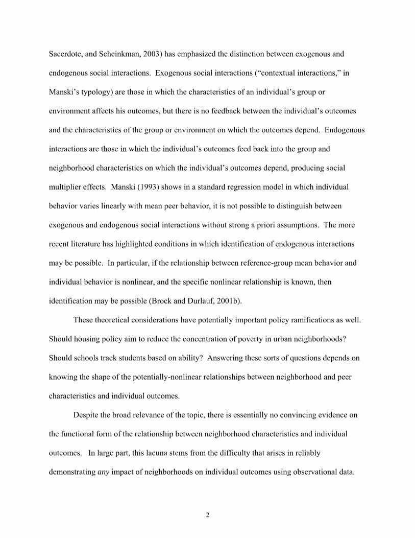
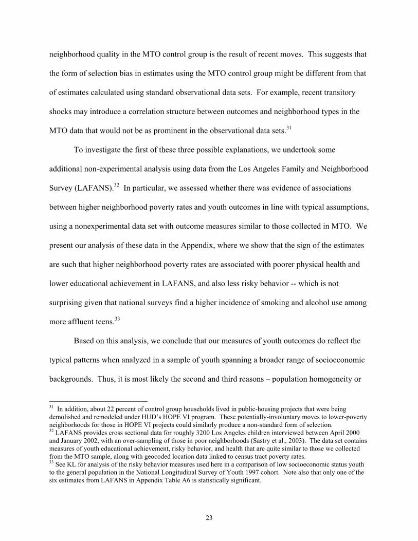
percent for the experimental group. Figure 2 shows kernel density estimates of average poverty

rates by treatment group and compliance status. For experimental group compliers, the mode of

the distribution is 14 percent. For Section 8 group compliers it is 30 percent. The distributions

for the control group as a whole and for noncompliers from each of the treatment groups are

quite similar – all have modes of 46 percent. Thus, the differences in neighborhood poverty

distributions between the treatment groups and the control group are driven by those making

program moves (the compliers).

Second, there was a substantial amount of residential mobility in the sample beyond the

initial program moves. 64 percent of treatment group compliers subsequently moved again after

their initial program move.7 Similar fractions of treatment group noncompliers (62 percent) and

control group members (69 percent) also have moved since random assignment.8

Third, the characteristics of the census tracts to which compliers moved were changing.

The average poverty rate of the tracts to which experimental group households moved rose

significantly from 1990 to 2000. Our duration-weighted average poverty measure uses annual

poverty rates linearly interpolated from the poverty rates of the 1990 and 2000 censuses.

C. Summary indices of youth and adult outcomes

Residential moves with housing vouchers through MTO led families to areas with not

only lower poverty rates but also improved housing, neighborhood conditions, and safety

(KLKS). Experimental and Section 8 families expressed greater satisfaction with their housing

and neighborhoods and indicated much lower criminal victimization rates than control group

families at the time of the interim evaluation survey. These gains in perceived neighborhood

7 The requirement that experimental group families live in a low-poverty neighborhood applied for only one year. Thereafter, they faced no geographic restriction on voucher use. 8 Some were forced to move due to HOPE VI revitalization of their origin housing developments.

9

quality and safety were greater for the experimental families. MTO voucher eligibility did not

have a significant impact on overall adult economic self-sufficiency, but moves to wealthier

neighborhoods were associated with significant improvements in adult mental health and

reductions in adult obesity (KLKS). The impacts of MTO differed substantially for male and

female youth (KL). Teenage girls in both treatment groups experienced improvements in mental

health relative to controls and those in the experimental group experienced reductions in risky

behaviors. Teenage boys in both treatment groups were more likely than controls to engage in

risky behaviors and to experience physical health problems.

In our previous work we have argued that to assess the impacts of this social experiment

it is useful not only to examine specific outcomes (such as test scores or drug use), but also to

construct summary indices that aggregate information across outcomes. We use these summary

measures both to form conclusions about the overall impact of the study and to reduce the

number of statistical tests performed so as to reduce the chance of false positives. In

constructing these summary measures, we express outcomes in standardized units to study mean

effect sizes – in particular, we study the average treatment-control differences across multiple

outcomes, relative to the standard deviation of the control group.

To illustrate the creation of a summary index, the 15 outcomes studied by KL for female

youth ages 15-20 are shown in Table 1.9 Column 1 (labeled “raw”) shows the mean of each

outcome for the control group. In this paper, we focus on normalized transformations of each

outcome (labeled “norm”), where we subtract the mean of the control group and divide by the

standard deviation of the control group.10 In calculating the normed measure, we reverse the

9 The same 15 outcomes for male youth, and five mental health outcomes for adults, are shown in Appendix Table A2. 10 Let Yk be the kth of K outcomes, µk be the control group mean, and σk be the control group standard deviation. The normalized outcome is Yk* = (Yk - µk )/σk. The summary index is Y* = Σk Yk*/K.

10

sign for all outcomes except education, so that a higher value of the normalized measure

represents a more “beneficial” outcome. For alcohol use, the fraction using in the past 30 days

was .22 in the control group and .15 in the experimental group, for an experimental-control (E-

C) difference of -.07 as shown in column 3. This was a difference of .17 standard deviations,

relative to the control group. For depression, the fraction ever having major depression was .14

in the control group, with an E-C difference of -.06. This is also a difference of .17 standard

deviations, relative to the control group. This illustrates how we use this normalization in order

to translate the magnitudes of different measures into standardized units. The bottom row of

Table 1 shows our summary index, which is the equally weighted average of the normalized

transformations for each outcome.11 For all but one of the fifteen outcomes (the exception being

“overall health fair or poor”), the experimental group shows more beneficial outcomes than the

control group, and the E-C difference for our summary index is .11 standard deviations.

In this paper we limit our analysis to summary measures with evidence of statistically

significant treatment effects from the offer of an MTO voucher, since there is little value in

studying the form of the relationship between neighborhood characteristics and outcomes for

outcomes which show no evidence of being affected by neighborhood characteristics.12 Hence,

11 In KL and KLKS we estimate 15 treatment effects simultaneously and work with the mean of these estimates. We refer to these mean effect sizes as “summary measures” that directly summarize the estimates for individual outcomes. In this paper, we simplify matters by creating one variable that is the average of the normalized outcomes, imputing missing values at the mean for each random assignment group when an individual has valid data for at least one outcome. We refer to this as the “summary index” variable. When there is no covariate adjustment in the analysis, as in Table 1, the results using the methods in KL and KLKS are equivalent to the method used in this paper. Small differences between the results reported in this paper and those in KL and KLKS are due to simplifications in the handling of covariates, weights, and missing data. Our “summary index” variable has a value for each individual, whereas the “summary measure” used in KL and KLKS is calculated by combining separate estimates of treatment effects for each outcome. 12 Specifically, we selected all of the summary measures in KL and KLKS with per-comparison p-values below .05. If the relationship between the poverty rate and an outcome were non-monotonic – for example if rates of depression initially fall as people move to slightly lower-poverty neighborhoods and then rise as they continue to live in very low-poverty neighborhoods (possibly due to isolation) – it would be possible to find a statistically significant nonlinear relationship between an outcome and the poverty rate, even if the experimental ITT estimate were zero. In practice, we have repeated the analysis presented in this paper for the full set of statistically insignificant primary

11

we present youth results for female overall, female risky behavior, female mental health, male

overall, male risky behavior, and male physical health – all of which had significant treatment

effects on summary measures in KL.13 For adults, we present results for mental health, the only

summary measure with statistically significant impact estimates in KLKS.14

3. Econometric Analysis

A. OLS estimates

We first explore the importance of neighborhood effects on a range of socioeconomic and

health outcomes for our MTO sample of individuals (indexed by i) living in five major

metropolitan areas (sites indexed by j) using non-experimental variation as a point of departure.

These results are meant to illustrate the approach commonly taken in the non-experimental

neighborhood-effects literature. In a simple regression framework, the most direct test of

theories of neighborhood effects would examine the coefficient vector (γ) in a regression of the

outcome of interest (Y) on a set of observed neighborhood characteristics (W), conditioning on

controls for individual background variables (X) and for metropolitan area fixed effects (δj):

(1) Yij = Wijγ + Xijβ + δj + εij

In Table 2, we follow a large literature (e.g., Wilson, 1987; Jargowsky and Bane, 1990;

Jargowsky, 1997) in using census tract as our neighborhood construct and the poverty rate as our

measure of neighborhood quality (W).15 We interpret the poverty rate as an index for a bundle

outcomes in the MTO interim evaluation study and do not find any instances in which outcomes with insignificant ITT estimates had significant coefficients using the methods we apply in this paper. 13 As shown in Table 1, the overall summary index includes education, risky behavior, mental health, and physical health. The youth risky behavior summary index is the mean for marijuana use, cigarette use, alcohol use, and pregnancy; the youth mental health summary index is the mean for psychological distress, depression, and anxiety; and the youth physical health summary index is the mean for general health, asthma, injuries, and obesity. 14 The adult mental health summary index consists of psychological distress, depression, (lack of) calmness, anxiety, and too little or too much sleep. 15 Although neighborhood variables measured at the census-tract level may not correspond to the ideal neighborhood

12

of correlated characteristics of neighborhoods that are relatively stable, including income levels,

education levels, occupations, etc.; we do not interpret our model as holding these fixed while

the poverty rates vary.16

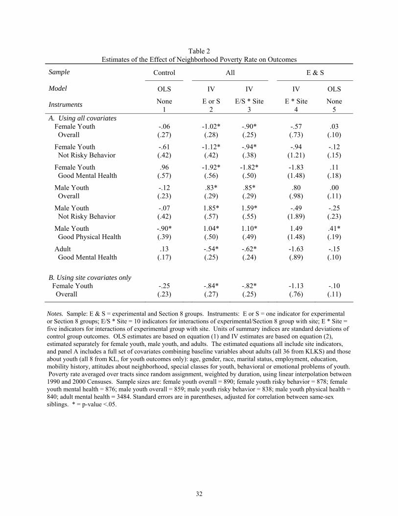
The results in column 1 of Table 2 show OLS estimates of the coefficient γ in equation

(1) for the control group, which did not receive housing vouchers via MTO. With the exception

of male physical health, there are no significant associations between tract poverty and

individual outcomes. The magnitudes of four of the seven OLS control group point estimates are

quite small. For example, the E-C difference in the tract poverty rate was about -.12, and the E-

C difference in the female youth overall index (shown in Table 1) was .11 standard deviations.

Using the results for the control group in column 1 of Table 1, a -.12 change in tract poverty

would be predicted to produce a .007 standard deviation change (-.12 × -.06) in the female

overall index. Thus, the OLS estimate predicts much smaller neighborhood effects than were

actually observed in the MTO experiment for the female youth overall index.

As an alternative non-experimental analysis, one could look at the non-experimental

association between neighborhood poverty and outcomes in the treatment groups. In column 5

concept, we believe that the census tract is the best neighborhood unit available in our data. We focus mainly on the duration-weighted average poverty rate over all residential locations since random assignment. However, we recognize that this need not be the correct functional form for aggregating poverty rates across time; for example it might be the worst or best neighborhood to which an individual is exposed that influences outcomes. Another justification for using the poverty rate as our neighborhood quality measure is that the tract poverty rate is often the focus of policy discussions and has often been used in theoretical models of possible nonlinear and threshold effects of neighborhood quality on outcomes. In Appendix Tables A3 and A4, we present a parallel analysis for tract fraction with a college degree, which is more sensitive to the amount of affluence in the census tract than the poverty rate, which focuses on the more-disadvantaged. In additional analyses not included in this paper, we have found that results are qualitatively similar for a wide range of neighborhood quality measures including share of households that are female-headed and median family income. 16 Even under this less restrictive interpretation, threats to validity of this approach can arise from heterogeneity in treatment effects across sites being driven by factors other than differences in group poverty distributions (such as temporary fluctuations in labor market conditions or differences in the types of families able to take advantage of vouchers and move) that are not stable characteristics of neighborhoods.

13

of Table 2, we see that the OLS estimates of these relationships are also quite small in absolute

value and mostly statistically insignificant.17

B. Instrumental variables estimates of linear models

Non-experimental estimates of equation (1) are unlikely to provide convincing estimates

of the causal effects of neighborhood attributes on outcomes. Most prominently, the selection

problem arising from the systematic sorting of individuals across residential neighborhoods on

the basis of important unobserved determinants of outcomes may lead to severely biased

estimates. The MTO intervention, by inducing exogenous differences between the residential

neighborhoods of the treatment groups and those of the control group, provides a solution to the

problem of the non-random selection of households into different neighborhoods that potentially

confounds estimation of equation (1).

Continuing to use the poverty rate as an index of the bundle of attributes that make up

neighborhood quality, equation (2) uses the offer of an MTO voucher as an instrumental variable

for the poverty rate. Let Z be a set of instrumental variables, and let PZ be the projection matrix

Z(Z’Z)-1Z’. The instrumental variables estimate of equation (1) with the instrument vector Z can

be represented by the regression:

(2) PZYij = PZ(Wijγ + Xijβ + δj + εij)

When Z contains Xij, δj, and a single indicator variable for being assigned to a treatment group

(either experimental or Section 8) as the excluded instrument, then γ is the difference in

outcomes between the treatment and control groups divided by the difference in poverty rates

between the treatment and control groups (after regression adjustment of each difference for X

17 We return to discuss these nonexperimental estimates in further detail after we have presented the instrumental variables results.

14

and δ). Results for this model with one endogenous variable and one instrument are shown in

column 2 of Table 2. For the female overall summary index in panel A, the effect of a .12

change in poverty is estimated to be a .12 standard deviation change in the index – a result which

is quite similar to the .11 observed E-C difference in the index from Table 1.

Using a single indicator to identify the effect of the poverty rate on outcomes essentially

uses two differences in means (one difference in poverty rates, and one difference in outcomes)

as the source of identification, and therefore provides little information about the exact form of

the relationship and about the appropriateness of the linearity assumption. We attempt to

provide some information about the form of this relationship by using multiple instruments. We

first illustrate our approach using a version of equation (2) in which X is dropped from the model

and Z contains the site fixed effects (δ) and a set of ten site-by-treatment group indicators as the

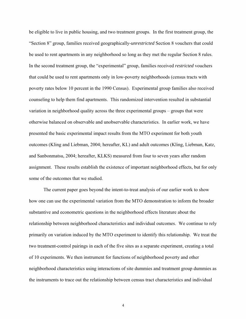
excluded instruments.18 In this case, the projection into the space spanned by Z implies that the

regression slope is fit through the fifteen site-by-random-assignment group means, with each

overall site normalized by the site fixed effects to have mean zero. This is shown graphically in

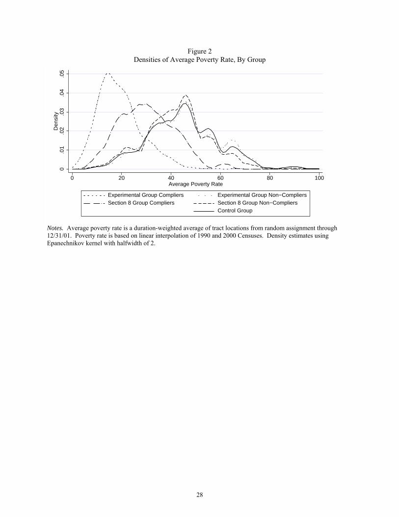
18 In choosing which baseline characteristics to interact with random assignment (RA) group to form a set of instruments, our goal was to produce as much variation as possible with a relatively parsimonious set of instruments so as to avoid problems associated with weak instruments. Site-by-RA group produces substantially more variation in poverty than other possible instrument sets such as race-by-RA group or education-by-RA group. In addition, using the site-RA group interactions allows our results to have the intuitive interpretation of regarding the MTO demonstration as 10 different experiments – two at each site. An alternative plausible approach to generating instruments – predicting poverty with a full set of baseline characteristics and interactions of these characteristics with treatment group and then using the predicted poverty rate as the instrument – would not allow for this intuitive interpretation of our IV results. As in equation (1), we interpret the poverty rate as an index for a bundle of correlated characteristics of neighborhoods. Nevertheless, it remains possible that in using site indicators as instruments, the site differences in treatment effects on outcomes could be correlated with effects on average poverty rates but actually be driven by the interaction of the treatments with some other fundamental factors such as racial discrimination or labor market conditions that are operating at the site level and not the neighborhood level. We do not interpret equation (2) as implying that the entire effect of the treatment works though the mechanism of average poverty rate changes, but instead we are attempting to assess the form of the relationship between outcomes and residential locations when projecting the treatment effects into the intuitively understandable metric of poverty rate changes.

15

Figure 3, a partial regression leverage plot (also known as an added-variable plot) for the female

youth overall summary index.19

In this figure, we see that the control groups at each of the five sites have poverty rates

that are above the average for their sites and outcomes that tend to be below average for their

sites. Moreover, Figure 3 demonstrates a pattern of more-beneficial outcomes in treatment-sites

with larger changes in poverty rates (e.g., the experimental group in LA and NY) and less-

beneficial effects with smaller changes in poverty rates (e.g., the Section 8 group in Baltimore

and NY). The slope of the line in Figure 3 is -.82, which is also reported in panel B of table 2 –

showing the results with no covariates other than site dummies.20

A comparison of columns 2 and 3 shows that the results are nearly the same whether one

excluded instrument is used (as in column 2) or ten excluded instruments are used (as in column

3), and formal over-identification tests do not reject the hypothesis that the linear model is

properly specified. Roughly speaking, what this means is that there is no evidence that the slope

of a line connecting the midpoint of the control estimates to the midpoint of the treatment

estimates in Figure 3 is different from the slope of the line fit through all 15 points in Figure 3.

Another way to examine whether there is a relationship between the neighborhood

poverty rate and outcomes (beyond the effect of the voucher offer itself) is to limit the sample to

19 A partial regression leverage plot shows a bivariate relationship between the dependent variable and one of the independent variables by plotting the residuals from regressing the dependent variable on all of the other independent variables against the residuals from regressing the independent variable of interest on all of the other independent variables (Belsley, Kuh, and Welsch, 1980). In our IV context, define MX = (I - X(X’X)-1X’). Figure 3 shows the partial regression leverage plot, MδPZYij = MδPZWijγ + η. We have also used another diagnostic technique for examining the form of the relationship between the outcomes and poverty rates in each group-site – examining augmented partial residual plots, recommended by Mallows (1986) to detect nonlinearity in f(W). This analysis did not find any evidence of nonlinearities in our estimated relationships. 20 With random assignment, the baseline covariates (X) should be independent of the indicators for the assigned group – implying that the regression adjustment of equation (2) should not affect the point estimate of γ when a full set of baseline covariates is added to the model. Although we have moderate-sized samples and there is some survey attrition that could induce a correlation between the covariates and group indicators, the estimates with and without covariates are quite similar in the full sample IV results, consistent with random assignment. This result can be seen in column 3 of table 3 by comparing the female youth overall result in panel A to the result in panel B.

16

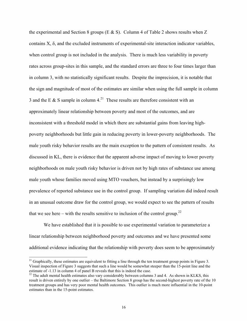
the experimental and Section 8 groups (E & S). Column 4 of Table 2 shows results when Z

contains X, δ, and the excluded instruments of experimental-site interaction indicator variables,

when control group is not included in the analysis. There is much less variability in poverty

rates across group-sites in this sample, and the standard errors are three to four times larger than

in column 3, with no statistically significant results. Despite the imprecision, it is notable that

the sign and magnitude of most of the estimates are similar when using the full sample in column

3 and the E & S sample in column 4.21 These results are therefore consistent with an

approximately linear relationship between poverty and most of the outcomes, and are

inconsistent with a threshold model in which there are substantial gains from leaving high-

poverty neighborhoods but little gain in reducing poverty in lower-poverty neighborhoods. The

male youth risky behavior results are the main exception to the pattern of consistent results. As

discussed in KL, there is evidence that the apparent adverse impact of moving to lower poverty

neighborhoods on male youth risky behavior is driven not by high rates of substance use among

male youth whose families moved using MTO vouchers, but instead by a surprisingly low

prevalence of reported substance use in the control group. If sampling variation did indeed result

in an unusual outcome draw for the control group, we would expect to see the pattern of results

that we see here – with the results sensitive to inclusion of the control group.22

We have established that it is possible to use experimental variation to parameterize a

linear relationship between neighborhood poverty and outcomes and we have presented some

additional evidence indicating that the relationship with poverty does seem to be approximately

21 Graphically, these estimates are equivalent to fitting a line through the ten treatment group points in Figure 3. Visual inspection of Figure 3 suggests that such a line would be somewhat steeper than the 15-point line and the estimate of -1.13 in column 4 of panel B reveals that this is indeed the case. 22 The adult mental health estimates also vary considerably between columns 3 and 4. As shown in KLKS, this result is driven entirely by one outlier – the Baltimore Section 8 group has the second-highest poverty rate of the 10 treatment groups and has very poor mental health outcomes. This outlier is much more influential in the 10-point estimates than in the 15-point estimates.

17

linear for most of the outcomes we study. We next explore the possibility of using experimental

variation to estimate potentially nonlinear relationships between poverty and outcomes.

C. Instrumental variables estimates of nonlinear and threshold models

In equation (3), f(Wij) is a function of the neighborhood characteristics.

(3) PZYij = PZ(f(Wij)γ + Xijβ + δj + εij)

If f(Wij) is nonlinear, then differences in the neighborhood poverty distributions among treatment

groups by site (beyond mean differences) can potentially be used to identify any nonlinear

effects of neighborhood poverty on outcomes. For example, although the mean neighborhood

poverty rates for the experimental and Section 8 groups are almost identical, the underlying

distributions shown in Figure 1 differ substantially.

Table 3 presents estimates from two models where f(W) is a more flexible function of

residential location. The first column repeats the linear IV estimates from column 3 of table 2 to

allow easy comparison with those results. Columns 2 and 3 show coefficients from a model in

which f(W) is assumed to be quadratic. Specifically, poverty and poverty-squared are the two

endogenous variables in W and there are ten site-group interactions used as excluded instruments

in Z. It turns out that we do not have enough precision to estimate the quadratic model – the

standard errors on both coefficients are so large that the estimates are not informative.

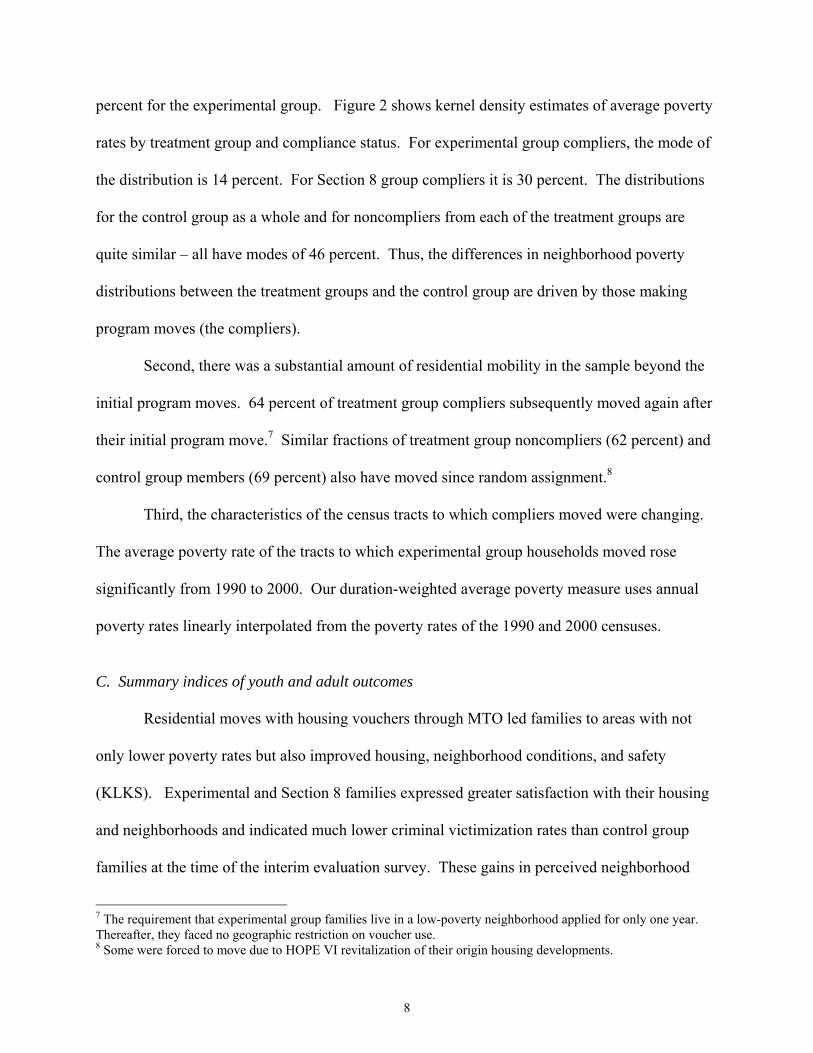
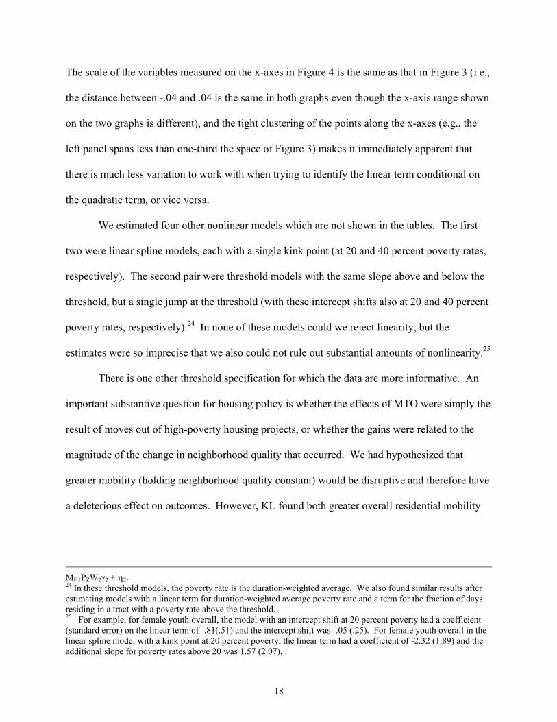
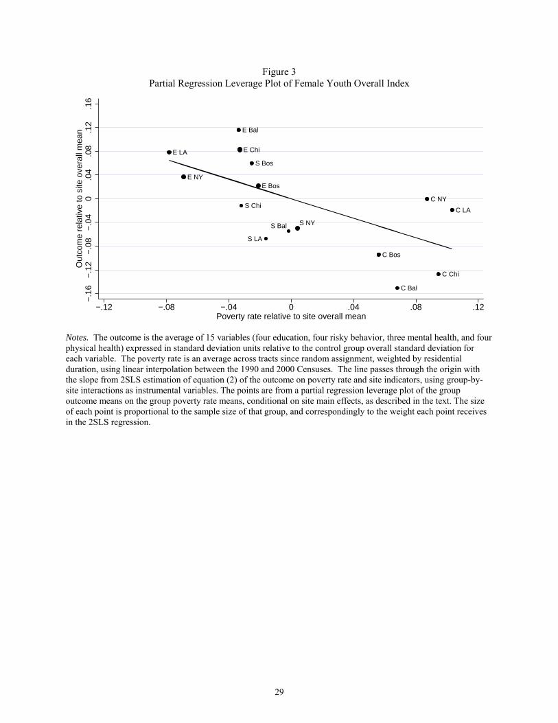
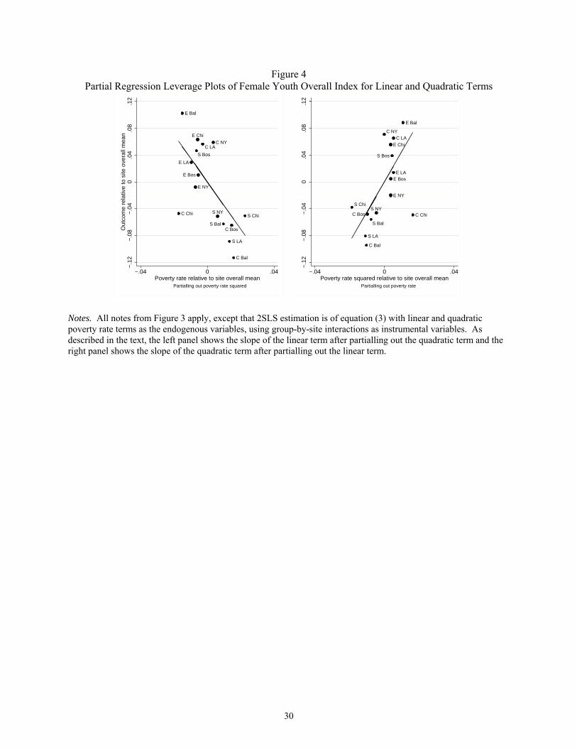
Intuitively, the explanation for this can be seen in figure 4, which is constructed to be analogous

to figure 3 – the left panel is the partial regression leverage plot for the linear term (holding the

quadratic term and the site indicators constant) and the right panel is the partial regression

leverage plot for the quadratic term (holding the linear term and the site indicators constant).23

23 As in figure 3, X is dropped from the model. Let W1 = poverty rate; W2 = poverty rate squared; H1 = [δ : PZW1]; H2 = [δ : PZW2]. Then left panel shows MH2PZYij = MH2PZW1γ1 + η1, and the right panel shows MH1PZYij =

18

The scale of the variables measured on the x-axes in Figure 4 is the same as that in Figure 3 (i.e.,

the distance between -.04 and .04 is the same in both graphs even though the x-axis range shown

on the two graphs is different), and the tight clustering of the points along the x-axes (e.g., the

left panel spans less than one-third the space of Figure 3) makes it immediately apparent that

there is much less variation to work with when trying to identify the linear term conditional on

the quadratic term, or vice versa.

We estimated four other nonlinear models which are not shown in the tables. The first

two were linear spline models, each with a single kink point (at 20 and 40 percent poverty rates,

respectively). The second pair were threshold models with the same slope above and below the

threshold, but a single jump at the threshold (with these intercept shifts also at 20 and 40 percent

poverty rates, respectively).24 In none of these models could we reject linearity, but the

estimates were so imprecise that we also could not rule out substantial amounts of nonlinearity.25

There is one other threshold specification for which the data are more informative. An

important substantive question for housing policy is whether the effects of MTO were simply the

result of moves out of high-poverty housing projects, or whether the gains were related to the

magnitude of the change in neighborhood quality that occurred. We had hypothesized that

greater mobility (holding neighborhood quality constant) would be disruptive and therefore have

a deleterious effect on outcomes. However, KL found both greater overall residential mobility

MH1PZW2γ2 + η2. 24 In these threshold models, the poverty rate is the duration-weighted average. We also found similar results after estimating models with a linear term for duration-weighted average poverty rate and a term for the fraction of days residing in a tract with a poverty rate above the threshold. 25 For example, for female youth overall, the model with an intercept shift at 20 percent poverty had a coefficient (standard error) on the linear term of -.81(.51) and the intercept shift was -.05 (.25). For female youth overall in the linear spline model with a kink point at 20 percent poverty, the linear term had a coefficient of -2.32 (1.89) and the additional slope for poverty rates above 20 was 1.57 (2.07).

19

and more beneficial treatment effects for female youth than for male youth, which was at odds

with this hypothesis.

Equation (3) allows for a straightforward test of this pure threshold model (compared to a

linear model) in the specification where f(W) has a linear term in the poverty rate and an

indicator for compliance (use of an MTO voucher). Columns 4 and 5 of table 3 show estimates

using equation (3), again with ten group-site indicators as excluded instruments and a full set of

covariates. If all of the effects were simply the result of moving out of housing projects, we

would expect to see a zero coefficient on the poverty term and a significant coefficient on the

threshold term. In contrast, if the effect operates primarily through the poverty rate, we would

expect to see a coefficient on the linear term that is similar to that in the simple linear IV

specification.

For the majority of our outcomes, the coefficient on the linear poverty term in this model

with compliance is quite similar to the coefficient in the simple linear IV model (for male youth

overall, male youth physical health, and adult mental health the coefficient in column 4 has

substantially greater magnitude). None of the compliance estimates are statistically significant.

Indeed, for all of the outcomes but one, the point estimates are either very close to zero or are

moderately large but in the wrong direction.26 Interestingly, the linear term for male youth

overall shows a large and significant adverse effect of lower poverty rates. Combined with the

results in Table 2 that show similarity in the magnitude of the results for the full sample and the

E & S sample, this provides some evidence that there was an adverse effect of lower poverty

26 To get a sense of the relative magnitudes of the poverty term and the compliance term, consider a 26 percentage point reduction in poverty, which is the average reduction in duration-weighted poverty for an experimental group complier relative to the control group (for female youth). For the female youth overall result, the poverty coefficient of -1.00 implies that the .26 decrease in neighborhood poverty rates for experimental compliers is associated with a .26 improvement in overall outcomes. The compliance point estimate is -.02, implying that moving out of the housing projects leads to slightly worse outcomes.

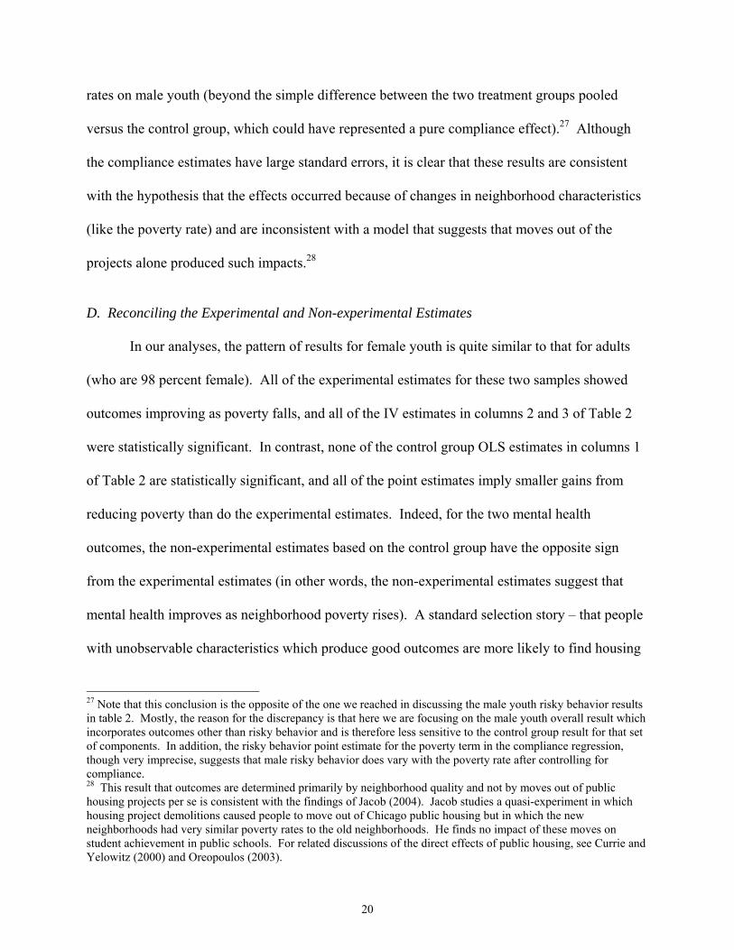
20

rates on male youth (beyond the simple difference between the two treatment groups pooled

versus the control group, which could have represented a pure compliance effect).27 Although

the compliance estimates have large standard errors, it is clear that these results are consistent

with the hypothesis that the effects occurred because of changes in neighborhood characteristics

(like the poverty rate) and are inconsistent with a model that suggests that moves out of the

projects alone produced such impacts.28

D. Reconciling the Experimental and Non-experimental Estimates

In our analyses, the pattern of results for female youth is quite similar to that for adults

(who are 98 percent female). All of the experimental estimates for these two samples showed

outcomes improving as poverty falls, and all of the IV estimates in columns 2 and 3 of Table 2

were statistically significant. In contrast, none of the control group OLS estimates in columns 1

of Table 2 are statistically significant, and all of the point estimates imply smaller gains from

reducing poverty than do the experimental estimates. Indeed, for the two mental health

outcomes, the non-experimental estimates based on the control group have the opposite sign

from the experimental estimates (in other words, the non-experimental estimates suggest that

mental health improves as neighborhood poverty rises). A standard selection story – that people

with unobservable characteristics which produce good outcomes are more likely to find housing

27 Note that this conclusion is the opposite of the one we reached in discussing the male youth risky behavior results in table 2. Mostly, the reason for the discrepancy is that here we are focusing on the male youth overall result which incorporates outcomes other than risky behavior and is therefore less sensitive to the control group result for that set of components. In addition, the risky behavior point estimate for the poverty term in the compliance regression, though very imprecise, suggests that male risky behavior does vary with the poverty rate after controlling for compliance. 28 This result that outcomes are determined primarily by neighborhood quality and not by moves out of public housing projects per se is consistent with the findings of Jacob (2004). Jacob studies a quasi-experiment in which housing project demolitions caused people to move out of Chicago public housing but in which the new neighborhoods had very similar poverty rates to the old neighborhoods. He finds no impact of these moves on student achievement in public schools. For related discussions of the direct effects of public housing, see Currie and Yelowitz (2000) and Oreopoulos (2003).

21

in low-poverty neighborhoods – would have the opposite pattern; in the standard case, the non-

experimental estimates would show greater gains from reducing poverty than would the

experimental estimates.

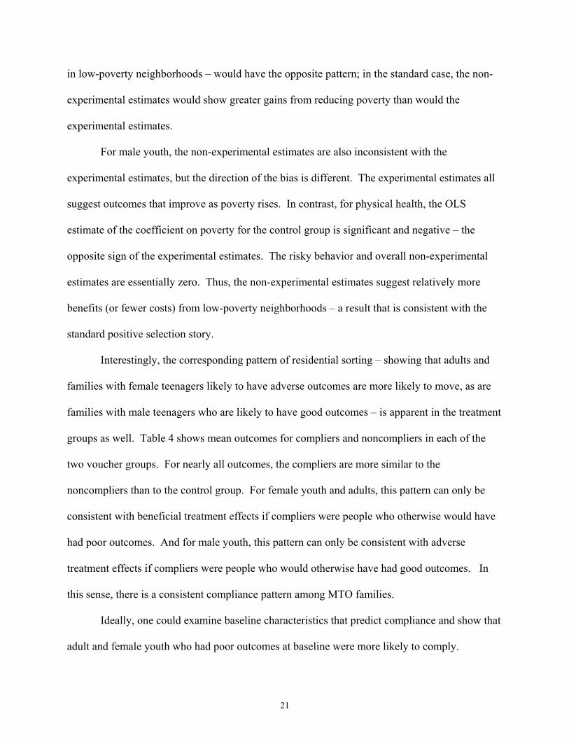
For male youth, the non-experimental estimates are also inconsistent with the

experimental estimates, but the direction of the bias is different. The experimental estimates all

suggest outcomes that improve as poverty rises. In contrast, for physical health, the OLS

estimate of the coefficient on poverty for the control group is significant and negative – the

opposite sign of the experimental estimates. The risky behavior and overall non-experimental

estimates are essentially zero. Thus, the non-experimental estimates suggest relatively more

benefits (or fewer costs) from low-poverty neighborhoods – a result that is consistent with the

standard positive selection story.

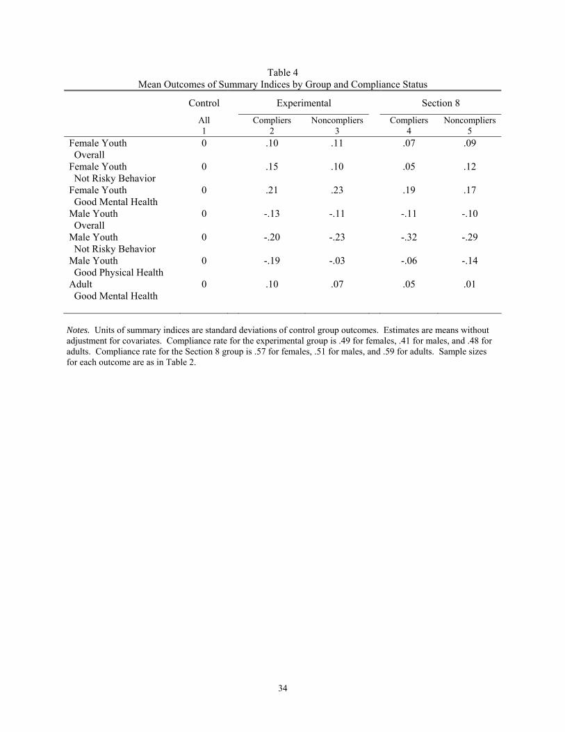
Interestingly, the corresponding pattern of residential sorting – showing that adults and

families with female teenagers likely to have adverse outcomes are more likely to move, as are

families with male teenagers who are likely to have good outcomes – is apparent in the treatment

groups as well. Table 4 shows mean outcomes for compliers and noncompliers in each of the

two voucher groups. For nearly all outcomes, the compliers are more similar to the

noncompliers than to the control group. For female youth and adults, this pattern can only be

consistent with beneficial treatment effects if compliers were people who otherwise would have

had poor outcomes. And for male youth, this pattern can only be consistent with adverse

treatment effects if compliers were people who would otherwise have had good outcomes. In

this sense, there is a consistent compliance pattern among MTO families.

Ideally, one could examine baseline characteristics that predict compliance and show that

adult and female youth who had poor outcomes at baseline were more likely to comply.

22

Unfortunately, our baseline data do not include measures of the main outcomes showing

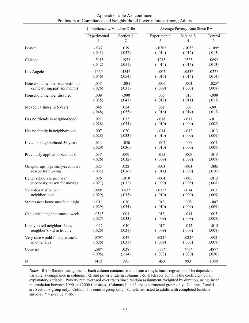
experimental impacts. We have examined the predictors of compliance and of average tract

poverty rate separately for each group (with results shown in Appendix Table A5). Consistent

predictors of greater compliance include younger adult age, smaller household size, and

dissatisfaction with original neighborhood.29 No characteristics except site were consistent

predictors of poverty rates across all three of the groups. Unfortunately, none of these predictors

shed much light on the selection pattern. We do not find any notable differences in the

predictors of compliance between families with male youth and families with female youth –

something that would help explain the different patterns of selection.30

There are several possible explanations for why our non-experimental estimates do not

show evidence of upward bias (for outcomes whose prevalence increases with poverty) from

non-random sorting of households across neighborhoods, as would occur under a typical

assumption that people with positive unobservable characteristics will have good outcomes and

choose to live in better (lower-poverty) neighborhoods. First, it is possible that typical

assumptions about the relationship between neighborhood poverty and outcomes do not hold

among youth for our measures. Second, because the MTO population is relatively homogenous

– consisting almost entirely of minority single mother households originally living in some of the

highest poverty inner city neighborhoods in the country -- the magnitude of selection on

unobservable characteristics may be less than in a standard data set with more heterogeneity.

Third, in typical observational data sets, current variation in neighborhoods is the result of

mobility choices that have occurred over an extended period of time. In contrast, the variation in 29 Entered alone, people who are employed are more likely to move to low-poverty neighborhoods, but this effect drops out once the other predictors are included. 30 An alternative approach to studying this issue would be to estimate a full structural model of neighborhood choice and outcomes conditional on choice. Because our predictors of compliance and poverty rate explained so little of the variation in these measures of mobility and neighborhood choice, we did not pursue this approach.

23

neighborhood quality in the MTO control group is the result of recent moves. This suggests that

the form of selection bias in estimates using the MTO control group might be different from that

of estimates calculated using standard observational data sets. For example, recent transitory

shocks may introduce a correlation structure between outcomes and neighborhood types in the

MTO data that would not be as prominent in the observational data sets.31

To investigate the first of these three possible explanations, we undertook some

additional non-experimental analysis using data from the Los Angeles Family and Neighborhood

Survey (LAFANS).32 In particular, we assessed whether there was evidence of associations

between higher neighborhood poverty rates and youth outcomes in line with typical assumptions,

using a nonexperimental data set with outcome measures similar to those collected in MTO. We

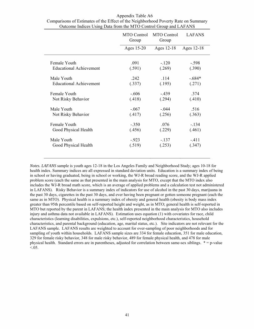
present our analysis of these data in the Appendix, where we show that the sign of the estimates

are such that higher neighborhood poverty rates are associated with poorer physical health and

lower educational achievement in LAFANS, and also less risky behavior -- which is not

surprising given that national surveys find a higher incidence of smoking and alcohol use among

more affluent teens.33

Based on this analysis, we conclude that our measures of youth outcomes do reflect the

typical patterns when analyzed in a sample of youth spanning a broader range of socioeconomic

backgrounds. Thus, it is most likely the second and third reasons – population homogeneity or

31 In addition, about 22 percent of control group households lived in public-housing projects that were being demolished and remodeled under HUD’s HOPE VI program. These potentially-involuntary moves to lower-poverty neighborhoods for those in HOPE VI projects could similarly produce a non-standard form of selection. 32 LAFANS provides cross sectional data for roughly 3200 Los Angeles children interviewed between April 2000 and January 2002, with an over-sampling of those in poor neighborhoods (Sastry et al., 2003). The data set contains measures of youth educational achievement, risky behavior, and health that are quite similar to those we collected from the MTO sample, along with geocoded location data linked to census tract poverty rates. 33 See KL for analysis of the risky behavior measures used here in a comparison of low socioeconomic status youth to the general population in the National Longitudinal Survey of Youth 1997 cohort. Note also that only one of the six estimates from LAFANS in Appendix Table A6 is statistically significant.

24

difference in mobility patterns – that explain why the relationship of youth outcomes and

neighborhood poverty for the MTO control group does not exhibit the pattern typically found in

non-experimental estimates.

4. Conclusion

In this paper, we have shown that it is possible to use the experimental variation from the

Moving to Opportunity experiment to estimate the relationship between neighborhood poverty

and individual outcomes. We have also shown that estimates using non-experimental

approaches are not at all consistent with those from the experimental approach, casting doubt on

the validity of the nonexperimental estimates. Furthermore, the selection patterns necessary to

reconcile the experimental and non-experimental results are complex and differ across

population subgroups, suggesting that it will not in general be possible to identify the direction

of the bias in non-experimental estimates.

Although our estimates of nonlinear and threshold models are not precise enough to be

strongly conclusive, the overall pattern of our results suggests little, if any, deviation from

linearity. We emphasized in the introduction that several important social science and public

policy literatures hinge on knowing the exact functional relationship between neighborhood

characteristics and individual outcomes. Given the unreliability of non-experimental estimates

and the lack of precision in our nonlinear specifications using experimental variation, we are

pessimistic about the prospects for learning more about this question in the immediate future.

But for theorists and policy makers who must make do with the best current evidence, our

recommendation is to assume a linear relationship between poverty and individual outcomes.

25

References

Arnott, Richard and John Rowse. “Peer Group Effects and Educational Attainment.” Journal of Public Economics 32 (1987), 287-305.

Belsley, D.A., E. Kuh, and R.E. Welsch. Regression Diagnostics. New York: John Wiley & Sons, 2000.

Benabou, Roland. “Workings of a City: Location, Education, and Production.” Quarterly Journal of Economics 107 (August 1993), 619-652.

Becker, Gary S. and Kevin M. Murphy. Social Economics. Cambridge, MA: Belknap Press of Harvard University Press, 2000.

de Bartolome, Charles. “Equilibrium and Inefficiency in a Community Model with Peer Effects.” Journal of Political Economy 98 (February 1990), 110-133.

Brock, William A. and Steven N. Durlauf. “Interactions-Based Models,” in James J. Heckman and Edward Leamer, eds., Handbook of Econometrics, vol. 5, 2001a.

Brock, William A. and Steven N. Durlauf. “Discrete Choice with Social Interactions.” Review of Economic Studies 68 (2001b), 235-260.

Crane, Jonathan. “The Epidemic Theory of Ghettos and Neighborhood Effects on Dropping Out and Teenage Childbearing.” American Journal of Sociology 96 (1991), 1226-1259.

Currie, Janet and Aaron Yelowitz. “Are Public Housing Projects Good for Kids?” Journal of Public Economics 75 (January 2000), 99-124.

Duncan, Greg J. and Stephen W. Raudenbush. “Neighborhoods and Adolescent Development: How Can We Determine the Links?” In Alan Booth and Ann C. Crouter, eds., Does it Take a Village? Community Effects on Children, Adolescents, and Families. State College, PA: Pennsylvania State University Press, 2001, 105-136.

Fernandez, Raquel and Richard Rogerson. “Income Distribution, Communities and the Quality of Public Education.” Quarterly Journal of Economics 111 (February 1996), 135-164.

Galster, George. “An Economic Efficiency Analysis of Deconcentrating Poverty Populations.” Journal of Housing Economics 11 (2002), 303-329.

Goering, John and Judith D. Feins, eds. Choosing a Better Life: Evaluating the Moving to Opportunity Social Experiment. Washington, DC: Urban Institute Press, 2003.

Glaeser, Edward L., Bruce A. Sacerdote, and Jose A. Scheinkman. “The Social Multiplier.” Journal of the European Economic Association 1 (April/May 2003), 345-353.

Granovetter, Mark. “Threshold Models of Collective Behavior.” American Journal of Sociology 83 (May 1978), 1420-1443.

Henderson, J. Vernon, Peter Mieszkowski, and Yvon Sauvageau. “Peer Group Effects and Educational Production Functions.” Journal of Public Economics 10 (August 1978), 97-106.

Jacob, Brian A. “Public Housing, Housing Vouchers, and Student Achievement: Evidence from Public Housing Demolitions in Chicago.” American Economic Review 94 (March 2004), 233-258.

26

Jargowsky, Paul A. and Mary Jo Bane. “Ghetto Poverty: Basic Questions.” In L.E. Lynn Jr. and M.G.H. McGeary, eds., Inner-City Poverty in the United States. Washington, DC: National Academy Press, 1990.

Jargowsky, Paul A. Poverty and Place. New York: Russell Sage Foundation, 1997.

Kling, Jeffrey R., Jeffrey B. Liebman, Lawrence F. Katz, and Lisa Sanbonmatsu. “Moving to Opportunity and Tranquility: Neighborhood Effects on Adult Economic Self-Sufficiency and Health from a Randomized Housing Voucher Experiment.” Princeton IRS Working Paper 481, April 2004.

Kling, Jeffrey R. and Jeffrey B. Liebman. “Experimental Analysis of Neighborhood Effects on Youth.” Princeton IRS Working Paper 483, March 2004.

Mallows, C. L. “Augmented Partial Residual Plots.” Technometrics 28 (November 1986), 313-319.

Manski, Charles F. “Identification of Endogenous Social Effects: The Reflection Problem.” Review of Economic Studies 60 (1993), 531-542.

Manski, Chardles F. “Economic Analysis of Social Interactions.” Journal of Economic Perspectives 14 (Summer 2000), 115-136.

Moffitt, Robert. “Policy Interventions, Low-Level Equilibria, and Social Interactions” in Steven N. Durlauf and H. Peyton Young, eds., Social Dynamics (Washington: Brookings Institution), 2001.

Oreopoulos, Philip. “The Long-run Consequences of Growing Up in a Poor Neighborhood,” Quarterly Journal of Economics 118 (November 2003), 1533-1575.

Sastry, Narayan, Bonnie Ghosh-Dastidar, John Adams, Anne R. Pebley. “The Design of a

Multilevel Survey of Children, Families, and Communities: The Los Angeles Family and Neighborhood Survey.” RAND Labor & Population Working Paper Series 03-21, June 2003.

Wilson, William Julius. The Truly Disadvantaged. Chicago: University of Chicago Press, 1987.

27

Figure 1 Densities of Average Poverty Rate, by Site and Group

All sites

0.0

1.0

2.0

3.0

4.0

5D

ensi

ty

0 10 20 30 40 50 60 70 80Average Poverty Rate

Baltimore

0.0

1.0

2.0

3.0

4.0

5D

ensi

ty

0 10 20 30 40 50 60 70 80Average Poverty Rate

ExperimentalSection 8Control

Boston

0.0

1.0

2.0

3.0

4.0

5D

ensi

ty

0 10 20 30 40 50 60 70 80Average Poverty Rate

Chicago

0.0

1.0

2.0

3.0

4.0

5D

ensi

ty

0 10 20 30 40 50 60 70 80Average Poverty Rate

Los Angeles

0.0

1.0

2.0

3.0

4.0

5D

ensi

ty

0 10 20 30 40 50 60 70 80Average Poverty Rate

New York

0.0

1.0

2.0

3.0

4.0

5D

ensi

ty

0 10 20 30 40 50 60 70 80Average Poverty Rate

Notes. Average poverty rate is a duration-weighted average of tract locations from random assignment through 12/31/01. Poverty rate is based on linear interpolation of 1990 and 2000 Censuses. Densities are estimated using an Epanechnikov kernel and a halfwidth of 2.

28

Figure 2 Densities of Average Poverty Rate, By Group

0.0

1.0

2.0

3.0

4.0

5D

ensi

ty

0 20 40 60 80 100Average Poverty Rate

Experimental Group Compliers Experimental Group Non−CompliersSection 8 Group Compliers Section 8 Group Non−Compliers

Control Group

Notes. Average poverty rate is a duration-weighted average of tract locations from random assignment through 12/31/01. Poverty rate is based on linear interpolation of 1990 and 2000 Censuses. Density estimates using Epanechnikov kernel with halfwidth of 2.

29

Figure 3 Partial Regression Leverage Plot of Female Youth Overall Index

E Bal

E Bos

E ChiE LA

E NY

S Bal

S Bos

S Chi

S LA

S NY

C Bal

C Bos

C Chi

C LA

C NY

−.1

6−

.12

−.0

8−

.04

0.0

4.0

8.1

2.1

6O

utco

me

rela

tive

to s

ite o

vera

ll m

ean

−.12 −.08 −.04 0 .04 .08 .12Poverty rate relative to site overall mean

Notes. The outcome is the average of 15 variables (four education, four risky behavior, three mental health, and four physical health) expressed in standard deviation units relative to the control group overall standard deviation for each variable. The poverty rate is an average across tracts since random assignment, weighted by residential duration, using linear interpolation between the 1990 and 2000 Censuses. The line passes through the origin with the slope from 2SLS estimation of equation (2) of the outcome on poverty rate and site indicators, using group-by-site interactions as instrumental variables. The points are from a partial regression leverage plot of the group outcome means on the group poverty rate means, conditional on site main effects, as described in the text. The size of each point is proportional to the sample size of that group, and correspondingly to the weight each point receives in the 2SLS regression.

30

Figure 4 Partial Regression Leverage Plots of Female Youth Overall Index for Linear and Quadratic Terms

E Bal

E Bos

E Chi

E LA

E NY

S Bal

S Bos

S Chi

S LA

S NY

C Bal

C Bos

C Chi

C LAC NY

−.1

2−

.08

−.0

40

.04

.08

.12

Out

com

e re

lativ

e to

site

ove

rall

mea

n

−.04 0 .04Poverty rate relative to site overall mean

Partialling out poverty rate squared

E Bal

E Bos

E Chi

E LA

E NY

S Bal

S Bos

S Chi

S LA

S NY

C Bal

C Bos C Chi

C LAC NY

−.1

2−

.08

−.0

40

.04

.08

.12

−.04 0 .04Poverty rate squared relative to site overall mean

Partialling out poverty rate

Notes. All notes from Figure 3 apply, except that 2SLS estimation is of equation (3) with linear and quadratic poverty rate terms as the endogenous variables, using group-by-site interactions as instrumental variables. As described in the text, the left panel shows the slope of the linear term after partialling out the quadratic term and the right panel shows the slope of the quadratic term after partialling out the linear term.

31

Table 1 Components of Female Overall Index, Means

CM E-C S-C

Raw 1

Norm 2

Raw 3

Norm 4

Raw 5

Norm 6

A. Education

Graduated or in school .79 0 .04 .09 -.00 -.01

In school or working .78 0 .05 .12 -.02 -.05

Reading z-score .08 0 .04 .04 .03 .03

Math z-score .01 0 .11 .13 .08 .09

B. Risky Behavior

Marijuana in past 30 days .12 0 -.05* .15* -.04 .11

Cigarette in past 30 days .18 0 -.05 .12 -.05 .12

Alcohol in past 30 days .22 0 -.07* .17* -.08* .20*

Ever been pregnant .27 0 -.03 .06 .05 -.11

C. Mental health

Distress z-score .28 0 -.29* .26* -.11 .10

Ever had major depression .14 0 -.06* .17* -.06* .18*

Ever had generalized anxiety .14 0 -.08* .23* -.09* .26*

D. Physical health

Overall health fair or poor .10 0 .02 -.06 .02 -.05

Asthma attack in past year .20 0 -.00 .00 -.03 .08

Non-sports injury in past year .12 0 -.03 .09 -.05 .15

Obese .18 0 -.02 .05 -.02 .06

E. Summary index of 15 items 0 .11* .08*

Notes. Raw = unadjusted value. Norm = (unadjusted value - control mean)/(control standard deviation); sign reversed for risky behavior, mental health, and physical health. CM = Control mean. E-C = Experimental - Control. S-C = Section 8 - Control. Differences based on unadjusted means, with no covariates. Summary index is the mean of normalized values of 15 component items. Sample size is 890. * = p-value <.05.

32

Table 2 Estimates of the Effect of Neighborhood Poverty Rate on Outcomes

Sample Control All E & S

Model OLS IV IV IV OLS

Instruments None 1

E or S 2

E/S * Site 3

E * Site 4

None 5

A. Using all covariates Female Youth Overall

-.06 (.27)

-1.02* (.28)

-.90* (.25)

-.57 (.73)

.03 (.10)

Female Youth Not Risky Behavior

-.61 (.42)

-1.12* (.42)

-.94* (.38)

-.94 (1.21)

-.12 (.15)

Female Youth Good Mental Health

.96 (.57)

-1.92* (.56)

-1.82* (.50)

-1.83 (1.48)

.11 (.18)

Male Youth Overall

-.12 (.23)

.83* (.29)

.85* (.29)

.80 (.98)

.00 (.11)

Male Youth Not Risky Behavior

-.07 (.42)

1.85* (.57)

1.59* (.55)

-.49 (1.89)

-.25 (.23)

Male Youth Good Physical Health

-.90* (.39)

1.04* (.50)

1.10* (.49)

1.49 (1.48)

.41* (.19)

Adult Good Mental Health

.13 (.17)

-.54* (.25)

-.62* (.24)

-1.63 (.89)

-.15 (.10)

B. Using site covariates only

Female Youth Overall

-.25 (.23)

-.84* (.27)

-.82* (.25)

-1.13 (.76)

-.10 (.11)

Notes. Sample: E & S = experimental and Section 8 groups. Instruments: E or S = one indicator for experimental or Section 8 groups; E/S * Site = 10 indicators for interactions of experimental/Section 8 group with site; E * Site = five indicators for interactions of experimental group with site. Units of summary indices are standard deviations of control group outcomes. OLS estimates are based on equation (1) and IV estimates are based on equation (2), estimated separately for female youth, male youth, and adults. The estimated equations all include site indicators, and panel A includes a full set of covariates combining baseline variables about adults (all 36 from KLKS) and those about youth (all 8 from KL, for youth outcomes only): age, gender, race, marital status, employment, education, mobility history, attitudes about neighborhood, special classes for youth, behavioral or emotional problems of youth. Poverty rate averaged over tracts since random assignment, weighted by duration, using linear interpolation between 1990 and 2000 Censuses. Sample sizes are: female youth overall = 890; female youth risky behavior = 878; female youth mental health = 876; male youth overall = 859; male youth risky behavior = 838; male youth physical health = 840; adult mental health = 3484. Standard errors are in parentheses, adjusted for correlation between same-sex siblings. * = p-value <.05.

33

Table 3 IV Estimates of the Effect of Neighborhood Poverty Rates on Outcomes

Models Linear Linear and Quadratic Linear and Compliance

Endogenous variables Poverty 1

Poverty 2

Poverty2

3 Poverty

4 Compliance

5

Female Youth Overall

-.90* (.25)

-1.28 (1.19)

.49 (1.51)

-1.00 (.55)

-.02 (.12)

Female Youth Not Risky Behavior

-.94* (.38)

-1.73 (1.87)

1.04 (2.52)

-1.03 (.84)

-.02 (.19)

Female Youth Good Mental Health

-1.82* (.50)

-1.48 (2.14)

-.45 (2.71)

-1.84 (1.08)

-.00 (.25)

Male Youth Overall

.85* (.29)

.02 (1.62)

1.11 (2.20)

1.47* (.68)

.16 (.16)

Male Youth Not Risky Behavior

1.59* (.55)

-1.26 (3.45)

3.79 (4.67)

1.00 (1.36)

-.15 (.33)

Male Youth Good Physical Health

1.10* (.49)

-1.27 (2.51)

3.17 (3.33)

1.93 (1.16)

.21 (.26)

Adult Good Mental Health

-.62* (.24)

-.74 (1.18)

.16 (1.56)

-1.35* (.60)

-.17 (.13)

Notes. Models: Linear = 2SLS with linear poverty rate as the endogenous variable; Linear and Quadratic = 2SLS with linear and quadratic terms of the poverty rate as endogenous variables; Linear and Compliance = 2SLS with linear poverty rate and indicator for treatment compliance as endogenous variables. Estimation is based on equation (3), estimated separately for female youth, male youth, and adults. All models include a full set of covariates and use 10 interactions of treatment group and site as excluded instruments. Units of summary indices are standard deviations of control group outcomes. Covariates and sample sizes are as in Table 2. Standard errors are in parentheses, adjusted for correlation between same-sex siblings. * = p-value <.05.

34

Table 4 Mean Outcomes of Summary Indices by Group and Compliance Status

Control Experimental Section 8

All 1

Compliers 2

Noncompliers 3

Compliers 4

Noncompliers 5

Female Youth Overall

0 .10 .11 .07 .09

Female Youth Not Risky Behavior

0 .15 .10 .05 .12

Female Youth Good Mental Health

0 .21 .23 .19 .17

Male Youth Overall

0 -.13 -.11 -.11 -.10

Male Youth Not Risky Behavior

0 -.20 -.23 -.32 -.29

Male Youth Good Physical Health

0 -.19 -.03 -.06 -.14

Adult Good Mental Health

0 .10 .07 .05 .01

Notes. Units of summary indices are standard deviations of control group outcomes. Estimates are means without adjustment for covariates. Compliance rate for the experimental group is .49 for females, .41 for males, and .48 for adults. Compliance rate for the Section 8 group is .57 for females, .51 for males, and .59 for adults. Sample sizes for each outcome are as in Table 2.

35

Appendix Table A1 Distribution of Census Tract Poverty by Random Assignment Group and Site Among Adults

Share of Households in Census Tract with Average Poverty Rate in Each Range

Mean

Poverty Rate 1

Compliance

Rate 2

0-12 3

12-24 4

24-36 5

36-48 6

48+ 7

A. All Control .448 --- .005 .072 .199 .352 .371

Section 8 .351 .598 .022 .208 .315 .308 .147

Experimental .329 .470 .094 .298 .199 .212 .198

B. Baltimore Control .420 --- .011 .081 .214 .374 .320

Section 8 .326 .742 .016 .223 .436 .227 .098

Experimental .304 .529 .096 .323 .192 .255 .134

C. Boston Control .345 --- .007 .172 .370 .417 .035

Section 8 .276 .492 .035 .400 .347 .199 .019

Experimental .249 .451 .160 .361 .276 .189 .014

D. Chicago Control .543 --- .000 .008 .134 .229 .629

Section 8 .422 .660 .023 .059 .265 .335 .318

Experimental .438 .324 .044 .197 .147 .151 .461

E. Los Angeles

Control .473 --- .008 .043 .171 .356 .422

Section 8 .326 .767 .015 .248 .350 .350 .037

Experimental .309 .644 .080 .369 .190 .218 .143

F. New York Control .455 --- .004 .056 .120 .389 .431

Section 8 .383 .450 .015 .143 .238 .404 .199

Experimental .324 .476 .089 .279 .189 .259 .185

Notes. Poverty rate averaged over tracts since random assignment, weighted by duration, using linear interpolation between 1990 and 2000 Censuses. Sample restricted to adults with completed baseline surveys.

36

Appendix Table A2 Components of Summary Indices for Male Youth and Adults

CM E-C S-C

Raw 1

Norm 2

Raw 3

Norm 4

Raw 5

Norm 6

A. Male youth education

Graduated or in school .76 0 -.04 -.10 -.00 -.01

In school or working .76 0 -.02 -.04 -.03 -.08

Reading z-score -.11 0 -.08 -.07 .10 .08

Math z-score -.03 0 -.14 -.13 -.03 -.03

B. Male youth risky behavior

Marijuana in past 30 days .12 0 .06* -.20* .10* -.30*

Cigarette in past 30 days .13 0 .12* -.35* .15* -.46*

Alcohol in past 30 days .14 0 .06 -.18 .11* -.31*

Ever been pregnant .12 0 .04 -.13 .04 -.13

C. Male youth mental health

Distress z-score -.18 0 .09 -.10 .04 -.05

Ever had major depression .03 0 .01 -.05 .00 -.01

Ever had generalized anxiety .05 0 .01 -.03 -.02 .11

D. Male youth physical health

Overall health fair or poor .06 0 .01 -.04 .00 -.01

Asthma attack in past year .12 0 .03 -.08 .05 -.16

Non-sports injury in past year .07 0 .07* -.28* .07* -.30*

Obese .18 0 -.01 .03 -.03 .07

E. Male youth overall index 0 -.12* -.11*

F. Adult mental health

Distress z-score .05 0 -.09* .09* -.04 .04

Depression in past 12 months .16 0 -.03* .08* -.02 .05

Worrying .39 0 -.02 .05 -.01 .01

Calm and peaceful .46 0 .07* .13* .02 .04

Sleep 7-8 hours nightly .45 0 .04 .07 .02 .03

G. Adult mental health index 0 .08* .03

Notes. Raw = unadjusted value. Norm = (unadjusted value - control mean)/(control standard deviation); sign reversed for risky behavior, mental health, and physical health. CM = Control mean. E-C = Experimental - Control. S-C = Section 8 - Control. Differences based on unadjusted means, with no covariates. Summary index is the mean of normalized values of component items. Sample sizes are 859 and 3484 for male youth and all adults, respectively. * = p-value <.05.

37

Appendix Table A3 Estimates of the Effect of Fraction College with Degree on Outcomes

Sample Control All E & S

Model OLS IV IV IV OLS

Instruments None 1

E or S 2

E/S * Site 3

E * Site 4

None 5

A. Using all covariates

Female Youth Overall

-.36 (.46)

2.29* (.68)

1.25* (.47)

.17 (.66)

.08 (.15)

Female Youth Not Risky Behavior

.41 (.74)

2.52* (.97)

1.12 (.62)

-.33 (.99)

.13 (.21)

Female Youth Good Mental Health

-2.62* (1.05)

4.26* (1.36)

2.34* (.95)

-.29 (1.24)

-.29 (.23)

Male Youth Overall

-.00 (.35)

-2.54* (1.02)

-1.60* (.68)

-1.03 (1.01)

-.20 (.20)

Male Youth Not Risky Behavior

-.17 (.62)

-5.76* (2.09)

-2.05 (1.23)

-.43 (1.97)

-.48 (.41)

Male Youth Good Physical Health

-.35 (.65)

-3.27 (1.71)

-1.71 (.89)

-1.65 (1.21)

-.60* (.29)

Adult Good Mental Health

-.50 (.32)

1.29* (.61)

1.42* (.49)

1.93* (.91)

.31* (.14)

B. Using site covariates only

Female Youth Overall

.14 (.42)

1.81* (.60)

1.23* (.48)

.63 (.78)

.24 (.16)

Notes. Sample: E & S = experimental and Section 8 groups. Instruments: E or S = one indicator for experimental or Section 8 groups; E/S * Site = 10 indicators for interactions of experimental/Section 8 group with site; E * Site = five indicators for interactions of experimental group with site. Units of summary indices are standard deviations of control group outcomes. OLS estimates are based on equation (1) and IV estimates are based on equation (2), estimated separately for female youth, male youth, and adults. The estimated equations all include site indicators, and panel A includes a full set of covariates combining baseline variables about adults (all 36 from KLKS) and those about youth (all 8 from KL, for youth outcomes only): age, gender, race, marital status, employment, education, mobility history, attitudes about neighborhood, special classes for youth, behavioral or emotional problems of youth. Fraction with college degree is for tract population over age 24, averaged over tracts since random assignment, weighted by duration, using linear interpolation between 1990 and 2000 Censuses. Standard errors are in parentheses, adjusted for correlation between same-sex siblings. * = p-value <.05.

38

Appendix Table A4 IV Estimates of the Effect of Fraction with College Degree on Outcomes

Linear Linear and Quadratic Linear and Compliance

College 1

College 2

College2

3 College

4 Compliance

5

Female Youth Overall

1.25* (.47)

.82 (1.59)

.93 (3.41)

.53 (.58)

.14 (.07)

Female Youth Not Risky Behavior

1.12 (.62)

.48 (2.52)

1.45 (5.52)

.19 (.81)

.18 (.11)

Female Youth Good Mental Health

2.34* (.95)

7.82* (3.91)

-12.37 (8.92)

.56 (1.06)

.33* (.13)

Male Youth Overall

-1.60* (.68)

-5.55 (3.57)

8.34 (7.56)

-1.34 (.75)

-.08 (.08)

Male Youth Not Risky Behavior

-2.05 (1.23)

-7.13 (6.18)

1.77 (13.48)

-1.20 (1.39)

-.31* (.15)

Male Youth Good Physical Health

-1.71 (.89)

-9.35 (5.53)

16.12 (11.16)

-1.36 (.89)

-.13 (.11)

Adult Good Mental Health

1.42* (.49)

1.88 (2.50)

-1.11 (5.92)

1.55* (.69)

-.02 (.07)

Notes. Models: Linear = 2SLS with linear fraction with college degree as the endogenous variable; Linear and Quadratic = 2SLS with linear and quadratic terms of the fraction with college degree as endogenous variables; Linear and Compliance = 2SLS with linear fraction with college degree and indicator for treatment compliance as endogenous variables. Estimation is based on equation (3), estimated separately for female youth, male youth, and adults. All models include a full set of covariates and use 10 interactions of treatment group and site as instruments. Units of summary indices are standard deviations of control group outcomes. Covariates and sample sizes are as in Table 2. Standard errors are in parentheses, adjusted for correlation between same-sex siblings. * = p-value <.05.

39

Appendix Table A5 Predictors of Compliance and Neighborhood Poverty Rates Among Adults

Compliance w/Voucher Offer Average Poverty Rate Since RA

Experimental

1 Section 8

2 Experimental

3 Section 8

4 Control

5

Male adult -.174 -.072 .043 .017 -.047

(.122) (.106)

( .041) (.027) (.029)

Adult 0-29 .207* .204* -.054* -.021 .019

(.058) (.069)

( .020) (.018) (.019)

Adult 30-39 .085* .201* -.031* -.022 .003

(.046) (.053)

( .015) (.014) (.015)

Adult 40-49 -.027 .131* .000 -.006 .006

(.045) (.051)

( .015) (.013) (.014)

Adult Hispanic -.005 .009 -.009 .000 -.014

(.051) (.058)

( .017) (.015) (.015)

Adult African-American -.122 -.012 .026 .025 .037

(.063) (.072)

( .021) (.019) (.019)

Adult other non-white -.218* -.024 .060* .017 .023

(.057) (.061)

( .019) (.016) (.017)

Adult never married .001 -.044 .019 .029* .014

(.030) (.036)

( .010) (.009) (.009)

Adult working .032 .058 -.009 -.017 -.007

(.033) (.040)

( .011) (.010) (.010)

Adult was teen parent .019 .064 -.006 -.025* -.009

(.032) (.038)

( .011) (.010) (.010)

Adult in school .086* .052 -.024* -.010 .006

(.036) (.043)

( .012) (.011) (.011)

Adult graduated from high school .051 .022 -.013 -.029* -.009

(.029) (.035)

( .010) (.009) (.009)

Adult obtained GED .103* .060 -.027* -.014 .012

(.037) (.044)

( .013) (.011) (.011)

Core household size equals 1 or 2 .118* .102* -.017 -.005 -.019

(.041) (.048)

( .014) (.012) (.012)

Core household size equals 3 .069 .030 -.021 -.004 -.017

(.036) (.043)

( .012) (.011) (.011)

Core household size equals 4 .062 .062 -.003 -.009 -.014

(.037) (.044)

( .012) (.011) (.011)

No teens in core household .023 .074* -.005 -.013 -.012

(.031) (.037)

( .011) (.010) (.010)

Receiving AFDC/TANF .042 .065 -.008 -.001 -.000

(.035) (.040)

( .012) (.010) (.011)

Has car that runs .042 .026 -.020 -.026* -.019

(.037) (.044)

( .013) (.011) (.012)

Baltimore .003 .239* -.011 -.054* -.042*

(.045) (.054)

( .015) (.014) (.014)

40

Appendix Table A5, continued Predictors of Compliance and Neighborhood Poverty Rates Among Adults

Compliance w/Voucher Offer Average Poverty Rate Since RA

Experimental

1 Section 8

2 Experimental

3 Section 8

4 Control

5

Boston -.047 .039 -.070* -.105* -.109*

(.041) (.047)

( .014) (.012) (.013)

Chicago -.201* .197* .121* .033* .069*

(.042) (.051)

( .014) (.013) (.013)

Los Angeles .133* .354* -.007 -.053* .027*

(.046) (.054)

( .015) (.014) (.014)

Household member was victim of .037 -.004 -.006 -.003 -.025* crime during past six months

(.026) (.031)

( .009) (.008) (.008)

Household member disabled .009 -.000 .005 .013 -.000

(.035) (.041)

( .012) (.011) (.011)

Moved 3+ times in 5 years .045 .054 .001 .007 -.001

(.048) (.055)

( .016) (.014) (.013)

Has no friends in neighborhood .021 .033 -.018 -.011 -.011

(.028) (.034)

( .010) (.009) (.008)

Has no family in neighborhood .007 .020 -.014 -.012 -.013

(.028) (.033)

( .010) (.009) (.009)

Lived in neighborhood 5+ years .014 -.050 -.007 .000 .007

(.029) (.036)

( .010) (.009) (.009)

Previously applied to Section 8 .037 .009 -.015 -.008 -.013

(.026) (.032)

( .009) (.008) (.008)

Gangs/drugs is primary/secondary .025 .022 -.003 -.003 -.005 reason for moving

(.031) (.036)

( .011) (.009) (.010)

Better schools is primary/ .026 -.018 -.004 -.005 -.013 secondary reason for moving

(.027) (.032)

( .009) (.008) (.008)

Very dissatisfied with .090* .083* -.035* -.014 .003 neighborhood

(.029) (.035)

( .010) (.009) (.009)

Streets near home unsafe at night -.016 .020 .013 .008 -.007

(.029) (.034)

( .010) (.009) (.009)

Chats with neighbor once a week -.054* .004 .013 -.014 .005

(.027) (.033)

( .009) (.008) (.008)

Likely to tell neighbor if saw -.042 .040 .017 -.012 -.015 neighbor’s kid in trouble

(.026) (.031)

( .009) (.008) (.008)

Very sure would find apartment .079* .047 -.021* -.022* .002 in other area

(.026) (.031)

( .009) (.008) (.008)

Constant .298* .038 .375* .447* .487* (.098) (.114)

( .033) (.030) (.030)

N 1453 993 1453 993 1080

Notes. RA = Random assignment. Each column contains results from a single linear regression. The dependent variable is compliance in columns 1-2, and poverty rate in columns 3-5. Each row contains the coefficient on an explanatory variable. Poverty rate averaged over tracts since random assignment, weighted by duration, using linear interpolation between 1990 and 2000 Censuses. Columns 1 and 3 are experimental group only. Columns 2 and 4 are Section 8 group only. Column 5 is control group only. Sample restricted to adults with completed baseline surveys. * = p-value < .05.

41

Appendix Table A6 Comparisons of Estimates of the Effect of the Neighborhood Poverty Rate on Summary

Outcome Indices Using Data from the MTO Control Group and LAFANS

MTO Control Group

MTO Control Group

LAFANS

Ages 15-20 Ages 12-18 Ages 12-18

Female Youth Educational Achievement

.091 (.591)

-.120 (.269)

-.598 (.390)

Male Youth Educational Achievement

.242 (.337)

.114 (.195)

-.684* (.271)

Female Youth Not Risky Behavior

-.606 (.418)

-.439 (.294)

.374 (.410)

Male Youth Not Risky Behavior

-.067 (.417)

-.044 (.256)

.516 (.363)

Female Youth Good Physical Health

-.350 (.456)

.076 (.229)

-.134 (.461)

Male Youth Good Physical Health

-.923 (.519)

-.137 (.253)

-.411 (.347)

Notes. LAFANS sample is youth ages 12-18 in the Los Angeles Family and Neighborhood Study; ages 10-18 for health index. Summary indices are all expressed in standard deviation units. Education is a summary index of being in school or having graduated, being in school or working, the WJ-R broad reading score, and the WJ-R applied problem score (each the same as that presented in the main analysis for MTO, except that the MTO index also includes the WJ-R broad math score, which is an average of applied problems and a calculation test not administered in LAFANS). Risky Behavior is a summary index of indicators for use of alcohol in the past 30 days, marijuana in the past 30 days, cigarettes in the past 30 days, and ever having been pregnant or gotten someone pregnant (each the same as in MTO). Physical health is a summary index of obesity and general health (obesity is body mass index greater than 95th percentile based on self-reported height and weight, as in MTO; general health is self-reported in MTO but reported by the parent in LAFANS; the health index presented in the main analysis for MTO also includes injury and asthma data not available in LAFANS). Estimation uses equation (1) with covariates for race, child characteristics (learning disabilities, expulsions, etc.), self-reported neighborhood characteristics, household characteristics, and parental background (education, age, marital status, etc.). Site indicators are not relevant for the LAFANS sample. LAFANS results are weighted to account for over-sampling of poor neighborhoods and for sampling of youth within households. LAFANS sample sizes are 334 for female education, 351 for male education, 329 for female risky behavior, 348 for male risky behavior, 489 for female physical health, and 478 for male physical health. Standard errors are in parentheses, adjusted for correlation between same-sex siblings. * = p-value <.05.

42

Appendix. Non-Experimental Results using LAFANS

This appendix compares nonexperimental estimates using the MTO control group to those from the Los Angeles Family and Neighborhood Study, a data set representative of data sets typically used in nonexperimental analyses of neighborhood effects. Appendix Table A6 contains the results from this nonexperimental analysis.

The LAFANS sample – representative of all youth in LA – lives, on average, in neighborhoods with an average poverty rate of 18 percent, which is much lower than the average rate of 45 percent for the MTO control group. It is typical of datasets used for nonexperimental analyses of neighborhood effects in that it contains a much less homogenous population than MTO, with a much greater proportion of the sample in more affluent areas.

We created outcome variables using LAFANS data similar to those used in our MTO analyses for several domains. The survey items and achievement tests are nearly identical in the two studies. All four measures of youth risky behavior are available in both data sets. For youth health and education, the indices use a subset of the measures in our main MTO analyses that were also available in LAFANS, as detailed in the notes to Appendix Table A6. Because the LAFANS youth sample ranges in age only up to 18, we present LAFANS and MTO estimates for ages 12-18. For MTO we also present results for the ages 15-20 sample that we use in our main MTO analyses of youth outcomes.

Appendix Table A6 shows estimates separately for male and female youth for the domains of educational achievement, absence of risky behavior, and good physical health. Four of the six LAFANS results (those for educational achievement and physical health for both genders) exhibit the “standard” nonexperimental pattern of worse outcomes with higher poverty, though only one of the four is statistically significant. For the risky behavior estimates, we find the opposite pattern: risky behavior falls as poverty rises, though the estimates are not statistically significant. The LAFANS results exhibit no evidence of the gender pattern found in the MTO results using experimental variation, where higher poverty neighborhoods were associated with more adverse outcomes for females but more beneficial outcomes for males.