WORKING PAPER ITLS-WP-14-16 Linking Discrete...

WORKING PAPER

ITLS-WP-14-16

Linking Discrete Choice to Continuous Demand in a Spatial Computable General Equilibrium Model By

Truong P. Truong and David A. Hensher

August 2014

ISSN 1832-570X

INSTITUTE of TRANSPORT and LOGISTICS STUDIES The Australian Key Centre in Transport and Logistics Management

The University of Sydney Established under the Australian Research Council’s Key Centre Program.

NUMBER: Working Paper ITLS-WP-14-16

TITLE: Linking Discrete Choice to Continuous Demand in a Spatial Computable General Equilibrium Model

ABSTRACT: Discrete choice (DC) models are often used to describe consumer behaviour at a disaggregate level where the choice decision is defined in terms of a set of alternatives (commodities) differentiated mainly by their quality attributes rather than just prices, and individuals making the choice decisions are differentiated by their socio-economic characteristics rather than just income level. DC models therefore are rich in details which are important for policies analysis at a micro or intra-sectoral level (e.g., transport sector, housing sector). In contrast, continuous demand (CD) models are specialized in describing behaviour at an aggregate (inter-sectoral) level (e.g. trade-off between transport and land-use activities). DC and CD models are therefore complements rather than substitutes and increasingly, there is a need to integrate the use of both types of models especially in an economy-wide model to look at the impacts of policies which are implemented at a microeconomic level (e.g. investment in a particular transport network) and yet having impacts which are measured adequately only at an economy-wide level. This paper presents a methodology for integrating the use of DC and CD models in the framework of a computable general equilibrium (economy-wide) model. The paper also illustrates the application of this methodology suggested in an empirical example, taken from a study of the investment in the Northwest Rail network in the Sydney Metropolitan Area (Australia).

KEY WORDS: Discrete choice; continuous demand; computable general equilibrium model; wider economic impact of transport investment

AUTHORS: Truong and Hensher

CONTACT: INSTITUTE of TRANSPORT and LOGISTICS STUDIES (C37)

The Australian Key Centre in Transport and Logistics Management

The University of Sydney NSW 2006 Australia

Telephone: +61 9351 0071

Facsimile: +61 9351 0088

E-mail: [email protected]

Internet: http://sydney.edu.au/business/itls

DATE: August 2014

mailto:[email protected]

http://sydney.edu.au/business/itls

Linking Discrete Choice to Continuous Demand in a Spatial Computable General Equilibrium Model1 Truong and Hensher

1. Introduction Discrete choice (DC) models are often used to describe consumer1 behaviour at a disaggregate level.2 At

this level of observation, a choice decision can be described in terms of a set of alternatives which

represent different ‘varieties’ of a particular product differentiated mainly by their quality or

technological attributes, and the individuals or households making the choice decisions are also

differentiated by their varied socio-economic characteristics. DC models are thus often rich in details

regarding commodity attributes and individual characteristics and therefore can be used to analyse

behavioural3 responses to policies at a microeconomic and intra-sectoral level (e.g., choice decisions

within the transport sector, or within the housing sector) ). This is in comparison with traditional

‘continuous demand’ (CD) models4 which are often lacking in these details but are specialized to look at

aggregate choice behaviour at an inter-sectoral level (choice or trade-off decisions between transport and

housing activities, or transport and telecommunication, etc). In the past, DC and CD models are often

used separately and considered as though substitutes rather than as complements, but there is now an

increasing need to consider the use of both types of models within the same the same framework to look

at issues which are decided at an individual and microeconomic level (choice of activities, lifestyle and

technologies) but have implications at the national and perhaps even global level (international trade and

environmental issues such as global warming, etc.). Using both of these types of models within the same

framework (such as that of a computable general equilibrium (CGE) model), however, requires some

reconciliation and integration of the two types of theoretical approaches and empirical data used by both

types of models. For example, DC models are based on the concept of a ‘random utility’ and describe

choice/demand behaviour in terms of a probabilistic distribution rather than as a deterministic outcome. In

contrast, CD models are based on the concept of a (deterministic) ‘representative’ individual with a

specific utility or preference structure (e.g. constant-elasticity-of-substitution (CES) function) and the

demand outcome from such a model is also deterministic rather than probabilistic. A question thus arise,

and that is: under what conditions can the latter type of (aggregate deterministic) behaviour of a CD

model be considered as consistent with the aggregation of all the individualistic (and random) behaviour

1 In principle, there is no reason why DC model cannot also be used to describe producer behvaiour (e.g. choice decision between different technologies for producing a particular commodity such as electricity) although thus far, DC models are employed mainly to describe only consumer behaviour. 2 by ‘disaggregate’ it is meant individual or household level. 3 And/or technological responses, if the choice decision involves the producer and the supply side as well as demand side (e.g. choice of electric cars versus conventional fossil-fuel based cars). 4 Here the reference is to ‘conventional’ consumer demand models (e.g. Deaton and Muelbauer, 1980) rather than to the model systems that jointly develop and estimate a discrete choice (e.g., automobile type choice) and an intra-sectoral continuous choice (e.g., vehicle kilometres travelled by the chosen automobile); for examples, Hanemann (1984), Bhat et al. (2009).

1


of a DC model? This is the issue considered in this paper. The paper presents a methodology for

reconciling the two different theoretical frameworks of DC and CD models and suggests a way for

integrating the internal structures of the two types of models within the same modeling framework, using

a computable general equilibrium (CGE) model as an example.5 The paper then applies the methodology

to an empirical study to illustrate the usefulness of the methodology suggested.

The plan of this paper is as follows. Section 2 discusses the similarities and differences between DC and

CD models both from a theoretical as well as empirical viewpoint. Section 3 shows how DC and CD

models can be used in an integrated fashion taking into account their similarities and differences. Section

4 illustrates the applicability of the methodology of integration with an empirical example taken from a

study on the impacts of transport system improvement on the wider economy.. Section 5 provides some

conclusions.

2. DC and CD models – similarities, differences and

interrelationships DC and CD models are similar in the sense that they both are based on the theory of individual utility

maximisation subject to a constraint. In the case of DC model, the constraint is described in terms of a

discrete choice set. In the case of a CD model, the constraint is expressed in terms of a continuous ‘budget

set’. From a theoretical viewpoint, the terms ‘choice’ and ‘demand’ can be used interchangeably with

‘demand’ implies ‘choice within a budget set’. Empirically, however, the term ‘choice’ is often used to

describe the discrete behaviour of a single individual (or single household) while ‘demand’ is used to

refer to the continuous aggregate behaviour of a group of individuals or household. Individual discrete

choice behaviour is also described in terms of a ‘random’ utility function because the preferences (or

utilities) of different individuals are different or ‘heterogeneous’. In contrast, aggregate demand behaviour

is often described in terms of a deterministic ‘representative’ utility function which refers only to the

aggregate (or ‘average’) of all the preferences of individuals within the group. ‘Demand’ therefore is the

aggregate of all individual choices (either choices of a single individual over a period of time, or of

different individuals at a particular time), and the important question is: under what conditions can the

former be said to be a good representation of the latter? For example, under what conditions can the

deterministic ‘representative’ preference or utility function of a CD model be said to be consistent with

5 Previous attempts at integrating the use of a DC model within a CGE framework (see for example, Horridge (1994) look only at the use of the probabilistic discrete choice function (such as multinomial logit) to replace the use of a conventional CD function (such as that based on CES utility) in a CGE but not looking thoroughly at the different theoretical and empirical foundations of DC and CD models to see how they can fit together within the framework of a CGE model. This is the issue considered in this paper.

2


the disaggregate behaviour of all the ‘random’ individuals in a DC model; can the ‘budget set’ of the

representative individual in a CD model be said to be consistent with the different choice sets of the

disaggregate individuals in a DC model? From a theoretical viewpoint, these issues are related to the

question of aggregation bias or consistency considered in the traditional (aggregate) economic theory of

consumer behaviour, for example, Gorman (1961). The challenge is to relate these traditional discussions

to the question of how to link DC to CD models in a consistent manner.

Consider, for example, Gorman (1961) important results. Here is shown that if all the (random, or

heterogeneous) individuals/households face with the same set of prices (p={pi}) for different choice

commodities/alternatives i’s and if the indirect utility function of each individual has an underlying

‘polar’ utility form (described below) then a consistent aggregate preference structure for the

representative individual can be constructed. The ‘Gorman polar form’ of the indirect utility function can

be described as follows:

)()(),(

PPP h

hhhh

gfYYV −

= (1)

where Yh is the budget allocated to the choice activities of individual h; (.)hf can be regarded as the

minimum expenditure level needed to reach a base utility level of 0 for the choice activities; (Yh- (.)hf )

therefore can be regarded as the ‘excess income’ level used to reach a (maximum) positive utility level for

the choice activities; (.)hg is a price index function used to deflate the excess income to reach an

equivalent ‘real income’ level which is represented by Vh(.). The functions (.)hf and (.)hg must be

homogeneous of degree 1 in prices (so that the expenditure function derivable from the indirect utility

function (1) also exhibits this property). The ‘real income’ function Vh(.) can be regarded as a kind of

quantity index6 for the choice activities because it is seen to be given by an expenditure function divided

by a price index function. Using Roy’s identity, the Marshallian demand for choice/commodity i in the

choice set I by individual h can be derived:

IigYVf

gfY

Pg

Pf

YVPVYQ

hi

hhhi

h

hh

i

h

i

h

hhi

hhh

i

∈+=

−⋅

∂∂

+∂

∂=

∂∂∂∂

=

;)(),()(

)()()()(

//),(

PPP

PPPPP

(2)

6 This quantity index is an abstract number and may not be equal exactly to the total ‘number of choices’ assumed for all choice activities. In some cases, however, if a DC model is used as a ‘quantity share’ (rather than as an expenditure share) function - see below in the next section - then the quantity index must be related exactly to the total quantity level of the demand/choice activities.

3


where (.)hif and (.)h

ig are the partial derivatives of (.)hf and (.)hg respectively with respect to the price

Pi of choice alternative i. From equation (2), it can be seen that if the coefficient of the income variable

Yh is simply )(Phig (which does not depend on income), then the individual demand curve for each

choice alternative i is linear in income. Furthermore, if )(Phig is also independent of the individual index

h., i.e. igg ihi ∀= );()( PP then all the linear Engel curves are parallel. Under these conditions, an aggregate

(representative) demand function for each choice alternative i can be constructed, from and consistent

with, the individual demand curves of all disaggregate individuals, once the forms of the functions fh(.)

and g(.) are assumed or given.

2.1 Example: a ‘representative’ consumer theory of the disaggregate MNL DC model

Anderson, Palma, and Thisse (1988a,b) have shown that an aggregate or ‘representative’ theory of the

Multinomial Logit (MNL) DC model can be constructed. The theory is based on the assumption of a

utility structure for the representative individual either of the form of an ‘entropy-type’ function, or of a

CES form. In the former case, if the representative individual is maximising this entropy-type utility

function subject to a total quantity constraint for all the choice decisions, then the results will be a demand

quantity share model for each choice alternative which is of a form similar to the MNL DC model. In the

latter case, if the representative individual is maximising a CES utility function subject to a total

expenditure constraint for all the choice alternatives, then the results will be a demand expenditure share

model which is also of a form similar to the MNL DC model. This means an aggregate CD system can be

said to exist which is ‘equivalent’ to the MNL DC model if the MNL DC model is interpreted either as a

quantity share or expenditure share demand function. To look at this issue in a general way, consider the

following MNL DC model:

.;;)exp(

)exp( HhIiV

VProb

Ij

hj

hih

i ∈∈=∑

∈ (3)

Here hiProb is the probability of alternative i from a choice set I being chosen by individual h who

belongs to a sample H; h

iV is the deterministic part of a random indirect utility function defined for

individual h and choice alternative i. This indirect utility is normally specified as a function of the

(observed) attributes of the choice alternative i as well as (observed) characteristics of the individual h:

.),,,( IiVV hi

hi ∈= βα;h

i BA (4)

4


Here h

i BA , stand for the vectors of the observed attribute of alternative i and observed characteristics of

individual h respectively and βα , are the corresponding parameter vectors. For a basic MNL, the

function (4) can take on a simple form:

., IiAVMm

immh

i ∈= ∑∈

α (4a)

where m∈M refers to the set of attributes describing each choice alternative.7 For a ‘mixed’ (or random

coefficient) MNL model, the indirect utility function can include terms which shows the interactions

between choice attributes and individual characteristics:8

.,

][

~

IiABA

AB

AV

Mm Kkim

hkmk

Mmimm

Mmim

Kk

hkmkm

Mmimm

hi

∈+=

+=

=

∑ ∑∑∑ ∑∑

∈ ∈∈

∈ ∈

∈

βα

βα

α

(4b)

Here mα~ stands for the random coefficient of choice attribute m which consists of a deterministic part

mα and a random part which shows the interactions between choice attributes and individual

characteristics k∈K. Because of the existence of unobserved attributes of the choice alternatives as well

as unobserved characteristics of the individual, the empirical indirect utility function must contains a

random error term hiε which represents the value of these unobserved variables.

hi

hi

hi VU ε+= (5)

Given the indirect utility function as specified in (4)-(5), an individual h is said to chose alternative i over

all other alternatives j ≠ i if and only if hiU >

hjU , i.e. )( h

jhi εε − > )( h

ihj VV − for all j ≠ i. Depending on

the distribution of the random error term, different choice models can be derived. For example, if hiε ’s

are assumed to be independently and identically distributed (i.i.d.) as a Weibull distribution9, then the

probability of condition )( hj

hi εε − > )( h

ihj VV − being satisfied is given by the choice probability function

(3).

7 Including the ‘alternative-specific constant’ as a generic ‘attribute’ for each alternative where necessary. 8 See for example, Berry, Levinshon, and Pakes (2004) and also Hensher and Greene (2003), Train (2003), Greene and Hensher (2010). 9 If the distribution is normal rather than Weibull (also called extreme value type I distribution) then the choice probability function will take on a different form which is referred to as the ‘probit’ model.

5


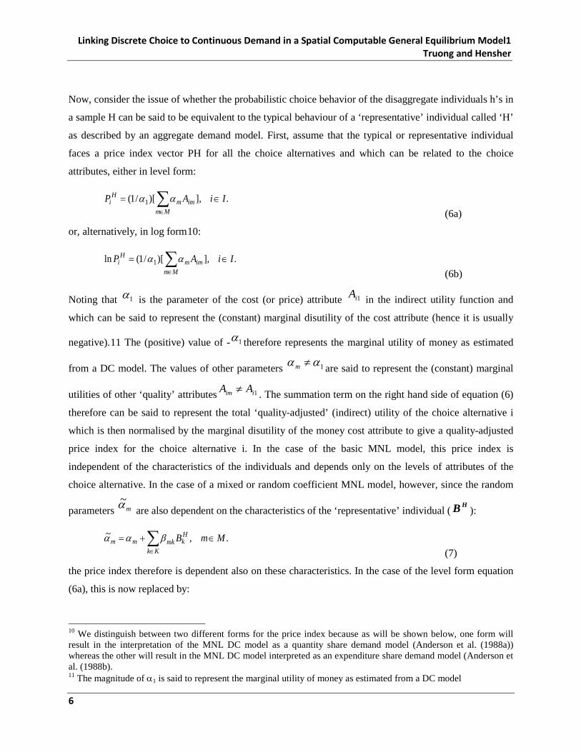
Now, consider the issue of whether the probabilistic choice behavior of the disaggregate individuals h’s in

a sample H can be said to be equivalent to the typical behaviour of a ‘representative’ individual called ‘H’

as described by an aggregate demand model. First, assume that the typical or representative individual

faces a price index vector PH for all the choice alternatives and which can be related to the choice

attributes, either in level form:

.],)[/1( 1 IiAPMm

immH

i ∈= ∑∈

αα (6a)

or, alternatively, in log form10:

.],)[/1(ln 1 IiAPMm

immH

i ∈= ∑∈

αα (6b)

Noting that 1α is the parameter of the cost (or price) attribute 1iA in the indirect utility function and

which can be said to represent the (constant) marginal disutility of the cost attribute (hence it is usually

negative).11 The (positive) value of - 1α therefore represents the marginal utility of money as estimated

from a DC model. The values of other parameters 1αα ≠m are said to represent the (constant) marginal

utilities of other ‘quality’ attributes 1iim AA ≠ . The summation term on the right hand side of equation (6)

therefore can be said to represent the total ‘quality-adjusted’ (indirect) utility of the choice alternative i

which is then normalised by the marginal disutility of the money cost attribute to give a quality-adjusted

price index for the choice alternative i. In the case of the basic MNL model, this price index is

independent of the characteristics of the individuals and depends only on the levels of attributes of the

choice alternative. In the case of a mixed or random coefficient MNL model, however, since the random

parameters mα~ are also dependent on the characteristics of the ‘representative’ individual (HB ):

.,~ MmBKk

Hkmkmm ∈+= ∑

∈

βαα (7)

the price index therefore is dependent also on these characteristics. In the case of the level form equation

(6a), this is now replaced by:

10 We distinguish between two different forms for the price index because as will be shown below, one form will result in the interpretation of the MNL DC model as a quantity share demand model (Anderson et al. (1988a)) whereas the other will result in the MNL DC model interpreted as an expenditure share demand model (Anderson et al. (1988b). 11 The magnitude of α1 is said to represent the marginal utility of money as estimated from a DC model

6


.],~)[~/1( 1 IiAP

Mmimm

Hi ∈= ∑

∈

αα (8a)

Or, alternatively, for the case of equation (6b), this is now replaced by:

.,]~)[~/1(ln 1 IiAPMm

immH

i ∈= ∑∈

αα (8b)

The indirect utility function for each choice alternative can now be expressed in terms of the price index

as follows:

.,1 IiPV Hi

HHi ∈= α (9a)

for the case of the linear price index function (8a); or alternatively

.,)()exp(ln 11 IiPVPV

HHi

Hi

Hi

HHi ∈=⇒= αα (9b)

for the case of the log-price index function (8b).

2.2 MNL DC model as a conditional quantity share demand model

Given the definition of the price index and the indirect utility function for each choice alternative i as

shown by equation (9), the next step is to define the indirect utility function for all choice activities as a

whole. Following from the analysis of Gorman (1961), this (aggregate) indirect utility function for the

‘representative individual will be consistent with the (disaggregate) indirect utilities of all the ‘random’

individuals in the MNL DC model if it is of the Gorman polar form as shown in equation (1), i.e.:

)()(),( H

HHHHHH

gfYYVP

PP −= (10)

where HP is the aggregate price index vector for all choice alternatives as seen by the representative

individual, and HY is the representative individual’s income level. An important issue is the form which

the functions fH(.) and g(.) can take.

Following from Hausman Leonard and McFadden (1995), define g(.) as a ‘logsum’ function as follows12

∑∈

=Ii

iPg )exp(ln1)( γγ

P (11)

Also, using the linear disaggregate price index functions as defined by equation (8a) or (9a), i.e.

ii VP )/1( 1α= , and assuming that = 1α , we have:

12 Henceforth, the superscript ‘H’ will be omitted for simplicity if it is clear that reference is to the ‘representative’ individual rather than to the disaggregate (random) individuals.

7


i

Iii

i

Iii

i

ii Prob

VV

PP

Pgg ===∂

∂=

∑∑∈∈

)exp()exp(

)exp()exp()()(

γγPP (12)

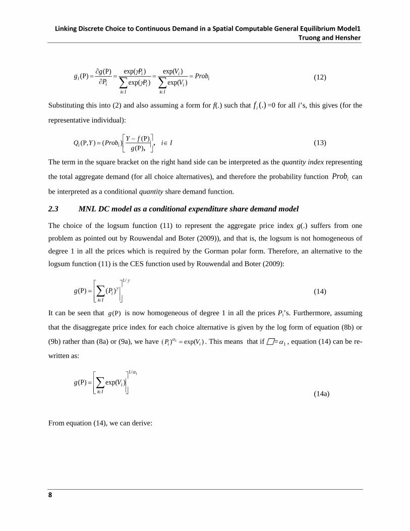
Substituting this into (2) and also assuming a form for f(.) such that (.)if =0 for all i’s, this gives (for the

representative individual):

Iig

fYProbYQ ii ∈

−= ,

,)()()(),(

PPP (13)

The term in the square bracket on the right hand side can be interpreted as the quantity index representing

the total aggregate demand (for all choice alternatives), and therefore the probability function iProb can

be interpreted as a conditional quantity share demand function.

2.3 MNL DC model as a conditional expenditure share demand model

The choice of the logsum function (11) to represent the aggregate price index g(.) suffers from one

problem as pointed out by Rouwendal and Boter (2009)), and that is, the logsum is not homogeneous of

degree 1 in all the prices which is required by the Gorman polar form. Therefore, an alternative to the

logsum function (11) is the CES function used by Rouwendal and Boter (2009):

γγ

/1

)()(

= ∑

∈IiiPg P (14)

It can be seen that )(Pg is now homogeneous of degree 1 in all the prices Pi’s. Furthermore, assuming

that the disaggregate price index for each choice alternative is given by the log form of equation (8b) or

(9b) rather than (8a) or (9a), we have )exp() 1ii VP =( α . This means that if = 1α , equation (14) can be re-

written as:

1/1

)exp()(α

= ∑

∈IiiVg P

(14a)

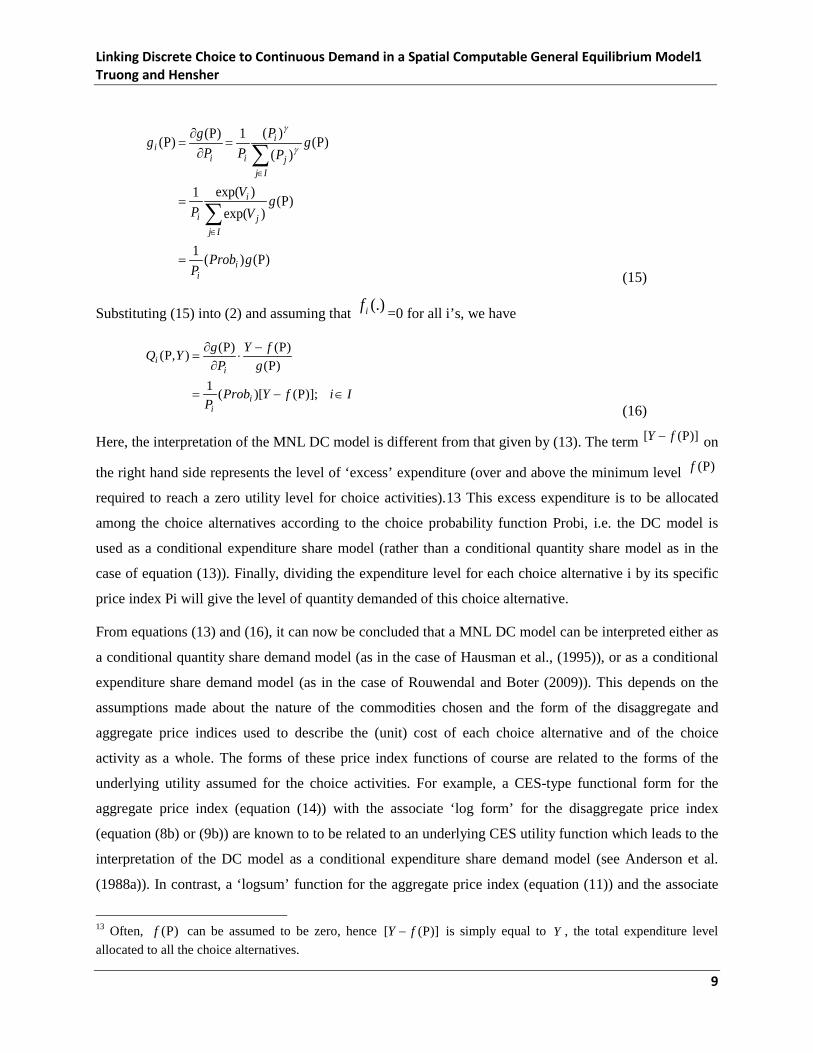
From equation (14), we can derive:

8


)()(1

)()exp(

)exp(1

)()(

)(1)()(

P

P

PPP

gProbP

gV

VP

gP

PPP

gg

ii

Ijj

i

i

Ijj

i

iii

=

=

=∂

∂=

∑

∑

∈

∈

γ

γ

(15)

Substituting (15) into (2) and assuming that (.)if =0 for all i’s, we have

IifYProbP

gfY

PgYQ

ii

ii

∈−=

−⋅

∂∂

=

)];()[(1)(

)()(),(

P

PPPP

(16)

Here, the interpretation of the MNL DC model is different from that given by (13). The term )]([ PfY − on

the right hand side represents the level of ‘excess’ expenditure (over and above the minimum level )(Pf

required to reach a zero utility level for choice activities).13 This excess expenditure is to be allocated

among the choice alternatives according to the choice probability function Probi, i.e. the DC model is

used as a conditional expenditure share model (rather than a conditional quantity share model as in the

case of equation (13)). Finally, dividing the expenditure level for each choice alternative i by its specific

price index Pi will give the level of quantity demanded of this choice alternative.

From equations (13) and (16), it can now be concluded that a MNL DC model can be interpreted either as

a conditional quantity share demand model (as in the case of Hausman et al., (1995)), or as a conditional

expenditure share demand model (as in the case of Rouwendal and Boter (2009)). This depends on the

assumptions made about the nature of the commodities chosen and the form of the disaggregate and

aggregate price indices used to describe the (unit) cost of each choice alternative and of the choice

activity as a whole. The forms of these price index functions of course are related to the forms of the

underlying utility assumed for the choice activities. For example, a CES-type functional form for the

aggregate price index (equation (14)) with the associate ‘log form’ for the disaggregate price index

(equation (8b) or (9b)) are known to to be related to an underlying CES utility function which leads to the

interpretation of the DC model as a conditional expenditure share demand model (see Anderson et al.

(1988a)). In contrast, a ‘logsum’ function for the aggregate price index (equation (11)) and the associate

13 Often, )(Pf can be assumed to be zero, hence )]([ PfY − is simply equal to Y , the total expenditure level allocated to all the choice alternatives.

9


‘linear form’ of the disaggregate price for each choice alternative (equation (8a) or (9a)) can be said to

represent an underlying entropy-type utility function and resulting in the interpretation of the DC model

as a conditional expenditure share demand model (see Anderson et al. (1988b)). Although both of these

types of conditional demand DC models can be used to link to an (unconditional) CD model, it is now

clear that only the CES form and the expenditure share DC model is seen to be consistent with a Gorman

polar utility form approach.14 In the case of the entropy-type utility and logsum aggregate price function,

although the aggregation of all quantity shares may not lead to a consistent aggregation of the

expenditures (and prices), the link between DC and CD model is conducted via an aggregate quantity

index rather than price index, and the latter (relative prices) are used only to distribute the total quantity to

the various alternative choices. The absolute level of the prices may need to be ‘calibrated’ but this is to

be expected because the indirect utility/cost function in a DC model is normally specified only up to an

arbitrary origin.15

3. Linking DC models to CD models in a general equilibrium

framework

As can be seen from the previous section, one way of linking a DC to a CD model is to assume a two-

stage decision process, with the DC decisions representing the ‘lower stages’ which are concerned

primarily with the choices or substitution between varieties of a particular product (such as modes of

travel, types of cars, modes of dwellings, etc.). These lower-stage decisions are then linked to an ‘upper

stage’ which is concerned primarily with the choices or substitution between aggregate groups of

commodities (such as between travel and housing, energy and food, work and recreation, etc.) and which

are subject to a total expenditure constraint. Crucial in the link between lower stage DC models and upper

stage CD models is the formation of the aggregate and disaggregate price/quantity indices which

represent the various choice commodities in the lower and upper stages. These price/quantity indices must

be consistent with each other at all stages. This would not be a problem if both the lower and upper stages

are described in terms of the same theoretical framework but in this case, because there is a mixture of the

random utility structure of a DC model and the deterministic utility structure of a CD model, these

different structures need to be reconciled so as to ensure consistency in aggregation.

14 This result is of no surprise because only the use of a DC model as a conditional expenditure share model that can lead to the obvious result that the aggregation of all individual expenditures of all different choices will always be equal to the total expenditure. The aggregation of quantity shares into an aggregate quantity does not lead to a consistent aggregation of expenditure shares because of the price element. 15 This is because replacing the value of Vi by Vi + C where C is any constant will not change the choice probabilities in the discrete choice model but this will change the value of the price index (logsum) by a constant.

10


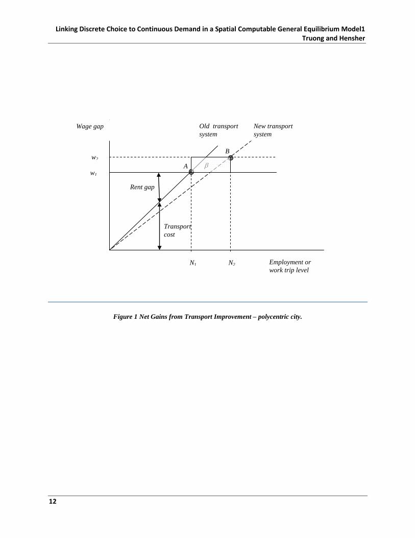
Consider the following example. Assume that there is an improvement in the transport system such that

the (generalised)16 costs of travel along certain routes are reduced. In an economy where the cost of

certain activity (“work”) by an individual consists mainly of travel and housing costs, a reduction in

transport cost can be passed on to housing expenditure (in the form of higher rent due to increasing

demand for housing in a particular area - see, for example, Figure 1, adapted from Venables (2007)).17 In

general, however, such an improvement can also result in a higher level of other activities including

transport itself. To consider this issue, an ‘upper-stage’ demand system may need to be considered where

the income effect of the transport improvement (reduction in transport costs is considered as an increase

in real income for the workers) as well as the substitution effect between transport and all other activities

must be considered (now that the relative price between transport and other commodity prices have

changed). The net result of the income and substitution effects would tell us whether an improvement in

the transport system would result in more (or less) travel and/or other activities. This ultimately would

depend on the structure of the transport system and the pattern of land uses (housing, employment, and

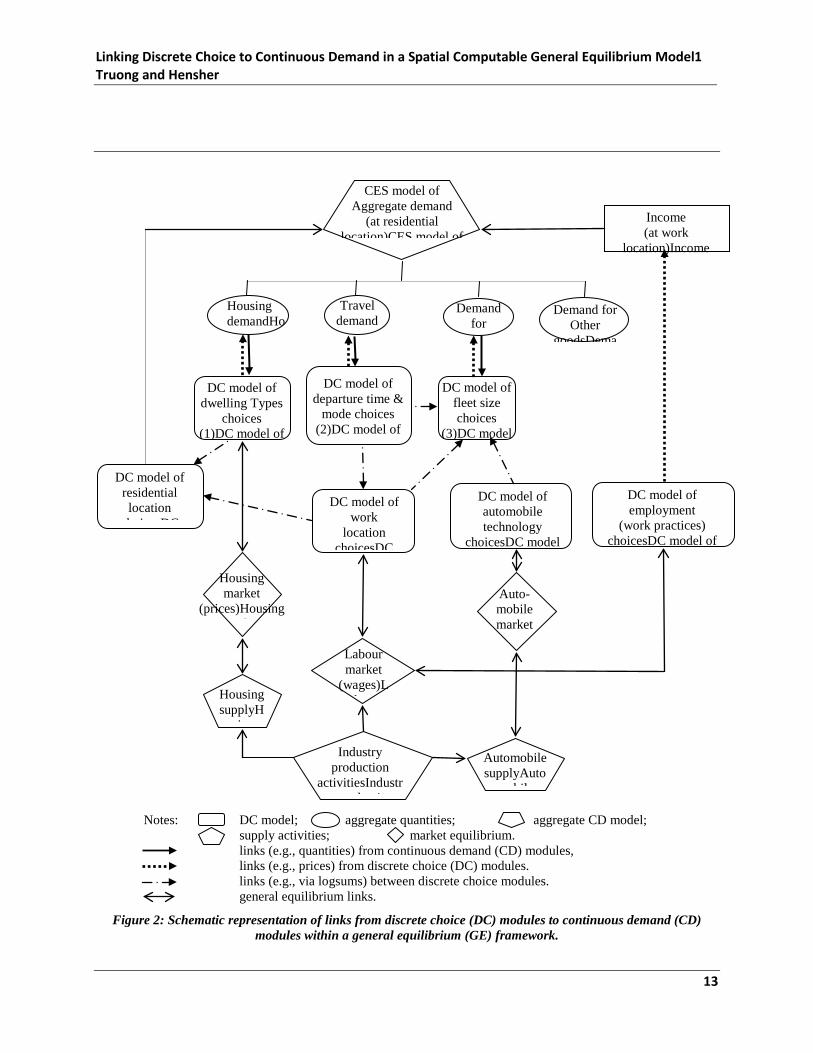
other activities) in a particular city. Therefore, an integrated model of DC and CD module linkages

(Figure 2) must be considered and put in the context of a spatial general equilibrium (SGEM) model of

the city where all the distributions of transport, housing and other economic activities of the city are taken

into account.

16 The generalized costs of travel may include non-monetary costs such as travel time ‘costs’, the (hedonic) ‘costs’ comfort or convenience associated with a particular travel mode, etc. In a DC model of mode choice , the generalized cost of a particular mode can be measured by the value of the indirect utility of the mode divided by the marginal utility of the money cost, i.e. by the (generalized) price index of a mode such as described by equations (8)-(9). 17 Venables (2007) considered only a monocentric city. Here it is adapted to consider a polycentric city where the ‘center of employment’ is a particular zone considered in relation to all other zones. The wage gap, rent gap and commuting costs therefore are measured in terms of the average between the zone and all other employment centers.

11


Figure 1 Net Gains from Transport Improvement – polycentric city.

Transport cost

Rent gap

β

B

N1 N2

w1

w2

New transport system

A

Old transport system

Wage gap

Employment or work trip level

12


Notes: DC model; aggregate quantities; aggregate CD model;

supply activities; market equilibrium. links (e.g., quantities) from continuous demand (CD) modules, links (e.g., prices) from discrete choice (DC) modules. links (e.g., via logsums) between discrete choice modules. general equilibrium links.

Figure 2: Schematic representation of links from discrete choice (DC) modules to continuous demand (CD) modules within a general equilibrium (GE) framework.

DC model of dwelling Types

choices (1)DC model of

DC model of residential location h i DC

DC model of work

location choicesDC

DC model of departure time &

mode choices (2)DC model of

DC model of employment

(work practices) choicesDC model of

DC model of fleet size choices

(3)DC model

CES model of Aggregate demand

(at residential location)CES model of

Housing demandHo

Travel demand

Demand for

Income (at work

location)Income

DC model of automobile technology

choicesDC model

Demand for Other

goodsDema

Industry production

activitiesIndustr d ti

Housing market

(prices)Housing k

Labour market

(wages)Lb

Housing supplyH

i

Automobile supplyAuto

bil

Auto- mobile market

( i )A

13


To simplify the analysis, assume that an upper CD demand module consists only of a decision between

travel and housing expenditures.18 Let )1(P and )2(P be the aggregate19 price indices of ‘travel’ and

‘housing’ activities respectively which are estimated from the DC models as explained in the previous

sections, and let M be the total budget allocated to travel and housing activities. The aggregate demand

for travel and housing activities is then given by the following optimisation problem:

[ ]MQPQP

QQQQUU≤+

+==)2()2()1()1(

/1)2(2

)1(1

)2()1(

s.t.

)()(),( Maximise ρρρ δδ (17)

where )1(Q and )2(Q are the aggregate levels of demand for travel and housing activities respectively, δ1

and δ2 are the distribution parameters of the CES utility function, and = 1/(1) is a parameter

representing the elasticity of substitution between these aggregate activities. The solution for the above

maximisation problem depends on the form of the utility function U(.), and in the case when this function

is assumed to be of a CES form20 the solution will be given as follows:

[ ] }.2,1{;)()()/( 1)()()()( =+=− nQQPMQ n

nn

nn

nn ρρσ δδδ (18)

To simplify the expression, a ‘percentage change’ form can be used in place of the absolute level form of

equation (19). Using a lower case letter to denote the percentage change (or differential log) form of an

upper case variable, we have:

}2,1{];[

][)(

][)(

])1([

)(

}2,1{

)()(

}2,1{

)(

}2,1{

)()(

}2,1{

)(

}2,1{

)()()(

=−−=

−−=

−−−=

−−−=

∑∑

∑∑

∑

==

==

=

nppq

pSpqS

pSppSm

pSpmq

n

k

kk

n

k

kk

k

kk

n

k

kk

k

kk

nn

σ

σ

σ

σσ

(19)

where:

18 The inclusion of other goods into the CD system will change the details but not the broad conclusions of the analysis. 19 A variable without a subscript is used to refer to the aggregate level (i.e. summarized over all lower-stage choices). This is to be distinguished from the disaggregate variable which has a subscript to indicate the specific choice alternative in each lower-stage decision. 20 Other forms can also be used without affecting the main conclusions of the analysis.

14


}2,1{;ln;ln )()()()( === nQdqPdp nnnn (20)

}.2,1{;)()(

)()(

}2,1{

1)(

1)()()(

===

∑=

−

−

nP

PMQPS

k

kk

nn

nn

nσσ

σσ

δ

δ (21)

∑=

=}2,1{

)(

n

nn pSp (22)

∑=

=}2,1{

)(

n

nnqSq (23)

pqpqSMdm n

n

nn +=+== ∑

=

)(ln )(

}2,1{

)( (24)

Given the aggregate demand functions (18) (or (19)), the distribution of the aggregate demand into

various travel and housing choice alternatives can then be described by the lower-stage DC models.

3.1 Quantity share DC model linked to a CD model

Assume that the DC module of travel mode choice is interpreted as a demand quantity share (rather than

expenditure share) model which describes the distribution of a fixed total quantity of travel demand (total

number of work trips) from a particular residential location to a particular work location (Origin-

Destination pair) by various modes. The reason why a travel mode choice module is regarded as a

demand quantity share rather than expenditure share model can be explained as follows. Firstly, travel to

work is an intermediate rather than final (household production) activity and therefore so long as the same

destination is reached, it is immaterial which particular mode has been used. The ‘trips’ by different

modes therefore can be regarded as though perfect substitutes, and their quantities simply be added up.

The differences in qualities of travel can be reflected in the ‘quality-adjusted price indices’ of travel, and

because of the ‘random’ components in these prices (derived from a random utility structure) the

aggregation of individual price indices into an aggregate price must be carried out in a consistent fashion,

and this has been discussed in the previous sections. Because travel mode choice decision is regarded as a

quantity-share demand decision, the appropriate price index structures for travel mode choice decisions

are given by equations (9a) and (11) and therefore we can write:

∑

∑

∈

∈

=

=

)1(

)1(

)exp(ln1

)exp(ln1

)1()1(

1

)1()1()1(

)1(

Iii

Iii

V

PP

α

γγ

(25)

15


where (1)= )1(1α is the coefficient of the money cost attribute in the discrete travel mode choice model,

)1(iV is the indirect utility of choice alternative i in the travel mode choice set )1(I . Taking the absolute

differential21 of this aggregate price index, we have:

)1()1(

1

)1()1(

1

)1()1()1(

)1(

1

)exp(ln1

)exp(ln1

)1(

)1(

Vd

Vd

PddP

Iii

Iii

α

α

γγ

=

=

=

∑

∑

∈

∈

(26)

where

)1()1(

)1()1(

)1(

)1()1(

)1(

)1(

)1(

)1(

)exp(

)exp

)exp(ln

jIj

j

jIj k

Ik

j

Iii

dVProb

dVV

V

VdVd

∑

∑ ∑

∑

∈

∈∈

∈

=

=

=

(27)

Since the discrete travel mode choice model is used as a conditional quantity share demand model, this

implies:

])[()( )1()1()1()1()1( QProbYQ ii ≡,P (28)

where )1(iQ stands for the level of demand (number of choices) for travel mode choice alternative i, )1(Q

is the aggregate level of demand for all mode choices which is assumed to be given exogeneously of a DC

model but which can be estimated from an upper-stage CD module using equation (18) or (19), and

)( )(niProb is the choice probability from the lower-stage DC model. Taking the differential log of both

sides of equation (28) and using a lower case letter to denote these differential log (or percentage change)

terms, we have:

)ln( )1()1()1(ii Probdqq += (29)

21 Note that equation (20) requires information on the percentage change (or differential log) of the aggregate price indices, therefore, to get this value the absolute differential of equation (26) needs to be divided by the initial value of the aggregate price index which is given by equation (25). As noted from the previous sections, the use of a logsum formula to define the aggregate price index for a DC model requires that its initial value be ‘calibrated’ so that it is consistent with the initial values of the expenditure level and quantity of all the choices.

16


where:

)1()1(

)1()1()1( )exp(ln)ln(exp()ln()1(

VddV

VdVdProbd

i

jTj

ii

−=

−= ∑∈ (30)

The first term on the right hand side of equation (29) stands for the total quantity effect as estimated from

the upper-stage CD model (20), and the last term on the right hand side of equation (29 measures the

quantity substitution effect (i.e. the percentage change in the quantity share of alternative i) which can be

estimated from the lower-stage DC model using equation (30).

3.2 Expenditure share DC model linked to a CD model

Now consider the case of the aggregate housing location/type choice decision which is also estimated

from the upper-stage CD model jointly with the aggregate travel demand decision (as seen from equation

(19)) but linked to a lower-stage DC model which is interpreted as a housing expenditure share rather

than quantity share model. The reason for the interpretation of housing location/type choice decision as a

demand expenditure share rather than a demand quantity share decision is given as follows. Firstly,

housing quantities in different locations and of different types cannot really be regarded as though

‘perfect substitutes’. They are essentially different commodities with significantly different attributes and

levels of expenditure. Therefore, their substitution can only be handled via a consideration of the relative

price structures and income effects rather than as a matter of quantity substitution.In this case, The

aggregate price index for an expenditure share CD module is therefore by equation (9b) and (14) (CES

function rather than logsum function):

)2(1

)2(

)2(

)2(

)2(

/1)2(

/1)2()2(

)exp(

)(

α

γ

γ

=

=

∑

∑

∈

∈

Iii

Iii

V

PP

(31)

where (2)= )2(1α is the coefficient of the money cost attribute in the discrete housing type/location choice,

and )2(iV is the indirect utility of the housing type/location choice alternative i in this DC model. Taking

the differential log of both sides of equation (31) gives:

17


)2()2(

1

)2()2(

1

)2()2()2(

)2(

1

)exp(ln1

)exp(ln1ln

)2(

)2(

Vd

Vd

PdPd

Iii

Iii

α

α

γγ

=

=

=

∑

∑

∈

∈

(32)

This is essentially the same as equation (26) except that the left hand side stands for the percentage

change (or log change) in the price index rather than an absolute change. This is explained as follows.

The right hand sides (of both equations (26) and (31)) represent the absolute change in the logsum

(normalised by the marginal utility of money). For a DC model, the logsum is determined only up to an

arbitrary origin, but its absolute change is fully determined and therefore can be used to indicate the

absolute change in total indirect utility associated with all choices. When this change in indirect utility is

normalised by the marginal utility of money it can be used to represent the change in cost or expenditure

level associated with the choice decisions. Now, for a quantity share DC model, the total quantity of all

choices is assumed to be fixed or given exogeneously of the model and therefore can be normalised to 1

initially (for a DC model). This means the absolute change in the cost or expenditure level (right hand

side of equation (26)) can also be used to indicate the absolute change in price index (left hand side of

equation (26)). For an expenditure share DC model, however, the total level of expenditure (rather than

total quantity) is assumed to be fixed or given exogeneously of the DC model therefore the initial total

expenditure or (aggregate price level) can be normalised to 1 initially.22The absolute change in

expenditure or aggregate price level (right hand side of equation (32)) now represents also the percentage

(or log) change.23

Given that the DC model is used as an expenditure share rather than a quantity share demand model, the

absolute demand quantity for each housing location/type choice alternative i is then given by:

])[(1)( )2()2()2()2(

)2()2()2( QPProbP

YQ ii

i ≡,P (33)

where )2(iP is the disaggregate price index for housing choice alternative i (as defined by equation (9b)),

)2()2( QP is the total expenditure level for housing activities, and )( )2(iProb is the choice probability for

22 This normalisation requires the calibration of the initial indirect utilities in equation (31)such that the aggregate price level is equal to 1 initially. This means the logsum in equation (32) is equal to zero initially. 23 In fact, from equation (9b), the indirect utility function of an expenditure share DC model is specified as the log-price rather than linear price of the choice alternative, hence the absolute change in the ‘expected’ indirect utility (i.e

)2(Vd

in equation 32) must also be said to represent the log change in aggregate price.

18


the housing choice alternative i as determined by the lower-stage DC model. Taking the differential log of

both sides of equation (33) gives:

)ln(][ )2()2()2()2()2(iii Probdppqq +−−= (34)

Compared to the demand for travel mode choice activities as represented by equation (30) of the previous

section, the demand for housing choice activities in equation (35) is slightly different. Firstly, apart from

the first term which represents the total quantity effect as estimated from the upper-stage CD model of

equation (20) - which remains the same in both cases, the very last term on the right hand side of equation

(34) now represents the percentage change in expenditure sharerather than quantity share as in the case of

equation (30). Since expenditure share involves a relative price component in addition to the quantity

components, the middle terms within the square brackets on the right hand side of equation (34) are used

to offset this relative price effects. To estimate this relative price effect, firstly, taking the differential log

of the disaggregate price index in equation (9b) will give:

)2()2()2()2( )/1(ln iiii dVPdp α== (35)

Next, from equation (32) this can also be written as :

)2()2(1

)2( )/1( Vdp α= (36)

Therefore, the relative price effect is given as:

])[/1()/ln(][ )2()2()2()2()2()2()2(iiiiiii VddVPPdpp −==− α (37)

Substituting this into equation (34) gives:

])[11( )2()2()2(

1

)2()2( VddVqq ii −−+=α

(38)

Comparing equation (38) to equation (30), the difference is in the extra term representing the relative

price effect.

19


4. An Illustrative experiment

To illustrate the applicability of the approach described in the previous section for linking DC to CD

models within a CGE framework, we consider a simple experiment.24 In this experiment, we investigate

the impacts of a transport infrastructure investment project in the Sydney Metropolitan Area (SMA) on

transport users and on the local economy. The impacts on transport users are traditionally estimated using

a collection of DC modules25 set up within a ‘bottom-up’ partial equilibrium (PE) model such as

TRESIS.26 The use of these DC modules requires an implicit assumption that all other activities ‘outside’

of the DC decisions (for example, total levels of travel and housing demand) are given exogenously of the

DC modules. However, these activity levels can in practice be affected by, as well as affecting, the

decisions within the DC modules, therefore, to explore the important linkages between the DC decisions

and CD decisions, a PE model such as TRESIS needs to be linked to some ‘upper-stage’ CD modules.

For example, to estimate the extent of the substitution or interaction between travel and housing activities,

the results from the discrete mode choice and dwelling-type choice modules are used as inputs into the

CD module which represents the interaction (at the aggregate level) between travel and housing activities

as explained in the previous sections. Both the DC and CD modules are then immersed in a spatial

computable general equilibrium model (SCGE) which represents the local economy to determine how

much of the improvement in the transport system (in the form of reduced transport costs for certain links

in the transport system) can be translated into (i) improved labour productivity at work locations (due to

the so-called ‘agglomeration effects’) which can lead to increased wage levels for certain industry sectors

in certain locations, and (ii) increase in rents for certain locations due to improved transport links to these

locations (this can be referred to as the ‘Venables effect’ – see Figure 1). Improved labour productivity

due to agglomeration effects in some locations, however, may also lead to ‘disagglomeration’ effects

elsewhere due to spatial competition between locations. Therefore, the ‘general equilibrium’ effects of a

transport improvement may include both winners and losers in terms of changes in wage and rent levels

in various locations.

24 For more details on this experiment, see Truong and Hensher (2012) and Hensher et al. (2012). 25 To distinguish between the larger system of interconnected models such as TRESIS or a CGE model and the smaller individual DC (or CD) models within this system, we use the term ‘module’ to refer to the latter and reserve the term ‘model’ to refer only to the larger complete system. Thus, a ‘model’ can consist of several different ‘modules’ within it. 26 See Hensher (2002); Hensher and Ton (2002).

20


4.1 Discrete-choice decisions without linkage to continuous demand decisions

Tables 1 shows the effect of the transport improvement in the rail link between zone 1 (Inner Sydney) and

zone 10 (Blacktown Baulkham Hills) on the generalised cost of travel by train between different zones

(see Figure A1 for a description of the zones). Table 2 shows the percentage change in the probability of a

worker choosing train as the mode of transport for the work trip between these zones. Quite clearly, with

the reduction in travel time between zone 10 and other zones, the probability of choosing train as the

preferred mode of transport to and from zone 10 will increase, while the probability of choosing other

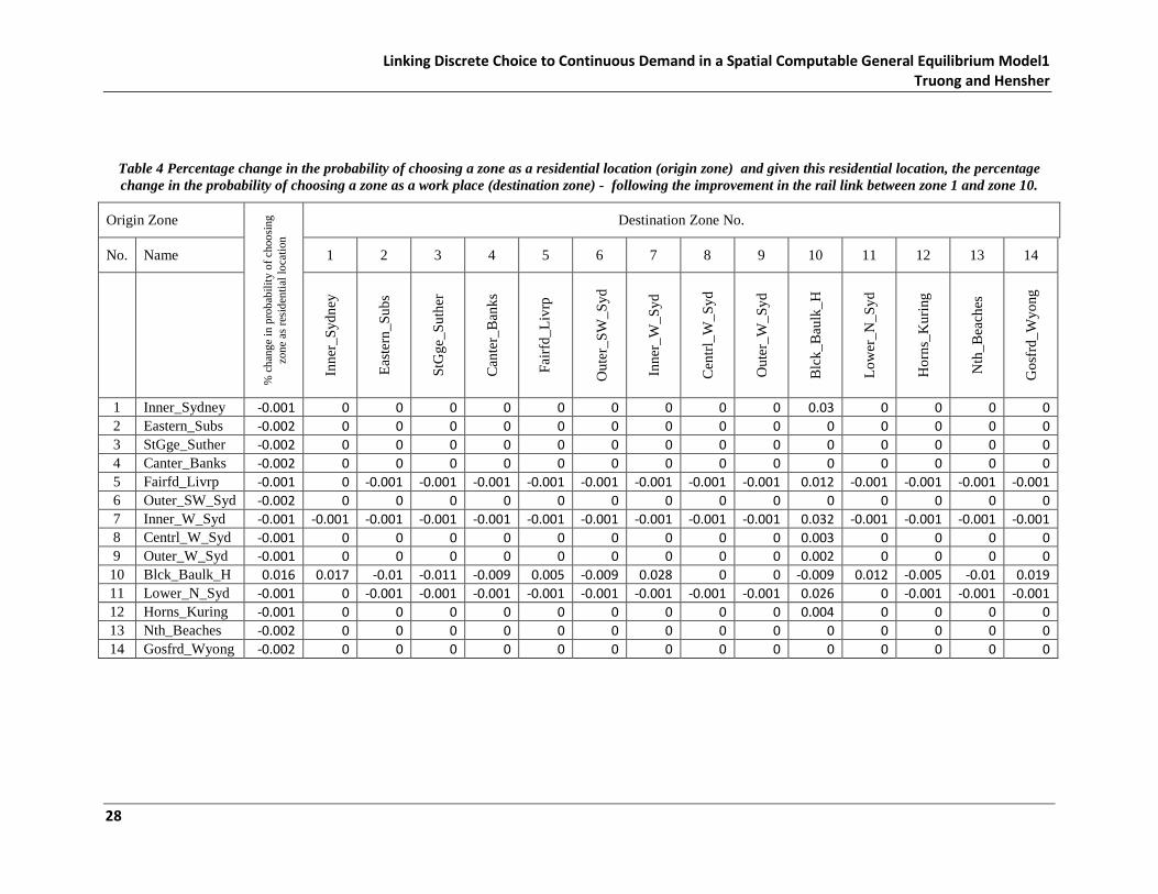
modes will decrease (Table 3). Residential and work location choices are also affected by the transport

improvement, and this is shown in Table 4. Here it is seen that zone 10 can become a preferred place of

residence even though workers living in zone 10 may now prefer to work in locations other than zone 10

(for example, in zone 1 (Inner_Sydney), 5 (Fairfield_Liverpool), 7 (Inner_West) and 11

(Lower_North_Sydney). The magnitude of these changes, however, are quite small, implying that the

direct impacts of transport improvement on land uses are small.

4.2 Discrete-choice decisions with linkage to continuous demand decisions in a general equilibrium setting

Assuming that transport and land use decisions by the workers can be translated into housing and

employment activities in the local economy,27 we can now look at the potential impacts of changes in the

transport network on the housing and labour market. Firstly, with respect to the housing market,

residential location choices and dwelling type choices will affect dwelling demand, which in turn will

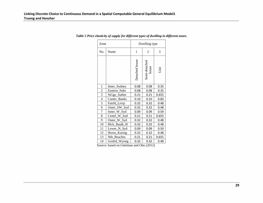
induce changes in dwelling supply and dwelling prices. Dwelling supply is here assumed to be

responding to changes in dwelling prices. The price elasticity of supply of dwellings for various locations

in the Sydney metropolitan area is taken from a study by Gitelman and Otto (2012) (see Table 5). Given

the potential interactions between supply and demand in various zones, equilibrium results are shown in

Table 6 (when DC results are not linked to upper-stage CD decisions) and Table 7 (when DC results are

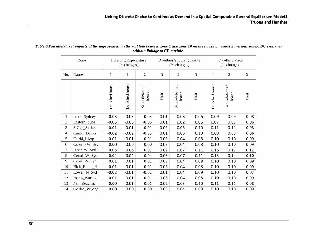
not linked to upper-stage CD decisions). Here it is seen that for a relatively small infrastructure project

like the NWRL rail link improvement, the direct impacts of the transport improvement on housing

activities would be small (Table 6). By ‘direct’ impacts, this is meant to be attributed only to changes in

residential location and work location decisions as estimated from DC modules without linkage to an

upper-stage continuous demand module which focuses attention on the aggregate trade-off between

housing and travel decisions as well as on the ‘income’ effect of reduced transport costs on travel and

27 This requires changes on the supply side (i.e. housing supply and employment opportunities) as well as changes on the demand side as induced by changes in household residential and work location choices.

21


housing activities (the ‘Venables’ effect). When these indirect impacts are also taken into account, the

total impacts of transport improvement on housing activities can be seen to be more substantial (see Table

7). Here, the ‘income’ effect of transport improvement on housing activities are seen to be most

significant for zone 10 (as is expected), but other zones also benefit significantly. Table 8 shows the

indirect effects as captured by the upper-stage CD module. The indirect effects would consist not only of

the aggregate income effects but also aggregate substitution effects between transport and housing.

Following an improvement in the transport system, the aggregate price of transport would have been

reduced relative to the price of housing which means a substitution away from housing expenditure

towards ‘cheaper’ transport (i.e. workers move places of residence away from the work place towards

locations which have cheaper rents (imputed or actual) but requiring greater travel. In a general

equilibrium framework, however, this substitution effect would be counter balanced by an opposite (real)

income effect where the reduced cost of transport cost would imply an increase in real income and

therefore increased level of expenditure on both housing and travel activities. The net impacts of these

two opposite effects are shown in Table 8 for the case of housing activities.

For transport activities, the improvement in the rail link between zones 1 and 10 would imply not only a

direct substitution effect between different modes of transport as captured by DC module of mode choice

(see Tables 2-3) but also between different zones (as places of residence and/or work places – see Table

4). Therefore, the net impacts of these direct effects on train travel could be negative for some zones (for

example, zones 4 and 5 - see Table 9) even though they are mostly positive for all other zones. In addition

to the direct effects, however, there are also indirect effects from aggregate income and substitution

effects between travel and housing (i.e. location or land use) activities. Therefore, these indirect effects

may counteract the direct effects to such an extent that it can reverse the original direction of the direct

impacts. This is seen for the cases of zones 6 and 8 (Outer_SW_Syd and Centrl_W_Syd), see Table 10.

The reduction (rather than increase) in train travel to these locations from all zones (except from zone 10)

is seen to arise primarily from a change in place of employment, from zone 6, 8 (and also to some extent,

zone 4) to all other zones especially zones 5 (Fairfield_Liverpool), 7 (Inner_West_Sydney) and of course

also zone 10 (see Table 12)

.

22


5. Conclusion

In this paper we have presented a methodology for linking a disaggregate discrete choice (DC) model to

an aggregate continuous demand (CD) model and integrate both types of models into the framework of a

simple28 spatial computable general equilibrium (SCGE) which represents the local economy of the

Sydney Metropolitan Area (SMA). In this simple model, only a limited number of economic activities are

considered: residential location and dwelling type choices, work place location choices, and mode choice

activities. These disaggregate choice decisions by individual workers are modelled by discrete-choice

(DC) modules contained in a well-known ‘bottom-up’ transport-land use partial equilibrium model called

TRESIS (Hensher and Ton (2002)). The paper presents a methodology for linking these DC modules to a

conventional aggregate continuous demand (CD) module which handles the issue of transport – housing

expenditure substitution but taking into account the complementaty aspects of these decisions in the

context of a spatial general equilibrium model. The methodology is new because up to now, the two types

of DC and CD models are often used for different applications with different contexts, relying on

different theoretical assumptions and to explain different types of behaviour: individual discrete choices

versus continuous aggregate (or ‘representative’) demand behaviour of a consumer. DC models are used

in a ‘bottom-up’ context because it contains great details on individual attributes and technological or

environmental characteristics at a disaggregate level. CD models on the other hand are used in a ‘top-

down’ approach because it can concentrate on ‘economy-wide’ impacts. Linking these bottom-up to top-

down modules is an important challenge not only because of the potential benefits it can bring but also

because of the theoretical and empirical difficulties it must overcome due to the differences between the

two types of models. This paper has shown a methodology for meeting with this challenge and

demonstrated with an empirical example, which shows the potential benefits that can be gained from such

a methodology. More specifically, it shows that measuring the impacts of a transport system improvement

on a local economy (such as the SMA economy) can be difficult because of the potential interactions

between many different types of decisions, not only from the demand side (for example, residential

location and dwelling type choice versus travel activities) but also from the supply side (housing supply

and wage level associated with a particular work location choice). Using only one particular type of

model (e.g. DC models) can concentrate on one type of impacts (e.g. direct impacts of transport

improvement on mode choice or locational choice) but neglecting the indirect impacts (or feedbacks) of

housing and employment activities on these transport decisions themselves. In a modern city with many

‘nodes’ of employment and residential locations, the direction of these impacts can be difficult to trace

28 In this simple model, only work place, residence location and mode choice activities are considered s

23


because of the interplay between the economic and spatial elements, therefore the linkage between DC

and CD modules need to be put in the context of a spatial general equilibrium model (SGEM) to be of

effective use. The paper has shown that this approach is feasible, for a simple (but sufficiently

comprehensive) SGEM such as that for the SMA. The challenge is to extend this methodology to the case

of more complex SGEM, such as that for a state or a nation, and this is left for future contributions

24


Table 1 Percentage change in the generalised cost of TRAIN travel between Origin-Destination zones following an improvement in the RAIL link between zone 1 and zone 10.

Origin Zone Destination Zone No.

No. Name 1 2 3 4 5 6 7 8 9 10 11 12 13 14

Inne

r_Sy

dney

East

ern_

Subs

StG

ge_S

uthe

r

Can

ter_

Ban

ks

Fairf

d_Li

vrp

Out

er_S

W_S

yd

Inne

r_W

_Syd

Cen

trl_W

_Syd

Out

er_W

_Syd

Blc

k_B

aulk

_H

Low

er_N

_Syd

Hor

ns_K

urin

g

Nth

_Bea

ches

Gos

frd_

Wyo

ng

1 Inner_Sydney 0 0 0 0 0 0 0 0 0 -1.9 0 0 0 0 2 Eastern_Subs 0 0 0 0 0 0 0 0 0 -2.43 0 0 0 0 3 StGge_Suther 0 0 0 0 0 0 0 0 0 -3.76 0 0 0 0 4 Canter_Banks 0 0 0 0 0 0 0 0 0 -0.72 0 0 0 0 5 Fairfd_Livrp 0 0 0 0 0 0 0 0 0 -5.7 0 0 0 0 6 Outer_SW_Syd 0 0 0 0 0 0 0 0 0 -3.59 0 0 0 0 7 Inner_W_Syd 0 0 0 0 0 0 0 0 0 -3.88 0 0 0 0 8 Centrl_W_Syd 0 0 0 0 0 0 0 0 0 -8.87 0 0 0 0 9 Outer_W_Syd 0 0 0 0 0 0 0 0 0 -7.13 0 0 0 0 10 Blck_Baulk_H -2.18 -2.7 -3.94 -0.81 -6.22 -3.75 -4.24 -10.6 -7.81 -0.56 -2.19 -2.4 -18.13 -3.33 11 Lower_N_Syd 0 0 0 0 0 0 0 0 0 -1.96 0 0 0 0 12 Horns_Kuring 0 0 0 0 0 0 0 0 0 -2.11 0 0 0 0 13 Nth_Beaches 0 0 0 0 0 0 0 0 0 -18.13 0 0 0 0 14 Gosfrd_Wyong 0 0 0 0 0 0 0 0 0 -3.08 0 0 0 0

25


Table 2 Percentage change in the probability of choosing TRAIN as the mode of transport between Origin-Destination zones following an improvement in the rail link between zone 1 and zone 10.


No. Name 1 2 3 4 5 6 7 8 9 10 11 12 13 14

In

ner_

Sydn

ey

East

ern_

Subs

StG

ge_S

uthe

r

Can

ter_

Ban

ks

Fairf

d_Li

vrp

Out

er_S

W_S

yd

Inne

r_W

_Syd

Cen

trl_W

_Syd

Out

er_W

_Syd

Blc

k_B

aulk

_H

Low

er_N

_Syd

Hor

ns_K

urin

g

Nth

_Bea

ches

Gos

frd_

Wyo

ng

1 Inner_Sydney 0 0 0 0 0 0 0 0 0 4.79 0 0 0 0 2 Eastern_Subs 0 0 0 0 0 0 0 0 0 14.23 0 0 0 0 3 StGge_Suther 0 0 0 0 0 0 0 0 0 22.12 0 0 0 0 4 Canter_Banks 0 0 0 0 0 0 0 0 0 2.32 0 0 0 0 5 Fairfd_Livrp 0 0 0 0 0 0 0 0 0 20.22 0 0 0 0 6 Outer_SW_Syd 0 0 0 0 0 0 0 0 0 22.12 0 0 0 0 7 Inner_W_Syd 0 0 0 0 0 0 0 0 0 17.05 0 0 0 0 8 Centrl_W_Syd 0 0 0 0 0 0 0 0 0 21.61 0 0 0 0 9 Outer_W_Syd 0 0 0 0 0 0 0 0 0 21.71 0 0 0 0 10 Blck_Baulk_H 4.78 14.23 22.12 2.32 19.91 22.12 16.14 20.6 20.8 1.32 6.34 9.88 22.12 18.48 11 Lower_N_Syd 0 0 0 0 0 0 0 0 0 5.86 0 0 0 0 12 Horns_Kuring 0 0 0 0 0 0 0 0 0 9.9 0 0 0 0 13 Nth_Beaches 0 0 0 0 0 0 0 0 0 22.12 0 0 0 0 14 Gosfrd_Wyong 0 0 0 0 0 0 0 0 0 23.03 0 0 0 0

26


Table 3 Percentage change in the probability of choosing modes OTHER THAN TRAIN as the mode of transport between Origin-Destination zones following an improvement in the rail link between zone 1 and zone 10.


No. Name 1 2 3 4 5 6 7 8 9 10 11 12 13 14

Inne

r_Sy

dney

East

ern_

Subs

StG

ge_S

uthe

r

Can

ter_

Ban

ks

Fairf

d_Li

vrp

Out

er_S

W_S

yd

Inne

r_W

_Syd

Cen

trl_W

_Syd

Out

er_W

_Syd

Blc

k_B

aulk

_H

Low

er_N

_Syd

Hor

ns_K

urin

g

Nth

_Bea

ches

Gos

frd_

Wyo

ng

1 Inner_Sydney 0 0 0 0 0 0 0 0 0 -3.83 0 0 0 0 2 Eastern_Subs 0 0 0 0 0 0 0 0 0 0 0 0 0 0 3 StGge_Suther 0 0 0 0 0 0 0 0 0 0 0 0 0 0 4 Canter_Banks 0 0 0 0 0 0 0 0 0 -0.05 0 0 0 0 5 Fairfd_Livrp 0 0 0 0 0 0 0 0 0 -1.56 0 0 0 0 6 Outer_SW_Syd 0 0 0 0 0 0 0 0 0 0 0 0 0 0 7 Inner_W_Syd 0 0 0 0 0 0 0 0 0 -4.15 0 0 0 0 8 Centrl_W_Syd 0 0 0 0 0 0 0 0 0 -0.42 0 0 0 0 9 Outer_W_Syd 0 0 0 0 0 0 0 0 0 -0.34 0 0 0 0 10 Blck_Baulk_H -3.84 0 0 -0.05 -1.81 0 -4.9 -1.25 -1.08 -0.04 -2.98 -0.53 0 -3.7 11 Lower_N_Syd 0 0 0 0 0 0 0 0 0 -3.42 0 0 0 0 12 Horns_Kuring 0 0 0 0 0 0 0 0 0 -0.51 0 0 0 0 13 Nth_Beaches 0 0 0 0 0 0 0 0 0 0 0 0 0 0 14 Gosfrd_Wyong 0 0 0 0 0 0 0 0 0 0 0 0 0 0

27


Table 4 Percentage change in the probability of choosing a zone as a residential location (origin zone) and given this residential location, the percentage change in the probability of choosing a zone as a work place (destination zone) - following the improvement in the rail link between zone 1 and zone 10.

Origin Zone

% c

hang

e in

pro

babi

lity

of c

hoos

ing

zone

as r

esid

entia

l loc

atio

n Destination Zone No.

No. Name 1 2 3 4 5 6 7 8 9 10 11 12 13 14

Inne

r_Sy

dney

East

ern_

Subs

StG

ge_S

uthe

r

Can

ter_

Ban

ks

Fairf

d_Li

vrp

Out

er_S

W_S

yd

Inne

r_W

_Syd

Cen

trl_W

_Syd

Out

er_W

_Syd

Blc

k_B

aulk

_H

Low

er_N

_Syd

Hor

ns_K

urin

g

Nth

_Bea

ches

Gos

frd_

Wyo

ng

1 Inner_Sydney -0.001 0 0 0 0 0 0 0 0 0 0.03 0 0 0 0 2 Eastern_Subs -0.002 0 0 0 0 0 0 0 0 0 0 0 0 0 0 3 StGge_Suther -0.002 0 0 0 0 0 0 0 0 0 0 0 0 0 0 4 Canter_Banks -0.002 0 0 0 0 0 0 0 0 0 0 0 0 0 0 5 Fairfd_Livrp -0.001 0 -0.001 -0.001 -0.001 -0.001 -0.001 -0.001 -0.001 -0.001 0.012 -0.001 -0.001 -0.001 -0.001 6 Outer_SW_Syd -0.002 0 0 0 0 0 0 0 0 0 0 0 0 0 0 7 Inner_W_Syd -0.001 -0.001 -0.001 -0.001 -0.001 -0.001 -0.001 -0.001 -0.001 -0.001 0.032 -0.001 -0.001 -0.001 -0.001 8 Centrl_W_Syd -0.001 0 0 0 0 0 0 0 0 0 0.003 0 0 0 0 9 Outer_W_Syd -0.001 0 0 0 0 0 0 0 0 0 0.002 0 0 0 0 10 Blck_Baulk_H 0.016 0.017 -0.01 -0.011 -0.009 0.005 -0.009 0.028 0 0 -0.009 0.012 -0.005 -0.01 0.019 11 Lower_N_Syd -0.001 0 -0.001 -0.001 -0.001 -0.001 -0.001 -0.001 -0.001 -0.001 0.026 0 -0.001 -0.001 -0.001 12 Horns_Kuring -0.001 0 0 0 0 0 0 0 0 0 0.004 0 0 0 0 13 Nth_Beaches -0.002 0 0 0 0 0 0 0 0 0 0 0 0 0 0 14 Gosfrd_Wyong -0.002 0 0 0 0 0 0 0 0 0 0 0 0 0 0

28


Table 5 Price elasticity of supply for different types of dwelling in different zones.

Zone Dwelling type

No. Name 1 2 3

Det

ache

d ho

use

Sem

i-det

ache

d ho

use

Uni

t

1 Inner_Sydney 0.08 0.08 0.35 2 Eastern_Subs 0.08 0.08 0.35 3 StGge_Suther 0.21 0.21 0.655 4 Canter_Banks 0.10 0.10 0.83 5 Fairfd_Livrp 0.32 0.32 0.48 6 Outer_SW_Syd 0.32 0.32 0.48 7 Inner_W_Syd 0.09 0.09 0.59 8 Centrl_W_Syd 0.21 0.21 0.655 9 Outer_W_Syd 0.32 0.32 0.48 10 Blck_Baulk_H 0.32 0.32 0.48 11 Lower_N_Syd 0.09 0.09 0.59 12 Horns_Kuring 0.32 0.32 0.48 13 Nth_Beaches 0.21 0.21 0.655 14 Gosfrd_Wyong 0.32 0.32 0.48

Source: based on Gitelman and Otto (2012)

29


Table 6 Potential direct impacts of the improvement in the rail link between zone 1 and zone 10 on the housing market in various zones: DC estimates without linkage to CD module.

Zone Dwelling Expenditure (% changes)

Dwelling Supply Quantity (% changes)

Dwelling Price (% changes)

No. Name 1 1 2 3 2 3 1 2 3

Det

ache

d ho

use

Det

ache

d ho

use

Sem

i-det

ache

d ho

use

Uni

t

Sem

i-det

ache

d ho

use

Uni

t

Det

ache

d ho

use

Sem

i-det

ache

d ho

use

Uni

t

1 Inner_Sydney -0.03 -0.03 -0.03 0.01 0.03 0.06 0.09 0.09 0.08 2 Eastern_Subs -0.05 -0.06 -0.06 0.01 0.02 0.05 0.07 0.07 0.06 3 StGge_Suther 0.01 0.01 0.01 0.02 0.05 0.10 0.11 0.11 0.08 4 Canter_Banks -0.02 -0.02 -0.03 0.01 0.05 0.10 0.09 0.09 0.06 5 Fairfd_Livrp 0.01 0.01 0.01 0.03 0.04 0.08 0.10 0.10 0.09 6 Outer_SW_Syd 0.00 0.00 0.00 0.03 0.04 0.08 0.10 0.10 0.09 7 Inner_W_Syd 0.05 0.06 0.07 0.02 0.07 0.11 0.16 0.17 0.12 8 Centrl_W_Syd 0.04 0.04 0.04 0.03 0.07 0.11 0.13 0.14 0.10 9 Outer_W_Syd 0.01 0.01 0.01 0.03 0.04 0.08 0.10 0.10 0.09

10 Blck_Baulk_H 0.01 0.01 0.01 0.03 0.04 0.08 0.10 0.10 0.09 11 Lower_N_Syd -0.02 -0.01 -0.02 0.01 0.04 0.09 0.10 0.10 0.07 12 Horns_Kuring 0.01 0.01 0.01 0.03 0.04 0.08 0.10 0.10 0.09 13 Nth_Beaches 0.00 0.01 0.01 0.02 0.05 0.10 0.11 0.11 0.08 14 Gosfrd_Wyong 0.00 0.00 0.00 0.03 0.04 0.08 0.10 0.10 0.09

30


Table 7 Potential total impacts of the improvement in the rail link between zone 1 and zone 10 on the housing market in various zones: DC estimates with linkage to CD module




No. Name 1 1 2 3 2 3 1 2 3

Det

ache

d ho

use

Det

ache

d ho

use

Sem

i-det

ache

d ho

use

Uni

t

Sem

i-det

ache

d ho

use

Uni

t

Det

ache

d ho

use

Sem

i-det

ache

d ho

use

Uni

t

1 Inner_Sydney 0.12 0.12 0.13 0.01 0.01 0.03 0.11 0.11 0.09 2 Eastern_Subs 0.07 0.06 0.07 0.01 0.01 0.02 0.06 0.06 0.05 3 StGge_Suther 0.17 0.18 0.19 0.03 0.03 0.08 0.14 0.15 0.11 4 Canter_Banks 0.13 0.13 0.14 0.01 0.01 0.06 0.12 0.12 0.08 5 Fairfd_Livrp 0.46 0.48 0.48 0.11 0.12 0.16 0.34 0.36 0.32 6 Outer_SW_Syd 0.26 0.26 0.26 0.06 0.06 0.08 0.19 0.20 0.17 7 Inner_W_Syd 0.52 0.60 0.65 0.04 0.05 0.24 0.48 0.55 0.41 8 Centrl_W_Syd 0.38 0.36 0.36 0.07 0.06 0.14 0.31 0.30 0.22 9 Outer_W_Syd 0.95 0.96 0.96 0.23 0.23 0.31 0.72 0.73 0.65

10 Blck_Baulk_H 2.31 2.33 2.33 0.56 0.56 0.75 1.75 1.76 1.57 11 Lower_N_Syd 0.10 0.10 0.11 0.01 0.01 0.04 0.09 0.10 0.07 12 Horns_Kuring 0.24 0.25 0.25 0.06 0.06 0.08 0.18 0.19 0.17 13 Nth_Beaches 0.17 0.18 0.19 0.03 0.03 0.07 0.14 0.15 0.11 14 Gosfrd_Wyong 0.19 0.19 0.19 0.05 0.05 0.06 0.14 0.15 0.13

31


Table 8 Potential indirect impacts of the improvement in the rail link between zone 1 and zone 10 on the housing market in various zones: estimates attributed to linkage between DC and CD modules.




No. Name 1 1 2 3 2 3 1 2 3

Det

ache

d ho

use

Det

ache

d ho

use

Sem

i-det

ache

d ho

use

Uni

t

Sem

i-det

ache

d ho

use

Uni

t

Det

ache

d ho

use

Sem

i-det

ache

d ho

use

Uni

t

1 Inner_Sydney 0.14 0.15 0.15 0.00 -0.02 -0.02 0.02 0.02 0.02 2 Eastern_Subs 0.12 0.12 0.12 0.00 -0.01 -0.03 -0.01 -0.01 -0.01 3 StGge_Suther 0.17 0.18 0.18 0.01 -0.02 -0.03 0.03 0.04 0.03 4 Canter_Banks 0.15 0.16 0.16 0.00 -0.03 -0.04 0.03 0.03 0.02 5 Fairfd_Livrp 0.45 0.47 0.47 0.08 0.07 0.08 0.24 0.26 0.23 6 Outer_SW_Syd 0.25 0.26 0.26 0.03 0.02 0.01 0.10 0.10 0.09 7 Inner_W_Syd 0.47 0.54 0.59 0.03 -0.02 0.13 0.32 0.39 0.29 8 Centrl_W_Syd 0.34 0.32 0.32 0.04 -0.01 0.03 0.18 0.16 0.11 9 Outer_W_Syd 0.95 0.95 0.95 0.20 0.19 0.23 0.62 0.63 0.56

10 Blck_Baulk_H 2.30 2.32 2.32 0.52 0.52 0.67 1.64 1.66 1.48 11 Lower_N_Syd 0.11 0.12 0.13 0.00 -0.03 -0.05 -0.01 -0.01 0.00 12 Horns_Kuring 0.24 0.24 0.24 0.03 0.02 0.00 0.08 0.09 0.08 13 Nth_Beaches 0.17 0.18 0.18 0.01 -0.02 -0.03 0.04 0.04 0.03 14 Gosfrd_Wyong 0.19 0.19 0.19 0.02 0.01 -0.02 0.05 0.05 0.04

32


Table 9 Percentage change in the number of journeys to work by TRAIN between Origin-Destination zones following an improvement in the rail link between zone 1 and zone 10 – DC estimates without linkage to CD module.


No. Name 1 2 3 4 5 6 7 8 9 10 11 12 13 14

Inne

r_Sy

dney

East

ern_

Subs

StG

ge_S

uthe

r

Can

ter_

Ban

ks

Fairf

d_Li

vrp

Out

er_S

W_S

yd

Inne

r_W

_Syd

Cen

trl_W

_Syd

Out

er_W

_Syd

Blc

k_B

aulk

_H

Low

er_N

_Syd

Hor

ns_K

urin

g

Nth

_Bea

ches

Gos

frd_

Wyo

ng

1 Inner_Sydney 0 0 0.9 -0.69 0.47 0.54 2.1 1.35 0.3 5.21 0 0.81 0.72 0.44 2 Eastern_Subs 0 0 0.99 -0.58 0 0.78 2.38 1.3 0.8 0 0 0.85 0 0 3 StGge_Suther 0 0 0.32 -1.26 -0.04 0.32 0 0.93 0 0 0 0.09 0 0 4 Canter_Banks 0 0 0.76 -0.66 0.37 0.56 1.95 1.26 0 2.13 0 0.64 0 0 5 Fairfd_Livrp 0 0 0.44 -1.14 0.1 0.21 1.51 0.95 0 19.72 0 0 0 0 6 Outer_SW_Syd 0 0 0 -1.07 0.03 0.16 1.64 1.04 0 0 0 0 0 0 7 Inner_W_Syd 0 0 0 -1.84 -0.49 -0.31 0.96 0.5 0 16.33 0 -0.3 -0.55 -0.31 8 Centrl_W_Syd 0 0 -0.09 -1.62 -0.32 -0.2 1.31 0.58 -0.32 20.4 0 -0.16 -0.07 0 9 Outer_W_Syd 0 0 0 0 0 0 0 0.84 0.25 21.04 0 0.23 0 0 10 Blck_Baulk_H 4.78 0 0 1.19 20.23 0 18.76 22.01 21.28 0.9 6.34 10.34 0 0 11 Lower_N_Syd 0 0 0.81 -0.63 0.29 0.67 2.29 1.47 0 5.86 0 0.61 0 0.34 12 Horns_Kuring 0 0 0.42 -1.06 0 0 1.68 1.03 0.08 9.36 0 0.17 0 0.1 13 Nth_Beaches 0 0 0 0 0 0 1.63 0 0 0 0 0 0 0 14 Gosfrd_Wyong 0 0 0 0 0 0 1.74 0 0 0 0 0.28 0 0.12

33


Table 10 Percentage change in the number of journeys to work by TRAIN between Origin-Destination zones following an improvement in the rail link between zone 1 and zone 10 – DC estimates WITH linkage to CD module.


No. Name 1 2 3 4 5 6 7 8 9 10 11 12 13 14

In

ner_

Sydn

ey

East

ern_

Subs

StG

ge_S

uthe

r

Can

ter_

Ban

ks

Fairf

d_Li

vrp

Out

er_S

W_S

yd

Inne

r_W

_Syd

Cen

trl_W

_Syd

Out

er_W

_Syd

Blc

k_B

aulk

_H

Low

er_N

_Syd

Hor

ns_K

urin

g

Nth

_Bea

ches

Gos

frd_

Wyo

ng

1 Inner_Sydney 0 0 1.38 -0.8 5.57 -0.33 15.16 -10.56 0.34 13.27 0 1.91 1.29 1.35 2 Eastern_Subs 0 0 1.2 -1.28 0 0.06 15.57 -7.91 0.27 0 0 1.22 0 0 3 StGge_Suther 0 0 0.43 -2.01 4.6 0.14 0 -9.82 0 0 0 0.17 0 0 4 Canter_Banks 0 0 -0.35 -0.85 5.24 0.59 13.79 -10.36 0 6.75 0 1.64 0 0 5 Fairfd_Livrp 0 0 -1.76 -2.86 2.52 -1.8 13.17 -10.8 0 38.28 0 0 0 0 6 Outer_SW_Syd 0 0 0 -0.89 4.78 -0.14 14.74 -10.02 0 0 0 0 0 0 7 Inner_W_Syd 0 0.02 0 -6.82 2.58 -2.27 8.87 -14.25 0 28.47 0 -3.5 -5.81 -3.03 8 Centrl_W_Syd 0 -0.04 6.7 2.87 8.79 2.75 18.91 -6.48 4.28 49.86 0 3.25 4.52 0 9 Outer_W_Syd 0 -0.01 0 0 0 0 0 -9.08 0.2 40.45 0 0.62 0 0 10 Blck_Baulk_H 8.04 0 0 0.96 37.87 0 44.34 20.99 34.02 4.23 9.93 13.82 0 0 11 Lower_N_Syd 0 0.01 2.43 -0.56 5.8 0.87 15.21 -9.84 0 14.11 0 1.78 0 0.82 12 Horns_Kuring 0 0 -0.25 -1.31 0 0 14.74 -10.87 -0.47 17.17 0 0.33 0 0.29 13 Nth_Beaches 0 0 0 0 0 0 14.32 0 0 0 0 0 0 0 14 Gosfrd_Wyong 0 0 0 0 0 0 14.14 0 0 0 -0.02 0.63 0 0.39

34


Table 11 Percentage change in the number of journeys to work by TRAIN between Origin-Destination zones following an improvement in the rail link between zone 1 and zone 10 – effects attributed to CD-CD module linkages.


No. Name 1 2 3 4 5 6 7 8 9 10 11 12 13 14

Inne

r_Sy

dney

East

ern_

Subs

StG

ge_S

uthe

r

Can

ter_

Ban

ks

Fairf

d_Li

vrp

Out

er_S

W_S

yd

Inne

r_W

_Syd

Cen

trl_W

_Syd

Out

er_W

_Syd

Blc

k_B

aulk

_H

Low

er_N

_Syd

Hor

ns_K

urin

g

Nth

_Bea

ches

Gos

frd_

Wyo

ng

1 Inner_Sydney 0 0 0.48 -0.11 5.10 -0.87 13.06 -11.91 0.04 8.06 0 1.10 0.57 0.91 2 Eastern_Subs 0 0 0.21 -0.70 0 -0.72 13.19 -9.21 -0.53 0 0 0.37 0 0 3 StGge_Suther 0 0 0.11 -0.75 4.64 -0.18 0 -10.75 0 0 0 0.08 0 0 4 Canter_Banks 0 0 -1.11 -0.19 4.87 0.03 11.84 -11.62 0 4.62 0 1.00 0 0 5 Fairfd_Livrp 0 0 -2.20 -1.72 2.42 -2.01 11.66 -11.75 0 18.56 0 0 0 0 6 Outer_SW_Syd 0 0 0 0.18 4.75 -0.30 13.10 -11.06 0 0.00 0 0 0 0 7 Inner_W_Syd 0 0.02 0 -4.98 3.07 -1.96 7.91 -14.75 0 12.14 0 -3.20 -5.26 -2.72 8 Centrl_W_Syd 0 -0.04 6.79 4.49 9.11 2.95 17.60 -7.06 4.60 29.46 0 3.41 4.59 0 9 Outer_W_Syd 0 -0.01 0 0 0 0 0 -9.92 -0.05 19.41 0 0.39 0 0 10 Blck_Baulk_H 3.26 0 0 -0.23 17.64 0 25.58 -1.02 12.74 3.33 3.59 3.48 0 0 11 Lower_N_Syd 0 0.01 1.62 0.07 5.51 0.20 12.92 -11.31 0 8.25 0 1.17 0 0.48 12 Horns_Kuring 0 0 -0.67 -0.25 0 0 13.06 -11.90 -0.55 7.81 0 0.16 0 0.19 13 Nth_Beaches 0 0 0 0 0 0 12.69 0 0 0 0 0 0 0 14 Gosfrd_Wyong 0 0 0 0 0 0 12.40 0 0 0.00 -0.02 0.35 0 0.27

35


Table 12 Potential impacts on residential and work location choices, on employment and wage level (attributed to agglomeration/disagglomeration effects) resulting from the improvement in the rail link between zone 1 and zone 10.

Zone Number of residences (% changes)

Employment level (% changes)

Wage level (% changes)

No. Name 1 1 2 3 2 3 1 2 3

DC

stan

d al

one

estim

ates

DC

est

imat

es

WIT

H li

nkag

e to

C

D m

odul

e

Effe

cts a

ttrib

uted

to

DC

-CD

link

age

DC

stan

d al

one

estim

ates

DC

est

imat

es

WIT

H li

nkag

e to

C

D m

odul

e

Effe

cts a

ttrib

uted

to

DC

-CD

link

age

DC

stan

d al

one

estim

ates

DC

est

imat

es

WIT

H li

nkag

e to

C

D m

odul

e

Effe

cts a

ttrib

uted

to

DC

-CD

link

age

1 Inner_Sydney -0.025 0.121 0.146 0.00 0.00 0.00 0.001 0.001 0.000 2 Eastern_Subs -0.055 0.065 0.120 0.00 0.00 0.00 0.000 -0.001 -0.001 3 StGge_Suther 0.009 0.184 0.175 0.39 0.61 0.22 0.008 0.031 0.023 4 Canter_Banks -0.023 0.135 0.158 -1.02 -1.42 -0.40 -0.019 -0.023 -0.004 5 Fairfd_Livrp 0.005 0.473 0.468 0.07 4.51 4.44 -0.003 0.044 0.047 6 Outer_SW_Syd 0.003 0.259 0.256 0.19 -0.37 -0.56 -0.001 -0.012 -0.011 7 Inner_W_Syd 0.058 0.597 0.539 1.60 12.73 11.13 0.019 0.098 0.079 8 Centrl_W_Syd 0.040 0.365 0.325 1.03 -9.58 -10.61 0.013 -0.080 -0.093 9 Outer_W_Syd 0.007 0.964 0.957 0.17 0.04 -0.14 -0.003 0.040 0.043

10 Blck_Baulk_H 0.008 2.336 2.328 -0.54 3.19 3.73 0.020 0.038 0.018 11 Lower_N_Syd -0.014 0.105 0.119 0.00 0.00 0.00 0.000 -0.001 -0.001 12 Horns_Kuring 0.008 0.250 0.242 0.24 0.70 0.46 0.002 0.016 0.014 13 Nth_Beaches 0.004 0.182 0.178 0.19 0.45 0.25 0.009 0.037 0.028 14 Gosfrd_Wyong 0.003 0.192 0.189 0.13 0.30 0.17 0.000 0.011 0.011

36

Linking Discrete Choice to Continuous Demand in a Spatial Computable General Equilibrium Model1

Truong and Hensher

References

Anderson, S., De Palma, A., and Thisse, F. (1988a) A Representative Consumer Theory of the Logit Model, International Economic Review, 29(3), 461-466.

__________________________________ (1988b) The CES and the Logit – Two Related Models of Heterogeneity, Regional Science and Urban Economics, 18, 155-164.

__________________________________(1989) Demand for Differentiated Products, Discrete Choice Models, and the Characteristics Approach, Review of Economics Studies, 56, 21-35

Ben Akiva, M.E. and Lerman, S.R. (1979) Disaggregate travel and mobility choice models and measures of accessibility, in Hensher D.A., and Stopher P.R. (eds.), Behavioural Travel Modelling, Croom Helm, London.Berry, S. (1994) “Estimating Discrete-Choice Models of Product Differentiation, Rand Journal, 25(2), pp. 242-262.

Berry, S. (1994) Estimating Discrete-Choice Models of Product Differentiation, Rand J. Econ. 25 (Summer): 242–62.

Berry, S., Levinsohn, J., and Pakes, A. (1995) Automobile Prices in Market Equilibrium, Econometrica, 63(4), pp. 841-890.

_________________________________(2004) Estimating Differentiated Product Demand Systems from a Combination of Micro and Macro Data: The Market for New Vehicles, Journal of Political Economy, 112 (1), pp. 68-105.

Bhat, C.R., Sen, S., and Eluru, N. (2009), "The Impact of Demographics, Built Environment Attributes, Vehicle Characteristics, and Gasoline Prices on Household Vehicle Holdings and Use," Transportation Research Part B, Vol. 43, No. 1, pp. 1-18

Dixit, A. K. and Stiglitz, J. E. (1977) Monopolistic Competition and Optimum Product Diversity, American Economic Review, 67, 297-308.

Ferdous, N., Pinjari, A.R. Bhat, C.R. and Pendyala, R.M. (2010), A Comprehensive Analysis of Household Transportation Expenditures Relative to Other Goods and Services: An Application to United States Consumer Expenditure Data, Transportation, Vol. 37, No. 3, pp. 363-390

Fiebig, D., Keane, M., Louviere, J., and Wasi, N. (2009) The generalized multinomial logit: accounting for scale and coefficient heterogeneity, Marketing Science, published online before print July 23, DOI:10.1287/mksc.1090.0508

Gitelman, E., and Otto, G. (2012) “Supply elasticity estimates for the Sydney Housing market”, Australian Economic Review, 45(2), 176-190.

Gorman, W. M. (1961) On a class of preference fields, Metroeconomica, 13, 53–56.

Graham, D. J. (2007a). Agglomeration, productivity and transport investment, Journal of Transport Economics and Policy 41, 1–27.

Graham, D. J. (2007b). Variable returns to agglomeration and the effect of road traffic congestion, Journal of Urban Economics 62, 103–120.

Greene, W.H. and Hensher, D.A. (2010) Does scale heterogeneity across individuals matter? A comparative assessment of logit models, Transportation, 37 (3), 413-428.

Griliches, Z. (1971): "Hedonic Price Indices for Automobiles: an Econometric Analysis of Quality Change," in Price Indices and Quality Change, ed. by Z. Griliches. Cambridge: Harvard University Press.

Hanemann,W.M. (1984) Discrete/Continuous Models of Consumer Demand. Econometrica 52, 541-561.

37


Hensher, D.A. (2002) A Systematic Assessment of the Environmental Impacts of Transport Policy: An End Use Perspective, Environmental and Resource Economics 22(1-2), pp 185-217.

Hensher, D.A. & Ton, T. (2002) TRESIS: A transportation, land use and environmental strategy impact simulator for urban areas, Transportation, 29(4), 439-457.

Hensher, D.A. and Greene, W.H. (2003) Mixed logit models: state of practice, Transportation, 30 (2), 133-176.

Hensher, D.A., Rose, J.M. and Greene, W.H. (2005) Applied Choice Analysis: A Primer Cambridge University Press, Cambridge.

Hensher, D.A., Truong, T.P., Mulley, C. and Ellison, R. (2012) Assessing the wider economy impacts of transport infrastructure investment with an illustrative application to the North-West Rail Link project in Sydney, Australia, Journal of Transport Geography, 24, 292-305.Horridge, M. (1994) A Computable General Equilibrium Model of Urban Transport Demands, Journal of Policy Modeling, 16(4), 427-457.

Horridge, M. (1994) A computable general equilibrium model of urban transport demands, Journal of Policy Modeling, 16(4), 427-457.

Jara-Diaz, S. (2007) Transport Economic Theory, Elsevier Science, Oxford.

Jara-Diaz, S. and Videla, J. (1989) Detection of income effect in mode choice: theory and application, Transportation Research, 23B (6), 393-400.

Lancaster,K. J. (1971): Consumer Demand:A New Approach. N ew York: Columbia University Press

Mare, D. and Graham, D. (2009) Agglomeration elasticities in New Zealand, Motu Economic and Public Policy Research Working Paper 09-06, Auckland, New Zealand. McFadden, D. (2001) Disaggregate behavioural travel demand RUM side – a 30 years retrospective, in Hensher, D.A. (ed.) Travel Behaviour Research: The Leading Edge, Pergamon, Oxford, 17-64.

McFadden, D.L. and Reid, F. (1975) Aggregate travel demand forecasting from disaggregate behavioural models, Transportation Research Record: Travel Behaviour and Values, No. 534, 24-37.

McFadden, D.L. (2013). The new science of pleasure: consumer choice behaviour and the measurement of well-being. Forthcoming in S. Hess and A.J. Daly (eds.), Handbook of Choice Modelling, Edward Elgar. (accessed at http://emlab.berkeley.edu/wp/mcfadden122812.pdf)

Oum, T.H. (1979) A Warning on the Use of Linear Logit Models in Transport Modal Choice Studies, Bell Journal of Economics, 10, 274-387.

Lancaster, K. (1966) A New Approach to Consumer Theory, Journal of Political Economy, 74, 132-57)

Schmidheiny, K. and Brülhart, M. (2011) On the equivalence of location choice models: Conditional logit, nested logit and Poisson, Journal of Urban Economics, 69, 214-222.

Smith, B., Abdoolakhan, Z. and J. Taplin (2010) Demand and choice elasticities for a separable product group, Economics Letters, 108, 134–136

Train, K. (2003) Discrete Choice Methods with Simulation, Cambridge University Press, Cambridge.

Truong, T.P., and Hensher, D.A. (2012) 'Linking Discrete Choice to Continuous Demand within the framework of a Computable General Equilibrium Model', Transportation Research Part B vol.46:9, pp. 1177-1201

Venables, A. J. (2007). Evaluating urban transport improvements: cost-benefit analysis in the presence of agglomeration and income taxation. Journal of Transport Economics and Policy 41(2), 173–188.

38


Truong and Hensher Vickerman, R. (2011). ‘Myth and reality in the search for the wider benefits of transport’, TSU Seminar Series: The Future of Transport, Oxford, 23 February.

39


Appendix

Figure A1 TRESIS-SGEM Zones for the SMA

Table A1 Geographical zones in the Sydney Metropolitan Area with employment levels and journeys to work in 2006

Zone Number Short Name Long Name Employment

number in 2006 Journeys to work

(daily) in 2006 1 Inner Sydney Inner Sydney 396498 324963 2 Eastern Suburbs Eastern Suburbs 63497 84867 3 StGrge Sutherlnd St George Sutherland 88236 161571 4 Canter. Bankstwn Canterbury Bankstown 73698 111422 5 Fairfld Liverpl Fairfield Liverpool 85463 133351 6 Outer SW Syd. Outer South West Sydney 52938 76538 7 Inner W Syd. Inner West Sydney 58332 75597 8 Central W Syd. Central West Sydney 147300 153270 9 Outer W Syd. Outer West Sydney 81518 119032 10 Blcktwn Blk Hills Blacktown Baulkham Hills 119490 155674 11 Lower N Shore Lower North Shore 180611 176070 12 Hornsby Kuringai Hornsby Kuringai 63148 83344 13 Northern Beaches Northern Beaches 67010 77238 14 Gosford Wyong Gosford Wyong 74950 90778 Total SMA Sydney Metropolitan Area 1552689 1823716

Source: TRESIS (Hensher (2002); Hensher and Ton (2002)) and ABS (2006)

40


Truong and Hensher

Table A2 Different labour occupations considered in TRESIS-SGEM

Occupation Number Short Name Long Name

1 Managers Managers 2 Professnals Professionals 3 TechTrades Technicians and Trades Workers 4 CommPersServ Community and Personal Service Workers 5 ClericlAdmin Clerical and Administrative Workers 6 SalesWorkers Sales Workers 7 MachOperDriv Machinery Operators And Drivers 8 Labourers Labourers 9 Others Others

Source: ABS (2006)

Table A3 Industries in TRESIS-SGEM

Industry Number Short Name Long Name

1 Agr_For_Fish A,"Agriculture, Forestry and Fishing" 2 Mining B,"Mining" 3 Manufacturng C,"Manufacturing" 4 ElyGasWatWst D,"Electricity, Gas, Water and Waste Services" 5 Construction E,"Construction" 6 Wholes_Trade F,"Wholesale Trade" 7 Retail_Trade G,"Retail Trade" 8 Accom_Food H,"Accommodation and Food Services" 9 TranPostWare I,"Transport, Postal and Warehousing" 10 InfoMediaTel J,"Information Media and Telecommunications" 11 FinanceInsur K,"Financial and Insurance Services" 12 RentHirRealE L,"Rental, Hiring and Real Estate Services" 13 ProfSciTech M,"Professional, Scientific and Technical Services" 14 Admin_Supprt N,"Administrative and Support Services" 15 PubAd_Safety O,"Public Administration and Safety" 16 Edu_Training P,"Education and Training" 17 HlthC_SoAstn Q,"Health Care and Social Assistance" 18 Arts_Recrtn R,"Arts and Recreation Services" 19 OthServcs S,"Other Services" 20 Others Inadequately described or not stated

Source: ABS (2006)

41

Date post:	10-May-2018
Category:	Documents
Upload:	lyhuong
View:	216 times
Download:	1 times

WORKING PAPER ITLS-WP-14-16 Linking Discrete...

Documents