Working Paper No. 125 The Medium Run Effects of Education Expansion: Evidence from a Large School Construction Program in Indonesia by Esther Duflo* January 2002 * Assistant Professor, Department of Economics, MIT Stanford University John A. and Cynthia Fry Gunn Building 366 Galvez Street | Stanford, CA | 94305-6015
Transcript
Working Paper No. 125
The Medium Run Effects of Education Expansion:
Evidence from a Large School Construction Program in
Indonesia
by
Esther Duflo*
January 2002
* Assistant Professor, Department of Economics, MIT
Stanford University John A. and Cynthia Fry Gunn Building
366 Galvez Street | Stanford, CA | 94305-6015
The Medium Run E�ects of Educational Expansion:
Evidence from a Large School Construction Program in Indonesia
Esther Du o �
November 2001
Abstract
This paper studies the medium run consequences of an increase in the rate of accumulation
of human capital in a developing country. From 1974 to 1978, the Indonesian government
built over 61,000 primary schools. The school construction program led to an increase in
education among individuals who were young enough to attend primary school after 1974,
but not among the older cohorts. 2SLS estimates suggest that an increase of 10 percentage
points in the proportion of primary school graduates in the labor force reduced the wages of
the older cohorts by 3.8% to 10% and increased their formal labor force participation by 4%
to 7%. I propose a two-sector model as a framework to interpret these �ndings. The results
suggest that physical capital did not adjust to the faster increase in human capital.
�I thank participants at the conference \New Research on Education in Developing Countries" at the Center
for Research on Economic Development and Policy Reform at Stanford University for comments, and particularly
Hanan Jacoby for his discussion of the paper. I also thank two referees and the editor for very useful comments. I
thank Lucia Breierova and Shawn Cole for excellent research assistance, Daron Acemoglu, Joshua Angrist, Abhijit
Banerjee, Robert Barro, Ricardo Caballero, David Card, Michael Kremer, Emmanuel Saez, and Jaume Ventura
for very helpful discussions, and Guido Lorenzoni for his insights about transitional dynamics.
1
1 Introduction
Evaluations of social programs in developing economies tend to focus on the short run and
\partial equilibrium" e�ects of these programs, and do not try to assess their macroeconomic
consequences. Empirical studies of the determinants of economic growth form a largely inde-
pendent sub�eld that uses predominantly cross-country data sets. This division is unfortunate.
While aggregate cross-country data is readily available and simple to use, it can lead to mislead-
ing conclusions, either because aggregate data is of poor quality (Krueger and Lindahl (2001)
?)) or because regressions are mis-speci�ed (Banerjee and Du o (2000)). Conversely, policy
recommendations based on \partial equilibrium" analysis can be misleading, if the \general
equilibrium" e�ects undo the direct e�ects of the policy (Heckman, Lochner and Taber (1998)).
Moreover, the aggregate response to large programs is of independent interest, and can be a
fruitful source for identifying macroeconomic relationships. In particular, large programs are well
identi�ed shocks. Studying the economy's aggregate response to these shocks is an occasion to
understand the process of adjustment. The adjustment of an economy to shocks is the objective
of macroeconomic studies of the \medium run" (Solow (2000)). In particular, macroeconomists
and labor economists have long been interested in labor supply shocks, such as changes in cohort
sizes (Welch (1979)), the level of education of the labor force (Katz and Murphy (1992)), changes
in level of education by cohorts (Card and Lemieux (2001)), or adverse labor supply shocks in
Europe (Blanchard (1997)). The speed and eÆciency of adjustment are important dimensions
of the e�ects of a range of economic policies. Trade policy analysis, for example, often assumes
immediate adjustment of production decisions, which could be extremely misleading. The long
term e�ects of economic crises, as well as the appropriate policy response, are closely linked
to whether they lead to eÆcient or ineÆcient restructuring, which is linked to the ability of
the economy to allocate factors eÆciently (Caballero and Hammour (2000)). Thus, studying
the aggregate consequences of large programs can inform economic policy beyond the speci�c
program considered.
Most studies of the medium run consequences of labor supply shocks focus on the U.S. or on
1
Europe. Yet, the response of the economy to a shock is closely related to its market institutions.1
In developing countries, because market institutions (credit market, contractual enforcement,
labor market regulations) are less e�ective, one might expect the adjustment process to be
particularly sluggish. Caballero and Hammour (2000) argue that institutional failures, because
they lead to mis-allocation of resources and ineÆciently slow restructuring, are at the root
of under-development. The evidence on medium term adjustment in developing countries is,
however, extremely limited.
This paper studies the e�ects of a dramatic policy change that had di�erential e�ects on
di�erent cohorts and di�erent regions of Indonesia on the allocation of the labor force across
sectors and on wages. In 1973, the Indonesian government launched a major school construction
program, the Sekolah Dasar INPRES program. Between 1973-74 and 1978-79, more than 61,000
primary schools were built. In earlier work (Du o (2001)), I showed that the program had an
impact on the education and wages of the cohorts exposed to it. This paper studies the behavior
of wage rates and formal labor force participation of those who were not directly exposed to
the program, from 1986, 12 years after the school construction program was initiated (this is
when the �rst generation exposed to the program �rst entered the labor force) to 1999. This is
therefore a study of the \medium" run aggregate e�ects of the program. Until 1997, this was
a period of rapid growth for the Indonesian economy: between 1986 and 1999, the economy
grew by over 50%, and the share of the labor force in manufacturing doubled (from 6% to 13%).
Industrialization occurred throughout Java, and in concentrated pockets in the other Islands
(Miguel, Gertler and Levine (2001)).
I �rst show that the program led to faster increases in the fraction of primary school graduates
in the regions where it was more important, between 1986 and 1999. This increase is strikingly
similar to that which would have been predicted in the absence of any migration. I then proceed
to look at the e�ect of the program on the wages and the formal labor force participation of the
1See Blanchard and Wolfers (2000) for a comparison of the reaction to the labor supply shocks in the 1970s
across European countries with di�erent labor market institutions.
2
cohorts that were not directly exposed to it, because they were already out of school when the
program started. This allows me to look at the impact of the increase in education on factor
returns, for a population whose skill level is not a�ected. It turns out that wages increased
less rapidly from year to year in regions that received more schools. This holds even after
controlling for the factors that determined the initial allocation, and may have caused di�erent
growth trajectories across these regions.
Using interactions between the survey year and the number of INPRES schools per 1,000
children as instruments for the fraction of educated workers in the region therefore suggests a
negative e�ect of the proportion of primary school graduates on individual wages, keeping the
individuals' own skill level constant. On the other hand, an increase in the fraction of educated
workers seems to cause an increase in the participation of both educated and uneducated workers
in the formal labor market. The negative impact of average education on individual wages does
not seem to be explained by selection bias caused either by selective migration or by selective
entry into the formal labor market.
I propose a simple two sector model as a framework to interpret these e�ects and their
magnitude. Individuals can work either in the informal or in the formal sector. In the informal
sector, they are self employed and labor (skilled and unskilled) is combined with land, a �xed
factor. In the formal sector, labor (skilled an unskilled) is combined with capital, and individuals
earn a wage. The production function in the formal sector exhibits constant returns to physical
and human capital combined. The fact that the increase in the share of educated workers led
to a movement of workers from the informal to the formal sector indicates that the elasticity
of substitution between labor and land in the informal sector is smaller than the elasticity of
substitution between labor and capital in the formal sector. The elasticity of the supply of capital
with respect to the share of educated labor determines the predicted e�ect of the program on
wages in the model. I compare two polar versions of the model. The benchmark version assumes
costless adjustment of the capital stock. In this case, in the period under study (1986 to 1999,
12 to 25 years after the program was initiated), physical and human capital should grow at
3
the same rate and there should be no relative fall in wages in regions where human capital
grows faster. This holds in a closed economy model as well as in an open economy model where
capital is accumulated nationally and eÆciently allocated across regions. The second version, in
contrast, compares the empirical estimates I obtain to the parameters predicted by the model in
the absence of any adjustment of capital to the increase in education. These empirical estimates
are close to what this version of the model would predict. This suggests that physical capital
did not adjust to the regional di�erences in the rate of accumulation of human capital induced
by the program.
The remainder of this paper is organized as follows. In section 2, I describe the INPRES
program and its e�ects on average education. In section 3, I discuss the identi�cation of the
e�ects of average education on individual wages and derive the empirical speci�cations. Section
4 presents the results. Section 5 presents the model that organizes and explains the �ndings,
and compares the estimates to what the two polar versions (costless adjustment of capital or no
adjustment of capital) of the model would predict.
2 The program and its e�ects on average education
2.1 The Sekolah Dasar INPRES program
In 1974, the Indonesian government initiated a large primary school construction program, the
Sekolah Dasar INPRES program. Between 1974 and 1978, 61,807 new buildings were con-
structed, doubling the number of available schools per capita. More schools were put in regions
where initial enrollment rates were low, which caused important regional variations in the inten-
sity of the program. Using a large household survey conducted in 1995 (the SUPAS 1995) linked
to data on the number of schools constructed in each individual's region of birth, Du o (2001)
showed that the growth in education between cohorts unexposed to the program and cohorts
exposed to the program was faster in regions that received more INPRES schools. This di�er-
ence can be attributed to the program with a reasonable level of con�dence, because no similar
4
pattern is present when comparing cohorts that were not exposed to the program. In addition,
the program a�ected mostly primary school completion, whereas omitted factors would have
a�ected other levels of schooling as well. This pattern is summarized in �gure 1, reproduced
from Du o (2001). Each point on the solid line summarizes the e�ect one more school built
per 1,000 children had on the average education of children born in each cohort.2 Children
in Indonesia normally go to primary school until age 12 (although delay at school entry and
repetition are not uncommon), therefore one would expect the e�ect of the program to be 0 for
children who reached 12 before 1974, when the �rst schools were built, and increase proressively
as the program a�ects younger cohorts. This is exactly what the picture shows.
If migration ows were either small or not a�ected by the program, one would expect to see a
similar pattern when comparing the evolution of average education among adults over the years
in the di�erent regions. As the generations exposed to the program enter the labor market, one
should see the average education (and in particular the fraction of primary school graduates)
increase faster in the regions that received more schools.
2.2 Data and empirical speci�cation
The data for this paper comes primarily from the annual Indonesian Labor Force Survey (SAK-
ERNAS), from 1986 to 1999. These surveys are repeated cross sections, of approximately 60,000
households. The surveys contain information on province and district (kabupaten) of residence
(but not of birth), education level achieved, labor force participation, type of employment, num-
ber of hours worked in the last week, and wages for individuals who work for a wage in their
primary occupation. I restrict the sample to men. Using this data, I construct the average hourly
wage as weekly wage divided by hours worked on this occupation. An individual is considered as
part of the formal sector if he works for a wage in his primary occupation. The survey questions
and de�nitions are homogenous between 1986 and 1999. I restrict the sample to males aged
2These are the coeÆcients obtained by regressing years of education on the the interactions between the number
of schools built per capita in the individual's region of birth and year of birth dummies, after controlling for year
and region of birth �xed e�ects.
5
20 to 60, and I exclude Jakarta, where migration makes it diÆcult to compare samples across
years. Descriptive statistics are presented in table 1. The fraction of individuals born after
1962, and therefore theoretically exposed to the program, in the age groups 20-40 and 20-60,
increases progressively over the years. I consider the proportion of primary school graduates in
each region in each year. There are a total of 3,826 district-year cells, with an average of 287
individual observations in each cell in the full sample.3 All regressions are performed on this
aggregate data set, and each cell is weighted by the number of observations used to construct it.
Consider comparing two regions in 1986 and 1999, one which received a large number of
INPRES schools per capita, while the other received a small number of schools. The fraction
of people who were young enough to be exposed to the INPRES program is bigger in 1999
than in 1986. We know that the gains in years of education of these younger cohorts, relative
to the older ones, were bigger in the regions that received more schools. If the e�ect of the
program was not undone by migration, one would expect the average education (in particular,
the proportion of primary school graduates) to have grown faster between 1986 and 1999 in
the region that received more schools. This suggests comparing the di�erence in educational
attainments between 1999 and 1986 in these two regions. More generally, this suggests that, if
one runs a regression of the di�erence between average educational attainment in 1999 and 1986
on the number of schools per capita built in each region, one should see a positive coeÆcient.
Clearly, this reasoning also applies to any year-to-year di�erence.
In summary, this suggests the following speci�cation:
Sjt = �t + �j +1999Xl=1987
(�l � Pj) 1l +1999Xl=1987
(�l � Cj)Æ1l + �jt (1)
where Sjt is the proportion of primary school graduates among adults in year t in region j,
�t is a survey year �xed e�ect and �j is a region �xed e�ect, Pj is the number of INPRES
schools built between 1974 and 1978 in district j, and �l is a survey year dummy (�l = 1 if
t = l, and 0 otherwise). Cj is a vector of initial conditions that are introduced as control
3There are on average 185 observations per cell of individuals born before 1962, including 61 with wage data.
6
variables. In particular, it may be important to control for the enrollment rate in 1971, since it
was a determinant of the placement of the program. Note that the �rst-order e�ect of a higher
enrollment rate in 1971 is a di�erence in level of education, which should a�ect all cohorts, and
all survey years identically, and therefore be absorbed by the region �xed e�ect. Only a change
in the rates at which children attend school in a region will lead to a change in the rate at which
average education increases from year to year. Therefore, controlling for the enrollment rate in
1971, interacted with year dummies, is important only to the extent that changes in enrollment
rates are correlated with levels. I also control for the number of children in 1971.
2.3 Results
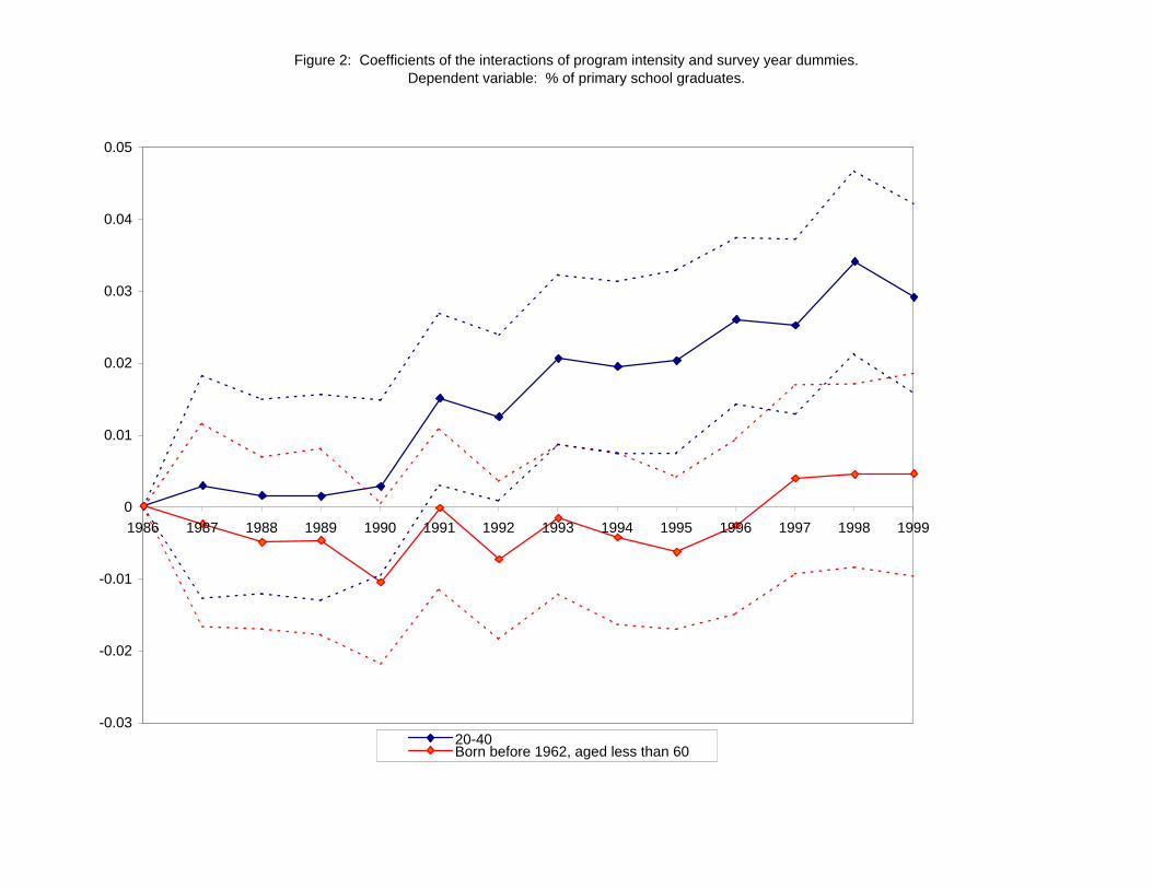
Since the generations exposed to the program have already started entering the sample in 1986,
one would expect all the coeÆcients of the interactions between program intensity and survey
year dummies to be positive and increasing. Columns 1, 2, 4 and 5 in table 2 show these
coeÆcients for the speci�cation that includes enrollment rates as a control, for adults aged
20 to 40, and for adults aged 20 to 60, in the whole sample and in a sample that excludes
urban districts.4 The fraction of \young" (or exposed) people among individuals aged 20 to 40
increases faster than among those aged 20 to 60, and one would expect the coeÆcients to be
larger and more signi�cant in the former group. The group of individuals aged 20 to 60, however,
corresponds better to \the labor market", and will therefore be important in the second stage
of this analysis. The coeÆcients are increasing for both groups, they are jointly signi�cant, and,
as expected, they are larger in the group aged 20 to 40. They become individually signi�cant
from 1991 in the 20-40 group and from 1996 in the 20-60 group.
This pattern could have been caused by factors other than the increase in education due to
INPRES, for example by migration of educated workers into districts that received more IN-
PRES schools. If I had data from earlier years, it would be possible to use \pre-program" data
to test the identi�cation assumption that the increase in education levels over time would not
4The speci�cation without enrollment rates as a control is very similar, and is therefore omitted.
7
have been systematically di�erent in regions where a di�erent number of schools was built, even
in the absence of the program. No comparable survey was realized before 1986. If the pattern
was due to something other than the e�ect of the program on education, however, one would
see a faster (or slower) increase in the education over the years, even in the subsample of those
who were not exposed to the program (individuals born in 1962 or before). To check this, I esti-
mated a speci�cation similar to equation 1, with the fraction of primary school graduates among
individuals born in 1962 or before as the dependent variable. The coeÆcients are presented in
columns 3 and 6 in table 2. Figure 2 gives a graphical summary of these estimates: It shows
the coeÆcients (and their con�dence intervals) for the entire group aged 20 to 40, and for the
group of individuals born before 1962. There is no systematic increase among the group born
before 1962. The coeÆcients in the two equations are signi�cantly di�erent from each other.
This indicates that the increase in average education is likely due to the program, rather than
to other factors.
2.4 Does migration undo the e�ect of local infrastructure development?
Although migration ows were not very important in Indonesia over the period, they are far from
negligible. In 1995, if one excludes Jakarta, 12% of individuals in the SUPAS sample did not
live in their province of birth, and 24% did not live in their district of birth (17% if one excludes
the urban districts). Among individual born in 1962, 13% did not live in their province of birth,
and 25% did not live in their district of birth. It is therefore interesting to study whether out
migration of educated workers dampened the e�ect of the program on average education in the
labor market.
The results in the previous section already suggest a partial answer to this question. The
program a�ected the average education of adults, which indicates that its e�ects were not totally
undone by migration. We can, however, make this result more precise by comparing the e�ect
the program should have had, in the absence of any o�-setting e�ect of migration, with the e�ect
it actually had. The results from this exercise are important in the context of an increasing focus
8
on decentralization, notably in Indonesia. If local governments believe their communities are not
getting any bene�ts from investment in education because educated people migrate (with their
human capital), decentralization of school �nance may lead the public �nancing of education to
decline.5
To get at this question, I �rst estimated the e�ect of the number of INPRES schools con-
structed per capita in an individual's district of birth on the probability that an individual
completed primary school, for each cohort. To this end, I used the SUPAS 1995 data. The
SUPAS (Intercensal survey of Indonesia) is a sample of over 200,000 households. It is represen-
tative at the district level. It is conducted every 10 years by the Central Bureau of Statistics
of Indonesia. The survey collects the same information as the SAKERNAS (which it replaced
in 1995), as well as more information about household members, including their province and
district of birth. The sample for this analysis is men born between 1950 and 1972 (there are
152,989 individuals in the sample).
Using this data, I regressed a dummy indicating whether an individual completed primary
school on a set of district of birth �xed e�ects, cohort of birth �xed e�ects, and interactions
between the number of schools constructed in one's district of birth and year of birth dummies.
The equation estimated is identical to equation (11) in Du o (2001), except that it used the
primary school completion (instead of years of education) as the dependent variable. Denote
the estimated e�ect of the program on the cohort born in year k as �̂k. I used the 1995 data
to compute the proportion of primary school graduates among those aged 20 to 40 in each year
(from 1986 to 1999) born in each district before 1962. Denote this average by gSoj. For each
survey year t and year of birth k, denote by �kt the share of those aged 20 to 40 who were born
in year k.6 We can then compute the proportion of primary school graduates predicted by the
program in each district and each year as:
5Bound, Kzedi and Turner (2000) ask the same question for college education in the U.S.6All the individuals who are born in 1962 or before are in the same cohort k.
9
fSjt =gSoj + Pj
t�20X
k=1962
�̂k�kt
!(2)
Note that this predicted value does not contain any information speci�c both to the district
and the year considered. There is therefore no source of mechanical relationship between fSjt andSjt. The �rst observation is that fSjt and Sjt are strongly correlated. The regression of the actualshare of primary school graduates on the predicted share leads to a coeÆcient of 0.84 (with a
t-statistic of 77). This, however, is not very informative, because a large part of this correlation
is driven by those born before 1962, and would therefore still exist even if all the educated young
had migrated out of the high program districts. The following experiment is more informative.
I run the same speci�cation as in equation 1, but I use as the dependent variable the predicted
education, fSjt. These coeÆcients indicate how the average education of adults would have been
a�ected in each region in the absence of any o�setting e�ect of migration. The coeÆcients
1l obtained in this speci�cation are plotted in �gure 3, along with the coeÆcients obtained
when estimating equation 1 with the actual average as the dependent variable. The two sets
of coeÆcients are surprisingly close to each other. In particular, there is no evidence that the
predicted e�ect is bigger than the actual e�ect.
3 Identifying the e�ect of a change in average education
3.1 Conceptual framework
Consider an economy with two sectors. Assume that there are only two types of workers,
educated (with a primary education or more) and uneducated (no primary education). Assume
that the formal sector employs educated labor, uneducated labor, and capital, and the informal
sector employs educated and uneducated labor and land.7 Individuals are self-employed in the
informal sector, and receive a wage in the formal sector. As in Harris and Todaro (1970) and
7I could allow land and capital to present in both sectors, but we would have to model migration of capital
and land between sector, for which I have little data.
10
other dual economy models of development, economic growth happens as the formal sector
expands. This is re ected in the assumption that land is a �xed factor. The share of the labor
force employed in the formal sector and their wages are the two variables of interest.
The production functions in the formal and informal sectors are given by f(AF ; EF ; UF ;K)
and g(AI ; EI ; UI ; T ) respectively, where K and T are the stock of capital and land respectively,
EF and UF denote educated and uneducated labor employed in the formal sector, respectively,
EI and UI denote educated and uneducated labor employed in the informal sector, and AF and
AI are \productivity" parameters. We will treat the total population as a constant (nothing is
a�ected by allowing steady population growth). The wages, as well as the fraction of educated
and uneducated workers working in each sector, are determined jointly in equilibrium as a
function of the number of educated and uneducated workers (in the economy as a whole), the
stock of capital, the stock of land, and the parameters AF and AE .
Normalizing the entire labor force to 1, and denoting S the share of educated workers, we can
therefore write the wage and formal employment functions as:8 ln(wE) = �E(AF ; AI ;K(S); S; T ),
ln(wu) = �U (AF ; AI ;K(S); S; T ), EF = E(AF ; AI ;K(S); S; T ), and UF = U (AF ; AI ;K(S); S; T ):
K is explicitly written as a function of S, to re ect the fact that a change in the proportion
of educated workers has a direct e�ect (the e�ect of the share of educated workers on the wage),
and an indirect e�ect due to the accumulation of physical capital in response to this increase.
The elasticity of physical capital with respect to the share of educated labor is an empirical
question: in the long run, one might expect the physical capital to adjust to a change in the
fraction of educated workers, while in the very short run, adjustment will be much more limited.
In the \medium run", the speed of adjustment of the capital stock will depend on the exibility
of the production function and the availability of �nance for the installation of new capital.
Consider a Taylor expansion of the wage function around S = 0.
Subject to the caveats discussed in the previous sub-section, we can use the number of
INPRES schools (Pj) as an instrument for Sjt � Sjt�1 in equation 8, possibly after controlling
for variables such as the enrollment rate and the wage in 1986 (a vector Cj). We have veri�ed
that Pj is uncorrelated with (Sjto � Sjt�1o), which is now included in the error term.
A joint test of the validity of the strategy and the seriousness of the problem suggested by
Acemoglu and Angrist (2000) is to use as dependent variable the average of the residual of a
regression of individual wages on individual education. If this equation is correctly speci�ed, it
15
should lead to the similar, but more precise estimate (since (Sjto � Sjt�1o) will not be part of
the error term any more).
Thus the reduced form with two years of data would be written:
ln(wjt)� ln(wjt�1) = �t + 2Pj + Æ2Cj + �jt
This equation can be generalized to incorporate all available years, leading to a reduced form
equation similar to equation 1:
lnwjt = �t + �j +1999Xl=1987
(�l � Pj) 2l +1999Xl=1987
(�l � Cj)Æ2l + �jt; (9)
where �t and j are year and district �xed e�ects, respectively.
Equations 1 and 9 form respectively the �rst stage and the reduced form of an instrumental
variables strategy to estimate equation 7.
The same reasoning applies to formal labor force participation, and the same speci�cation
can be estimated with formal labor force participation instead of wages. Finally we can also
estimate equations similar to equation 7, using the average skill premium as dependent variable.
The variables I consider here (wages, education, skill premium, formal labor force participation)
are likely to be auto-correlated over time. Bertrand, Du o and Mullainathan (2001) show that
this can cause severe downward bias in the estimated standard errors. I thus correct standard
errors in all equations using a generalization of the White variance formula which allows for a
exible auto-correlation process within any states.
Since the sample of individuals not a�ected by the program is di�erent every year, this
speci�cation may su�er from sample selection. First, the program may have induced selective
migration by old people, potentially correlated with their productivity, and therefore with their
wages. Second, I will show that the program a�ected the proportion of old people who work
for a wage: it also opens some room for selection bias, since it is possible that workers with the
lowest productivity switched to the wage sector. Section 4.5 will present additional evidence
(using two other data sets) on whether these two possibilities for sample selection a�ected the
16
results.
4 Results
Summary statistics for the sample of people born before 1962, and aged 60 or less in the survey
year, are presented in table 3. The proportion of primary school graduates among them increased
from 59% to 74% between 1986 and 1989 (this re ects the fact that individuals present in the
sample belong to later cohorts in later years). We determine participation in the formal sector
by noting whether an individual receives a wage. This fraction is a little over 30%. The average
wage, in real terms, increased by about 50% between 1986 and 1997, and declined by 22%
between 1997 and 1999.
4.1 Reduced form results
The reduced form results (the estimates of the coeÆcients 2l in equation 9) are presented in table
4 and in �gures 4A and 4B. These two �gures summarize the reduced form e�ects on wages and
on formal employment. Although none of these coeÆcients is individually signi�cantly di�erent
from zero, the reduced form coeÆcients in the wage equation are declining (in contrast to the
coeÆcients of average education, which are increasing). The reduced form coeÆcients on the
probability of working for a wage are increasing. In the sample that includes both urban and
rural areas, the coeÆcients increase from 1997 to 1999, which probably re ects the di�erential
impact of the crisis. In the rural sample, they are monotonically declining.
4.2 The e�ects of average education on wage rates
The main sample for the analysis is all the individuals aged 20 to 60 who were born before
1962.10 I will consider two independent variables. First, the fraction of primary school graduates
in the sample aged 20 to 60 (a reasonable approximation of the average education in the labor
10It means that, for each survey year, there is both a cohort e�ect and an age e�ect. I have run all the
speci�cations in a sample which maintains a constant cohort composition, and the results were very similar.
17
market); second, the fraction of primary school graduates among the 20 to 40 sample. The
INPRES program directly a�ected the latter (since the older a�ected people were 37 in 1999).
The former was a�ected as a consequence: Focusing on the 20-40 variable puts more accent on
the source of identi�cation.11 The results presented here focus on the share of primary school
graduates among males. Using instead the share of primary school graduates among males and
females combined leads to almost identical results.
Table 5 presents OLS estimates for equation 7, where the dependent variable is the average
wage and the average of the residual wage (after controlling for individual education and age).
The �rst panel does not include district �xed e�ects, while the second one does. As expected,
results obtained from speci�cations that do not control for individual education are bigger.
They lump together the \social" and the \private" returns. We should, therefore, focus on the
coeÆcients of average education in the wage residual equation. The di�erence between the �rst
and the second panel illustrates the remark made in the previous section: the OLS estimates
are much bigger than the corresponding �xed e�ects estimates, which suggests that they are
very strongly upward biased: educational attainments are higher in regions where wages are
higher, but this is as likely to come from a relationship running from income to education as
from the opposite relationship.12 The OLS results are all positive and signi�cant, while the
OLS results with �xed e�ect are positive, but signi�cant only in the speci�cation that has the
proportion of primary school graduates among those aged 20 to 60 as the dependent variable.
These point estimates suggest small positive e�ects: an increase of 10 percentage points in the
share of primary school graduates among those aged 20 to 60 is associated with an increase of
11In addition, the �rst stage is stronger for this variable, which minimizes the problems that can arise from
using weakly correlated instruments. One would expect the results with the 20-60 average to be a scaled up
version of the results obtained with the 20-40 average.12There are many reasons, besides those emphasized here, which would lead OLS coeÆcient to be biased
upwards. First, there may be a wealth e�ect in education: Glewwe and Jacoby (2000) �nd an important wealth
e�ect in Vietnam. Second, with economic growth, expected returns to education improve, and this may lead to a
higher demand for education (see Foster and Rosenzweig (1996) for micro-economic evidence of the Indian green
revolution, and Bils and Klenow (2000) for a re-interpretation of the cross-country evidence along these lines).
18
0.8% in the wages, after controlling for individual education. These coeÆcients are less than
one tenth of those estimated by Moretti (1999) for the impact of the share of college graduates
in the US.
Table 6 presents the instrumental variables results. The results are presented for the entire
sample, and for a sample that excludes the years 1998 and 1999, since the crisis hit di�erent
regions di�erently. The �rst line of each panel presents the results on wages. In the full sample,
the estimates become more negative when the crisis years are removed, while the estimates are
not a�ected in rural areas. The second line presents the results using the residual wages as
the dependent variable. None of the estimates is signi�cant. The estimates obtained using the
residual wage or the actual wage as the dependent variable are very similar, which is reassuring:
Since the INPRES instruments a�ects only average education, and not individual education,
controlling for individual education should not a�ect the estimate, which is what we �nd here.
The estimates using the residual wage are somewhat more precise. They suggest that an increase
of 10 percentage points in the share of primary school graduates among the 20 to 60 year old
led to a decrease of 3.8% in wages in the full sample, and to a decrease of 9.9 % in the sample
of rural areas. Without using the last two years of data, the coeÆcients are respectively -4.4%
and -9%. The negative coeÆcients are signi�cant (at the 10% level) in the rural sample only.
Focusing on the share of primary school graduates among the 20 to 40 year olds (for which
the �rst stage has more explanatory power), the story is the same: an increase of 10 percentage
points in the share of primary school graduates leads to a decrease of 2.9 % in the wage of the
old in the full sample, and to a decrease of 6.3% in the rural sample.
4.3 Skill premium
The third line in panel A and B of table 5 presents the results of estimating by OLS (with and
without district dummies) an equation similar to equation 7, but where the dependent variable is
the di�erence between the average wages of educated and uneducated workers. Without district
dummies, the estimate is negative, large (about -0.45), and signi�cant. With district dummies,
19
the estimates are negative, but much smaller (about -0.09) and insigni�cant. OLS seems again
to be biased upwards (in absolute value).
The third line in panels A and B of table 6 presents the instrumental variables estimates
of the same equation. The IV estimates of the e�ect of the share of primary school graduates
on the primary education premium are either negative or positive, and always insigni�cant.
The education premium does not seem to have been a�ected by the increase in the number of
primary school graduates. This suggests that, in at least one sector of the economy, educated
and uneducated workers are close substitutes.
4.4 Formal labor force participation
The fourth line in panels A and B of table 6 presents the instrumental variables results for formal
labor force participation (corresponding OLS results are presented in table 5). The dependent
variable is the fraction of people who work for a wage. The 2SLS estimates suggest that there
is a strong positive e�ect of the fraction of primary school graduates on the probability that
someone works for a wage. In the rural and urban sample combined, a 10% increase in the
proportion of primary school graduates among the 20 to 40 year old leads to a 4.5% increase
in the probability of working for a wage. A 10% increase in the proportion of primary school
graduates among the 20 to 60 year old leads to a 6.6% to 7.5% increase. The coeÆcients are
signi�cant in all of the speci�cations, and are very similar across speci�cations.
4.5 Sample selection
There are two possible sources of sample selection. First, there might be selective migration.
Second, since the program a�ected the proportion of people for whom we observe wages, the
probability of selection in the sample is a�ected by the instruments. In particular, one can
imagine a situation where the program pushed the \marginal" self-employed into the formal
labor force, and these marginal employees receive a lower wage. Moreover, new entrants into
20
the labor force have less experience, which should lower their wages.
Figure 2 (and columns 3 and 6 in table 4) suggest that the average education of individuals
born before 1962 in the sample was not a�ected by the program: along this observable dimension,
the sample remains comparable over time. Likewise, when I regress the education level of
individuals who were born before 1962 and who earn a wage on the interactions between the
program intensity and the survey year dummies, there is no distinct pattern in this regression
(the F statistic of the interactions is 1.03), which indicates that, along observable characteristics
at least, the composition of the formal labor force did not change as a result of the program.
However, there may have been selective migration along unobserved dimensions (if low pro-
ductivity old people are attracted to the program regions for example, or if high productivity
old people leave the region), which will cause a downward bias in the e�ect of the program on
wages. The SAKERNAS data does not indicate whether an individual is a migrant, and I do
not have any income measure for individuals who are not working for a wage. We thus need
other sources of information to shed light on this issue.
First, the SUPAS data set (the 1995 intercensal survey of Indonesia described earlier) has
the individual's region of birth as well as his region of residence. To investigate whether there
are di�erences in productivity between migrants and non-migrants that are correlated with the
INPRES program, I form for each district the di�erence between the logarithm of the hourly
wage of the migrants and that of the non-migrants (among those born before 1962 currently
residing in the district). Column 1 of table 7 presents a regression of this variable on the number
of INPRES schools built per capita in the region. The coeÆcient on the number of schools is
actually positive (but insigni�cant), which suggest that there is no downward sample selection
bias. In column 2, I construct the di�erence between the wage of those who migrated out of their
region of birth and those who stayed. This di�erence is unrelated to the level of the program.
There is thus no evidence that selective migration is likely to bias the results downward.
Second, I use the SUSENAS data (a nationally representative survey of about 50,000 house-
holds, which has an income and a consumption supplements once every 5 years). I use the
21
incomes modules from the SUSENAS from 1987 and 1993 to compute the ratio of the house-
hold income of self employed to the household income of wage earners. The ratio is very stable
between 1987 and 1993: self-employed earn 17.85% less than employed in 1987, and 18.5% less
in 1993. I then regress the di�erence in the log of this ratio (table 7, column (3)) on the level of
the program, and found no relationship (the coeÆcient of the INPRES program is 0.0021, with
a t-statistic of 0.130).
On balance, it appears that the relative wage loss of the old generation in regions where the
program increased the supply of primary school graduates cannot be attributed to a composition
e�ect.
We can summarize the results from this section as follows. An increase in the share of the
educated workers leads to:
� A decline in the wage of older workers, whose level of education did not change. The
point estimate is large (as large as the skill premium itself, or even larger in rural areas),
although it is signi�cant only in some speci�cations.
� No change in the skill premium among older workers.
� An increase in the share of the labor force employed in the formal sector, among the old.
The point estimates are large (a 10% increase in the share of educated workers leads to
an increase of at least 4% in the share of old workers employed in the formal sector) and
signi�cant.
� No change in the di�erence between formal and informal sector earnings.
In the next section, I build a model which can explain these e�ects, and serve as a framework
to interpret their magnitude.
22
5 Model and interpretation
What do these results tell us about the the response of the economy to an increase in the
education of the labor force? In this section, I use a simple two-sector model as a framework
to interpret these e�ects and their magnitude. In the �rst subsection, I set up the model and
study the e�ect of education on wages and the allocation of labor across sectors, taking capital
as given. In the second subsection, I compare the predictions of the model to the data. I specify
two polar cases for the accumulation of capital. In the �rst case, there is no adjustment cost. In
the second case, physical capital accumulation does not adjust at all to changes in the rate of
human capital accumulation. In this simple model, both assumptions have the same implication
for formal labor force participation, but very di�erent implications for wage rates.
Below, I provide some justi�cation for the speci�c assumptions of the model.
The fact that the skill premiumwas not a�ected suggests that, at least in one sector, educated
and uneducated workers are very strong substitutes. Since in the formal sector, workers are
combined, while they are self employed in the informal sector (we can think about this sector as
small scale agriculture), we will take as a starting point that educated and uneducated workers
are perfect substitutes in the informal sector. Suppose that the informal sector combines land
and human capital, and the formal sector combines physical and human capital. The informal
sector is characterized by a downward sloping demand for e�ective units of labor, even in the
long run (because land is a �xed factor). In the formal sector, the slope of the labor demand
depends on how capital adjusts to changes in the composition of the labor force. If capital does
not adjust to an increase in e�ective labor supply, labor demand will be downward sloping. It
would be at if this increase led to an o�setting increase in the supply of capital, or even slope
upwards if there were technological externalities, or if faster capital accumulation more than
o�set human capital accumulation (as in Acemoglu (1996)).
Consider a simple competitive model, where wages are equalized in the formal and informal
sector (for a given level of skill). Figure 5 illustrates the e�ect of the increase in educated workers
induced by the INPRES reform on uneducated old workers. The total number of old uneducated
23
workers and their allocation between the formal and the informal sector are depicted on the X
axis. The left Y axis presents the wage in the formal sector, and the right Y axis presents
the wage in the informal sector. The increase in the number of educated workers leads to a
shift in the labor supply expressed in eÆciency units, which is akin to a shift to the right of
the labor demand in the informal sector, and a shift to the left in the formal sector. If the
labor demand in the formal sector is downward slopping, the e�ect on wages is unambiguously
negative. The e�ect of an increase in the number of educated workers on the allocation of labor
between formal and informal sector depends on the ratio of the elasticity of substitution between
capital and labor in the formal sector and that between land and labor in the informal sector.
The observation that the increase in the proportion of educated workers led to a shift from
the informal to the formal sector indicates that the elasticity of substitution between labor and
capital is bigger than the elasticity of substitution between labor and land. We will capture this
with the simplifying assumption that the informal sector uses a Leontie� technology.
5.1 Model
This section builds a speci�c model along the lines described above. We start by describing
the allocation of labor and the determination of wages, taking capital as given. In the second
subsection, I will compare the predictions of this model to the data, using two polar cases for
the adjustment of capital to the increase of the share of educated workers: no adjustment cost,
vs. no adjustment whatsoever (in�nite adjustment costs).
There is a mass 1 of workers in the economy, a fraction S of which are educated. There are
two sectors, an informal (small scale agriculture) and a formal sector (industry).
Suppose that the informal sector is characterized by a Leontie� production function in terms
of eÆciency units:
YI = Min(T;HI);
where HI is the number of eÆciency units employed in the informal sector, and T is the (nor-
malized) amount of available land.
24
In addition, assume that educated and uneducated workers are perfect substitutes in the
informal sector:
HI = UI + hEI ;
where h is the relative eÆciency of educated workers. Land is distributed optimally between
educated and uneducated workers, and both earn their marginal productivity, so that the ratio
of the educated to the uneducated wage is h.
The production function in the formal sector is Cobb-Douglas in human and physical capital,
with constant returns to scale:
YF = AFK�H1��
F
Human capital is a Cobb-Douglas aggregate of educated and uneducated workers:
HF = E�FU
1��F
Wages in the formal sector are given by the marginal productivity of each factor:
wEF = (1� �)AFK�H��
F �E��1F U
1��F ;
and
wUF = (1� �)AFK�H��
F (1� �)E�FU
��F :
In equilibrium, the ratio wEFwUF
must be equal to h. Therefore the ratio of uneducated to
educated labor in the formal sector must satisfy the relationship:
UF
EF= h
1� �
�(10)
Together with the relationships EF + EI = S, UF + UI = 1 � S and hEI + UI = T , this
determines the employment of each category of workers in each sector:
EF =�
h[1 + S(h� 1)� T ] (11)
EI =�
h[T � 1� S(h� 1) +
h
�S] (12)
UF = (1� �)[1 + S(h� 1)� T ] (13)
UI = T � �[T � 1� S(h� 1) +h
�S] (14)
25
Production in the formal sector can be expressed as a function of EF :
YF = AF
�h1� �
�
�1��!1��
K�E1��F
The wage of an educated worker is therefore given by:
ln(wE) = C + � ln(K)� � ln(EF ) ; (15)
ln(wE) = C 0 + � ln(K)� � ln(1 + S(h� 1)� T ) ; (16)
where C and C 0 are functions of �, �, AF and h.
The same equations (with di�erent C and C 0) describe the wage of an uneducated worker.
5.2 Calibration
5.2.1 E�ect of education on formal employment
The ratio of educated to uneducated workers in the formal sector, divided by the skill premium,
should be constant, according to our model, and allows us to calculate �. In fact, the ratio of the
number of uneducated workers to the number of educated workers is decreasing over time (table
1, column 5), while the skill premium is stable (table 1, column 6). The value of � obtained
from equation 10 is therefore increasing. This may re ect factors not taken into account, such
as the adoption of more skill-complementary technologies. The average value of � is 0.62.
Equations 11 and 13 indicate how employment of educated and uneducated workers in the
formal sector responds to a change in S. Suppose that all the newly educated workers are
\born" into the informal sector, and that young and old workers shift from the informal to the
formal sector to restore the correct proportion between EF and UF . When S increases by 1%,
the probability that an educated worker born before 1962 will be employed in the formal sector
increases by �h(h�1)So
, and the probability that an uneducated worker born before 1962 will be
employed in the informal sector increases by (1 � �) (h�1)1�So
, where So is the share of educated
workers among the old.
26
Values of the parameters �, h and So are shown in tables 1 and 3. The average value of h�1
(the skill premium) is close to 0.40. The average value of So is around 0.65. The model would
therefore predict that an increase in S of one percentage point would make the educated and
uneducated born before 1962, respectively, 0.29 percent and 0.41 percent more likely to work in
the formal sector.
The coeÆcients we have estimated suggest that an increase in S of one percentage point leads
to an increase in the probability of working for a wage of 0.43 (in the combined sample) and
0.71 (in the rural sample) for the educated workers. For the uneducated workers, the estimated
e�ects are respectively 0.51 (in the combined sample) and 0.31 (in the rural sample). Therefore,
the model does a reasonable job in predicting the shift from the informal to the formal sector
for the uneducated, and under-predicts the shift of the educated from the formal to the informal
sector, especially in the rural sample.
5.2.2 E�ect of an increase in average education on wage rates
The e�ect of the increase in average education on the wages (at a given level of human capital)
depends on the extent to which physical capital adjusts to the increase in human capital. We
contrast the implications of two polar cases. In the �rst case, capital adjusts costlessly to
the modi�cation induced by INPRES: I �rst consider the situation where each district is a
closed economy with local accumulation, and then a situation where capital is freely mobile
across regions. Both models deliver the results that wage growth across regions should not be
di�erentially a�ected. In the second case, there is no adjustment at all of the physical capital
stock in response to the INPRES program, over the period under consideration.
� Costless capital stock adjustment, local capital accumulation
To study the consequences of the INPRES model in the case of costless adjustment, we
need to specify how human capital and physical capital are accumulated. Following Barro and
i Martin (1995) (chapter 5), consider a one-sector endogenous growth model, with human and
physical capital. Output is divided between consumption and investment in the two forms of
27
capital.
Y = AFK�H
(1��)F + T = C + IK + IH ;
where IK and IH are the gross investment in physical and human capital, respectively.
The changes in the capital stocks are given by:
_K = IK � ÆK;
and
_HF = �IH(t� L)� ÆHF :
Note two di�erences from the set up in Barro and i Martin (1995). First, there is a lag of
duration L between investment in human capital and the date at which it will become active:
this re ects the fact that children who go to school today will enter the job market only after
a lag. Second, � represents the ratio at which each unit of investment is transformed into a
unit of human capital.13 Note that H could not accumulate inde�nitely if the only way to
increase H were to increase the proportion of primary school graduates. We should think of H
as a Cobb-Douglas aggregate of all levels of education: I model the beginning of the process of
development, where only two levels of education have been achieved.
The solution to this problem is obtained by setting up the Hamiltonian expression for the
household choice between consumption and investment in human or physical capital, taking �rst
order conditions with respect to C, IH , IK , K and HF . The steady state growth rate is equal
to:
=1
�
"AF�
�K
HF
���1
� Æ � �
#
The steady state value of KHF
is pinned down by the condition of equality between net returns
to investment in physical and human capital. It is the solution to the following implicit equation:
13In the dual economy model, � re ects both the cost of producing educated workers, and the rate at which
the educated workers are participating in the formal labor market.
28
�eL
���AF
�K
HF
���1� �
K
HF
��=
�
1� �; (17)
Denote k� the value of KHF
given by this equation. The steady state growth rate is given by:
� =1
�
hAF�k
�(��1)� Æ � �
i(18)
We can model the e�ect of the INPRES program as an increase in �, the rate at which
investment is transformed into human capital accumulation: each new school makes it cheaper
to accumulate human capital. Suppose that the INPRES program will last long enough that we
can think about it as a permanent program (a permanent increase in �).14 In the new steady
state, the ratio k� will be lower than in the old steady state, to maintain the equality between
net returns to investment in human capital and physical capital (see equation 17). The program
should therefore cause a drop in the levels of wages (holding human capital constant). After the
transition, consumption, human capital and physical capital will grow at the same new steady
state rate (given by equation 18). In the new steady state, growth in human capital will be
exactly matched by growth in physical capital, and wage growth will therefore be una�ected by
growth in human capital. To see this, di�erentiate equation 15 with respect to time, and note
that_KK=
_HFHF
, so that the two terms cancel.
The transition to the new steady state involves indeed a decline of KHF
, and therefore a
decline in wages. In this model, however, the adjustment in the ratio KHF
should have taken
place right after the program was initiated, and well before the rate of growth of H actually
starts to accelerate. To see this, imagine that the economy were initially at a steady state, and
consider the household decision the �rst day the schools are built: human capital investment has
suddenly become cheaper, while physical capital investment has the same price and the same
returns as before (since the human capital available today keeps growing at the old steady state
growth rate). Net returns to investing in human capital are therefore higher, all the investment
14For our purpose, it would not be easy to distinguish a permanent temporary program, since the rate of capital
accumulation was more rapid in the regions that received more schools for the entire period under consideration.
29
takes the form of human capital, and the ratio KHF
declines rapidly until it is low enough that
investing in physical capital become pro�table again. Simulations of the transitional dynamics
of this model show that the ratio KHF
gets very close to its steady state value very fast after the
program is initiated (in one year if there if household are allowed to transform physical capital
into human capital, and in less than 3 years otherwise).15 Afterwards, the ratio KHF
stay almost
constant.16
This very fast adjustment rate may seem unrealistic, but this is because the assumption of
costless capital adjustment is not realistic either, even though it underlies, implicitly or explicitly,
the e�ort to identify a human capital externality (in which case the share of educated workers
could have a positive e�ect on wages). The important point is to note that in this model, the
share of educated workers should not a�ect wages from 1986 to 1999. The data do not seem
to support this full adjustment model for Indonesia, however: during the entire period, wages
grow more slowly in regions were human capital grows faster (see �gure 4B).
� Costless capital stock adjustment, national capital accumulation and freely mobile capital
across regions.
If capital is freely mobile across regions and there are no adjustment costs, the capital stock
simply adjusts to the increase in human capital to equalize the returns to physical capital across
regions. This determines the physical capital/human capital ratio k, which in turns determines
the wage: thus (absent positive externalities), the evolution of wages should not be di�erent in
regions that received more schools (the level of wages may of course be related to the program).
Once again, the data do not seem to support this model.
15For example, if 1 was initially 3.5% a year, assuming a value of 0.05 for Æ, K
HFwould have declined by 8%
every year. With reasonable parameters values for �, Æ, �, and � (� = 0:3, Æ = 0:05, � = 0:02, � = 3) , and
assuming that the e�ect of each school on the rate of growth of S we observe in the data is the steady state e�ect
(i.e. each school causes an increase of 0.5% in the growth rate), K
HFshould fall by about 10% for each school
built (per 1000 children), which would have been achieved in 1.25 years. On average, 2 schools were built, so in
2.5 years, K
HFshould have fallen enough in the average region to reach the new steady state value.
16In the simulations, there are small oscillations around the steady state values, and they are progressively
dampening.
30
There were more than 10 years between the start of the program and the entry into the labor
force of the generations that were exposed to it. Thus, even if capital accumulates with a gap
(\time to build"), the conclusions of such a model would be unchanged.
Thus, it seems that, to account for the pattern present of the data, it is necessary to introduce
frictions in the adjustment of the capital stock. We consider an extreme case of frictions.
� No adjustment of the capital stock in response to the increase in education
The other extreme is a case where there is absolutely no response of physical capital accu-
mulation to the increase in the stock of educated workers. The stock of capital thus evolves
exogenously. In this case, if the INPRES program is a valid instrument (that is, if it is not
correlated with the exogenous rate of capital accumulation), the stock of capital enters the error
term in equation 15 and is uncorrelated with the level of the program. The best way to check
whether our model �ts the facts is to use ln(EF ) or ln(1+S(h�1)�T ) as the dependent variable
instead of S.17 Figure 6 shows that these variables are also in uenced by the program. The
�rst stage coeÆcients for these two variables are similar, which is reassuring.18 The �gure also
looks similar to �gure 2. In table 8, I present the results of estimating equation 15, using the
same strategy outlined for estimating the e�ect of S on wages. In practice, I estimate equation
7, with ln(EF ) or ln(1 + S(h� 1)� T ) as the endogenous regressor of interest.
The coeÆcients of a subset of the speci�cations estimated in table 6 are presented in table 8.
For ln(EF ) (columns (1) and (2)), the pattern is similar to what we found for S: the coeÆcients
are negative, but insigni�cant. The point estimate is -0.07 in the urban sample, and -0.22 in the
rural sample. The latter estimate of -0.22 is close to -0.3, the conventional guess for �.
The results using ln(1+S(h�1)�T ) as the independent variable are more encouraging. The
point estimates are similar in the combined sample and in the rural sample. The estimates range
17ln(EF ) is the proportion of the labor force that is educated and works in the formal sector. ln(1+S(h�1)�T )
is calculated using the district and year-speci�c skill premium. T is calculated using its de�nition: T = HI =
UI + h �EI .18I estimate the same speci�cation as in equation 1, but I use lnEF and ln(1 + S(h� 1) � T ), respectively, as
the dependent variables. Full results are presented in table A1.
31
between -0.34 and -0.40, and are all signi�cant at the 10% level of con�dence (after correcting
the standard errors for auto-correlation over time within regions). These estimates (especially
those obtained in the combined sample) are higher than what I obtained using ln(EF ) (they
should in principle be the same). They are very close to (and not signi�cantly di�erent from)
-0.3. These estimates are fairly precise and their order of magnitude is reasonable.
Note that the model predicts that the e�ect of the program on wages should be the same in
the formal and in the informal sector. The SAKERNAS does not have data on income for those
who do not work for a wage. However, the regression in column 3 of table 7, discussed in section
4.5, suggests that the ratio of the income of the wage earners to that of non-wage earners was
not a�ected by the program: the di�erence between the value of this ratio in 1993 and in 1987
is not correlated at all with the intensity of the program.
This set of estimates therefore suggests that the accumulation of physical capital happens
essentially independently from the accumulation of human capital. Even 25 years after the pro-
gram was initiated, physical capital does not seem to have been accumulated to employ the new
eÆciency units of labor created by the program. This conclusion seems consistent with other
evidence on the pattern of industrialization in Indonesia during the period. After 1984, the
Indonesian Government cut all previously existing tax incentives to geographical dispersion and
small businesses Hill (1996). Miguel et al. (2001) show that there was divergence in industri-
alization across regions between 1985 and 1995: industrialization was faster during this period
in regions where its level was higher in 1985. Moreover they show that change in the rate of
industrialization seem uncorrelated with school construction (not only INPRES schools, but all
primary and junior high schools) in the previous decade, as well as with other infrastructure
variables (roads or electricity).
6 Conclusion
This paper argued that the INPRES program, a large school construction program undertaken
by the Indonesian government in the 1970's, constitutes a good case study to empirically examine
32
the impact of average primary schooling on the wages of older cohorts. This program modi�ed
the enrollment rates of the young generations, thus inducing a long-lasting change in the rate of
human capital accumulation in the regions it a�ected most. We can study impact of this shock
on the supply of educated workers on an \old" generation that did not directly bene�t from the
program. It provides a natural solution to the identi�cation problems inherent to any attempt
to identify the e�ect of the average of a regressor while trying at the same time to control for it.
The instrumental variables estimates presented in this paper suggest that the e�ect of average
education on individual wages (holding skill level constant) is negative: in places where average
educational attainments grew faster because of the program, wages grew more slowly. This
does not seem to be due to sample selection bias due to migration or increases in labor force
participation. This is in sharp contrast to the OLS estimates, which are strongly positive, and
to the �xed e�ect estimates, which are closer to zero but still positive. Such a strong bias in
the OLS estimates suggests that the cross-country relationship between output per capita and
education is likely to be a�ected by the same upward bias. The e�ects of average education on
the participation in the formal labor market is, however, positive.
Both sets of estimates are shown to be consistent with a simple dual-economy model, where
the number of eÆciency units that can be productively employed in the informal sector is limited
by the availability of a �xed factor (land, for example). The increase in the productivity of the
labor force is entirely absorbed by the formal sector, which explains the increased participation.
Wages decrease to the extent that physical capital does not fully adjust to the increase in human
capital. I contrast three versions of this model. In a closed economy endogenous growth version
with costless adjustment of the capital stock, the faster increase in human capital after 1986
should be matched with a corresponding increase in the stock of physical capital, and wages
should be una�ected. In an open economy model where capital moves freely, the capital-labor
ratio adjusts to maintain equal returns to physical capital across regions, and the program
should have no e�ect on wages. If capital accumulation is unresponsive to the increase in human
capital, the predicts that the coeÆcient on the human capital variable should be the negative
33
of the elasticity of production with respect to capital.
The extent to which wages fall in response to the increase in human capital available in the
formal sector suggests that there was little or no reaction of the physical capital to the increase
in educational opportunities in the regions where INPRES built more schools. The estimates I
obtain are reasonable if this is the right model of the world.
What is absent in this paper (and left for future work) is an explanation of why the capital
stock did not adjust. The program was publicly announced, and the increase in the stock of
primary school graduates occurred gradually over 10 years after the program started. It is a
puzzle that 25 years after the program was initiated, the labor demand looks like a \short run"
labor demand curve. Future work (and, probably, more data) is needed to determine to what
extent this is due to \myopic" behavior of investors, who fail to recognize the increase in the
education level of the labor force, very large adjustment costs of the capital stock, to a �nancing
constraint, or a combination of the three.
The results in this paper are important because, contrary to what is often assumed (on the
basis of the experience of South-East Asian countries), acceleration in the rate of accumulation of
human capital is not necessarily accompanied by economic growth. Several countries (in Africa,
in particular) had very rapid expansion in education, but dismal economic growth (Kremer and
Thomson (1998)). It is important to understand why this can be the case.
Models of credit constraints (Banerjee and Newman (1993), Galor and Zeira (1993), Aghion
and Bolton (1997)) could be combined with models of costly adjustment of technology to study
the e�ects of education on economic growth given the actual constraints faced by developing
economies. The work of Caballero and Hammour (1998, 2000) comes closest to doing this. Their
model combines costly adjustment with credit constraints but does not model growth. It cannot
therefore be directly applied to the question of what happens when the growth rate of human
capital increases. Once built, such a model could then be compared to actual evolutions, in
exercises similar to Blanchard's (1997) analysis of the \medium run".
34
References
Acemoglu, Daron (1996) `A microfoundation for social increasing returns in human cpital accu-
mulation.' Quarterly Journal of Economics 111(3), 779{804
Acemoglu, Daron, and Joshua Angrist (2000) `How large are human capital externalities? Evi-
dence from compulsory schooling laws.' NBER Macroannual, pp9-59
Aghion, Philippe, and Patrick Bolton (1997) `A trickle-down theory of growth and development
with debt overhang.' Review of Economic Studies 64(2), 151{72
Atkinson, Tony, and Andrea Brandolini (2001) `Promise and pitfalls in the use of \secondary"
data-sets:Income inequality in the OECD countries as a case study.' Journal of Economic
Litterature 39, 771{779
Banerjee, Abhijit, and Andrew Newman (1993) `Occupational choice and the process of devel-
opment.' Journal of Political Economy 101(2), 274{298
Banerjee, Abhijit, and Esther Du o (2000) `Inequality and growth: What can the data say?'
Working Paper 7793, National Bureau of Economic Research, July
Barro, Robert, and Xavier Sala i Martin (1995) Economic Growth (Mc Graw Hill)
Bertrand, Marianne, Esther Du o, and Sendhil Mullainathan (2001) `How much should we trust
di�erences in di�erences estimates.' Mimeo, MIT
Bils, Mark, and Peter Klenow (2000) `Does schooling cause growth or the other way around?'
American Economic Review 90(5), 1160{1183
Blanchard, Olivier (1997) `The medium run.' Brookings Papers on Economic Activity 2, 89{158
Blanchard, Olivier, and Justin Wolfers (2000) `The role of shocks and institutions in the rise of
european unemployment: The aggregate evidence.' Economic Journal pp. 1{33
35
Bound, John, Gabor Kzedi, and Sarah Turner (2000) `Trade in university training: Cross state
variation in the production and use of college educated labor.' MIMEO, University of
Michigan
Caballero, Ricardo, and Mohamad Hammour (1998) `The macroeconomics of speci�city.' Journal
of Political Economy 106(4), 724{767
(2000) `Creative destruction and development: Institutions, crises, and restructuring.'
Working Paper 7849, National Bureau of Economic Research, August
Card, David, and Thomas Lemieux (2001) `Can falling supply explain the rising return to college
for younger men? A cohort-based analysis.' Quarterly Journal of Economics 116(2), 705{
746
Du o, Esther (2001) `Schooling and labor market consequences of school construction in Indone-
sia: Evidence from an unusual policy experiment.' American Economic Review 91(4), 795{
813
Foster, Andrew D., and Mark R. Rosenzweig (1996) `Technical change and human-capital re-
turns and investments: Evidence from the green revolution.' American Economic Review
86(4), 931{953
Frankenberg, Elizabeth, Duncan Thomas, and Kathleen Beegle (1999) `The real costs of Indone-
sia's economic crisis: Preliminary �ndings from the Indonesia family life surveys.' Working
Paper 99-04, RAND Labor and Population Program
Galor, Oded, and Joseph Zeira (1993) `Income distribution and macroeconomics.' Review of
Macroeconomic Studies 60, 35{52
Glewwe, Paul, and Hanan Jacoby (2000) `Economic growth and the demand for education: Is
there a wealth e�ect?' MIMEO, World Bank
36
Harris, J., and M. Todaro (1970) `Migration, unemployment and development: A two-sector
analysis.' American Economic Review 40, 126{142
Heckman, James J., Lance Lochner, and Christopher Taber (1998) `General equilibrium treat-
ment e�ects: A study of tuition policy.' Working Paper 6426, National Bureau of Economic
Research
Hill, Hal (1996) The Indonesian Economy Since 1966: Southeast Asia's Emerging Giant (Cam-
bridge: Cambridge University Press)
Katz, Lawrence F., and Kevin M. Murphy (1992) `Changes in relative wages, 1963-1987: Supply
and demand factors.' Quarterly Journal of Economics 107(1), 35{78
Kremer, Michael, and James Thomson (1998) `Why isn't convergence instantaneous? young
workers, old workers, and gradual adjustment.' Journal of Economic Growth 3, 5{28
Krueger, Alan, and Mikael Lindahl (2001) `Education for growth: Why and for whom?' Journal
of Economic Literature
Lucas, Robert (1988) `On the mechanics of economic development.' Journal of Monetary Eco-
nomics 22, 3{42
Miguel, Edward, Paul Gertler, and David Levine (2001) `Did industrialization destroy social
capital in Indonesia.' Mimeo, U.C. Berkeley
Moretti, Enrico (1999) `Estimating the social return to education: Evidence from repeated
cross-sectional and longitudinal data.' Working Paper 22, UC Berkeley
Solow, Robert M. (2000) `Toward a macroeconomics of the medium run.' Journal of Economic
Perspectives 14(1), 151{158
Welch, Finis (1979) `E�ects of cohort size on earnings: The baby boom babies' �nancial bust.'
Journal of Political Economy 87(5), S65{S97. part 2
37
Table 1: Descriptive statistics
ratio of Skill Implied20-40 20-60 20-40 20-60 uneducated/educated premium beta
in formal sector (20-60)(1) (2) (3) (4) (5) (6) (7)
Notes: 1. Average wage is average of the log of monthly wage2-Means are weighted by the number of observations ineach district-year cell3. See text for the definition of Beta
Percentage of primary school graduatesFraction born after 1962
Table 2: First stage regressionsEffect of the program on the proportion of individuals completing primary school or more.
Coefficients of interactions of the intensity of the program and survey year dummies.
Sample: Born Born 20-40 20-60 before 1962 20-40 20-60 before 1962
Notes: 1. The program intensity is the number of INPRES schools built between 1974 and 1978, divided by thenumber of children in 1971.2. Survey year dummies, region dummies, interactions between survey year dummies and the enrollment rate in 1971, and interactions between suvey year dummies and the number of children are includedin the regressions.3. Regression run using kabupaten-year averages, weighted by the number of observations in each kabupaten-year cell.4. The F statistic is for the hypothesis that the set of interactions is jointly insignificant.5. The standard errors are corrected for auto-correlation within kabupaten.
Sample: Urban and rural areas Sample: rural areas only
Table 3: Descriptive StatisticsSample: individuals aged less than 60 and born before 1962
Survey year % primary school % working average S.D. of skillgraduates for wage wage wage premium
Notes: 1. The program intensity is the number of INPRES schools built between 1974 and 1978, divided by thenumber of children in 1971.2. Survey year dummies, region dummies, interactions between survey year dummies and the enrollment rate in 1971, and interactions between suvey year dummies and the number of children are includedin the regressions.3. Regression run using kabupaten-year averages, weighted by the number of observations in each kabupaten-year cell.4. The standard errors are corrected for auto-correlation within kabupaten.
20-60 years old, born before 1962 20-60 years old, born before 1962Sample: Urban and rural areas Sample: Rural areas only
Table 5: OLS estimates of the impact of average education on individual wages.Men aged 20-60 and born before 1962.
Sample: Rural Sample: Rural Sample: Rural Sample: Rural and urban areas areas only and urban areas areas only
(1) (2) (3) (4)
PANEL A: OLS, without region fixed effects (1986-1999)
Notes: 1. Survey year dummies, region dummies, interactions between survey year dummies and the enrollment rate in 1971, and interactions between suvey year dummies and the number of children are included in the regressions.2. Regression run using kabupaten-year averages, weighted by the number of observations in each kabupaten-year cell.
Independent variable: % of primary school graduates in the 20-40 sample
Independent variable: % of primaryschool graduates in the 20-60 sample
Table 6: 2SLS estimates of the impact of average education on individual wages.Men aged 20-60 and born before 1962.
Sample: Rural Sample: Rural Sample: Rural Sample: Rural and urban areas areas only and urban areas areas only
Notes: 1. Survey year dummies, region dummies, interactions between survey year dummies and the enrollment rate in 1971, and interactions between suvey year dummies and the number of children are included in the regressions.2. Regression run using kabupaten-year averages, weighted by the number of observations in each kabupaten-year cell.3. The instruments are interactions between survey year dummies and the program intensity4. The standard errors are corrected for auto-correlation within kabupaten.
school graduates in the 20-40 sample school graduates in the 20-60 sampleIndependent variable: % of primary Independent variable: % of primary
Program intensity 0.0229 0.011 -0.00207(0.0159) (0.0164) (0.0160)
Number of cells 285 288 272Note:
1. The program intensity is the number of INPRES schools built between 1974 and 1978, divided by thenumber of children in 1971.2. The formal sector premium is defined as : log(income of wage earner/income of non wage earners)3. The enrollment rate and the number of children in 1971 are introduced as controls in the regressions4. The data for columns (1) and (2) is the SUPAS 19955. The data for column (3) is the SAKERNAS, 1987 and 1993.
Table 8: 2SLS estimates of the impact of human capital on wages. log(Ef) and log(1+S(h-1)-T) as measures of human capital
Sample: Rural Sample: Rural Sample: Rural Sample: Ruraland urban areas areas only and urban areas areas only
Notes: 1. Survey year dummies, region dummies, interactions between survey year dummies and the enrollment rate in 1971, and interactions between suvey year dummies and the number of children are included in the regressions.2. Regression run using kabupaten-year averages, weighted by the number of observations in each kabupaten-year cell.3. The instruments are interactions between survey year dummies and program intensity4. The standard errors are corrected for auto-correlation within kabupaten.
Dependent variable: Log(wage) for men 20- 60, born before 1962Independent variable: log(EF)
among sample aged 20-60Independent variable: log(1+s(h-1)-T)
among sample aged 20-60
Figure 1 -- COEFFICIENTS OF THE INTERACTIONS OF AGE IN 1974* PROGRAM INTENSITY IN THE REGION OF BIRTH IN THE EDUCATION
EQUATION
-0.2
-0.1
0
0.1
0.2
0.3
234567891011121314151617181920212223
Age in 1974
Figure 2: Coefficients of the interactions of program intensity and survey year dummies.Dependent variable: % of primary school graduates.
Figure 3: Actual and predicted coefficients of the interactions of program intensity and survey year dummies.Dependent variable: % of primary school graduates.
20-40, actual coefficients 20-40, predicted coefficients
Figure 4A: Coefficients of the interactions of program intensity and survey year dummies. Dependent variables: log(wage) and formal sector employment (individuals born before 1962 and aged less than 60)
Figure 4B: Coefficients of the interactions of program intensity and survey year dummies. Dependent variables: average log(wage) and average formal sector employment among individuals born before 1962 and aged less than 60.
Notes: 1. The program intensity is the number of INPRES schools built between 1974 and 1978, divided by thenumber of children in 1971.2. Survey year dummies, region dummies, interactions between survey year dummies and the enrollment rate in 1971, and interactions between suvey year dummies and the number of children are includedin the regressions.3. Regression run using kabupaten-year averages, weighted by the number of observations in each kabupaten-year cell.4. The F statistic is for the hypothesis that the set of interactions is jointly insignificant.5. See text for variables definition6. The standard errors are corrected for auto-correlation within kabupaten.