Working Paper Series - Banco Central do Brasil · Working Paper Series ISSN 1518-3548 Speculative...

Working Paper Series

ISSN 1518-3548

Speculative Attacks on Debts, Dollarization and OptimumCurrency Areas

Aloisio Araujo and Márcia Leon April, 2002

ISSN 1518-3548 CGC 00.038.166/0001-05


Brasília

n. 40

Apr

2002

P. 1-74


Edited by: Research Department (Depep)

(E-mail: [email protected])

Reproduction permitted only if source is stated as follows: Working Paper Series n. 40. Authorized by Ilan Goldfajn (Deputy Governor for Economic Policy). General Control of Subscription: Banco Central do Brasil

Demap/Disud/Subip

SBS – Quadra 3 – Bloco B – Edifício-Sede – 2º subsolo

70074-900 Brasília – DF – Brazil

Phone: (5561) 414-1392

Fax: (5561) 414-3165

The views expressed in this work are those of the authors and do not reflect those of the Banco Central or its members. Although these Working Papers often represent preliminary work, citation of source is required when used or reproduced. As opiniões expressas neste trabalho são exclusivamente do(s) autor(es) e não refletem a visão do Banco Central do Brasil. Ainda que este artigo represente trabalho preliminar, citação da fonte é requerida mesmo quando reproduzido parcialmente. Banco Central do Brasil Information Bureau Address: Secre/Surel/Diate

SBS – Quadra 3 – Bloco B

Edifício-Sede – 2º subsolo

70074-900 Brasília – DF – Brazil

Phones: (5561) 414 (....) 2401, 2402, 2403, 2404, 2405, 2406

DDG: 0800 992345

Fax: (5561) 321-9453

Internet: http://www.bcb.gov.br

E-mails: [email protected]

[email protected]

Speculative Attacks on Debts, Dollarization andOptimum Currency Area∗

Aloisio Araujo † Márcia Leon ‡

AbstractThe purpose of this article is to contribute to the discussion of the financial aspects

of dollarization and optimum currency areas. Based on the model of self-fulfilling debtcrisis developed by Cole and Kehoe [4], it is possible to evaluate the comparativewelfare of economies, which either keep their local currency and an independentmonetary policy, join a monetary union or adopt dollarization. In the two formermonetary regimes, governments can issue debt denominated, respectively, in local andcommon currencies, which is completely purchased by national consumers. Given thisability, governments may decide to impose an inflation tax on these assets and usethe revenues so collected to avoid an external debt crises. While the country thatissues its own currency takes this decision independently, a country belonging to amonetary union depends on the joint decision of all member countries about thecommon monetary policy. In this way, an external debt crises may be avoided underthe local and common currency regimes, if, respectively, the national and the unioncentral banks have the ability to do monetary policy, represented by the reduction inthe real return on the bonds denominated in these currencies. This resource is notavailable under dollarization. In a dollarized economy, the loss of control over nationalmonetary policy does not allow adjustments for exogenous shocks that asymmetricallyaffect the client and the anchor countries, but credibility is strengthened. On theother hand, given the ability to inflate the local currency, the central bank may besubject to the political influence of a government not so strongly concerned with fiscaldiscipline, which reduces the welfare of the economy. In a similar fashion, under acommon currency regime, the union central bank may also be under the influence ofa group of countries to inflate the common currency, even though they do not faceexternal restrictions. Therefore, the local and common currencies could be viewedas a way to provide welfare enhancing bankruptcy, if it is not abused. With thesepeculiarities of monetary regimes in mind, we simulate the levels of economic welfarefor each, employing recent data for the Brazilian economy.

Keywords: dollarization, optimum currency area, speculative attacks, debt crisis,sunspots

JEL Classification: F34, F36, F47, H63

∗We are grateful to Professor Peter Kenen, Professor Ricardo Cavalcanti and Professor AriltonTeixeira.

†Getulio Vargas Foundation and Instituto de Matemática Pura e Aplicada (IMPA).‡Research Department, Central Bank of Brazil. E-mail: [email protected]

3

1 Introduction

The traditional criteria for two or more countries to establish an optimum currency

area are based on the theoretical underpinnings developed in the 1960s by Mundell

[18], McKinnon [15] and Kenen [14]. According to these prerequisites, the less is the

need to vary the exchange rate between the local currency and that of its partner in

order to adjust for imbalances between the two economies, the greater will be the

advantages of a country’s giving up its own currency and independent monetary pol-

icy. In general, these classic criteria indicate that the candidate countries must have

certain common characteristics, such as: (i) mobile productive factors and flexibility

of these markets; (ii) open trade and financial interdependence; (iii) symmetry of

shocks and productive cycles; and (iv) diversified products and portfolios. In the

1990s, after the Treaty of Maastricht, new criteria for macroeconomic convergence

were established for countries wishing to join the European Monetary Union. These

criteria, growing out of the European experience in consolidating the EMU, include

structural reforms and market liberalization along with strengthening the monetary

and fiscal positions of the various national economies.

During the second half of the 1990s, most emerging economies were hit hard by

financial and foreign exchange crises. The successive crises suffered by Mexico in

1994-5, Southeast Asian countries in the second half of 1997, and Russia the following

year spread beyond their local origins to infect the international financial market in

general. Some models, such as that of Cole and Kehoe [4] for the Mexican crisis,

theorize that these crises result from a reversal of expectations by foreign investors

worried about the level and maturity of government debt to international bankers.

According to Radelet and Sachs [19], a central element in the Southeast Asian crisis

of 1997 was a high inflow of short-term capital, making these countries vulnerable

to a financial panic. Once a crisis hits a determined country, it can easily spread

to others that also have weak fundamentals. These models exemplify situations in

which a fixed exchange rate (much used in the 1990s) to attract foreign capital winds

up increasing credit risk based on greater exposure to international liquidity caused

4

by excessive foreign debt. This occurred not only in Mexico, Southeast Asia and

Russia, but also in Brazil in 1998-9.

Currently, external savings are still essential to equilibrium in the balance of

payments of some countries. For an economy needing to finance public spending

and whose main objective is price stability, the recommendation is to exercise fiscal

discipline and a rigid monetary policy to increase credibility and therefore lower

the interest rates demanded by foreign lenders. However, some economists argue

that adopting the currency of an anchor country — in short, dollarization — can also

provide this credibility gain (Hanke e Schuler [12]). An intermediate step between

dollarization and sticking to a local currency regime is joining a monetary union in

which a group of countries adopt a common currency and establish a set of rules and

reciprocal benefits. This enables increased credibility without giving up all control

over monetary policy, as long as the union’s central bank is sufficiently independent.

The elimination of the risk of devaluation and reduction of credit risk are benefits

strongly expected of dollarization. Nevertheless, Chang [3], Goldfajn and Olivares

[11] and Morandé and Schmidt-Hebbel [17] warn that dollarization is no guarantee

of reduced credit risk.

We propose to investigate one of the aspects of the debate over dollarization,

monetary union and local currency regime with independent monetary policy as it

applies to countries heavily dependent on foreign capital. Our central focus is to as-

sess the welfare of these economies under each of these arrangements, when there is

a positive probability of a default on the government external debt. As the interna-

tional lenders believe the government is unlikely to honor its debts, they will decide

to suspend new credits which induces the borrowing country to a default. Given a

benevolent government, our purpose is to compare the welfare of the residents of a

country subject to an exogenous shock, that affect the mood of the international

creditors about lending to the country in question. We carry out this exercise for

the three monetary regimes under study, keeping in mind the characteristics of each

one of them, as described below.

5

Under dollarization, the national government loses control over the monetary

policy. Due to the high cost of later reverting to a more flexible regime, it can become

powerless to react to external shocks unless there is strong symmetry between the

effect of such shocks on its economy and that of the anchor country. In counterpart,

dollarization provides large credibility gains because monetary policy rests with the

U.S. Federal Reserve Bank, which is strongly committed to low inflation. With

monetary union, each member country has some power to influence the common

monetary policy through its vote in the decision-making system. It provides a lesser

commitment to price stability than dollarization because it allows devaluation of

the common currency to correct for external imbalances. This commitment can

become weaker to the extent that the central bank may be under political pressures

exerted by certain member countries. Finally, under a regime of purely local currency

and independent monetary policy, the government has complete flexibility to make

monetary adjustments, but this freedom can make such regime the least credible

among the three types.

The welfare analysis for the three monetary regimes uses as a reference the self-

fulfilling debt crisis model of Cole and Kehoe ([4], [5] and [6]). This model can

be viewed as an approximation of a dollarized economy subject to a speculative

attack on its public debt held by international bankers. To represent the monetary

union and local currency regimes, we modify the original model by including public

debt denominated in common currency and local currency respectively, which is

purchased by the national consumers. The issuance of a portion of public debt in

local currency or in common currency is not an option for dollarized economies. But

a national government issuing local currency can decide only to pay a fraction of the

real return on the bonds denominated in local currency to domestic creditors, use

the revenues so raised to pay the debt to international bankers and avoid an external

crisis. Also, a country belonging to a monetary union can find an alternative to an

external debt crisis if it obtains extra resources through a decision of the central

authority to abate the real return of the debt denominated in common currency. In

6

a similar fashion Sims [22] stands against dollarization and favors surprise inflation

as a solution to smooth situations of fiscal stress. Sargent [20], commenting on

Sims0 paper, points out the lack of models that discuss the issue of dollarization.

We pretend to bring some contribution to this debate.

In our work, we show that to create an inflation tax on debts denominated in

local and in common currencies can be preferable in terms of the welfare of residents

than to suspend payment on dollar-denominated external debt. On the one hand,

a default on dollar debt can contract economic activity and exclude a country from

the international credit market, in turn lowering productivity. On the other hand, a

partial payment of local currency or common currency debts does not carry over to

subsequent periods. It occurs one time only and thus does not reduce productivity,

since domestic creditors know that this partial default is temporary and seeks only

to obtain extra resources quickly to avoid the greater harm of a moratorium on

the external debt. However, the alternative of imposing an inflation tax enables

governments to put pressure on central banks, with the goal of resorting to a partial

moratorium in order to increase public spending, even when there is no external

crises to be avoided. Hence, we intend to investigate under which conditions it is

most advantageous for an economy to maintain or not a flexible monetary policy.

For the purpose of simulating the model for the Brazilian economy in recent years

and calculating the levels of welfare mentioned above, we first present the changes

in the original model that allow it to incorporate local currency and partial payment

of debts denominated in this currency. We specify in more detail the extension of

the Cole-Kehoe model to a situation of monetary union and include the chance that

the union central bank, under political pressure, will surprise the private sector with

an unexpected monetary policy that particularly serves the interests of a sub-group

of member countries. We further take into account the expectation of the private

sector that asymmetric shocks can affect the national and central government types.

If there are no antagonisms between the optimal choices of the two governments,

then monetary union provides a level of welfare as good as that obtainable in case

7

the member country had maintained an independent monetary policy.

On a more methodological ground, this paper could be viewed as a part of

the literature on general equilibrium with bankruptcy, which asserts that on an

incomplete markets situation the introduction of the possibility of bankruptcy can

be welfare enhancing (see Dubey, Geanakoplos and Zame [9] for static economies

and Araujo, Pascoa and Torres [2] in infinite horizon economies). The introduction

of local currency could give rise to the possibility of a better bankruptcy technology

through inflation than just the repudiation of the foreign debt which can be quite

costly. However that may not be the case if the local central bank is too weak to

deal with fiscal indiscipline.

2 The Cole-Kehoe Model with Local Currency

Cole and Kehoe developed a dynamic, stochastic general equilibrium model in which

they consider the possibility of a self-fulfilling crisis of public debt held by interna-

tional bankers occurring. Among the results, these authors describe an optimal

government debt policy and show that when the debt is located in the crisis zone,

a self-fulfilling crisis can occur, and that in order to leave this critical region it is

optimal either to run down the debt or draw out its average maturity.

We modify the original Cole-Kehoe model in order to assess the welfare of an

economy with two currencies, one local and the other the dollar. This extension of

the Cole-Kehoe model brings a new perspective to the discussion of dollarization —

the original model being analogous to that of a dollarized economy, and the two-

currency model reproducing an economy that issues local currency and maintains

an independent monetary policy. With this new version, we evaluate the expected

welfare of an economy able to create an inflation tax and use the revenue so generated

to avoid an external debt crisis. The local currency is added to this model with the

subterfuge that the government carries public debt in local money and the inflation

tax is extracted from consumers when the government decides on the maturity date

to reduce the real return in local-currency debt held by the public.

8

Compared with the original version, we include the following variables in the

model with local currency: debt in local currency, D, another sunspot variable, η,

and a variable to represent the government decision whether or not to reduce the real

value of local-currency debt, ϑ. In other aspects, this model closely follows that of

Cole-Kehoe. There are three participants: consumers, international bankers and the

government. Besides there is another public debt instrument: bonds denominated

in dollars, B. We assume that dollar-based debt is only acquired by international

bankers and any suspension in payment is always total, while local-currency debt is

only taken up by consumers and repayment is suspended partially. Uncertainty is

incorporated in the model by the two exogenous sunspot variables, ζ and η. Realiza-

tion of the sunspot variable ζ indicates the bankers’ confidence that the government

will not default on the dollar debt, while η denotes the consumers’ confidence that

the government will not create an inflation tax on the local currency debt to avoid

a default on the external debt. Therefore, the realization of η reveals the type of

government, whether more concerned with the stability of prices or output. The

probability that the bankers’s confidence is below the critical value π is equal to

π, which corresponds to the probability of a self-fulfilling dollar debt crisis occur-

ring, i.e. P (ζ ≤ π) = π. On the other hand, the probability that the consumers’

confidence is below the critical value ξ is equal to ξ, which is the probability that

government will create an inflation tax to avoid an external default (a government

more concerned with avoiding recession), i.e., P (η ≤ ξ | ζ ≤ π) = ξ.

The model with local currency and independent monetary policy also consid-

ers the possibility that the government will declare a partial moratorium on local-

currency debt even though there are no problems in financing dollar debt. Inter-

national bankers roll over their loans but still there is a surprise reduction in the

real value of debt in local currency for the purpose of generating extra government

revenues. We suppose that the private sector attributes probability ψξ that the

central bank will act in this manner at a certain instant. When the constant ψ is

equal to 1/ξ, the private sector is certain that the central bank practices a monetary

9

policy strongly influenced by government political interests (denoted as a weak cen-

tral bank). At the other extreme, when the constant ψ is zero, the central bank is

independent (denoted as strong) and resorts to a partial moratorium only to avoid

an external debt crisis.

In the following section we make a second modification to the original Cole-

Kehoe model, representing the case of a monetary union. The main characteristics

of a monetary union are the adoption of a common currency, creation of a central

bank for the union and a voting system for, among other purposes, adjusting the

parity of the common currency in relation to the dollar. Our modifications seek

to assess the welfare of an economy belonging to a monetary union, subject to a

speculative attack on its dollar debt with positive probability and the possibility

that this crisis can be contained by lowering the real return of the debt in the

common currency. In a monetary union, a speculative attack on one member can

be transmitted to the other partners through the channel of coordinated monetary

policy. The monetary union has the option of avoiding a moratorium on external

debt by countries in crisis and resorting to inflating the common money, depending

on the relative weight each country carries in the union’s voting system.

3 A Monetary Union Model

The monetary union model is still one with two currencies, the common (rather

than local) one and the dollar. Each country can issue debt in these two currencies,

but the recourse to partial payment of debt in common currency is under greater

control than if it could issue its own money, insofar as a partial default depends on

the approval of the majority of member countries.

This version incorporates I economies and a central government, equivalent to

the Council of the European Union, constituted as the decision-making body for all

members. Each country i, i = 1, . . . , I, issues bonds denominated in the common

currency, Di, and the central government decides whether or not to reduce this

debt through the variable ϑu, with the result subject to the votes of the national

10

governments.

This model is similar to the extension of the Cole-Kehoe model to a country with

its own local currency and independent monetary policy. We suppose that there is

only one good, produced with physical capital and inelastic labor supply. The price

of this reference good is normalized at one dollar, or pt units of the common currency,

in all member countries. International bankers hold dollar-denominated bonds of

each country i of the union, Bi, i = 1, . . . , I , and in case a determined government

is unable to honor this debt, payment is always totally suspended (i.e., a country

does not undertake a partial default of dollar debt). Furthermore, consumers only

acquire bonds denominated in the common currency issued by the government of

their own country i, Di, and in this case a moratorium can be partial.

Additionally, for each country i, there are two sunspot variables, ζi and ηi. The

expected value of ζ i constitutes the expectation of international bankers regarding

the decision of the government of country i to honor its dollar debt. This expecta-

tion is reflected in the bond prices foreign lenders are willing to pay. If the dollar

debt level of country i is below the crisis zone, then the realization of the variable ζi

is not relevant, because creditors are not worried about its result in order to make

loans to this country. However, if the dollar debt level is in the crisis zone, then an

unfavorable realization of this variable indicates a speculative attack on this debt. In

this case, the external creditors do not roll over their loans because they believe that

the government will fail to honor its obligations. With suspension of foreign credits,

the government chooses to suspend payments and suffer the consequences, namely:

falling output and lack of new dollar loans in the future. Given the positive proba-

bility of this state occurring next period, then the international bankers pay less for

the government dollar debt, than they would otherwise. On the other hand, real-

ization of the ηi variable reflects at all moments whether each national government

is more worried about stability of prices or national output. This sunspot variable

performs a relevant function when the national governments conjecture on inflating

the common money to avoid an external crisis in their economies. Nevertheless, if

11

no member country is under speculative attack on its dollar debt, then the realiza-

tion of this variable for the member countries as a group becomes irrelevant, since

there is no reason to inflate. The difference between realization of ηi for each coun-

try corresponds to the political risk the corresponding national government faces in

adopting a common currency. Antagonistic types of national governments can result

in different preferences regarding the conduct of a common monetary policy. This

same question is analyzed by Alesina and Grilli [1], but using a different theoretical

approach.

The relative influence (or weighting) of each country in the union’s voting sys-

tem, λi, and the realization of the ηi variables will characterize the type of central

government, whether more concerned with stability of output or prices. The results

of the weights λi and the realizations of ηi for all the countries is synthesized in the

random variable ηu. The realization of the sunspot variables ηi and ηu indicates

whether the government of country i and the central government are in harmony

regarding price versus output stability. When ηi and ηu reveal that both govern-

ments are of the same type, then one can say that there is symmetry between the

shocks faced by the government of country i and the union’s central government.

Otherwise there is asymmetry.

3.1 Description of the market participants

(i) Consumers of Country i 1

Each country has an infinite number of consumers who live forever and have

utility function given by

E∞Xt=0

βt£

icit + v¡git¢¤

with i being the weighting of the utility of private consumption, ci, in relation to

the utility of public consumption , v(gi). The consumer budgetary constraint at time

1All the parameters, variables and functions that are not defined in this subsection can be foundin the original articles by Cole and Kehoe ([4],[5] and [6]).

12

t is

cit + kit+1 − kit + qitdit+1 ≤

¡1− θi

¢ £aitf

¡kit¢− δikit

¤+ ϑut d

it

At all points in time, the consumers of country i designate a part of their savings

to buy government bonds in common currency, dit+1, at a price of qit units of the good

per bond and receive ϑut units of the good per bond for the total bonds acquired in

the previous period, dit. The common-currency debt consists of zero-coupon bonds

maturing in one period, that pay one unit of the good at the price in common

currency effective in the preceding period. The price of one bond at time t is eqit inunits of common currency. With pt as the price of one unit of the good in common

currency at time t, each consumer pays qit =eqitptunits of the good for each bond at

this time. In the following period, if the government does not undertake a partial

default, then the creditor receives a full unit of the good, the same as with a dollar-

denominated bond. In this case, ϑut equals 1. However, if the government decides

to abate the real value of its common-currency debt, then the consumer receives

ϑut = φu, 0 < φu < 1 units of the good, instead of a full unit. In the model

with local currency, payment for bonds in local currency is denoted by ϑitDit, which

includes the decision variable for the national government, ϑit, rather than for the

central government, ϑut .

We also assume that at the start, each consumer holds di0 units of the common-

currency debt of country i and ki0 units of the good.

(ii) International Bankers

There are an infinite number of international bankers, living forever, with utility

function corresponding to

E∞Xt=0

βtxt

The budgetary constraint at time t is given by

xt +IX

i=1

q∗it bit+1 ≤ x+

IXi=1

zitbit

13

which includes purchase and redemption of dollar debt of the I countries of the

monetary union. Each banker pays q∗it per dollar-denominated bond of country i at

time t, bit+1. We suppose that each bond matures in one period and pays out one

unit of the good at t+1 if there is no suspension of debt payments. Besides this, we

assume that at the initial moment, external creditors hold bi0 bonds of the dollar debt

of each country i and that the supply of credits from international bankers meets

the demand for loans from these countries without competition causing a liquidity

crisis.2

(iii) National Government

It is considered to be benevolent in that it seeks to maximize the welfare of

its domestic consumers. The lack of a commitment to pay off its debt and to

define a path for borrowing and spending allows multiple equilibria. At time t,

the government of country i makes the following choices: a) dollar new borrowing

level, Bit+1; b) common-currency new borrowing level , D

it+1; c) whether or not to

partially default on its old common-currency debt, ϑut ; d) whether or not to default

on its old dollar debt, zit; and e) current government consumption, git. The budgetary

constraint at time t, expressed in real terms, equals

git + zitBit + ϑutD

it ≤ θi

£aitf

¡Ki

t

¢− δiKit

¤+ q∗it B

it+1 + qitD

it+1

which can be rewritten as,

git ≤ θi£aitf

¡Ki

t

¢− δiKit

¤− zitBit + q∗it B

it+1 + (1− ϑut )D

it + qitD

it+1 −Di

t (1)

There is no seigniorage in the above expression. The national government raises

additional revenue by lowering the real value of its common-currency debt held by

consumers and not through expanding the money supply. This revenue is denoted

by (1 − ϑut )Dit, where ϑut can take on two values: 1 or φu =

1

1 + χu, with χu

2Fratszcher [10], Hernández and Valdés [13] and Van Rijckeghem and Weder [23] justify thepresence of a common lender as one of the causes for the crises in emerging market countriesduring the 1990s. However, we do not include this possibility in the present model.

14

being the inflation rate. Abatement of common-currency debt means fewer goods

in the economy if the national government uses this recourse to settle its dollar

debts and hence to avoid a default. The lesser the number of goods that can be

acquired in country i implies an increase in the internal price of the goods. Therefore,

the reduction in the real return of common-currency debt Dit is a means of taxing

it, similar to an inflation tax. Based on this, we alternatively use the expressions

lowering (or reducing, abating) common currency debt and inflating the common

currency, although we do not explicitly describe the monetary market.

With dollarization, country i only has debts in dollars. In this case, the govern-

ment of country i cannot independently choose ϑit or vote for choice ϑut . In a regime

of local currency, country i issues debt in its own currency and so Dit is not zero as

it is for dollarization.

(iv) Central Union Government

This entity, also assumed benevolent, has a different role than a national govern-

ment. It has two main functions: (i) to decide on the reduction factor for debt in

common currency, ϑut , weighted by the respective decisions of the member countries

according to their relative influence in the voting system, λi, i = 1, . . . , I; and (ii)

to collect the revenues of all countries of the monetary union obtained by inflating

the common currency and thereafter to distribute this money through transfers to

the member countries. The total revenue raised is equal toIP

i=1

(1− ϑut )Dit and its

choice variable ϑut corresponds to:

ϑut =

1 ifPj

λj ≥ 23

IPi=1

λi

φu otherwise

with λj the weight attributed to a country j which is worried about price stability.

If the sum of the weights of the countries that do not wish to inflate the common

currency is greater than two-thirds of the total votes, then the central government

chooses ϑu = 1.

15

Whenever the central government decides to inflate the common currency, if no

member country can disproportionately pressure the union’s central bank for extra

resources, then each national government receives transfers equal to the abatement

of debt in common currency extracted from consumers of that country. Otherwise,

the central government can give in to pressures from a certain country and earmark

a relatively greater share of this inflation tax to that country, reducing the share

transferred to the other members. We denote by i the fraction of the transfers from

the central to national government of country i relative to the total revenue raised

in this country through lowering common-currency debt. Hence, a country with low

bargaining power with the central government is defined as having 0≤ i < 1. If this

country has relatively greater influence over the central government, the situation is

i > 1, and if the central government of the union is not subject to undue pressures

from any country, then i = 1.3 Thus, when i 6= 1, the budgetary constraint fora national government i specified in (1) now can be rewritten as follows:

git ≤ θi£aitf

¡Ki

t

¢− δiKit

¤− zitBit + q∗it B

it+1 +

i (1− ϑut )Dit + qitD

it+1 −Di

t

We also assume that at the initial period for each country i the supply of dollar

debt Bi0 is equal to its demand for this debt, b

i0; the supply of common-currency

debt Di0 is equal to the demand for this type of debt, d

i0; and the aggregate capital

stock per worker, Ki0, is equal to the individual capital stock, k

i0. We also maintain

the hypothesis of Cole-Kehoe that if the government of country i fails to pay its

dollar debt in the current period, then output will fall to αi, with 0 < αi < 1,

and remain at this level thereafter. Similarly, we suppose that if the central union

government decides to pay only 0 < φu < 1 units of the good per bond instead of

a full unit, then output does not fall, consumers receive φu units of the good per

common-currency bond, and believe that the government will only henceforth start

3Cooper and Kempf [8] study two regional power configurations. In the first, two groups areable to pressure the central monetary authority to inflate the common currency, and in the second,only one of the regions benefits from seigniorage. Their work inspired the inclusion of countrieswith different bargaining power levels over the central bank in this extension of the Cole-Kehoemodel.

16

paying this quantity of goods per bond.4

3.2 An equilibrium

Following the Cole-Kehoe model, we define a recursive equilibrium for country i

belonging to a monetary union, with a strong central bank (independent of political

pressures). Suppose the weighting λi of each nation in the voting system of the

union is known to all and invariable.

3.2.1 Timing

• The sunspot variables ζit, ηit and ηut are realized and the aggregate state of

economy i is sit = (Kit , B

it, D

it, a

it−1, ϑ

ut−1, ζ

it, η

it, η

ut );

• The government of each country i, taking the dollar bond price schedule q∗it =q∗i(sit, B

it+1) as given, chooses the level of new dollar debt to offer, B

it+1;

• The government of each country i, taking the common-currency bond price

schedule, qit = qi(sit, B1t+1, . . ., B

It+1) as given, chooses the level of new common-

currency debt to offer, Dit+1, and each country knows the supply and demand

of common-currency bonds for other member countries;

• International bankers, taking as given q∗it for each country i and ϑut , choose

the level of dollar bonds to acquire, bit+1, i = 1, . . ., I;

• Consumers, considering q∗it , qit and ϑut as given, choose the level of common-

currency bonds issued by their country that they want to buy, dit+1;

• The central government decides whether or not to inflate the common currency,ϑut ;

• The national governments decide whether or not to default on their dollardebts, zit, and choose their current consumption, g

it ;

4This latter hypothesis means that at the time the government creates an inflation tax, thereturn on a common-currency bond is less than in prior periods. As will be seen below, the returnis φu/β and not 1/β or (1− ξu + φuξu) /β as previously. At later times, the price which consumerspay for this bond is φuβ and it pays back φu units of the good.

17

• Consumers, taking ait = ai(ait−1, zit) as given, choose c

it and kit+1.

3.2.2 States and value functions of agents from country i

Consumers make decisions at two points in time: first, they choose the level of

common-currency bonds, d0i, and then they decide on ci and k0i. We assume that

in choosing d0i, consumers know their state variables ki, di, si, B0i and D0i. Also,

they know the aggregate state, si, B0i and λi for all countries. Upon deciding d0i,

the consumers’ state is (ki, di, si, B01, . . ., B0I , D0i). Given si and λi, for i = 1, . . .,

I, the private sector knows the type of central government and thus whether or not

inflation is a recourse that will be used to avoid an external debt crisis for the union

in the current period. If more than two-thirds of the countries have dollar debts in

the crisis zone, then depending on the realization of ηu, the central government may

decide to inflate the common currency. Once inflated, this alternative is no longer

available and from then on the realization of ηu is no longer relevant. Given si and

B01, . . ., B0I , consumers of country i know q∗i(si, B0i) and assess the willingness of

international bankers to roll over their loans, zi. Additionally, they anticipate the

decisions of national governments regarding gi and of the central government about

ϑu. Therefore, at the time of choosing d0i, they have rational expectations concerning

q∗i, qi, gi, zi, ϑu and ai(si, zi) and know the decisions they will henceforth make

about ci and k0i.

In deciding about ci and k0i, consumers already know the price of a common-

currency bond, qi, and also the price paid by international bankers for dollar bonds,

q∗i. In addition, they have already discovered zi, ϑu and gi. Hence, in choosing ci

and k0i, the state of a representative consumer of country i is (ki, di, si, B01, . . .,

B0I , D0i, q∗1, . . ., q∗I , gi, zi, ϑu) and his value function corresponds to

Vci(ki, di, si, B01, . . . , B0I , D0i, q∗1, . . . , q∗I , gi, zi, ϑu) (2)

= maxci,k0i,d0i

©ici + v(gi)+

β EVci [k0i, d0i, s0i, B01(s01), . . . , B0I(s0I), D0i(s0i), q∗01, . . . , q∗0I , g0i, z0i, ϑ0u]

s.t.

18

ci ≤ (1− θi)[ai f(ki)− δiki] + ϑudi − qid0i + ki − k0i

ci, k0i ≥ 0

d0i ≥ −∆

s0i =¡K 0i ¡si, B01, . . . , B0I , D0i, q∗i, gi, zi, ϑu

¢, B01, . . . , B0I , D0i, ai

¡si, zi

¢, ϑu, ζ 0i, η0i, η0u

¢g0i = g(s0i, B0i ¡s0i¢ , q∗ ¡s0i, B0i ¡s0i¢¢ ,D0i ¡s0i¢ , q ¡s0i, B01 ¡s01¢ , . . . , B0I ¡s0I¢¢ , ϑ0u)z0i = z(s0i, B0i ¡s0i¢ , q∗ ¡s0i, B0i ¡s0i¢¢ ,D0i ¡s0i¢ , q ¡s0i, B01 ¡s01¢ , . . . , B0I ¡s0I¢¢ , ϑ0u)ϑ0u = ϑu

¡s01, B01 ¡s01¢ , q∗1 ¡s01, B01 ¡s01¢¢ ,D01 ¡s01¢ , q ¡s0i, B01 ¡s01¢ , . . . , B0I ¡s0I¢¢ , . . . ,

s0I , B0I ¡s0I¢ , q∗I ¡s0I , B0I ¡s0I¢¢ ,D0I ¡s0I¢ , q ¡s0i, B01 ¡s01¢ , . . . , B0I ¡s0I¢¢¢with ∆ a positive constant.

In turn, in choosing b0i, international bankers know bi, si, B0i and D0i for all the

countries of the monetary union. Besides this, they take as given qi, q∗i and ϑu ,

since these depend on si, B0i and D0i, which are known for all i. Hence, the state

of a representative banker corresponds to (b1, . . ., bI , s1, . . ., sI , B01, . . ., B0I , D01,

. . ., D0I) and his value function is:

Vb(b1, . . . , bI , s1, . . . , sI , B01, . . . , B0I ,D01, . . . , D0I) = (3)

maxx,b01,...,b0I

x+

β EVb(b01, . . . , b0I , s01 . . . , s0I , B01 ¡s01¢ , . . . , B0I ¡s0I¢ ,D01 ¡s01¢ , . . . , D0I ¡s0I¢)

s.t.

x+IX

i=1

q∗(si, B0i)b0i ≤ x+IX

i=1

zi¡si, B0i, q∗

¡si, B0i¢ , D0i, q

¡si, B01, . . . , B0I¢ , ϑu¢ bi

ϑu = ϑu¡s1, B01, q∗1

¡s1, B01¢ ,D01, q1

¡s1, B01, . . . , B0I¢ , . . . ,

sI , B0I , q∗I¡sI , B0I¢ ,D0I , qI

¡sI , B01, . . . , B0I¢¢

x ≥ 0

19

b01, . . . , b0I ≥ −Λ

with Λ a positive constant.

The government of country i also makes decisions at two moments in time. At

first, when choosing B0i and D0i, the government knows si, q∗i(si, B0i) and qi(si,

B01, . . . , B0I) for itself and all other member countries. Thereupon, it chooses gi and

zi. In the Cole-Kehoe model with local currency, the decisions of country i for gi, zi

and ϑi depend only on si and its own choices regarding B0i and D0i. In our monetary

union model, the choice of gi and zi also depends on ϑu.

In accordance with the timing, the government of country i knows the decision

of the central government for ϑu on choosing gi(si, B0i, q∗i(si, B0i), D0i, qi(si, B01,. . .,

B0I), ϑu) and zi(si, B0i, q∗i(si, B0i), D0i, qi(si,B01,. . .,B0I), ϑu), and recognizes that

through its actions it can affect the prices that external creditors are willing to pay

for its dollar debt, q∗i(si, B0i) and production parameter ai(si, zi). In addition, it

perceives that the choices of national governments regarding B0i for all i affect ϑu,

qi(si, B01, . . ., B0I) and the optimal decisions of consumers ci(ki, di, si, B01, . . ., B0I ,

D0i, q∗1,. . . , q∗I , gi, zi, ϑu), k0i(ki, di, si, B01, . . ., B0I , D0i, q∗1,. . . , q∗I , gi, zi, ϑu) and

d0(ki, di, si, B01,. . ., B0I , D0i). Thus, when the national government chooses B0i and

D0i, it takes as given q∗i, qi, gi, zi, ϑu, ci and k0i, and its value function corresponds

to:

Vgi(si) = (4)

maxB0i,D0i

ci(si, B01, . . . , B0I , D0i, q∗1, . . . , q∗I , gi, zi, ϑu) + v(gi) + βEVgi(s0i)

s.t.

gi = gi¡si, B0i, q∗i

¡si, B0i¢ , D0i, qi

¡si, B01, . . . , B0I¢ , ϑu¢

zi = zi(si, B0i, q∗i¡si, B0i¢ ,D0i, qi

¡si, B01, . . . , B0I¢ , ϑu)

ϑu = ϑu¡s1, B01, q∗1

¡s1, B01¢ ,D01, q1

¡s1, B01, . . . , B0I¢

, . . . , sI , B0I , q∗I¡sI , B0I¢ , D0I , qI

¡sI , B01, . . . , B0I¢¢

s0i = B0i,D0i,K 0i ¡si, B01, . . . , B0I , D0i, q∗i, gi, zi, ϑu¢, ai¡si, zi

¢, ϑu, ζ 0i, η0i, η0u

20

After national and international creditors have decided about rolling over their

loans, the government of country i decides whether to pay its dollar debt, comparing

the relative levels of welfare for zi ∈ 0, 1, given ϑu ∈ φu, 1. The choice of zidetermines the level of productivity, ai(si, zi), and of current government spending,

gi, which must be positive. The policy functions zi(si, B0i, q∗i, D0i, qi, ϑu) and gi(si,

B0i, q∗i, D0i, qi, ϑu) are solved for:

maxgi,zi

ci(si, B01, . . . , B0I , D0i, q∗1, . . . , q∗I , gi, zi, ϑu) + v(gi) + βEVgi(s0i) (5)

s.t.

gi+ziBi+ϑuDi ≤ θi[ai¡si, zi

¢f(Ki)−δiKi]+q∗i

¡si, B01, . . . , B0I¢B0i+qi

³si, B0i

´D0i

gi ≥ 0

zi = 0 and ϑu = 1 or

zi = 0 and ϑu = φu or

zi = 1 and ϑu = 1 or

zi = 1 and ϑu = φu

s0i = B0i,D0i, Ki¡si, B01, . . . , B0I , D0i, q∗i, gi, zi, ϑu

¢, ai¡si, zi

¢, ϑu, ζ 0i, η0i, η0u

When the central government chooses ϑu, it knows si, B0i(si) and D0i(si), for

each country i, and also knows how its action will affect the decisions of national

governments regarding zi and gi, and of consumers regarding ci and k0i. Thus,

having information about si for each country i, the central government is able to

assess the preference of each one concerning ϑu, ϑu = 1 or φu. If more than two-

thirds of the total votes are from countries that prefer an inflation tax, then the

central government chooses ϑu equal to φu.

The choice of ϑu may be the result of the following procedure. Given the initial

state si, B0i and D0i for all i, the central government envisions what would be

the choice of each member country for the debt abatement factor ϑi in case each

country had its own currency and independent monetary policy. Considering these

21

individual choices, the central government estimates the expected welfare of each

country i and the weighted sum of these levels, W , using the weights attributed

in the voting system. The central government chooses ϑu by equating W to the

weighted sum of the welfare of all members of the union, when it supposes that ϑu

is chosen by all of them instead of ϑi. This produces the result

W =IX

i=1

λiVgi(si) ≡ Vgu

¡s1, . . . , sI

¢where Vgu is the value function of the central government.

3.2.3 Definition of an equilibrium

An equilibrium corresponds to a list of value functions Vci for the representative

consumer of country i, Vb for the representative international banker, Vgi for the

national government of country i and Vgu for the central government; policy functions

ci, k0i and d0i for the consumer of country i, x, b01, . . . , b0I for the international banker,

B0i, D0i, gi and zi for the national government of country i and ϑu for the central

government; price functions for the public debt in dollars of country i, q∗i, and for

the debt in common currency of country i, qi, and an equation of motion for the

aggregate capital stock, K 0i, for all i = 1, . . . , I, such that:

(i) given B01, ..., B0I , D0i, q∗i, gi, zi and ϑu, Vci is the value function to solve the

problem of the representative consumer of country i, problem (2), and ci, k0i

and d0i are the optimal choices of this consumer;

(ii) given B01, ..., B0I , D01, ..., D0I , q∗1, ..., q∗I , q1, ..., qI , z1, ..., zI and ϑu, Vb

is the value function to solve the problem of the representative international

banker, problem(3), and x and b01, ..., b0I are the optimal choices;

(iii) given q∗i, qi, gi, zi, ϑu, ci and K 0i , Vgi is the value function to solve the

problem of the national government of country i , problem (4), and B0i and

D0i are its optimal choices. Furthermore, given ci, K 0i, Vgi, B0i, D0i and ϑu,

the functions gi and zi are the solutions that maximize problem (5);

22

(iv) given B0i, D0i and ϑi for all i, along with the weights λi, the central government

chooses ϑu;

(v) B0i(si) ∈ b0i(Bi, si, B0i, D0i);

(vi) D0i(si) = d0i(Di, si, B01, . . . , B0I ,D0i);

(vii) K 0i(si, B01, . . ., B0I , D0i, q∗1, . . ., q∗I , gi, zi, ϑu) = k0i(Ki, Di, si, B01, . . ., B0I ,

D0i, q∗1, . . ., q∗I , gi, zi, ϑu).

3.3 Characterization of the equilibrium

Depending on the realization of the sunspot variables ζi, ηi and ηu, dollar debt crises

for country i can occur with positive probability. In constructing an equilibrium, we

assume an uniform distribution in the interval [0, 1] for ζi, ηi and ηu. Nevertheless,

these three variables are not independent.5 We suppose this property applies only

to ζi and ηu and ζi and ηi. In this fashion, the probability that external lenders

lose confidence in the government of country i and that the central government is

willing to resort to inflation to avoid a drop in output corresponds to the product

P (ζ i ≤ πi) · P (ηu ≤ ξu), which is equal to πiξu.

The crisis zone of probability πi(1 − ξu) for the dollar debt of country i is

denoted by the interval (bi(kni, Di), Bi(kπiξu, Di, πi, ξu)].6 Now suppose that a

group of member countries, the sum of whose votes is equal to at least two-thirds of

the total, have dollar debts in their respective crisis zones. Then, there is a positive

probability ξu that the central government will partial default the common-currency

debt. For any country i, given the initial state si = (kπiξu, Bi, Di, ai−1, ϑ

u−1, ζ

i, ηi,

ηu), with ai−1 = 1 and ϑu−1 = 1, there are eight possible outcomes, depending on the

realization of the sunspot variables. These possible situations can be described by a

tree diagram that indicates a partition of the sample space Ω, where Ω = (ζi, ηi,

ηu): 0 ≤ ζi ≤ 1, 0 ≤ ηi ≤ 1, 0 ≤ ηu ≤ 1. We assume πi, ξi and ξu are real numbers5In the model with local currency, we suppose that ζ and η are independent and identically

distributed with an uniform distribution function in the interval [0, 1].6The capital stocks kni and kπ

iξu are chosen when there is a probability of a dollar-debt crisisof, respectively, zero and πi (1− ξu) in the following period.

23

in the interval [0, 1] and use the notation H for each of the intervals 0 ≤ ζi ≤ πi, 0

≤ ηi ≤ ξi and 0 ≤ ηu ≤ ξu and T , for the intervals πi < ζ i ≤ 1, ξi < ηi ≤ 1 andξu < ηu ≤ 1. Hence, event B, denoted by (H, H, H), corresponds to the subset ofΩ given by (ζ i, ηi, ηu): 0 < ζi ≤ πi, 0 < ηi ≤ ξi, 0 < ηu ≤ ξu); event C, denoted

by (H, T , H) corresponds to (ζi, ηi, ηu): 0 ≤ ζi ≤ πi, ξi < ηi < 1, 0 ≤ ηu ≤ ξu);

and so on through event I (Figure 1).

Figure 1 is a tree diagram for any country i and initial aggregate state si (rep-

resented by point A), known at the beginning of period t. The branches of the

tree indicate the probabilities that the market participants face before realization

of the sunspot variables at time t. The probability of event B is specified by dsi.

If this outcome occurs, the national government of country i does not default on

the dollar debt and the central monetary authority declares a partial moratorium

on the common—currency debt because the central government is revealed to be in

favor of stabilizing output, being of the same type as the national government. The

probability of outcome C is given by dai. Outcome C is similar to B, except that

the shocks that reveal the central and national government types are asymmetric.

The shocks are symmetric for events B, E, F and I. The remaining outcomes of

Figure 1 correspond to asymmetric shocks.

All the events of Figure 1 are mutually exclusive, and given the assumption of

independence between the sunspot variables ζ i and ηu, the summed probabilities of

outcomes B and C correspond to the probability πiξu; the sum of the probabilities

of outcomes D and E to πi(1 − ξu); that of events F and G to (1 − πi)ξu; and

finally, the sum of the probabilities of the final two events equals (1 − πi)(1 − ξu).

With perfect correlation between the shocks on the types of central and national

governments, then the central government is willing to inflate the money anytime

the national government is also willing to do so. This is the case of perfect symmetry

between the shocks analyzed in this article.

By assumption, once the central government has inflated the common currency,

this recourse is thereafter no longer available. In this fashion, if the events B, C,

24

F or G occur and the dollar debt is in the crisis zone, then there is a probability

πi that a dollar debt crisis will occur in the following period. The crisis zone in this

case is denoted by (b(kni, Di), B(kπi, Di, πi, φu)]. The upper bound of this interval

indicates that there was a partial moratorium on common-currency debt, given by

the term φu.

In the next step to construct an equilibrium, we describe the optimal behavior

of the market participants, supposing that: (i) at least two-thirds of the votes are

from member countries with dollar debts in their respective crisis zones; and (ii)

there has not been any external debt crisis in any of the countries of the monetary

union, nor partial moratoria of common-currency debt, up to the initial state (i.e.,

ai−1 = 1 for all i and ϑu−1 = 1).

Consumers and International Bankers

The behavior of consumers of country i and of international bankers depends

on their expectations regarding whether the national government will default on

the dollar debt and the central government will inflate the common currency in the

following period.

Consumers of Country i

We assume that consumers know ϑut , git and zit when making their decisions as

to cit and kit+1. Additionally, we suppose that they take these variables as given

in deciding on dit+1. Given q∗it , Bit+1 and Di

t+1, git depends only on the consumer’s

decision about dit+1, which is done at period t and with the choice of qit. In the next

period, given Bt+2, Dt+2 and q∗t+1, there are four possible choices for kit+2 and three

for qit+1, according to the realization of the sunspot variables ζi and ηu and also on

the levels of Bit+2, for i = 1, . . ., I. Hence, fixing kt+2 and qit+1, the optimization

problem at time t corresponds to:

maxcit,k

it+1,d

it+1

cit + βEcit+1

25

s.t.

cit + kit+1 − kit + qitdit+1 =

¡1− θi

¢ £ait f

¡kit¢− δikit

¤+ ϑut d

it

cit+1 + kit+2 − kit+1 + qit+1dit+2 =

¡1− θi

¢ £ait+1 f

¡kit+1

¢− δikit+1¤+ ϑut+1d

it+1

cit, cit+1, k

it+1, d

it+1 ≥ 0

The first-order condition for optimal individual capital accumulation, kit+1, is the

same as in the original Cole-Kehoe model. The expression for the Cobb-Douglas

output function, f (k) = Akν, is given by:

kit+1 =

(·µ1

β− 1¶

1

1− θi+ δi

¸1

Et

£ait+1

¤Aiνi

) 1

νi − 1(6)

The optimal capital, kit+1, depends on consumers’ expectations regarding the pro-

ductivity of the economy in the following period. The first-order condition with

relation to dit+1 results in the following expression:

qit = βEt

£ϑut+1

¤The possible values for capital accumulation are: kπ

iξu, kπi, kdi and kni. If

consumers expect a dollar debt crisis to occur with probability πi(1 − ξu), they

are at point A of the tree diagram in Figure 1. They choose capital kπiξu, which

is obtained by substituting the expression Et [at+1] = 1 − πi(1 − αi)(1 − ξu) in

the first-order condition (6). In addition, national creditors pay β(1 − ξu + φuξu)

per common-currency bond. Even with an expectation of symmetric or asymmetric

shocks, consumers choose kit+1 equal to kπiξu and qit = β(1 − ξu + φuξu), because the

private sector believes the probability is ξu that the central government will inflate

the common money in the following period, regardless of whether the shocks on the

types of governments are correlated or not. Consumers choose kit+1 equal to kπi if the

government undertakes a partial default on the common-currency and if they believe

that the national government will suspend payment on dollar debts with probability

πi in the following period. In this case, they are in one of the states B, C, F or G of

the tree diagram. They choose kit+1 = kπi, given by Et [at+1] = 1 − πi(1 − αi) and

26

pay βφu for common-currency bonds no matter what the new dollar debt is. From

each of the outcomes B, C, F or G, there are two new branches, representing two

possible events: to default or not on dollar debt. Now symmetry of shocks between

the national and central governments is no longer important, because there is no

longer any chance for the central government to abate the common-currency debt.

The third capital stock kdi, given by Et [at+1] = αi, is chosen if the government

defaults on dollar debt. Besides this, the consumers pay βφu per common-currency

bond if there was a partial moratorium previously. Otherwise (represented by events

D or E), they pay β(1 − ξu + φuξu). In the period following outcomes D or E, four

other events are possible, depending on the realization of the sunspot variables ηi

and ηu: inflation of the common money and symmetry of shocks, with probability

si; inflation of the common currency and asymmetry of shocks, with probability ai;

no inflation and symmetry, sc; and no inflation and asymmetry, ac. The sum of

the probabilities si and ai corresponds to ξu, and of sc and ac to (1 − ξu).

Finally, if consumers are certain that the government will not default on dol-

lar debt in the next period, then they choose kit+1 equal to kni, corresponding to

Et [at+1] = 1, and pay either βφu or β(1 − ξu + φξu), depending on whether or not,

respectively, the central government has resorted to inflating the common currency.

International Bankers

The optimization problem of international bankers at time t corresponds to:

maxxt,b1t+1,...,b

It+1

xt + βEt [xt+1]

s.t.

xt + q∗1t b1t+1 + . . .+ q∗It bIt+1 = x+ z1t b1t + . . .+ zIt b

It

and the first-order condition for bit+1 is:

q∗it = βEt

£zit+1

¤If international bankers believe that a dollar debt crisis will occur with probability

πi (1− ξu) in the following period, they pay β(1 − πi + πiξu) for dollar bonds issued

27

by country i. If the central government has undertaken a partial default in common-

currency debt in the current period and external creditors believe that the national

government will default the dollar debt with probability πi in the following period,

they pay β (1− πi) for dollar debt. However, if the government currently defaults

on the dollar debt, then international bankers only acquire the bonds of country i if

the price is zero. Finally, if external creditors are sure that the government will not

resort to a dollar debt moratorium in the following period, they choose q∗it equal to

β.

3.4 The crisis zone

Before describing the behavior of national governments, we define the crisis zone of

country i when the common-currency debt is fixed atDi and the inflation the central

government can impose is given by the abatement factor for common-currency debt,

φu.

Crisis zone of probability πi (1− ξu)

The lower bound bi (kni, Di, ξu) of the crisis zone of probability πi (1− ξu) is the

highest dollar debt level, Bi, given kni, Di and ξu, for which the following restriction

is satisfied in equilibrium:

V niξu¡si, 0, 0,Di, qi

¢ ≥ V di¡si, 0, 0,Di, qi

¢(7)

where si = (kni, Bi, Di, ai−1, ϑu−1, ζ

i, ηi, ηu) is an initial state in which the national

government did not resort to a moratorium on dollar debt (ai−1 = 1), the central

government did not undertake a partial moratorium on common-currency debt (ϑu−1

= 1), and only the realization of the sunspot variable ηu matters. The welfare

levels V niξu (si, 0, 0, Di, qi) and V di (si, 0, 0, Di, qi) refer to the government decision,

respectively, not to default and to default on the dollar debt, even if it does not

sell new dollar bonds at a positive price at the current period. The second and

third positions of the argument of the welfare functions mean that B0i and q∗i are

zero. New debt in common currency is sold for qi equal to β(1 − ξu + φuξu), as

28

long as there is an expectation of inflating the common currency in the next period.

Otherwise, it is sold for β.

The upper bound of the crisis zone, Bi(kπiξu, Di, πi, ξu), is the highest level of

dollar debt for which international bankers extend loans to country i, given prob-

ability πi (1− ξu) of a dollar debt crisis occurring in the following period. It is

calculated as the highest level of dollar debt such that the following restrictions are

simultaneously satisfied in equilibrium:

V πiξu¡si, B0i, q∗i,Di, qi

¢ ≥ V di¡si, B0i, q∗i, Di, qi

¢(8)

and

V πi¡si, B0i, q∗i,Di, βφu

¢ ≥ V di¡si, B0i, q∗i,Di, βφu

¢(9)

where the initial aggregate state of the condition (8) is now defined by si = (kπiξu,

Bi, Di, 1, 1, ζi, ηi, ηu), with ai−1 = 1, ϑu−1 = 1, ζ

i > πi, any ηi and ηu > ξu.7 The

welfare levels V πiξu(si, B0i, q∗i, Di, qi) and V di(si, B0i, q∗i, Di, qi) correspond to

the decision of the national government, respectively, not to declare (zi = 1) and

to declare (zi = 0) a moratorium on dollar debt, and of the central government

not to inflate the common currency (ϑu = 1). This condition guarantees that for

a given initial aggregate state si = (kπiξu, Bi, Di, 1, 1, ζi, ηi, ηu), with ζi > πi,

any ηi and ηu > ξu, the government of country i repays its dollar debt as long as

it manages to sell new dollar debt at price q∗i and new common-currency debt at

price qi, accumulating a capital stock of K 0i.

Analogously, restriction (9) determines that the government of country i prefers

to honor its dollar obligations rather than resort to a moratorium, given the state

si = (kπiξu, Bi, Di, 1, 1, ζi, ηi, ηu), with ζi ≤ πi and ηu ≤ ξu, as long as it is able to

sell new dollar debt at q∗i and new common-currency debt at βφu. The welfare levels

V πi(si, B0i, q∗i, Di, βφu) and V di(si, B0i, q∗i, Di, βφu) result, respectively, from a

decision of the national government not to default and to default on dollar debt as

7The realization of the sunspot variable ηi may take any value, because we are not makingassumptions about the correlation between ηi and ηu. This correlation is irrelevant to nationalgovernments and international bankers, when they are taking decisions about the level of dollardebt.

29

the central government undertakes a partial moratorium on common-currency debt

(ϑu = φu).

There is a third condition that must be satisfied to obtain the upper bound of

the crisis zone. It is identical to condition (9), except that the realization of the

sunspot variables are ζi > πi and ηu ≤ ξu. Given these outcomes, the expectation of

national and international creditors is that the national government will not default

on the dollar debt and the central government will inflate the common currency (zi

= 1 and ϑu = φu). Based on this belief, they buy dollar debt for β(1 − πi) and

common-currency debt for βφu. The optimal new dollar debt also has to satisfy the

condition that the welfare of not defaulting is greater than defaulting. This is the

cost for country i to join a monetary union. Unfavorable realizations of the sunspot

variables ζ i for the majority of countries can lead the central government to resort to

a partial moratorium of common-currency debt even if the external sector of country

i is not in any difficulty.

Crisis zone of probability πi after inflation

It is possible to define a crisis zone of probability πi, denoted by (bi(kni, Di, φu),

Bi(kπi, Di, πi, φu)]. The lower bound is similar to that calculated by condition (7),

assuming there was abatement of common-currency debt. Calculation of the upper

bound considers, besides this assumption, that the national government prefers not

to default on dollar debt, given that it sells B0i at positive price q∗i and Di at price

βφu. We thus obtain Bi(kπi, Di, πi, φu) as the highest level of Bi, given the initial

aggregate state si = (kπi, Bi, Di, 1, φu, ζi, ·, ·), with ai−1 = 1, ϑ

u−1 = φu, ζ i > πi,

and any ηi and ηu, that satisfy the following restriction:

V πi¡si, B0i, q∗i,Di, βφu

¢ ≥ V d¡si, B0i, q∗i,Di, βφu

¢(10)

where V πi(si, B0i, q∗i, Di, βφu) and V d(si, B0i, q∗i,Di, βφu) refer to the welfare

levels of national government i when it decides, respectively, not to default and to

default on dollar debt.

30

A dollar-debt crisis can also occur with probability πi in country i, given the

initial state si = (kπi, Bi, Di, 1, 1, ζi, ηi, ηu), as long as creditors are sure the

central government will not inflate the common currency in the following period.

In this case, P (ηu ≤ ξu) = 0 and it turns out that ξu is zero. The probability that

the central government will inflate the common currency is zero when more than

two-thirds of the votes come from countries that have no dollar debts in the crisis

zone. In this case, the crisis zone of probability πi corresponds to the interval (bi(kni,

Di), Bi(kπi, Di, πi)] and the procedure to obtain its extreme values is the same as

above.

3.5 Optimal decisions of national government i

Following the same procedure as Cole and Kehoe [6], we obtain the optimal behavior

of the national government when its dollar debt, Bit, is in the no-crisis zone and in

the crisis zone. We suppose that Di is fixed and φu is known.

Dollar debt in the no-crisis zone

To characterize the optimal government policy in the no-crisis zone, we solve the

following problem for the national government of country i. In this problem, the

government chooses git, git+1 and Bi

t+1, in order to be sure not to have a dollar-debt

crisis in the following period, given Bit ≤ bi(kni, Di, ξu), Ki

t = kni, Kit+1 and Bi

t+2.

maxBit+1

βtv¡git¢+ βt+1Ev

¡git+1

¢s.t.

git = θiyni + βBit+1 −Bi

t − [1− β (1− ξu + φuξu)]Di

git+1 = θiyni + βBit+2 −Bi

t+1 −¡ϑut+1 − qit+1

¢Di

git, git+1 > 0

yni = f(kni)− δikni

The expectation refers to the possibility of a partial default on common-currency

debt in the following period. In a monetary union, although dollar debt of Bit ≤

31

bi(kni, Di, ξu) does not cause external creditors to lose confidence regarding its

repayment, there is a probability of ξu that the central government will inflate the

common currency if this alternative has not already been used.

If ξu = 0 in all periods, the solution is equal to that of the model with local

currency. In this case, for dollar debt in the crisis zone, q∗i = β, qi = β, z = 1, K 0i =

kni and ϑu = 1, in every period. Also, the first-order condition for the government’s

problem regarding Bit+1 results in v0(git) = v0(git+1) and the optimal behavior of

national government i consists of holding its current consumption steady, git = git+1.

Hence, if at the start the dollar debt is Bi0 ≤ bi(kni, Di, ξu), then the optimal new

dollar debt is to maintain the same level Bi0.

On the other hand, if ξu > 0, the first-order condition is equal to:

v0¡git¢= (1− ξu) v0

¡gnit+1 | ηu > ξu

¢+ ξuv0

³gdpit+1 | ηu ≤ ξu

´git = θiyni −Bi

t + βBit+1 −Di + β (1− ξu + φuξu)Di

gnit+1 = θiyni −Bit+1 + βBi

t+2 −Di + β (1− ξu + φuξu)Di

gdpit+1 = θiyni −Bit+1 + βBi

t+2 − φu (1− β)Di

where gnit+1 e gdpit+1 are the national government consumption levels, when the central

government decides, respectively, not to partial default (ϑut+1 = 1) and to partial

default (ϑut+1 = φu), the common-currency debt. Now the previous optimal decision

to hold government consumption constant in all periods may no longer be the best

decision.

Dollar debt in the crisis zone

If the dollar debt is in the crisis zone, the decision regarding Bit+1 is that which

provides the highest welfare from the perspective of the national government among

the following options: resorting to a moratorium; lowering the debt to b(kni, Di,

ξu) in T periods if no crisis occurs; or never lowering it. To characterize this optimal

policy, suppose that (8) and (9) are not active and that there is no default, neither

on the dollar debt, nor on the common-currency debt currently (zt = 1 and ϑt =

32

1). Moreover, assume that there is probability πi(1 − ξu) of a default on the dollar

debt in the following period and in all other periods in which there was no default

on both debts. Under these hypothesis, the first-order condition for the national

government problem is

v0¡git¢ ¡1− πi + πiξu

¢=¡1− πi

¢(1− ξu) v0

¡gnnit+1

¢+ ξuv0

³gndpit+1

´git = θiyπ

iξu −Bit + β

¡1− πi + πiξu

¢Bit+1 −Di + β (1− ξu + φuξu)Di

gnnit+1 = θiyπiξu −Bi

t+1 + β¡1− πi + πiξu

¢Bt+2 −Di + β (1− ξu + φuξu)Di

gndpit+1 = θiyπiξu −Bi

t+1 + β¡1− πi

¢Bt+2 − φu (1− β)Di

yπiξu = f

³kπ

iξi´− δikπ

iξu

where gnnit+1 and gndpit+1 are the government consumption levels, when the central gov-

ernment decides, respectively, not to partial default and to partial default on the

common-currency debt, given that the national government i did not default on the

dollar debt.

This condition does not result in constant government consumption. The an-

alytic expression for the expected welfare is more complex than that obtained in

the original Cole-Kehoe model, since we are considering the possibility of a partial

default on the common-currency debt. These same conclusions apply to the model

with local currency when the dollar debt is in the crisis zone. The optimal solution

for new dollar debt, given its current level, is obtained in numerical form as shown

in Figure 10.

3.6 Welfare for the national government

The main objective of our work is to describe the expected welfare of the government

of country i belonging to a monetary union and subject to a possible crisis of its

dollar debt. We compare this result with the expected welfare given by the original

Cole-Kehoe model and also to a model with local currency. In assessing the welfare

of a country in a monetary union, we consider the possibility of a union central bank

33

subject to political influences and also the presence of imperfect correlation between

the national and central government types.

3.6.1 Welfare when union central bank is free of political influences

• Dollar debt in the no-crisis zone and possibility of inflation

For dollar debt levels in the no-crisis zone, external creditors know that the

national government always prefers to pay back its debts, no matter what the real-

ization of the sunspot variables ζi, ηi and ηu are. Given the initial state si = (kni,

Bi, Di, ai−1, ϑu−1, ζ

i, ηi, ηu), with Bi ≤ b(kni, Di, ξu), Di fixed, ai−1 = 1 and ϑu−1

= 1, the expected welfare for country i before realization of the sunspots depends

on the assumption we make regarding the symmetry of shocks between the types of

national and central governments. The specification of this welfare also depends on

the optimal choices of the government for new dollar debt. As seen in the previous

section, there is no confirmation that stationary dollar debt is the optimal choice

when there is a positive probability that the central government will inflate the com-

mon currency. Nevertheless, we suppose that the government follows a stationary

dollar debt policy and we describe the welfare thus provided, in accordance with the

beliefs of the private sector regarding the correlation of shocks between the national

and central government types, in the following manner8

(i) perfect correlation

V niξu¡si¢= (11)

1

1− β (1− ξu)

·(1− ξu) · unndpB ¡kni, ξu¢+ ξu

(1− β)undpB

¡kni, φu

¢¸undpB

¡kni, φu

¢= (12)

i£¡1− θi

¢yni + φu (1− β)Di

¤+

v£θiyni − (1− β)Bi − φu (1− β)Di

¤8Stationary debt policy means that the government dollar debt stays constant at the initial

level. We do not maintain the assumption of stationarity in the numerical exercisies. We proccedin this way only here to simplify the analytical expressions.

34

unndpB¡kni, ξu

¢= (13)

i©¡1− θi

¢yni + [1− β (1− ξu + ξuφu)]Di

ª+

v©θiyni − (1− β)Bi − [1− β (1− ξu + ξuφu)]Di

ªwhere undpB (kni, φu) and unndpB (kni, ξu) are the instantaneous utility when

the central government decides, respectively, not to partial default and to

partial default the common-currency debt, and the national government does

not default on the dollar debt.

(ii) imperfect correlation, with ηi and ηu symmetric at the initial period

Now welfare depends on the joint probabilities of ηi and ηu, specified in Table

4. Given an expectation for the symmetry of these shocks at the initial period, the

expected welfare equals

V syniξu¡si¢=

sc ·hunndpB

¡kni, ξu

¢+ β · V niξu

¡si¢i+

si · 1

(1− β)undpB

¡kni, φu

¢(iii) imperfect correlation, with ηi and ηu symmetric at all times

Supposing the expectation is that at every moment the realization of the sunspot

variables indicate that the national and the central government are of the same type,

the expected welfare is

V sysc¡si¢= (14)

1

1− β · sc·sc · unndpB ¡kni, ξu¢+ si

(1− β)undpB

¡kni, φu

¢¸In the case of asymmetric shocks, the expected welfare is analogous, except that

the probabilities of the events sc and si are substituted by ac and ai.

• Dollar debt in the crisis zone

35

When dollar debt is in the crisis zone of probability πi (1− ξu), realization of

the sunspot variable ζi, along with ηi and ηu, has bearing. The joint probabilities

of shocks on the types of government and on the confidence of external lenders are

shown in Table 5. Given initial state si = (kπiξu, Bi, Di, ai−1, ϑ

u−1, ζ

i, ηi, ηu), with

Bi > b(kni, Di, ξu), Di fixed, ai−1 = 1 and ϑu−1 = 1, the expected welfare for country

i, according to the correlation of shocks regarding the type of national and central

governments, is given by:


V πiξu¡si¢= (15)¡

1− πi¢(1− ξu)V πiξu

¡si, Bi, q∗i, Di, qi

¢+

ξuhuπ

i³kπ

iξu , πi, φu´+ βV πi

³kπ

i

, Bi,Di, 1, φu, ζ i, ·, ·í+

πi (1− ξu)hudi³kπ

iξu , ξu´+ βV di

¡kdi, ·, Di, αi, 1, ·, ·, ηu¢i

where V πiξu(si, Bi, q∗i, Di, qi), uπi(kπ

iξu , πi, φu), V πi(kπi, Bi, Di, 1, φu, ζ i, ·,

·), udi(kπiξu, φu) and V di(kdi, ·, Di, αi, 1, ·, ·, ηu) are specified in Appendix B,respectively, by the expressions (30), (23), (24), (31) and (22).

(ii) imperfect correlation, with ηi and ηu possibly symmetric at the initial period

The expected welfare depends on the joint probabilities of the sunspot variables,

shown in Table 5, in Appendix B.

V syπiξu¡si¢=

nsc · V πiξu¡si, Bi, q∗i,Di, qi

¢+

(nsi+ dsi)huπ

i³kπ


³kπ

i

, Bi, Di, 1, φu, ζi, ·, ·í

dsc ·hudi³kπ


¡kdi, ·,Di, αi, 1, ·, ·, ηu¢i

(iii) imperfect correlation, with ηi and ηu symmetric at all times

36

For ηi and ηu symmetric at all times, we calculate V synsc (si) instead of V syπiξu (si).

V synsc¡si¢= (16)

1

1− β · nscnnsc · uπi

³kπ

iξu , πi, ξu´+

(dsi+ nsi)huπ

i³kπ


³kπ

i

, Bi,Di, 1, φu, ζ i, ·, ·í+

dsc ·hudi³kπ


¡kdi, ·, Di, αi, 1, ·, ·, ηu¢io

In the case of asymmetric shocks, we replace nsc, nsi, dsi and dsc with nac, nai,

dai and dac, respectively.

3.6.2 Welfare when union central bank is subject to political pressures

In the model with local currency, the government can exert political pressure on its

central bank in order to obtain additional budgetary resources. This possibility is

not considered by the private sector in its optimization problem. Hence, national

consumers and international bankers are surprised by a decision of the central bank

to reduce the real value of its local-currency debt without an external crisis. Nev-

ertheless, for a given initial aggregate state and before realization of the sunspot

variables, the private sector attributes a parameter ψi to describe its beliefs regard-

ing the independence of the central bank, with ψi varying in the interval [0, 1/ξi].

If ψi = 0, the central bank is free of political pressures (strong), and at the other

extreme, if ψi = 1/ξi, the central bank is highly subject to political interference

(weak).

In the monetary union model we also allow a situation like the one described

above, in which the central government can inflate the common currency even if

the majority of votes are not from countries facing external debt crises. Instead,

this decision results from pressure by some national governments for the purpose of

raising extra revenue through an inflation tax. In particular, suppose that all the

union’s countries have dollar debt levels in their respective crisis zones of probability

πi(1 − ξu). Suppose further that more than two-thirds of the votes come from

countries whose sunspot variable realization corresponds to ζi > πi. If the union

37

central bank is strong, its optimal choice is ϑu = 1. If it decides on ϑu = φu, then

it is beholden to the interests of member countries that want inflation despite the

absence of any external crisis.

The private sector and the national government of each country are not aware

of when the central bank will act in this manner, but attribute a parameter ψu,

analogous to ψi, varying in the interval [0, 1/ξu]. If they believe the central bank

is independent of pressures by national governments, then ψu = 0. Otherwise,

0 < ψu ≤ 1/ξu.The member countries will be affected by an arbitrary decision of a weak central

bank, whose effect on their welfare depends on the initial state of their economies.

In the monetary union model, surprise inflation can occur even if country i is under

a speculative attack, unlike in the local currency model, in which a weak central

bank only inflates the local currency when the country is not in a crisis. Therefore,

we consider the following cases:

Dollar debt in the no-crisis zone

Given the initial state si = (kni, Bi, Di, ai−1, ϑ

u−1, ·, ηi, ηu), with ai−1 = 1, ϑu−1 =

1, any ζi and ηu > ξu. In accordance with the realization of the sunspot variables,

domestic creditors do not believe that the government will abate its debt in common

currency and thus pay β(1 − ξu + ξuφu) for this debt at the start. However, the

central government decides on ϑu = φu, surprising consumers. Taking into account

a value of i not equal to 1, the utility of a member country i at the moment of

this surprise decision by the central government is given by:

u¡kni, ψu

¢=

i©¡1− θi

¢yni − (1− φu)Di + [1− β (1− ξu + ξuφu)]Di

ª+

v©θiyni − (1− β)Bi + i (1− φu)Di − [1− β (1− ξu + ξuφu)]Di

ªAfter a decision to inflate the common currency and given that there has been no

dollar-debt moratorium, the state of the economy is si = (kni, Bi, Di, 1, φu, ·, ·, ·)

38

and welfare from then on corresponds to:

1

1− βundpB

¡kni, φu

¢where undpB (kni, φu) is given by expression (12). Therefore, given initial state si =

(kni, Bi, Di, 1, 1, ·, ηi, ηu) and a weak union central bank, the expected welfare for

country i, according to the correlation of shocks regarding the type of national and

central governments, is given by:


V niξu¡si, ψu

¢=

ξu

1− βundpB

¡kni, φu

¢+

(1− ξu) · (1− ψuξu)£unndpB

¡kni, ξu

¢+ βV sysc

¡si¢¤+

(1− ξu) · ψuξu·u¡kni, ψu

¢+

β

1− βundpB

¡kni, φu

¢¸(ii) imperfect correlation, with ηi and ηu possibly symmetric at the initial period

V syniξu¡si, ψu

¢=

si

1− βundpB

¡kni, φu

¢+

sc · (1− ψuξu)hunndpB

¡kni, ξu

¢+ βV niξu

¡si¢i+

sc · ψuξu·u¡kni, ψu

¢+

β

1− βundpB

¡kni, φu

¢¸where undpB(kni, φu), unndpB(kni, ξu) and V niξu (si) correspond to expression (12),

(13) and (11).

(iii) imperfect correlation, with ηi and ηu symmetric at all times

V syniξu¡si, ψu

¢=

si

1− βundpB

¡kni, φu

¢+

sc · (1− ψuξu)£unndpB

¡kni, ξu

¢+ βV sysc

¡si¢¤+

sc · ψuξu·u¡kni, ψu

¢+

β

1− βundpB

¡kni, φu

¢¸where V sysc (si) corresponds to expression (14).

39

If there are asymmetric shocks, we replace sc and si with ac and ai.

Dollar debt in the crisis zone

1. Initial state si = (kπiξu, Bi, Di, ai−1, ϑ

u−1, ζ

i, ηi, ηu), with ai−1 = 1, ϑu−1 = 1,

ζ i ≤ πi and ηu > ξu

Given the realization of the sunspot variables, international bankers pay zero

for the dollar bonds of country i and consumers pay β(1 − ξu + ξuφu) for com-

mon currency debt. However, after these choices, the union central bank decides

to inflate the common currency (ϑu = φu). Each government receives revenue of

i (1− φu)Di and since external creditors refuse to extend new loans, each govern-

ment has two choices: (i) to use the inflation tax to repay international bankers and

avoid a default on the dollar debt; and (ii) not to do so. The optimal choice is that

providing the greatest welfare.

In the first case, consumers choose capital kt+1 = kni, because international

bankers do not buy dollar debt (Bi = 0). Hence, the government utility at the start

is given by:

un³kπ

iξu , ψu´=

in¡1− θi

¢yπ

iξu − kni + kπiξu − (1− φu)Di + [1− β (1− ξu + ξuφu)]Di

o+

vnθiyπ

iξu −Bi + i (1− φu)Di − [1− β (1− ξu + ξuφu)]Dio

The aggregate state in the next period is si = (kni, 0, Di, 1, φu, ·, ·, ·), with Bi =

0, ai−1 = 1, ϑu−1 = φu and any ζi, ηi and ηu. The optimal choice of the government

is to follow a stationary debt policy, with Bi0 = Bi = 0 and consumers pay βφu for

common-currency debt and choose kni. Accordingly, the welfare from this instant

on is1

1− βundp

¡kni, φu

¢where undp (kni, φu) is given by expression (18) in Appendix A.

In the second case, the national government chooses zi = 0 and its utility at the

start is:

ud³kπ

iξu , ψu´=

40

in¡1− θi

¢ hαif

³kπ

iξu´− δikπ

iξui− kdi + kπ

iξu

− (1− φu)Di + [1− β (1− ξu + ξuφu)]Diª+

vnθihαif

³kπ

iξu´− δikπ

iξui

+ i (1− φu)Di − [1− β (1− ξu + ξuφu)]Diª

The initial state in the next period is si = (kdi, 0, Di, αi, φu, ·, ·, ·), with Bi = 0,

ai−1 = αi, ϑu−1 = φu and any ζi, ηi and ηu. The expected welfare is

1

1− βuddp

¡kdi, φu

¢where uddp (kni, φu) is given by expression (21) in Appendix A.

2. Initial state si = (kπiξu, Bi, Di, ai−1, ϑ

u−1, ζ

i, ηi, ηu), with ai−1 = 1, ϑu−1 = 1,

ζ i > πi and ηu > ξu:

The realizations of ζi and ηu induce international bankers to pay β(1 − πi +

πiξu) for the dollar debt, and national consumers to buy common-currency debt for

β(1 − ξu + ξuφu). After these decisions, however, the union central bank declares

a partial moratorium on debt in the hands of domestic creditors, leading them to

choose k0 equal to kπi. Hence, at the start

u³kπ

iξu , ψu´=

in¡1− θi

¢yπ

iξu − kπi

+ kπiξu − (1− φu)Di

+ [1− β (1− ξu + ξuφu)]Diª+

vnθiyπ

iξu − £1− β¡1− πi + πiξu

¢¤Bi +

(1− φu)Di − [1− β (1− ξu + ξuφu)]Diª

The initial state in the next period is si = (kπi, Bi,Di, 1, φu, ζi, ·, ·) and the expected

welfare based thereon is given by V πi(kπi, Bi, Di, 1, φu, ζi, ·, ·), in accordance with

expression (24).

41

Finally, we describe the expected welfare of country i when the union central

bank is weak and the dollar debt is in the crisis zone. We suppose that if ζi ≤ πi

in the initial state, the national government prefers to repay its external debt upon

receiving its share of inflation tax. Hence, given initial state si = (kπiξu, Bi, Di, ai−1,

ϑu−1, ζi, ηi, ηu), with ai−1 = 1, ϑ

u−1 = 1, before realization of the sunspot variables

and revelation of the type of union central bank, the expected welfare of the country

is as below, depending on the correlation of shocks between the government types

(national versus central):

(i) perfectly correlated

V πiξu¡si, ψu

¢=

πi (1− ξu) (1− ψuξu)hudi³kπ


¡kdi, 0,Di, αi, 1, ·, ·, ηu¢i+

πi (1− ξu)ψuξu·un³kπ

iξu , ψu´+

β

1− βundp

¡kni, φu

¢¸+

ξuhuπ

i³kπ

iξu , πi, φu´+ βV πi(kπ

i

, Bi, Di, 1, φu, ζi, ·, ·)i+¡

1− πi¢(1− ξu)ψuξu

hu³kπ

iξu , ψu´+ βV πi(kπ

i

, Bi,Di, 1, φu, ζi, ·, ·)i

¡1− πi

¢(1− ξu) (1− ψuξu)V πiξu

¡si, Bi, q∗i, Di, qi

¢(ii) imperfectly correlated, with ηi and ηu possibly symmetric at the start

V syπiξu¡si, ψu

¢= (17)

dsc · (1− ψuξu)hudi³kπ


¡kdi, 0,Di, αi, 1, ·, ·, ηu¢i+

dsc · ψuξu·un³kπ

iξu , ψu´+

β

1− βundp

¡kni, φu

¢¸+

(nsi+ dsi)huπ

i³kπ


³kπ

i

, Bi,Di, 1, φu, ζ i, ·, ·í+

nsc · ψuξuhu³kπ

iξu , ψu´+ βV πi(kπ

i

, Bi, Di, 1, φu, ζi, ·, ·)i+

nsc · (1− ψuξu)V πiξu¡si¢

42

(iii) imperfectly correlated, with ηi and ηu possibly symmetric at all times

The expected welfare is the same as (17), except that V πiξu (si) is changed to

V synsc (si), which is given by (16).

In the case of asymmetric shocks, we replace nsc, nsi, dsi and dsc by, respectively,

nac, nai, dai, and dac.

4 A Numerical Exercise

Using the extension of the Cole-Kehoe model for monetary union, we carry out

simulations for the recent Brazilian economy, as if Brazil were a member of such a

union. Besides this, we compare these results with those of a simulation using the

original Cole-Kehoe model (dollarization) and one based on purely local currency.

The parameters used in the simulations are supported by suppositions very similar

to those of Cole and Kehoe [4].

4.1 The parameters for the Brazilian economy

We have chosen the parameters so that the initial period reproduces the situation

of the Brazilian economy between June 1999 and May 2001. This two-year interval

equals the average maturity period of Brazilian government debt. We assume that

the average maturity of local-currency debt follows the average for debt indexed by

the SELIC rate (the basic rate set by the Brazilian Central Bank), while that for

dollar debt is the same as for dollar-indexed bonds. Both average maturities are

approximately 24 months for the period under study.

We designate values equal to those used by Cole and Kehoe for Mexico for the

production function and the coefficient of relative risk-aversion, risk. The produc-

tion function is specified by f (k) = Akν, with ν being the capital share, equal to

0.5. The risk parameter corresponds to 1, implying a logarithmic function for the

utility of current government consumption. Additionally, Cole and Kehoe supposed

that if the government did not pay its debt, Mexican production would fall to 95%

of its former level for the post-crisis period. Hence, the coefficient α equals 0.95. We

43

use the same hypothesis for Brazil. The tax rate on net income, θ, corresponds to

the total tax burden as a percentage of GDP. We set this parameter at 0.30 for the

two-year period, very near official figures of 29.33% for 1998 and 31.67% for 1999.

According to Cole and Kehoe, the probability of default on the dollar debt, π, is

based on the yearly yield on short-term, dollar-indexed, Mexican government bonds

(tesobonos). The expression for this probability corresponds to:

π = 1−

µ1 + r∗

1 + r

¶1n

where r is the yearly average yield of the government dollar-denominated or dollar-

indexed bonds of the country that can suspend its payments; r∗, is the yearly average

yield of U.S. Treasury bonds; and n, the number of periods in the simulation making

up a year. For Brazil, r is the net yield of Brazilian federal government bonds, with

values updated (monetarily restated) by the dollar and maturing in two years, sold

at public auctions by the Brazilian Central Bank. Using these data for Brazilian

and U.S. government bonds with similar characteristics, we estimate π at between

4% and 8% during the year 2000 and the first half of 2001.

Employing the same procedure adopted by Cole and Kehoe, we calculate the

discount factor, β, as the yield to maturity of Treasury bonds with two-year matu-

rities, deflated by the inflation expectation as published in The Economist for the

U.S. Consumer Price Index. Based on these figures, we obtain four estimates for β

during the period under analysis, varying between 0.93 and 0.96. The depreciation

factor, δ, depends on the value given to β, under the condition that the capital-

output ratio is 3.0. Total factor productivity, A, is considered a scale parameter in

the simulation, as is the weight of the utility of private consumption relative to the

utility of government consumption, represented by .

In order to estimate welfare, we specify the government debt in local (or common)

currency. Public-sector debt in local (or common) currency, D, relative to GDP was

30% during the months of June 1999 toMay 2001. Also, as reference, the government

dollar debt, B, for the same period, is equal to 0.20 relative to GDP and corresponds

44

to the public-sector debt held by foreign lenders (less international reserves) plus

dollar-indexed debt.

The simulation requires three other parameters. The first is the share of real

return of debt denominated in common currency effectively paid, ϑu, which is defined

as the inverse of the inflation factor. We use the official inflation measured for the

Brazilian economy, which totaled 14% for the period May 1999 to June 2001. Hence,

ϑu equals 0.88.

This factor ϑu and its parameterization can be better explained in the following

manner. Suppose, as is the case for the numerical exercise, that total public debt

equals 50% of GDP, with 20% corresponding to dollar-based debt and the rest to the

(local or common) currency debt. If international bankers are unwilling to extend

further loans, then to avoid a default on the dollar debt, the national government

carries out a fiscal adjustment amounting to approximately 5% of GDP, and the

central government decides to pay only a fraction, ϑu of the common-currency debt.

For the national government to have 15% of GDP to help pay its external debt,

what should the factor ϑu be?

If the central government pays half of the real value of the common-currency

debt (ϑu = 0.5), then this analogous to 100% inflation. In particular, suppose that

initially the nominal price of each common-currency bond is β · $1 and the price ofone unit of the good is $1. The expense incurred by a national creditor is 10 ·β ·$1 toacquire 10 common-currency bonds. In the following period, this investment yields

the creditor $10, and if there were no inflation, each consumer could then purchase

10 units of the reference good. However, with inflation of 100%, the nominal result

of the investment remains $10, but the creditor can acquire only five rather than

ten units of this good. The central government thus retains the other five units,

using them to pay off its foreign debt. Hence, revenue from inflation, in units of

the good, corresponds to (1− pt−1/pt) ·D. Given ϑu = 0.88, this expression equals

(1− 0.88) · 0.30, meaning an inflation tax equivalent to 3.6% of GDP in the period.To obtain receipts equal to 15% of GDP, then, the reduction in common-currency

45

debt should be 50% (ϑu = 0.5), corresponding to inflation of 100%.

To proceed with the numerical exercise, the other three parameters needed are

ξ, ψ and . In the case of a weak central bank, ψ chosen is that of the extreme

case, 1/ξ. In the simulations, ξ and take on arbitrary values.

4.2 Preliminary results

Experimenting with these parameters allowed us to select a set of them to use in

the simulations of the three models. In particular, we chose the joint probabilities

in such a way that in the monetary union model there is strong symmetry among

the national and central government types. For such symmetry, we use dai, dac,

nai and nac very near zero. Besides this, we assume ξi and ξu are identical, with

both denoted by ξ alone in the simulations, and we suppose that the welfare for

imperfect correlation between ηi and ηu is characterized by the expression for pos-

sible symmetry at the initial period. Given π and ξ, we arbitrarily calculate the

probabilities of ζ i, ηi and ηu occurring, subject only to the values of the marginal

densities. The levels of welfare are estimated, supposing different values for ξ in

the set 0.1; 0.2; ... ; 0.9. At the same time, we parameterize the influence of themember country on a weak union’s central bank, with both zero and 10. Making

equal to 10 means that the national government of a monetary union collects

ten times the revenue extracted through the inflation tax when the central bank

imposes surprise inflation. This is doubtless a strong hypothesis, but it allows a

better depiction of the effect on welfare.

According to the model, the higher ξ is, the greater the difference between the

levels of welfare for strong (independent) and weak (subject to political pressure)

central banks in the model with local currency. The expected welfare is greater the

higher the chance is of a strong central bank inflating the local money, because the

prices of local currency bonds are lower, and if there is no speculative attack on

dollar debt, then the financial gains of local consumers are greater. On the other

hand, given these lower prices for bonds in local currency, surprise inflation extracts

46

a portion of domestic creditors’ gains and also makes it impossible to them realize

those high financial gains in the future, since there is no longer the chance to inflate.

In the model with common currency, as ξ rises, so does the weighting on expected

welfare referring to the welfare with decision to inflate, for both weak and strong

union central banks. Therefore, the effect of ξ is different in the two models (local

and common currency) in respect to the expected welfare for distinct types of central

banks. These results are obtained by considering that = 1. When is greater

than 1, the effect of surprise inflation makes the expected welfare greater for a

member country with strong influence over the union’s central bank, and hence

there is a distancing between the expected welfare with a strong versus a weak

union central bank.

We carry out numerical exercises with different values of the parameters and

ξ and for the joint probabilities. The parameters for the baseline model and the

probabilities of the sunspot variables are shown in Tables 1 and 2, in Appendix B.

We modify the function v in relation to the Cole-Kehoe model. In the original

model, v is a logarithmic function of the type a ln(g) + b, with a and b equal to

1 and zero respectively. This change is necessary because the combination of the

parameters and equal to 1 generates greater welfare when the central bank is

weak than when it is strong. This result arises from the chosen parameterization,

which is responsible for producing disutility of public consumption for consumers

when the level of public consumption is low. With surprise inflation and = 1, pri-

vate consumption is subtracted from the inflation tax that brings one-time revenues

for the government. At the same time, the lower disutility, caused by increased

public spending, more than offsets the effect of the drop in private consumption at

the instant the weak central bank carries out surprise inflation. This effect is so

intense that it offsets the loss of the alternative of inflating the common currency

in subsequent periods. This result is undesirable. Therefore, we parameterize a

and b, respectively, at 1/10 and 1. Besides this, to reduce the weight of private

consumption, c, in consumer utility it is necessary to reduce .

47

The first exercise refers to a simulation with ξ equal to 0.9 and zero. In

this case, there is a 90% chance that the government will not pay 12% of the real

return on its bonds in local or common currency. Only 0.88 of the unit value of

the good will be redeemed at maturity, not the full value as would be the case in

dollar-denominated bonds. In a monetary union, = 0 means that there are no

transfers to the national government of the tax so collected. In an economy with

local currency, is assumed always to equal 1, because the national government

destines all the tax for its own use. We compare, for a given ξ, the situation with

zero and also equal to 10 in order to characterize, respectively, a member country

whose entire inflation tax revenue is destined to another country and a country that

receives transfers of 10 times the inflation tax.

In the figures we present the levels of welfare under uncertainty for the three

monetary regimes: dollarization, monetary union and local currency. For the local-

currency regime, we conduct variations regarding the type of central bank, strong or

weak. For monetary union, besides these variations, we conduct exercises regarding

the symmetry between shocks that determines the types of central and national

governments, which can be either perfectly correlated or symmetric. The results

show that the three levels of welfare are decreasing with the total amount of public

debt. Welfare with common currency (denoted by COM) and with local currency

(LOCAL) vary only for values of total debt relative to GDP above 0.30, because

both models include debt in the money of the country or of the union, which are

fixed at this level.

In Figure 2, the greatest welfare corresponds to the local currency regime with

a strong central bank (LOCAL,STR), depicted in the graphs by dashed lines. In

comparing Graphs I and II, there is no significant difference between welfare levels

for monetary union with a strong central bank (COM,STR) and poor central bank

(COM,WEA), since the probability ξ is high. Furthermore, Graph I shows that for

debt relative to GDP greater than 30%, the country prefers monetary union over

dollarization, given the hypothesis of symmetry with ξ equal to 0.9, denoted by sy1.

48

In the case of perfectly correlated shocks, welfare referring to common currency,

weak central bank and perfect correlation (COM,WEA,P.CO) is much nearer that

with local currency (LOCAL,STR) than the welfare referring to symmetric shocks

(COM,WEA,SYM), as can be seen by comparing the distances between the solid and

dashed lines in Graphs II and III. Hence, more symmetric shocks bring monetary

union closer to an independent monetary regime. We make a final observation in

the case of ξ = 0.9 and = 0, shown in Graphs III and IV, respectively, of Figure

2, finding that the behavior of the welfare curve for an economy with local currency

and weak central bank slopes downward relative to that for a strong central bank.

Carrying out the simulation with ξ = 0.9 and = 10, we obtain the four graphs

shown in Figure 3, which are very similar to those of Figure 2. The change in the

parameter from zero to 10 causes little variation in the levels of welfare. However,

one can see that the welfare with common currency and perfectly correlated shocks

(COM,WEA,P.CO) is slightly greater than that with local currency (LOCAL,WEA)

when the central banks are subject to political pressures. This result can be seen

in Graph IV of Figure 3. The difference between the two levels of welfare is never

greater than 0.13% of the welfare with local currency. Under a regime of monetary

union with a weak central bank and = 10, consumers suffer from surprise infla-

tion and the government receives 10 times this value in exchange, while with local

currency the extra government revenue is equal to the transfer. This effect is even

more evident when the exercise is conducted with ξ = 0.1, as shown below.

By altering ξ to 0.1, the expected welfare with dollarization remains unchanged.

However, with low ξ the expected welfare with local currency for strong (LO-

CAL,STR) and weak (LOCAL,WEA) central banks is very near. This effect can be

seen by comparing the dashed-line curves in Graphs III and IV of Figure 4, which

are practically the same relative to the solid-line curves. Furthermore, with ξ =

0.1, one can see in more accentuated form the fall in welfare of a government under

the three monetary regimes, for dollar-denominated debt levels in the crisis zone.

There is a slight but sudden drop in the welfare at the total debt mark beyond which

49

there is uncertainty regarding repayment of dollar debt. This mark refers to a dollar

debt/GDP ratio of 0.4 or to total debt/GDP of 0.7. The case of ξ = 0.1, also shows

that greater symmetry of shocks also raises the welfare of the economy nearer that

of the economy with local currency and a strong central bank.

When we suppose that = 10, the welfare under a regime with common cur-

rency and symmetry of shocks moves upward. This movement can be observed by

comparing the two solid-line curves in Graphs II of Figures 4 and 5. In the same

fashion, one can see by comparing Graphs III of these two figures that the change

in from 0 to 10 causes an upward shift in the expected welfare of a govern-

ment with common currency and perfectly correlated shocks (COM,WEA,P.CO),

which surpasses the expected welfare with local currency and strong central bank

(LOCAL,STR). This behavior of the graphs results exclusively from the surprise

inflation and its effect on the instantaneous utility of individuals at the initial mo-

ment.

In the exercises that follow, we modify the values given to the joint probabilities

to characterize the shocks on the central and national types of government with

less symmetry than that specified previously above. The new values for the joint

probabilities of the sunspot variables are depicted in Table 3 and they are denoted

as sy2.

In the next four figures (6-9), besides making the shocks slightly less symmetric

and equal to 10, we calculate the expected welfare levels for five different values

of ξ. With this new specification for symmetry of shocks, the welfare with common

currency and strong central bank is below that for a dollarized regime for any level of

total public debt that external creditors are willing to acquire under these regimes,

as shown in Figure 6. This result holds for different values of ξ. Moreover, welfare

of a government belonging to a monetary union with a strong central bank varies

very little with ξ. In this grouping of curves, the uppermost one refers to ξ = 0.9,

while the lowest one corresponds to ξ = 0.1.

A country with local currency and strong central bank shows greater expected

50

welfare than does one with dollarization, as can be seen in Figure 7. There is more

significant variation in the expected welfare with local currency for different values of

ξ than with common currency. The highest curve refers to ξ = 0.9. As ξ gets higher,

the curve drops off less drastically. The high probability of the government resorting

to an inflation tax to meet foreign debt commitments reduces the uncertainty of a

debt crisis and hence the dropoff is lower. Therefore, the lower the probability of

the national or central government to inflate, respectively, the local and common

currencies, the less attractive these regimes become in terms of expected welfare,

given that the respective central banks are strong (immune to political pressures).

Figures 8 and 9 show the results supposing the central bank is weak. In Figure

8, the expected welfare with common currency is not always lower than that for a

dollarized economy for all levels of debt under this regime. This result depends on ξ.

The curve for ξ = 0.1 is the uppermost one and, the lowest, corresponds to ξ = 0.9.

The lower ξ is, the higher the price consumers will pay for bonds in the common

currency, β[1 − ξ(1 − φu)], because the private sector sees little risk of devaluing

that currency. However, if the central bank surprises domestic creditors by inflating

the common currency, the losses for domestic creditors are greater when they believe

the risk of devaluation is low (low ξ). This loss for domestic bondholders translates

into gains for the government that are leveraged tenfold because = 10. Therefore,

the welfare is greater for ξ = 0.1 than for ξ = 0.9, when the central bank is weak.

Figure 8 seeks to show the situations in which the economic parameters can indicate

that joining an economic union can be a better solution than dollarization and vice-

versa. On the other hand, this conclusion does not extend to the local currency

regime.

In Figure 9, even with a weak central bank, the expected welfare of a government

with local currency and independent monetary policy surpasses that for a dollarized

regime for different values of ξ. The effect of ξ on expected welfare is very slight. One

might expect that when the central bank is easily influenced by political pressures,

the expected welfare of a dollarized regime would be more attractive, but the result

51

does not show this.

Finally, Figure 10 represents an extension of the Cole-Kehoe exercise to describe

the optimal path of dollar debt for a country wishing to leave the crisis zone. At

each instant, given a level of current debt in dollars (on the horizontal axis), the

curves determine the optimal choice for new dollar debt (on the vertical axis). Each

of the graphs in this figure represents one of the monetary regimes under analysis.

Dollarization produces a result analogous to that of Cole-Kehoe, only with para-

meters for the Brazilian economy. In the first and second graphs, corresponding

respectively to local currency and dollarization, the optimal government choice is to

maintain debt at a constant level for all current dollar debt up to the lower limit

of the crisis zone. This lower bound, b(kn, D), for the model with local currency

equals 0.38 relative to GDP, and for dollarization, b(kn) is 0.40. In this fashion, in

an interval of current dollar debt [0, b (kn,D)] or [0, b (kn)], the government dollar

debt policy function coincides with a 45-degree line in the two monetary regimes.

In the lower graph, referring to monetary union, this coincidence does not occur.

Under this regime, the lower bound of the crisis zone, b(kn, D, ξ), corresponds to

0.35 relative to GDP, given ξ = 0.9. The greater the probability that the central

government will inflate the common currency, the higher and further away is the

optimal-choice curve from the 45-degrees line. Consequently, the optimal choice is

not to maintain the dollar debt at the same level as the current one in the no-crisis

zone, but instead to choose a higher value. In a monetary union the chance for the

central government to inflate the common money encourages incurring dollar debt

in countries without credit risk.

For current dollar debt in the crisis zone, the government policy function consists

of a lower debt level than the initial one. This can be seen under the three monetary

regimes. Furthermore, under the local currency regime, the greater the probability

of the government’s creating inflation tax, the higher the level of dollar debt that

external lenders are willing to bear. This result is due to the lower probability of an

external debt crisis insofar as the government is more willing to use resources from

52

abating real return on debt in local currency to honor its international payments.

The probability of an external debt crisis is π(1− ξ) in the model with local currency,

and thus is less for ξ equal to 0.9 than 0.1. As the probability of a debt crisis falls, the

government policy function approaches the 45-degree line, indicating less uncertainty

concerning payment of dollar debt.

5 Conclusion

This paper brings into discussion one aspect of the debate about the monetary

regimes of dollarization, monetary union and local currency with independent mon-

etary policy. In particular, it develops a framework more suited for economies that

are heavily dependent on international lending, like the Latin-American and emerg-

ing market economies from Southeast Asia, in their evaluation about the different

options of monetary regimes. We have done this with a macroeconomic model that

incorporates microfundamentals, rational expectations and dynamic optimization,

using as a reference the model developed by Cole and Kehoe.

Cole-Kehoe’s procedure to obtain the welfare for an economy subject to specu-

lative attacks on its external debt has served as the starting point to describe an

economy under the local currency regime and monetary union. The main ingredients

of these new versions are the incorporation of debt in local and common currency,

thus allowing a national government or the central government of a monetary union,

respectively, to resort to lowering the real return on this debt (owned by domestic

consumers), using the revenue so extracted to avoid an external debt crisis whose

consequences could be even worse in terms of welfare. Besides these modifications,

we also have included a parameter that seeks to distinguish strong and weak central

banks for both these regimes. We went a bit further by describing the symmetry

of shocks between the national and central types of governments for the monetary

union model.

The numerical exercise for Brazil consisted of a test of the proposed models

and is not intended to provide a definitive answer to the decision a country should

53

take as to its monetary regime. Nevertheless, the model contributes to a better

understanding of some questions involved in the issue of whether or not a country

should keep its own currency, given that it is heavily dependent on foreign capital.

The preliminary results indicate, for example, that the regime of independent

monetary policy with local currency and a strong central bank dominates, in terms

of expected welfare, all the other models except that in which a country exercises

strong bargaining power over the central bank of a monetary union and is able to

obtain a greater portion of the inflation tax revenue than that extracted from its own

consumers. In the absence of such exceptional bargaining power, the simulations

reveal that the expected welfare with common currency more closely approaches a

situation with local currency as the symmetry increases between the types of national

and central governments in their respective decisions regarding debt devaluation.

Other results show that for strong national and union central banks (i.e., that only

resort to an inflation tax in case of an external crisis), the expected welfare rises as

the probability increases that the government will take this alternative to avoid an

external debt crisis. This happens because of the reduced uncertainty of a default

on the dollar debt. On the other hand, in the case of weak central banks, the less

the belief by the private sector that the government will devalue the currency, the

greater the expected welfare. Finally, the simulations also indicate that for a given

initial debt in dollars in the crisis zone, international bankers extend larger loans to

economies with local currency and strong central banks the greater the willingness

to inflate the money to avoid a default. This effect is not so evident with a common

currency. In this case, what calls attention is the greater incentive governments of

the member countries have to increase their new dollar debts, for a given current

dollar debt in the no-crisis zone, as stronger the beliefs of the private sector get that

the central government is willing to devalue the common currency

The framework we develop in this paper, which constitutes of the original Cole-

Kehoe model and the two extensions, should be placed among other models of

modern macroeconomics that discuss the issue of whether or not a country should

54

keep its own currency. In this group includes the works of Cooley and Quadrini

[7], Schmitt-Grohé and Uribe [21] and Mendoza [16]. They mainly focus on the

debate over dollarization and use an approach very similar to the one developed

in our paper, which is made up of two parts: a theoretical model and numerical

simulations. Future extensions of our work will be aimed at carrying out simulations

in which debt in local or common currency is not fixed but instead results from an

optimization exercise as is the case for dollar debt. Besides this, from a theoretical

standpoint, the welfare under a local currency regime needs to be refined so as

to react more strongly to changes in the type of central bank. It would be more

representative if dollarization indeed posed more effective competition to the local

currency regime with a weak central bank.

55

References

[1] Alesina, Alberto; and Grilli, Vittorio. “The European Central Bank: Reshaping

Monetary Politics in Europe”. In: Matthew B. Canzoneri, Vittorio Grilli and

Paul Masson (eds.), Establishing a Central Bank: Issues in Europe and Lessons

from the U.S. Cambridge, England: Cambridge University Press, 1992, p. 42-

69.

[2] Araujo, Aloisio P.; Pascoa, Mario R.; and Torres, Juan P. “Collateral Avoids

Ponzi Schemes in Incomplete Markets”. Ensaios Econômicos, EPGE, n. 419.

Rio de Janeiro: Fundação Getúlio Vargas, mai. 2001 (to appear in Economet-

rica)

[3] Chang, Roberto. “Dollarization: A Scorecard”. Economic Review, Fed-

eral Reserve Bank of Atlanta, Third Quarter, 2000. Available at:

<http://www.frbatlanta.org/publica/eco-rev/rev_abs/00er/q3/chang.pdf>.

Accessed in: Nov. 2001.

[4] Cole, Harold L.; and Kehoe, Timothy J. “A self-fulfilling model of Mexico’s

1994-1995 debt crisis”. Journal of International Economics, 41:309-330, 1996.

[5] ––—. “Self-Fulfilling Debt Crises”. Minneapolis, Federal Reserve Bank, Re-

search Department, Staff Report 211, Jul. 1998.

[6] ––—. “Self-fulfilling Debt Crises”. Review of Economic Studies, London:

Blackwell, v. 67, n. 1, p. 91-116, Jan. 2000.

[7] Cooley, Thomas F.; and Quadrini, Vicenzo. “The Costs of Losing Mon-

etary Independence: The Case of Mexico”. May 2000. (Paper pre-

pared for the conference Optimal Monetary Institutions for Mexico,

1999, Mexico D.F, Instituto Tecnológico Autónomo de México). Available

at: <http://www.stern.nyu.edu/~tcooley/WorkingPapers/capmob.pdf >. Ac-

cessed in: Apr. 2002.

56

[8] Cooper, Russel; and Kempf, Hubert. “Dollarization and the Conquest of Hy-

perinflation in Divided Societies”. FRB of Minneapolis Quarterly Review, v. 25,

n. 3, Summer 2001, p. 3-12.

[9] Dubey, Pr.; Geanakoplos, J.; and Zame, W.R. “Default, Collateral and Deriv-

atives”. Yale University, 1995. (mimeo)

[10] Fratzscher, Marcel. “On Currency Crises and Contagion”. Institute of Interna-

tional Economics, Working Paper Number 00-9. Washington, Dec. 2000. Avail-

able at: <http://www.iie.com/catalog/WP/Wpauthor.htm#fratzscher>

[11] Goldfajn, Ilan; and Olivares, Gino. “Is Adopting Full Dollarization a Solution?

Looking at the Evidence”. Working text, n. 416, Departamento de Economia,

PUC-RIO, Rio de Janeiro, fev. 2000.

[12] Hanke, Steve H.; and Schuler, Kurt. “A Dollarization Blueprint for Argentina”.

Mar. 1999. Available at: <http://www.cato.org/pubs/fpbriefs/fpb52.pdf>. Ac-

cessed in: Nov. 2001

[13] Hernández, Leonardo F.; and Valdés, Rodrigo O. “What Drives Contagion:

Trade, Neighborhood, or Financial Links?” IMF Working Paper WP/01/29.

International Monetary Fund, Mar. 2001.

[14] Kenen, Peter A. “The Theory of Optimum Currency Areas: An Eclectic View”.

In: R. A. Mundell and A. K. Swoboda (eds.), Monetary Problems of the Inter-

national Economy. Chicago: University of Chicago Press, 1969.

[15] McKinnon, Ronald A. “Optimum Currency Areas”. American Economic Re-

view, v. 53, n. 4, p. 717-725, Sep. 1963.

[16] Mendoza, Enrique G. “On the Benefits of Dollarization When Stabilization

Policy Is Not Credible and Financial Markets are Imperfect”. NBER Work-

ing Paper Series, Working Paper 7824. Cambridge, MA: National Bureau of

Economic Research, Aug. 2000.

57

[17] Morandé, Felipe; and Schmidt-Hebbel, Klaus. “Chile’s Peso: Better Than

(Just) Living with the Dollar?” Working Paper n. 68, Banco Central de Chile,

Mar. 2000.

[18] Mundell, Robert A. “The Theory of Optimum Currency Areas”. American

Economic Review, v. 51, n. 4, p. 657-665, Sep. 1961.

[19] Radelet, Steven; and Sachs, Jeffrey A. “The Onset of the East Asian Financial

Crisis”. NBER Working Paper Series. Cambridge, MA: National Bureau of

Economic Research, n. 6680, Aug. 1998.

[20] Sargent, Thomas J. Comment on “Fiscal Consequences for Mexico of Adopting

the Dollar”, Jun. 2000. Available at: <http://www.stanford.edu/~sargent/>.

[21] Schmitt-Grohé, Stephanie; and Uribe, Martín. “Stabilization Pol-

icy and the Costs of Dollarization”. (Paper prepared for the con-

ference Optimal Monetary Institutions for Mexico, 1999, Mexico

D.F, Instituto Tecnológico Autónomo de México). Available at:

<http://econweb.rutgers.edu/grohe/research/research.htm>. Accessed in:

Dec. 2001. (Published at Journal of Money, Credit, and Banking, v. 33, p.

482-509, May 2001.)

[22] Sims, Christopher A. “Fiscal Consequences for Mexico of Adopting the Dollar”.

(Paper presented at the conference Optimal Monetary Institutions for Mexico,

1999, Mexico D.F, Instituto Tecnológico Autónomo de México). Available at:

http://www.princeton.edu/~sims/#Papers. Accessed in: Dec. 2001.

[23] Van Rijckeghem, Caroline; and Weder, Beatrice. “Spillovers Through Banking

Centers: A Panel Data Analysis”. IMF Working Paper WP/00/88, May 2000.

58

A Welfare Levels to Construct the Crisis Zone

The description of the levels of welfare to construct the crisis zone of probability

πi(1− ξu) is carried out supposing that the indebtedness in common currency, Di,

is fixed and that the abatement factor for this debt, φu, is a known fraction.

For the initial state si = (kni, Bi, Di, ai−1, ϑu−1, ζ

i, ηi, ηu), with Bi ≤ b(kni, Di,

ξu), ai−1 = 1, ϑu−1 = 1, any ζi and ηi and ηu > ξu, the levels of welfare on the left

and right sides of the condition (7) are, respectively, equal to:

V niξu¡si, 0, 0,Di, β (1− ξu + φξu)

¢=

i©¡1− θi


ª+

v©θiyni −Bi − [1− β (1− ξu + ξuφu)]Di

ª+

β

1− β (1− ξu)

·ξu

1

1− βundp

¡kni, φu

¢+ (1− ξu)unndp

¡kni, ξu

¢¸undp

¡kni, φu

¢= i

©¡1− θi

¢yni + φu (1− β)Di

ª+ (18)

v©θiyni − φu (1− β)Di

ªunndp

¡kni, ξu

¢= i

©¡1− θi


ª+

v©θiyni − [1− β (1− ξu + ξuφu)]Di

ªwhere undp (kni, φu) and unndp (kni, ξu) are equal to expressions (12) and (13) when

B = 0.

V diξu¡si, 0, 0,Di, β (1− ξu + φξu)

¢= (19)

i©¡1− θi

¢yndi − kdi + kni + [1− β (1− ξu + ξuφu)]Di

ª+

v©θiyndi − [1− β (1− ξu + ξuφu)]Di

ª+ βV di

¡kdi, 0, Di, αi, 1, ·, ·, ηu¢

udndp¡kdi, ξu

¢= (20)

i©¡1− θi

¢ydi + [1− β (1− ξu + ξuφu)]Di

ª+

v©θiydi − [1− β (1− ξu + ξuφu)]Di

ª59

uddp¡kdi, φu

¢= i

£¡1− θi

¢ydi + φu (1− β)Di

¤+ (21)

v£θiydi − φu (1− β)Di

¤V di

¡kdi, 0, Di, αi, 1, ·, ·, ηu¢ = (22)

1

1− β (1− ξu)

·ξu

1

1− βuddp

¡kdi, φu

¢+ (1− ξu)udndp

¡kdi, ξu

¢¸where, yndi = αif (kni) − δikni and V di(kdi, 0, Di, αi, 1, ·, ·, ηu) is the expectedwelfare after a default on the dollar debt and probability ξu of a partial default on

the common-currency debt.

Since V niξu(si, 0, 0, Di, β (1− ξu + φξu)) is a decreasing function of Bi and

V diξu(si, 0, 0, Di, β (1− ξu + φξu)) does not change with this variable, then the

highest dollar debt level, b (kni,Di, ξu), is obtained when condition (7) is satisfied

with equality. Moreover, for ξu = 0, we have bi (kni,Di, 0) = bi (kni,Di).

To characterize the conditions for the upper limit of the crisis zone, first we

specify the left side of condition (9). Given the initial state si = (kπiξu, Bi, Di, ai−1,

ϑu−1, ζi, ηi, ηu), with Bi stationary and inside the crisis zone of probability πi(1 −

ξu), ai−1 = 1, ϑu−1 = 1, ζ

i ≤ πi, ηu ≤ ξu, and any ηi, the left side of condition (9) is

characterized by:

V πi¡si, Bi, q∗i,Di, βφu

¢=

= uπi³kπ


³kπ

i

, Bi,Di, 1, φu, ζ i, ·, ·´

where,

uπi³kπ

iξu , πi, φu´= (23)

in¡1− θi

¢ hf³kπ

iξu´− δikπ

iξui− kπ

i

+ kπiξu + φu (1− β)Di

o+

vnθihf³kπ

iξu´− δikπ

iξui− £1− β

¡1− πi

¢¤Bi − φu (1− β)Di

oV πi

³kπ

i

, Bi, Di, 1, φu, ζi, ·, ·´= (24)

=(1− πi)

1− β (1− πi)uπ

i³kπ

i

, φu, πi´+

πi

1− β (1− πi)udi³kπ

i

, φu´+

βπi

(1− β) [1− β (1− πi)]udi¡kdi, φu

¢60

uπi³kπ

i

, πi, φu´= (25)

= in¡1− θi

¢ hf³kπ

i´− δikπ

ii+ φu (1− β)Di

o+

vnθihf³kπ

i´− δikπ

ii− £1− β

¡1− πi

¢¤Bi − φu (1− β)Di

oudi³kπ

i

, φu´=

= in¡1− θi

¢ hαif

³kπ

i´− δikπ

ii− kdi + kπ

i

+ φu (1− β)Dio+

vnθihαif

³kπ

i´− δikπ

ii− φu (1− β)Di

oudi¡kdi, φu

¢= (26)

= i£¡1− θi

¢ydi + φu (1− β)Di

¤+ v

£θiydi − φu (1− β)Di

¤where uπ

i(kπ

iξu, πi, φu) is the instantaneous utility when the central government

decides to make a partial default on the common-currency debt; V πi(kπi, Bi, Di, 1,

φu, ζi, ·, ·) is the expected welfare, given initial aggregate state si = (kπi, Bi, Di,

1, φu, ζi, ·, ·), after a partial default on the common-currency debt and probabilityπ of a dollar debt crisis occurring next period; uπ

i(kπ

i, φu, πi), udi(kπ

i, φu) and

udi(kdi, φu) are the instantaneous utilities when the national government decides,

respectively, not to default, to default given Ki = kπiand to default given Ki = kdi.

The right side of condition (9), V di(si, Bi, q∗i(Bi), Di, βφu), is obtained by

supposing that the government of country i has chosen zi = 0 and the central

government ϑu = φu. As seen in the previous paragraph, given the realizations of

ζi and ηu, lenders acquire dollar debt at a positive price β(1 − πi) and common-

currency debt at βφu. Even though the external creditors renew their loans, the

national government defaults. Thus we have that

V di¡si, Bi, q∗i,Di, βφu

¢= (27)

= udi³kπ

iξu , φu´+ βV di

¡kdi, Bi, Di, αi, φu, ·, ·¢

where,

udi³kπ

iξu , φu´= (28)

61

in¡1− θi

¢ hαif

³kπ

iξu´− δikπ

iξui− kdi + kπ

iξu + φu (1− β)Dio+

vnθihαif

³kπ

iξu´− δikπ

iξui+ β

¡1− πi

¢Bi − φu (1− β)Di

owhere udi

³kπ

iξu , φuís the instantaneous utility when the national government de-

cides to default on the dollar debt and

V di¡kdi, Bi,Di, αi, φu, ·, ·¢ = 1

1− βudi¡kdi, φu

¢(29)

such that at time t+1, the state is si = (kdi, Bi, Di, αi, 1, ·, ηu), characterized by amoratorium in dollar debt in the previous period, and udi

¡kdi, φu

¢is defined as per

expression (26).

In a similar procedure, we characterize condition (8). For an initial state si =

(kπiξu , Bi, Di, 1, 1, ζi, ηi, ηu), with Bi stationary and in the crisis zone of probability

πi(1 − ξu), ζ i > πi and ηu > ξu, the level of welfare on the left side is given by

V πiξu¡si, Bi, q∗i, Di, qi

¢= (30)

uπiξu³kπ

iξu , πi, ξu´+ β

½(1− πi) (1− ξu)

1− β (1− πi) (1− ξu)uπ

iξu³kπ

iξu , πi, ξu´+

ξu

1− β (1− πi) (1− ξu)

huπ

i³kπ


³kπ

i

, Bi,Di, 1, φu, ζ i, ·, ·í+

πi (1− ξu)

1− β (1− πi) (1− ξu)udi³kπ


¡kdi, 0, Di, αi, 1, ·, ·, ηu¢¾

where,

uπiξu³kπ

iξu , πi, ξu´=

in¡1− θi

¢yπ

iξu + [1− β (1− ξu + ξuφu)]Dio+

vnθiyπ

iξu − £1− β¡1− πi + πiξu

¢¤Bi − [1− β (1− ξu + ξuφu)]Di

oudi³kπ

iξu , ξu´= (31)

in¡1− θi

¢ hαif

³kπ

iξu´− δikπ

iξui− kdi + kπ


vnθihαif

³kπ

iξu´− δikπ

iξui− [1− β (1− ξu + ξuφu)]Di

owhere uπ

i(kπ

iξu , πi, φu), V πi(kπi, Bi, Di, 1, φu, ζi, ·, ·) and V di(kdi, 0, Di, αi, 1,

·, ·, ηu) are defined by the expressions (23), (24) and (22), respectively. Moreover,

62

uπiξu³kπ

iξu , πi, ξuánd udi

³kπ

iξu , ξuáre the instantaneous utilities when the gov-

ernment decides, respectively, not to default and to default on the dollar debt, given

initial aggregate state si = (kπiξu, Bi, Di, 1, 1, ζi, ηi, ηu), with ζ i > πi and ηu > ξu

in the first case and ζ i ≤ πiand ηu > ξu, in the later one. In both cases, the central

government does not partial default on the common-currency debt.

The right side of condition (8), V di(si, Bi, q∗i, Di, qi), is obtained when we

suppose that the national government chooses zi = 0 and the central government

ϑu = 1. Given the realization of the sunspot variables, lenders buy dollar bonds at a

positive price, q∗i, and bonds in common currency at qi. Assuming a stationary debt

level and positive probability that the central government will inflate the common

currency, then the welfare for the government of country i, on deciding to undertake

a moratorium in dollar debt despite having sold new debt at price q∗i, corresponds

to:

V di(si, Bi, q∗i,Di, β (1− ξu + ξuφu)) =

in¡1− θi

¢ hαif

³kπ

iξu´− δikπ

iξui− kdi + kπ


vnθihαif

³kπ

iξu´− δikπ

iξui+ q∗i − [1− β (1− ξu + ξuφu)]Di

o+

βV di¡kdi, Bi,Di, αi, 1, ·, ·, ηu¢

where, V di(kdi, Bi, Di, αi, 1, ·, ηu) is given by the expression (22), with z = 0.

63

B Tables and Figures

β risk α ν A δ π θ ϑ0.93 1 0.7 0.95 0.5 0.8 0.20 0.04 0.3 0.88

Table 1: Simulation Parameters

ξ = 0.1dsi dai dsc dac nsi nai nsc nac0.004 0.000 0.035 0.001 0.095 0.001 0.86 0.004ξ = 0.9dsi dai dsc dac nsi nai nsc nac0.035 0.001 0.004 0.000 0.86 0.004 0.095 0.001

Table 2: Parameterization of the Joint Probabilities (sy1)

ξ = 0.1dsi dai dsc dac nsi nai nsc nac0.004 0.000 0.034 0.002 0.094 0.002 0.855 0.009ξ = 0.9dsi dai dsc dac nsi nai nsc nac0.034 0.002 0.004 0.000 0.855 0.009 0.094 0.002

Table 3: Parameterization of the Joint Probabilities (sy2)

64

ηu > ξu ηu ≤ ξu

ηi > ξi sc ai

ηi ≤ ξi ac si

Table 4: Joint Probability for the Shocks about Government Types

ζi > πi e ζi > πi e ζi ≤ πi e ζi ≤ πi eηu > ξu ηu ≤ ξu ηu ≤ ξu ηu > ξu

ζ i > πi

e ηi > ξi nsc nai − −ζ i > πi

e ηi ≤ ξi nac nsi − −ζ i ≤ πi

e ηi ≤ ξi − − dsi dac

ζ i ≤ πi

e ηi > ξi − − dai dsc

Table 5: Joint Probability for the Three Sunspot Variables

A

B = H,H,H

C = H,T,H

D = H,H,T

E = H,T,T

F = T,H,H

G = T,T,H

H = T,H,T

I = T,T,T

dsi

dai

dac

dsc

nsi

nai

nac

nsc

Figure 1: Tree Diagram

65

0 0.2 0.4 0.6 0.8 1 1.216.4

16.6

16.8

17

17.2(I)

Total Debt / GDP

Wel

fare

DOLLAR COM,STR,SYMLOCAL,STR

0 0.2 0.4 0.6 0.8 1 1.216.4

16.6

16.8

17

17.2(II)

Total Debt / GDP

Wel

fare

DOLLAR COM,WEA,SYMLOCAL,STR

0 0.2 0.4 0.6 0.8 1 1.216.4

16.6

16.8

17

17.2(III)

Total Debt / GDP

Wel

fare

DOLLAR COM,WEA,P.COLOCAL,STR

0 0.2 0.4 0.6 0.8 1 1.216.4

16.6

16.8

17

17.2(IV)

Total Debt / GDPW

elfa

re

COM,WEA,P.COCOM,WEA,SYM LOCAL,WEA

Figure 2: Welfare under Different Monetary Regimes (ξ = 0.9; = 0)

0 0.2 0.4 0.6 0.8 1 1.216.4

16.6

16.8

17

17.2(I)

Total Debt / GDP

Wel

fare


0 0.2 0.4 0.6 0.8 1 1.216.4

16.6

16.8

17

17.2(II)

Total Debt / GDP

Wel

fare


0 0.2 0.4 0.6 0.8 1 1.216.4

16.6

16.8

17

17.2(III)

Total Debt / GDP

Wel

fare


0 0.2 0.4 0.6 0.8 1 1.216.4

16.6

16.8

17

17.2(IV)

Total Debt / GDP

Wel

fare


Figure 3: Welfare for Different Monetary Regimes (ξ = 0.9; = 10)

66

0 0.2 0.4 0.6 0.8 1 1.216.4

16.6

16.8

17

17.2(I)

Total Debt / GDP

Wel

fare


0 0.2 0.4 0.6 0.8 1 1.216.4

16.6

16.8

17

17.2(II)

Total Debt / GDP

Wel

fare


0 0.2 0.4 0.6 0.8 1 1.216.4

16.6

16.8

17

17.2(III)

Total Debt / GDP

Wel

fare


0 0.2 0.4 0.6 0.8 1 1.216.4

16.6

16.8

17

17.2(IV)

Total Debt / GDPW

elfa

re



0 0.2 0.4 0.6 0.8 1 1.216.4

16.6

16.8

17

17.2(I)

Total Debt / GDP

Wel

fare


0 0.2 0.4 0.6 0.8 1 1.216.4

16.6

16.8

17

17.2(II)

Total Debt / GDP

Wel

fare


0 0.2 0.4 0.6 0.8 1 1.216.4

16.6

16.8

17

17.2(III)

Total Debt / GDP

Wel

fare


0 0.2 0.4 0.6 0.8 1 1.216.4

16.6

16.8

17

17.2(IV)

Total Debt / GDP

Wel

fare



67

0 0.2 0.4 0.6 0.8 1 1.2 1.416.3

16.4

16.5

16.6

16.7

16.8

16.9

17

17.1

Total Debt Relative to GDP

Wel

fare

Dollarization

Common Currency (Strong Central Bank)

ξ = 0.9

ξ = 0.1

Figure 6: Welfare in a Monetary Union with Strong Central Bank and Various ξ

( = 10; si2)

0 0.2 0.4 0.6 0.8 1 1.2 1.416.3

16.4

16.5

16.6

16.7

16.8

16.9

17

17.1


Wel

fare

ξ = 0.9

ξ = 0.1

Dollarization

Local Currency (Strong Central Bank)

Figure 7: Welfare for Local Currency Regime with Strong Central Bank for

Various ξ

68

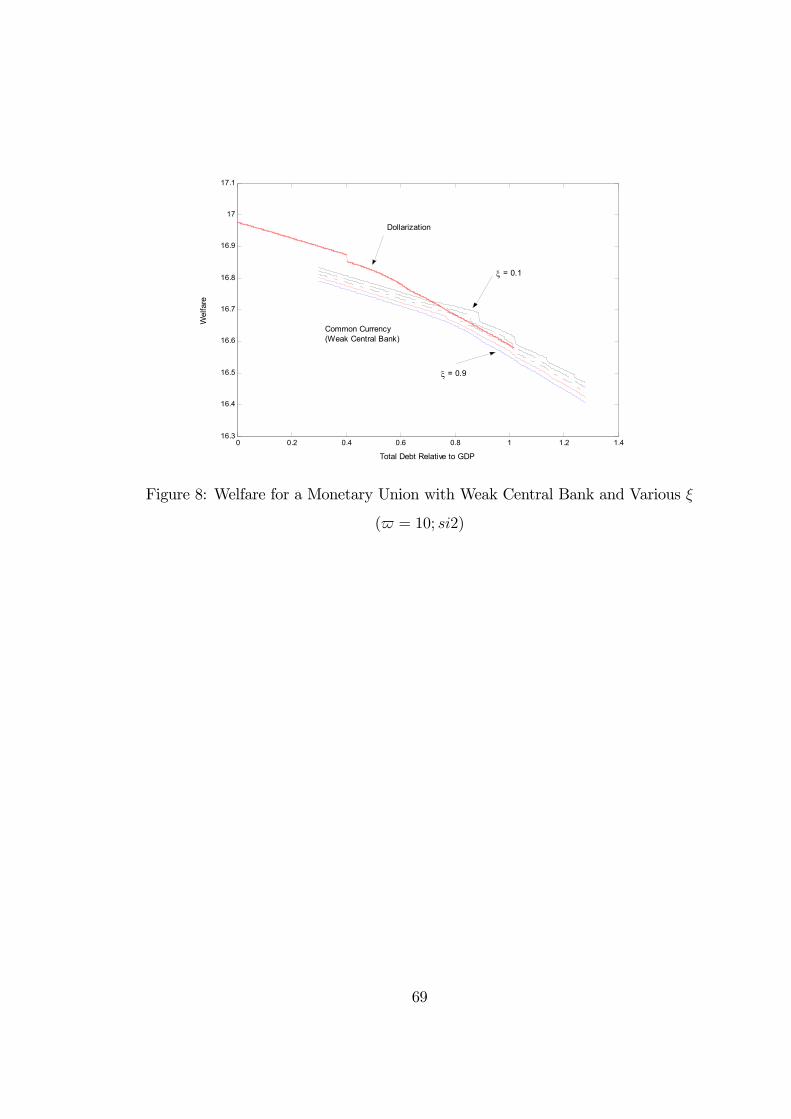
0 0.2 0.4 0.6 0.8 1 1.2 1.416.3

16.4

16.5

16.6

16.7

16.8

16.9

17

17.1


Wel

fare

ξ = 0.1

ξ = 0.9

Dollarization

Common Currency (Weak Central Bank)

Figure 8: Welfare for a Monetary Union with Weak Central Bank and Various ξ

( = 10; si2)

69

0 0.2 0.4 0.6 0.8 1 1.2 1.416.3

16.4

16.5

16.6

16.7

16.8

16.9

17

17.1


Wel

fare

Dollarization

Local Currency (Weak Central Bank)

Figure 9: Welfare for a Local Currency Regime with Weak central bank and

Various ξ

0 0.2 0.4 0.6 0.8 10

0.5

1LOCAL CURRENCY

New

Dol

lar D

ebt /

GD

P

45 degrees lineξ =0.1ξ =0.9

0 0.2 0.4 0.6 0.8 10

0.5

1DOLLAR

New

Dol

lar D

ebt

/ GD

P

0 0.2 0.4 0.6 0.8 10

0.5

1COMMON CURRENCY

New

Dol

lar D

ebt

/ GD

P

Dollar Debt / GDP

45 degrees lineξ =0.1ξ =0.9

Figure 10: Government Dollar Debt Policy Function

70

71

Banco Central do Brasil

Trabalhos para Discussão Os Trabalhos para Discussão podem ser acessados na internet, no formato PDF,

no endereço: http://www.bc.gov.br


Working Papers in PDF format can be downloaded from: http://www.bc.gov.br

1 Implementing Inflation Targeting in Brazil

Joel Bogdanski, Alexandre Antonio Tombini and Sérgio Ribeiro da Costa Werlang

July/2000

2 Política Monetária e Supervisão do Sistema Financeiro Nacional no Banco Central do Brasil Eduardo Lundberg Monetary Policy and Banking Supervision Functions on the Central Bank Eduardo Lundberg

Jul/2000

July/2000

3 Private Sector Participation: a Theoretical Justification of the Brazilian Position Sérgio Ribeiro da Costa Werlang

July/2000

4 An Information Theory Approach to the Aggregation of Log-Linear Models Pedro H. Albuquerque

July/2000

5 The Pass-Through from Depreciation to Inflation: a Panel Study Ilan Goldfajn and Sérgio Ribeiro da Costa Werlang

July/2000

6 Optimal Interest Rate Rules in Inflation Targeting Frameworks José Alvaro Rodrigues Neto, Fabio Araújo and Marta Baltar J. Moreira

July/2000

7 Leading Indicators of Inflation for Brazil Marcelle Chauvet

Set/2000

8 The Correlation Matrix of the Brazilian Central Bank’s Standard Model for Interest Rate Market Risk José Alvaro Rodrigues Neto

Set/2000

9 Estimating Exchange Market Pressure and Intervention Activity Emanuel-Werner Kohlscheen

Nov/2000

72

10 Análise do Financiamento Externo a uma Pequena Economia Aplicação da Teoria do Prêmio Monetário ao Caso Brasileiro: 1991–1998 Carlos Hamilton Vasconcelos Araújo e Renato Galvão Flôres Júnior

Mar/2001

11 A Note on the Efficient Estimation of Inflation in Brazil Michael F. Bryan and Stephen G. Cecchetti

Mar/2001

12 A Test of Competition in Brazilian Banking Márcio I. Nakane

Mar/2001

13 Modelos de Previsão de Insolvência Bancária no Brasil Marcio Magalhães Janot

Mar/2001

14 Evaluating Core Inflation Measures for Brazil Francisco Marcos Rodrigues Figueiredo

Mar/2001

15 Is It Worth Tracking Dollar/Real Implied Volatility? Sandro Canesso de Andrade and Benjamin Miranda Tabak

Mar/2001

16 Avaliação das Projeções do Modelo Estrutural do Banco Central do Brasil Para a Taxa de Variação do IPCA Sergio Afonso Lago Alves Evaluation of the Central Bank of Brazil Structural Model’s Inflation Forecasts in an Inflation Targeting Framework Sergio Afonso Lago Alves

Mar/2001

July/2001

17 Estimando o Produto Potencial Brasileiro: uma Abordagem de Função de Produção Tito Nícias Teixeira da Silva Filho Estimating Brazilian Potential Output: a Production Function Approach Tito Nícias Teixeira da Silva Filho

Abr/2001

Aug/2002

18 A Simple Model for Inflation Targeting in Brazil Paulo Springer de Freitas and Marcelo Kfoury Muinhos

Apr/2001

19 Uncovered Interest Parity with Fundamentals: a Brazilian Exchange Rate Forecast Model Marcelo Kfoury Muinhos, Paulo Springer de Freitas and Fabio Araújo

May/2001

20 Credit Channel without the LM Curve Victorio Y. T. Chu and Márcio I. Nakane

May/2001

21 Os Impactos Econômicos da CPMF: Teoria e Evidência Pedro H. Albuquerque

Jun/2001

22 Decentralized Portfolio Management Paulo Coutinho and Benjamin Miranda Tabak

June/2001

73

23 Os Efeitos da CPMF sobre a Intermediação Financeira Sérgio Mikio Koyama e Márcio I. Nakane

Jul/2001

24 Inflation Targeting in Brazil: Shocks, Backward-Looking Prices, and IMF Conditionality Joel Bogdanski, Paulo Springer de Freitas, Ilan Goldfajn and Alexandre Antonio Tombini

Aug/2001

25 Inflation Targeting in Brazil: Reviewing Two Years of Monetary Policy 1999/00 Pedro Fachada

Aug/2001

26 Inflation Targeting in an Open Financially Integrated Emerging Economy: the Case of Brazil Marcelo Kfoury Muinhos

Aug/2001

27

Complementaridade e Fungibilidade dos Fluxos de Capitais Internacionais Carlos Hamilton Vasconcelos Araújo e Renato Galvão Flôres Júnior

Set/2001

28

Regras Monetárias e Dinâmica Macroeconômica no Brasil: uma Abordagem de Expectativas Racionais Marco Antonio Bonomo e Ricardo D. Brito

Nov/2001

29 Using a Money Demand Model to Evaluate Monetary Policies in Brazil Pedro H. Albuquerque and Solange Gouvêa

Nov/2001

30 Testing the Expectations Hypothesis in the Brazilian Term Structure of Interest Rates Benjamin Miranda Tabak and Sandro Canesso de Andrade

Nov/2001

31 Algumas Considerações sobre a Sazonalidade no IPCA Francisco Marcos R. Figueiredo e Roberta Blass Staub

Nov/2001

32 Crises Cambiais e Ataques Especulativos no Brasil Mauro Costa Miranda

Nov/2001

33 Monetary Policy and Inflation in Brazil (1975-2000): a VAR Estimation André Minella

Nov/2001

34 Constrained Discretion and Collective Action Problems: Reflections on the Resolution of International Financial Crises Arminio Fraga and Daniel Luiz Gleizer

Nov/2001

35 Uma Definição Operacional de Estabilidade de Preços Tito Nícias Teixeira da Silva Filho

Dez/2001

36 Can Emerging Markets Float? Should They Inflation Target? Barry Eichengreen

Feb/2002

74

37 Monetary Policy in Brazil: Remarks on the Inflation Targeting Regime, Public Debt Management and Open Market Operations Luiz Fernando Figueiredo, Pedro Fachada and Sérgio Goldenstein

Mar/2002

38 Volatilidade Implícita e Antecipação de Eventos de Stress: um Teste para o Mercado Brasileiro Frederico Pechir Gomes

Mar/2002

39 Opções sobre Dólar Comercial e Expectativas a Respeito do Comportamento da Taxa de Câmbio Paulo Castor de Castro

Mar/2002

Date post:	07-Nov-2018
Category:	Documents
Upload:	truongbao
View:	221 times
Download:	0 times

Working Paper Series - Banco Central do Brasil · Working Paper Series ISSN 1518-3548 Speculative...

Documents