Congestion pricing can optimize traffic in two ways; by adjusting the total traffic volume so that the
marginal social cost of trips equal their marginal social benefit, and by adjusting the scheduling of trips to achieve
the minimum social cost. The standard congestion pricing model includes the first but not the second objective,
while the bottleneck model includes both. The standard model applies the theory of the firm to the production of
highway trips by interpreting the average cost curve as the individual travel time function and the marginal cost
curve as the social travel time function. The intersection of the average cost and demand curves determines the
untolled equilibrium that involves too many trips. The vertical difference between individual and social travel times
is the external time an individual trip imposes on other travelers. Imposing a toll equal to this difference implements
an optimal decentralized equilibrium, with marginal social costs (supply) equal to benefits (demand), by “tolling
off” travelers whose willingness to pay is below their social cost. The standard model is essentially static, with travel
time being a function of current traffic volume alone. Delays do not carry over from one period to the next.
Travelers do not optimize the choice of when to travel. There is no cost of schedule delay, i.e., deviating from a
preferred schedule time. Applying the standard model over time requires dividing time into multiple static periods
(possibly with cross elasticities of demand between periods). Dividing time into shorter time periods captures more
of the variation in demand, and allows for exogenous demand peaks, but limits the effect of recent traffic levels on
current congestion.
The bottleneck model has several significant advantages over the standard model, particularly as applied to
airports. First, it explicitly models the optimal choice of when to travel by trading off schedule delays against
queuing delays and any congestion tolls. Second, it has a queuing system that depends on the current state (length)
of the queue as well as the current traffic rate. The state dependent queuing system accounts for the entire history of
traffic rates and carries accumulated queues forward in time. Third, the scheduling of traffic and evolution of queues
occur in continuous time. Fourth, the bottleneck model provides a richer environment for analyzing interactions
between dominant and fringe airlines than the standard model because it models the dynamics of airport queuing
delay and the optimal timing of aircraft arrivals and departures that adjust in response to congestion levels and tolls.
This paper extends the deterministic bottleneck model to include a dominant airline that determines the optimal level
of internalizing or atomistic behavior by choosing of the number and timing of its aircraft operations. It develops a
general step-tolling model for which the no-toll and continuously-varying toll equilibria are the limiting cases as the
number of tolling steps goes from zero to infinity. This unified model of tolling demonstrates how the dominant-
fringe equilibria interact with the tolling structures.
Following the literature review, the theory section presents the unified model of bottleneck tolling
equilibria. Next, the paper demonstrates six propositions concerning airline behavior in untolled and tolled
equilibria, under the alternative assumptions that dominant and fringe airlines have homogenous operating time
preferences and valuations of time, homogenous time preferences and heterogeneous time valuations, and
heterogeneous preferences and valuations. The propositions specify how these assumptions affect whether the
dominant airline internalizes or behaves atomistically and how the tolls interact with airline behavior in establishing
an optimal equilibrium. A brief preview of these propositions is as follows: 1) When dominant and fringe aircraft
3
have homogeneous time values and preferences, the dominant airline goes from fully internalizing to fully atomistic
behavior as fringe demand elasticity goes from perfectly inelastic to elastic. 2) In the same homogeneous case,
dominant and fringe tolls vary by a constant amount which approaches zero as dominant aircraft approach fully
atomistic behavior, or as step tolls approach continuous variation. 3) Dominant aircraft with higher values of
schedule delay time provide an independent rationale for atomistic behavior. 4) Atomistic step tolls produce the
same aggregate traffic and queuing patters with either homogeneous or heterogeneous time values. Atomistic tolls
do not cause the dominant airline to double internalize delays. 5) Fringe aircraft with dispersed operating time
preferences increase the likelihood of atomistic behavior by the dominant airline. 6) Tolling is qualitatively similar
but not as analytically straightforward when fringe aircraft have heterogeneous time preferences. A final proposition
and theory section demonstrate the conditions under which an optimally-tolled airport with dominant and fringe
airlines is self financing. The paper concludes with a discussion of the model’s policy implications.
Review of the literature
William Vickrey (1969) developed the bottleneck model to provide a dynamic model of congestion with
travelers that adjust their times of travel optimally to minimize the sum of their trip duration and schedule delay
costs. Vickrey's congestion technology is a deterministic queue that develops at a highway bottleneck preventing
travelers from all arriving at their destinations at their most preferred times. The queue length depends on the entire
traffic pattern starting from the most recent time it was empty and affects future travel delay until the queue is empty
again. The no-toll equilibrium traffic and queuing patterns adjust endogenously over time so that identical travelers
have the same total costs of queuing and early or late arrival times. The optimal tolls adjust continuously throughout
the peak period to shift traffic and reduce queuing delay. With deterministic queuing, the toll completely replaces the
queue and converts all queuing costs into revenues. The model’s improvements over the standard model include:
dynamic treatment of congestion, explicit modeling of travelers' choices of travel times, endogenous peaking of
traffic and delay, and inclusion of schedule delays associated with travel time decisions.
Unfortunately, the economics literature largely ignored the bottleneck model until the late 1980's and even
now the standard model still appears to be the preferred framework for modeling congestion. Richard Arnott, André
de Palma, and Robin Linsey (1990) revived the bottleneck model in the economics literature by formalizing it,
extending it to include a coarse (single-step) toll, and determining the optimal capacity. Arnott, et al., (1993)
subsequently determined the optimal uniform, coarse, and continuous tolls with elastic demand. They demonstrate
that applying the standard model to subintervals of the peak period is conceptually unsound, but that the standard
model can represent a “semi-reduced form” of the entire peak period. They also show that efficiency gains are
substantially greater when accounting for endogenously chosen travel times than those estimated with the standard
model. They demonstrate that the self financing properties of Herbert Mohring and Mitchell Harwitz (1962) and
Robert Strotz (1965) apply to the bottleneck model whenever the pricing regime optimizes traffic levels under
whatever constraints on the form of pricing that the airport faces. Ralph Braid independently extends the bottleneck
model to cover elastic demand. Arnott, et al., (1989) and Yuval Cohen (1987) extend the bottleneck model to
heterogeneous travelers.
4
Daniel (1991) develops a bottleneck model with deterministic congestion that is non-linear in traffic rates
and applies the model to a stylized hub-and-spoke airline network. Daniel (1995) develops a bottleneck model with
stochastic queuing and includes Nash and Stackelberg dominant airlines with atomistic or non-atomistic traffic. He
implements the stochastic bottleneck model empirically using tower log data from Minneapolis-St. Paul airport and
performs specification tests that suggest Northwest Airlines does not internalize its self-imposed delays. In
particular, Northwest flights apparently do not adjust their operating times to account for delays they impose on
other Northwest flights. Daniel (2001) extends the stochastic bottleneck model to include elastic demand,
heterogeneous aircraft costs, and fringe aircraft with uniformly distributed preferred operating times.
Brueckner (2002) develops a congestion pricing model with a dominant airline and a competitive fringe
using the standard congestion technology in which the dominant airline internalizes its self-imposed delays so that
its optimal congestion fee is inversely proportional to its market share. Brueckner also uses on-time performance
data aggregated by airport per annum to show that more concentrated airports have less delay. Mayer and Sinai
(2003) perform an extensive empirical study of the concentration-delay relationship using data on excess flight
times over minimum flight times by city-pair routes. They use dichotomous variables to control for level of hubbing
activity by airport. They find a statistically significant, inverse relationship between airport concentration and excess
flight time, which they interpret as evidence of internalization by the dominant airlines. They also find a much
stronger direct relationship between hubbing activity and delays.
Daniel and Harback (2008) applies Daniel's (1995) specification test of internalization verses non-
internalization to twenty-seven major hub airports, finding that dominant airline flight schedules are more consistent
with minimizing individual aircraft costs rather than joint costs. They argue that in the stochastic bottleneck model,
the atomistic fringe's adjustment of its flight times in response to peak spreading by the dominant airline (in an
attempt to internalize self-imposed delays) offsets any reduction in peak traffic. The internalizing dominant airline
realizes more schedule and queuing delay than it expects under the Nash assumption that fringe schedules do not
change. Knowing this, a Stackelberg dominant airline behaves atomistically. Brueckner and van Dender (2008) seek
to unify the internalization versus non-internalization debate using a simple transparent model with two periods and
the standard congestion technology. They criticize the stochastic bottleneck model of Daniel (1995) and Daniel and
Harback (2008) as opaque because the stochastic queuing system prevents closed-form solution of the model.
Brueckner and van Dender obtain either internalization or non-internalization as the dominant airline's optimal
solution depending on the fringes’ demand elasticity for aircraft operations during the congested period. Daniel
(2009b) applies a deterministic bottleneck model with dominant and fringe traffic to airport slot constraints. That
paper develops a similar unconstrained equilibrium as developed here, but addresses quantity restrictions rather than
congestion pricing.
This paper parallels that of Brueckner and van Dender (2008) by using a deterministic bottleneck model
with explicit closed form solutions to show the conditions under which either internalization or non-internalization
is an optimal strategy for the dominant airline. Although the deterministic bottleneck model is more complicated
5
than a two-period model with the standard congestion technology, it provides a richer environment for modeling the
effects of congestion and pricing on aircraft scheduling. The state-dependent queuing system captures the dynamic
nature of congestion. The model also includes schedule delay among the private and social costs. This paper
contributes to the existing literature by developing three specifications of the bottleneck model in which a dominant
firm may internalize or behave atomistically based on elastic demand of the fringe aircraft, higher schedule delay
costs of the dominant airline, or more dispersed operating-time preferences of fringe aircraft. The dominant airline
may adopt atomistic, internalizing, or mixed behavior in each specification depending on the parameterization of
time values and demand elasticities. In all cases of fully atomistic behavior and for all continuous tolls, the step
tolling rules for the dominant and fringe aircraft are similar. The internalizing and mixed cases generally require an
additional uniform tool that differentiates between dominant and fringe aircraft, but not simply on the basis of traffic
shares. The paper also determines the optimal airport capacities and demonstrates that tolling revenues equal
optimal capacity costs under constant returns to airport capacity construction when there are dominant and fringe
operations. Unlike Daniel’s (1995) stochastic bottleneck model, the deterministic version produced here has closed
form solutions for all specifications.
The model
The deterministic bottleneck model is a structural model that explicitly treats the dynamic nature of airport
congestion and scheduling decisions of aircraft operators. In particular, it models changes in congestion over time
depending on the current arrival rate and the current state (length) of the queue, and it models the optimal scheduling
of traffic to minimize the costs of schedule delay and queuing delay. This paper extends the atomistic bottleneck
model with deterministic queues to explicitly solve the problem of a dominant airline that jointly schedules large
groups of aircraft, and an atomistic fringe that schedules each aircraft independently of the others. Because of the
model’s dynamic congestion technology and optimal timing of traffic, it offers the possibility of reducing congestion
by spreading peak traffic. When a dominant airline internalizes its self-imposed delays it does so primarily by
spreading its traffic to even out the arrival rates rather than by reducing the number of flights.1 Several plausible
scenarios lead to different behavior by dominant airlines. These include homogenous dominant and fringe aircraft
with elastic demand, dominant aircraft that have higher schedule delay values than the atomistic fringe, and
atomistic fringe aircraft that have uniformly distributed operating times. The scheduling behavior and equilibrium
travel costs differ across these scenarios in ways that affect the structure of efficient tolls. The multi-step tolling
model developed below includes the uniform and coarse tolls of Arnott, et al. as special cases. Vickrey’s
continuously varying toll is the limiting case as the number of different steps in the toll structure increases. This
unified treatment of the tolling structures covers all the relevant cases of time dependant tolling.
Review of the bottleneck framework
Consider a dominant airline providing hub-and-spoke service during a particular busy period with demand
for landings or takeoffs (operations) given by d=dpd], where pd is the full price of a dominant aircraft operation that
1 Peak spreading can reduce the full price of operating so much that the dominant airline actually increases its number of aircraft
relative to the atomistic equilibrium.
6
is determined below. As the next subsection will justify, x of these dominant aircraft operate atomistically during the
peak and d-x operate during the service intervals before and after the peak without creating any queuing delay. There
is a group of fringe airlines, each of which operates a single aircraft during the peak2. The demand for operations by
fringe aircraft is f=fpf] where pf is the full price of a fringe operation. The dominant airline needs to schedule its
aircraft around a passenger interchange period to facilitate connecting service. Assume initially that the fringe also
prefers to schedule its aircraft at these times, because they are popular travel times for passengers. For the rest of this
sub-section, it is not necessary to distinguish between the f fringe and x dominant aircraft. Let m=f+x be the total
number of operations during the atomistic peak. Let tL* and tT
* be the most preferred times near the beginning and
ending of the interchange period. Runway capacity limits the landing and takeoff rates to s aircraft per minute. Air
traffic control alternates landing and takeoffs in such a way that they do not impose delays on each other.3 Let rL[t]
and rT[t] be the rate of aircraft joining the landing and takeoff queues at time t. Separate deterministic queues for
landings and takeoffs develop at the runway bottlenecks from time tab , when the queue is empty, according to the
equation:
(1) .
Assume initially that all aircraft have identical time costs. Aircraft operate before or after their preferred
times at cost and dollars per minute. Time spent in the queue costs dollarsper minute. The subscripts L or T
that differentiate landing or takeoffs are suppressed because the model is the same in either case aside from possibly
different time values. Private landing or takeoff costs are:
(2) .
In a no-fee atomistic bottleneck (Nash) equilibrium, fringe traffic adjusts to maintain constant costs C.[t]=C* across
all times in which fringe aircraft operate. Solve for r[t] separately when t is early, t ≤ t.*- q.(t)/s, or late, t > t.
*- q.(t)/s,
by substituting (1) into (2) and differentiating with respect to t while imposing the constant cost condition. This
gives the aggregate traffic rates during fringe operating times:
(3)
Equations (1)-(3) represent the essential structure of the deterministic bottleneck model that Vickrey (1969) and
Arnott, et al. (1990) developed. We now develop a unified model of multiple-step tolling.
2 The “peak” refers to the period of time during which the airport is congested, i.e., there is a queue. The “busy” period refers to
the period of time during which the arrival rate is positive. The busy period includes the atomistic peak and the internalizing
dominant operations.
3This is approximately true of actual airports operating under balanced traffic (landing and takeoff) conditions. The author's
observations of traffic counts indicate that somewhat higher rates of takeoff are possible when there are no landings, but that
no additional landings are possible when there are no takeoffs.
7
The unified bottleneck tolling model
To solve the multiple-step tolling problem, the airport authority takes the number of toll periods
exogenously and chooses a toll for each period and the beginning and ending times, t1 and t2, of the central toll
period. The increments in toll levels determine the duration of the remaining toll periods. In cases for which the
value of late time exceeds that of queuing time (, the airport authority also chooses a time t that shifts the entire
busy period slightly later to trade off overall schedule delay against queuing delay.4 For airports, empirical estimates
of the queuing time values generally exceed the late time value, so there is no such shifting. For the sake of
generality, the optimization program includes t as a choice variable with the understanding that when the value of
queuing time exceeds that of late time, its first order condition should be replaced by the constraint t =0.
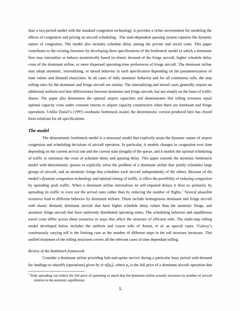
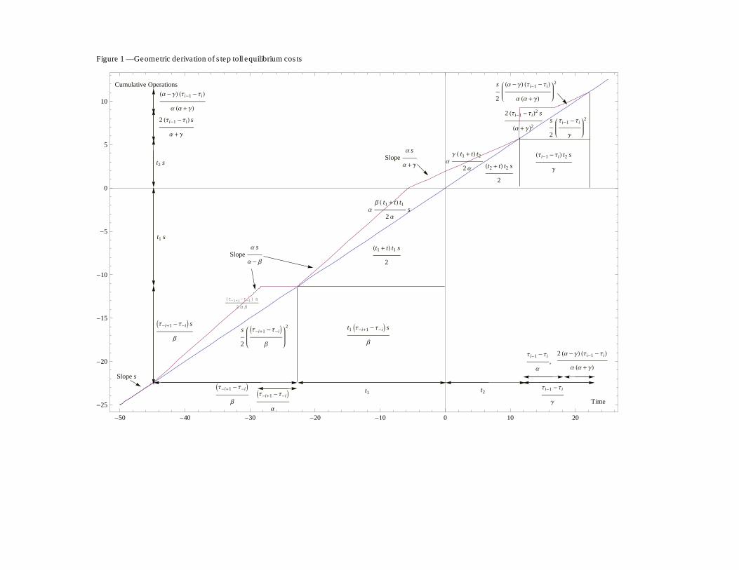
The simplest way to derive the multiple-step toll is by reference to Figure 1 that shows the central peak and
some surrounding toll periods. The cumulative service function is a straight line with slope s equal to the service
rate. The most preferred operating time is normalized to zero. To derive the total social cost of all the operations, it
is necessary to determine the areas of the labeled triangles and rectangles. Those above the cumulative service
function have area equal to the total queuing time. Those below and to the left of t* have area equal to total early
time, and those below and to right have area equal to total late time. The beginning and ending times of the central
peak are choice variables, with t shifting the entire peak horizontally relative to t*. This shift enables the airport
authority to start the peak sooner or later relative to t* so that the fraction of early to late aircraft varies, which is not
possible by varying only t1 and t2. To accomplish this, add or subtract t to t1 and t2 in the horizontal (time)
dimension, but not the vertical (aircraft) dimension. Using the traffic rates in Equation (3) and simple geometry, the
total early time delay in the central peak is (t1+t) t1s/2 and the total late time delay is (t2-t) t2s/2. Queuing time for
the aircraft operating early is (t1+t)t1s/(2) and (t2-t)t2s/(2) for those operating late.
In the early toll periods immediately to the left of the central peak, the horizontal line segment represents
the length of time before imposition of the central peak toll, 0, during which no new arrivals at the queue occur
because the toll temporarily raises the full price of operating above the equilibrium cost. The queuing time cost must
diminish to equate the full cost of the last aircraft in the toll period with the first aircraft in the next, so the line
segment has length (0--1)/where -1 is the toll in period just before the central peakSimilar logic requires the
first and last aircraft in this toll period have the same full price so that its length is (0--1)/Simple geometry
determines the queuing delay to be (0--1)2s/(2and schedule delay to be 2(t1+t)(0--1s(0--1)
2s/(2
4 Shifting the entire busy period earlier (later) decreases (increases) the amount of queuing delay experienced by late aircraft, but
decreases (increases) their late time and increases (decreases) the early time of early aircraft. This adjustment cannot occur in
the untolled, single tolled, or fine-tolled cases, or when (, because the schedule delay of the first and last vehicle must be
equal. In the multi-step tolling cases when (t shifts the busy period later. As shown below, the last group of flights
operates all at once and is served in random order. These aircraft have expected total cost equal to the equilibrium level, but
the actual costs of the last several aircraft are higher than the equilibrium level. The late aircraft do not deviate from the
equilibrium because their expected cost is identical to all the other aircraft, and earlier aircraft do not deviated because
following the late aircraft would increase their costs. When when (, t cannot shift the busy period forward because this
would raise early aircraft costs and lower late aircraft. The first several aircraft would deviate to follow the last aircraft and
reduce their costs until the constant cost condition held. See also, Arnott, et al., (1993) footnote 8.
8
The vertical line immediately following the central peak represents a mass of aircraft that depart
immediately after the central peak toll is lifted. It must increase (expected) queuing and late time costs enough that
the last aircraft in the central peak has the same cost as the (expected) cost of all the aircraft in the next toll period.
Assuming random admission to the queue, this mass arrival must include 2(0-1)s /(2(aircraft where 1 is the
toll in the toll window immediately following the central peak. If the value of queuing time exceeds that of late time
(then the delay costs decrease rapidly enough to reach the equilibrium level before the queue empties. In this
case, traffic resumes after (0-1)/minutes, at the late rate, sand the queue diminishes gradually until it
empties exactly at the end of the tolling period, (0-1)/minutes after it started. The total queuing time is
4(0-1)2s/(2(+(0-1))
2s and the total late time is (0-1t2s/+(0-1)
2s/(2. When
(then there are no operations between the mass at the beginning of the toll period and a similar mass at the
beginning of the next toll period. The queuing costs are just 4(0-1)2s/(2( and the schedule delay costs are
2(t2-t)(0-1s/(2()+4(0-1)2s/(2( The delay times in the additional tolling periods on either side of the
central peak vary only with their toll increments and their distance from t*. The derivation of time costs for
additional pairs of tolling periods is similar.
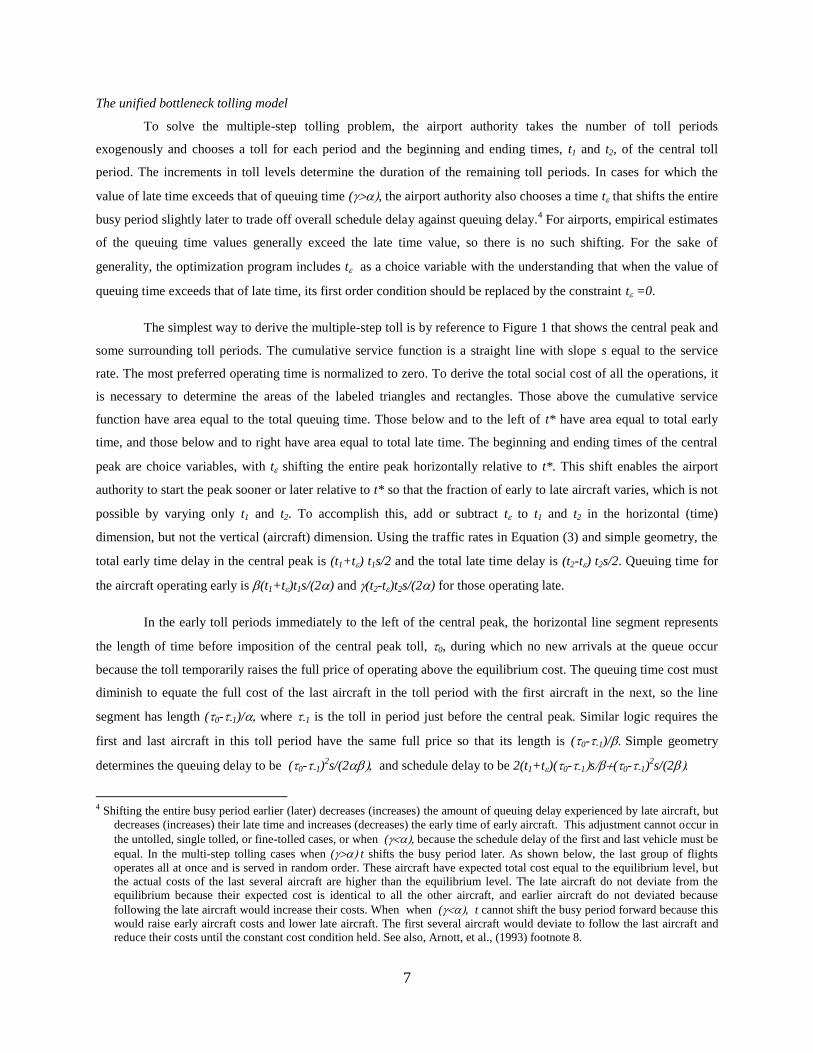
The airport authority’s problem is to choose t, t1, t2, -y, …, z to minimize the total cost of aircraft in a step
toll regime with a given number of early and late tolling periods, y and z, subject to the constraint that all aircraft are
served. Its objective function is:
(4)
,
subject to
,
, and
. .
The general solution in terms of the number of steps, y and z, is obtained by solving (4) for specific
numbers of steps, “guessing” the general the solutions, and verifying that the general solutions satisfy the first and
second order sufficient conditions of (4). Let r[-x, y] denotes a particular step in the tolling structure, including the
9
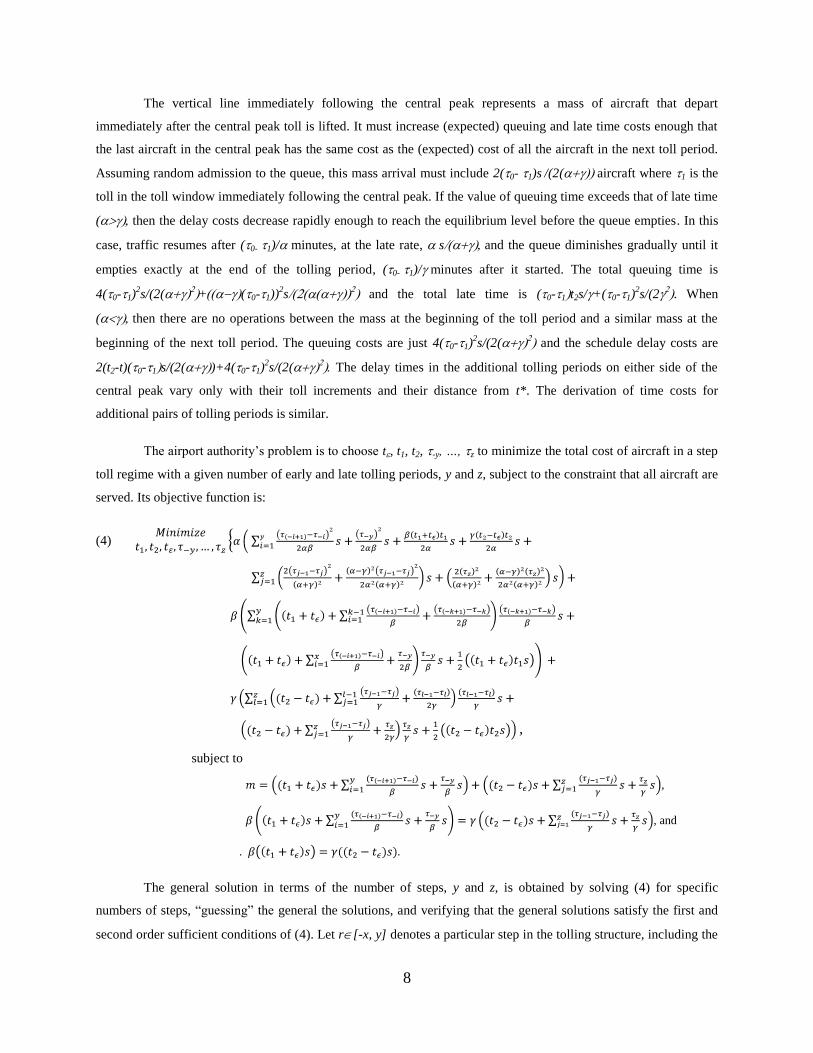
zero price step. Define the expressions, , and to express the general solution for the multiple-step toll
structure when as:
(5)
,
,
+
;
, where ;
; ; and .
The minimized value of the total cost function is:
(6) , where .
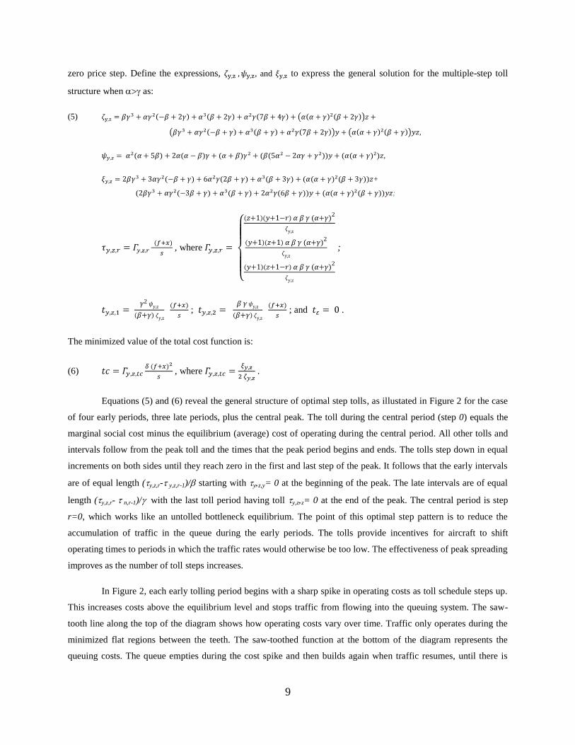
Equations (5) and (6) reveal the general structure of optimal step tolls, as illustated in Figure 2 for the case
of four early periods, three late periods, plus the central peak. The toll during the central period (step 0) equals the
marginal social cost minus the equilibrium (average) cost of operating during the central period. All other tolls and
intervals follow from the peak toll and the times that the peak period begins and ends. The tolls step down in equal
increments on both sides until they reach zero in the first and last step of the peak. It follows that the early intervals
are of equal length (y,z,r- y,z,r-1)/ starting with yz,y= 0 at the beginning of the peak. The late intervals are of equal
length (y,z,r- n,r-1)/ with the last toll period having toll y,zz= 0 at the end of the peak. The central period is step
r=0, which works like an untolled bottleneck equilibrium. The point of this optimal step pattern is to reduce the
accumulation of traffic in the queue during the early periods. The tolls provide incentives for aircraft to shift
operating times to periods in which the traffic rates would otherwise be too low. The effectiveness of peak spreading
improves as the number of toll steps increases.
In Figure 2, each early tolling period begins with a sharp spike in operating costs as toll schedule steps up.
This increases costs above the equilibrium level and stops traffic from flowing into the queuing system. The saw-
tooth line along the top of the diagram shows how operating costs vary over time. Traffic only operates during the
minimized flat regions between the teeth. The saw-toothed function at the bottom of the diagram represents the
queuing costs. The queue empties during the cost spike and then builds again when traffic resumes, until there is
10
another toll increment. In the late periods there is a rush to join the queue each time the toll schedule steps down.
Queuing costs must jump by twice the toll increment so that the average increase just offsets the reduction in the
tolls. This causes another cost spike that stops the traffic flow until queue diminishes sufficiently to reestablish the
equilibrium costs. When there are no tolls, the queuing costs continue to build throughout the early period,
eventually peaking at the equilibrium cost level for the aircraft operating precisely at the most preferred time.
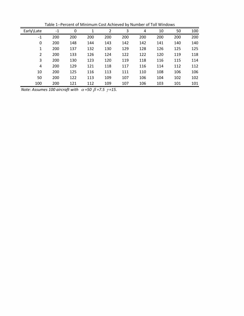
Step tolling recovers some of the deadweight loss from queuing in the form of airport revenues. The
amount of the efficiency gain depends on the value of in Equation (6) that is largely determined by the number
of tolling periods. Table 1 shows how the efficiency of the step toll system varies with the number of early and late
steps. The table uses cost parameter, ,,and , that are typical of those Daniel and Harback (2009a) estimate for
major hub airports in the US, but the overall efficiency results in the table are not particularly sensitive to variations
in the cost parameter. The parametersand affect the relative advantage of early versus late tolling periods.
Efficiency improves rapidly as the number of steps increases; one step on each side of central period recovers half
the efficiency loss from congestion, while five early and three late steps plus the central period recovers eighty
percent of the loss.
When the numbers of early and late steps, y and z, go to minus one in the limit, there is only a central
period with one toll level. This specification of the model gives the no toll or uniform toll equilibria, which have the
same cost functions because zero or one (uniform) toll level has no effect on traffic schedules. The value of in
these cases is one. As the values of y and z go to infinity, approaches one-half. The general solution for any
atomistic step-toll equilibrium has the total (social) congestion given in Equation (6) as m2/s. The price of a
single landing or take off is the average congestion cost (m)/s. The marginal social cost of a landing or takeoff
is 2 m/s or twice the full price of the operation. Using a superscript e to denote an unpriced equilibrium, the
atomistic costs are as follows:
(7) and where
Equations (7) give the atomistic solution in the unpriced bottleneck equilibrium as specified by Vickrey (1969) and
Arnott, et al. (1990, 1993) as special cases. Arnott, et al. (1993) notes that even though there is a dynamic structural
model underlying Equations (7), all travelers face a common full price (ATC) so that the entire peak period is
represented by a trip supply function, p=m/s. We now extend the model to determine the dominant and fringe
equilibrium traffic patterns and demand.
Dominant and fringe airlines with homogeneous time values and preferences
Proposition 1: When dominant and fringe airlines have identical time values and operating-time
preferences, the unpriced equilibrium has an atomistic bottleneck equilibrium surrounding t* that
includes all of the fringe aircraft and a fraction of the dominant aircraft that varies from zero (the
perfectly inelastic case) to one (if fringe demand is sufficiently elastic). The dominant airline
internalizes the self-imposed delays of its remaining aircraft by scheduling them to operate before
11
and after the atomistic peak at exactly the rate of service. These internalizing dominant aircraft do
not create or experience any queuing delay.
Recall the distinction between dominant and fringe demand, with d and f denoting the total number of
operations, and x denoting the number of dominant operations scheduled during the atomistic peak. Equation (3)
now gives the aggregate traffic rates that are necessary to satisfy the equilibrium condition in Equation (2). The
dominant airline has no incentive to exceed these rates during the atomistic peak because doing so would increase its
queuing delay without reducing its schedule delay. The best (scheduling) responses of the atomistic fringe as
functions of the dominant airline’s arrival rates are:
(8)
.
The rates for C[t]>C* and C[t]<C* represent corner solutions in which the fringe ceases operations when the cost is
above the equilibrium level, or it instantaneously schedules sufficient operations to cause the queue to satisfy the
equilibrium condition when cost would otherwise be below the equilibrium level.
In the no-toll case where =1, the full price for a fringe aircraft operation is f+x)s. To obtain explicit
solutions for the fringe demand, it is useful to assume linear demand. Let the supply and demand functions be given
in Equation (9), and substitute the supply price into the demand function to solve for the optimal number of the
fringe aircraft, f, as a function of the number of dominant aircraft scheduled during the atomistic peak, x[d].
(9) , , and .
Now consider the dominant airline’s problem of scheduling aircraft before or after the atomistic peak.
These aircraft cannot obtain service more rapidly than the service rate s, and will have no queue if they operate at or
below rate s. It follows that s is the least costly operating rate. Applying the second constraint of (4) to determine the
operating times of the first and last dominant aircraft, tdb and tde gives the dominant airline’s traffic pattern for
aircraft not scheduled during the atomistic peak:
(10) where and .
There are /() (d-x) early aircraft that experience early time of (d+x+2f)/(()2s) and (d-x) /() late
aircraft that experience late time of (d+x+2f)/(()2s). Multiplying the numbers of aircraft by their time values
and average delay times gives the total cost of the internalizing dominant aircraft. Adding the total cost of the
dominant aircraft in the atomistic peak and substituting the fringe demand gives the dominant airline’s objective
12
function. The dominant airline’s problem and solution choosing the number of aircraft to schedule during the
atomistic peak are:
(11) , s.t. , and .
Let s+) be the fraction of dominant aircraft scheduled during the atomistic peak. Substituting d for x[d]
in the dominant airline’s average cost and simplifying yields the full price, or airport supply function, for a dominant
aircraft operation in the untolled equilibrium. Let the supply and demand functions for dominant airline operations
be:
(12) and
The number of aircraft in the untolled equilibrium simultaneously satisfies the supply and demand functions as
given in Equations (9) and (12). Let , and be the number of aircraft in the untolled equilibrium. Let and
be the equilibrium full prices of fringe and dominant aircraft. The reduced form solutions for equilibrium prices and
quantities are:
(13) ; ;
; and ,
where .
When =0, this is the fully internalizing solution; when 0 <<1 it is the mixed solution; and as approaches one, it
approaches the fully atomistic solution. This and Equation (10) complete the demonstration of Proposition 1.
To understand the intuition behind this result, suppose that fringe demand were inelastic but there were
some dominant aircraft in the atomistic peak. All of the periods during the atomistic peak have the same equilibrium
cost, so the dominant airline could always reschedule any of its aircraft from the atomistic peak to the edges of the
peak without increasing their cost. Atomistic aircraft would shift to fill the gaps in traffic left by the dominant
aircraft. The dominant airline would set the traffic rates of the rescheduled aircraft equal to the service rate so that
they would not impose delays on one another. The length of the atomistic peak would decrease by one service
period for each rescheduled dominant aircraft. The equilibrium cost in the atomistic peak would decrease to equal
that of the dominant aircraft at the edge of the peak. This process would continue until no dominant aircraft
remained in the atomistic peak.
With elastic demand, moving dominant aircraft out of the atomistic peak reduces the average cost (full
price) of atomistic operations at the rate of /s per aircraft, which induces additional fringe aircraft to enter the peak,
13
driving the cost up. As new fringe aircraft enter, the peak period re-expands, pushing the internalizing dominant
aircraft away from their preferred operating time. If new fringe entry only partially offsets the cost reduction, then
dominant aircraft remaining in the atomistic peak benefit from internalizing. The dominant airline balances the
reduction in cost for its atomistic aircraft against the increase in cost of its internalizing aircraft. If fringe demand is
sufficiently elastic, then x approaches d; i.e., the dominant airline leaves all its aircraft in the atomistic peak to
preempt entry by the fringe.
The tolling equilibria with homogeneous time values and preferences
Proposition 2: When dominant and fringe airlines have the same time values and preferences,
imposing the same atomistic step-toll schedule achieves the constrained-optimal scheduling of
aircraft. Different uniform tolls are necessary to account for the effects of internalizing dominant
aircraft that operate outside the peak. These uniform tolls optimize the number of dominant and
fringe operations. As the dominant airline schedules more aircraft during the atomistic peak, the
optimal tolls for both dominant and fringe aircraft approach those of the undifferentiated equilibria
with fully homogeneous atomistic aircraft. Continuously varying (fine) tolls fully internalize all
delays and are identical in cases with homogeneous dominant and fringe aircraft. Tolling
internalizing-dominant aircraft does not cause them to double internalize their delays.
The basic principles of tolling require that every aircraft face a full price of operating equal to its full social
costs. This assures the correct number and optimal scheduling of operations. The multiple-step tolling model shows
how to toll aircraft operating in the atomistic peak, but it does not directly cover the external costs these aircraft
impose on off-peak aircraft. An additional uniform toll is needed to cover their effect on the internalizing dominant
aircraft. This toll affects the number but not the scheduling of atomistic aircraft. Recall the total, marginal, and
average costs for the atomistic peak from Equation (7). The airport authority’s problem is to set the atomistic
aircrafts’ full prices equal to their marginal social costs by setting the uniform toll equal to the difference between
their marginal social cost and average (private) cost. Here the average cost ( of the atomistic aircraft is the
equilibrium social cost of operations during the atomistic peak, including the step tolls. The additional uniform
toll ) is the additional delay imposed on the internalizing dominant aircraft. Substituting the fringe full price in
its demand function gives the fringe’s optimal demand under the step toll as a function of the dominant airline’s
demand and number of aircraft scheduled during the atomistic peak:
(14) ,
, , and .
The dominant airline chooses the number of aircraft to schedule during the atomistic peak to minimize the
sum of its internalizing and atomistic aircraft costs. The toll accounts for the change in social costs as the number of
dominant aircraft in the atomistic peak changes. The dominant airline’s problem and solution are:
(15) .
14
The airport authority sets the dominant aircraft full prices equal to their marginal social costs by setting the tolls
equal to the difference between their marginal social costs and average (private) cost. The full prices, average costs,
and uniform tolls, are:
(16) ; ; and .
; ; and .
The dominant toll includes the producer surplus from its internalizing aircraft that it retained in the untolled
equilibrium, plus the atomistic fee on its aircraft in the atomistic peak. This is importantly different from the
dominant toll in the standard model which is the atomistic toll times one minus by the dominant airline’s share of
traffic. When approaches d, the dominant airline behaves more atomistically and its full price approaches that
of the fringe aircraft. As approaches zero the dominant airline can self internalize without facing much
additional fringe entry. It imposes less delay on the fringe and hence has both lower marginal and average costs.
The number of aircraft in the tolled equilibrium simultaneously satisfies the demand functions as given in
Equations (9) and (12) and the supply functions as given in Equations (16). Let , and be the number of aircraft
in the step-tolled equilibrium. Let and be the equilibrium full prices of fringe and dominant aircraft. The
reduced form solutions for equilibrium prices and quantities are:
(17) ; ;
; .
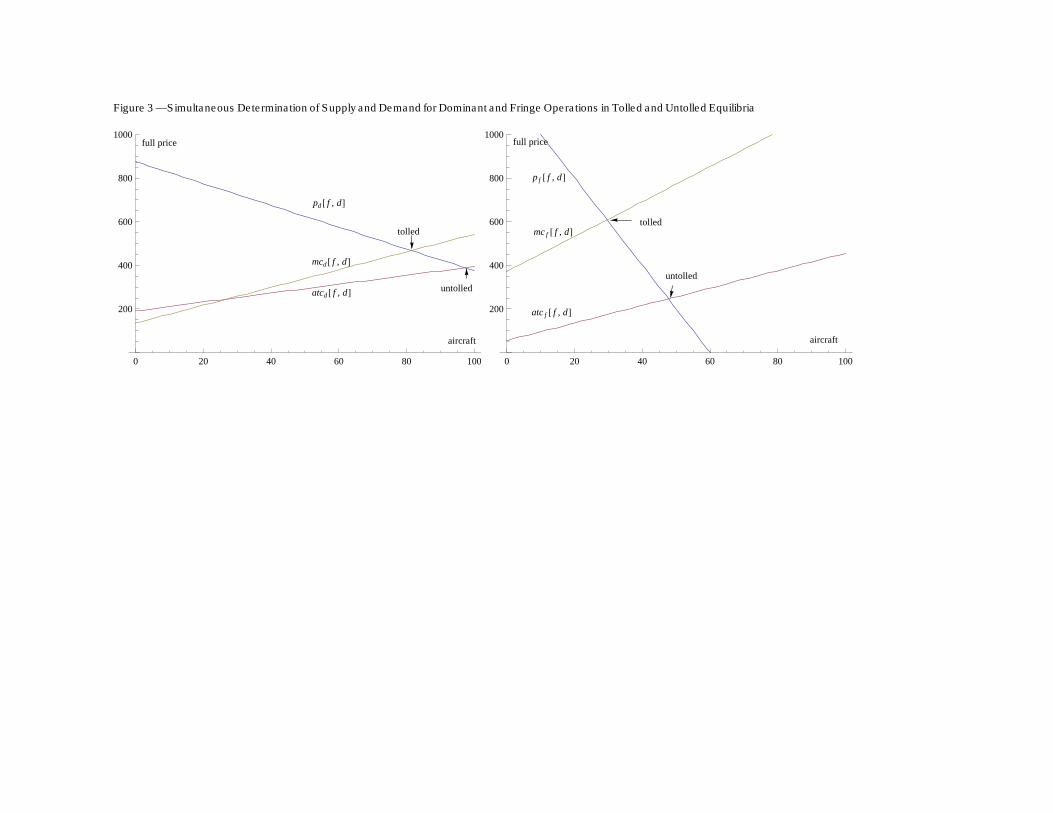
The top panels of Figure 3 illustrate the untolled and step tolled equilibria for homogenous fringe and
dominant and aircraft respectively. As Arnott, et al. (1993) observed, the reduced form of the bottleneck equilibrium
appears similar to the standard model applied to the entire peak period, but it has a structural model of airport supply
based on the underlying congestion technology and optimal aircraft scheduling. Figure 3 illustrates that
determination of equilibrium full prices and quantities reduces to standard supply and demand diagrams, with the
bottleneck model determining the shape of airport supply functions. A critical difference between previous atomistic
bottleneck models and the dominant-fringe specification developed here is that the supply functions must account
for the interaction between dominant and fringe operations. Each type of operation imposes a negative externality in
production on the other. The supply curves depicted in the graph are actually projections of supply surfaces in fd
space that account for the number of both types of operations. The tolled and untolled supply curves are projections
of these surfaces holding the other output constant at the corresponding tolled or untolled equilibrium level. The
position of the untolled supply surface at the tolled equilibrium output levels is different from its position at the
untolled equilibrium level, so the toll is not the vertical difference between the depicted supply projections—as it
15
would be in both the standard model and the atomistic bottleneck model. The actual supply surfaces do not cross
(except at the origin) contrary to the appearance of their projections in the graph of dominant supply curves.
The continuous toll equilibrium is the limit of the multiple-step tolling equilibrium as the number of early
and late tolling periods goes to infinity. The toll adjusts continuously over time to confront each aircraft with a toll
equal to the difference between its social cost and the delay it experiences as a function of its operating time. The
fastest that the queuing system can serve all d+f aircraft is in (d+f)/s minutes, provided they arrive at exactly the
service rate. Suppose the continuous toll can achieve this, so that q[t] is zero for all time periods. The social cost of
serving the aircraft in the atomistic period is the same as for the purely atomistic airline case in Equation (7):
(f+x)2/(2s). The social cost for the internalizing dominant aircraft is still d-x)((d-x)+2(f+x))/(2s). The social cost
for all aircraft sums to (f+d)2/(2s), indicating that the number of “atomistic” dominant aircraft does not affect costs
when the social optimum tolls eliminate queuing. Note that this cost is consistent with step toll equilibrium because
goes to one-half as the number of steps goes to infinity. The fringe aircraft experience scheduling delay equal to
Max[0, t*-(t+q[t])]+ Max[0,(t+q[t])-t*]. The airport authority sets the full price for the fringe aircraft equal to
their marginal social cost by setting the toll equal to the difference between marginal cost and the delay they
experience. Differentiating social cost with respect to f and subtracting the fringe schedule delay yields the fringe
full price that consists of the delays and tolls it experiences. Substituting the fringe full price into its demand
function determines the equilibrium number of fringe aircraft as a function of the number of dominant aircraft:
(18) ; ; ; and .
Since social costs depend only on f and d but not x, the dominant airline’s full price with the continuous toll
is constant with respect to x. In other words, the continuous toll eliminates all the inefficiency from congestion, so
there is no difference in costs between tolled atomistic and internalizing behavior. Continuous tolling eliminates the
distinction between homogenous dominant and fringe aircraft (except for differences in their demand functions), so
the appropriate toll structure is identical. Moreover, the toll does not cause the dominant airline to double internalize
self-imposed delays. In the absence of tolling, the internalizing dominant aircraft at the margin is the aircraft with
the greatest schedule delay cost. It experiences its full social cost, while the infra-marginal dominant aircraft
experience only their own schedule delays. In Figure 3, the marginal internalizing aircraft is at the intersection of the
untolled airport supply and the dominant demand function. The infra marginal aircrafts’ full prices lie along the
airport supply, below and to the left of this intersection. The dominant airline captures the producer surplus that is
the difference between these aircrafts’ own schedule delays and equilibrium cost. Only the marginal internalizing
aircraft (that operate first and last in the busy period) face their full social cost. Continuous tolls that vary inversely
with the schedule delays perfectly recapture the surplus for the airport while pricing exactly at the internalizing
aircraft’s marginal willingness to pay. The tolls on these aircraft are purely redistributive, and have no effect on their
16
scheduling. This explains why tolling of internalizing dominant aircraft does not cause double internalization.5 The
dominant aircraft full price, schedule delay, continuous toll, and the reduced form demands are:
(19) ; ; ;
.
Comparing Equations (18) and (19) shows that dominant and fringe aircraft with homogeneous time values have
identical continuous toll schedules and there are no additional uniform tolls because all aircraft are part of the same
tolled peak period. The optimal tolls begin at tbf=t*-/() (f+d)/s, increase linearly to 2(f+d)/s at t
*, and then
decreases linearly to zero at tef=t*+/() (f+d)/s. It follows that the tolled traffic rate is rf(t)=s. The total costs are
(f+d)2()/(2s()). This toll structure mimics the queuing costs of the untolled equilibrium as a function of the
aircrafts’ service completion times, so that all aircraft face incentives to arrive for service precisely when they would
have completed service in the untolled equilibrium. The traffic rate equals the service rate throughout the entire busy
period and no queue develops. In Figure 1, the cumulative arrival function for the continuous toll is coincident with
the cumulative service completion function. The optimal tolls maximize social surplus, consisting of consumer
surplus and any toll revenues. Because of the deterministic queuing technology, the optimal continuous toll simply
converts the dead weight loss from queuing into toll revenues without changing airline costs. It follows that the
traffic volume in the optimal continuous-toll equilibrium is the same as in the unpriced equilibrium. Social surplus
increases by the amount of the toll revenues. All of this increase is due to more efficient scheduling—none is due to
reducing traffic volume.
Dominant and fringe airlines with identical time preferences and different time values
Proposition 3: Heterogeneous time values provide a second motive for the dominant airline to
schedule its aircraft as though they were atomistic. When its ratios of early- and late-time values to
queuing time value are sufficiently greater than those of the fringe aircraft, the dominant airline
preempts the operating times closest to the most preferred time by setting its traffic rates equal to
the aggregate rates for the atomistic peak. The dominant aircraft impose some delays on one
another to create queuing delays that discourage fringe aircraft from shifting closer to t*. The
dominant aircraft impose less delay than they would if they behaved fully atomistically with their
traffic rates based on their own time values.
The dominant airline is likely to have higher early and late time values than the fringe aircraft because it
needs to provide short layovers for connecting passengers. Queuing time values of aircraft operated by major
airlines are similar because they depend on the operating cost; including time costs of crew and passengers. A major
airline is dominant at its hub airport but part of the fringe at its spoke airports. The dominant airline’s code-affiliated
aircraft6 generally have lower operating cost than aircraft of the major airlines, but somewhat higher operating cost
5 The absence of double internalization is of crucial significance to the validity of congestion pricing as a policy for mitigating
airport congestion.
6 Regional airlines operate “code-affiliated” aircraft that share flight reservation codes under agreements with the dominant
17
than the rest of the fringe aircraft. Assuming higher schedule delay values relative to queuing time, it is more
expensive for dominant aircraft to internalize delays by scheduling them outside the atomistic peak, while fringe
aircraft are relatively more willing to shift away from the preferred operating time.
Let f f, and f be the queuing, early, and late time values of fringe aircraft and d d and d be those of
the dominant airline. Define fff /(f+f) and ddd /(d+d). From Equation 3, it follows that during the
periods of fringe aircraft operation, they will establish an aggregate arrival rate of ra(t)=s f/(f-f) when they
complete service early and ra(t)=s f/(ff) when they complete service late. These traffic rates assure that the rate
of change in fringe queuing costs just offsets the rate of change in fringe early and late time costs. If the queue were
increasing or decreasing too gradually, the fringe aircraft would shift towards t* and if the queue were increasing or
decreasing too rapidly, they would shift away from t*
to establish the traffic rate equilibrium. During the peak
period, the best response functions of fringe aircraft are the same as given in Equation (8). The fringe aircraft have
constant time cost in equilibrium, regardless of when they operate during the peak. The dominant aircraft, however,
do not have constant time costs in equilibrium. Unfortunately, this makes the solution less orderly than the
homogeneous cost case.
Define =(f+x)f f /((f +f)f s) as the maximum queuing time and as the time minutes before the
most preferred operating time t*. An aircraft joining the queue at spends minutes in the queue and completes
service exactly at t*, experiencing the longest queuing delay but no early or late time. Let te be the length of time
before during which the dominant aircraft adopt the fringe's early arrival rate. These aircraft will experience an
average queuing time of -te/2 f/(f-f), where f/(f-f) is the rate of increase in queuing time during the early
period. Let tl be the length of time after during which the dominant airline adopts the fringe's late arrival rate.
These aircraft experience an average queuing time of -t2/2 f/(f f), where f/(f f) is the rate of decrease in
queuing time during the late period. On average the dominant aircraft in the atomistic peak experience early service
completion time of (te-( -te f/(f-f))+ )/2 and late service completion time of (tl+( -tl f/(f +f))- )/2. Multiplying
these times by the number of operations during te and tl gives the total early and late times. The total queuing, early,
and late times of the dominant aircraft scheduled during the atomistic peak are:
(20)
, and .
Notice that since , they cancel each other out of the expressions for TE and TL. The dominant airline chooses
the optimal times te and tl to minimize the cost of aircraft operating during the atomistic peak, subject to the
airline. These aircraft should be counted as part of the dominant airline. Daniel (2009) finds that the fleet of dominant aircraft
on average is roughly 25% larger than the average non-dominant aircraft over the 27 major airports in his study. This
suggests that the dominant queuing time value is roughly 125% of the fringe value. Daniel does not estimate separate price
ratios of early and late time to queuing time for dominant and fringe aircraft.
18
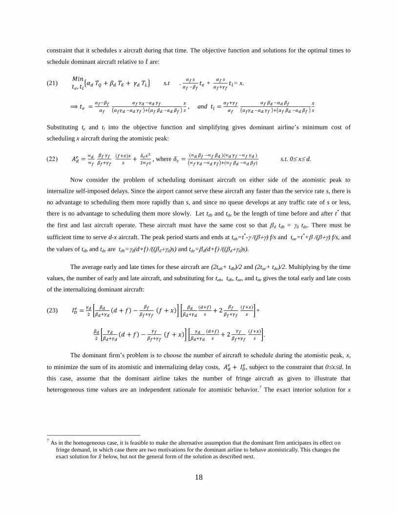
constraint that it schedules x aircraft during that time. The objective function and solutions for the optimal times to
schedule dominant aircraft relative to are:
(21) s.t . + = x.
, and
Substituting te and tl into the objective function and simplifying gives dominant airline’s minimum cost of
scheduling x aircraft during the atomistic peak:
, where s.t. 0xd.
Now consider the problem of scheduling dominant aircraft on either side of the atomistic peak to
internalize self-imposed delays. Since the airport cannot serve these aircraft any faster than the service rate s, there is
no advantage to scheduling them more rapidly than s, and since no queue develops at any traffic rate of s or less,
there is no advantage to scheduling them more slowly. Let tdb and tde be the length of time before and after t* that
the first and last aircraft operate. These aircraft must have the same cost so that d tdb = d tde. There must be
sufficient time to serve d-x aircraft. The peak period starts and ends at tab=t*-/() f/s and tae=t
*+/() f/s, and
the values of tdb and tde are tdb=dd+f/((dd)s) and tde=dd+f/((dd)s).
The average early and late times for these aircraft are (2tab+ tdb)/2 and (2tae+ tde)/2. Multiplying by the time
values, the number of early and late aircraft, and substituting for tab, tdb, tae, and tde gives the total early and late costs
of the internalizing dominant aircraft:
(23) +
.
The dominant firm’s problem is to choose the number of aircraft to schedule during the atomistic peak, x,
to minimize the sum of its atomistic and internalizing delay costs, , subject to the constraint that 0xd. In
this case, assume that the dominant airline takes the number of fringe aircraft as given to illustrate that
heterogeneous time values are an independent rationale for atomistic behavior.7 The exact interior solution for x
7 As in the homogeneous case, it is feasible to make the alternative assumption that the dominant firm anticipates its effect on
fringe demand, in which case there are two motivations for the dominant airline to behave atomistically. This changes the
exact solution for below, but not the general form of the solution as described next.
19
appears below,8 but it is more useful to note that the expressions and have the forms
=cA,fx f x+ cA,xxx2 and = cI,dd d
2 + cI,ff f
2 + cI,xx x
2+cI,dx d x+ cI,fx f x + cI,df d f, where the cA,.. and cI,.. are
coefficients determined by the time-value parameters. It follows that the solution has the form
=(cA,fx f +cI,fx f +cI,dx d)/(cA,xx+cI,xx ). The direct costs experienced by each of the dominant aircraft on average is the
untolled full price, pde[f,d,x]=( + )/d. The total delay cost of operating fringe aircraft in the atomistic peak is
=f(f+x)f/s. Each fringe aircraft experiences full cost of f (f+x)/s in the untolled equilibrium. The equilibrium
number of fringe aircraft is, therefore, . Substituting into the full price and the
result into the fringe and dominant demand curves yields the reduced form for the quantity demanded of dominant
operations of the form, , where c1 and c2 are constant determined by the time values. The expression
for in terms of the underlying parameters is straightforward, but not readily interpretable. The main point is that
this specification with heterogeneous aircraft has fully atomistic, fully internalizing, and mixed equilibria even
though the dominant airline takes fringe demand parametrically. This demonstrates that heterogeneous time values
provide an independent basis for atomistic behavior by the dominant firm, as stated in Proposition 3.
Tolling with heterogeneous time values
Proposition 4: Imposing the same atomistic multiple-step tolling schedule on heterogeneous
dominant and fringe aircraft results in the same constrained-optimal traffic and queuing patterns as
the tolling equilibria with fully atomistic aircraft or with homogeneous dominant and fringe
aircraft. Additional uniform tolls may be necessary to achieve the optimal number of aircraft by
equating their full prices with their marginal social costs. This atomistic tolling schedule enables
the dominant firm to partially internalize self-imposed delay of its aircraft operating during the
atomistic peak.
Without specifing the precise constraints under which the airport authority operates, it is difficult to predict
the outcome in the heterogeneous cases, or determine which toll structures are constrained-optimal. In this section,
the airport is assumed to be constrained to impose a common step-toll schedule for all aircraft. If the airport were
free to impose separate step-toll schedules, it should price the fringe out of the (expanded) period between te and tl,
during which the dominant aircraft operate in the central peak. The dominant airline would schedule all its aircraft
during this period and fully internalize by setting the arrival rate equal to s. The fringe step tolls should treat this as
the central period and step down on either side as before. The case of the common atomistic toll structure is more
interesting because it is more politically feasible and the existing literature is split on whether a common toll can
achieve optimality. This model shows that common atomistic step-toll structures generate the same aggregate traffic
rates and queues as the homogeneous case. The dominant airline obtains the central service intervals that it values
8
, where
20
more highly than the fringe. The dominant airline partially internalizes the self imposed delays of its aircraft
operating during the atomistic peak, and does not double internalize.9 The dominant airline creates some delays to
discourage fringe aircraft from operating during the central periods. Whether the atomistic toll schedule is
constrained optimal, depends on whether it is considered feasible to price the fringe out of the central periods.
Different uniform tolls for dominant and fringe aircraft, or some other policy, are generally required to fully
optimize the quantities of aircraft.
With homogeneous time values, the dominant airline’s cost minimizing number of atomistic aircraft, x,
always satisfies the first order conditions of its optimization problem. With heterogeneous time values, there are
interior solutions (with 0<x<d) that satisfy the first order conditions, but there are also corner solutions with fully
internalizing (x=0) and fully atomistic (x=d) behavior.10
The mixed equilibria occur over a relatively small range of
the cost parameters. The closed form solutions for the number of aircraft, full prices, and tolls in the mixed
equilibrium do not reduce to easily interpretable expressions of the parameters. These solutions are in Appendix A.
The corner solutions are probably more common and their explicit solutions are more manageable.
As in the untolled case, the dominant airline must determine the duration and timing of its operations in the
atomistic peak, te and tl. These values do not vary smoothly with changes in x, because the tolls create discontinuities
in the traffic rates. Let Q[t] be the sum of queuing time costs and tolls, as a function of service completion times.
Then the dominant airline’s problem is to choose te and tl, to minimize , such that
te+tl=x/s. Substituting the optimal te and tl back into the objective and integrating yields . In cases where the
dominant airline operations all occur during the central toll period, the values of te and tl are the same as in the
untolled case, in other cases they are approximately the same. Now define =f (f+x)f/s and . For the fully
atomistic case, the fringe aircraft full price, average cost, and tolls are f , /f, and f - /f,
which simplify to:
(24) , , and .
The fringe toll and full price are greater than they are in the case of homogeneous time values to the extent thatd
exceeds f..
The dominant full price, average cost, and tolls are d , /d, and d - /d, which
simplify to:
9 Double internalization refers to over reaction by the dominant airline when it self-internalizes and faces an atomistic toll. In this
context double internalization would result in too few aircraft or too much peak spreading. 10 Holding other time values constant at reasonable values, there is a narrow range in which the dominant airline’s queuing time
value leads to internal solutions (mixed atomistic and internalizing behavior). When d is close enough to f , the solution is
fully atomistic. As d, increases the cost curve flattens out an eventually transitions rapidly through the mixed equilibria to
the fully internalizing equilibria.
21
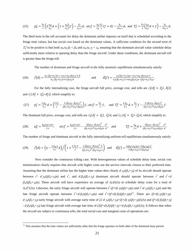
(25) , , and .
The third term in the toll accounts for delay the dominant airline imposes on itself that is scheduled according to the
fringe time values, but has social cost based on the dominant values. A sufficient condition for the second term of
du
to be positive is that both df f <d and df f <d, meaning that the dominant aircraft value schedule delay
sufficiently more relative to queuing delay than the fringe aircraft. Under these conditions, the dominant aircraft toll
is greater than the fringe toll.
The number of dominant and fringe aircraft in the fully atomistic equilibrium simultaneously satisfy:
(26) and .
For the fully internalizing case, the fringe aircraft full price, average cost, and tolls are f , /f,
and f - /f, which simplify to:
(27) , , and .
The dominant full price, average cost, and tolls are d , /d, and d - /d, which simplify to:
(28) , , and .
The number of fringe and dominant aircraft in the fully internalizing uniform toll equilibrium simultaneously satisfy:
(29) and .
Now consider the continuous tolling case. With heterogeneous values of schedule delay time, social cost
minimization clearly requires that aircraft with higher costs use the service intervals closest to their preferred time.
Assuming that the dominant airline has the higher time values then clearly d d/(d+d) of its aircraft should operate
between t*-
d d/((d+d)s) and t
*, and d d/(d+d) dominant aircraft should operate between t
* and
t*+d
d/((d+d)s). These aircraft will have experience an average of d d/(2s) in schedule delay costs for a total of
d d2/(2s). Likewise, the early fringe aircraft will operate between t
*-(f+d) f/((f+f)s) and t
*-d d/((d+d)s) and the
late fringe aircraft operate between t*+d d/((d+d)s) and t
*+(f+d) f/((f+f)s)
11. There are (f+d) f/(f+f)-
d d/(d+d) early fringe aircraft with average early time of (2 d d/(d+d)+(f+d) f/(f+f))/(2s) and (f+d) f/(f+f)
- d d/(d+d) late fringe aircraft with average late time of (2(f+d) f/(f+f) +d d/(d+d))/(2s). It follows that when
the aircraft are subject to continuous tolls, the total social cost and marginal costs of operations are:
11 This assumes that the time values are sufficiently alike that the fringe operates on both sides of the dominant busy period.
22
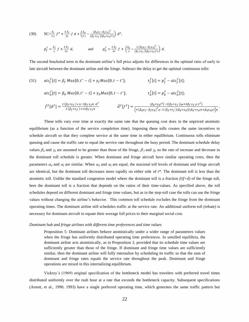
(30) SC= ,
, and .
The second bracketed term in the dominant airline’s full price adjusts for differences in the optimal ratio of early to
late aircraft between the dominant airline and the fringe. Subtract the delay to get the optimal continuous tolls:
(31) ; ;
; ;
.
These tolls vary over time at exactly the same rate that the queuing cost does in the unpriced atomistic
equilibrium (as a function of the service completion time). Imposing these tolls creates the same incentives to
schedule aircraft so that they complete service at the same time in either equilibrium. Continuous tolls eliminate
queuing and cause the traffic rate to equal the service rate throughout the busy period. The dominant schedule delay
values d and d are assumed to be greater than those of the fringe, f and f, so the rate of increase and decrease in
the dominant toll schedule is greater. When dominant and fringe aircraft have similar operating costs, then the
parameters d and f are similar. When d and f are equal, the maximal toll levels of dominant and fringe aircraft
are identical, but the dominant toll decreases more rapidly on either side of t*. The dominant toll is less than the
atomistic toll. Unlike the standard congestion model where the dominant toll is a fraction f/(f+d) of the fringe toll,
here the dominant toll is a fraction that depends on the ratios of their time-values. As specified above, the toll
schedules depend on different dominant and fringe time values, but as in the step-toll case the tolls can use the fringe
values without changing the airline’s behavior. This common toll schedule excludes the fringe from the dominant
operating times. The dominant airline still schedules traffic at the service rate. An additional uniform toll (rebate) is
necessary for dominant aircraft to equate their average full prices to their marginal social cost.
Dominant hub and fringe airlines with different time preferences and time values
Proposition 5: Dominant airlines behave atomistically under a wider range of parameters values
when the fringe has uniformly distributed operating time preferences. In untolled equilibria, the
dominant airline acts atomistically, as in Proposition 3, provided that its schedule time values are
sufficiently greater than those of the fringe. If dominant and fringe time values are sufficiently
similar, then the dominant airline will fully internalize by scheduling its traffic so that the sum of
dominant and fringe rates equals the service rate throughout the peak. Dominant and fringe
operations are mixed in this internalizing equilibrium.
Vickrey’s (1969) original specification of the bottleneck model has travelers with preferred travel times
distributed uniformly over the rush hour at a rate that exceeds the bottleneck capacity. Subsequent specifications
(Arnott, et al., 1990, 1993) have a single preferred operating time, which generates the same traffic pattern but
23
simplifies the calculation of schedule delay. At hub airports, dominant airlines prefer operating at the beginning (for
landings) or ending (for takeoffs) of passenger interchange periods. Airlines often schedule these interchanges at
times that passengers find particularly desirable, so fringe flights may also prefer to operate at these times. On the
other hand, individual fringe aircraft do not have the same rigid scheduling requirements to connect with other
flights. For that reason, it is desirable to determine how robust the previous results are to relaxing the assumption
that fringe flights have the same time preferences as the dominant airline. It turns out that heterogeneous time
preferences do not affect the incentives that aircraft face at the scheduling margin, but do affect the full prices they
face.
No fee equilibria with heterogeneous time values and preferences:
Suppose that the preferred operating times of fringe aircraft are uniformly distributed at rate per minute,
that is less than the service rate s, and the dominant aircraft all have preferred operating time t*. Since the service
capacity is fully used in either a priced or unpriced equilibrium, the length of the busy period is d/(s-) in either
case. When there is no toll and no queue, the fringe aircraft are free to operate exactly at their preferred times. When
a queue develops, however, the distribution of fringe time preferences has no effect on its traffic rates, which from
Equation (3) depend only on time values and the service rate. The fringe aircrafts' best response functions are as
given in Equation (8) with the unsubscripted parameters having the fringe values.
Now suppose that the dominant airline schedules x aircraft in a peak around t*, using the fringe time values
to create a queue sufficient to preempt its preferred operating times, and fully internalizes the self-imposed delays of
its d-x remaining aircraft by scheduling them outside of the peak at rate s-The internalizing aircraft impose no
queuing delays on any aircraft. The length of the atomistic peak period is x/(s-), and the number of fringe aircraft
involved in the peak is f=x/(s-). Equation (22) applies exactly as before to derive , the cost of the dominant
aircraft in the atomistic peak. The beginning and ending of the atomistic peak period are tab= t*- f f fx/(s-)
and tae=t*+ f f fx/(s-). The effective capacity for the internalizing dominant aircraft is now s-so they
must spread out further before and after the atomistic peak. Modifying Equation (28) accordingly gives the
beginning and ending of the entire busy period, tdb=d d/((d+d)(s-)) and tde=d d/((d+d)(s-)). The average
early and late times for these aircraft are (2tab+ tdb)/2 and (2tae+ tde)/2. Multiplying by the time values, the number of
early and late aircraft, and substituting for tab, tdb, tae, and tde gives the total early and late costs of the internalizing
aircraft:
(32) = +
.
This specification generates atomistic behavior by the dominant airline to shift existing fringe traffic out of
the peak, instead of preempting potential entrants. To demonstrate this, we assume in this section only that the
distribution of preferred times for fringe operations is a fixed rate that is perfectly inelastic. The dominant airline
24
chooses x, the number of aircraft to schedule during the atomistic peak to minimize its own total costs + as
given in Equations (22) and (32) subject to scheduling a total of d aircraft and to the number of incumbent fringe
aircraft caught up in the peak period is f=x/(s-). With unresticted cost parameters, this objective function can be
concave or convex and have an interior minimum or a corner solution with x equal zero or d. A sufficient condition
for the second derivative to be negative so that only corner solutions are possible is that:
(33)
which says that if the ratios of dominant to fringe queuing time is small relative to the ratios for early and late time.
Moreover, comparing the full prices for full internalization (x=0) or fully atomistic scheduling (x=d), yields a
sufficient condition that:
(34) and fully atomistic behavior, and
and fully internalizing behavior.
As the density of fringe aircraft operating preferences increases, the range of parameter values for which the
dominant airline behaves atomistically increases. The residual service capacity decreases with the density of fringe
aircraft, requiring dominant aircraft to spread their internalizing aircraft further from their preferred operating time.
The solution for the interior solution is omitted because it is unlikely to occur under the maintained assumption that
dominant airlines value schedule delay more highly than fringe aircraft.
The traffic pattern for the no-toll equilibrium is identical to that given under Proposition 3, but the set of
parameter values for which atomistic behavior is optimal increases. Heterogeneous time preferences raise the cost of
internalization relative to atomistic scheduling because there are additional fringe aircraft surrounding the peak that
use capacity that was available in the homogeneous time-preference case. The qualitative properties of the previous
section’s equilibria still hold. This shows that the model is robust to relaxation of the model’s most restrictive
assumptions.
Tolling with Heterogeneous time values and time preferences
Proposition 6: When the ratio of schedule-time to queuing-time values of dominant aircraft are
sufficiently greater than those of the fringe, the step tolls and tolled traffic patterns are the same as
with heterogeneous time values and homogeneous time preferences. The uniform tolls are
qualitatively similar but quantitatively different. If the schedule-time values are not sufficiently
greater than those of the fringe, then the dominant airline internalizes. Heterogeneous time
preferences increase the range of parameters for which the dominant carrier behaves atomistically.
The solutions for tolls and full prices in terms of the parameters are easily obtainable, but heterogeneity of
dominant and fringe aircraft prevents the solutions from reducing to readily interpretable expressions. For reasons of
space and clarity, the solutions are given in terms of the appropriate derivatives rather than parameters.
25
The schedule delay of fringe aircraft during the atomistic peak differs from the case of homogeneous time
preferences because they operate closer on average to their preferred operating times. For early fringe aircraft, the
smallest schedule delay is zero at tab and the largest is t*-( - )-q[ - ] at - . The queue at - is
( - -tab)(fs/(ff)-s). For late fringe aircraft the largest schedule delay is +q[ ]-t* at and the
smallest is zero at tae. The queue at is (tae- )(fs/(ff)-s). The total cost of operating the fringe aircraft in
the atomistic peak is:
(35)
, where
and
.
This expression simplifies to the form, = cff f2 + cfx f x + cxx x
2.
With the distribution of preferred fringe operating times fixed, the number of fringe aircraft participating in
the atomistic peak depends on how long it takes the airport to serve the dominant aircraft and the fringe aircraft that
they displace. The equilibrium number of fringe aircraft is = /(s-) where solves the dominant airlines
problem of minimizing the full cost of its operations including the costs it imposes on the atomistic aircraft. This
problem is Min subject to = /(s-). As before, this program can have an internal minimum or
corner solutions with fully internalizing behavior or fully atomistic behavior. Given the likely parameter ranges, the
program is convex and the sufficient condition for corner solutions in the tolled case is:
(36) and .
Sufficient conditions for determining whether fully internalizing or fully atomistic behavior minimizes costs are:
(37) and atomistic,
and internalizing.
In the internalizing toll cases, there are no atomistic peaks so the only tolls are the uniform tolls necessary
to optimize the number of operations. Heterogeneous time preferences enable the fringe aircraft to spread out below
the capacity rate, while the internalizing dominant airline fills in the residual capacity. The fringe neither
26
experiences nor imposes queuing delays on other fringe aircraft, but it does impose schedule delay equal to that
experienced by the dominant aircraft furthest from the most preferred dominant operating time. This external cost is
the same no matter when the fringe aircraft operates in the atomistic peak. Fringe tolls and full prices are,
f=pf= . The tolls for dominant aircraft are the same, d=d - /d= . They also
experience schedule delay (on average) in the same amount, so their full price equals pd= This section
maintains the assumption of inelastic demand, but if that assumption were relaxed, the dominant airline would
eventually resort to atomistic behavior to preempt further fringe entry, leading to the tolled equilibria that follow.
In the atomistic cases, the fringe and dominant uniform tolls are fu=f - /f and d
u=d
- /d and the full prices of their operations are pfu=f and pd
u=d , as before. In addition, the
tolling authority should impose step tolls on the aircraft operating in the atomistic peak. All that is required to obtain
the optimal schedule of operations is to treat these aircraft as if they all have the fringe time values. To optimize the
number of operations, the airport authority may either impose a differential step toll to recover the dominant
aircrafts’ higher willingness to pay for operating close to its most preferred time, or it could impose a surcharge on
dominant operations to bring their full cost up to their marginal social cost.
As under Proposition 4, the social optimum is obtained by imposing atomistic continuous-tolls on all
aircraft operating in the atomistic peak and using a uniform toll to equate the full price and marginal social cost of
dominant aircraft operations. The atomistic toll is fff -f Max[0,t*-t] -f Max[0, t+-t*], and the full
price of dominant aircraft is pdfd . When the full price of the dominant and fringe aircraft are
approximately equal, this approach has the advantage of imposing a common toll structure. If the airport authority
wants to impose differential tolls, the dominant toll is ddd -d Max[0,t*-t] - dMax[0, t+-t*].
Capacity implications
Arnott, et al., (1993) compares the full prices, efficiency losses, traffic volumes, and efficient capacity
levels for atomistic bottleneck equilibria with homogeneous traffic facing uniform, coarse, continuous, and no tolls.
It also shows that optimal capacity is self financing, extending the result of Mohring and Harwitz (1962) to the
atomistic bottleneck model with homogeneous traffic. The extensions to the bottleneck model developed here have
several sources of heterogeneity. These include, dominant and fringe airlines, different time values, and different
scheduling time preferences. This section examines whether the properties hold for these extensions.
Proposition 7: Step-tolled airports subject to constant returns to scale are self financing when
dominant airlines behave fully atomistically or fully internalize. Mixed atomistic and internalizing
equilibria do not strictly satisfy the conditions for the self financing result. Continuously varying
(fine) tolls are self financing in any case with constant returns to airport investment.
First consider the multiple-step tolling equilibrium derived above. Equations (7) give the total social cost
function for the step tolls in the form TCs[m,s]=sm2
/s, where sdepends only on the cost parameters and the
number of steps in the toll structure. Summarizing the derivation of Arnott, et al., (1993), we have
27
ATCs[m,s]=sm/s, MSC
s[m,s]=2sm/s, and p
s[m,s]=ATC
s[m,s]+s
[m,s]=MSCs[m,s], which imply that
s[m,s]=ATC
s[m,s]. It follows that the supply function for the step tolled equilibrium is
ps[m,s]= MSC
s[m,s]=2sm/s. The optimal prices and quantities m* and p* satisfy the supply p
s[m,s] and demand
functions m[ps,s] simultaneously. Since the corresponding values for e
.andu in the unpriced and uniform
equilibria equal one, and o for the continuous toll is one half, it follows that p
u*>p
s*>p
o*=p
e* and m
u*<m
s*<m
o*=m
e*.
Defining the social surplus function, , and the efficiency loss,
ELs*
[s]= SSo*
[s]- SSs*
[s], then because the uniform toll is a special case of the step toll, the efficiency losses are
ranked, ELe*
[s]> ELu*
[s]> ELs*
[s]>0. Now define the marginal social benefit of capacity as the derivative of social
surplus with respect to capacity:
(38) ,
The bracketed term equals 1/s whenever, as here, the total cost for fixed traffic volume is proportional to 1/s. The
envelope theorem applies so that total cost is also proportional to 1/s with traffic volume varying optimally. Now
with inelastic demand (which is the likely case for derived demand for landings and takeoffs) and the ordering of
full prices as above, the full cost of operations and the total tolls also have the same ranking. Applying this to the
last line of (38), ranks the marginal benefits as MBu*
[s]>MBs*
[s]>MBo*
[s]. This in turn implies that the optimal
capacity has the order, su*
>ss*
>so*
. For similar reasons, using the assumption that capacity construction costs are
inelastic with respect to capacity, the optimal price and quantities at the optimal capacities are also ordered
pu*
>ps*
>po*
and mu*
<ms*
<mo*
.
The problem of finding the optimal long run price and capacity for the multiple step toll case is to choose
price and capacity to maximize the sum of consumer surplus and toll revenue less capacity construction costs, K[s]:
(39) ,
which has first order conditions:
(40) +
28
These simplify to the following rules: set the average toll equal to the marginal capacity cost, s[m, s]=
ps-ATC
s[m
s[p
s],s
s]=m
s[ p
s] dATC
s/dm, and set capacity so that marginal construction costs equal the marginal
benefit of additional capacity, d K[s]/ds=ms[ p
s] dATC
s/ds. Finally, assuming for convenience that ATC and K are
homogeneous of degree hC and h
K, combining the first order conditions, and applying Euler’s Theorem produces:
(41) .
With the toll equal to the marginal congestion externality, the LHS of (41) is revenue, and the second term on the
RHS is zero because ATC is homogeneous of degree zero. It follows that multiple step tolls cover the construction
cost of the optimal capacity if K exhibits constant returns to scale, i.e., hK=1.
There are two key properties on which the above comparisons of the tolling structures and the self-
financing result depend: that average total costs are inversely proportional to the service rate, s, and that costs are
homogeneous of degree zero in traffic levels and service capacities, m and s. We now consider whether these
properties apply in the cases of dominant and fringe traffic. Note that all the full prices for the uniform and
continuous toll cases where the dominant firm behaves fully atomistically or fully internalizes are inversely
proportional to s and homogeneous of degree zero in quantities f and d and service rate s, except in the fully
atomistic fully heterogenous case. Further note that Equations (5) and (6) imply that the full prices for the step toll
cases are ps[m, s]=N,TC m/s, where m=f+x[d] is the sum of fringe demand and the atomistically scheduled dominant
aircraft and y,z,TC is constant with respect to m and s. The full prices for the step toll cases are also inversely
proportional to s and homogeneous of degree zero in quantities f and d and service rate s. In the mixed equilibria
with homogeneous time values and preferences, the term representing the fraction of the dominant
aircraft behaving atomistically upsets both properties. Thus, in all but the latter case, the dominant-fringe equilibria
satisfy Equation (41), and the relationships apply as before. To see that it is sufficient for these properties to hold
jointly that they hold individually for the dominant and fringe aircraft, define the social surplus and marginal social
benefit as:
(42) , and
.
For the self financing result, consider the program:
(43)
29
which has first order conditions that simplify to:
(44) ,
, and
.
As before, the rules for optimal tolls and capacity are to set the average toll equal to the marginal capacity
cost and choose capacity to equate marginal construction costs and the marginal benefit of additional capacity. Since
the full price of operations is homogeneous of degree zero in mf, md, and s, in all the tolling cases with dominant and
fringe airlines except the mixed equilibrium with homogenous time values and preferences, it follows that the
optimal tolls will pay for the optimal capacity if construction costs are homogeneous of degree one.
Policy discussion and conclusions
The preceding sections extend the deterministic bottleneck model by developing the multiple-step pricing
rules for an atomistic fringe and a dominant airline that controls a significant share of the traffic. The bottleneck
model is more appropriate than the standard model for application to airport traffic because it has a dynamic model
of congestion and it models the aircraft choice of when to operate. Unlike the standard model, delays depend on the
entire prior pattern of traffic during the busy period and current traffic affects delays in subsequent periods. The
bottleneck model captures the effects of aircraft schedules on delays and the effects of delays and tolling on
scheduling. Unlike the standard model in which reducing traffic volume is the only means of lowering congestion,
the bottleneck model also allows internalization of delay by rescheduling aircraft.
The model demonstrates that dominant airlines may or may not internalize their self-imposed delays and
shows the traffic patterns associated with either behavior. Dominant firms are less likely to internalize when they
face a fringe with more elastic demand, when the fringe has similar time preferences, and when the dominant firm
has higher schedule-delay costs. Generally speaking, there is no queue during periods when a dominant firm
internalizes, and there is a queue in periods when the dominant firm is behaving atomistically. Periods with long
queues and mixed dominant and fringe traffic are indicative of atomistic behavior by dominant aircraft. In the
standard model, the dominant airline should pay a fraction of the atomistic tolls equal to the fringe’s share of traffic.
In the bottleneck model with dominant and fringe airlines, fully internalizing dominant aircraft should optimally pay
a fee equal to the marginal cost they impose on each other. This toll does not cause double internalization and has no
effect on the dominant airlines’ behavior because it only brings the full price for infra marginal aircraft up to their
willingness to pay, which then equals their marginal social cost. Tolling these internalizing dominant aircraft
transfers producer surplus to the airport that would otherwise go to the dominant airline, making the surplus
available to fund the costs of capacity. Dominant aircraft that behave atomistically should face the same step tolls as
the fringe, but pay a different uniform toll that accounts for differences in marginal social cost (if any).
30
The results of the model have a number of important policy implications for real-world implementation of
airport congestion pricing. The problems of calculating efficient tolls are overstated. Optimal continuous (fine)
tolling involves valuing the queuing delay experienced in the current untolled equilibrium and imposing a toll
structure with the same pattern over time. While such tolls would be exactly correct only in a deterministic world,
they would be a reasonable approximation of the correct continuous tolling structure in a stochastic world. Daniel’s
stochastic bottleneck model calculates equilibrium tolls that are similar to those in a deterministic model. Another
rule-of-thumb is to calculate the delay cost of the most delayed aircraft in each peak. This is also equal to the
marginal social cost of aircraft operations in a deterministic model. The schedule delay costs of the first and last
aircraft are also equal to the marginal social cost. The model also suggests rules-of-thumb for the optimal multiple-
step tolling structure. The toll increments are constant as the tolls increase or decrease over the peak. All of the
increasing steps have the same duration and all of the decreasing steps have the same duration, while the central
peak is somewhat longer. The step durations are determined by the toll increment, so the entire toll structure can be
determined from an estimate of the cost of the most delayed aircraft and the given number of steps.
The problem of differential tolls between the dominant and fringe aircraft has also been overstated.
Dominant and fringe aircraft should face the same incremental tolls to optimize their scheduling during the atomistic
peak. A different flat toll may be necessary to obtain the appropriate number of aircraft of each type. Other policy
instruments are available to optimize the number of aircraft. For example, many airports currently differentiate
weight-based fees using agreements that offer large airlines lower landing fee rates in exchange for assuming the
risks of revenue shortfalls. Similar arrangements could reduce the uniform tolls of the dominant airlines so that their
full price per operation is efficient. The dominant airlines probably have less elastic demand so that they are less
responsive to toll levels, and the price distortion is minimal. In the bottleneck model, the no-toll traffic levels are
already optimal because the queues increase the full price of aircraft to equal their marginal social cost. This
property depends on the deterministic queuing system, but is approximately true with stochastic queuing. The
internalizing dominant aircraft may be exempted from tolling with no effect on the optimality of aircraft scheduling.
The marginal internalizing aircraft faces the correct full price, because it is the furthest from its preferred operating
time and it imposes no delay other than what it experiences. Other internalizing aircraft (infra-marginal) have full
prices below their willingness to pay, so they retain producer surplus in the no-toll equilibrium. The airport authority
may obtain efficient scheduling of operations by tolling only the atomistic peak with an undifferentiated toll
structure. The traffic levels, however, would not necessarily be optimized.
Mohring and Harwitz’s (1962) and Strotz’s (1965) self-financing of optimal capacity results largely survive
the model’s extension to dominant and fringe aircraft, provided that all aircraft pay the marginal social cost of their
operations. These results support imposition of common multi-step or continuous tolling structures on dominant and
fringe airlines (using the fringe time values), possibly with differentiated flat tolls per operation. Differentiated tolls
are more important when dominant airline internalize, when toll structures have fewer steps, when dominant aircraft
time values differ from the fringe, and when demand for operations is more elastic. Moderately graduated toll
schedules could recapture most of the efficiency loss from congestion and pay for optimally-sized airports.
31
APPENDIX A
The full price for fringe aircraft operations in the tolled equilibria is the marginal social cost, f .
The airport authority sets the fringe toll as the difference between the cost that the aircraft experience, /f, and the
marginal cost. These values have the forms:
(A.1) (f /s+cI,ff ) f +(f /s+cA,fx + cI,fx ) x + cI,df d
and (f /s+2cI,ff ) f +(cA,fx + cI,fx ) x + cI,df d,
where cI,ff , cAfx and cI,df are constants determined by the time values and service rate. Substituting the fringe full
price into its demand function gives the fringe’s optimal demand as a function of the dominant airline’s demand and
number of aircraft scheduled during the atomistic peak. This function is linear in x, d, and :
(A.2) + .
The dominant airline chooses a number of aircraft to schedule during the atomistic peak to minimize the sum of its
internalizing and atomistic aircraft costs. Its problem and solution are: