Working Paper Series No. 2017-06 Cash Burns: An Inventory Model with a Cash-Credit Choice Fernando Alvarez and Francesco Lippi April 3, 2017 JEL Codes: E41, G2 Becker Friedman Institute for Research in Economics Contact: 773.702.5599 [email protected]bfi.uchicago.edu
Transcript
Working Paper Series
No. 2017-06
Cash Burns: An Inventory Model with a Cash-Credit Choice
Fernando Alvarez and Francesco Lippi
April 3, 2017
JEL Codes: E41, G2
Becker Friedman Institute for Research in Economics
We present a dynamic cash-management model where agents choose whether to paywith cash or credit at every point in time. In the model credit usage depends on thecurrent stock of cash, a novel result that matches recent micro evidence on household’spayment choices. The optimality of such decision rule is novel and cannot be obtainedby models where cash-credit decisions are made at the “beginning” of each period. Wediscuss how to use the model to account for cross country-evidence on the intensity ofcredit usage and for several statistics on the size and frequency of cash withdrawals.We use the model to assess the household’s welfare cost of phasing out cash.
JEL Classification Numbers: E41, G2
∗An earlier version of the paper circulated under the name: “A dynamic cash management and paymentchoice model”. We benefited from the comments of the participants to “Consumer Finances and PaymentDiaries: Theory and Empirics”, Ottawa, Canada, 18-19 October 2012. Philip Barrett and David Argenteprovided excellent research assistance.
1 Introduction and overview
We propose a dynamic model of cash-management and means-of-payment choice in which
optimizing households use both cash and credit. Credit is modeled as a payment instrument
that involves a cost but requires no inventory at hand, such as a debit or a credit card, while
use of cash is modeled as a standard inventory problem. A key feature of the model is that
at each moment the agent can choose to pay with either cash or credit. This natural and
realistic feature is an essential novelty of our model which implies that the preferred payment
instrument depends on the stock of cash holdings at the time of the purchase: agents use cash
for a purchase as long as they have cash with them, and use credit otherwise. Agents behave
as if “cash burns” in their hands, a pattern that has been noticed by the empirical literature
(see Arango, Huynh, and Sabetti (2011); Huynh, Schmidt-Dengler, and Stix (2014)). Yet
agents find it optimal to intermittently replenish their cash holdings, and so use both cash
and credit. Our model is the first in the literature to have both simultaneous use of cash and
credit by households, as well as credit use that depends on the level of cash holdings. This
feature is novel and cannot be obtained by models where cash-credit decisions are made at
the “beginning” of each period since, by assumption, those models do not keep track of the
dynamics of cash balances and so the use of credit cannot be conditioned on cash holdings.
Our model provides a simple analytical mapping between the fundamental parameters and
several observable statistics on cash holding behavior, concerning the size and frequency of
cash withdrawals, as well as means of payment choices such as the share of purchases paid
in cash. To illustrate its applicability we use our structural model to assess the household’s
welfare cost of phasing out cash, a policy endorsed by Rogoff (2016) as a measure against
several illegal practices.
We consider a version of the Baumol-Tobin cash inventory model where each cash with-
drawal is subject to a fixed cost augmented with two special features. First, we assume the
agent randomly receives some free withdrawal opportunities, as in Alvarez and Lippi (2009).
This assumption gives rise to a precautionary motive in the demand for cash holdings, such
as an above zero cash-balance at the time of cash withdrawals, a featured extensively found
in household diary and survey evidence. Second, we allow agents to pay for their (exogenous)
constant flow of expenditure using either cash or credit. Our choice of modeling expenditures
as a constant flow has the interpretation of small size purchases. Paying with cash requires
to have positive cash inventory at the time of the purchase, which is costly to accumulate and
which has an opportunity cost, both standard features of an inventory model. Paying with
credit entails a cost per transaction.1 In principle it is possible for the agent to pay all of its
1The choice of cash vs credit based on the size (i.e. dollar value) of purchases has been addressed inboth theoretical and empirical literature, see Arango, Bouhdaoui, and Bounie (2012) and Bouhdaoui and
1
consumption using credit but, as long as there are some free cash withdrawal opportunities,
it will be optimal for the agent to also use cash.
The paper has two main predictions for the use of payment instruments. First, as long
as the cost of cash withdrawals is low enough relative to the cost of credit, the agents never
use credit. They take advantage of their free trips to the bank, possibly some costly trips,
and use cash only. Second, if the cost of cash withdrawals is sufficiently high, then cash is
withdrawn only upon a free cash withdrawal opportunity. In this case the agent uses credit
when she runs out of cash to finance her expenditure, while waiting for the next free cash
withdrawal opportunity. Intuitively, for an agent with cash at hand, the cost of obtaining it
is sunk. As a result, using cash is optimal since the agent pays only the opportunity cost.
Thus, the agent prefers to pay in cash when she has it.
We analytically derive several model predictions and compare them with the cross-country
evidence gathered from households surveys and diary data (as summarized in e.g. Bagnall
et al. (2014)). As mentioned the model predicts that credit is more likely to be used when the
agent is short of cash, a pattern that is robustly documented in micro studies.2 Moreover,
the model has predictions concerning the average share of expenditures paid with cash,
the frequency of cash withdrawals and their average size, the average cash holdings (both
unconditional as well as at the time of cash withdrawals). We show that for low inflation
rates (a realistic assumptions for developed economies), the 5 moments listed above are
functions of 2 parameters only: the normalized cost of credit, namely the ratio between the
cost of credit and the cost of cash withdrawals, and the frequency of the free withdrawal
opportunities. Using data for the US, we discuss how these two parameters can be identified
from observations on e.g. the number of cash withdrawals and the share of cash purchases.
We then compare the model predictions on moments such as the size of cash withdrawals
and the average cash holdings with the data. We show that, in spite of its simplicity, the
model gets the appropriate magnitudes for the observed moments.
Finally, we use our structural model to quantify the cost of a policy that limits household’s
cash usage, a policy endorsed by Rogoff (2016) to fight several illegal activities which are
known to be cash intensive. Our objective is to quantify the welfare cost for households who
are forced to move from their optimal cash-credit share to one where the cash share is zero.
Bounie (2012). Empirically, smaller transactions are more likely to be paid with cash than with credit,which motivates the assumption of a fixed cost per transaction in the literature. Yet, there are many smalltransactions paid with both cash and credit. Our assumption of a constant flow of expenditure thus focuson transactions that are all of the same size and small. It is thus complementary to the explanation in theliterature based on size and it is able to address the choice of means of payments for small size transactions.
2See, for example, Stix (2004), Mooslechner, Stix, and Wagner (2006), Arango, Huynh, and Sabetti (2011),Arango, Hogg, and Lee (2013) and Huynh, Schmidt-Dengler, and Stix (2014). See Appendix A for a briefreview of this evidence.
2
The analysis shows that such cost is small.
Related literature. Many papers in the literature incorporate alternative means of pay-
ments as in the seminal work of Lucas and Stokey (1987) and Prescott (1987). However
such models do not have an explicit inventory theoretical model of money, so they cannot
simultaneously speak to observations such as the fraction of purchases made in cash as well as
cash-management statistics, such the frequency and size of cash withdrawals. Technically, in
this type of models, the cash-in-advance constraint, which is exogenously determined, binds
in every period. As a result, in every period withdrawals occur and all cash is spent. Hence,
statistics such as frequency of withdrawals, size of withdrawals, cash at withdrawals are all
exogenously determined by the choice of the model’s time period. Other models incorporate
both cash management and the choice of means of payments, which ends up being dictated
by the size of the purchases. Examples of such models are Whitesell (1989) or Freeman and
Kydland (2000). Yet while these models introduce cash-management, those choices are all
“within” the period, so that agents cannot choose at every moment whether to use cash or
credit. Hence in these models the optimal use of credit cannot depend on cash holdings, as
the data strongly suggest.3
The closest related models in the literature are Sastry (1970) and Bar-Ilan (1990). Sastry
(1970) is one of the earliest inventory model featuring a sequential cash versus credit choice.
In his deterministic Baumol-Tobin model with no discounting the agent is allowed to use
credit, namely an overdraft (“negative cash”), so that when cash holding reach zero the agent
may continue to consume and postpone the payment of the fixed withdrawal cost. Bar-Ilan
(1990) extends this setup to a dynamic stochastic inventory model. The main difference with
our setup is that the cost of credit in both of these models is assumed to be proportional to
the average stock of credit over the holding period, completely analogue to the opportunity
cost of cash. This implies that the agent using credit will periodically decide to pay the fix
rebalancing cost to keep the average stock of credit under control. Notice that under this
assumption it is infinitely costly not to pay the fixed transanction cost since this implies a
diverging stock of credit. In our setup, in contrast, the cost of credit is proportional to the
expenditure flow, e.g. it is a fixed fraction of the purchase value. Using credit does not
require any fixed cost to “rebalance” the cash credit stock. Credit purchases are immediately
debited on to the agent’s checking account. Our assumption explicitly distinguishes between
the credit technology from the cash technology, and thus makes a credit-only strategy of
purchases feasible for the agent.
3A close analogy between our sequential formulation and these papers’ simultaneous cash-credit choice isfound in the difference between sequential search, as in McCall’s model, versus simultaneous search, as inStigler’s search model. See Sargent’s (1987) chapter 2 for a description of the two types of search models.
3
Organization of the paper. The structure of the paper is as follows. We illustrate the
model’s key idea in Section 2 with a simple deterministic steady-state model. Section 3 intro-
duces uncertainty and a proper dynamic treatment of the inventory problem with payment-
choice. This section characterizes the conditions under which both cash and credit are used
by the agents. Section 4 derives the model implications for the frequency and size of cash
withdrawals and the intensity of credit usage. We discuss some cross-country evidence to
illustrate how the model can be calibrated to actual economies. In Section 5, we use our
structural model to quantify the cost of a policy that imposes a zero-cash usage restriction.
Section 6 extends our model by allowing for a random cost of cash withdrawals, a feature
which appears desirable for empirical applications. Section 7 concludes.
2 A deterministic model with means of payment choice
This section presents a steady-state deterministic model that highlights the main mechanism
of the dynamic stochastic model of Section 3. Indeed some key formulas from this simple
model coincide with, or are close to, the more complex decision rules of the stochastic model.
The main counterfactual prediction of the deterministic model is the lack of a precautionary
motive, so that real balances are always zero at the time of a withdrawal.4
Consider an agent who consumes e per unit of time and can pay for this using cash or
credit. If she pays with credit she incurs a direct cost γ per unit bought. The cost γ can be
understood as the time cost of using credit for small value transactions. The technology to
withdraw cash (from an interest bearing checking account) is as follows: at any time the agent
can pay a fixed cost b and replenish her cash balances which, as in the canonical Baumol-Tobin
model, are subject to an opportunity cost R (e.g. forgone interest on deposits). Moreover,
the agent has p ≥ 0 withdrawals per period that come for free. The latter assumption is
a simple parametrization of the technology for the cash withdrawals, proxying e.g. for the
number of ATMs (cheap withdrawals) available to the agent.
To understand the nature of the optimal policies considered below notice that in a deter-
ministic setup an agent with positive cash balances will not pay the fixed cost b to withdraw
cash unless cash balances are zero. Consider now the decision of whether to purchase goods
using cash or credit. For an agent with positive cash balances m > 0 it is not optimal to pay
the cost γ e to use credit, since the cost of acquiring the cash is sunk at this time.5 For an
agent with zero cash balances m = 0, there are two possible choices: the first one is to pay
4Readers familiar with continuous time impulse control problems may move directly to Section 3.5Another possibility is to use credit and deposit the cash to earn a higher interest. With a fixed cost for
depositing this is not optimal unless the cash balances are very large, a situation that will not occur alongan optimal path.
4
the cost γ e and finance consumption using credit, waiting until the next free withdrawal
opportunity to replenish cash balances. The second choice is to pay the fixed cost b and
withdraw cash. We first separately describe the solution of these two cases and next analyze
the best choice among the two.
2.1 The deterministic cash-credit model
Consider an agent who finances her expenditures using cash, and who pays with credit once
cash balances are depleted. Assume further that no costly withdrawal ever takes place so
that b is never paid and the number of withdrawals n equals the number of withdrawals that
come for free p. After a cash withdrawal of size W = m∗, she spends τa = m∗/e units of
time paying for consumption with cash, incurring an opportunity cost Rm∗/2, where m∗/2
is the average cash balance conditional on m > 0 and R is the opportunity cost of cash–
which includes the nominal interest rate as well as the probability of cash theft. After cash
balances hit zero, the remaining time until a free withdrawal opportunity, denoted by τr, is
given by τr = 1/p −m∗/e. Notice that τr + τa = 1/p. The steady state cost in every cycle
of duration 1/p can be written as: τr γ e + τa R m∗/2. The cost per unit of time is thus
p τr γ e + p τa R m∗/2. Thus the minimized cost of the strategy that uses both cash and
credit is:
vr(R, γ, p, e) = min0≤m∗≤e/p
p
[
(1/p−m∗/e) γ e + (m∗/e) R e(m∗/e)
2
]
,
subject to the constraint that the time spent using credit is non-negative, i.e. m∗/e ≤ 1/p.
We denote by s the “cash share”, namely the ratio of the expenditure paid with cash to total
expenditure per unit of time, given by
s =τa
τa + τr= min
{
pm∗
e, 1
}
.
Denoting the average real balances by M and using the cash share s we can write M =
s m∗/2. The cost minimizing policy yields m∗
e= W
e= min
{
1p, γ
R
}
, s = min{
1 , γ pR
}
,
Me= min
{
12 p
, p2
(
γR
)2}
which imply
vr(R, γ, p, e) =
(
1− γ p2 R
)
γ e if R ≥ γp
(
R2 p
)
e if R < γp
(1)
5
When R ≥ γp credit is “cheap”, so that both cash and credit are used. When R < γp credit
is expensive and it is not used.
2.2 Deterministic Baumol-Tobin model with p free withdrawals
Let us consider a modified Baumol-Tobin model in which the agent pays only for the with-
drawals in excess of the p free adjustments per period.6 The agent chooses a withdrawal
of size m∗ when cash balances are exhausted (m = 0). The policy implies an average cash
balance M = m∗/2 and a number n = e/m∗ of cash withdrawals. The agent’s choice of m∗
gives the minimized cost function
va(R, b, p, e) ≡ minm∗
[
Rm∗
2+ bmax
( e
m∗− p , 0
)
]
.
where the cost is given by the sum of the opportunity cost of cash holdings and the cost
associated with cash withdrawals in excess of p. The optimal policy for a technology with
p ≥ 0 is m∗
e= 1
p
√
min(
2 b p2
e R, 1)
. For p > 0 there is no reason to have less than p
withdrawals, since these are free. Hence, for R < 2p2b/e the agent will choose a constant
level money holdings: m∗ = e/p. Note that the interest elasticity of money is zero over this
range, while it is equal to 1/2 if R > 2p2b/e. The average withdrawal size W and the average
cash balances satisfy: W = m∗ , M = 2 W = 2 m∗ . Replacing the optimal m∗ choice in
the cost function yields
va(R, b, p, e) =
(√
2 R be− p b
e
)
e if R ≥ 2 p2 be
and n > p
(
R2 p
)
e if R < 2 p2 be
and n = p
(2)
where the top branch gives the cost for the case in which the number of withdrawals exceeds
p. Note that in this deterministic setup an agent with positive cash balances will not pay
the fixed cost b to withdraw cash unless cash balances are zero.
2.3 The full deterministic problem
We now analyze the conditions under which it is optimal to use credit instead of with-
drawing fresh cash when m = 0. To do so we compare the steady-state cost of the two
policies computed above. The value function for the problem is then v(R, b, γ, p, e) =
6See Alvarez and Lippi (2009) for a more detailed analysis of this model and Appendix C for estimates ofcash theft probabilities, which are a component of R, in Italy and the US.
6
min {va (R, b, p, e) , vr (R, γ, p, e)} . We define the threshold function b, as the value of b
that equates the two minimized costs: va(R, b, p, e) = vr(R, γ, p, e) . We have that
b(R, γ, p, e) =γ2
2 Re . (3)
which implies that credit is used when b ≥ b provided that γp ≤ R.7 If b ≥ b and γp > R
then credit is not used and n = p. Finally, for b < b credit is not used and n > p since some
costly withdrawals in access of the p free withdrawals are now optimal .
The next proposition summarizes the behavior of the deterministic model. It considers
two cases depending on whether γ ≷ 2p b/e, and for each case it analyzes optimal policy as
a function of R.
Proposition 1. Let p > 0 and γ > 0. Then W/M = 2/s and
If γ > 2 p be, then
if R ∈(
0 , 2 p2 be
]
−∂ logM/e∂ logR
= 0 only cash used n = p s = 1
if R ∈(
2 p2 be, γ2
2 b/e
]
−∂ logM/e∂ logR
= 1/2 only cash used n > p s = 1
if R ∈(
γ2
2 b/e, ∞
)
−∂ logM/e∂ logR
= 2 cash & credit used n = p s = γp/R
Otherwise, i.e. if γ ≤ 2 p be, then
if R ∈ (0, γp] −∂ logM/e∂ logR
= 0 only cash used n = p s = 1
if R ∈ (γp , ∞) −∂ logM/e∂ logR
= 2 cash & credit used n = p s = γp/R
The proposition illustrates three robust properties of the model. First, the model has only
two parameters, γp and p2 b/e, as the alert reader will have noticed. In the modified Baumol-
Tobin model the shape of the money demand depends only on b ≡ p2 b/e. For a given value
of b, the cash-credit aspect of the model depends only on γp. We will see that this property
continues to hold in the stochastic model analyzed below. Second, for credit to be used it is
necessary that the cost of a withdrawal is above the threshold defined in equation (3). If b > b
then the agent uses both cash and credit to finance her consumption, and costly withdrawals
are never used. The condition for the optimality of credit depends on a combination of the
7 The expression for b comes from equating: vr = γe[1− γp/(2R)] with va = e√
2 R b
e− pb.
7
fundamental parameters R, b and γp which, intuitively, imply that the cost of cash (which is
increasing in R and b) must be high relative to the cost of credit (which is increasing in γ
and p). Third, the interest rate elasticity of money demand is increasing in the interest rate.
There are two cases: the first corresponds to a large cost of credit (γp > 2 p2 b/e), in which
case there are three qualitatively different behavior depending on the level of interest rates.
If interest rates are very low, credit is not used and n = p, resulting in an elasticity of zero.
For intermediate level of interest rates, credit is not used, but n > p, so the local behavior is
identical to Baumol-Tobin, producing an interest rate elasticity of 1/2. For higher interest
rates, both cash and credit are used. The interest rate elasticity is higher here because both
the cash share as well as the size of the withdrawals react to interest rates. If instead the
cost of credit is low (γ ≤ 2 p b/e) there is no intermediate case, since credit always dominates
the Baumol-Tobin type of behavior.
3 A dynamic stochastic model with means of payment
choice
In this section we solve a discounted, stochastic dynamic problem which joins the optimal cash
management problem with the optimal choice of means for payment. As in the deterministic
problem the agent faces a total consumption per unit of time e > 0 which must be paid with
either cash or credit: at each instant the agent can choose to pay in cash c ∈ [0, e] and to
pay the remaining e− c using credit. If the payment is made by credit, the agent pays a flow
cost γ per dollar.8 The quantity γe can be interpreted as the “handling” and “verification
and authorization” costs estimated in Klee (2008) using grocery receipts data. The state of
the agent’s problem is given by her real cash balances m ≥ 0. If m = 0 either cash must be
withdrawn or credit has to be used. If m > 0 the agent faces a cash/credit choice. The law
of motion of real balances is then dm = − (c+ mπ) dt provided that no adjustment takes
place, where π is the constant inflation rate. The agent can adjust her cash balances paying
the fixed cost b ≥ 0. Additionally, there is a Poisson process with constant arrival rate p ≥ 0,
which describes the arrival of a free adjustment opportunity. When such an opportunity
occurs the agent can adjust her cash balances at no cost. As standard in monetary models,
we assume that holding cash m entails an opportunity cost Rm per unit of time, where R
can be interpreted as the sum of the nominal interest rate plus a probability that cash is
lost or stolen. We assume that the agent minimizes the expected discounted cost, using a
constant discount rate r ≥ 0. There are three substantive differences between the model
8It turns out that, given that all expenditures are of the same size, it is equivalent to assume that thereis a fixed cost, since the optimal policy will be of the bang-bang type.
8
analyzed in this section and the steady-state deterministic model of Section 2. First, we take
into account explicitly the role of inflation, as can be seen in the law of motion. Second, the
free adjustment opportunities arrive stochastically. Third, real costs are discounted by an
appropriate rate r.
Formally we denote by V (m) the minimum expected discounted cost of supporting a
constant flow of expenditure e when the current real cash at hand is m ≥ 0. The function
V , defined in V : R+ → R+ must solve the following functional equation:
0 = min
{
min0≤c≤e
Rm+ γ[e− c] + pminz≥0
[V (z)− V (m)]− V ′(m)(c+ πm)− r V (m) ,
b+minz≥0
V (z)− V (m)
}
for all m ≥ 0 . (4)
The outer min{·, ·} in the functional equation (4) chooses between two strategies. The term
in the first line represents the case where no costly withdrawals (that involve paying the
fixed cost b) occur, although random free withdrawal opportunities may arise, and the agent
chooses what fraction of her consumption to pay in cash versus credit. This is a standard
continuous time Bellman equation, with flow cost Rm+ γ(e− c) and with expected changes
due to either the arrival of the free adjustment opportunity or to the depletion of cash. The
minimization with respect to c describes the agent’s choice of the optimal means of payment.
The term in the second line corresponds to the strategy of exercising control, i.e. paying
the fixed cost b and adjusting cash holdings. For each m the value function is equal to
the value of the strategy that yields the minimum cost. Whenever an adjustment is made,
either paying the cost b or when a free adjustment opportunity arrives, the post-adjustment
quantity of cash is chosen optimally. The optimal policy for the problem in equation (4)
consists of deciding for each m ≥ 0 whether a costly withdrawal is made or not and, if no
adjustment is made, which payment instrument (cash or credit) to use. Notice that this
formulation does not impose any restriction concerning when the adjustments takes place
or when different payment instruments are used. We maintain the following assumption
throughout this section.
Assumption 1. We let b ≥ 0, γ ≥ 0, π ≥ 0, p ≥ 0, and r + p+ π > 0, e > 0, R > 0.
If e = 0 the problem becomes uninteresting since there is no expenditure to finance. The
parameters b and γ are costs, and p a probability rate, so they must be non-negative. The
requirement that r+ p+π > 0 and R > 0 are important. For instance, if r+ p+π = 0 there
is no intertemporal incentives to use cash.9
9 While here we treat R and r, p, π as independent parameters the value of R and r + p + π can indeed
9
3.1 Two candidate policies
It will turn out that the optimal policy of the problem depicted in equation (4) is one of two
types, depending on parameters. We refer to one of the policies as a cash-burning policy,
defined as follows:
Definition 1. We define a m∗-cash burning policy as a threshold m∗ ≥ 0 for which:
1. Credit is only used when m = 0, and cash is used for every m ∈ (0, m∗).
2. Cash is only adjusted when a free adjustment opportunity arrives.
3. Immediately after a cash adjustment, cash holdings m take the value m∗.
Note that the value of following a m∗-cash burning policy is the function V : [0, m∗] → R+
that satisfies:
(r + p)V (m) = mR + pV (m∗)− V ′(m)[πm+ e] for all m ∈ (0 , m∗] and (5)
(r + p)V (0) = γe+ pV (m∗) (6)
The first one is the standard Bellman equation, where we assume everything is paid in cash.
The second equation says that at m = 0 agents use credit and wait for a free withdrawal
opportunity. For completeness we define an alternative policy, which we refer to as a modified
Baumol-Tobin (BT) policy:
Definition 2. We define a m∗-Baumol-Tobin policy as a threshold m∗ ≥ 0 for which:
1. Credit is never used.
2. Cash is adjusted when either a free adjustment opportunity arrives or when m = 0.
3. Immediately after a cash adjustment, cash holdings m take the value m∗.
We briefly comment on the differences between the two polices. There is a sense in which
cash burns in the agent’s hands under both policies, since in both cases, as long as it is
available (m > 0), cash is the preferred means of payment. Note that when a m∗-Baumol-
Tobin policy is followed the o.d.e. in equation (5) holds in the range of inaction (0, m∗].
However, under this policy the boundary condition at m = 0 is given by:
V (0) = b+ V (m∗) . (7)
be related –for instance r+ π should be the shadow nominal interest rates. We return to this relationship inthe next section.
10
For a cash burning policy to be optimal, i.e. to solve the problem in equation (4), one
needs to establish that it is optimal to pay with cash at m ∈ (0, m∗] and with credit at
m = 0, where the optimal withdrawal m∗ must be determined. Finally, it has to be shown
that at m = 0 it is optimal to wait for a free adjustment opportunity (instead of paying b to
withdraw). Likewise, for a BT policy to be optimal, i.e. to solve the problem in equation (4),
one needs to establish that it is never optimal to pay with credit and that at m = 0 it is
optimal to pay b and choose the optimal withdrawal level m∗ (see Appendix B for a formal
proof that all these properties are verified under the optimal policy).
Note that the feasible policies consistent with equation (4) are much broader than the
two candidate policies defined above. For instance, one could consider a policy in which
credit is used for some time at m = 0 and a costly withdrawal occurs after T periods unless
a free withdrawal arrives. Such a policy is the optimal one in the models of Sastry (1970)
and Bar-Ilan (1990). Interestingly, as we explain below, the optimal policy for the problem
in equation (4) will either take the form of a modified Baumol-Tobin one (where credit is not
used) or of a cash-burning policy.
3.2 Characterizing the optimal cash-credit choice
The next proposition characterizes the optimal cash vs credit choice. Appendix B provides
the proof as well as a detailed analytic characterization of decision the rules, including ap-
proximate solutions for m∗ in the case of zero inflation.
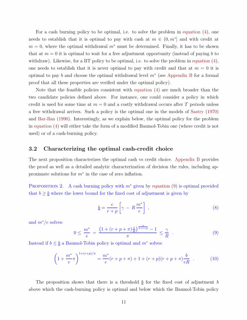
Proposition 2. A cash burning policy with m∗ given by equation (9) is optimal provided
that b ≥ b where the lower bound for the fixed cost of adjustment is given by
b =e
r + p
[
γ − Rm∗
e
]
, (8)
and m∗/e solves:
0 ≤m∗
e=
(
1 + (r + p+ π) γR
)π
π+r+p − 1
π≤
γ
R. (9)
Instead if b ≤ b a Baumol-Tobin policy is optimal and m∗ solves:
(
1 +m∗
eπ
)1+(r+p)/π
=m∗
e(r + p+ π) + 1 + (r + p)(r + p+ π)
b
eR. (10)
The proposition shows that there is a threshold b for the fixed cost of adjustment b
above which the cash-burning policy is optimal and below which the Baumol-Tobin policy
11
is optimal. When b > b the optimal policy consists of using both cash credit. A withdrawal
of size m∗, as determined by equation (9), occurs every time a free withdrawal opportunity
arises. When cash eventually hits m = 0, then it is optimal to finance consumption using
credit until a free opportunity for a cash withdrawal arises. Thus, under cash-burning n = p
and the fixed cost b is never incurred by the agent. Conversely, when b < b credit is not used
and the optimal policy at m = 0 consists in paying the fixed cost b to make a withdrawal
of size m∗, as determined by equation (10). Notice that the optimal threshold b defined
in equation (8) summarizes the effect of all fundamental parameters (γ, R, π, r, p, e) into
one single function that determines the nature of the optimal policy and, in particular, the
optimality of using credit. Intuitively, equation (8) implies that the use of credit is optimal
whenever the cost of using cash (which is increasing in R and b, and decreasing in p) is high
relative to the cost of credit usage (which is increasing in γ).
Finally we notice that the optimal policy is of the bang-bang type, in the sense that using
credit strictly dominates, or is dominated by, the use of costly withdrawals. This result differs
from the ones of Sastry (1970) and Bar-Ilan (1990) where the use of some costly credit as
well as some costly withdrawals is optimal. As mentioned in the introduction, this difference
originates on the way the cost of credit is modeled in these papers compared to ours. We
assume that the cost of credit is proportional to the expenditure flow : γe. They instead
assume the cost of credit to be proportional to the stock of accumulated credit, the exact
analogue of “negative cash”, which periodically requires the agent to pay the fixed cost b
to rebalance the credit cost which would otherwise diverge. We see our assumption as a
reasonable description of the case of revolving credit (credit that is automatically debited on
the agent’s checking account at the end of the holding period).
The next proposition analyzes how the threshold b changes as a function of the parameters:
Proposition 3. The function b ≥ 0 is bounded above by eγ/(r+ p) and it is homogenous
of degree one in (γ, R). Moreover
∂b
∂γ> 0 with lim
γ→0b = 0 and lim
γ→∞b = ∞ ,
∂b
∂R< 0 with lim
R→0b =
e γ
(r + p)and lim
R→∞b = 0 ,
limr+p→0
b =eR
π2
[(
1 +γπ
R
)
log(
1 +γπ
R
)
−γπ
R
]
=γ2
2Re + π o
(
γ2
R
)
≥ 0 ,
limπ→0
b =eγ
r + p
[
1−log(
1 + (r + p) γR
)
(r + p) γR
]
=γ2
2Re + (r + p) o
(
γ2
R
)
≥ 0 ,
∂b
∂π< 0 , lim
π→∞b = 0 ,
∂b
∂(r + p)< 0 , and lim
r+p→∞b = 0 .
12
The proposition shows that the critical threshold b is increasing in the credit cost γ
and decreasing in the opportunity cost of using cash R. In addition, by varying γ/R the
threshold b ranges from zero to infinity. The approximations in the second to last line shows
that if γ2/R is small then b coincides with the one of the deterministic model. Moreover, the
threshold b is decreasing in inflation: higher inflation increases the range of parameters for
which the cash burning policy is optimal. Notice however that for finite values of γ and R,
b > 0 which implies that there exists a sufficiently small value of b > 0 that makes the use of
credit dominated by a cash-only policy. Also notice that in our model a credit-only policy,
i.e. one where cash is not used, does not occur as long as p > 0. The last two results suggest
that the use of cash is very resilient: technical innovations that reduce the cost of credit are
also likely to reduce the cost of cash withdrawals (increase p and or lower b) so that cash
usage remains convenient for agents.
4 Model predictions about observable moments
Next, we consider several statistics of interest generated by a household who follows the
optimal policy described above. We denote by s ≡ c/e the cash share, namely the long run
average fraction of purchases paid with cash. We denote by M the average cash holdings of
the household. This is the expected value of real balances under the invariant distribution
of real balances (m) implied by the optimal decision rules. We let n be the expected number
of withdrawals per unit of time and W the expected size of withdrawals under the invariant
distribution. Finally, we let M be the expected value of cash at the time of a withdrawal.
Table 1 reports sample means for each of these moments for a few OECD economies, taken
from household surveys and diary data by Bagnall et al. (2014) and Alvarez and Lippi
(2013).10 One main difference is a markedly smaller fraction of expenditures that is paid in
cash in the US (or France, around 20% of total expenditure) relative to e.g. Germany (or
Italy, where it is around 50% of the total expenditure). The higher cash use in Germany and
Italy is also reflected in higher values of cash holdings (M/e).
Next, we illustrate how those statistics map into the fundamental parameters of the
dynamic model considering two cases: first a household who follows the cash burning policy,
which is optimal when b > b, so that credit is used. Second, the case when b < b and credit
is not used. We stress that the main empirical appeal of the cash burning policy is twofold.
10 Bagnall et al. (2014) analyze data from large-scale payment diary surveys conducted between 2009 and2012 in Australia, Austria, Canada, France, Germany, the Netherlands and the United States that enableinternational comparisons. Alvarez and Lippi (2013) focus on Austria and Italy.
13
Table 1: Selected moments on cash holding patterns
Fra Ger Ita USCash balances (median), M/ed 1.3 2.6 6.5 0.6Number of cash withdrawals, n 96 57 55 64Withdrawal size (median), W/M 1.7 2.1 1.3 2.3Cash at withdrawals (median), M/M - 0.3 0.4 0.7Cash share of expenditures, s = c/e 0.15 0.53 0.52 0.23
The data source is Bagnall et al. (2014) Tables 1 to 4. Entries are sample means (unless otherwiseindicated). The Italian data are from Alvarez and Lippi (2013) for household who posses a ATM card.Cash balances M/ed are measured relative to total expenditures per day, ed = e/365. The number ofcash withdrawals is per year.
First, it is consistent with the data as it rationalizes the use of both cash and credit. And,
second, the policy aligns with the empirical observation that households are more likely to
use credit when their cash balances are running low, a fact that is amply documented in
Arango, Huynh, and Sabetti (2011); Kosse and Jansen (2012); Huynh, Schmidt-Dengler, and
Stix (2014); Arango, Bouhdaoui, and Bounie (2012). The next proposition summarizes the
main results and closed form expressions for the observables focusing on the simple case of
zero inflation π = 0.
Proposition 4. Let s ≡ c/e denote the cash share., i.e. the share of purchases paid with
cash. For the cash-burning and the Baumol-Tobin policy we have:
(i) Cash-burning policy. Let r + p > 0, π = 0, R > 0 and b ≥ b. Then
n = p , s = 1−
(
1 +γ(r + p)
R
)− p
r+p
,M
e=
m∗
e−
s
p, W =
e
ps ,
thus, using equation (9) with π ↓ 0 gives m∗
e= 1
r+plog(
1 + γ(r+p)R
)
≥ 0. For r ↓ 0 these
expressions are simple functions of γp/R:
s =γpR
1 + γpR
,M
e=
1
p
[
log(
1 +γ p
R
)
− 1 +(
1 +γ p
R
)−1]
and
W
M=
1(
1 + Rγ p
)
log(
1 + γ pR
)
− 1and M/M = 1 .
(ii) Baumol-Tobin policy. Let R > 0, p > 0, π = r = 0 and b < b. Then s = 1 and
14
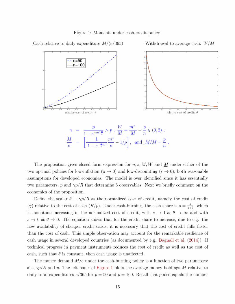
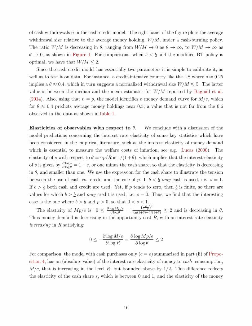
Figure 1: Moments under cash-credit policy
Cash relative to daily expenditure M/(e/365) Withdrawal to average cash: W/M
share of cash expenditure0 0.1 0.2 0.3 0.4 0.5 0.6
cost
in%
ofdailyconsumption
0
2
4
6
8
10
12
14
The “exact” cost function in the left panel assumes inflation equal to 2 percent and a timediscount r = 0.02. The right panel uses, for each value of s on the x-axis, the correspondingvalue of γ implied by Proposition 4 under the assumption that n = 50 and R = 0.02.
Next we quantify the cost of credit, γ, using the relation between s and γp/R from
Proposition 4 and that p = n. Assuming a nominal interest rate of 2 percent (the opportunity
cost of cash R), and n ≈ 50 per year as measured in the US and Germany, the model gives
that γ = sR(1−s)n
. Using this equation shows the cost of credit γ to be a tiny number, about
4 basis point for s = 0.5 and 1.3 basis point for s = 0.25. The right panel of Figure 2 plots
the implied cost per year of imposing the zero cash restriction assuming n = 50, R = 0.02
and computing the cost of credit γ implied by each level of s. As suggested by the estimates
discussed before, the cost of implementing Rogoff’s restriction appears tiny over the range of
cash share values observed in the data: for a household with an annual consumption of 40K
the cost is approximately 10 dollars per year in Germany, where the cash share is around
50%, it is about 2 dollars in the US where the cash share is around 25%.
Two remarks are useful to put the above figures in perspective. First, the magnitude of
the cost scales proportionally with the value of γ as equation (12) shows. It is thus useful to
note that the small estimates for γ discussed above, in the order of a few basis points, are
likely affected by our specific modeling assumptions, in particular the assumption that all
cash withdrawals are free under the cash-burning policy. Modifying this assumption, as done
in the extension of Section 6, will likely increase the cost of credit. For arbitrary values of the
cost of credit the left panel of Figure 2 can be used to gauge the cost of the zero-cash policy
at any given level of the cash share. Second, our estimated costs of phasing out cash is borne
19
by households who already possess the credit technology. A more encompassing measure of
the social cost would also include the costs borne by the currently unbanked (about 7 percent
of households in the US, see FDIC (2015)).
6 An extension: random variation in fixed cost
The model of Section 3 is very stark in that credit is used at m = 0 provided that the fixed
transaction costs is sufficiently high (b > b) in which case we have that M = M and n = p.
Instead, if the transaction cost is sufficiently low (b < b) credit is never used, i.e. s = 1 and
the model becomes the Baumol-Tobin with random free withdrawal opportunities discussed
in Alvarez and Lippi (2009). The prediction that the cash share is either zero or 1 seem too
stark against the data. In particular, there is substantive evidence, based on micro data, that
the amount of cash at the time of withdrawals is smaller than the average cash balance, i.e.
M < M . We show in this section that allowing the fixed cost b to be random and persistent
allows to account for this fact while retaining the other features of the model. The variation
in b implies that agent follows a cash-burning policy when she faces a high cash withdrawal
cost, while she follows a Baumol-Tobin policy when the cost of cash withdrawals is below a
critical threshold. The analysis can equivalently be conducted assuming the cost of credit to
be random.
In particular we assume that there is a Poisson process with constant intensity λ whose
occurrence indicates that a new value of b has been drawn. This Poisson process is inde-
pendent of the one for the arrival of the free adjustment opportunities. The new values for
the cost b are drawn from the cumulative distribution function F : R → [0, 1]. Conditional
on a change in the value of the fixed cost, the new value b is assumed to be independent of
the current value b. In this case the value function has two arguments, (m, b), so we write
it V : R2+ → R+. We denote by primes the derivative of V with respect to m. The value
function solves the following functional equation:
0 = min
{
min0≤c≤e
Rm+ γ[e− c] + pminz≥0
[V (z, b)− V (m, b)] + λ
[∫
V(
m, b)
dF(
b)
− V (m, b)
]
−V ′(m, b)(c+ πm)− r V (m, b) , b+minz≥0
V (z, b)− V (m, b)
}
∀ (m, b) ∈ R2+ (13)
The interpretation of the terms in this functional equation is analogue to the one in equa-
tion (4): the outer min operator compares the value of using credit with the value of paying
the fixed cost and replenishing cash balances. There are two differences. First, as mentioned
above, b is also part of the state. Second, in the first term there is an extra expression given
20
by the contribution to the expected change of the value function due to the change in the
cost from b to a value drawn from the distribution with c.d.f. F .
In what follows we proceed, based on the analysis of the special cases analyzed in the
previous section, by constructing a solution for a type of cash-burning policy which combines
the two cases analyzed above.
Definition 3. A threshold cash-burning policy is defined by a cost threshold b and a cash-
target function m∗. For all m > 0 and all b ≥ 0 the agent uses only cash. If m = 0 the agent
withdraws cash when 0 ≤ b ≤ b, and uses credit when b > b. For all (m, b) cash balances are
set equal to m∗(b) every time that a free adjustment opportunity arrives. Additionally, cash
balances are set to m∗(b) if m = 0 and b ≤ b.
Hence b is the critical threshold so that at m = 0 the agent uses credit if b < b and uses
cash otherwise. Appendix C gives a detailed characterization of the value function for this
problem under a threshold cash-burning policy. We use this extended model in a calibration
that illustrates how it can produce cash management behavior featuring both cash and credit
usage and where the amount of cash at the time of a withdrawal is smaller than the average
cash holdings, i.e. M < M . As mentioned, the latter feature is seen in the data but is not
produced by the model with a constant cost of withdrawal studied in Section 3.
A quantitative assessment. As a benchmark, we use the observable statistics for Italian
households which were summarized in Table 1. We focus on households that own an ATM
card, a group for which the cash-credit margin is feasible.12 For this group the data shows
that share of cash expenditures is close to 50 percent of total (non-durable) expenditures and
that the average currency holdings is about 6 days of expenditures. Moreover, it shows that
the amount of cash at the time of withdrawal relative to the average money balances M/M is
around 0.4, that the ratio of the average withdrawal to the average money balances is about
W/M is 1.3 and that the households with ATM withdraw cash about 50 times per year.
Table 2 reports the comparable moments predicted by 3 cash management models. For
comparison, all three models are calibrated to reproduce the same value of average currency
holdings (M/e = 6) and the same number of cash withdrawals (n = 53). Column [1] uses
the cash-only model described in part (ii) of Proposition 4. This model corresponds to the
best cash management strategy when the (fixed and deterministic) withdrawal costs are low
(b < b), so that credit is not used. As discussed in Alvarez and Lippi (2009) this model has
essentially 2 independent parameters, p and bp2
eR, which we use to target the mean level of
cash holdings and the number of withdrawals (first two lines of the table). The predictions
12 In Italy the vast majority of ATM cards also serve as debit cards.
21
Table 2: Selected moments on cash holding patterns: different models
Model[1] [2] [3]
cash-only cash-credit mixedAverage Currency M/ed 6 6 6Number of cash withdrawals n 53 53 53Withdrawal size W/M 1.1 0.9 1.0Cash at withdrawals M/M 0.6 1.0 0.8Cash share of expenditures s 1.0 0.8 0.9
Cash balances M/ed are measured relative to total expenditures per day, ed = e/365. The number ofcash withdrawals is per year. The parameters for model [3] are chosen to broadly match frequency ofwithdrawals and size of money holdings. The low value of b is 1% percent of daily consumption, the highvalue is 30%. The rate at which b changes is λ = 250 times per year.
for the other moments can be seen as an over-identifying test of the model. The share of
cash expenditure is equal to 1 in this model since credit is not used.
The second model in column [2] is the cash-credit model described in part (i) of Proposi-
tion 4. This model corresponds to the best cash management strategy when the (fixed and
deterministic) withdrawal costs are sufficiently high (b > b) so that both cash and credit
are used. The model has only 2 independent parameters: p and γp/R which are used to
target the sample moments for M/c and n. The cash share predicted by the model is 80% of
expenditures, above the one observed in the data. Likewise, the model predicts a high level
of cash at the time of withdrawals, namely M/M = 1.
The third model, summarized in column [3], is the one where the cost of withdrawal b
is random. We parametrize the model assuming that b can take either a low value (1% of
daily expenditures) or a high value (30% of daily expenditures) with equal probability. In the
former case the agent finds it optimal not to use credit when cash is exhausted (since b < b),
while in the second the agent uses credit at m = 0 (since b > b) waiting for a free withdrawal
opportunity or a change in b. We assume that the rate at which the withdrawal cost changes
is 200 per year (on average every working day).13 Intuitively, the behavior produced by this
model is close to a weighted average of the behavior of the cash-only and the cash-credit
model characterized in columns [1] and [2].14 The model’s is able to account for a cash share
below 100% and for a smaller level of cash at the time of withdrawals, M/M < 1.
13 The other structural parameters are taken from, or are close to, the structural estimates in Alvarez andLippi (2009): the number of free withdrawal per year is p = 40, the opportunity cost of cash is R = 2% (thisincludes the nominal interest rate and the probability of cash theft, as discussed in Appendix D).
14The option value motives which might cause the outcomes to differ from a weighted average of the twopolar models are small when the value of λ is high.
22
The main point of this analysis is to illustrate the tractability of the model and its
potential for empirical analysis. Further extensions could be introduced to improve e.g. the
fit of the number of cash transactions per year. For instance, we could introduce unexpected
large cash-purchases, as in Alvarez and Lippi (2013), which may increase the number of
transactions without first-order effects on the other steady state statistics. We leave this
exploration for future work.
7 Conclusions
We presented a model that combines the ingredients of the dynamic cash inventory problem
with the ingredients of the cash-credit choice. The key novelty compared to the previous
literature is that we allow agents to use either cash or credit at each moment. This natural
and realistic assumption implies an optimal rule for credit usage by the agent which turns out
to depend on the amount of cash at hand. We find this feature interesting because it makes
contact with a body of recent evidence showing that the likelihood of using cash increases
with the level of cash holdings, as documented in e.g. Arango, Huynh, and Sabetti (2011);
Arango, Bouhdaoui, and Bounie (2012) and Huynh, Schmidt-Dengler, and Stix (2014) using
diary data for Canada and Austria. We showed that, in spite of its simplicity, the model
predictions’ on credit usage, the size of cash withdrawals and the average cash holdings are
aligned with the magnitudes observed in the data. We used our model to quantify the cost
of phasing out cash, a policy endorsed by Rogoff (2016) to fight several cash-intensive illegal
activities. We estimate that the households’ cost of moving from their optimal cash-credit
share to one where the cash share is zero is a small fraction of the daily consumption, for a
household with a 40K the cost is approximately 10 dollars per year in Germany, where the
cash share is around 50%, it is about 2 dollars in the US where the cash share is around
25%. This estimated costs assume agents already have access to both cash and credit. A
more encompassing estimate of the total costs of phasing out cash must include an estimate
of the cost of banking the unbanked households.
Our model abstracts from aspects of the cash credit choice that have been emphasized
before: the size of purchases (e.g. Whitesell (1989)) and the acceptability of credit at the
points of sale (as in e.g. Huynh, Schmidt-Dengler, and Stix (2014)). Future models might
benefit by unifying those aspects into a single model and quantify the relative importance of
each of these frictions by using the relevant micro data.
23
References
Alvarez, Fernando E. and Francesco Lippi. 2009. “Financial Innovation and the Transactions
Demand for Cash.” Econometrica 77 (2):363–402.
———. 2013. “The demand of liquid assets with uncertain lumpy expenditures.” Journal of
Monetary Economics 60:753–770.
Arango, Carlos, Yassine Bouhdaoui, and David Bounie. 2012. “Modeling the Share of Cash
Payments in the Economy.” Manuscript, Bank of Canada.
Arango, Carlos, Dylan Hogg, and Alyssa Lee. 2013. “Why Is Cash (Still) So Entrenched?
Insights from from Canadian Shopping Diaries.” Contemporary Economic Policy forth-
coming.
Arango, Carlos, Kim Huynh, and Leonard Sabetti. 2011. “How Do You Pay? The Role of
Incentives at the Point-of-Sale.” Working Papers 11-23, Bank of Canada.
Bagnall, John, David Bounie, Kim P. Huynh, Anneke Kosse, Tobias Schmidt, Scott Schuh,
and Helmut Stix. 2014. “Consumer cash usage: a cross-country comparison with payment
diary survey data.” Working Paper Series 1685, European Central Bank.
Bar-Ilan, A. 1990. “Overdrafts and the Demand for Money.” The American Economic Review
80 (5):1201–1216.
Bouhdaoui, Yassine and David Bounie. 2012. “Modeling the Share of Cash Payments in the
Economy: An Application to France.” International Journal of Central Banking 8 (4):175–
195.
FDIC . 2015. “FDIC National Survey of Unbanked and Underbanked Households .” Executive
summary, Federal Deposit Insurance Corporation.
Freeman, Scott and Finn E. Kydland. 2000. “Monetary Aggregates and Output.” The
American Economic Review 90 (5):pp. 1125–1135.
Huynh, Kim, Philipp Schmidt-Dengler, and Helmut Stix. 2014. “Whenever and Wherever:
The Role of Card Acceptance in the Transaction Demand for Money.” Tech. rep., Free
University of Berlin, Humboldt University of Berlin, University of Bonn, University of
Mannheim, University of Munich.
Klee, Elizabeth. 2008. “How people pay: Evidence from grocery store data.” Journal of
Monetary Economics 55 (3):526–541.
24
Kosse, Anneke and David-Jan Jansen. 2012. “Choosing how to pay: the influence of home
country habits.” Dnb working papers, Netherlands Central Bank, Research Department.
Lucas, Jr, Robert E and Nancy L Stokey. 1987. “Money and Interest in a Cash-in-Advance
Economy.” Econometrica 55 (3):491–513.
Lucas, Robert E. Jr. 2000. “Inflation and Welfare.” Econometrica 68 (2):247–274.
Mooslechner, Peter, Helmut Stix, and Karin Wagner. 2006. “How Are Payments Made in
Austria? Results of a Survey on the Structure of Austrian Households Use of Payment
Means in the Context of Monetary Policy Analysis.” Monetary Policy & the Economy
2006 (Q2):111–134.
Prescott, Edward C. 1987. “A multiple means-of-payment model.” New Approaches to
Monetary Economics :42–51.
Rogoff, Kenneth S. 2016. The Curse of Cash. No. 10798 in Economics Books. Princeton
University Press.
Sargent, Thomas J. 1987. Dynamic Macroeconomic Theory. Harvard University Press.
Sastry, A. S. Rama. 1970. “The Effect of Credit on Trasactions Demand for Cash.” Journal
of Finance 25 (4):777–781.
Stix, Helmut. 2004. “How do debit cards affect cash demand? Survey data evidence.”
Empirica 31:93–115.
Whitesell, William C. 1989. “The Demand for Currency versus Debitable Accounts: Note.”
Journal of Money, Credit and Banking 21 (2):246–251.
25
APPENDICES – FORONLINE PUBLICATION
Cash burns: An inventory model
with a cash-credit choice
F. Alvarez and F. Lippi
April 3, 2017
A Some direct evidence on cash credit usage
There is now a growing body of evidence that used both diaries for means of payments
simultaneously with statistics about cash management. We briefly mention here some of the
contributions which connect with the effects highlighted by our paper.
Arango, Huynh, and Sabetti (2011) analyze the pattern of the means used for purchases
using diaries where 2350 individuals in Canada are asked to record all purchases they made
for three days, how they paid for them (cash, credit card, debit card, check, etc), what type of
good they were, perceptions of the means of payments available on the POS, demographics
such as family size, income, education, gender, information about the type of credit and
debit card held, the amount of cash balances held at the beginning of the three day period,
as well as other variables of interest. In particular they fit multinomial logit(s) to the means
of payment chosen and they find that, controlling for other variables, the amount of cash a
the beginning of the diary has a negative impact on the probability that credit or debit is
used as means of payments, especially for purchases of small value. They state that “higher
initial cash holdings leads to higher probability of paying with cash. The result is especially
pronounced for transactions below 25 dollars. The probability of paying with cash for an
individual carrying 150 dollars could be twice as large compared with that of someone with
only 5 dollars. However, as transaction value increases the marginal cost of paying with cash
goes up reducing the difference in probabilities between high and low cash holders.” Kosse
and Jansen (2012) also report significant positive effect of cash holdings at the beginning of
the diary in a Tobit regression on whether a purchase was paid in cash. They use a diary with
purchases for one day for 2200 individuals in the Netherlands containing similar information
as the one used for Canadian consumers.
In Arango, Bouhdaoui, and Bounie (2012), the authors compare two simple statistical
models of means of payments. Each model has one free parameter per individual. One
model assumes that for each individual payments above a threshold size are made with cash
and otherwise with other means of payments. They refer to this as the TS model, as it is
meant to capture the cash-credit models in which, due to a fixed cost of “credit” transactions,
cash is used only for small-size transactions. This threshold is estimated for each individual
and a goodness of fit statistic is estimated. The second model assumes that payments are
made with cash as long as cash is available, and otherwise they are paid with credit. They
refer to this model as CH (for cash holdings) and it is meant to capture precisely what the
model in our paper describes: cash “burns” in the hands of the household, and hence its
availability determines whether it is used or not. Interestingly the authors report that “We
find that the CH model outperforms the TS model, and does a good job replicating the
1
distribution of cash shares in both Canada and France.” While the CH rule is assumed by
these authors, our model provides an explanation in terms of primitives (the cost of credit,
the cost of cash withdrawals, etc) of why and when the behavior in the CH model is optimal.
In Huynh, Schmidt-Dengler, and Stix (2014), Table 1, the authors report evidence taken
from diary data from both Austria and Canada to show that (i) currency holdings are larger
than zero at the time of a cash withdrawal (between 1/3 and 1/2 of the mean or median
currency holdings) and that (ii) agents predominantly use cash rather than credit when
they have enough cash at hand. The latter fact is particular relevant for our paper: most
consumers (81% in Austria, 65% in Canada) with the possibility to choose between cash and
credit will use cash as long as they have enough of it at hand. It is exactly this choice that
our theoretical model will focus on.
B Characterization of optimal policy in the dynamic
stochastic model
We present a few lemmas to characterize the best cash-burning policy as well as the best
BT-policy, without analyzing which of the two policies is better, see Appendix B.1 for the
proofs. For a cash burning policy to be optimal, i.e. to solve the problem in equation (4),
one needs to establish that
(i) It is optimal to pay with cash at m ∈ (0, m∗] and with credit at m = 0.
(ii) The size of the withdrawal m∗ is optimal.
(iii) At m = 0 it is optimal to wait for a free adjustment opportunity (instead of paying b
to withdraw).
The first lemma establishes the existence and uniqueness of cash burning policies. Moreover,
it also establishes that if such a policy is followed, the first order conditions for the use of
cash is verified, i.e. Item i is satisfied.
Lemma 1. For each m∗ > 0 there is a unique value function V for the cash burning policy:
V (m) =
(
pV (m∗)−eR
r + p+ π
)
1
r + p+m
R
r + p+ π+ A
(
1 +π
em)− r+p
π
(14)
for all m ∈ [0 , m∗], where
A =e
r + p
[
γ +R
r + p+ π
]
. (15)
2
The function V is strictly decreasing and convex in an interval [0, m] for some m > 0. Thus
the first order conditions for the optimal use of cash are verified, i.e.
− γ − V ′(0) = 0 and − γ − V ′(m) < 0 for m ∈ (0 , m∗] . (16)
The next lemma characterizes the optimal cash target m∗ for a cash-burning policy. For
a BT policy to be optimal, i.e. to solve the problem in equation (4), one needs to establish
that
(a) It is never optimal to pay with credit.
(b) The size of the withdrawal m∗ is optimal.
(c) At m = 0 it is optimal to pay b to withdraw.
Lemma 2. Let V be the value of following a cash-burning policy. If m∗ is chosen optimally,
i.e. if
V ′(m∗) = 0 , (17)
holds, then m∗ is given by equation (9). Moreover m∗/e is increasing in π.
Inspection of equation (9) shows that the optimal cash replenishment level is increasing
in γ/R, i.e. the cost of credit relative to the opportunity cost of cash. The next lemma
characterizes the value of a Baumol-Tobin policy. In this case the value function and cash
target m∗ are constructed so that Item b is satisfied (this lemma is straight from parts of
Propositions 2 and Proposition 3 in Alvarez and Lippi (2009) where there is no possibility of
paying with credit).
Lemma 3. For each m∗ > 0 there is a unique value function V for the Baumol-Tobin policy.
This has the functional form as in equation (14), as for the cash-burning policy, except that
now A is given by:
A =e
r + p
[
Rm∗
e+ (r + p)b+
R
r + p+ π
]
. (18)
The function V is strictly convex and decreasing in an interval [0, m] for some m > 0.
Moreover, if m∗ is chosen optimally so that equation (17) holds, then m∗ solves equation (10).
The next remark develops the expressions for the special case where π = 0, by using
L’Hopital rule in all the relevant formulas:
3
Remark 1. If π = 0, then the optimal target m∗ for a cash-burning policy is given by:
m∗
e=
1
r + plog
(
1 +γ(r + p)
R
)
≥ 0 . (19)
and the optimal target m∗ for a Baumol-Tobin policy cash-burning is given implicitly by:
exp
(
m∗
e(r + p)
)
= 1 +m∗
e(r + p) + (r + p)2
b
eR. (20)
The analysis of the expression for m∗ in equation (19) for a cash-burning policy shows
that m∗/e is decreasing in r + p and decreasing in R. Moreover m∗(r + p) is increasing in
r + p. A first order expansion of m∗/e on γ/R evaluated at (r + p) = 0 or at γ/R = 0, gives
m∗/e ≈ γ/R which is the expression for the deterministic steady state cash-credit model.
The elasticity of m∗/e with respect to R is
0 ≤ −∂ log(m∗/e)
∂ logR=
γ(r+p)R
1 + γ(r+p)R
/ log
(
1 +γ(r + p)
R
)
≤ 1.
And so the elasticity is, in absolute value, a decreasing function of γ(r+p)R
.
In the case of the BT policy, the optimal return pointm∗ in equation (20) shows that m∗
eis
increasing in beR, m∗
e= 0 as b
eR= 0 and m∗
e→ ∞ as b
eR→ ∞. Moreover, for small b
eR, we can
approximate m∗
eby the the solution to the Baumol-Tobin model, or m∗
e=√
2 beR
+o(√
beR
)
.
Finally, the interest rate elasticity ofm∗/e is smaller than 1/2 and it is decreasing in (r+p)/R.
B.1 Proofs for the dynamic stochastic model
Proof. (of Lemma 1.) Inserting equation (14) for an arbitrary A one readily verifies that
it solves the o.d.e. in equation (5) for m ∈ (0, m∗). The value of A is obtained by imposing
equation (6). We can take m to be the minimum between m∗ and the point where V ′ = 0.
The existence of the initial decreasing and convex segment follows by inspection. V ′(0) = −γ
is obtained by differentiating equation (14) using equation (15) for A and evaluating at
m = 0. Using the convexity and the value of V ′(0) the f.o.c. for c are directly verified for all
m ∈ [0, m∗]. �
Proof. (of Lemma 2.) Solving for V ′(m∗) = 0 using equation (14) and equation (15). That
4
m∗/e ≤ γ/R is equivalent to:
(
1 + (r + p+ π)γ
R
)1
π+r+p
≤(
1 + πγ
R
)1
π
which is equivalent to (1 + x)1/x is decreasing in x for x ≥ 0. To simplify the notation of the
derivative, consider without loss of generality that r = 0 and that R = 1 so that:
∂m∗/e
∂π=
(1 + (p+ π)γ)π
π+p
[
πp(p+π)2
log (1 + (p+ π)γ) + ππ+p
γπ1+(p+π)γ
− 1]
+ 1
π2
We first show that this derivative is strictly positive at π = 0 provided that p + r > 0 and
γ/R > 0. For π = 0 we can write:
(1 + (p+ π)γ)π
π+p =
1 +log (1 + γp)
pπ +
1
2
[
(
log (1 + γp)
p
)2
−2 log (1 + γp)
p2+ 2
γ
p(1 + pγ)
]
π2 + o(π2)
and
πp
(p+ π)2log (1 + (p+ π)γ) =
π
plog (1 + pγ) + π2
(
γ
p (1 + γp)−
2
p2log (1 + pγ)
)
Replacing this into the expression for ∂(m∗/e)/∂π and taking the limit as π ↓ 0 we get:
∂m∗/e
∂π=
(
γ
p (1 + γp)−
2
p2log (1 + pγ)
)
1
p
γ
1 + pγ−
1
2
[
(
log (1 + γp)
p
)2
−2 log (1 + γp)
p2+ 2
γ
p(1 + pγ)
]
+
(
log (1 + γp)
p
)2
=1
p2
[
pγ
(1 + γp)− log (1 + γp) +
1
2(log (1 + γp))2
]
≥ 0 ,
so this derivative is positive when π > 0. To finish the proof we let f(π, γ, p) ≡ ∂(m∗/e)/∂π.
Note that f(π, γ, p) → 0 as γ → 0 and for π > 0. Since f(π, γ, p) is increasing in γ, so that
f(π, γ, p) > 0 for p > 0, π > 0, and γ > 0. Thus we have that, in general, ∂(m∗/e)/∂π > 0
for p+ r > 0, π > 0, and γ/R > 0. �
Proof. (of Proposition 2.) The value of b equates V (0)+b = V (m∗) so the agent with m = 0
is indifferent between waiting for a free withdrawal while paying with credit and incurring
the fixed cost and adjusting. It remains to show that when b ≤ b it is optimal to use cash for
all m ∈ [0, m∗]. For this take the limit as m ↓ 0 on the o.d.e. given by equation (5) obtaining:
5
−V ′(0)e = (r + p)V (0) − pV (m∗) where V and m∗ are the value function and target cash
from the Baumol-Tobin policy. Using the boundary condition equation (7), the definition of
b and the boundary condition for the cash-burning policy equation (6), we get: