Working time, satisfaction and work life balance: A ... · Working time, satisfaction and work life...

WO

RK

ING

PA

PE

R

Working time, satisfaction and work life balance:

A European perspective.

University of Lüneburg Working Paper Series in Economics

No. 327

September 2014

www.leuphana.de/institute/ivwl/publikationen/working-papers.html

ISSN 1860 - 5508

by

Stephan Humpert



Stephan Humpert

Federal Office for Migration and Refugees, Nuremberg, Germany

&

Leuphana University Lueneburg, Germany

e-mail: dr.stephan.humpert(at)bamf.bund.de

e-mail: humpert(at)leuphana.de

2



Abstract

Using three different measures for satisfaction, I investigate gender-specific differences

in working time mismatch. While male satisfaction with life or job is slightly not

effected by working more or less hours, only over-time lowers male work life balance

significantly. Women are more sensitive to the amount of working hours. They prefer

part-time employment and are dissatisfied with both changes towards over-time and

under-time.

Keywords: Working Hours, Gender Differences, Work Life Balance, European Social

Survey (ESS 2012)

JEL classification: J22 (Time Allocation and Labor Supply), I31 (General Welfare,

Well-Being), J16 (Economics of Gender)

3

Introduction

This paper deals with the nexus of well-being and provided working hours. Here, I use

information on life satisfaction (LS), job satisfaction (JS), and work life balance (WLB).

The question of interest in the paper is how an individual is affected by working more or

less hours than the contractual fixed amount. All models are estimated separately for

men and women to catch up gender differences in satisfaction1 and work life balance.

Using the recently published 2012 wave of the European Social Survey (ESS 2012)2 I

present insights from pooled industrialized countries.

Although there is no clear definition of WLB, psychologists describe the potential

conflict between paid working hours on the labor marked, and paid or non-paid working

hours at the household, such as caring time, and leisure time. This can influence general,

job or family specific satisfaction (Bulger 2014). In this context especially women and

mothers may face multiple burdens WLB is close to the more psychological concept of

work to family conflicts, or family to work conflicts. Survey articles such as Guest

(2002) and Lewis et al. (2007) provide deeper insights from a psychological

perspective.

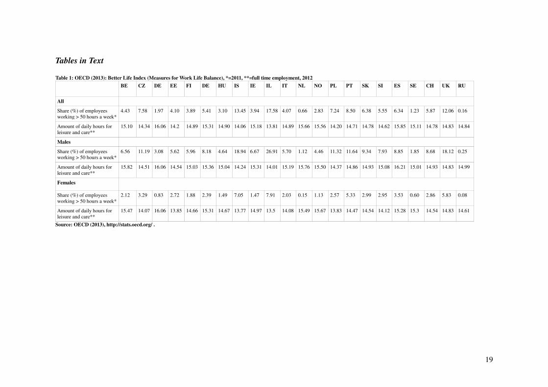
In table 1 I start with cross-country findings from the Organisation for Economic Co-

operation and Development (OECD 2013) for two factors which effect individual WLB.

One one hand a substantial part of a countries' labor force works more than 50 hours per

week. One the other hand men and women have around 14 to 15 hours a day for private

1See Drobnič et al. (2010), Hauret and Williams (2013), or Humpert (2010, 2014b) for analyzes of life

and job satisfaction in several European countries with transnational survey data.

2 I use the data version 1.2 with corrected values for Hungary.

4

purpose activities, such as leisure time or care.

Table 1 here

The key finding of the paper is that males and females suffer differently from working

time mismatch. Males LS and JS is not effected by over-time, while females react with

dissatisfaction. Analyzing WLB direct shows that males and females suffer from a shift

from leisure time towards working time. However, females are more sensitive. This can

be explained by the multiple burdens of paid work and household production, especially

by caring children.

The paper is structured like that. After this introduction, I give a literature review (2),

and discuss the data and the used methods are described in section 3. In section 4 and 5

the results are presented and discussed.

2. References from the Literature

Booth and van Ours (2008) show in an influential paper that British partnered men and

women behave different in terms of working hours and JS. In general women report

lower levels of JS. The authors use the BHPS panel data and present clear evidence, that

male JS or LS are not affected by the size of hours worked, while their satisfaction with

working hours is the highest at full time work level respectively 40 hours per week.

Nevertheless, over-time work is dissatisfying. Women, however have their highest level

of JS and satisfaction with working hours at the part time level. The results for women

5

lead to the hypotheses that they should prefer part time work, but LS as a whole remain

not affected. In a similar paper Booth and van Ours (2013) replicate these results with

Dutch data. Here women working part-time report their highest levels of JS.

With Australian Hilda panel data Wooden et al. (2009) analyze the effects of working

time mismatch on JS. They present two key findings: at first not the number of hours

worked, but any mismatch between preferred and realized hours lower JS. Second, they

show that both, working more or working fewer hours than contractual fixed are

dissatisfying, as well. However, the effect of working over-time is the larger one.

Wunder and Heineck (2013) use German SOEP panel data to show that working time

mismatch reduces LS. Women with full-time working husbands report their highest

satisfaction with life, while males remain not effected of their wife´s provided working

hours. Contrary to other studies, they present clear evidence that under-time harms more

than over-time. While occupational sex segregation declines in Germany on the long-

run, Humpert (2014a) shows that segregation remains higher in the former socialistic

part of Eastern Germany. Although, this finding is observable for full-time and part-time

work, segregation is always lower in part-time employment.

Using U.S. data, Tausig and Fenwick (2001) discuss several variables who affect an

individual’s WLB. While working over-time or working at the weekend reduces the

WLB, union membership increases it. A somehow surprising result is, that there exist no

gender specific differences, while the presence of young children reduces the WLB in

general.

6

Pereira and Coelho (2013) show with pooled ESS data3 that interruption in carrier, such

as times of former unemployment lower job satisfaction. But is there is evidence, that

autonomy in the daily working routing, a large firm size and a non-fixed working

contract will increase job satisfaction.

Hofäcker and König (2013) use the 2010 ESS wave and analyze three psychological

measures on WLB4. Although, only a few country groups have significant coefficients,

the authors show that in Scandinavian and Anglo-Saxon countries people report the

lowest conflicts between working and leisure time.

In this context health is an important factor. In review articles Sparks et al. (1997), and

Bassanini and Caroli (2014) analyze the nexus between working time and physical or

mental health. They show a non-linear relation between these two characteristics.

Working more or less hours than expected has both negative effects, especially

psychological. An important factor in coping with under- or over-time is a personal

influence in making decision.

However productivity effects on the firm level, provide only mixed evidences. While

Konrad and Mangel (2000) show higher productivity of firm, who provide WLB

methods to the employees, Bloom et al (2009) show no effect. Here controlling for

management stile turns the coefficients from positive to zero.

3 Here, the 2002, 2004, and 2006 waves of the ESS data were pooled as one data set.

4 The information on satisfaction with WLB was used in earlier waves, e.g. by Ylikännö (2010) for four

Scandinavian countries.

7

3. Data and Empirical Model

I use the recently published 2012 wave of the European Social Survey (ESS 2012), an

international social-economic cross-section data set. The data includes 44,257

individuals from 24 industrialized countries5. For my analysis I only exclude the

Kosovo6 which is neither a member states of the EU nor the OECD, and limit the data

to 12,759 employed individuals (6,329 men and 6,430 women) on an age range between

18 and 65 years. There are three similar questions on individual LS, JS, and WLB. The

questions are the following:

“All things considered, how satisfied are you with your life as a whole nowadays?”

“All things considered, how satisfied are you with your present job?7”

“How satisfied are you with the balance between the time you spend on your paid work

and the time you spend on other aspects of your life?”

They had to be answered on a typical Likert-skale from 0 to 10, where 0 means

extremely dissatisfied and 10 extremely satisfied. For the dependent variable I collapse

the scales from 0 to 10 into binary scales. This information is grouped at their means.

Therefore the dummies turn to zero when satisfaction is reported from 0 to 7 (not

satisfied), and into one (satisfied) for values between 8 to 10. Recoding the longer scale

into a binary variable is a usual procedure. This is used e.g. in earlier papers by

Kassenboehmer and Haisken-DeNew (2009), Hauret and Williams (2013), or Humpert

5 These countries are Belgium, Bulgaria, Cyprus, Czech Republic, Denmark, Estonia, Finland, Germany,

Hungary, Iceland, Ireland, Israel, Kosovo, Netherlands, Norway, Poland, Portugal, Russian Federation,

Slovakia, Slovenia, Spain, Sweden, Switzerland and United Kingdom.

6 The Russian Federation was invited by the OECD to participate in 2007.

7 If respondents have several jobs, they should answer about the main one.

8

(2013).

The main independent variables are working time specific. At first, I use the coding

presented by Booth and van Ours (2008) and recode the working hours inclusive paid

and unpaid over-time into four dummy variables. These are the following: small part-

time (1 to 15 hours per week), large part-time (16 to 29 hours), full-time (30 to 40

hours), and over-time (more than 40 hours). This assumption is appropriate, because on

average males in the sample work around 42 hours a week and females around 38 hours.

However, it is obvious that especially males are underrepresented in the group less than

15 hours per week. See table 2 for the distribution of working hours per country and

gender.

Table 2 here

At second, I compute new dummy variables for the difference between regular working

hours and contractual working hours. This allows information on more or less worked

hours. The reference group is having no calculated differences. For robustness reasons I

use the same information as the numeric difference. The other controls are related to

social-economic and employment specific conditions. The social-economic controls are

age, age squared, education level, having children, having a partner and citizenship of

the individual country observed. The employment related controls are fixed contract,

having influence on daily work, supervision of employees, working in public sector,

union membership, ever been unemployment and household income from work.

Country specific dummies control for macroeconomic differences. These are not

9

discussed. The descriptive statistics separated for males and females are presented in

table 3.

Table 3 here

I perform binary probit estimations with marginal effects. These are the percentage

changes when a dummy turns from zero to one, while all other variables are hold

constant. Following the data set description by ESS (2012) the use of design weights is

obligatory. The general estimation equation is the following:

satisfactioni = a0+a1 working timei +Xi b+εi (1)

For every individual i the LS or JS, or satisfaction with WLB are regressed on a set of

dummy variables on working time regimes, or on over- and under-time (a1 working

timei) and a vector of individual social-economic and employment specific

characteristics Xi b. Epsilon (εi) presents the residuum.

4. Results

As expected men and women differ in terms of LS, JS, WLB, and working hours.

At first, there are rather no effects for males on any satisfaction. The results are

presented in table 4. There is weak evidence that male LS is effected by working hours.

While working more than 40 hours a week increases LS positive with 10 percent,

neither dummies for over- or under-time nor the number of additional hours have any

10

statistical effect. This is similar to the results for JS. Again, males are not affected by

any differences in working hours. However, the results change for WLB. Here working

more than 40 hours a week lowers WLB with -14 percent. The regression with dummies

for over- and under-time show similar results with -12,5 percent for over-time. The

reference is a dummy for no calculated difference between actual and contractual

working hours. At third, a change in the number of working hours lowers WLB with -1

percent. All these coefficients are significant at the 1 percent level.

All other controls show results in line with the literature findings. While LS and JS have

a u-shaped age profile, WLB do not differ with age. The size of household income is

always positive for any satisfaction or WLB. While dummies for private sector

employment and especially control on own work routines increase any satisfaction or

WLB, past unemployment decrease it. Having a leading position at the work place

affects only JS positive.

Table 4 here

The results for women differ towards the male results above. While the three dummies

for working hour groups provide no results, dummies for under- and over-time both

show negative effects on LS. Here, doing fewer hours on the labor market lowers LS

with 10 percent, while doing more hours lowers it with 4 percent. Again numeric

differences in working hours provide no statistical evidence. The results for JS show

much clearer effects. Working 30 to 40 hours or more than 40 hours a week lower

female JS with -7, respectively -10 percent. Doing under- or over-time provide similar

results. Relative to the no calculated differences, over-time lowers JS with -3 percent.

11

Again, change in the number of working hours has no statistical effect.

Female WLB is more sensitive to working time differences than male WLB. Here,

dummies for working 30 to 40 hours lower WLB with -19 percent. Doing more than 40

hours a week is even more negative with -30 percent. Dummies for under- and over-

time are both negative effected, relative to no difference. Doing less hours lowers WLB

with -8 percent, while doing more hours lowers it with -14 percent. Similar to male

WLB, a change in the number of working hours lowers WLB by -1 percent.

Again, the controls show the expected results. While LS and JS have a u-shaped age

profile, WLB do not differ with age. The size of household income is positive for any

satisfaction or WLB. Private sector employment affects LS and JS, but no WLB.

Having control to own work routines has a highly significant positive effect, while past

unemployment decrease any type of satisfaction or WLB. Women are slightly negative

affected by children in the household in terms of LS and WLB, but not of JS. A leading

position at the work place has even mixed results for women. It increases JS, but lowers

WLB.

Table 5 here

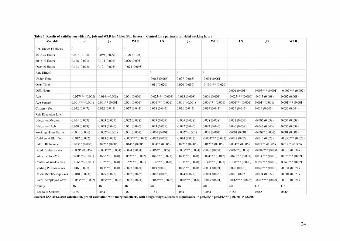
In the next step I repeat the analysis with a smaller sub sample. I substitute the dummy

variable of being partnered or not, towards the number of working hours of an

individual's partner. This is closer to the idea described by Booth and van Ours (2008,

2013), and Wunder and Heineck (2013). However, the number of observation is lowered

to the half, because single households and non-employed partners are dropped. Now

12

6,915 observations remain, with 3,406 men and 3,509 women. While the (female)

partners of males provide 35.6 working hours a week to the labor market on the

average, (male) partners of females work with 42.1 hours much longer.8

Table 6 and 7

show the estimation results, separately for men and women.

The male results are quite similar to those of table 4. None of the three types of working

hours are affected by LS. This is similar to the results for JS. Neither the dummies for

working hours, nor the dummies for under- or over-time are affected. However, by

using the calculated difference in the numbers of hours shows a positive and highly

significant result. Here, a change in the number of working hours increases JS by 1

percent. Once again, males’ results slightly change for WLB. Although, dummies for

working hours are not affected, the dummy for over-time turns towards -13 percent. At

third, a change in the number of working hours lowers WLB with -1 percent. As

reported in the earlier section, all other controls for males show results in line with the

literature findings.

Table 6 here

The female results for the restricted sample in table 6 are similar to the earlier one.

While the three dummies for working hour groups provide no results, dummies for

under- and over-time both show negative effects on LS. Here, doing fewer hours on the

labor market lowers LS with 10 percent, while doing more hours lowers it with 4

percent. Again numeric differences in working hours provide no statistical evidence.

8 There is no identification of a partner's gender type. So I assume that the most of the couples in the data

should be heterosexual men and women.

13

The results for JS show much clearer effects. Working 30 to 40 hours or more than 40

hours a week lower female JS with -8, respectively -12 percent. Doing less working

hours lowers JS by -15 percent, while working more remains at a level of -4 percent. A

numeric change in the number of working hours has no effect.

The results for female WLB are even larger and more sensitive to working time

differences than in table 5. Here, dummies for working 30 to 40 hours lower WLB by -

22 percent. Doing more than 40 hours a week is even more negative with -35 percent.

Dummies for under- and over-time are both negative effected, relative to no difference.

Doing fewer hours lowers WLB with -10 percent, while doing more hours lowers it

with -15 percent. Again a change in the number of working hours lowers WLB with -1

percent. Again the controls support the findings discussed above.

Table 7 here

5. Conclusion and Limitations

In the estimation presented above I use different measures of satisfaction and WLB to

analyze if and how an individual's life is affected by working more or less hours than

preferred. The key finding of the paper is that males and females suffer differently from

any working time mismatch.

In terms of LS, and JS males are slightly uninfected by working shorter or longer than

contractual fixed. However, the WLB measure shows that males suffer from over-time,

because of the loss in leisure time. Women seem to be more sensitive towards

14

differences in working hours. Here LS is both negative effected by under- and over-

time. However, effects of working fewer hours are even larger. The results for JS and

WLB show that women seem to prefer part-time employment. Relative to working

small part-time, full-time and doing over-time both lower JS significantly. The results

for WLB regressions are larger each time. By using direct dummies for working extra or

less hours, under-time has larger negative effects in estimations of JS, but lowers in

estimations of WLB. The results for females may be explained by a multiple burden of

paid work and household production, especially by raising and caring children. This

finding is supported by lowering effects of carrier variables, such as having a leading

position.

However, there are some limitations of the study. At first, I am only able to use cross-

section and cross-country information. Therefore, any answers towards question of

causality are difficult to answer. Second, because of limited numbers of observation per

country, I can only use the cross-country information as a control. The use of country

specific data may foster the presented result. However, the overall effects are in line

with the literature findings on LS, JS, and WLB.

Acknowledgment

This paper is the private opinion of the author and not of his institutions.

15

Literature

Bassanini, A. and Caroli, E., 2014. Is work bad for health? The role of constraint vs

choice, IZA Discussion Paper 7891.

Bloom, N., Kretschmer, T. and Van Reenan, J., 2009. Work-life balance, management

practices and productivity, in: international differences in the business practices and

productivity of firms, Freeman, R. and Shaw, K. L.(Eds.), University of Chicago Press,

15-54.

Booth, A.I. and van Ours, J.C., 2008. Job satisfaction and family happiness: The part-

time work puzzle, The Economic Journal 118, F77-F99.

Booth, A.I. And van Ours, J.C., 2013. Part-time jobs: what women want?, Journal of

Population Economics, 26 (1), 263-283.

Bulger, C., 2014. Work life balance, in: Encyclopedia of Quality of Life and Well-Being

Research, Michalos, A. C. (Ed.), Springer Heidelberg, 7231-7232.

Drobnič, S., Beham, B. and Präg, P., 2010. Good life, good job? Working conditions and

quality of life in Europe, Social Indicator Research, 99 (2), 205-225.

ESS Round 6: European Social Survey Round 6 Data, 2012. Data file edition 1.2.

Norwegian Social Science Data Services, Norway – Data Archive and distributor of

16

ESS data.

Guest, D.E., 2002. Perspectives on the study of work-life balance, Social Science

Information, 41 (2), 255-279.

Hauret, L. and Williams, D. R.,2013. Cross-national analysis of gender differences in

job-satisfaction, CEPS Instead working paper 2013-27.

Hofäcker, D. and König, S., 2013. Flexibility and work-life conflict in times of crisis: A

gender perspective, International Journal of Sociology and Social Policy, 33 (9/10), 613-

635.

Humpert, S., 2010. A note on happiness in Eastern Europe, European Research Studies,

13 (3), 133-144.

Humpert, S., 2013. Gender differences and social participation, International Journal of

Economic Sciences and Applied Research, 6 (3), 123-142.

Humpert, S., 2014a. Occupational sex segregation and working time: Regional evidence

from Germany, Panoeconomicus,61 (3), 317-329.

Humpert, S., 2014b. Well-being, work and government: Insights from Eastern transition

countries, Pecob's Papers Series, No.41.

17

Konrad, A.M. And Mangel, R., 2000. The impact of work-life programs on firm

productivity, Strategic Management Journal, 21 (12), 1225-1237.

Lewis, S., Gambles, R. and Rapoport, R., 2007. The constraints of a 'work-life balance'

approach: An international perspective, The International Journal of Human Resource

Management, 18 (3), 360-373.

OECD, 2013. How's life? 2013: Measuring well-being, OECD Publishing, 50-52.

Pereira, M.C. and Coelho, F., 2013. Work hours and well being: An investigation of

moderator effects, Social Indicator Research 111(1), 235-253.

Sparks, K., Cooper, C., Fried Y., and Shirmon, A., 1997. The effects of hours worked on

health: A meta-analytic review, Journal of Occupational and Organizational Psychology,

70 (4), 391-408.

Tausig, M. and Fenwick, R., 2001. Unbinding time: Alternate work schemes and work

life balance, Journal of Family and Economic Issues, 22 (2), 101-119.

Wooden, M., Warren, D. and Drago, R., 2009. Working time mismatch and subjective

well-being, British Journal of Industrial Relations, 47 (1), 147-179.

Wunder, C. and Heineck, G., 2013. Working time preferences, hours mismatch and

well-being of couples: Are there spillovers?, Labor Economics, 27 (October), 244-252.

18

Ylikännö, M., 2010. Employees' satisfaction with the balance between work and leisure

in Finland, Sweden, Norway and Denmark – Time use perspective, Research on Finnish

Studies, 3 , 43-52.

19

Tables in Text

Table 1: OECD (2013): Better Life Index (Measures for Work Life Balance), *=2011, **=full time employment, 2012

BE

CZ DE EE FI DE HU IS IE IL IT NL NO PL PT SK SI ES SE CH UK RU

All

Share (%) of employees

working > 50 hours a week*

4.43 7.58 1.97 4.10 3.89 5.41 3.10 13.45 3.94 17.58 4.07 0.66 2.83 7.24 8.50 6.38 5.55 6.34 1.23 5.87 12.06 0.16

Amount of daily hours for

leisure and care**

15.10 14.34 16.06 14.2 14.89 15.31 14.90 14.06 15.18 13.81 14.89 15.66 15.56 14.20 14.71 14.78 14.62 15.85 15.11 14.78 14.83 14.84

Males



6.56

11.19 3.08 5.62 5.96 8.18 4.64 18.94 6.67 26.91 5.70 1.12 4.46 11.32 11.64 9.34 7.93 8.85 1.85 8.68 18.12 0.25


leisure and care**

15.82 14.51 16.06 14.54 15.03 15.36 15.04 14.24 15.31 14.01 15.19 15.76 15.50 14.37 14.86 14.93 15.08 16.21 15.01 14.93 14.83 14.99

Females



2.12

3.29 0.83 2.72 1.88 2.39 1.49 7.05 1.47 7.91 2.03 0.15 1.13 2.57 5.33 2.99 2.95 3.53 0.60 2.86 5.83 0.08


leisure and care**

15.47 14.07 16.06 13.85 14.66 15.31 14.67 13.77 14.97 13.5 14.08 15.49 15.67 13.83 14.47 14.54 14.12 15.28 15.3 14.54 14.83 14.61

Source: OECD (2013), http://stats.oecd.org/ .

20

Table 2: Means working hours by country and gender

Country All: Mean

(Std. Dev.)

Males: Mean

(Std. Dev.)

Females: Mean

(Std. Dev.)

BE 38.14 (0.421) 41.54 (0.581) 34.50 (0.544)

BG 42.56 (0.402) 43.77 (0.584) 41.32 (0.540)

CH 41.52 (0.463) 42.48 (0.734) 40.48 (0.533)

CY 40.41 (0.284) 42.40 (0.355) 38.44 (0.420)

CZ 42.22 (0.373) 44.15 (0.597) 40.98 (0.467)

DE 38.23 (0.556) 39.01 (0.827) 37.69 (0.746)

DK 43.85 (0.443) 46.67 (0.582) 40.52 (0.613)

EE 39.22 (0.330) 41.48 (0.434) 36.43 (0.470)

ES 35.52 (0.412) 49.23 (0.452) 30.39 (0.587)

FI 42.74 (0.849) 48.10 (1.175) 37.91 (1.059)

GB 41.03 (0.665) 48.09 (0.954) 35.73 (0.764)

HU 37.21 (0.510) 40.42 (0.628) 34.46 (0.736)

IE 41.20 (0.295) 42.14 (0.402) 40.37 (0.420)

IL 37.61 (0.509) 42.61 (0.701) 33.91 (0.653)

IS 38.99 (0.235) 40.53 (0.330) 37.33 (0.317)

NL 40.73 (0.457) 43.40 (0.552) 37.74 (0.697)

NO 42.38 (0.329) 44.32 (0.522) 40.77 (0.403)

PL 37.80 (0.3439 39.99 (0.503) 35.44 (0.428)

PT 39.61 (0.347) 43.36 (0.396) 35.04 (0.533)

RU 43.89 (0.264) 44.40 (0.359) 43.26 (0.386)

SE 40.35 (0.689) 42.46 (1.047) 38.38 (0.867)

SI 38.96 (0.467) 43.90 (0.473) 32.89 (0.711)

SK 42.06 (0.282) 42.99 (.462) 41.35 (0.347)

Sample Mean 40.07 (0.087) 42.79 (0.1169 37.39 (0.123) Source: ESS 2012, own calculation, with design weights.

21

Table 3: Description Statistics

Males Females

Variable Obs. Mean Std. Dev. Min. Max. Obs. Mean Std. Dev. Min. Max.

LS 6,329 0.567 0.495 0 1 6,430 0.560 0.497 0 1

JS 6,329 0.594 0.491 0 1 6,430 0.590 0.492 0 1

WLB 6,329 0.419 0.493 0 1 6,430 0.418 0.493 0 1

15 to 29 Hours 6,329 0.031 0.174 0 1 6,430 0.132 0.338 0 1

30 to 40 Hours 6,329 0.477 0.499 0 1 6,430 0.566 0.496 0 1

Over 40 Hours 6,329 0.479 0.500 0 1 6,430 0.266 0.442 0 1

Under-Time 6,329 0.021 0.145 0 1 6,430 0.021 0.144 0 1

Over-Time 6,329 0.464 0.498 0 1 6,430 0.353 0.478 0 1

Diff. Hours 6,329 3.599 7.039 -45 75 6,430 2.216 5.440 -40 48

Age 6,329 42.107 11.618 18 65 6,430 42.707 11.322 18 65

Age Square 6,329 1,907.959 983.471 324 4,225 6,430 1,952.073 966.527 324 4,225

Citizen 6,329 0.945 0.228 0 1 6,430 0.959 0.196 0 1

Education Medium 6,329 0.521 0.500 0 1 6,430 0.432 0.495 0 1

Education High 6,329 0.389 0.488 0 1 6,430 0.481 0.499 0 1

Partner at HH 6,329 0.716 0.451 0 1 6,430 0.651 0.476 0 1

Children at HH 6,329 0.488 0.500 0 1 6,430 0.542 0.498 0 1

Index HH Income 6,329 6.654 2.418 1 10 6,430 6.269 2.537 1 10

Fixed Contract 6,329 0.121 0.327 0 1 6,430 0.136 0.343 0 1

Public Sector 6,329 0.283 0.450 0 1 6,430 0.461 0.498 0 1

Control of Work 6,329 0.523 0.499 0 1 6,430 0.513 0.499 0 1

Leading Position 6,329 0.370 0.483 0 1 6,430 0.260 0.439 0 1

Union Membership 6,329 0.359 0.480 0 1 6,430 0.377 0.485 0 1

Ever Unemployed 6,329 0.299 0.455 0 1 6,430 0.279 0.449 0 1 Source: ESS 2012, own calculation, with design weights.

22

Table 4: Results of Satisfaction with Life, Job and WLB for Males (Std. Errors)

Variable LS JS WLB LS JS WLB LS JS WLB

Ref. Under 15 Hours / / /

15 to 29 Hours -0.011 (0.072) 0.006 (0.069) 0.035 (0.071)

30 to 40 Hours 0.097 (0.611) 0.086 (0.060) -0.004 (0.060)

Over 40 Hours 0.101* (0.614) 0.096 (0.060) -0.142*** (0.06)

Ref. Diff.=0 / / /

Under-Time -0.025 (0.051) 0.029 (0.047) 0.070 (0.048)

Over-Time -0.006 (0.015) 0.005 (0.015) -0.125*** (0.014)

Diff. Hours -0.001 (0.001) -0.001 (0.001) -0.008*** (0.001)

Age -0.024*** (0.005) -0.014*** (0.005) -0.006 (0.004) -0.022*** (0.005) -0.012*** (0.005) -0.007 (0.005) -0.022*** (0.005) -0.012*** (0.005) -0.008 (0.005)

Age Square 0.001*** (0.001) 0.001*** (0.001) 0.001** (0.001) 0.001*** (0.001) 0.001*** (0.001) 0.001** (0.001) 0.001** (0.001) 0.001*** (0.001) 0.001*** (0.001)

Citizen =Yes 0.042 (0.032) 0.036 (0.031) 0.030 (0.029) 0.043 (0.032) 0.036 (0.030) 0.035 (0.030) 0.042 (0.032) 0.037 (0.030) 0.035 (0.029)

Ref: Education Low

Education Medium 0.012 (0.026) -0.007 (0.025) -0.016 (0.025) 0.011 (0.026) -0.008 (0.025) -0.010 (0.025) 0.011 (0.026) -0.008 (0.025) -0.016 (0.025)

Education High 0.035 (0.026) -0.028 (0.027) -0.023 (0.027) 0.034 (0.027) -0.029 (0.027) -0.007 (0.027) 0.033 (0.027) -0.030 (0.027) -0.020 (0.026)

Partner at HH =Yes 0.132*** (0.019) 0.001 (0.018) 0.008 (0.018) 0.132*** (0.020) 0.001 (0.018) 0.006 (0.018) 0.131*** (0.020) 0.001 (0.018) 0.003 (0.018)

Children at HH =Yes -0.016 (0.178) -0.005 (0.017) -0.031** (0.017) -0.017 (0.018) -0.005 (0.017) -0.030** (0.017) -0.017 (0.018) -0.006 (0.017) -0.031** (0.017)

Index HH Income 0.034*** (0.004) 0.023*** (0.003) 0.016*** (0.003) 0.035*** (0.004) 0.024*** (0.003) 0.014*** (0.003) 0.035*** (0.003) 0.024*** (0.003) 0.014*** (0.003)

Fixed Contract =Yes -0.001 (0.023) 0.001 (0.021) -0.014 (0.021) -0.002 (0.023) 0.001 (0.021) -0.012 (0.021) -0.002 (0.023) -0.002 (0.033) -0.011 (0.021)

Public Sector=Yes 0.038*** (0.016) 0.069*** (0.015) 0.065*** (0.016) 0.034*** (0.016) 0.065*** (0.015) 0.071*** (0.016) 0.034*** (0.016) 0.065*** (0.015) 0.071*** (0.016)

Control of Work = Yes 0.123*** (0.015) 0.212*** (0.015) 0.156*** (0.015) 0.123*** (0.015) 0.212*** (0.014) 0.152*** (0.015) 0.123*** (0.015) 0.212*** (0.015) 0.151*** (0.015)

Leading Position =Yes 0.007 (0.016) 0.037*** (0.015) -0.020 (0.015) 0.011 (0.016) 0.039*** (0.015) -0.026* (0.015) 0.010 (0.016) 0.040*** (0.015) -0.027* (0.015)

Union Membership =Yes -0.028* (0.017) -0.007 (0.017) 0.011 (0.017) -0.027 (0.017) -0.005 (0.017) 0.013 (0.017) -0.027 (0.018) -0.005 (0.017) 0.013 (0.017)

Ever Unemployed =Yes -0.077*** (0.016) -0.061*** (0.015) -0.041*** (0.015) -0.079*** (0.016) -0.062*** (0.015) -0.037*** (0.015) -0.079*** (0.016) -0.062*** (0.015) -0.039*** (0.015)

County OK OK OK OK OK OK OK OK OK

Pseudo R-Squared 0.182 0.092 0.061 0.181 0.091 0.059 0.181 0.091 0.059 Source: ESS 2012, own calculation, probit estimation with marginal effects, with design weights, levels of significance: * p<0.05,** p<0.01,*** p<0.001, N=6,329.

23

Table 5: Results of Satisfaction with Life, Job and WLB for Females (Std. Errors)



15 to 29 Hours 0.065 (0.041) -0.002 (0.039) -0.003 (0.037)

30 to 40 Hours -0.006 (0.039) -0.069** (0.037) -0.188*** (0.036)

Over 40 Hours -0.015 (0.040) -0.095*** (0.039) -0.305*** (0.031)

Ref. Diff.=0 / / /

Under-Time -0.096** (0.052) -0.042 (0.052) -0.084* (0.044)

Over-Time -0.036*** (0.016) -0.025* (0.015) -0.143*** (0.015)

Diff. Hours -0.001 (0.001) -0.001 (0.001) -0.012*** (0.002)

Age -0.019*** (0.005) -0.015*** (0.005) -0.006 (0.005) -0.019*** (0.005) -0.016*** (0.005) -0.010*** (0.005) -0.019*** (0.005) -0.016*** (0.005) -0.011*** (0.005)

Age Square 0.001*** (0.001) 0.001*** (0.001) 0.001*(0.001) 0.001*** (0.001) 0.001*** (0.001) 0.001*** (0.001) 0.001*** (0.001) 0.001*** (0.001) 0.001*** (0.001)

Citizen =Yes 0.058 (0.037) 0.073*** (0.036) 0.047 (0.033) 0.060* (0.037) 0.077*** (0.036) 0.059* (0.033) 0.059 (0.037) 0.076*** (0.035) 0.054 (0.033)

Ref: Education Low

Education Medium 0.023 (0.028) -0.015 (0.025) 0.030 (0.026) 0.020 (0.028) -0.019 (0.025) 0.017 (0.026) 0.022 (0.028) -0.018 (0.026) 0.018 (0.026)

Education High 0.059*** (0.029) 0.001 (0.027) 0.014 (0..027) 0.059*** (0.029) -0.004 (0.027) 0.002 (0.027) 0.057** (0.029) -0.006 (0.027) -0.001 (0.027)

Partner at HH =Yes 0.081*** (0.017) -0.016 (0.016) -0.026 (0.016) 0.083*** (0.017) -0.013 (0.016) -0.015 (0.016) 0.085*** (0.017) -0.012 (0.016) -0.010 (0.016)

Children at HH =Yes -0.032** (0.017) 0.009 (0.016) -0.034*** (0.003) -0.026 (0.017) 0.017 (0.016) -0.008 (0.016) -0.025 (0.017) 0.017 (0.016) -0.008 (0.015)

Index HH Income 0.027*** (0.004) 0.015*** (0.003) 0.008*** (0.003) 0.027*** (0.004) 0.014*** (0.003) 0.006*** (0.003) 0.026*** (0.003) 0.014*** (0.003) 0.006* (0.003)

Fixed Contract =Yes -0.032 (0.023) 0.001 (0.020) 0.016 (0.020) -0.029 (0.022) 0.005 (0.020) 0.027 (0.021) -0.028 (0.022) 0.005 (0.020) 0.029 (0.020)

Public Sector=Yes 0.027* (0.016) 0.041*** (0.015) 0.007 (0.014) 0.029* (0.016) 0.042*** (0.015) 0.014 (0.015) 0.029** (0.015) 0.042*** (0.014) 0.014 (0.015)


Leading Position =Yes 0.007 (0.018) 0.032** (0.017) -0.033*** (0.016) 0.006 (0.017) 0.026 (0.016) -0.051*** (0.016) 0.001 (0.017) 0.023 (0.016) -0.059 (0.016)

Union Membership =Yes -0.032* (0.018) 0.004 (0.017) 0.003 (0.017) -0.034* (0.018) 0.001 (0.018) -0.007 (0.017) -0.034**(0.018) 0.001 (0.018) -0.002 (0.017)

Ever Unemployed =Yes -0.059*** (0.017) -0.048*** (0.016) -0.038*** (0.015) -0.057*** (0.016) -0.047*** (0.016) -0.034*** (0.015) -0.058*** (0.017) -0.047*** (0.016) -0.034*** (0.015



24

Table 6: Results of Satisfaction with Life, Job and WLB for Males (Std. Errors) : Control for a partner's provided working hours



15 to 29 Hours 0.007 (0.105) 0.059 (0.099) 0.170 (0.105)

30 to 40 Hours 0.128 (0.091) 0.104 (0.092) 0.090 (0.095)

Over 40 Hours 0.143 (0.093) 0.121 (0.093) -0.074 (0.095)

Ref. Diff.=0 / / /

Under-Time -0.068 (0.066) 0.027 (0.063) -0.001 (0.061)

Over-Time 0.011 (0.020) 0.020 (0.019) -0.130*** (0.020)

Diff. Hours 0.001 (0.001) 0.003*** (0.001) -0.009*** (0.002)

Age -0.027*** (0.008) -0.014* (0.008) 0.001 (0.001) -0.025*** (0.008) -0.013 (0.008) 0.001 (0.001) -0.025*** (0.009) -0.013 (0.008) 0.002 (0.008)

Age Square 0.001*** (0.001) 0.001** (0.001) 0.001 (0.001) 0.001*** (0.001) 0.001* (0.001) 0.001*** (0.001) 0.001*** (0.001) 0.001* (0.001) 0.001*** (0.001)

Citizen =Yes 0.032 (0.047) 0.022 (0.045) 0.027 (0.044) 0.028 (0.047) 0.021 (0.045) 0.039 (0.044) 0.029 (0.047) 0.019 (0.045) 0.036 (0.044)

Ref: Education Low

Education Medium 0.034 (0.037) -0.003 (0.037) 0.032 (0.038) 0.029 (0.037) -0.005 (0.038) 0.038 (0.038) 0.031 (0.037) -0.006 (0.038) 0.034 (0.038)

Education High 0.050 (0.039) -0.038 (0.040) 0.031 (0.040) 0.043 (0.039) -0.042 (0.040) 0.047 (0.040) 0.046 (0.039) -0.043 (0.040) 0.036 (0.039)

Working Hours Partner -0.001 (0.001) -0.002* (0.001) 0.001 (0.001) -0.001 (0.001) -0.002* (0.001) 0.001 (0.001) -0.001 (0.001) -0.002* (0.001) 0.001 (0.001)

Children at HH =Yes -0.012 (0.022) -0.013 (0.022) -0.057*** (0.022) -0.012 (0.022) -0.014 (0.022) -0.054*** (0.022) -0.012 (0.022) -0.013 (0.022) -0.055*** (0.022)

Index HH Income 0.033** (0.005) 0.022** (0.005) 0.014** (0.005) 0.034** (0.005) 0.022** (0.005) 0.012** (0.005) 0.034** (0.005) 0.022** (0.005) 0.012** (0.005)

Fixed Contract =Yes -0.059* (0.035) -0.083*** (0.034) -0.024 (0.034) -0.063* (0.035) -0.085*** (0.034) -0.020 (0.034) -0.063* (0.035) -0.087*** (0.034) -0.015 (0.034)

Public Sector=Yes 0.050*** (0.021) 0.075*** (0.020) 0.067*** (0.022) 0.046*** (0.021) 0.073*** (0.020) 0.074*** (0.012) 0.046*** (0.021) 0.074*** (0.020) 0.076*** (0.021)


Leading Position =Yes 0.016 (0.021) 0.043*** (0.020) -0.023 (0.021) 0.019 (0.020) 0.045*** (0.020) -0.031 (0.021) 0.020 (0.020) 0.042*** (0.020) -0.031 (0.021)

Union Membership =Yes -0.018 (0.023) -0.025 (0.022) -0.002 (0.023) -0.018 (0.023) -0.024 (0.022) -0.001 (0.023) -0.018 (0.023) -0.024 (0.022) -0.001 (0.023)

Ever Unemployed =Yes -0.063*** (0.022) -0.045*** (0.021) -0.023 (0.021) -0.065*** (0.022) -0.046*** (0.020) -0.017 (0.021) -0.065*** (0.023) -0.045*** (0.021) -0.019 (0.021)



25

Table 7: Results of Satisfaction with Life, Job and WLB for Females (Std. Errors) : Control for a partner's provided working hours



15 to 29 Hours 0.057 (0.048) -0.022 (0.052) -0.049 (0.051)

30 to 40 Hours -0.011 (0.048) -0.080* (0.049) -0.220*** (0.048)

Over 40 Hours -0.015 (0.051) -0.123** (0.053) -0.350*** (0.040)

Ref. Diff.=0 / / /

Under-Time -0.105* (0.061) -0.148** (0.061) -0.103* (0.057)

Over-Time -0.039* (0.020) -0.043** (0.020) -0.149*** (0.019)

Diff. Hours -0.001 (0.001) -0.001 (0.001) -0.012*** (0.002)

Age -0.037*** (0.008) -0.011 (0.008) -0.008 (0.008) -0.037*** (0.008) -0.011 (0.008) -0.011 (0.008) -0.037*** (0.008) -0.011 (0.008) -0.011 (0.008)

Age Square 0.001*** (0.001) 0.001 (0.001) 0.001 (0.001) 0.001*** (0.001) 0.001 (0.001) 0.001* (0.001) 0.001*** (0.001) 0.001* (0.001) 0.001* (0.001)

Citizen =Yes 0.092* (0.050) 0.081* (0.047) 0.028 (0.045) 0.094** (0.049) 0.086* (0.047) 0.050 (0.045) 0.093* (0.049) 0.086* (0.047) 0.042 (0.045)

Ref: Education Low

Education Medium 0.068* (0.036) -0.011 (0.036) 0.067* (0.037) 0.068* (0.036) -0.014 (0.036) 0.060 (0.037) 0.069** (0.036) -0.012 (0.036) 0.064 (0.045)

Education High 0.106*** (0.038) 0.012 (0.038) 0.048 (0.038) 0.109*** (0.038) 0.008 (0.037) 0.041 (0.038) 0.107*** (0.038) 0.006 (0.037) 0.040 (0.038)

Working Hours Partner 0.001 (0.001) 0.001 (0.001) -0.001 (0.001) 0.001 (0.001) 0.001 (0.001) -0.001 (0.001) 0.001 (0.001) 0.001 (0.001) -0.002 (0.001)

Children at HH =Yes 0.019 (0.023) -0.001 (0.001) -0.043* (0.022) 0.025 (0.023) 0.010 (0.022) -0.011 (0.022) 0.025 (0.023) 0.011 (0.022) -0.012 (0.022)

Index HH Income 0.034** (0.005) 0.019** (0.005) 0.012** (0.005) 0.034** (0.005) 0.018** (0.005) 0.010** (0.005) 0.034** (0.005) 0.018*** (0.005) 0.008** (0.005)

Fixed Contract =Yes -0.063*** (0.030) 0.003 (0.027) 0.022 (0.029) -0.061** (0.030) 0.005 (0.027) 0.027 (0.029) -0.059** (0.030) 0.058 (0.280) 0.031 (0.028)

Public Sector=Yes -0.007 (0.021) 0.030 (0.019) -0.018 (0.019) -0.005 (0.020) 0.032* (0.019) -0.011 (0.020) -0.006 (0.021) 0.031 (0.019) -0.012 (0.020)

Control of Work = Yes 0.102*** (0.200) 0.225*** (0.019) 0.167*** (0.020) 0.102*** (0.200) 0.223*** (0.019) 0.158*** (0.020) 0.101*** (0.199) 0.222*** (0.019) 0.156*** (0.019

Leading Position =Yes -0.024 (0.023) -0.025 (0.021) -0.054*** (0.021) -0.024 (0.023) -0.021 (0.021) -0.071*** (0.021) -0.030 (0.023) 0.014 (0.021) -0.078*** (0.021)

Union Membership =Yes -0.039 (0.024) 0.002 (0.023) 0.010 (0.024) -0.042** (0.024) -0.001 (0.023) 0.010 (0.022) -0.041* (0.024) 0.010 (0.022) 0.007 (0.024)

Ever Unemployed =Yes -0.050*** (0.022) -0.037* (0.021) -0.025 (0.021) -0.049* (0.022) -0.036* (0.021) -0.020 (0.021) -0.050** (0.022) -0.037* (0.021) -0.021 (0.021)



Working Paper Series in Economics

(recent issues)

No.326: Arnd Kölling: Labor Demand and Unequal Payment: Does Wage Inequality matter? Analyzing the Influence of Intra-firm Wage Dispersion on Labor Demand with German Employer-Employee Data, November 2014

No.325: Horst Raff and Natalia Trofimenko: World Market Access of Emerging-Market Firms: The Role of Foreign Ownership and Access to External Finance, November 2014

No.324: Boris Hirsch, Michael Oberfichtner and Claus Schnabel: The levelling effect of product market competition on gender wage discrimination, September 2014

No.323: Jürgen Bitzer, Erkan Gören and Sanne Hiller: International Knowledge Spillovers: The Benefits from Employing Immigrants, November 2014

No.322: Michael Gold: Kosten eines Tarifabschlusses: Verschiedene Perspektiven der Bewertung, November 2014

No.321: Gesine Stephan und Sven Uthmann: Wann wird negative Reziprozität am Arbeitsplatz

akzeptiert? Eine quasi-experimentelle Untersuchung, November 2014

No.320: Lutz Bellmann, Hans-Dieter Gerner and Christian Hohendanner: Fixed-term contracts and dismissal protection. Evidence from a policy reform in Germany, November 2014

No.319: Knut Gerlach, Olaf Hübler und Wolfgang Meyer: Betriebliche Suche und Besetzung von Arbeitsplätzen für qualifizierte Tätigkeiten in Niedersachsen - Gibt es Defizite an geeigneten Bewerbern?, Oktober 2014

No.318: Sebastian Fischer, Inna Petrunyk, Christian Pfeifer and Anita Wiemer: Before-after differences in labor market outcomes for participants in medical rehabilitation in Germany, December 2014

No.317: Annika Pape und Thomas Wein: Der deutsche Taximarkt - das letzte (Kollektiv-) Monopol im Sturm der „neuen Zeit“, November 2014

No.316: Nils Braakmann and John Wildman: Reconsidering the impact of family size on labour supply: The twin-problems of the twin-birth instrument, November 2014

No.315: Markus Groth and Jörg Cortekar: Climate change adaptation strategies within the framework of the German “Energiewende” – Is there a need for government interventions and legal obligations?, November 2014

No.314: Ahmed Fayez Abdelgouad: Labor Law Reforms and Labor Market Performance in Egypt, October 2014

No.313: Joachim Wagner: Still different after all these years. Extensive and intensive margins of exports in East and West German manufacturing enterprises, October 2014

No.312: Joachim Wagner: A note on the granular nature of imports in German manufacturing industries, October 2014

No.311: Nikolai Hoberg and Stefan Baumgärtner: Value pluralism, trade-offs and efficiencies, October 2014

No.310: Joachim Wagner: Exports, R&D and Productivity: A test of the Bustos-model with enterprise data from France, Italy and Spain, October 2014

No.309: Thomas Wein: Preventing Margin Squeeze: An Unsolvable Puzzle for Competition Policy? The Case of the German Gasoline Market, September 2014

No.308: Joachim Wagner: Firm age and the margins of international trade: Comparable evidence from five European countries, September 2014

No.307: John P. Weche Gelübcke: Auslandskontrollierte Industrie- und Dienstleistungs-unternehmen in Niedersachsen: Performancedifferentiale und Dynamik in Krisenzeiten, August 2014

No.306: Joachim Wagner: New Data from Official Statistics for Imports and Exports of Goods by German Enterprises, August 2014

No.305: Joachim Wagner: A note on firm age and the margins of imports: First evidence from Germany, August 2014

No.304: Jessica Ingenillem, Joachim Merz and Stefan Baumgärtner: Determinants and interactions of sustainability and risk management of commercial cattle farmers in Namibia, July 2014

No.303: Joachim Wagner: A note on firm age and the margins of exports: First evidence from Germany, July 2014

No.302: Joachim Wagner: A note on quality of a firm’s exports and distance to destination countries: First evidence from Germany, July 2014

No.301: Ahmed Fayez Abdelgouad: Determinants of Using Fixed-term Contracts in the Egyptian Labor Market: Empirical Evidence from Manufacturing Firms Using World Bank Firm-Level Data for Egypt, July 2014

No.300: Annika Pape: Liability Rule Failures? Evidence from German Court Decisions, May 2014

No.299: Annika Pape: Law versus Economics? How should insurance intermediaries influence the insurance demand decision, June 2013

No.298: Joachim Wagner: Extensive Margins of Imports and Profitability: First Evidence for Manufacturing Enterprises in Germany, May 2014 [published in: Economics Bulletin 34 (2014), 3, 1669-1678]

No.297: Joachim Wagner: Is Export Diversification good for Profitability? First Evidence for Manufacturing Enterprises in Germany, March 2014 [published in: Applied Economics 46 (2014), 33, 4083-4090]

No.296: Joachim Wagner: Exports and Firm Profitability: Quality matters!, March 2014 [published in: Economics Bulletin 34 (2014), 3, 1644-1652]

No.295: Joachim Wagner: What makes a high-quality exporter? Evidence from Germany, March 2014 [published in: Economics Bulletin 34 (2014), 2, 865-874]

No.294: Joachim Wagner: Credit constraints and margins of import: First evidence for German manufacturing enterprises, February 2014 [published in: Applied Economics 47 (2015), 5, 415-430]

No.293: Dirk Oberschachtsiek: Waiting to start a business venture. Empirical evidence on the determinants., February 2014

No.292: Joachim Wagner: Low-productive exporters are high-quality exporters. Evidence from Germany, February 2014 [published in: Economics Bulletin 34 (2014), 2, 745-756]

No.291: Institut für Volkswirtschaftslehre: Forschungsbericht 2013, Januar 2014

(see www.leuphana.de/institute/ivwl/publikationen/working-papers.html for a complete list)

No.290: Stefan Baumgärtner, Moritz A. Drupp und Martin F. Quaas: Subsistence and substitutability in consumer preferences, December 2013

No.289: Dirk Oberschachtsiek: Human Capital Diversity and Entrepreneurship. Results from the regional individual skill dispersion nexus on self-employment activity., December 2013

No.288: Joachim Wagner and John P. Weche Gelübcke: Risk or Resilience? The Role of Trade Integration and Foreign Ownership for the Survival of German Enterprises during the Crisis 2008-2010, December 2013 published in: [Jahrbücher für Nationalökonomie und Statistik 234 (2014), 6, 758-774]

No.287: Joachim Wagner: Credit constraints and exports: A survey of empirical studies using firm level data, December 2013

No.286: Toufic M. El Masri: Competition through Cooperation? The Case of the German Postal Market, October 2013

No.285: Toufic M. El Masri: Are New German Postal Providers Successful? Empirical Evidence Based on Unique Survey Data, October 2013

No.284: Andree Ehlert, Dirk Oberschachtsiek, and Stefan Prawda: Cost Containment and Managed Care: Evidence from German Macro Data, October 2013

No.283: Joachim Wagner and John P. Weche Gelübcke: Credit Constraints, Foreign Ownership, and Foreign Takeovers in Germany, September 2013

No.282: Joachim Wagner: Extensive margins of imports in The Great Import Recovery in Germany, 2009/2010, September 2013 [published in: Economics Bulletin 33 (2013), 4, 2732-2743]

No.281: Stefan Baumgärtner, Alexandra M. Klein, Denise Thiel, and Klara Winkler: Ramsey discounting of ecosystem services, August 2013

No.280: Antonia Arsova and Deniz Dilan Karamen Örsal: Likelihood-based panel cointegration test in the presence of a linear time trend and cross-sectional dependence, August 2013

No.279: Thomas Huth: Georg von Charasoff’s Theory of Value, Capital and Prices of Production, June 2013

No.278: Yama Temouri and Joachim Wagner: Do outliers and unobserved heterogeneity explain the exporter productivity premium? Evidence from France, Germany and the United Kingdom, June 2013 [published in: Economics Bulletin, 33 (2013), 3, 1931-1940]

No.277: Horst Raff and Joachim Wagner: Foreign Ownership and the Extensive Margins of Exports: Evidence for Manufacturing Enterprises in Germany, June 2013

No.276: Stephan Humpert: Gender Differences in Life Satisfaction and Social Participation, May 2013

No.275: Sören Enkelmann and Markus Leibrecht: Political Expenditure Cycles and Election Outcomes Evidence from Disaggregation of Public Expenditures by Economic Functions, May 2013

No.274: Sören Enkelmann: Government Popularity and the Economy First Evidence from German Micro Data, May 2013

Leuphana Universität Lüneburg

Institut für Volkswirtschaftslehre

Postfach 2440

D-21314 Lüneburg

Tel.: ++49 4131 677 2321

email: [email protected]

www.leuphana.de/institute/ivwl/publikationen/working-papers.html

Date post:	03-Aug-2018
Category:	Documents
Upload:	vukien
View:	218 times
Download:	0 times

Working time, satisfaction and work life balance: A ... · Working time, satisfaction and work life...

Documents