C h a p t e r 4 : W o r k i n g w i t h t h e S o l o w G r o w t h M o d e l52
Figure 4.1 extends the Solow model from Figure 3.9 to consider two saving rates, s1 and s2, where s2 is greater than s1. Each saving rate determines a different curve for s • (y/k)—the one with s2 lies above that for s1. Re-call that the growth rate of capital per worker, �k/k, equals the vertical distance between the s • (y/k) curve and the horizontal line, s� � n. There are also two posi-tions for this horizontal line, one for s1 and the other for s2. However, this shift in the horizontal line turns out to be minor. Therefore, we can see from the Figure 4.1 that �k/k is higher at any capital per worker, k, when the saving rate is s2 rather than s1.
1 Specifi cally, at k(0), �k/k is higher when the saving rate is s2, rather than s1. (We have assumed that �k/k is greater than zero for both saving rates.)
For either saving rate, the growth rate of capital per worker, �k/k, declines as capital per worker, k, rises above k(0). When the saving rate is s1, �k/k reaches zero
when k attains the steady-state value k 1
* in Figure 4.1. However, at k 1
* , �k/k would still be greater than zero if the saving rate were higher—for example, if it equaled s2. If the saving rate is s2, capi-tal per worker, k, rises be-yond k 1
* until it reaches the higher steady-state value, k 2
* . Since capital per worker is higher, we also know that real GDP per worker is greater when the saving rate is s2—that is, y 2
* � y 1 * .
To summarize, in the short run, an increase in the saving rate raises the growth rate of capital per worker. This growth rate remains higher during the transi-tion to the steady state. In the long run, the growth rate of capital per worker is the same—zero—for any saving rate. In this long-run or steady-state situa-tion, a higher saving rate leads to higher steady-state
A Change in the Saving Rate
ow do differences in the saving rate, s, affect economic growth? As an example of differences in saving rates, we can compare na-tions in which the residents regu-larly save at a high rate—such as
Singapore and South Korea, or some other East Asian countries—with places in which the residents typically save at a low rate—such as most countries in sub- Saharan Africa or Latin America. Some of the differ-ences in saving rates result from government policies and some may stem from cultural differences. The im-portant point is that saving rates differ across societies and over time.
Figure 4.1 Effect of an Increase in the Saving Rate in the Solow Model
k(0) k*1 k*
2
Det
erm
inan
ts o
f �k/
k
s2� + ns1� + n
s2 � (y/k)
s1 � (y/k)
k = K/L (capital per worker)
The upper curve has a highersaving rate than the lower curve.
This graph comes from Figure 3.9. The curves for s • (y/k) are for the saving rates s1 and s
2 , where s
2 is
greater than s1 . Similarly, the horizontal lines for s � � n are for the saving rates s
1 and s
2 . The growth rate
of capital per worker, �k/k, is higher at any k when the saving rate is higher. For example, at k(0), when the saving rate is s
1 , �k/k equals the vertical distance shown by the green arrows. When the saving rate is
s2 , �k/k equals the vertical distance shown by the red arrows. In the steady state, �k/k is zero, regard-
less of the saving rate. The higher saving rate yields a higher steady-state capital per worker; that is, k 2 * is
greater than k 1 * .
1 The rise in the s • (y/k) curve is greater than the increase in the s � � n line as long as y/k > �; that is, as long as real GDP per worker, y, is greater than depreciation per worker, �k. Thus, we need only to be sure that the net domestic product is greater than zero, as is surely the case.
C h a p t e r 4 : W o r k i n g w i t h t h e S o l o w G r o w t h M o d e l 53
capital per worker, k*, not to a change in the growth rate (which remains at zero).
One important extension of the Solow model—carried out in the mid-1960s by David Cass (1965) and Tjalling Koopmans (1965)—allowed households to choose the saving rate, s. To study this choice, we need the microeconomic analysis of how households deter-mine consumption at different points in time. We defer this analysis to Chapter 7.
A Change in the Technology Level
e have assumed, thus far, that the technology level, A, was fi xed. In reality, technology var-ies over time and across locations. For examples
of improvements in technology over time, we can think of the introductions of electric power, automobiles, computers, and the Internet. For differences across lo-cations, we can think of businesses in advanced econo-mies, such as the United States and Western Europe, as having better access to leading technologies than their counterparts in poor countries. To assess the infl uences from differences in technologies, we begin by consider-ing the effects in the Solow model from a change in the technology level, A.
The formula for the growth rate of capital per worker is again
(4.3) �k/k � sA • f(k)/k � s� � n
where A • f (k)/k is the average product of capital, y/k. Note that a higher A means that y/k is higher at a given k.
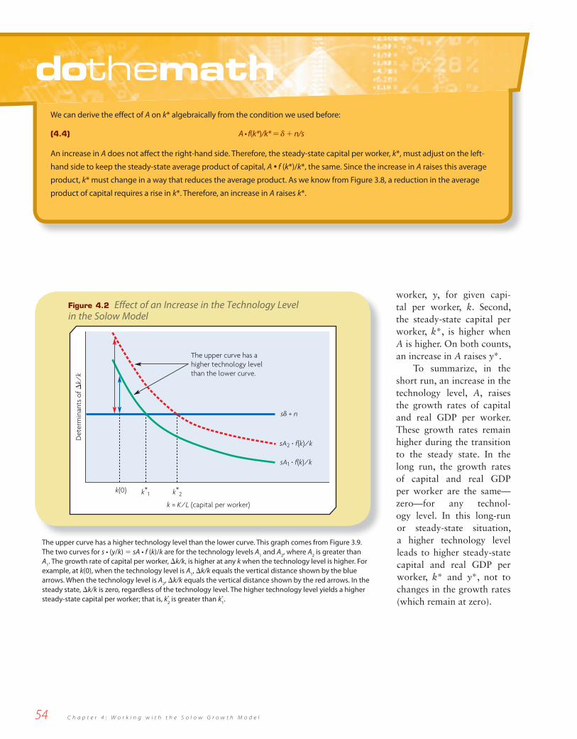
Figure 4.2 compares two levels of technology, A1 and A2, where A2 is greater than A1. Each technology level corresponds to a different curve for s • (y/k) � sA • f(k)/k. The curve with the higher technology level, A2, lies above the other one. Notice that the positions of the two curves are similar to those in Figure 4.1, which considered two values of the saving rate, s. Hence, our analysis of effects from a change in A is similar to that for a change in s.
At the initial capital per worker, k(0), in Figure 4.2, the growth rate of capital per worker, �k/k, is higher with the higher technology level, A2, than with the lower one, A1. In both cases, �k/k declines over time. For the lower technology level, �k/k falls to zero when capital per worker, k, attains the steady-state value k 1
* . For the higher technology level, k rises beyond k 1
* to reach the higher steady-state value k 2
* . Thus, an increase in A re-sults in a higher �k/k over the transition period. In the long run, �k/k still falls to zero, but the steady-state capital per worker, k*, is higher. That is, k 2
* is greater than k 1
* .An increase in the technology level, A, raises the
steady-state real GDP per worker, y* � A • f (k*), for two reasons. First, an increase in A raises real GDP per
W
dothemathWe can determine the steady-state capital per worker, k*, algebraically from the steady-state condition given in equation (3.19).
We repeat this result here:
(4.4) A • f(k*)/k* � � � n/s
An increase in s lowers the right-hand side. Hence, the left-hand side must be lower, and this reduction can occur only through
a decrease in the average product of capital, A • f(k*)/k*. We know from Figure 3.8 that, if A is fi xed, a decrease in the average
product of capital requires an increase in capital per worker, k. Therefore, an increase in s raises k*.
C h a p t e r 4 : W o r k i n g w i t h t h e S o l o w G r o w t h M o d e l54
worker, y, for given capi-tal per worker, k. Second, the steady-state capital per worker, k*, is higher when A is higher. On both counts, an increase in A raises y*.
To summarize, in the short run, an increase in the technology level, A, raises the growth rates of capital and real GDP per worker. These growth rates remain higher during the transition to the steady state. In the long run, the growth rates of capital and real GDP per worker are the same—zero—for any technol-ogy level. In this long-run or steady-state situation, a higher technology level leads to higher steady-state capital and real GDP per worker, k* and y*, not to changes in the growth rates (which remain at zero).
Figure 4.2 Effect of an Increase in the Technology Level in the Solow Model
k(0) k*1 k*
2
Det
erm
inan
ts o
f �k/
k
s� + n
sA2 � f(k)/k
sA1 � f(k)/k
k = K/L (capital per worker)
The upper curve has ahigher technology levelthan the lower curve.
The upper curve has a higher technology level than the lower curve. This graph comes from Figure 3.9. The two curves for s • (y/k) � sA • f (k)/k are for the technology levels A
1 and A
2, where A
2 is greater than
A1. The growth rate of capital per worker, �k/k, is higher at any k when the technology level is higher. For
example, at k(0), when the technology level is A1, �k/k equals the vertical distance shown by the blue
arrows. When the technology level is A2, �k/k equals the vertical distance shown by the red arrows. In the
steady state, �k/k is zero, regardless of the technology level. The higher technology level yields a higher steady-state capital per worker; that is, k
2 * is greater than k
1 * .
dothemathWe can derive the eff ect of A on k* algebraically from the condition we used before:
(4.4) A • f(k*)/k* � � � n/s
An increase in A does not aff ect the right-hand side. Therefore, the steady-state capital per worker, k*, must adjust on the left-
hand side to keep the steady-state average product of capital, A • f (k*)/k*, the same. Since the increase in A raises this average
product, k* must change in a way that reduces the average product. As we know from Figure 3.8, a reduction in the average
product of capital requires a rise in k*. Therefore, an increase in A raises k*.
C h a p t e r 4 : W o r k i n g w i t h t h e S o l o w G r o w t h M o d e l56
Changes in Labor Input and the Population Growth Rate
e can consider two types of changes in labor input, L. First, L could change at a point in time because of a sudden shift in
the size of the labor force. Second, a change in the population growth rate could affect the long-term time path of labor input. We begin with a one-time change in L.
A Change in Labor InputChanges in labor input, L, can result from shifts in the labor force. For example, the labor force could decline precipitously due to an epidemic of disease. An extreme case from the mid-1300s is the bubonic plague, or Black Death, which is estimated to have killed about 20% of the European population. The potential loss of life due to the ongoing AIDS epidemic in Africa may be analogous, and there is also a lot of concern about avian fl u. In these examples, physi-cal capital does not change initially, and the starting
capital per worker, k(0) � K(0)/L(0), rises because of the drop in L(0).
Wartime casualties are another source of decrease in the labor force. However, since wartime tends also to destroy physical capital, the effect on capital per worker depends on the circumstances. Migra-tion can also change the labor force. One example is the Mariel boatlift of over 100,000 Cuban refugees, mostly to Miami, in 1980. Another case is the large in-migration to Portugal in the mid-1970s by its citi-zens who had been residing in African colonies. When these colonies became independent, many residents returned to Portugal, and this infl ow raised the do-mestic Portuguese population by about 10%. Finally, in Israel in the 1990s, the roughly 1,000,000 Russian Jewish immigrants constituted about 20% of Israel’s 1990 population.
Figure 3.8 showed the path of labor input, L, start-ing at L(0) and then growing at the constant rate n. In Figure 4.3, we assume that the initial level of labor input rises from L(0) to L(0) while n does not change. Thus, we are considering a proportionate increase in the level of labor input, L, in each year. Since the ini-tial stock of capital, K(0), does not change, the increase in L(0) decreases the initial capital per worker, k(0) �K(0)/L(0).
Figure 4.4 considers the effects of an increase in the level of labor input. The rise in initial labor from L(0) to L(0) reduces the initial capital per worker from k(0)
to k(0). However, a key point is that the curve for s • (y/k) and the horizontal line at s� � n do not change. The reduction in k(0) raises the initial aver-age product of capital, y/k (see Figure 3.9) and leads, thereby, to a higher s • (y/k) along the unchanged curve. Consequently, the growth rate of capital per worker, �k/k, rises initially. We can see this result in Figure 4.3 because the vertical distance between the s • (y/k) curve and the s� � nline is greater at k(0)
Figure 4.3 An Increase in the Level of Labor Input
Laborinput (L)
L(0)
0
L(0)
Time
In year 0, labor input jumps upward from L (0) to L (0). The population growth rate, n, does not change.
C h a p t e r 4 : W o r k i n g w i t h t h e S o l o w G r o w t h M o d e l 57
(the red arrows) than at k(0) (the blue arrows). The growth rate �k/k remains higher dur-ing the transition to the steady state. However, �k/k still declines toward its long-run value of zero. Moreover, the steady-state capital per work-er, k*, is the same whether labor input starts at L(0) or L(0). Thus, if L(0) is twice as large as L(0), the long-run level of capital, K, is also twice as large (so that capital per worker remains the same). Since k* is unchanged, we also have that real GDP per worker, y*, does not change. In the long run, an economy with twice as much labor has twice as much real GDP, Y.
To summarize, in the short run, an increase in labor input, L(0), raises the growth rates of capital and real GDP per worker. These growth rates remain higher during the transition to the steady state. In the long run, the growth rates of capital and real GDP per worker are the same— zero—for any level of labor input, L(0). Moreover, the steady-state capital and real GDP per worker, k* and y*, are the same for any L. Thus, in the long run, an economy with twice as much labor input has twice as much capital and real GDP.
Figure 4.4 Effect of an Increase in Labor Input in the Solow Model
k(0)
L(0) L(0)
k(0) k*
Det
erm
inan
ts o
f �k/
k
s� + n
s � (y/k)
k = K/L (capital per worker)
The increase in L(0) lowers k(0) and therefore raises �k/k.
This graph comes from Figure 3.10. If the initial level of labor input rises from L (0) to L (0), the initial capi-tal per worker declines from k (0) � K (0)/L (0) to k(0) � K (0)/L (0). Therefore, the growth rate of capital per worker, �k/k, rises initially. Note that the vertical distance shown by the red arrows is larger than that shown by the blue arrows. The steady-state capital per worker, k*, is the same for the two values of L (0).
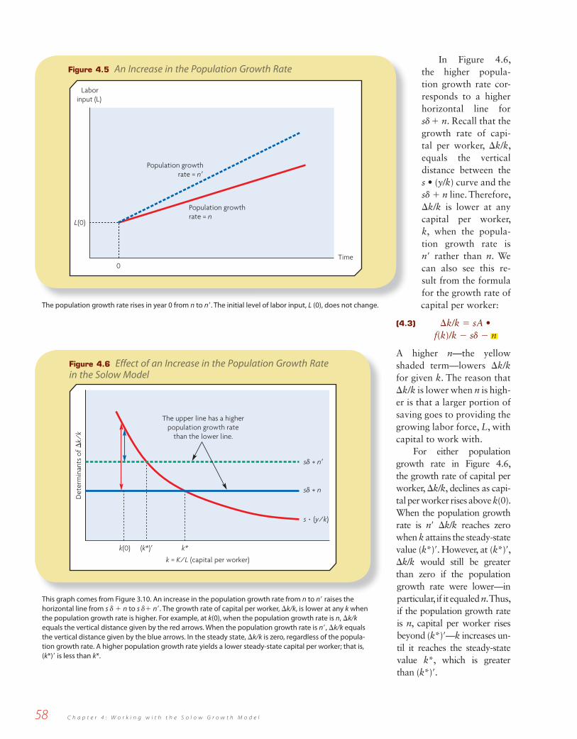
A Change in the Population Growth RateFigure 4.5 shows an increase in the population growth rate from n to n. We assume now that the initial pop-ulation and, hence, level of labor input, L(0), do not change. Thus, the initial capital per worker, k(0), does not change.
dothemathWe can again work out the steady-state results algebraically from the condition
(4.4) A • f(k*)/k* � � � n/s
Note that A, s, n, and � are constant, and the level of labor input, L, does not enter into the equation. Therefore, the steady-state
capital per worker, k*, does not change when L changes.
C h a p t e r 4 : W o r k i n g w i t h t h e S o l o w G r o w t h M o d e l58
In Figure 4.6, the higher popula-tion growth rate cor-responds to a higher horizontal line for s� � n. Recall that the growth rate of capi-tal per worker, �k/k, equals the vertical distance between the s • (y/k) curve and the s� � n line. Therefore, �k/k is lower at any capital per worker, k, when the popula-tion growth rate is n rather than n. We can also see this re-sult from the formula for the growth rate of capital per worker:
(4.3) �k/k � sA • f(k)/k � s� � n
A higher n—the yellow shaded term—lowers �k/kfor given k. The reason that �k/k is lower when n is high-er is that a larger portion of saving goes to providing the growing labor force, L, with capital to work with.
For either population growth rate in Figure 4.6, the growth rate of capital per worker, �k/k, declines as capi-tal per worker rises above k(0). When the population growth rate is n �k/k reaches zero when k attains the steady-state value (k*). However, at (k*), �k/k would still be greater than zero if the population growth rate were lower—in particular, if it equaled n. Thus, if the population growth rate is n, capital per worker rises beyond (k*)—k increases un-til it reaches the steady-state value k*, which is greater than (k*).
Figure 4.5 An Increase in the Population Growth Rate
Laborinput (L)
L(0)
0Time
Population growthrate = n
Population growthrate = n
The population growth rate rises in year 0 from n to n. The initial level of labor input, L (0), does not change.
Det
erm
inan
ts o
f �k/
k
k*
k = K/L (capital per worker)
The upper line has a higherpopulation growth rate
than the lower line.
s� + n�
s� + n
s � (y/k)
k(0) (k*)�
This graph comes from Figure 3.10. An increase in the population growth rate from n to n raises the horizontal line from s � � n to s �� n. The growth rate of capital per worker, �k/k, is lower at any k when the population growth rate is higher. For example, at k(0), when the population growth rate is n, �k/k equals the vertical distance given by the red arrows. When the population growth rate is n, �k/k equals the vertical distance given by the blue arrows. In the steady state, �k/k is zero, regardless of the popula-tion growth rate. A higher population growth rate yields a lower steady-state capital per worker; that is, (k*) is less than k*.
Figure 4.6 Effect of an Increase in the Population Growth Rate in the Solow Model
C h a p t e r 4 : W o r k i n g w i t h t h e S o l o w G r o w t h M o d e l 59
Figure 4.6 shows that, at the initial capital per worker, k(0), an increase in the population growth rate from n to n lowers the growth rate of capital per worker, �k/k. The growth rate of real GDP per worker, �y/y, falls correspondingly. Thus, in the short run, a higher n lowers �k/k and �y/y. These growth rates remain lower during the transition to the steady state. However, in the steady state, �k/k and �y/y are zero for any n. That is, a higher n leads to lower steady-state capital and real GDP per worker, k* and y*, not to changes in the growth rates, �k/k and �y/y (which remain at zero). A change in n does affect the steady-state growth rates of the levels of capital and real GDP, �K/K and �Y/Y. An increase in n by 1% per year raises the steady-state values of �K/K and �Y/Y by 1% per year.
We can see from Figure 4.6 that an increase in the depreciation rate, �, affects the steady-state capi-tal per worker in the same way as an increase in the population growth rate, n. This result follows because equation (4.3) involves the term s� � n, which can rise either from an increase in n or an increase in �. The kind of analysis that we carried out for an increase in n tells us that an increase in � lowers the growth rates of capital and real GDP per worker, �k/k and �y/y, in the short run. In the steady state, an increase in �leads to lower capital and real GDP per worker, k* and y*, not to changes in �k/k and �y/y, which remain at zero.2
2 One diff erence is that an increase in n raises the steady-state growth rates of the levels of capital and real GDP, (�K /K)* and (�Y /Y )*, whereas an increase in ffl does not aff ect these steady-state growth rates.
Convergencene of the most important questions about economic growth is whether poor coun-tries tend to converge or catch up to rich countries. Is there a systematic tendency for low-
income countries like those in Africa to catch up to the rich OECD countries? We will start our answer to this question by seeing what the Solow model says about convergence. Then we will look at how the facts on convergence match up with the Solow model.
Convergence in the Solow ModelTo study convergence, we focus on the transition for cap-ital per worker, k, as it rises from its initial value, k(0), to its steady-state value, k*. In Figure 3.11, we see that k* works like a target or magnet for k during the transition. Therefore, an important part of our analysis of conver-gence concerns the determination of k*. We have stud-ied how k* depends on the saving rate, s, the technology level, A, the population growth rate, n, the depreciation rate, �, and the initial level of labor input, L(0). We can summarize these results in the form of a function for k*:
(4.7) k* � k*[s, A, n, �, L(0)]
(�)(�)(�)(�)(0)
dothemathAs usual, we can fi nd the eff ect of n on k* algebraically from the condition
(4.4) A • f(k*)/k* � � � n/s
An increase in n raises the right-hand side of the equation. Hence, the steady-state average product of capital, A • f (k *)/k* �
y */k*, has to rise on the left-hand side. Because of diminishing average product of capital (Figure 3.9), this change requires a
decrease in k*. Therefore, as we already found, an increase in n reduces k*.
C h a p t e r 4 : W o r k i n g w i t h t h e S o l o w G r o w t h M o d e l60
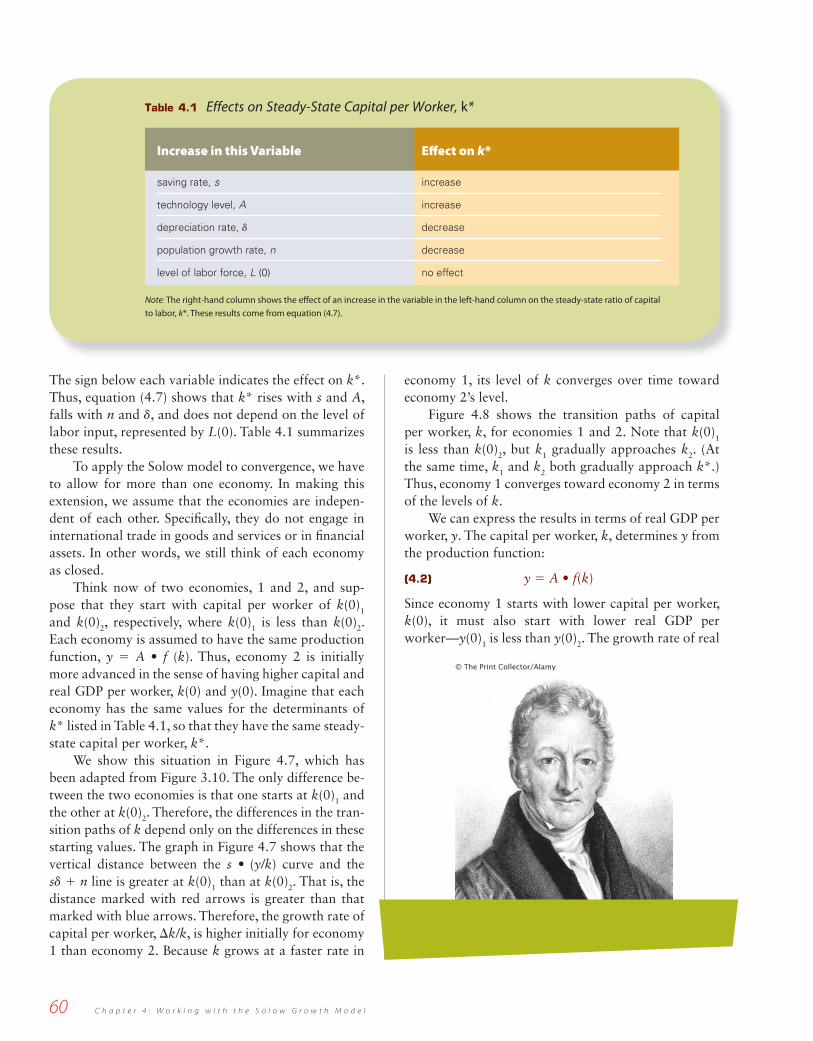
The sign below each variable indicates the effect on k*. Thus, equation (4.7) shows that k* rises with s and A, falls with n and �, and does not depend on the level of labor input, represented by L(0). Table 4.1 summarizes these results.
To apply the Solow model to convergence, we have to allow for more than one economy. In making this extension, we assume that the economies are indepen-dent of each other. Specifi cally, they do not engage in international trade in goods and services or in fi nancial assets. In other words, we still think of each economy as closed.
Think now of two economies, 1 and 2, and sup-pose that they start with capital per worker of k(0)1
and k(0)2, respectively, where k(0)1 is less than k(0)2. Each economy is assumed to have the same production function, y � A • f (k). Thus, economy 2 is initially more advanced in the sense of having higher capital and real GDP per worker, k(0) and y(0). Imagine that each economy has the same values for the determinants of k* listed in Table 4.1, so that they have the same steady-state capital per worker, k*.
We show this situation in Figure 4.7, which has been adapted from Figure 3.10. The only difference be-tween the two economies is that one starts at k(0)1 and the other at k(0)2. Therefore, the differences in the tran-sition paths of k depend only on the differences in these starting values. The graph in Figure 4.7 shows that the vertical distance between the s • (y/k) curve and the s� � n line is greater at k(0)1 than at k(0)2. That is, the distance marked with red arrows is greater than that marked with blue arrows. Therefore, the growth rate of capital per worker, �k/k, is higher initially for economy 1 than economy 2. Because k grows at a faster rate in
economy 1, its level of k converges over time toward economy 2’s level.
Figure 4.8 shows the transition paths of capital per worker, k, for economies 1 and 2. Note that k(0)1
is less than k(0)2, but k1 gradually approaches k2. (At the same time, k1 and k2 both gradually approach k*.) Thus, economy 1 converges toward economy 2 in terms of the levels of k.
We can express the results in terms of real GDP per worker, y. The capital per worker, k, determines y from the production function:
(4.2) y � A • f(k)
Since economy 1 starts with lower capital per worker, k(0), it must also start with lower real GDP per worker—y(0)1 is less than y(0)2. The growth rate of real
Table 4.1 Effects on Steady-State Capital per Worker, k*
Increase in this Variable Eff ect on k*
saving rate, s increase
technology level, A increase
depreciation rate, � decrease
population growth rate, n decrease
level of labor force, L (0) no effect
Note: The right-hand column shows the eff ect of an increase in the variable in the left-hand column on the steady-state ratio of capital
to labor, k*. These results come from equation (4.7).
C h a p t e r 4 : W o r k i n g w i t h t h e S o l o w G r o w t h M o d e l 61
GDP per worker re-lates to the growth rate of capital per worker from equation (3.8), which we repeat:
(4.8) �y/y � � • (�k/k)
where � is the capital-share coeffi cient. (We assume that � is the same in the two econo-mies.) We showed in Figure 4.7 that �k/k was higher initially in economy 1 than in economy 2. Therefore, �y/y is also higher ini-tially in economy 1. Hence, economy 1’s real GDP per worker, y, converges over time to-ward economy 2’s real GDP per worker. The transition paths for y in the two economies look like those shown for k in Figure 4.8.
To summarize, the Solow model says that a poor economy—with low capital and real GDP per worker—grows faster than a rich one. The reason is the di-minishing average prod-uct of capital, y/k. A poor economy, such as econo-my 1 in Figure 4.7, has the advantage of having a high average product of capital, y/k. This high average product explains why the growth rates of capital and real GDP per worker are higher than in the initially more advanced economy, eco-nomy 2. Thus, the So-low model predicts that poorer economies tend to
Figure 4.8 Convergence and Transition Paths for Two Economies
k (capitalper worker)
Time0
k(0)1
k(0)2
k*
k1 converges over time toward k2, whilek1 and k2 both converge toward k*.
k1
k2
Economy 1 starts at capital per worker k(0)1 and economy 2 starts at k(0)2, where k(0)1 is less than k(0)2. The two economies have the same steady-state capital per worker, k*, shown by the dashed blue line. In each economy, k rises over time toward k*. However, k grows faster in economy 1 because k(0)1 is less than k(0)2. (See Figure 4.7.) Therefore, k1 converges over time toward k2.
Det
erm
inan
ts o
f �k/
k
k = K/L (capital per worker)
s� + n
s � (y/k)
k(0)1 k(0)2 k*
Economy 1 growsfaster than economy 2.
This graph comes from Figure 3.10. Economy 1 starts with lower capital per worker than economy 2—k(0)1 is less than k(0)2. Economy 1 grows faster initially because the vertical distance between the s • (y/k) curve and the s� � n line is greater at k(0)1 than at k(0)2. That is, the distance marked by the red arrows is greater than that marked by the blue arrows. Therefore, capital per worker in economy 1, k1, converges over time toward that in economy 2, k2.
C h a p t e r 4 : W o r k i n g w i t h t h e S o l o w G r o w t h M o d e l62
group of countries. We already looked, in Figure 3.3, at growth rates of real GDP per person from 1960 to 2000. To apply the Solow model to these data, we have to translate from amounts per worker to amounts per person. The formula for real GDP per person is again
real GDP per person � (real GDP per worker) • (workers/population)
steady-state capital and real GDP per worker. According to
Malthus, this process would continue until the steady-state
real income per person fell to the subsistence level.
Malthus’s view on the relation between real income
per person and life expectancy is reasonable. Data across
countries show that higher real GDP per person matches up
closely with higher life expectancy at birth.3 However, Mal-
thus’s idea about fertility seems unreasonable. At least in the
cross-country data since 1960, higher real GDP per person
matches up with lower fertility.4 In fact, this relation is so
strong that higher real GDP per person matches up with a
lower population growth rate, even though countries with
higher real GDP per person have higher life expectancy.
We can modify the Solow model to include Malthus’s
idea that population growth is endogenous. However,
contrary to Malthus, we should assume a negative eff ect
of real GDP per person—and, hence, of capital per worker,
k—on the population growth rate, n.
The condition for the growth rate of capital per
worker is again
(4.3) �k/k � sA • f(k/k) � s� � n
During the transition to the steady state, a rise in k
reduced the average product of capital, y/k, and thereby
decreased the growth rate of capital per worker, �k/k.
Now we have that a rise in k also lowers n. This change
raises �k/k and, thus, off sets the eff ect from a reduced
average product of capital. Hence, a declining population
growth rate is one reason why rich societies can sustain
growing capital and real GDP per worker for a long time.
Endogenous Population GrowthOur analysis treated the population growth rate, n, as
exogenous—determined outside of the model. However,
since the writings of Thomas Malthus (1798), economists
have argued that population growth responds to economic
variables. Malthus was a British economist and minister
who wrote his Essay on Population in 1798. He argued that
an increase in real income per person raised population
growth by improving life expectancy, mainly through better
nutrition but also through improved sanitation and medical
care. Another infl uence, Malthus believed, was that higher
income encouraged greater fertility. He thought that birth
rates would rise as long as real income per person exceeded
a subsistence level, which is the amount needed to pay for
the basic necessities of life.
We can incorporate Malthus’s ideas about population
growth into the Solow model. In Figure 3.10, for a given pop-
ulation growth rate, n, the economy approaches a steady-
state capital per worker, k*, and a corresponding real NDP
per worker, y* � A • f (k *) � �k *, which equals real national
income per worker. The real income per person is then
real income per person � (real NDP per worker) � (workers/population)
The last term on the right-hand side is the labor-force par-
ticipation rate, which we assume to be fi xed.
When household real income per person rose above
the subsistence level, Malthus believed that the population
growth rate would rise. Figure 4.6 showed the eff ect from a
rise in the population growth rate; this change lowered the
EXTENDING THE MODEL
converge over time toward richer ones in terms of the levels of capital and real GDP per worker.
Facts About Convergence The main problem with these predictions about conver-gence is that they confl ict with the evidence for a broad
3 Although this relation is suggestive, it does not prove that the causation is from higher real income per person to greater life expectancy, rather than the reverse. In fact, both directions of causation seem to be important. 4 This relation does not prove that the causation is from higher real income per person to lower fertility, rather than the reverse. In fact, the reverse eff ect is predicted by the Solow model. If a society chooses, perhaps for cultural reasons, to have higher fertility and population growth, the model predicts lower steady-state real GDP per worker. In practice, both directions of causation seem to be important.
C h a p t e r 4 : W o r k i n g w i t h t h e S o l o w G r o w t h M o d e l 63
The ratio of work-ers to population is the labor-force par-ticipation rate, which we have assumed to be constant. For ex-ample, if the ratio is around one-half, as in recent U.S. experience, real GDP per person is about one-half of real GDP per worker.
With this transla-tion, we fi nd that the Solow model predicts convergence for real GDP per person. Spe-cifi cally, the model predicts that a lower level of real GDP per person would match up with a high-er subsequent growth rate of real GDP per person.
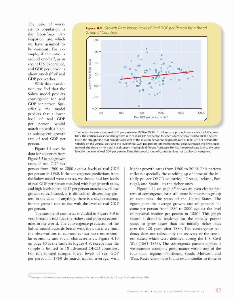
Figure 4.9 uses the data for countries from Figure 3.3 to plot growth rates of real GDP per person from 1960 to 2000 against levels of real GDP per person in 1960. If the convergence predictions from the Solow model were correct, we should fi nd low levels of real GDP per person matched with high growth rates, and high levels of real GDP per person matched with low growth rates. Instead, it is diffi cult to discern any pat-tern in the data—if anything, there is a slight tendency for the growth rate to rise with the level of real GDP per person.
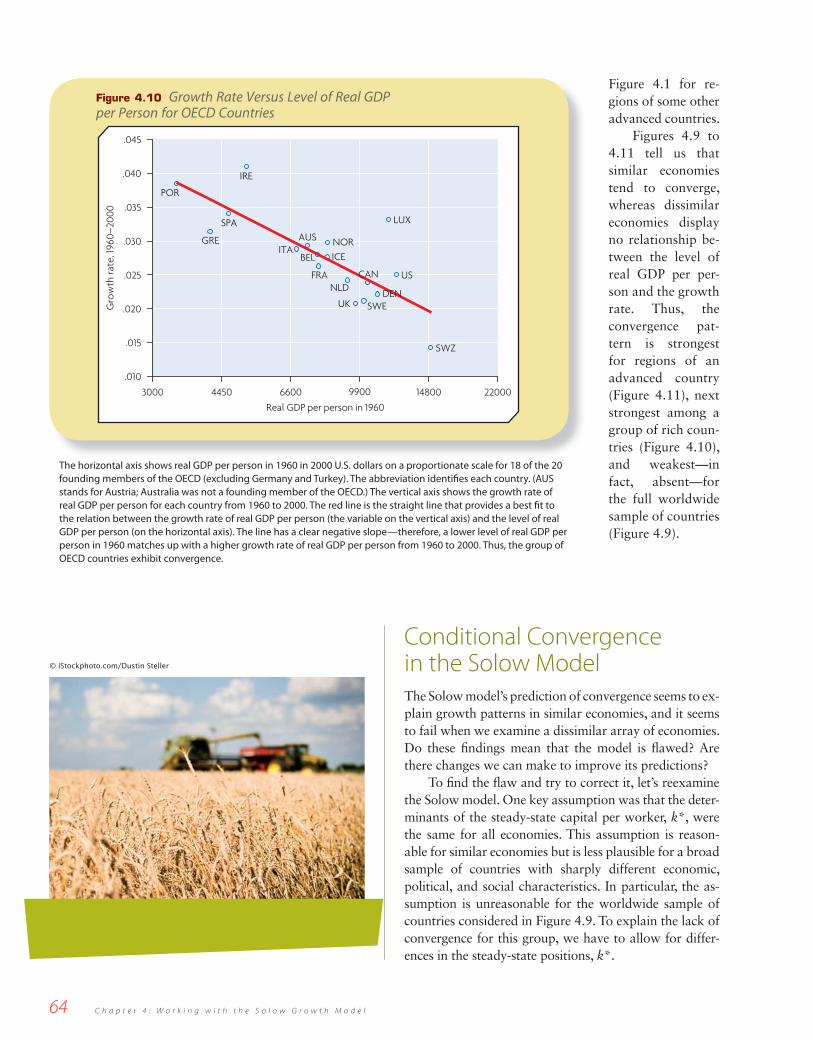
The sample of countries included in Figure 4.9 is very broad; it includes the richest and poorest econo-mies in the world. The convergence prediction of the Solow model accords better with the data if we limit the observations to economies that have more simi-lar economic and social characteristics. Figure 4.10 on page 65 is the same as Figure 4.9, except that the sample is limited to 18 advanced OECD countries. For this limited sample, lower levels of real GDP per person in 1960 do match up, on average, with
Figure 4.9 Growth Rate Versus Level of Real GDP per Person for a Broad Group of Countries
–.04
–.02
.00
.02
.04
.06
.08
150 400 1100 3000 8100 22000Real GDP per person in 1960
Gro
wth
rate
, 196
0–20
00
The horizontal axis shows real GDP per person in 1960 in 2000 U.S. dollars on a proportionate scale for 112 coun-tries. The vertical axis shows the growth rate of real GDP per person for each country from 1960 to 2000. The red line is the straight line that provides a best fi t to the relation between the growth rate of real GDP per person (the variable on the vertical axis) and the level of real GDP per person (on the horizontal axis). Although this line slopes upward, the slope is—in a statistical sense—negligibly diff erent from zero. Hence, the growth rate is virtually unre-lated to the level of real GDP per person. Thus, this broad group of countries does not display convergence.
5 We use personal income because data on gross state product are unavailable for the U.S. states for the period since 1880.
higher growth rates from 1960 to 2000. This pattern reflects especially the catching up of some of the ini-tially poorer OECD countries—Greece, Ireland, Por-tugal, and Spain—to the richer ones.
Figure 4.11 on page 65 shows an even clearer pat-tern of convergence for a still more homogenous group of economies—the states of the United States. The fi gure plots the average growth rate of personal in-come per person from 1880 to 2000 against the level of personal income per person in 1880.5 This graph shows a dramatic tendency for the initially poorer states to grow faster than the initially richer ones over the 120 years after 1880. This convergence ten-dency does not refl ect only the recovery of the south-ern states, which were defeated during the U.S. Civil War (1861–1865). The convergence pattern applies if we examine economic performance within any of the four main regions—Northeast, South, Midwest, and West. Researchers have found results similar to those in
C h a p t e r 4 : W o r k i n g w i t h t h e S o l o w G r o w t h M o d e l64
Figure 4.1 for re-gions of some other advanced countries.
Figures 4.9 to 4.11 tell us that similar economies tend to converge, whereas dissimilar economies display no relationship be-tween the level of real GDP per per-son and the growth rate. Thus, the convergence pat-tern is strongest for regions of an advanced country (Figure 4.11), next strongest among a group of rich coun-tries (Figure 4.10), and weakest—in fact, absent—for the full worldwide sample of countries (Figure 4.9).
Figure 4.10 Growth Rate Versus Level of Real GDP per Person for OECD Countries
.010
.015
.020
.025
.030
.035
.040
.045
3000 4450 6600 9900 14800 22000
Real GDP per person in 1960
Gro
wth
rate
, 196
0–20
00
POR
GRE
SPA
IRE
ITAAUS
BEL
FRA
NORICE
NLD
UK SWE
CAN
DEN
LUX
US
SWZ
The horizontal axis shows real GDP per person in 1960 in 2000 U.S. dollars on a proportionate scale for 18 of the 20 founding members of the OECD (excluding Germany and Turkey). The abbreviation identifi es each country. (AUS stands for Austria; Australia was not a founding member of the OECD.) The vertical axis shows the growth rate of real GDP per person for each country from 1960 to 2000. The red line is the straight line that provides a best fi t to the relation between the growth rate of real GDP per person (the variable on the vertical axis) and the level of real GDP per person (on the horizontal axis). The line has a clear negative slope—therefore, a lower level of real GDP per person in 1960 matches up with a higher growth rate of real GDP per person from 1960 to 2000. Thus, the group of OECD countries exhibit convergence.
Conditional Convergence in the Solow ModelThe Solow model’s prediction of convergence seems to ex-plain growth patterns in similar economies, and it seems to fail when we examine a dissimilar array of economies. Do these fi ndings mean that the model is fl awed? Are there changes we can make to improve its predictions?
To fi nd the fl aw and try to correct it, let’s reexamine the Solow model. One key assumption was that the deter-minants of the steady-state capital per worker, k*, were the same for all economies. This assumption is reason-able for similar economies but is less plausible for a broad sample of countries with sharply different economic, political, and social characteristics. In particular, the as-sumption is unreasonable for the worldwide sample of countries considered in Figure 4.9. To explain the lack of convergence for this group, we have to allow for differ-ences in the steady-state positions, k*.
C h a p t e r 4 : W o r k i n g w i t h t h e S o l o w G r o w t h M o d e l 65
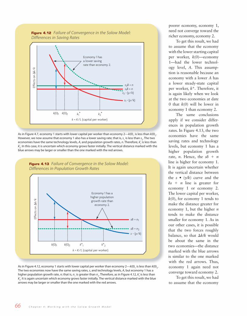
Suppose that coun-tries differ with respect to some of the determi-nants of k* in equation (4.7) and Table 4.1. For example, k* could vary because of differences in saving rates, s, levels of technology, A, and popu-lation growth rates, n.6 Figure 4.12 on page 66 modifi es Figure 4.7 to show how differences in saving rates affect convergence. Economy 1 has the saving rate s1, and economy 2 has the higher saving rate s2. We assume, as in Figure 4.7, that economy 1 has lower initial capital per worker; that is, k(0)1 is less than k(0)2. Remember that the growth rate of capital per worker, �k/k, equals the vertical distance between the s • (y/k) curve and the s� � n line. We see from Figure 4.12 that it is un-certain whether the distance between the s • (y/k) curve and the s� � n line is greater initially for economy 1 or econ-omy 2. The lower capital per worker, k(0), tends to make the distance greater for economy 1, but the lower saving rate, s, tends to make the distance smaller for economy 1. In the graph, these two forces roughly balance, so that �k/k is about the same for the two economies. That is, the distance marked with the blue arrows is similar to the one marked with the red arrows. Therefore, the poorer economy, econo-my 1, does not necessarily converge toward the richer econ-omy, economy 2.
To get the result in Figure 4.12, we had to assume that the economy with lower k(0)—economy 1—had a lower saving rate, s. This assumption is reasonable because an economy with a lower s has a lower steady-state capital per worker, k*. In the long run, an economy’s capital per worker, k, would be close to its steady-state value, k*. Therefore, it is likely when we examine countries at an
arbitrary date, such as date 0, that k(0) will be lower in the economy with the lower s—k(0) tends to be lower in economy 1 than in economy 2. Thus, the pattern that we assumed—a low saving rate matched with a low k(0)—is likely to apply in practice.
We get a similar result if we consider other reasons for differences in the steady-state capital per worker, k*. Sup-pose that the two economies have the same saving rates but that economy 1 has a lower technology level, A, than economy 2. In this case, the two curves for s • (y/k) again look as shown in Figure 4.12.7 Therefore, it is again un-certain whether the vertical distance between the s • (y/k) curve and the s� � n line is greater for economy 1 or econ-omy 2. The lower capital per worker, k(0), tends to make the distance greater for economy 1, but the lower A tends to make the distance smaller for economy 1. As before, it is possible that the two forces roughly balance, so that �k/k is about the same for the two economies. Thus, the
Figure 4.11 Growth Rate Versus Level of Income per Person for U.S. States, 1880–2000
500 1000
Gro
wth
rate
of p
erso
nal i
ncom
e pe
r per
son,
1880
–20
00
2500 5000
.005
.010
.015
.020
.025 NC
SC FL
AR
TNAL
MS
VAGA
WVTX
NMKY
KS
UTLA
MEIN
NE
WI
MO
IA
VT
MD
MI
MN
OH
NDSD
NH
DEILPAWA
OR
NJCT
RI
NY
ID
MA
WY COCA
AZ
MTNV
The horizontal axis shows real personal income per person in 1982–1984 U.S. dollars on a proportionate scale for 47 U.S. states. The two-letter abbreviation identifi es the state. (Alaska, the District of Columbia, Hawaii, and Oklahoma are excluded.) The vertical axis shows the growth rate of real personal income per person for each state from 1880 to 2000. The solid line is the straight line that provides a best fi t to the relation between the growth rate of income per person (the variable on the vertical axis) and the level of income per person (on the horizontal axis). The line has a clear negative slope—therefore, a lower level of income per person in 1880 matches up with a higher growth rate of income per person from 1880 to 2000. Thus, the U.S. states exhibit convergence.
6 Levels of population and the labor force vary greatly across countries, but the level of labor input, represented by L (0), does not aff ect k* in the model. The depreciation rate, �, probably does not vary systematically across countries.7 In this case, unlike in Figure 4.12, the �s � n lines are the same for the two countries.
C h a p t e r 4 : W o r k i n g w i t h t h e S o l o w G r o w t h M o d e l66
poorer economy, economy 1, need not converge toward the richer economy, economy 2.
To get this result, we had to assume that the economy with the lower starting capital per worker, k(0)—economy 1—had the lower technol-ogy level, A. This assump-tion is reasonable because an economy with a lower A has a lower steady-state capital per worker, k*. Therefore, it is again likely when we look at the two economies at date 0 that k(0) will be lower in economy 1 than economy 2.
The same conclusions apply if we consider differ-ences in population growth rates. In Figure 4.13, the two economies have the same saving rates and technology levels, but economy 1 has a higher population growth rate, n. Hence, the s� � nline is higher for economy 1. It is again uncertain whether the vertical distance between the s • (y/k) curve and the �s � n line is greater for economy 1 or economy 2. The lower capital per worker, k(0), for economy 1 tends to make the distance greater for economy 1, but the higher ntends to make the distance smaller for economy 1. As in our other cases, it is possible that the two forces roughly balance, so that �k/k would be about the same in the two economies—the distance marked with the blue arrows is similar to the one marked with the red arrows. Thus, economy 1 again need not converge toward economy 2.
To get this result, we had to assume that the economy
Figure 4.13 Failure of Convergence in the Solow Model: Differences in Population Growth Rates
k*2k*1
Effe
cts
on �
k/k
Economy 1 has ahigher populationgrowth rate than
economy 2.
s � (y/k)
s� + n1
s� + n2
k = K/L (capital per worker)
k(0)2 k(0)1
As in Figure 4.12, economy 1 starts with lower capital per worker than economy 2—k(0)1 is less than k(0)
2.
The two economies now have the same saving rates, s, and technology levels, A, but economy 1 has a higher population growth rate, n; that is, n
1 is greater than n
2. Therefore, as in Figure 4.12, k
1 * is less than
k 2 * . It is again uncertain which economy grows faster initially. The vertical distance marked with the blue
arrows may be larger or smaller than the one marked with the red arrows.
Figure 4.12 Failure of Convergence in the Solow Model: Differences in Saving Rates
As in Figure 4.7, economy 1 starts with lower capital per worker than economy 2—k(0)1 is less than k(0)
2.
However, we now assume that economy 1 also has a lower saving rate; that is, s1 is less than s
2. The two
economies have the same technology levels, A, and population growth rates, n. Therefore, k 1 * is less than
k 2 * . In this case, it is uncertain which economy grows faster initially. The vertical distance marked with the
blue arrows may be larger or smaller than the one marked with the red arrows.
C h a p t e r 4 : W o r k i n g w i t h t h e S o l o w G r o w t h M o d e l 67
with the lower start-ing capital per worker, k(0)— economy 1—had the higher population growth rate, n. This as-sumption makes sense because an economy with a higher n has a lower steady-state capital per worker, k*. Therefore, it is again likely when we look at the two economies at date 0 that k(0) will be lower in economy 1 than economy 2.
Now let’s gener-alize the conclusions from our three cases. In each case, economy 1 had a characteristic—lower saving rate, s, lower technology level, A, higher population growth rate, n—that led to a lower steady-state capital per worker, k*. For a given starting capi-tal per worker, k(0), each of the three characteristics tended to make country 1’s initial growth rate less than economy 2’s initial growth rate. We see these effects in Figures 4.12 and 4.13. At a given k(0), the vertical dis-tance between the s • (y/k) curve and the s� � n line is smaller if s or A is lower or if n is higher.
Since economy 1 has lower k*, it is also likely to have lower initial capital per worker, k(0). The lower k(0) tends to make economy 1 grow faster than economy 2—the convergence force shown in Figure 4.7. Whether economy 1 grows faster or slower overall than economy 2 depends on the offset of two forces. The lower k(0) generates faster growth in econ-omy 1, but the lower k* generates slower growth in economy 1. It is possible that the two forces roughly balance, so that the two economies grow at about the same rate. That is, we need not fi nd convergence.
Figure 4.14 shows the transition paths of capital per worker, k, for the two economies. We assume that economy 1 starts with a lower capital per worker—k(0)1
is less than k(0)2—and also has a lower steady-state capital per worker— k 1
* is less than k 2 * . The graph shows
that capital per worker in each economy converges
toward its own steady-state level—k1 toward k 1 * , and k2
toward k 2 * . However, since k 1
* is less than k 2 * , k1 does not
converge toward k2.We can summarize our fi ndings for the growth rate
of capital per worker in an equation:
The function � indicates how �k/k depends on the ini-tial capital per worker, k(0), and the steady-state capital per worker, k*. The minus sign under k(0) signifi es that, for given k*, a decrease in k(0) raises �k/k. The plus sign under k* means that, for given k(0), a rise in k* increases �k/k.
Figure 4.14 Failure of Convergence and Transition Paths for Two Economies
k (capitalper worker)
Time0
k(0)1
k(0)2
k2
k1
k*1
k*2
Economy 1 has lower k(0) and lower k*—therefore, k1 does not converge toward k2.
As in Figures 4.12 and 4.13, economy 1 has a lower starting capital per worker—k(0)1 is less than k(0)
2—and also
has a lower steady-state capital per worker— k1* (the dashed brown line) is less than k
2* (the dashed blue line). Each
capital per worker converges over time toward its own steady-state value: k1 (the red curve) toward k
1* , and k
2 (the
green curve) toward k2* . However, since k
1* is less than k
2* , k
1 does not converge toward k
2.
Key equation (conditional convergence in the Solow model):
(4.9) � k/k � �[k(0), k*] (�) (�)
growth rate of capital per worker � function of initial and steady-state capital per worker
C h a p t e r 4 : W o r k i n g w i t h t h e S o l o w G r o w t h M o d e l68
We can interpret the effects in equation (4.9) from the perspective of our equation for the growth rate of capital per worker:
(4.3) �k/k � sA • f(k)/k � s� � n
The negative effect of k(0) in equation (4.9) corresponds in equation (4.3) to a lower initial average product of capital, A • f (k)/k. The positive effect of k* in equation (4.9) corresponds in equation (4.3) to a higher saving rate, s, a higher technology level, A, or a lower popula-tion growth rate, n.
One important result in equation (4.9) is that the negative effect of k(0) on the growth rate, �k/k, holds only in a conditional sense—that is, for a given k*. This pattern is called conditional convergence: A lower k(0) predicts a higher �k/k, conditional on k*. In contrast, the prediction that a lower k(0) raises �k/k without any conditioning is called absolute convergence.
Recall from Figure 4.9 that we do not observe abso-lute convergence for a broad group of countries. We see from equation (4.9) that we can use the Solow model to explain the lack of convergence in this diverse group. Suppose that some countries have low saving rates, low technology levels, or high population growth rates and, therefore, have low steady-state capital per worker, k*. In the long run, capital per worker, k, will be close to k*. Therefore, when we look at date 0 (say, 1960), we tend to fi nd that low values of k(0) match up with low values of k*. A low value of k(0) makes the growth rate of capital per worker, �k/k, high, but a low value of k* makes �k/k low. Thus, the data may show little relation
between k(0) and �k/k. This pattern is consistent with the one found in Figure 4.9 for growth rates and levels of real GDP per person.
Where Do We Stand with the Solow Model?
hen we fi rst consid-ered convergence, we observed that the lack of absolute convergence for a broad group of countries, as in Figure 4.9,
was a failing of the Solow model. Then we found that an extension of the model to consider conditional con-vergence explained this apparent failure. We show in the next chapter that conditional convergence allows us to understand many other features of economic growth in the world.
Although the Solow model has many strengths, we should be clear about what the model does not explain. Most important is the failure to explain how real GDP per person grows in the long run—for example, at a rate of about 2% per year for well over a century in the United States and other advanced countries. In the model, capital per worker—and, hence, real GDP per worker and per person—are constant in the long run. Thus, a key objective of the next chapter is to extend the model to explain long-run economic growth.
W
C h a p t e r 4 : W o r k i n g w i t h t h e S o l o w G r o w t h M o d e l68
A. Review questions1. If the initial level of labor input, L(0), doubles, why
does the steady-state capital stock, K*, double? That is, Figure 4.4 implies that steady-state capital per worker, k*, does not change. How does this result depend on constant returns to scale in the production function?
2. Does population growth, n � 0, lead to growth of output in the long run? Does it lead to growth of output per worker in the long run?
3. What is the meaning of the term convergence? How does absolute convergence differ from conditional convergence?
4. For 112 countries, Figure 4.9 shows that the growth rate of real per capita GDP from 1960 to 2000 bears little relation to the level of real GDP in 1960. Does this fi nding confl ict with the Solow model of eco-nomic growth? How does this question relate to the concept of conditional convergence?
B. Problems for discussion5. Variations in the saving rate Suppose that the saving rate, s, can vary as an
economy develops.
a. The equation for the growth rate of capital per worker, k, is given by
C h a p t e r 4 : W o r k i n g w i t h t h e S o l o w G r o w t h M o d e l 69
(4.1) �k/k � s • (y/k) � s� � n
Is this equation still valid when s is not constant?
b. Suppose that s rises as an economy develops; that is, rich countries save at a higher rate than poor coun-tries. How does this behavior affect the results about convergence?
c. Suppose, instead, that s falls as an economy develops; that is, rich countries save at a lower rate than poor countries. How does this behavior affect the results about convergence?
d. Which case seems more plausible—b or c? Explain.
6. Variations in the population growth rate Suppose that the population growth rate, n,
can vary as an economy develops.
a. The equation for the growth rate of capital per worker, k, is again given from
(4.1) �k/k � s • (y/k) � s� � n
Is this equation still valid when n is not constant?
b. Suppose that n falls as an economy develops; that is, rich countries have lower population growth rates than poor countries. How does this behavior affect the results about convergence?
c. Suppose, instead, that n rises as an economy devel-ops; that is, rich countries have higher population growth rates than poor countries. How does this behavior affect the results about convergence?
d. Which case seems more plausible—b or c? Explain, giving particular attention to the views of Malthus about endogenous population growth.
C h a p t e r 4 : W o r k i n g w i t h t h e S o l o w G r o w t h M o d e l70
chapter appendix
The Rate of Convergence
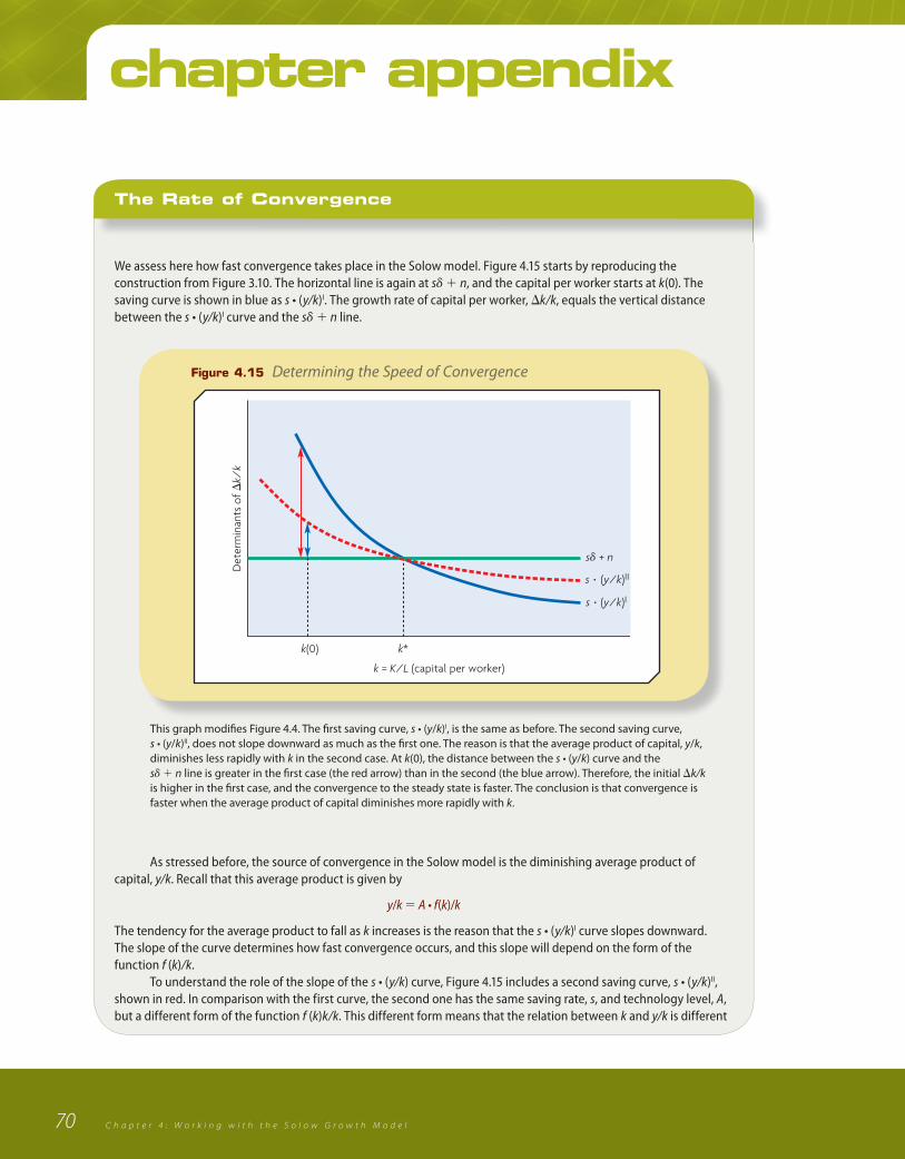
We assess here how fast convergence takes place in the Solow model. Figure 4.15 starts by reproducing the construction from Figure 3.10. The horizontal line is again at s� � n, and the capital per worker starts at k(0). The saving curve is shown in blue as s • (y/k)I. The growth rate of capital per worker, �k/k, equals the vertical distance between the s • (y/k)I curve and the s� � n line.
As stressed before, the source of convergence in the Solow model is the diminishing average product of capital, y/k. Recall that this average product is given by
y/k � A • f(k)/k
The tendency for the average product to fall as k increases is the reason that the s • (y/k)I curve slopes downward. The slope of the curve determines how fast convergence occurs, and this slope will depend on the form of the function f (k)/k. To understand the role of the slope of the s • (y/k) curve, Figure 4.15 includes a second saving curve, s • (y/k)II, shown in red. In comparison with the first curve, the second one has the same saving rate, s, and technology level, A, but a different form of the function f (k)k/k. This different form means that the relation between k and y/k is different
Figure 4.15 Determining the Speed of Convergence
Det
erm
inan
ts o
f �k/
k
k = K/L (capital per worker)
s� + n
s � (y/k)II
s � (y/k)I
k* k(0)
This graph modifi es Figure 4.4. The fi rst saving curve, s • (y/k)I, is the same as before. The second saving curve, s • (y/k)II, does not slope downward as much as the fi rst one. The reason is that the average product of capital, y/k, diminishes less rapidly with k in the second case. At k(0), the distance between the s • (y/k) curve and the s� � n line is greater in the fi rst case (the red arrow) than in the second (the blue arrow). Therefore, the initial �k/k is higher in the fi rst case, and the convergence to the steady state is faster. The conclusion is that convergence is faster when the average product of capital diminishes more rapidly with k.
71C h a p t e r 4 : W o r k i n g w i t h t h e S o l o w G r o w t h M o d e l
for curve II than for curve I. Specifically, at any value of k, the second curve does not slope downward as much as the first one. That is, the average product of capital, y/k, diminishes less rapidly with k in the second case than in the first one. To ease the comparison, we set up the graph so that the two saving curves intersect the s� � n line at the same point. Hence, the steady-state capital per worker, k*, is the same in the two cases. However, at the initial capital per worker, k(0), the vertical distance between the saving curve and the s� � n line is larger in the first case than in the second. In the graph, the first distance is shown by the brown arrows, and the second distance by the green arrows. Therefore, at k(0), �k/k is higher in the first case. The higher growth rate means that k converges more rapidly toward its steady-state level, k*. Hence, we have shown that the rate of convergence is higher when the average product of capital diminishes more rapidly with k. For a given technology level, A, the relation between the average product of capital, y/k, and k depends on the form of the function f (k)/k. To take a concrete example, consider the Cobb-Douglas production function, introduced in the Appendix, Part C to Chapter 3, where f (k) � k�. In this case, the average product of capital is
(4.10) y/k � A • f(k)/k
� Ak�/k
� Ak� • k�1
� Ak(� � 1)
y/k � Ak�(1 � )
Since 0 < � < 1, the average product of capital, y/k, falls as k rises. The value of � determines how fast y/k falls as k rises. If � is close to 1, equation (4.10) says that y/k falls slowly as k rises (curve II in Figure 4.15 is like this). If � is close to zero, y/k falls quickly as k rises (curve I is like this). Generally, the lower � is, the more quickly y/k falls as k rises.To get a quantitative idea about the rate of convergence, consider an intermediate case in which � � 0.5. In this case, the average product of capital is
y/k � Ak�(1/2)
y/k � A/ √ _
k
That is, the average product of capital declines with the square root of k. Recall that the growth rate of k is given by
(4.1) �k/k � s • (y/k) � s� � n
If we substitute y/k � A/√k, we get
(4.11) �k/k � sA/ √ _ k � s� � n
If we specify values for the saving rate, s, the technology level, A, the depreciation rate, �, the rate of population growth, n, and the initial capital per worker, k(0), we can use equation (4.11) to calculate the time path of k. Since we know k(0), equation (4.11) determines k at the next point in time, k(1). Then, given k(1), we can use the equation to calculate k(2). Proceeding in this way, we can calculate k(t) at any time t. Table 4.2 shows the solution for the path of k(t). The calculations assume that the initial capital per worker, k(0), is one-half of its steady-state value, k*. The table reports the values of k/k* and y/y* that prevail after 5 years, 10 years, and so on. Note that it takes about 25 years—roughly a generation—to eliminate half of the initial gap between k and k*. By analogy to radioactive decay in physics, we can define the time for half of the convergence to the steady state to occur as the half-life. Since the ratio k/k* starts at 0.5 and the half-life of the convergence process is 25 years, the ratio reaches 0.75 in 25 years and 0.875 in 50 years. Hence, although capital per worker, k, converges toward k*, the Solow model predicts that this process takes a long time. The same numerical results on half-lives turn out to apply to the adjustment of real GDP per worker, y, to its steady-state level, y*.
72 C h a p t e r 4 : W o r k i n g w i t h t h e S o l o w G r o w t h M o d e l
Table 4.2 The Transition Path in the Solow Model
Year k/k* y/y*
0 0.50 0.71
5 0.56 0.75
10 0.61 0.78
15 0.66 0.81
20 0.71 0.84
25 0.74 0.86
30 0.78 0.88
35 0.81 0.90
40 0.83 0.91
45 0.86 0.93
50 0.88 0.94
Note: The table shows the solution of the Solow model for capital per worker, k, and
real GDP per worker, y. The results are expressed as ratios to the steady-state values,
k/k* and y/y*. The transitional behavior of k and y comes from equation (4.11),
which assumes y � A • √_ k . The calculations assume that k/k* starts at 0.5 and uses
the values n � 0.01 per year and � � 0.05 per year. The values of s, A, and L(0) turn
out not to aff ect the results. The initial value for k/k* also does not matter for the
speed of convergence.
If � is greater than 0.5, the average product of capital, y/k, declines more slowly as k rises, and the convergence to the steady state is less rapid. Therefore, the half-life is more than 25 years. Conversely, if � is less than 0.5, y/k declines more quickly as k rises, and the convergence to the steady state is more rapid. In this case, the half-life is less than 25 years. Many interesting applications have been made for speeds of convergence and half-lives calculated from the Solow model. One implication involves the aftermath of the U.S. Civil War, which ended in 1865. The model says that the southern states from the defeated Confederacy would converge only slowly in terms of real income per person to the richer northern states. (The war reduced the income per person in the south from roughly 80% of the northern level to about 40%.) The quantitative prediction, which turns out to be accurate, is that the convergence process would take more than two generations to be nearly complete. Similarly, with the unification of Germany in 1990, the model predicts that the poor eastern parts from the formerly Communist East Germany would converge, but only slowly, to the richer western regions. (In 1990, the GDP per person of the eastern regions was about one-third of the western level.) This prediction for gradual convergence of real GDP per person accords with the German data for the 1990s.