Workshop on Central Clearingof Derivatives & Risk Management

Marco Avellaneda

Courant Institute NYU

Finance Concepts LLC

Research in Options, IMPA Rio de Janeiro, November 27, 2016

Post-Lehman: Clearing OTC Derivatives

• The financial crisis of 2007-2008 brought attention to systemic risk in world financial markets.

• One of the main concerns was the unregulated market in OTC derivatives

• Credit derivatives were at the center of the collapse of Lehman Brothers,Bear Stearns Co. and the government bailout of AIG and mortgage banks(GSEs).

• Aside from a general overhaul of banking regulations, the derivatives marketsattracted the attention of regulators worldwide.

• The idea that OTC derivatives could be centrally cleared took root in the Fall of 2008 under the auspices of the NY Fed and Timothy Geithner, whowent on to become the U.S. Treasury Secretary under the new ObamaAdministration.

• This led to a focus on the idea of Central Clearing of derivatives, followingthe model practiced by securities markets.

What is a CCP and what is it good for?• Central Clearing is a legal/market framework which is often put in place

to protect the market against systemic risk

• Clearinghouses are in charge of payments, settlement and clearing (registering)trades in a centralized location. This allows, for instance, regulators and investorsto have a better picture of the market and to eliminate credit risk.

• In a bilateral transaction A and B make a trade. If this transaction is notfully paid (e.g. the security is bought on credit) then this creates a credit exposurebetween the counterparties.

• Short-selling equities requires lending/borrowing. All short selling necessarily introduces a credit exposure.

• Repurchase agreements are the standard way to finance fixed-income securities.Repos clearly introduce credit exposure.

Why the interest in CCPs now?

• CCPs have been used in the context of exchange-traded securities and futuresfor many years.

• The 2008 crisis and the bankruptcy of AIG was seen as being exacerbated bythe proliferation of Credit Default Swap transactions. These transactions wereover-the-counter and bilateral. Notional amounts were in the trillions USD.

• If a swap dealer cannot fund his positions, he must unwind them, producinga ``chain reaction’’ in the system (like AIG).

• The idea of creating CCPs for over-the-counter derivatives originated in late 2008and was made more concrete in the Dodd-Frank legislation of 2009.

• International norms were proposed by the Bank of International Settlements in2010-2012 in a series of documents.

• The push for central clearing of derivatives became fully international since 2012.

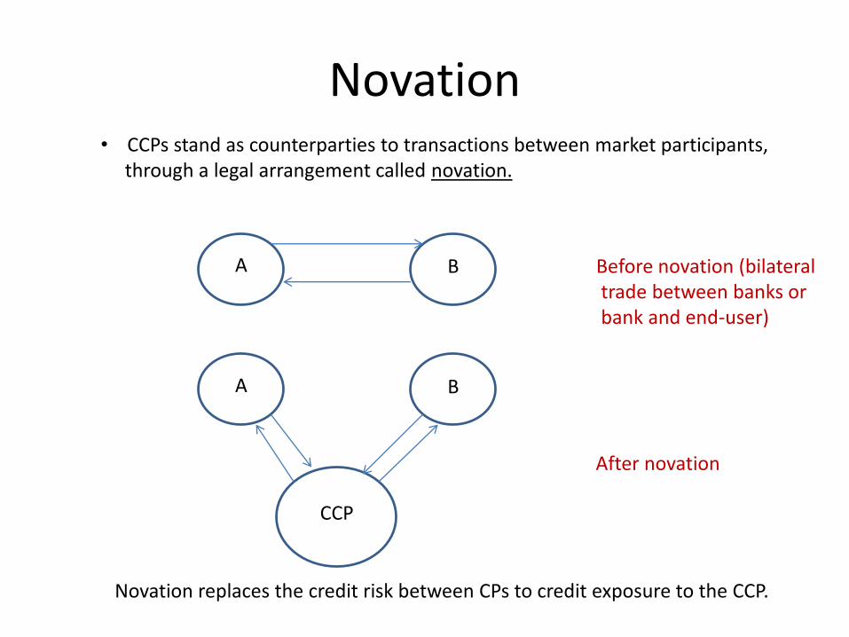
Novation• CCPs stand as counterparties to transactions between market participants,

through a legal arrangement called novation.

A B Before novation (bilateraltrade between banks orbank and end-user)

A B

CCP

After novation

Novation replaces the credit risk between CPs to credit exposure to the CCP.

Netting

A B

C

500 M

300 M250 M

Notional paymentIn case of default(sell protection)

Periodic feepayments (buy protection)

A B

C

CCP

250 M 200 M

50 M

Novation + Netting implies``compression’’

Central Clearing : transparency,Compression, mitigation ofSystemic risk

Central clearing as a financial network

CM1

CM2

CM3

CM4

CM5

CM6CM7

CCP

Clearing members:large banks, BDs

Arrows representcredit exposure

Small circles: non-clearing marketparticipants(e.g., hedge funds,

asset-managers,derivatives end-users,clients of CPs,retail investors)

Central clearing is a specific type of ``financial network’’ as in Hamini, Cont & Minca (2010)

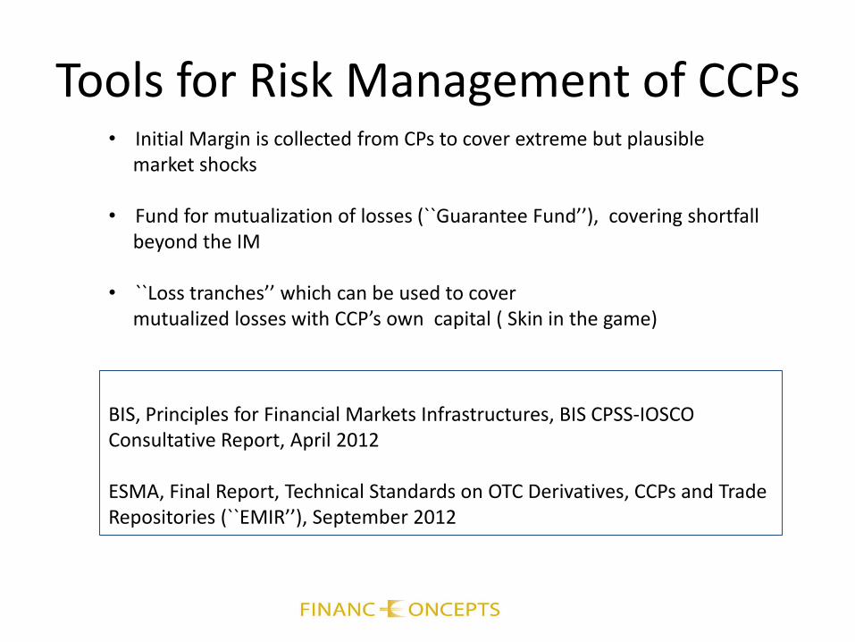
Tools for Risk Management of CCPs • Initial Margin is collected from CPs to cover extreme but plausible

market shocks

• Fund for mutualization of losses (``Guarantee Fund’’), covering shortfallbeyond the IM

• ``Loss tranches’’ which can be used to covermutualized losses with CCP’s own capital ( Skin in the game)

BIS, Principles for Financial Markets Infrastructures, BIS CPSS-IOSCOConsultative Report, April 2012

ESMA, Final Report, Technical Standards on OTC Derivatives, CCPs and TradeRepositories (``EMIR’’), September 2012

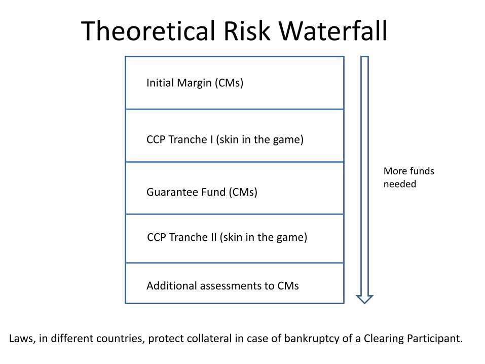
Theoretical Risk Waterfall

Initial Margin (CMs)

CCP Tranche I (skin in the game)

Guarantee Fund (CMs)

CCP Tranche II (skin in the game)

Additional assessments to CMs

More fundsneeded

Laws, in different countries, protect collateral in case of bankruptcy of a Clearing Participant.

Client/House Account

CCP

House Acct

Clients’ Accounts collateral

Collateral +guarantee fund

Typically, each clearing memberholds two accounts: the House accountand the Clients’ account. Both are margined separately.

Client’s securities can be ``in street name’’ (held under CPs name) or in theName of the Ultimate Beneficiary.

Client account segregation is important

Client Clearing (EMIR)

CCPs and clearing members must offer both:– Omnibus client segregation: Separate records / accounts distinguishing between clearing

member's assets and positions and assets and positions of its clients– Individual client segregation: Separate records / accounts distinguishing between assets and

positions of each client of clearing member and any excess margin posted to CCP

CCPs must allow clearing members to open further accounts Requirement to distinguish involves recording in separate accounts, not netting across

accounts and not exposing assets in one account to losses in another

CCPs and clearing members must disclose levels of protection and costs - must be reasonable commercial terms

CCPs must commit to trigger procedure for porting - if clearing member defaults and client requests, transfer client positions and assets to another clearing member that has agreed to step in - omnibus and individual accounts

CCPs can actively manage their risks by liquidating positions and assets if this cannot be done within a pre-defined timeframe

Client collateral can only be used to cover positions held for relevant client account and any surplus on a clearing member default should be returned to client or, if not possible, to clearing member for relevant client account

``Omnibus’’ Segregation

Client 1

Client 2

Client 3

Clients 1, 2 +3 Clients, 1, 2 + 3

Clearing Member (books + records)

CCP (books + records)

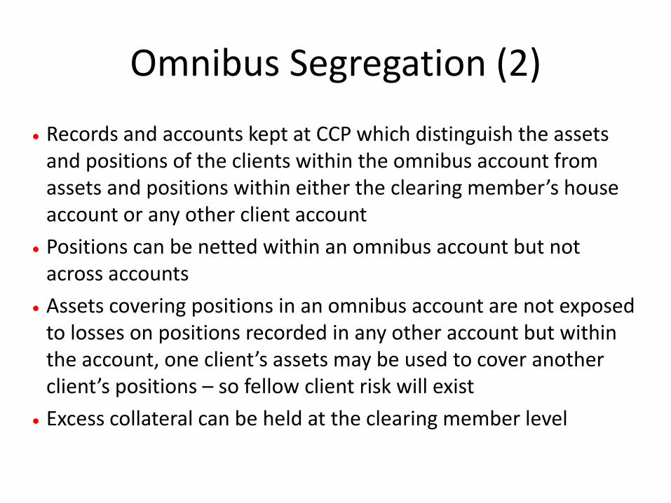
Omnibus Segregation (2)

Records and accounts kept at CCP which distinguish the assets and positions of the clients within the omnibus account from assets and positions within either the clearing member’s house account or any other client account

Positions can be netted within an omnibus account but not across accounts

Assets covering positions in an omnibus account are not exposed to losses on positions recorded in any other account but within the account, one client’s assets may be used to cover another client’s positions – so fellow client risk will exist

Excess collateral can be held at the clearing member level

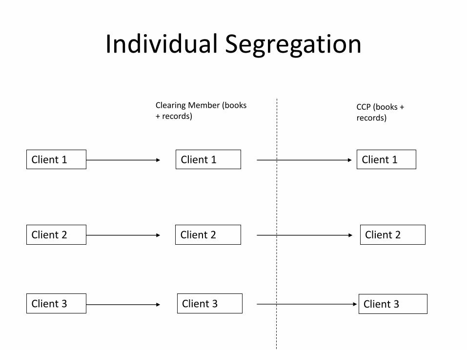
Individual Segregation

Client 1

Client 2

Client 3

Clearing Member (books + records)

CCP (books + records)

Client 1

Client 2

Client 3

Client 1

Client 2

Client 3

Individual Segregation

Positions and assets distinguished from the positions and assets of any other client and the clearing member’s house account

Positions within the account can be netted but positions cannot be netted across accounts

Assets covering positions recorded in the account cannot be used to cover losses connected to positions recorded in any other account, so no fellow client risk

Any collateral called by the clearing member which is in excess of that called by the CCP must be passed to the CCP and not held by the clearing member

Porting a Client Account (if CM defaults)

Clearing Member

CCP

Client

Alternative Clearing Member

Back off contracts, clearing agreement, security interest in favour of the client, collateral

Cleared contract, CCP rules, collateral

OTC Counterparty

OTC derivative trade, non-clearing master agreement

Porting of positions and assets takes place on clearing member default

Should all OTC derivatives be centrally cleared?• This is a complex question, which cannot be answered by a simple ``yes/no’’.

• OTC markets are private markets (confidentiality a plus)

• Notional amounts are very large compared to typical contract sizes/lot sizesin listed markets

• Derivatives can be ``bespoke’’, so the CCP would need to be equipped with complex risk-management systems.

• OTC derivatives can be hedges to other, even more bespoke transactions whichare difficult to clear. Central clearing of one ``leg’’ of a transaction but notanother can introduce large costs to market participants.

• Are CCPs equipped to handle the massive credit exposure of the derivativesmarket?

These questions have been addressed in a Incremental way (asset class by asset class)the answers depend on the legal system of the country and on existing market practices pre-crisis.

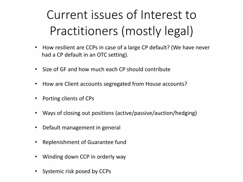
Current issues of Interest to Practitioners (mostly legal)

• How resilient are CCPs in case of a large CP default? (We have neverhad a CP default in an OTC setting).

• Size of GF and how much each CP should contribute

• How are Client accounts segregated from House accounts?

• Porting clients of CPs

• Ways of closing out positions (active/passive/auction/hedging)

• Default management in general

• Replenishment of Guarantee fund

• Winding down CCP in orderly way

• Systemic risk posed by CCPs

Today’s Major Clearing Houses

Inter bank payments: ACH (check clearing)

Securities: DTCC, FICC, LCH.Clearnet, Eurex Clearing (stocks, bonds)

Derivatives: CME Group, LCH.Clearnet, Intercontinental Exchange (ICE), ICE Clear Europe (swaps, credit default swaps)

Exchange-traded equity Options: The Options Clearing Corporation

BM&F Bovespa: manages 4 CCPs for different asset classes (likeCME Group, which clears commodities, financials, and some OTC)

Hong Kong Exchanges and Clearing Ltd.: Securities and derivatives clearingBoth exchange-traded and OTC

DTCC

• DTC: clears securities: Equities and Corporate Bonds

• DTCC DerivSERV: Trade repository for OTC Credit Derivatives

• DTCC LoanSERV: Repository for Loans

• FICC: Fixed-income clearing corporation: Government Bonds and Mortgage Backed securities, General Collateral Fund repos, TBAs.

Cross margining, settlement services

Transactions processed in 2012: 1.1 Trillion USDTotal Value of GCF repos in 2012: 193 Billion USD

• NYPC (New York Portfolio Clearing): Interest-rate derivatives clearinghousewhich cross margins with FICC

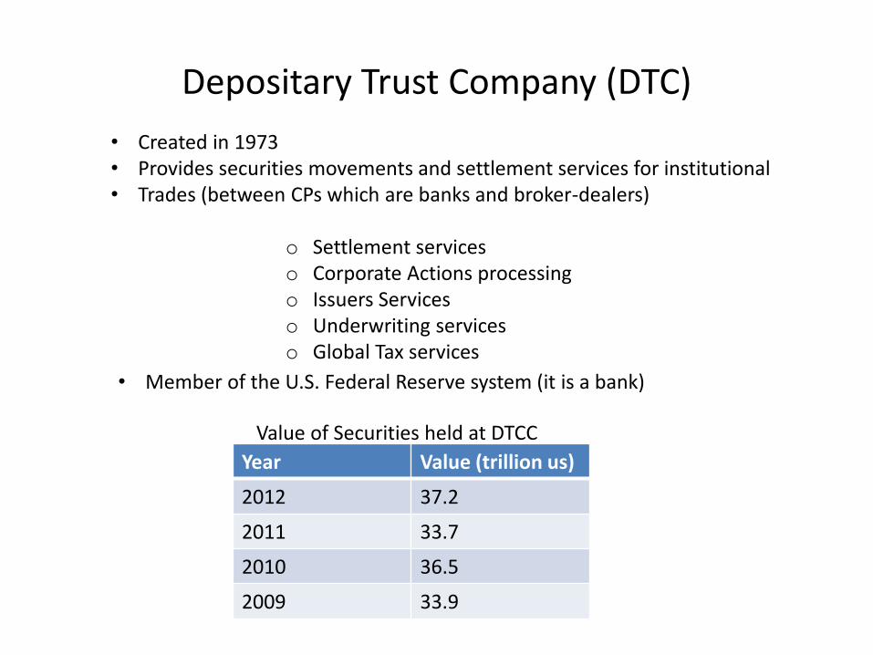
Depositary Trust Company (DTC)

• Created in 1973 • Provides securities movements and settlement services for institutional• Trades (between CPs which are banks and broker-dealers)

o Settlement serviceso Corporate Actions processingo Issuers Serviceso Underwriting serviceso Global Tax services

• Member of the U.S. Federal Reserve system (it is a bank)

Year Value (trillion us)

2012 37.2

2011 33.7

2010 36.5

2009 33.9

Value of Securities held at DTCC

CME Clearing

• Exchange Traded Derivative Products- Futures, Options- ED, E-mini, T bonds and notes, CL, Nat Gas

• OTC Financial Derivatives

• OTC Energy Derivatives

CME Clearing

CME OTC Financial Derivatives

Product TypeMax 51

Year Maturity

Max 31 Year

Maturity

Max 30 Year

Maturity

Max 15 Year

Maturity

Max 11 Year

Maturity

Max 3 Year Maturity

Vanilla Fixed vs. FloatEUR, GBP,

USD

AUD, CAD, CHF, DKK, JPY, NOK,

SEK

HKD, NZD, SGD

CZK, HUF, MXN, PLN,

ZAR

Amortizing & Accreting Swaps (Variable Notional)

EUR, GBP, USD

AUD, CAD, CHF, DKK, JPY, NOK,

SEK

Basis SwapEUR, GBP,

USDJPY FED Funds

Zero Coupon SwapEUR, GBP,

USD

Overnight Index Swap (OIS)EUR, GBP, JPY, USD

Forward Rate Agreements (FRAs)

EUR, GBP, JPY, USD,

ZAR

FX

•Major Currencies (CLS-Eligible)

•Non-CLS Physically-Settled Currencies

•CLS-Settled Currencies

•Non-CLS Cash-Settled Currencies

Energy

•Biofuels

•Natural Gas

•Power

•Petroleum

•Emissions

Agriculture

•Fertilizer

•Cocoa

CME Exchange-Traded Products (FX, Energy)

ICE Clearing US

ICE Clear Europe

ICE Clear Credit

The BM&F Bovespa clearing system

Client

lLiListed Deriv.

OTC Deriv.

Equities,SecuritiesLending

Bonds FX

10,000 Derivatives Accounts500,000 Equities AccountsFull client segregation model – all accounts are subject to BM&F Bovespa margin

not just broker-dealers

collateralcollateral

collateralcollateral

The CPSS/IOSCO Principles(Bank of International Settlements, 2012, 2016)

Principles for Financial Market Infrastructures(CPSS – IOSCO 2012)

A Financial Market Infrastructure is defined as a system that facilitates the clearing, settling or recording of payments, securities, derivatives or otherfinancial transactions.

Main categories:

1. Payment systems (PS)

2. Central securities depositories (CSD)

3. Securities Settlement Systems

4. Central Counterparties (CCPs)

5. Trade Repositories (TRs)

Principles 1-3: General Organization

Provide guidance on the general organization of an FMI to help establish a strong foundation for an FMI’s risk management.

• Strong legal basis

• Robust governance arrangements that focus on the safety and efficiency of the FMI and that support the stability of the broader financial system

• Sets new standard for establishing an integrated and comprehensive view of its risks (e.g., risks to its participants)

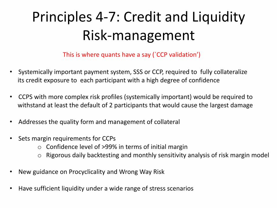
Principles 4-7: Credit and Liquidity Risk-management

• Systemically important payment system, SSS or CCP, required to fully collateralize its credit exposure to each participant with a high degree of confidence

• CCPS with more complex risk profiles (systemically important) would be required towithstand at least the default of 2 participants that would cause the largest damage

• Addresses the quality form and management of collateral

• Sets margin requirements for CCPso Confidence level of >99% in terms of initial margin o Rigorous daily backtesting and monthly sensitivity analysis of risk margin model

• New guidance on Procyclicality and Wrong Way Risk

• Have sufficient liquidity under a wide range of stress scenarios

This is where quants have a say (`CCP validation’)

Credit and Liquidity Risk Management (continued)

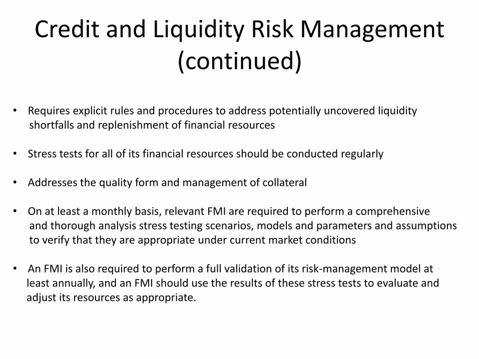
• Requires explicit rules and procedures to address potentially uncovered liquidity shortfalls and replenishment of financial resources

• Stress tests for all of its financial resources should be conducted regularly

• Addresses the quality form and management of collateral

• On at least a monthly basis, relevant FMI are required to perform a comprehensiveand thorough analysis stress testing scenarios, models and parameters and assumptionsto verify that they are appropriate under current market conditions

• An FMI is also required to perform a full validation of its risk-management model atleast annually, and an FMI should use the results of these stress tests to evaluate andadjust its resources as appropriate.

Principles 8 to 10: Settlement

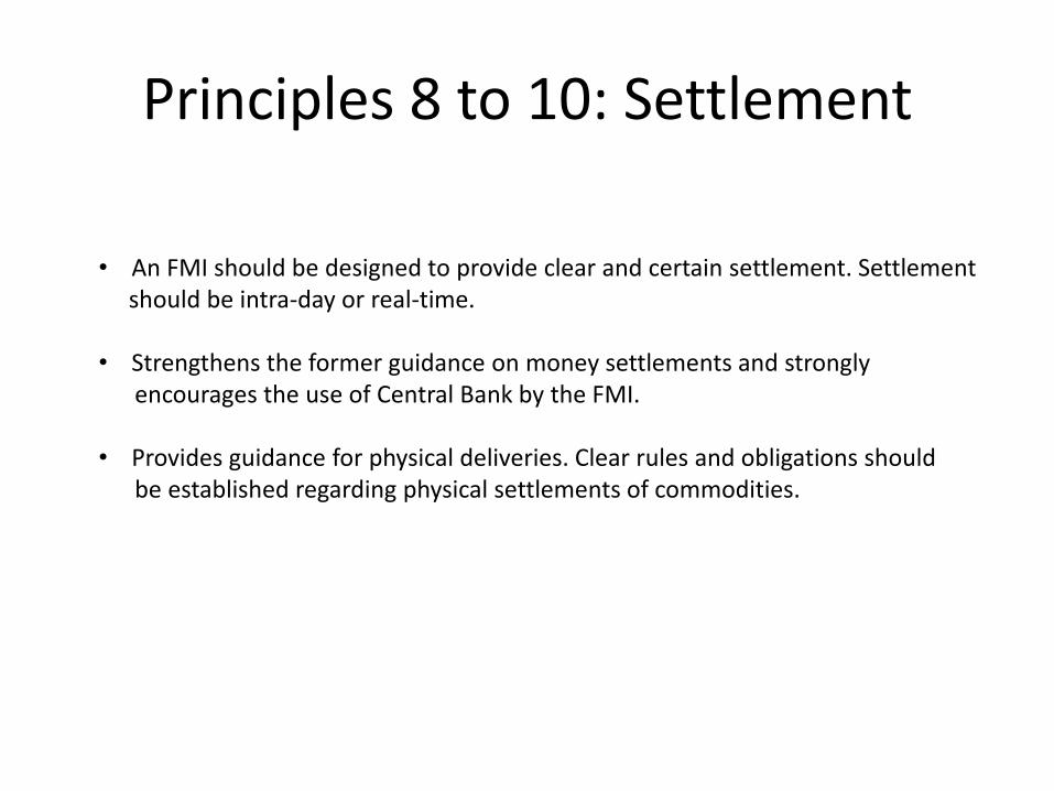
• An FMI should be designed to provide clear and certain settlement. Settlementshould be intra-day or real-time.

• Strengthens the former guidance on money settlements and strongly encourages the use of Central Bank by the FMI.

• Provides guidance for physical deliveries. Clear rules and obligations shouldbe established regarding physical settlements of commodities.

Principles 11-12: Exchange-of-value settlement

• Requires that a CDS maintain securities in an immobilized form fortransfer by book entry

• Requires elimination of principal risk by ensuring that one settlementtakes place if and only if the linked obligation is made.

13-14: Default Management

• Appropriate procedures to handle participant defaults

• Maintain rules and procedures that enable the segregation and portabilityof the position of the participant’s customers and the collateral posted

• Appropriate segregation and portability with a CCP is especially importantfor central clearing of OTC derivatives

15-17: Business and Operational Risk-Management

• FMI s required to hold liquid net assets funded by equity equal to 6 months of current operating expenses to continue operations. The funds are in addition to funds for covering CP defaults and otherrisks

• Requires an FMI to safeguard its own assets and those of its participantsand to maintain investment policies consistent with risk-management

strategy.

• Operational reliability and resilience, business continuity plans, etc.

Principles 23-24: Transparency

• Rules, key procedures and market data require sufficient disclosure byan FMI to allow participants and prospective participants to have anunderstanding of risks, fees and material cost.

• Disclosure of market data by trade repositories is a new principle specificto TRs do disclose market data and allow participants, authorities and the public to make timely assessments of the OTC derivatives markets and, if relevant, other markets served by the TR.

Case Study I:Sizing the Guarantee Fund of a CDSclearing house (2008)

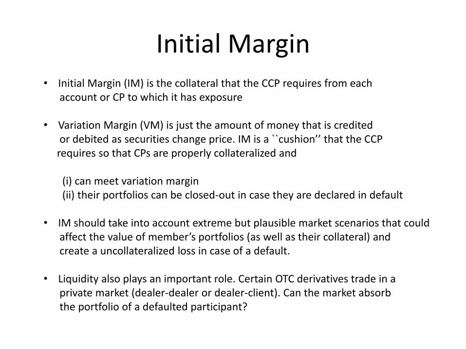
Initial Margin• Initial Margin (IM) is the collateral that the CCP requires from each

account or CP to which it has exposure

• Variation Margin (VM) is just the amount of money that is creditedor debited as securities change price. IM is a ``cushion’’ that the CCP

requires so that CPs are properly collateralized and

(i) can meet variation margin(ii) their portfolios can be closed-out in case they are declared in default

• IM should take into account extreme but plausible market scenarios that couldaffect the value of member’s portfolios (as well as their collateral) andcreate a uncollateralized loss in case of a default.

• Liquidity also plays an important role. Certain OTC derivatives trade in a private market (dealer-dealer or dealer-client). Can the market absorb the portfolio of a defaulted participant?

Guarantee Fund

• The Guarantee Fund is composed of contributions of Clearing Participantsthat should mutualize the uncollateralized losses in case of the default of market participants.

• Normally, the GF is part of a ``risk waterfall’’ which defined in the Risk Policyof the CCP

• The sizing of the Guarantee Fund and how much each clearing member shouldcontribute is key in the design of CCPs.

• The GF and other liquidity mechanisms depend on the nature of the business and, particularly, to the number of clearing participants

• Usually, clients of broker-dealers do NOT contribute to the GF, but add to the risk of the client account, which could represent more cost for the introducing broker.

Testing the size of the Guarantee Fund:The N-counterparty model

Suppose that the CCP has N counterparties, and there are n products. The ``portfolio’’ or aggregate positions of CPs can be described as a matrix

where

nNnn

N

N

QQQ

QQQ

QQQ

...

............

...

...

21

22221

11211

Q

N

j

ij

ij

niQ

ijQ

1

.,...,1 allfor 0

#product on # CPby exposure (dollar) notional

Market Risk

nXX ,...,' 1X = vector of shocks associated with a market move for the n products that are cleared (stress scenario)

We are interested in:

(a) specifying a reasonable joint probability distribution for the vector Xand looking at extreme values for the N portfolios,

(b) choosing a historical period in the past that is very volatile (e.g. Oct1987 for stocks, Sep 2008 for credit) and letting X represent the historical market move(s) over those periods.

MTM vector for the model with N clearing participants

Given a portfolio matrix Q and a market shock X, the change in the value ofthe position of the jth CP is

QX'Y

'

,...,1 ,1

NjQXY ij

n

i

ij

Margin is modeled as a function of the position. For simplicity, we can Assume that it is a linear function of the position (e.g. prop to exposure)

ij

n

i

ij QmQm

1

*

Mathematical model for simulatingCCP exposure –linear margin

ARmXZ

ARR11IQ

R

'

1

entries IIDh matrix wit random 1

1

111

1

ij

n

i

ii

ij

n

i

iij

n

i

iij

n

i

ijj

n

i

ijijij

QmX

QmQXQmYZ

n

Rn

RQ

Margin as a multiple of portfoliovariance (correlation offset)

``VaR’’ margin:

ARQ

CQeQ'e jj

,

'

11

1

*

kjij

n

ik

ikkiij

n

i

ij

kjij

n

ik

ikkij

QQmQXZ

m

QQmQm

Monte Carlo simulations: testing the margin/GF requirements of a Clearinghouse

for CDS index products

• Reference period: the week of 9/11/2008 to 9/18/2008 (defaults ofLehman Brothers)

• Data: bid-ask prices, estimates of liquidity

Steps taken:

• Code the margin requirements proposed by the architects of the clearinghouse

• Simulate 100K market configurations (portfolios) and analyze what happens inin the event that we have to liquidate two insolvent CPs . Does the clearinghouseremain solvent?

• What are the worst-case scenarios for the CCP in terms of market configurations?

Marco Avellaneda & Rama Cont, 2008/2009

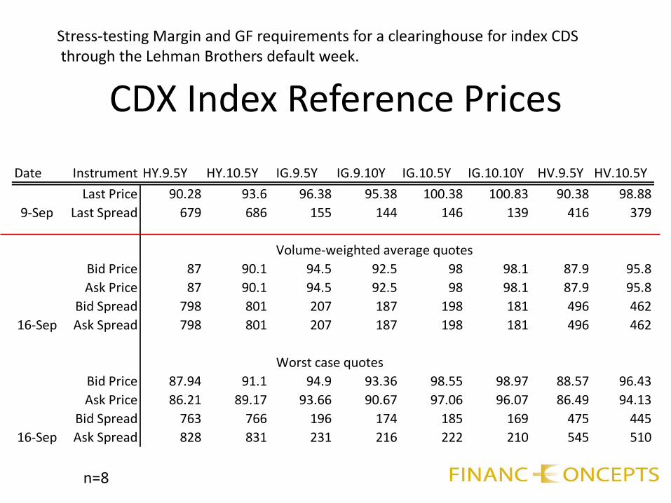
Date Instrument HY.9.5Y HY.10.5Y IG.9.5Y IG.9.10Y IG.10.5Y IG.10.10Y HV.9.5Y HV.10.5Y

Last Price 90.28 93.6 96.38 95.38 100.38 100.83 90.38 98.88

Last Spread 679 686 155 144 146 139 416 379

Volume-weighted average quotes

Bid Price 87 90.1 94.5 92.5 98 98.1 87.9 95.8

Ask Price 87 90.1 94.5 92.5 98 98.1 87.9 95.8

Bid Spread 798 801 207 187 198 181 496 462

Ask Spread 798 801 207 187 198 181 496 462

Worst case quotes

Bid Price 87.94 91.1 94.9 93.36 98.55 98.97 88.57 96.43

Ask Price 86.21 89.17 93.66 90.67 97.06 96.07 86.49 94.13

Bid Spread 763 766 196 174 185 169 475 445

Ask Spread 828 831 231 216 222 210 545 510

9-Sep

16-Sep

16-Sep

CDX Index Reference Prices

Stress-testing Margin and GF requirements for a clearinghouse for index CDSthrough the Lehman Brothers default week.

n=8

CDX Positions per firm(in millions of USD)

Firm Short Protection Long Protection Net Total Notional

CP1 16,917 1,275 (15,642) 18,192

CP2 14,497 1,605 (12,892) 16,102

CP3 13,267 1,861 (11,406) 15,128

CP4 923 17,228 16,305 18,151CP5 705 6,472 5,767 7,177

CP6 2,527 8,194 5,667 10,721

CP7 12,148 13,755 1,607 25,903

CP8 4,911 2,065 (2,846) 6,976

CP9 3,596 7,455 3,859 11,051

CP10 6,999 16,580 9,581 23,579CLEARINGHOUSE 76,490 76,490 - -

N=10 participants

Margin Requirements(in million USD)

Firm Guarantee Fund GF+Min Req Risk Margin Concentration Total Required

CP1 458.9 458.9 468.8 103.2 1,030.9

CP2 207.9 207.9 265.1 30.7 503.7

CP3 110.0 110.0 233.9 26.2 370.1

CP4 6.5 20.0 186.0 4.7 210.7

CP5 3.7 20.0 105.3 0.0 125.3

CP6 3.6 20.0 102.0 0.0 122.0

CP7 9.6 20.0 272.2 24.7 316.9

CP8 2.0 20.0 57.9 2.7 80.6

CP9 4.0 20.0 113.1 0.0 133.1

CP10 12.4 20.0 353.3 51.1 424.4

CLEARINGHOUSE 818.6 916.7 2,157.6 243.3 3,074.4

Estimated Profit/Loss:Liquidation on Sep 16, 2008

Volume-weighted average quote

Worst-case quote on Sep 16

Firm HY.9.5Y HY.10.5Y IG.9.5Y IG.9.10Y IG.10.5Y IG.10.10Y HV.9.5Y HV.10.5Y Total

CP7 68.4 100.2 (158.7) (81.4) 177.8 (24.0) 28.4 5.9 116.6

CP2 52.6 (71.0) (14.4) (61.4) (121.8) (68.4) (14.0) (42.5) (340.9)

CP1 27.8 (277.7) (10.1) (80.4) (71.2) (44.2) (25.9) 13.2 (468.5)

Firm HY.9.5Y HY.10.5Y IG.9.5Y IG.9.10Y IG.10.5Y IG.10.10Y HV.9.5Y HV.10.5Y Total

CP7 48.8 71.6 (229.7) (133.1) 136.7 (41.8) 20.7 4.7 (122.1)

CP2 37.6 (89.8) (20.9) (100.5) (169.9) (119.3) (22.0) (65.6) (550.4)

CP1 19.8 (351.5) (14.6) (131.6) (99.3) (77.1) (40.7) 10.5 (684.3)

Comparing Shortfalls withClearinghouse requirements

Worst-case quote on Sep 16

Firm Worst Case Total Req. Risk Marg. Concentration Guarantee Fund

CP7 (122.1) 316.9 272.2 24.7 20.0

CP2 (550.4) 503.7 265.1 30.7 207.9

CP1 (684.3) 1,030.9 468.8 103.2 458.9

Comparing Shortfalls withClearinghouse requirements

Volume-weighted average quote

Firm VWAQ Total Req. Risk Marg. Concentration Guarantee Fund

CP7 116.6 316.9 272.2 24.7 20.0

CP2 (340.9) 503.7 265.1 30.7 207.9

CP1 (468.5) 1,030.9 468.8 103.2 458.9

Firm positions on September 16 (notional in USD millions)

Firm HY.9.5Y HY.10.5Y IG.9.5Y IG.9.10Y IG.10.5Y IG.10.10Y HV.9.5Y HV.10.5Y

CP7 2,084 2,864 (8,444) (2,825) 7,472 (879) 1,145 190

CP2 1,605 (2,028) (767) (2,133) (5,116) (2,506) (566) (1,381)

CP1 847 (7,934) (535) (2,793) (2,991) (1,619) (1,045) 428

Simulating different portfolios

houses clearingby proposed rules GF andMargin

2008 18, Sep11/ Sep of week over the prices toShocks

Dbillion US 7by bounded , )protectionshort or (long entries ddistribute Uniformly

CDSindex NA in dealersprimary ,10

years 10 years, 5 ,.,.,. 8

X

R

N

IGCDXHVCDXHYCDXn

Objective: explore the ``phase space’’ of all possible portfolios that couldexist in this period and find hw and why extreme losses could happen.

Simulated losses for CCP in case of liquidationof 2 insolvent CPs

( % of Total Guarantee Fund)

Freq

ue

ncy

Shortfall as % of total GF,after applying GF of each CP

Effects of netting the positions of 2 insolvent CPs

If two or more participants must be liquidated, offsetting positions can be cancelled out. This is known as netting.

Case Study II:Monte Carlo RM system for ExchangeTraded Equity Options CCP:The Options Clearing Corporation(2013)

60

U.S. Equity Derivatives in Numbers

• Number of underlying securities with options (Stocks, Indices, ETFs) : ~ 9,000

• Number of Open contracts per underlying asset: ~ 100 (average)

• Total number of open contracts on a given day: ~ 1,000,000

• Professional trading firms position size ~ 25,000+ positions

• Size of Daily Mark-to-Market: 60 MB compressed zip file

• 5 Years historical MTM : 75 GB

• Commercial data vendors: Hanweck Option Volatility Service, IVY OptionMetrics

• Intraday data: orders of magnitude larger!

61

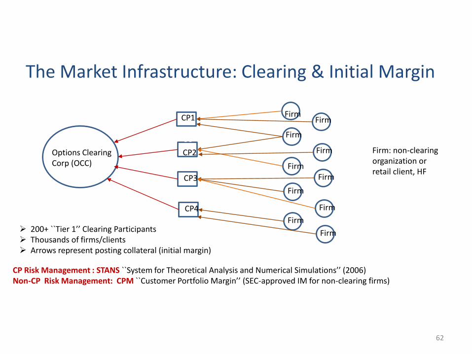
The Market Infrastructure: Clearing & Initial Margin

CCP2C

Options ClearingCorp (OCC)

CP1

CP2

CP3

CP4

FirmFirm

Firm

Firm

FirmFirm

Firm

Firm

Firm

Firm

CP Risk Management : STANS ``System for Theoretical Analysis and Numerical Simulations’’ (2006)Non-CP Risk Management: CPM ``Customer Portfolio Margin’’ (SEC-approved IM for non-clearing firms)

Firm: non-clearingorganization orretail client, HF

200+ ``Tier 1’’ Clearing Participants Thousands of firms/clients Arrows represent posting collateral (initial margin)

62

Customer Portfolio Margin(FINRA rule 4210)

• Apply stress tests or `slides’ by using mathematical formulas to create new market values for positions based on theoretical movements of the underlying stock

• Move the price of the underlier by between +6% and -8% at 10 equal intervals (grid) for broad indexes

• Move by +15% and -15% for ETF, equities

• Add worst losses for each separate underlying stock & options to obtain CPM requirement

• CPs must use an SEC/FINRA approved model to margin their clients (minimum requirement)

• Currently, the Option Clearing Corporation’s TIMS is the only approved model for CPM

CPM/TIMS is very rigid, does not recognize any correlations except for Broad-Based Indexes.(Basically, it’s a 1980’s approach).

Reference: http://www.optionsclearing.com/risk-management/cpm/

63

STANS: Initial Margin For CPs (2006)• Grids are replaced by a Monte Carlo Simulation for 2-day changes in all (correlated) underlying prices

• Amplitudes of moves based on estimated Standard Deviations, correlations between underlying stockstaken into account via MC

• Portfolios re-priced 10,000 times using 10,000 theoretical changes of the underlying stocks based on MC.

𝐵𝑎𝑠𝑒 𝐶ℎ𝑎𝑟𝑔𝑒 = 𝐸𝑆99%

𝐷𝑒𝑝𝑒𝑛𝑑𝑒𝑛𝑐𝑒 𝐶ℎ𝑎𝑟𝑔𝑒 = 0.25 × max 𝐸𝑆99.5%𝐻 , 𝐸𝑆99.5%

𝜌=1, 𝐸𝑆99.5%

𝜌=0− 𝐸𝑆99%

𝐶𝑜𝑛𝑐𝑒𝑛𝑡𝑟𝑎𝑡𝑖𝑜𝑛 𝐶ℎ𝑎𝑟𝑔𝑒 = 0.25 ×2𝑐𝐸𝑆99.5% +2 𝑟𝐸𝑆99.5% − 𝐸𝑆99% (Worst 2-asset portfolio)

𝑆𝑇𝐴𝑁𝑆 𝐼𝑀 = 𝐵𝑎𝑠𝑒 𝐶ℎ𝑎𝑟𝑔𝑒 + 𝐷𝑒𝑝𝑒𝑛𝑑𝑒𝑛𝑐𝑒 𝐶ℎ𝑎𝑟𝑔𝑒 + 𝐶𝑜𝑛𝑐𝑒𝑛𝑡𝑟𝑎𝑡𝑖𝑜𝑛 𝐶ℎ𝑎𝑟𝑔𝑒

http://www.optionsclearing.com/risk-management/margins/

(Correlations scenarios)

(Expected shortfall @ 99%)

Expected Shortfall (ES) • Given 𝑁 = 10,000 scenarios for theoretical portfolio changes: 𝑋1<𝑋2 < 𝑋3 < ⋯ < 𝑋𝑁

• ES is better than Value at Risk because it takes into account tail riskbeyond VaR

𝐸𝑆𝛼 =1

𝑁(1 − 𝛼)

𝑖=1

𝑁(1−𝛼)

𝑋𝑖 𝛼 = 99%, 99.5%

Var 99%

ES= average worst 1% pnl

65

Improving STANS (2013-2016) • STANS ``scenarios’’ only take into account changes in the underlying asset

• STANS does not shock the implied volatility (IVOL) of the options

STANS (2006): 𝐵𝑆 𝑆, 𝑇, 𝐾, 𝜎 → 𝐵𝑆 𝑆 + ∆𝑆, 𝑇, 𝐾, 𝜎

NEW STANS (2016): 𝐵𝑆 𝑆, 𝑇, 𝐾, 𝜎 → 𝐵𝑆 𝑆 + ∆𝑆, 𝑇, 𝐾, 𝜎 + ∆𝜎

• Motivation: For longer-dated options, IVOL risk can be more important than underlying stock risk• Futures and ETFs referencing the VIX volatility index blur the boundary

between what is an underlying asset and what is an implied volatility.

• M. A. and Finance Concepts LLC advised the OCC in creating the improved STANS (2016)

• Improved STANS was recently approved by SEC

66

`frozen IVOL’

67

New STANS (SEC Filing)

http://www.optionsclearing.com/components/docs/legal/rules_and_bylaws/sr_occ_15_804.pdf

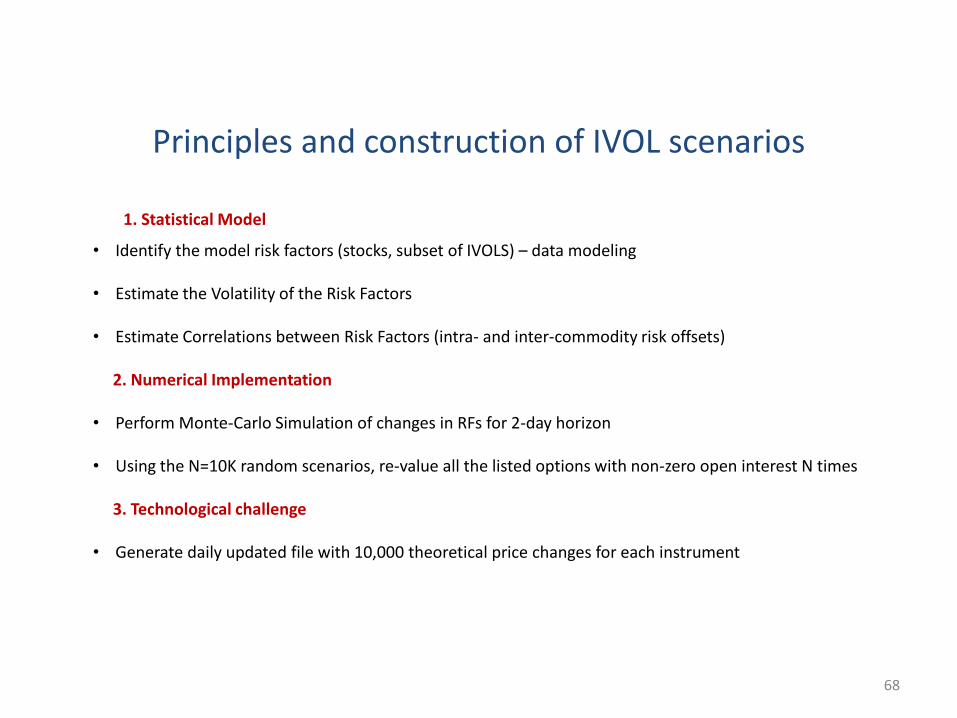
Principles and construction of IVOL scenarios

68

• Identify the model risk factors (stocks, subset of IVOLS) – data modeling

• Estimate the Volatility of the Risk Factors

• Estimate Correlations between Risk Factors (intra- and inter-commodity risk offsets)

2. Numerical Implementation

• Perform Monte-Carlo Simulation of changes in RFs for 2-day horizon

• Using the N=10K random scenarios, re-value all the listed options with non-zero open interest N times

3. Technological challenge

• Generate daily updated file with 10,000 theoretical price changes for each instrument

1. Statistical Model

Statistical Model

69

• How can we parametrize the options market for a given underlying asset?

Answer : Build an ``implied volatility surface’’ for each asset

• How can we parametrize the implied volatility surface with the ``right’’ number of degrees of freedom

Answer: Use principal components analysis on the correlation matrix of IVOLs for each asset tofind a minimal set of risk factors

Academic study (M.A., Doris Dobi, & Finance Concepts)

• Data source: IVY OptionMetrics (available at WRDS for colleges), which givesEOD prices from OPRA

• Study: consider 4,000 optionable securities with 52 delta-maturity pointsper underlying asset + underlying asset (53 points per asset)

• Use smoothing of implied volatilities of options to generate a constant-maturity,constant-moneyness dataset for each day:

𝛿 = 20,25,30,… , 75,80,100 , 𝜏=(30,91,182, 365)BS Delta (13 strikes) 4 settlement dates

• Historical period: August 31, 2004 to August 31, 2013

http://www.math.nyu.edu/faculty/avellane/DorisDobiThesis.pdf

Correlation Analysis for Stock and IVOL surface

• For each underlying stock, ETF or index, we formed the matrix

𝑿𝒕,𝒊 = standardized returns of stock (i=1) or of the IVOL surface point labeled i

• Perform an SVD of the volatility surface for each of the underlying assetsin the dataset.

• Analyze eigenvectors and eigenvalues to find out how correlated IVOLS arefor a given underlying asset

𝑋 =

𝑋1,1 ⋯ 𝑋1,53⋮ ⋱ ⋮

𝑋𝑇,1 ⋯ 𝑋𝑇,53

T=1257 (5 years history)

Principal Component Analysis of the IVOL Correlation matrix: separating signal from noise

• Question: how many significant eigenvalues/eigenvectors do the correlation matricesof implied volatilities have?

• Random matrix theory: if X is a matrix of uncorrelated IID random variables withmean zero and variance 1, of dimensions 𝑇 × 𝑁, the histogram of the eigenvalues of the

correlation matrix

approaches, as N and T tend to infinity with ratio N/T=𝛾, the Marcenko-Pasturdistribution:

𝐶 =1

𝑇𝑋𝑋′

# 𝜆: 𝜆 ≤ 𝑥

𝑁→ 𝑀𝑃 𝛾; 𝑥 =

0

𝑥

𝑓 𝛾; 𝑦 𝑑𝑦

N → ∞,𝑁

𝑇→ 𝛾

Marcenko-Pastur distribution & threshold

𝑓 𝛾; 𝑥 = 1 −1

𝛾

+

𝛿 𝑥 +1

2𝜋𝛾

𝑥 − 𝜆− 𝜆+ − 𝑥

𝑥𝜆− ≤ 𝑥 ≤ 𝜆+

𝜆− = 1 − 𝛾 2 𝜆+ = 1 + 𝛾 + Marcenko-Pasturthreshold

The theoretical top EV for N=53 and T=1250 is 𝜆+ = 1 +53

1257

2

= 1.45

Assumption: Eigenvalues of the correlation matrix associated with non-random featuresshould lie above the MP threshold (within error; Laloux, et al (2000),Bouchaud and Potters (2000))

Analysis of SPX volatility surface

Stock down

Vol up95%

2 × 2%

Spectrum First eigenvector

Third eigenvectorSecond eigenvector

MP threshold= 1.45

1 significant eigenvalue(out of 53 possible)

Lambda_1 50.04

Lambda_2 1.3

Lambda_3 0.93

Number of EVs above the MP threshold for all optionable assets

Small stocks/ takeovers/ idiosyncratic namesWell-known/ broadly

traded namesSPX

Dimension reduction

• Knowing that DF<=9, from PCA, choose a small set of points on the IVSand their fluctuations to model the changes in implied volatilitiesfor each underlying.

• A pivot is a point on the delta/tenor surface used as a risk factor

• A pivot scheme: is a grid of pivots, which will be used to interpolate theimplied volatility returns.

• Goal: find a pivot scheme that approximates well movements of the full volatility surface

Example: 9-pivot scheme interpolates IVOL shocks from a discrete set of 9

moves

The change in the IVOL at this pointis the linear interpolation of the changes

for the 4 surrounding pivots

Day

s to

mat

uri

ty

BS Call Delta

78

75 delta 50 delta 25 delta

30

91

182

365

75 delta 50 delta 25 delta

30

91

182

365

75 delta 50 delta 25 delta

30

91

182

365

2 pivots 4 pivots 5 pivots

6 pivots 7 pivots 75 delta 50 delta 25 delta

30

91

182

365

9 pivots 75 delta 50 delta 25 delta

30

91

182

365

12 pivots

Some of the pivot schemes that were tested

75 delta 50 delta 25 delta

30

91

182

365

75 delta 50 delta 25 delta

30

91

182

365

Increasing the number of pivots results in a better approximation of EV1

2 pivots 6 pivots

9 pivots

Cross section of S&P 500 constituents.

% Error

12- pivot scheme does slightly better, but notmuch better, than 9 pivots

9 pivots 12 pivots

• 9 pivots seems like an appropriate number to parameterize all the IVS in the data.

• This was confirmed by dynamic PCA with smaller window (Dobi’s thesis, 2014)

• Also confirmed by backtesting initial margin on many test portfolios (tail risk)

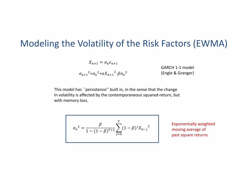
Modeling the Volatility of the Risk Factors (EWMA)

𝑋𝑛+1 = 𝜎𝑛𝜖𝑛+1

𝜎𝑛+12=𝜎𝑛

2+𝛼𝑋𝑛+12-𝛽𝜎𝑛

2

GARCH 1-1 model(Engle & Granger)

This model has ``persistence’’ built in, in the sense that the changeIn volatility is affected by the contemporaneous squared-return, but with memory loss.

𝜎𝑛2 =

𝛽

1 − (1 − 𝛽)𝑇+1

𝑗=0

𝑇

(1 − 𝛽)𝑗𝑋𝑛−𝑗2

Exponentially weightedmoving average ofpast square returns

Putting the model together (inter-commodity correlations)

• We determined that for each equity and its listed options, the 9-pivotmodel is sufficient to describe statistically the changes in the entire market

• Use this information to estimate the joint correlation matrix of all stocks/IVOLSin the DB.

• Experiment: We study 3141 equities over 500 days. The dimensionality in column space (number of risk-factors) is N~ 3,000× 10 = 30,000. The number of rows is 500.

• We have to model a correlation matrix of roughly 30K × 30K.

• Idea: Perform PCA on the full correlation matrix of all ``pivot returns’’ (30,000). Extractsignificant eigenvalues and eigenvectors

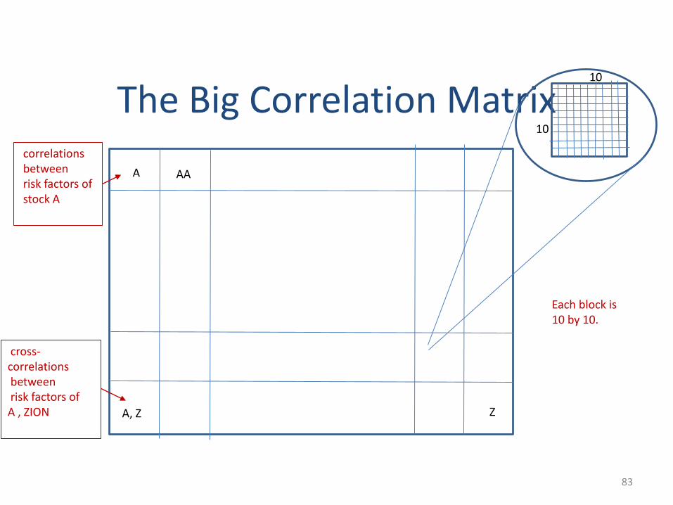
The Big Correlation Matrix

83

10

10

A AA

ZA, Z

correlationsbetween risk factors of stock A

cross-correlationsbetween risk factors of A , ZION

Each block is 10 by 10.

Marcenko-Pastur Analysis for Big Matrix

• The MP Threshold is

• This suggests that we keep eigenvalues above 79.67 and declare thatthe rest is noise….

• Question : how many EVs exceed (significantly) the threshold level 79.67?

𝜆+ ≈ 1 +31410

500

2

= 79.67

Answer: There are ~ 108 significant Evs in the options market

MP threshold

Numerically, this implies that we need to calculate only the top 108 eigenvalues/eigenvectors of the `raw’ correlation matrix.

Monte Carlo Simulation*

86

𝑋 = Σ 𝑅1/2Z

Where

𝑋 = vector of changes in all risk-factors (N_underlyings × 10)

Σ = diagonal matrix of estimated EWMA standard deviations (2-day changes)

𝑅1/2= square-root of the estimated correlation matrix of X (SVD, 108 top eigenvalues)

Z = vector of standardized uncorrelated random variables with suitable probability distributions(heavy tails)

* Slightly simplified for this presentation.

10,000 random draws of Z give rise to the 10,000 scenarios for risk factors

Numerical Linear Algebra

• Our first calculations of spectra and eigenvalues for the Big Correlation Matrixwere hopelessly slow.

• Storage issues (get more RAM!)

• SVD calculations without care are 𝑂 𝑁3 where 𝑁 is the number of factors

• Fortunately, a series of techniques used by Data Mining and Big Data scientistscan be applied to reduce computational times dramatically

• Idea: sample the column data and the row data randomly or pre-multiply databy a random matrix.

Fast SVD, low rank approximations

Let A be a ``data matrix’’: m rows, n columns

We look for a good rank k approximation of A, where k<<n:

The best rank k approximation uses the top k eigenvectors of the matrix 𝐴𝐴𝑇.(The approximation is in the sense of the L2 norm for matrices. )

Rokhlin, Zlam, and Tygert, 2009

• For SVD, approximate the optimal rank-k approximation by multiplying the data by a random 𝑛 × 𝑘 matrix, G (i.i.d. Uniform(0,1)), and performing SVD

→

A G A×

• Pre-multiplying has the effect of sampling the data (our interpretation) andpreserves the correlation matrix of the market. The advantage is that

we work with a much smaller matrix.

• Using appropriate choice of k, according to the rank of m (108) , leads tovery small errors in the spectrum. (Hence accurate reconstruction oftrue correlation).

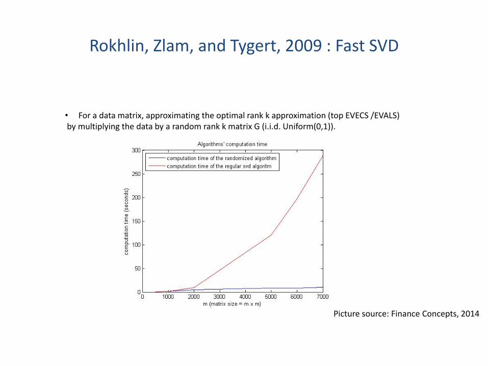
Rokhlin, Zlam, and Tygert, 2009 : Fast SVD

• For a data matrix, approximating the optimal rank k approximation (top EVECS /EVALS)by multiplying the data by a random rank k matrix G (i.i.d. Uniform(0,1)).

Picture source: Finance Concepts, 2014

All available stocks in OptionMetrics +pivots

Data size: N=31,837, k=500Computational time, randomized SVD=41 secsComputational time, regular SVD = too long to observe

For comparison purposes, we also did a 20,000 risk factor matrix.Data size: N=20,000, k=500Computational time, randomized SVD=17 secsComputational time, regular SVD = 4520 secs

Comparison of approximateand actual evs for the top 500Eigenvalues give very small errors of order10−28 − 10−23

Source: Finance Concepts, 2014

Numerical implementation issues

92

• Due to fast SVD algorithm, the computation of the square-root of the correlation matrix is very fast.

The main bottlenecks are:

• Computing the initial 9-pivots for each surface from closing data

• Repricing all the options with BS under the 10,000 risk scenarios ( 10 billion BS calculations)

Spread risk

Correlation Risk

Jump-to-default risk

Jump-to-health risk

Liquidity risk*

Interest rate risk*

Case Study III:Monte-Carlo Framework for Margining Credit Default Swaps (OTC derivatives CCP)(2013/2014)

94

Description of the Model : Single Name CDS and CDS

Index Factors

Risk-factors are spreads’ log changes

• Single Name CDS : Par spreads at fixed benchmark tenors (1, 3, 5, 7, 10 years)

• CDS Indices : Par spreads of synthetic OTR-k (k=0,1,…) indices (fixed maturity)

interpolated at fixed benchmark tenors to preserve stationarity

Salient characteristics of risk factors

• Autocorrelations : non-uniform across entities and tenors

• Heteroscedasticity

• Varying degrees of heavy tails : observed, but statistically weak asymmetry

• Stable average correlations

- Single name – Single name

- Single name – Index

- Index – Index

• Strong correlations across tenors

• Strong dependence across on-the-run and off-the-run indices (same index family)

• Index – constituent basis

• Breakdown of correlations in distressed markets

• Jumps: defaults and drastic improvements in credit quality

95

Autoregressive and Heteroscedastic Nature of Risk-

factor distributions

For a given tenor 𝜏 and name 𝑖 (SN or Index):

𝑅𝑖,𝜏 𝑡 = 𝑎𝑖,𝜏 𝑡 𝑅𝑖,𝜏 𝑡 − 1 + 𝜎𝑖,𝜏 𝑡 휀𝑖,𝜏 𝑡

𝑅𝑖 𝑘, 𝑡 is a daily log-return of the risk factor par spreads

𝑅𝑖,𝜏 𝑡 = ln 𝐶𝐷𝑆𝑖,𝜏(𝑡) − ln 𝐶𝐷𝑆𝑖,𝜏(𝑡 − 1)

𝑎𝑖,𝜏 𝑡 is an autoregressive AR(1) coefficient for the autocorrelation observed in 𝑅𝑖,𝜏 𝑡

𝑎𝑖,𝜏 𝑡 =1

756

𝑠=1

756

𝑅𝑖,𝜏 𝑡 − 𝑠 + 1 ∗ 𝑅𝑖,𝜏 𝑡 − 𝑠

𝜎𝑖,𝜏 𝑡 is a volatility scale factor, defined as the EWMA standard deviation of the

residuals of AR(1) model

𝜎𝑖,𝜏 𝑡 =1

𝑠=1252 𝜆𝑠−1

𝑠=1

252

𝜆𝑠−1 𝑋𝑖,𝜏 𝑡 − 𝑠2

where 𝑋𝑖,𝜏 𝑡 is the deautocorrelated daily log-return : 𝑋𝑖,𝜏 𝑡 = 𝑅𝑖,𝜏(𝑡) − 𝑎𝑖,𝜏 𝑡 𝑅𝑖,𝜏(𝑡 − 1)

AR-1

96

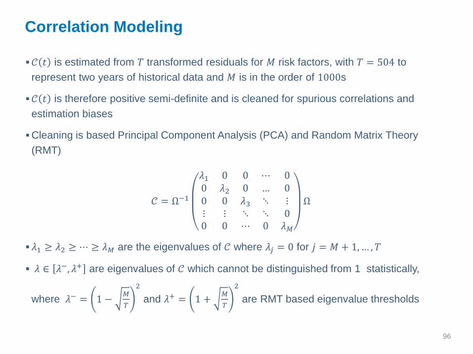
Correlation Modeling

𝒞 𝑡 is estimated from 𝑇 transformed residuals for 𝑀 risk factors, with 𝑇 = 504 to

represent two years of historical data and 𝑀 is in the order of 1000s

𝒞 𝑡 is therefore positive semi-definite and is cleaned for spurious correlations and

estimation biases

Cleaning is based Principal Component Analysis (PCA) and Random Matrix Theory

(RMT)

𝒞 = Ω−1

𝜆1 0 0 ⋯ 00 𝜆2 0 … 00 0 𝜆3 ⋱ ⋮⋮ ⋮ ⋱ ⋱ 00 0 ⋯ 0 𝜆𝑀

Ω

𝜆1 ≥ 𝜆2 ≥ ⋯ ≥ 𝜆𝑀 are the eigenvalues of 𝒞 where 𝜆𝑗 = 0 for 𝑗 = 𝑀 + 1,… , 𝑇

𝜆 ∈ 𝜆−, 𝜆+ are eigenvalues of 𝒞 which cannot be distinguished from 1 statistically,

where 𝜆− = 1 −𝑀

𝑇

2

and 𝜆+ = 1 +𝑀

𝑇

2

are RMT based eigenvalue thresholds

97

Extreme (``stressed’’) Correlations Scenarios

𝜎𝑖,𝜏 𝑡 is a long-run volatility component which introduces countercyclicality in individual

risk factor variations :

𝜎𝑖,𝜏 𝑡 =1

𝑁𝑖,𝜏(𝑡)

𝑠=0

𝑁𝑖,𝜏(𝑡)−1

𝑅𝑖,𝜏 𝑡 − 𝑠 2

𝑎𝑖,𝜏 𝑡 =1

𝑁𝑖,𝜏−1 𝑠=1

𝑁𝑖,𝜏−1𝑅𝑖,𝜏 𝑡 − 𝑠 + 1 ∗ 𝑅𝑖,𝜏 𝑡 − 𝑠 is a long-run autocorrelation estimate

which introduces countercyclicality for scaling daily volatility to margin period of risk

𝒞𝑙𝑜𝑤and 𝒞ℎ𝑖𝑔ℎ

are two correlation matrices which add countercyclicality to modeling of

the joint movement of risk factors

𝒞𝑙𝑜𝑤 =

1 0 0 0 0 00 ⋱ ⋱ ⋱ ⋱ ⋱0 ⋱ 1 ⋱ ⋱ ⋱0 ⋱ ⋱ 1 𝜌𝐼,𝐼 𝜌𝐼,𝐼0 ⋱ ⋱ 𝜌𝐼,𝐼 ⋱ ⋱

0 ⋱ ⋱ 𝜌𝐼,𝐼 ⋱ 1

and 𝒞ℎ𝑖𝑔ℎ

=

1 1 1 1 11 ⋱ ⋱ ⋱ ⋱1 ⋱ ⋱ ⋱ ⋱1 ⋱ ⋱ ⋱ ⋱1 ⋱ ⋱ ⋱ ⋱

98

Modeling the joint distribution of all risk factors

Each risk factor is modeled as a symmetric t-distribution with 𝜐𝑖,𝜏 degrees of freedom

The degree of freedom parameter is estimated by minimizing the Anderson-Darling

statistic for the conditional residuals: 휀𝑖,𝜏 𝑡 =𝑋𝑖,𝜏 𝑡

𝜎𝑖,𝜏 𝑡

𝐴𝐷𝑖,𝜏 𝜈, 𝑡

= −𝑁𝑖,𝜏 𝑡 −

𝑗=1

𝑁𝑖,𝜏 𝑡2𝑗 − 1

𝑁𝑖,𝜏 𝑡ln 𝑡𝜈

𝜈

𝜈 − 2

휀𝑖,𝜏[𝑗] − 𝜇(휀𝑖,𝜏).𝑠𝑡𝑑(휀𝑖,𝜏)

+ ln 1 − 𝑡𝜈𝜈

𝜈 − 2

휀𝑖,𝜏[𝑗] − 𝜇(휀𝑖,𝜏).𝑠𝑡𝑑(휀𝑖,𝜏)

𝜈𝑖,𝜏(𝑡) = argmin𝜈

𝐴𝐷𝑖,𝜏 𝜈, 𝑡

where 𝑁𝑖,𝜏 𝑡 is the number of all historical data available for risk factor (𝑖, 𝜏) at time 𝑡

휀𝑖,𝜏[𝑗] are the ordered conditional residuals

In the t-copula model, the correlation matrix estimate 𝒞 𝑡 is the correlation matrix of

transformed conditional residuals

𝜖𝑖,𝜏 𝑡 = 𝑡𝜈𝐶−1

𝑡 𝜈𝑖,𝜏(𝑡) 𝜈𝑖,𝜏(𝑡)

𝜈𝑖,𝜏(𝑡) − 2휀𝑖,𝜏 𝑡

99

Scenario Generation

For each Monte Carlo scenario 𝑗 = 1,… , 𝑁𝑀𝐶 , the spread shock to a given tenor 𝜏 of

name 𝑖 (SN or Index) is given by

𝑅𝑖,𝜏(𝑗) 𝑡 + 𝑛 = 𝜎𝑖,𝜏 𝑡 + 1 ⋁ 𝜎𝑖,𝜏 𝑡 𝑛 + 2(𝑛 − 1) 𝑎𝑖,𝜏 𝑡 ⋁ 𝑎𝑖,𝜏 𝑡 ⋁0 𝜉𝑖,𝜏

(𝑗)

where

• 𝜉𝑖,𝜏(𝑗)~

𝜈𝑖,𝜏−𝟐

𝜈𝑖,𝜏𝒕 𝜈𝑖,𝜏

−𝟏 Rank 𝑧𝑖,𝜏(𝑗)

where 𝑧𝑖,𝜏(𝑗)

~𝒕𝜈𝑐(𝒞) is a simulated multivariate

Student-t variable with correlation matrix 𝒞 and a common degree of freedom of 𝑡𝜈𝐶

• 𝜎𝑖,𝜏 𝑡 + 1 is the EWMA volatility forecast at margin/stress date 𝑡

- For margin calculations : 𝜎𝑖,𝜏 𝑡 + 1 = 𝜎𝑖,𝜏 𝑡 + 1

- For stress calculations : 𝜎𝑖,𝜏 𝑡 + 1 = max𝑠≤𝑡

𝜎𝑖,𝜏 𝑠 + 1

• 𝒞 is set to 𝒞0 𝑡 , 𝒞𝑙𝑜𝑤 and 𝒞ℎ𝑖𝑔ℎ

for base, basis and systematic margin requirement

calculations, respectively

• 𝜈𝑐 = 3 and 𝑁𝑀𝐶 = 10,000

100

Non-Uniform Autocorrelations Across Obligors, Tenors:

2013/6/21

0

10

20

30

40

50

Fre

qu

en

cy o

f S

ing

le N

am

es

Autocorrelation bins

Single Names (138 entities) : 1 Year

0

10

20

30

40

50

Fre

qu

en

cy o

f S

ing

le N

am

es

Autocorrelation bins

Single Names (138 entities) : 5 Year

(0.05)

-

0.05

0.10

0.15

0.20

0.25

0 5 10 15

Au

toco

rrela

tio

n

Synthetic Tenor

OTR Index

IG HY

-

0.05

0.10

0.15

0.20

0.25

0 5 10 15

Au

toco

rrela

tio

n

Synthetic Tenor

OTR-2 Index

IG HY

101

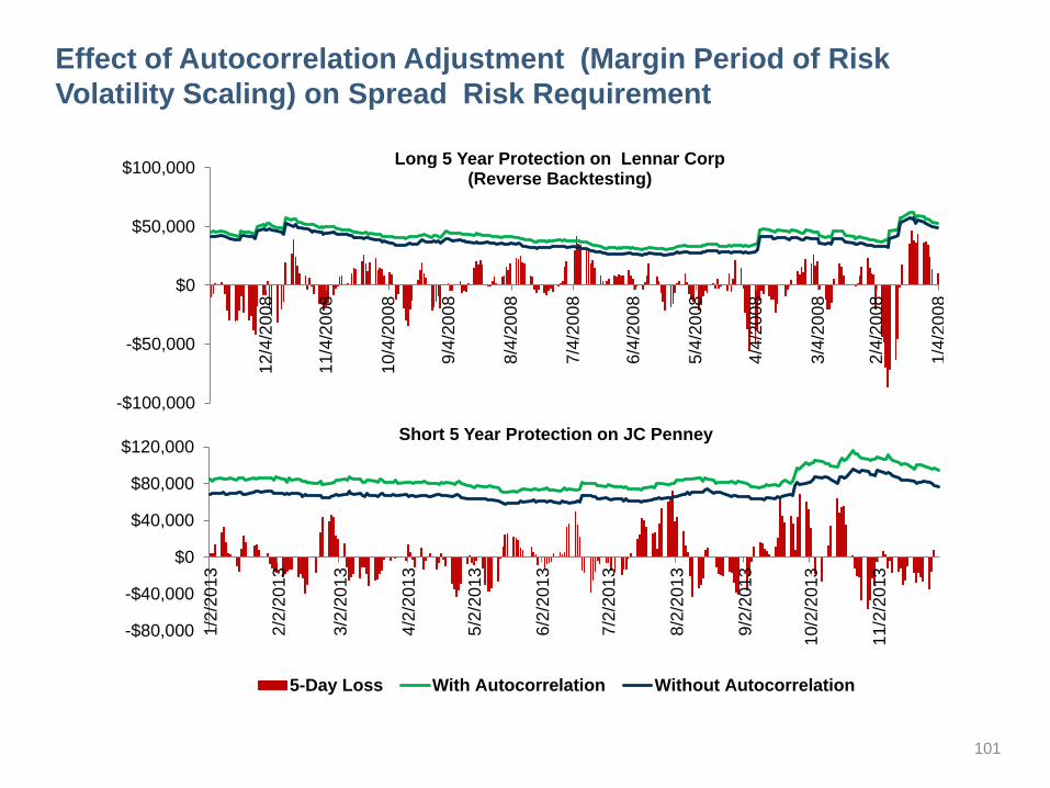
Effect of Autocorrelation Adjustment (Margin Period of Risk

Volatility Scaling) on Spread Risk Requirement

-$100,000

-$50,000

$0

$50,000

$100,000

1/4

/20

08

2/4

/20

08

3/4

/20

08

4/4

/20

08

5/4

/20

08

6/4

/20

08

7/4

/20

08

8/4

/20

08

9/4

/20

08

10/4

/20

08

11/4

/20

08

12/4

/20

08

Long 5 Year Protection on Lennar Corp(Reverse Backtesting)

-$80,000

-$40,000

$0

$40,000

$80,000

$120,000

1/2

/20

13

2/2

/20

13

3/2

/20

13

4/2

/20

13

5/2

/20

13

6/2

/20

13

7/2

/20

13

8/2

/20

13

9/2

/20

13

10/2

/20

13

11/2

/20

13

Short 5 Year Protection on JC Penney

5-Day Loss With Autocorrelation Without Autocorrelation

102

Effect of Autocorrelation Adjustment (Margin Period of Risk

Volatility Scaling) on Spread Risk Requirement

-$10,000

$0

$10,000

$20,000

$30,000

$40,000

1/4

/2008

2/4

/200

8

3/4

/200

8

4/4

/200

8

5/4

/200

8

6/4

/200

8

7/4

/200

8

8/4

/200

8

9/4

/2008

10/4

/20

08

11/4

/20

08

12/4

/20

08

Short 10 Year / Long 5 Year Protection on Anadarko Petroleum Corp :SDV01 Neutral(Reverse Backtesting)

-$9,000

-$6,000

-$3,000

$0

$3,000

$6,000

$9,000

$12,000

1/2

/201

3

2/2

/201

3

3/2

/201

3

4/2

/201

3

5/2

/201

3

6/2

/201

3

7/2

/201

3

8/2

/201

3

9/2

/201

3

10/2

/20

13

11/2

/20

13

Long 10 Year / Short 5 Year Protection on Anadarko Petroleum Corp : DV01 Neutral

5-Day Loss With Autocorrelation Without Autocorrelation

103

Heteroscedasticity, EWMA Estimate of Volatility and EWMA Mean

Absolute Deviation (MAD)

0

0.001

0.002

0.003

0

0.01

0.02

0.03

0.04

0.05

Jun-1

1

Sep-1

1

De

c-1

1

Ma

r-1

2

Jun-1

2

Sep-1

2

De

c-1

2

Ma

r-1

3

Jun-1

3

IG OTR 5 Year

Squared Returns EWMA Volatility EWMA MAD

0

0.001

0.002

0.003

0.004

0.005

0.006

0

0.01

0.02

0.03

0.04

0.05

Jun-1

1

Sep-1

1

De

c-1

1

Ma

r-1

2

Jun-1

2

Sep-1

2

De

c-1

2

Ma

r-1

3

Jun-1

3

HY OTR 5 Year

Squared Returns EWMA Volatility EWMA MAD

0

0.001

0.002

0.003

0.004

0

0.01

0.02

0.03

0.04

Jun-1

1

Sep-1

1

De

c-1

1

Ma

r-1

2

Jun-1

2

Sep-1

2

De

c-1

2

Ma

r-1

3

Jun-1

3

First Energy Corp 5 Year

Squared Returns EWMA Volatility EWMA MAD

0.000

0.001

0.002

0.003

0.004

0.005

0%

1%

2%

3%

4%

5%

Jun-1

1

Sep-1

1

De

c-1

1

Ma

r-1

2

Jun-1

2

Sep-1

2

De

c-1

2

Ma

r-1

3

Jun-1

3

Starwood Hotels & Resorts Worldwide Inc. 5 Year

Squared Returns EWMA Volatility EWMA MAD

104

Effect of EWMA Smoothing Constant on Spread Risk

Requirement

-$20,000

-$10,000

$0

$10,000

$20,000

$30,000

3/2

4/2

00

8

4/2

4/2

00

8

5/2

4/2

008

6/2

4/2

00

8

7/2

4/2

00

8

8/2

4/2

008

9/2

4/2

00

8

10/2

4/2

008

11/2

4/2

008

12/2

4/2

008

Short 5 Year / Long 3 Year Protection IG OTR-2: DV01 Neutral(Reverse Backtesting)

5-Day Loss λ=0.94 λ=0.97 λ=0.99 Equal Weighted Volatility

105

Impact of Different Degree of Freedom on Margin/Stress

Spread Risk Requirement

-$1,000,000

-$500,000

$0

$500,000

$1,000,000

$1,500,000

1/2

/200

8

2/2

/200

8

3/2

/200

8

4/2

/200

8

5/2

/200

8

6/2

/200

8

7/2

/200

8

8/2

/200

8

9/2

/200

8

10/2

/20

08

11/2

/20

08

12/2

/20

08

Long 5 Year / Short 5 Year Dell Inc. / Nordstrom Inc.(SDV01 Neutral) Reverse Backtesting

5DayLoss Stress with DoF 3,3 Stress with DoF 4,5 Stress with DoF 5,5

-$15,000

-$10,000

-$5,000

$0

$5,000

$10,000

$15,000

$20,000

$25,000

$30,000

1/2

/20

13

2/2

/20

13

3/2

/20

13

4/2

/20

13

5/2

/20

13

6/2

/20

13

7/2

/20

13

8/2

/20

13

9/2

/20

13

Short 5 Year The Kroger Co.(Outright)

5DayLoss Stress with DoF 3 Stress with DoF 4 Stress with DoF 5

106

-5%

5%

15%

25%2

.25

2.5

2.7

5 3

3.2

5

3.5

3.7

5 4

4.2

5

4.5

4.7

5 5

5.2

5

5.5

5.7

5 6

6.2

5

6.5

6.7

5 7

7.2

5

7.5

7.7

5

mo

re

Fre

qu

en

cy

Degree of Freedom (DoF)

Distribution of Degrees of Freedom Across All Risk Factors (IG, HY, SN) with Different Estimation Windows

2008 - 2013

2008 - 2010

2010 - 2013

Varying Degrees of Heavy Tails

107

Symmetric Tail Dependence (Copula Symmetry)

The (a)symmetric tail dependence of a pair of risk factors, 𝑋 and 𝑌, can be tested by

• Calibrating a Student-t distribution on each risk factor to get degree of freedom

parameter estimates 𝜈𝑋 and 𝜈𝑦

• Applying to each risk factor observation, 𝑋𝑖 and 𝑌𝑖 (𝑖 = 1,… , 𝑛), the corresponding

cumulative distribution function to get a sample of uniform observations in [0,1]

• Testing the null hypothesis that

𝐻0 ∶ 𝐶 𝑢,𝑤 = 𝐶 𝑤, 𝑢 ∀ 𝑢,𝑤 ∈ [0,1]2

where 𝐶 is the empirical Copula of the joint distribution of the pair of risk factors

𝐶 𝑢,𝑤 =1

𝑛 𝑖=1𝑛 1 𝑡𝜈𝑋 𝑋𝑖 ≤ 𝑢, 𝑡𝜈𝑌(𝑌𝑖) ≤ 𝑤 ∀ 𝑢,𝑤 ∈ [0,1]2

108

Testing Asymmetry in Tail Behavior for Risk-factor

distribution

Use the log ratio of the absolute value of 99% and 1% quantiles as the test statistic

Benchmark with 10,000 samples of 1448 observations from a symmetric Student-t distribution (3 d.o.f.)

Symmetry can be rejected with 95% confidence level for only 12/170 IG names and 3/135 HY names

0

5

10

15

20

25

-0.5

0

-0.2

7

-0.2

1

-0.1

6

-0.1

1

-0.0

6

-0.0

1

0.0

5

0.1

0

0.1

5

0.2

0

0.2

5

0.3

0

0.3

6

0.5

0Fre

qu

en

cy o

f R

isk

Fa

cto

rs

Log Absolute Quantile Ratio

Log of Absolute Quantile RatiosIG Single Names

95% Empirical Confidence Interval

0

5

10

15

20

25

-0.5

0

-0.2

7

-0.2

1

-0.1

6

-0.1

1

-0.0

6

-0.0

1

0.0

5

0.1

0

0.1

5

0.2

0

0.2

5

0.3

0

0.3

6

0.5

0

Log Absolute Quantile Ratio

Log of Absolute Quantile RatiosHY Single Names

0

200

400

600

800

1000

1200

-0.5

0

-0.4

3

-0.3

5

-0.2

7

-0.2

0

-0.1

2

-0.0

5

0.0

3

0.1

1

0.1

8

0.2

6

0.3

4

0.4

1

0.4

9

Log Absolute Quantile Ratio

Log of Absolute Quantile RatiosSymmetric Student-t

109

Symmetric Tail Dependence (Copula Symmetry)

Among the 5409 pairs of risk factors tested for proof of copula asymmetry, the empirical copula

symmetry hypothesis cannot be rejected for 99.76 % of pairs

1

10

100

1,000

10,000

# o

f R

isk

Fa

cto

r P

air

s

(lo

g s

ca

le)

P values

P-Values for Pairwise Copula Symmetry Test Statistics

110

Risk Factor Scenario Generation (Monte Carlo

Simulation)

𝛏𝟏,𝟏𝐲𝐫(𝟏)

… 𝛏𝟏,𝟏𝟎𝐲𝐫(𝟏)

𝛏𝟐,𝟏𝐲𝐫(𝟏)

…

𝛏𝟏,𝟏𝐲𝐫(𝟐)

… 𝛏𝟏,𝟏𝟎𝐲𝐫(𝟐)

𝛏𝟐,𝟏𝐲𝐫(𝟐)

…

𝛏𝟏,𝟏𝐲𝐫(𝟑)

… 𝛏𝟏,𝟏𝟎𝐲𝐫(𝟑)

𝛏𝟐,𝟏𝐲𝐫(𝟑)

…

… … … … …

… … … … …

… … … … …

… … … … …

… … … … …

𝛏𝐢,𝟏𝐲𝐫(𝐍𝐌𝐂)

… 𝛏𝐢,𝟏𝟎𝐲𝐫(𝐍𝐌𝐂)

𝛏𝟐,𝟏𝐲𝐫(𝐍𝐌𝐂)

…

𝑡𝜈𝑐(𝒞)

Long-run Volatility Estimate

𝝈𝟏,𝟏𝒚𝒓 𝒕 … 𝝈𝟏,𝟏𝟎𝒚𝒓 𝒕 𝝈𝟐,𝟏𝒚𝒓 𝒕 …

Ewma Volatility Forecast

𝝈𝟏,𝟏𝒚𝒓 𝒕 + 𝟏 … 𝝈𝟏,𝟏𝟎𝒚𝒓 𝒕 + 𝟏 𝝈𝟐,𝟏𝒚𝒓 𝒕 + 𝟏 …

Tail Parameter Estimate

𝝂𝟏,𝟏𝒚𝒓(t) … 𝝂𝟏,𝟏𝟎𝒚𝒓(t) 𝝂𝟐,𝟏𝒚𝒓(t) …

Long-run Autocorrelation Estimate

𝒂𝟏,𝟏𝒚𝒓 𝒕 … 𝒂𝟏,𝟏𝟎𝒚𝒓 𝒕 𝒂𝟐,𝟏𝒚𝒓 𝒕 …

Autocorrelation Estimate

𝒂𝟏,𝟏𝒚𝒓 𝒕 … 𝒂𝟏,𝟏𝟎𝒚𝒓 𝒕 𝒂𝟐,𝟏𝒚𝒓 𝒕 …

𝐑𝟏,𝟏𝐲𝐫

(𝟏)… 𝐑𝟏,𝟏𝟎𝐲𝐫

(𝟏)𝐑𝟐,𝟏𝐲𝐫

(𝟏)…

𝐑𝟏,𝟏𝐲𝐫

(𝟐)… 𝐑𝟏,𝟏𝟎𝐲𝐫

(𝟐)𝐑𝟐,𝟏𝐲𝐫

(𝟐)…

𝐑𝟏,𝟏𝐲𝐫

(𝟑)… 𝐑𝟏,𝟏𝟎𝐲𝐫

(𝟑)𝐑𝟐,𝟏𝐲𝐫

(𝟑)…

… … … … …

… … … … …

… … … … …

… … … … …

… … … … …

𝐑𝐢,𝟏𝐲𝐫

(𝐍𝐌𝐂)… 𝐑𝐢,𝟏𝟎𝐲𝐫

(𝐍𝐌𝐂)𝐑𝟐,𝟏𝐲𝐫

(𝐍𝐌𝐂)…

111

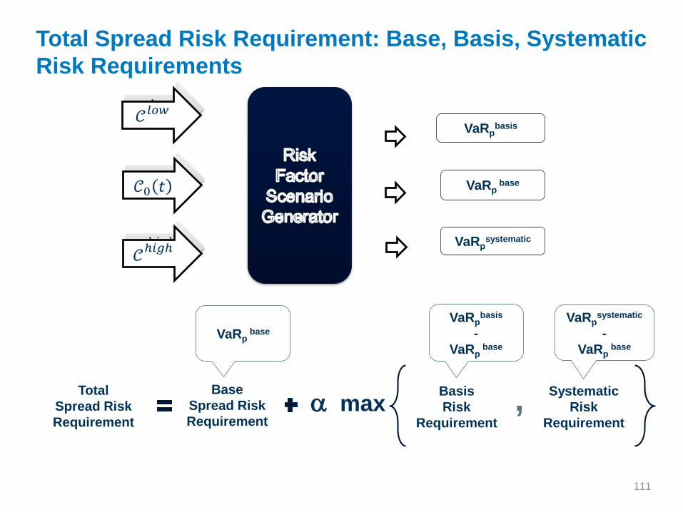
Total Spread Risk Requirement: Base, Basis, Systematic

Risk Requirements

VaRpbase

VaRpbasis

VaRpsystematic

VaRpsystematic

-

VaRpbase

VaRpbasis

-

VaRpbase

Total

Spread Risk

Requirement

Basis

Risk

Requirement

Base

Spread Risk

Requirement

Systematic

Risk

Requirement

,a max

𝒞0 𝑡

𝒞ℎ𝑖𝑔ℎ

𝒞𝑙𝑜𝑤

VaRpbase

𝒞0 𝑡

𝒞ℎ𝑖𝑔ℎ

𝒞𝑙𝑜𝑤

112

Impact of High, Low, Base Correlation Matrix on Spread

Risk Requirement : Basis Exposure

-$100,000

-$50,000

$0

$50,000

$100,000

$150,000

$200,000

$250,000

$300,000

1/2

0/2

01

0

4/2

0/2

010

7/2

0/2

01

0

10/2

0/2

010

1/2

0/2

01

1

4/2

0/2

01

1

7/2

0/2

01

1

10/2

0/2

011

1/2

0/2

01

2

4/2

0/2

01

2

7/2

0/2

01

2

10/2

0/2

012

1/2

0/2

01

3

4/2

0/2

01

3

7/2

0/2

01

3

10/2

0/2

013

Butterfly : Long 1 Year / Short 3 Year / Long 10 Year Protection on Levi Strauss & Company (SDV01 Neutral)

5-Day Loss Systematic VaR Base VaR Basis VaR Spread Risk Requirement

113

Jump-to-Default (JTD) and Jump-to-Health Risk Requirements

JTD and JTH risk requirements are add-on risk charges to cover for the

default and drastic improvement in credit quality of one entity

Credit entities are removed one at a time from the portfolio

Base spread requirement of the remaining portfolio is re-calculated

For JTD, index position scenario P&L’s are reduced by a ratio of 1 / #(index constituents)

For JTH, index position scenario P&L’s are not adjusted

Each spread scenario P&L is added a JTD and JTH P&L for the removed entity

For JTD: (Total Single Name Notional with Index Decomposition) x (RR – Current Price)

For JTH: (Single Name Notional) x (Price @ Low Percentile (%0.5) Spread of High Correlation

Scenarios – Current Price)

JTD and JTH quantiles are calculated from the new scenario P&L’s: for each

entity k, VaRpidio,k

The final JTD and JTH risk requirements are calculated as maxk{ VaRpJTD,k }

– VaRp and maxk{ VaRpJTH,k } – VaRp, respectively

114

Interest Rate Sensitivity Charge

This charge covers losses due to changes in interest rate term

structure,

The sensitivity is mainly to the parallel upward and downward shifts of

the interest rate (IR) curve

Log-return history of

the 5 Year Rate from

the IR curve

Up shock

99% quantile

Down shock

1% quantile

Scenario Up

IR curve

Scenario Down

IR curve

P&L up

P&L down

IRS charge = - min {P&L down, P&L up}

115

Stress Extension for GF calculations

The stress model is an extension of the margin model

The stress spread risk requirement is calculated from a higher percentile of

the P&L distribution across scenarios: VaRq where q = %99.75

The number of obligors considered for JTD is two instead of 1

The JTH spread is computed from a lower (0.05%) percentile of the high

correlation scenarios

The spread risk requirement is the maximum of base, basis and systematic

stress VaR : 𝛼𝑆𝑡𝑟𝑒𝑠𝑠 = 1

The interest rate risk requirement is computed from %0.25 and %99.75

percentile of historical log changes of the 5 year point on the IR curve

116

Model Parameters and Calibration : Summary for Margin

and Stress Calculations MARGIN STRESS

Parameter Calibration Value Calibration Value

JTH QuantileHigh Correlation

Scenarios0.50%

High Correlation

Scenarios0.05%

VaR Quantile 10,000 Scenarios 99.00% 10,000 Scenarios 99.75%

Copula Student-t DoF 3 3

Risk Factor Student-t DoF [ t 0,i , t M ] [ t 0.i , t M ]

EWMA Scaling Parameter 0.97 0.97

EWMA Volatility [ t - 252 , t-1 ] [ t - 252 , t-1 ]

EWMA Volatility Forecast [ t M -252 , t M ] [ t 0,i , t M ]

Countercyclical Volatility [ t 0,i , t M ] [ t 0,i , t M ]

Historical Correlation Matrix [ t M - 504 , t M ] [ t M - 504 , t M ]

Low Correlation Matrix 0 (Ind/Ind : 0.5) 0 (Ind/Ind : 0.5)

High Correlation Matrix 1 1

Autocorrelation [ t M - 504 , t M ] [ t M - 504 , t M ]

Countercyclical Autocorrelation [ t 0,i , t M ] [ t 0,i , t M ]

Number of JTD/JTH Entities 1 / 1 2 / 1

Minimum Recovery Rate (JTD) [ t 0,i , t M ] [ t 0,i , t M ]

Correlation Charge Factor 0.25 1

Interest Rate Quantile [ t 0,i - 1260 , t M ] 1% / 99% [ t 0,i - 1260 , t M ] 0.25% / 99.75%

t M : Margin/Stress date t 0,i : Earliest date which has market data for risk factor i

I Item

117

Backtesting Portfolios and Strategies

Targeted Portfolios

StrategyExamples

(Buy, Sell) (Sell, Buy) (Buy, Sell)

Curve

IG 5 IG 10

HY 5 HY 10

SN 5 SN 10

IG 1 IG 5 IG 10

Pair

IG 5 HY 5

SN 5 HY 5

IG 5 SN 5

SN i 5 SN j 5

RollIG OTR 5 IG OTR-n 5

HY OTR 5 HY OTR-n 5

Pair x Curve IG 5 HY 10

Directional DV01 Zero SDV01 Zero

Diversified Portfolios

StrategyExamples

(Buy, Sell) (Sell, Buy) (Buy, Sell)

Index Arbitrage IG 5IG Constituents

5

BasisIG 5 Financials 5

High Spread 5 Low Spread 5

CurveFinancials 5 Financials 10

Technology 1 Technology 5 Technology 10

Sector Industrials 5Consumer

Goods 5

Basis x Curve IG 10IG Constituents

5

Sector x Curve Financials 5Consumer

Services 10

118

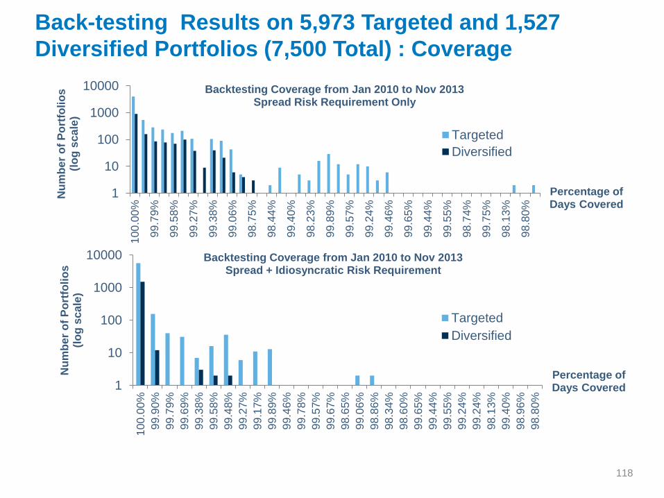
Back-testing Results on 5,973 Targeted and 1,527

Diversified Portfolios (7,500 Total) : Coverage

1

10

100

1000

10000

100

.00

%

99.7

9%

99.5

8%

99.2

7%

99.3

8%

99.0

6%

98.7

5%

98.4

4%

99.4

0%

98.2

3%

99.8

9%

99.5

7%

99.2

4%

99.4

6%

99.6

5%

99.4

4%

99.5

5%

98.7

4%

99.7

5%

98.1

3%

98.8

0%

Nu

mb

er

of

Po

rtfo

lio

s

(lo

g s

ca

le)

Percentage of Days Covered

Backtesting Coverage from Jan 2010 to Nov 2013Spread Risk Requirement Only

Targeted

Diversified

1

10

100

1000

10000

100

.00

%

99.9

0%

99.7

9%

99.6

9%

99.3

8%

99.5

8%

99.4

8%

99.2

7%

99.1

7%

99.8

9%

99.4

6%

99.7

8%

99.5

7%

99.6

7%

98.6

5%

99.0

6%

98.8

6%

98.3

4%

98.6

0%

99.6

5%

99.4

4%

99.5

5%

99.2

4%

99.2

4%

98.1

3%

99.4

0%

98.9

6%

98.8

0%

Nu

mb

er

of

Po

rtfo

lio

s

(lo

g s

ca

le)

Percentage of Days Covered

Backtesting Coverage from Jan 2010 to Nov 2013Spread + Idiosyncratic Risk Requirement

Targeted

Diversified

119

Backtesting Results on 7500 Portfolios : Sample

Diversified Portfolios

-$800,000

-$600,000

-$400,000

-$200,000

$0

$200,000

$400,000

$600,000

$800,000

1/2

0/2

01

0

4/2

0/2

01

0

7/2

0/2

01

0

10/2

0/2

01

0

1/2

0/2

01

1

4/2

0/2

01

1

7/2

0/2

01

1

10/2

0/2

01

1

1/2

0/2

01

2

4/2

0/2

01

2

7/2

0/2

01

2

10/2

0/2

01

2

1/2

0/2

01

3

4/2

0/2

01

3

7/2

0/2

01

3

10/2

0/2

01

3

Basket of Financials: Long 10 Year / Short 5 Year Protection (DV01 Neutral)

5-Day Loss Sprad Risk Requirement Spread Risk Requirement (Flip)

-$30,000

-$20,000

-$10,000

$0

$10,000

$20,000

$30,000

1/2

0/2

01

0

4/2

0/2

01

0

7/2

0/2

01

0

10/2

0/2

01

0

1/2

0/2

01

1

4/2

0/2

01

1

7/2

0/2

01

1

10/2

0/2

01

1

1/2

0/2

01

2

4/2

0/2

01

2

7/2

0/2

01

2

10/2

0/2

01

2

1/2

0/2

01

3

4/2

0/2

01

3

7/2

0/2

01

3

10/2

0/2

01

3

Index Arbitrage: Short 5 Year Index / Long 5 Year Constituent Protection (SDV01 Neutral)

5-Day Loss Sprad Risk Requirement Spread Risk Requirement (Flip)

Portfolio

Spread Risk

/ Gross

Notional

Coverage

Original 1.5% 100%

Flip 1.3% 99.90%

Portfolio

Spread Risk

/ Gross

Notional

Coverage

Original 0.6% 100%

Flip 0.6% 99.90%

120

Number of Monte Carlo Scenarios : Production Margin

Sensitivity Across CMF’s

$0

$100,000,000

$200,000,000

$300,000,000

$400,000,000

$500,000,000

$600,000,000

$700,000,000

$800,000,000

5,000 10,000 20,000 30,000 40,000 50,000

13 12 11 10 9 8 7 6 5 4 3 2 1

121

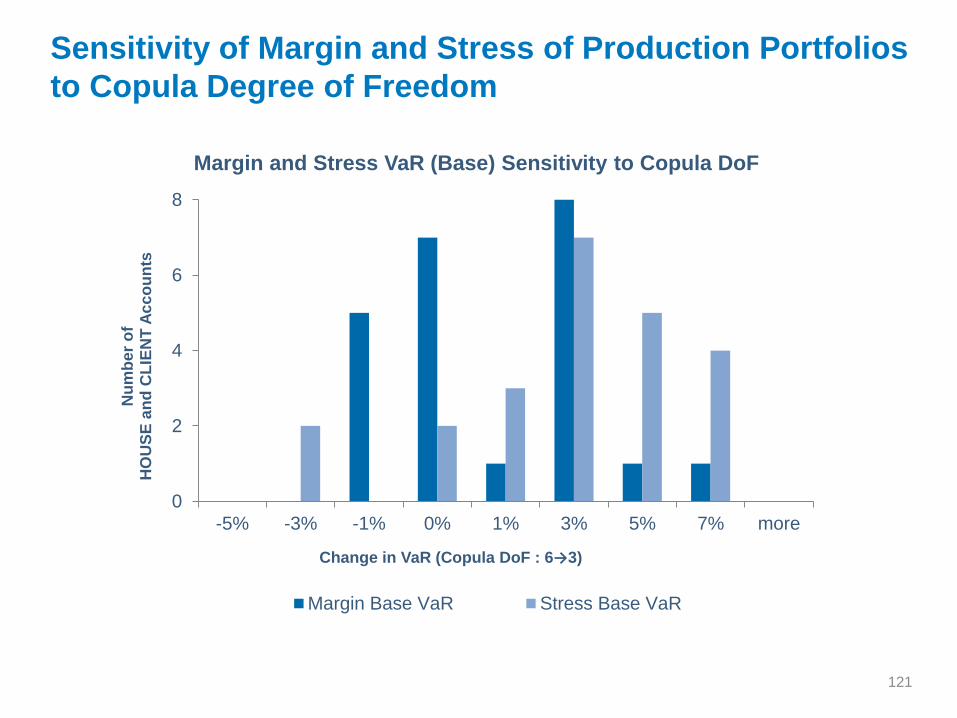
Sensitivity of Margin and Stress of Production Portfolios

to Copula Degree of Freedom

0

2

4

6

8

-5% -3% -1% 0% 1% 3% 5% 7% more

Nu

mb

er

of

HO

US

E a

nd

CL

IEN

T A

cc

ou

nts

Change in VaR (Copula DoF : 6→3)

Margin and Stress VaR (Base) Sensitivity to Copula DoF

Margin Base VaR Stress Base VaR

CME CDS Clearing

Jump to Default and Jump to

Health Requirements

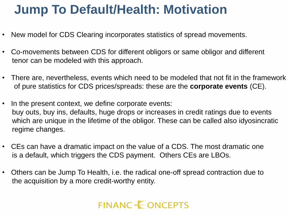
Jump To Default/Health: Motivation

• New model for CDS Clearing incorporates statistics of spread movements.

• Co-movements between CDS for different obligors or same obligor and different

tenor can be modeled with this approach.

• There are, nevertheless, events which need to be modeled that not fit in the framework

of pure statistics for CDS prices/spreads: these are the corporate events (CE).

• In the present context, we define corporate events:

buy outs, buy ins, defaults, huge drops or increases in credit ratings due to events

which are unique in the lifetime of the obligor. These can be called also idyosincratic

regime changes.

• CEs can have a dramatic impact on the value of a CDS. The most dramatic one

is a default, which triggers the CDS payment. Others CEs are LBOs.

• Others can be Jump To Health, i.e. the radical one-off spread contraction due to

the acquisition by a more credit-worthy entity.

Definition of JTH/JTD in the Model

• CE’s are rare events for a single company, but they may be frequent in

a large multi-obligor portfolio

• We wish to detect vulnerabilities in a portfolio to corporate events. We

assume that on the period of interest, only one obligor experiences such

CE.

• A JTD event in a portfolio means that one obligor defaults,

triggering the CDS protection and the portfolio is short protection in that

name

• AT JTH event means that the spreads of a particular obligor contract dramatically

to tail risk levels of 99.75%. (This is a parametric assumption, which will need

to be validated.

Computation of JTD charge

• Step 1: Tally all the obligors for which the portfolio is short protection.

Assume that there are 𝑁𝑠 such names. Let 𝜋1, 𝜋2,…, 𝜋𝑁𝑠 denote

the sub-portfolios that exclude each of the names (complementary

portfolios.

• Step 2: For each name for which the portfolio is short protection, compute

the loss given default:

𝐿𝐺𝐷𝑖 =

𝑘

𝑛𝑖𝑘 𝑃𝑖𝑘 − 𝑅𝑅𝑖

Here 𝑛𝑖𝑘 (negative) is the notional amount and 𝑃𝑖𝑘is the value of the

CDS. The sum is made over tenors.

• Step 3: Compute the market risk charge for each complementary

portfolio, e. g. , 𝑀𝑅 𝜋𝑖 = 𝐸𝑆.99 𝜋𝑖 , 5𝑑𝑎𝑦 ℎ𝑜𝑟𝑖𝑧𝑜𝑛

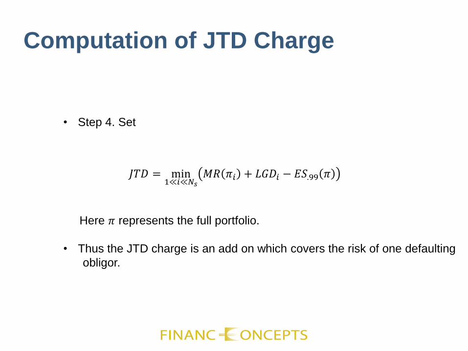
Computation of JTD Charge

• Step 4. Set

Here 𝜋 represents the full portfolio.

• Thus the JTD charge is an add on which covers the risk of one defaulting

obligor.

𝐽𝑇𝐷 = min1≪𝑖≪𝑁𝑠

𝑀𝑅 𝜋𝑖 + 𝐿𝐺𝐷𝑖 − 𝐸𝑆.99 𝜋

Computation of JTH Charge

• Step 4. Define the JTH charge as

𝐽𝑇𝐻 = min1≤𝑖≤𝑁𝑙

𝑀𝑅 𝜋𝑖 + 𝐿𝐺𝐻𝑖 − 𝐸𝑆.99 𝜋

Total Charge for JTH/JTD

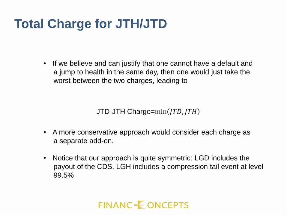
• If we believe and can justify that one cannot have a default and

a jump to health in the same day, then one would just take the

worst between the two charges, leading to

• A more conservative approach would consider each charge as

a separate add-on.

• Notice that our approach is quite symmetric: LGD includes the

payout of the CDS, LGH includes a compression tail event at level

99.5%

JTD-JTH Charge=min 𝐽𝑇𝐷, 𝐽𝑇𝐻

Epilogue:

What is the incoming U.S. Administration’s

proposal for financial regulation?

129

130From Rep. Jeb Hensarling’s office.

Now considered for Secretary of Treasury

131

132

133

134

135

136

137

138

139

140

141

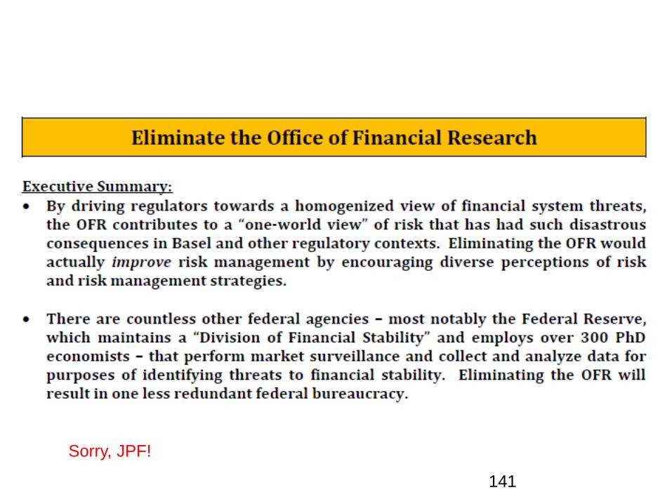
Sorry, JPF!

142

143

144

145

146