LSE Research Online Article (refereed)
Eric Neumayer
Does the “resource curse” hold for growth in genuine income as well?
Originally published in World development, 32 (10). pp. 1627-1640 © 2004 Elsevier Ltd. You may cite this version as: Neumayer, Eric (2004). Does the “resource curse” hold for growth in genuine income as well? [online] London: LSE Research Online. Available at: http://eprints.lse.ac.uk/archive/00000626 Available online: February 2006 LSE has developed LSE Research Online so that users may access research output of the School. Copyright © and Moral Rights for the papers on this site are retained by the individual authors and/or other copyright owners. Users may download and/or print one copy of any article(s) in LSE Research Online to facilitate their private study or for non-commercial research. You may not engage in further distribution of the material or use it for any profit-making activities or any commercial gain. You may freely distribute the URL (http://eprints.lse.ac.uk) of the LSE Research Online website. This document is the author’s final manuscript version of the journal article, incorporating any revisions agreed during the peer review process. Some differences between this version and the publisher’s version remain. You are advised to consult the publisher’s version if you wish to cite from it.
http://eprints.lse.ac.uk Contact LSE Research Online at: [email protected]
Does the ‘Resource Curse’ hold for Growth in
Genuine Income as well?
Eric Neumayer∗
London School of Economics
FINAL VERSION
∗ Department of Geography and Environment and Center for Environmental Policy and
Governance (CEPG), London School of Economics and Political Science, Houghton Street,
London WC2A 2AE, UK
Phone: +44-207-955-7598. Fax: +44-207-955-7412. Email: [email protected]
Summary. –– Existing studies analyzing the so-called ‘resource curse’ hypothesis
regress growth in gross domestic product (GDP) on some measure of resource-intensity.
This is problematic as GDP counts natural and other capital depreciation as income.
Deducting depreciation from GDP to arrive at genuine income, we test whether the
‘curse’ still holds true. We find supporting evidence, but the growth disadvantage of
resource-intensive economies is slightly weaker in terms of genuine income than GDP.
We suggest that this provides additional, but somewhat weak and limited, evidence in
support of those who argue that the ‘curse’ is partly due to unsustainable over-
consumption.
Key words –– global; resource curse hypothesis; natural capital; depreciation; genuine
income; genuine savings
1
ACKNOWLEDGEMENT
I would like to thank three anonymous reviewers for many helpful and constructive
comments. All remaining errors are mine.
2
1. INTRODUCTION
Being richly endowed with natural resources can threaten a country’s long-term
prosperity as natural resource-intensive economies grow slower over time than
economies that are less natural resource-intensive. Sachs and Warner (1995a) were not
the first one to note this paradoxical result,1 but their paper spurred an extensive and still
growing literature aimed at explaining what drives this result (e.g., Mikesell, 1997; Auty
and Mikesell, 1998; Ross, 1999; Auty, 2001; Manzano and Rigobon 2001; Isham et al.,
2003; Sala-i-Martin and Subramanian, 2003).2 These studies offer a diverse set of
explanations covering, amongst others, terms of trade effect, dutch disease, debt
overhang, institutional quality and other political economy arguments. Others
questioned the robustness of the result with respect to changes in the definition of
natural resource-intensity (e.g., Stijns, 2001a) and the econometric estimator used (e.g.,
Manzano and Rigobon, 2001) or observed that in terms of income levels (rather than
growth) natural resource-intensive economies on average fare better rather than worse
(e.g., Davis, 1995; Mikesell, 1997; Gallup, Sachs and Mellinger, 1999).
In this article, we do not seek to explain the so-called ‘resource curse’ directly.
Neither do we seek to test whether the ‘curse’ still holds for competing definitions of
resource intensity or alternative estimation techniques. Instead, this paper’s original
contribution is in examining whether the ‘curse’, as postulated by Sachs and Warner
(1995a, 1997), holds true for measures of genuine or true income as well. This is
important because GDP is a particularly erroneous measure of income for resource-
intensive economies.
Existing studies look at growth in real gross domestic product (GDP). Of course, it
is well known that GDP contains an element of depreciation of produced capital that
should not be counted as income. It would therefore be more correct to analyze growth
3
in real net domestic product (NDP) where depreciation of produced capital has been
subtracted from GDP. This is typically not done for two reasons. First, the depreciation
term is estimated based on simplifying (and contestable) assumptions and, more
importantly, for most countries it makes very little difference whether one looks at GDP
or NDP. This holds true whether or not economies are intensive in natural resources.
Things are different, however, when one starts taking into account depreciation of
natural capital as well. Not only can depreciation terms be of significant size, but also
depreciation tends to be higher for economies that are intensive in natural resources than
for others that are not. With the accounting method for natural capital depreciation
described below the correction to GDP can be as high as 30 per cent. There can
therefore be a substantial gap between gross income and what one might want to call
genuine income, that is GDP minus the depreciation of produced and natural capital,
and the size of the gap is partly determined by the resource-intensity of economies.
There is therefore a problem with the existing studies examining the ‘resource curse’ as
they analyze growth in GDP instead of growth in true or genuine income.
This article therefore tests whether the ‘resource curse’ holds true for growth in
genuine income as well and, if so, whether the negative effect of natural resource-
intensity on growth is over- or under-estimated by erroneously examining growth in
GDP. To our knowledge, no other study has ever done this. Winter-Nelson (1995)
computes what he calls environmentally adjusted income for 18 African resource
exporters, but he merely demonstrates that a strategy of export expansion has led to
growth in GDP, but not growth in environmentally adjusted income. He therefore does
not test for the ‘resource curse’ itself. Also, his sample size is of course very small.
Mikesell (1997, p. 195) suggests that if GDP was adjusted for natural capital
depreciation, then the ‘resource curse’ would be even stronger over the period 1980 to
4
1993. However, he does not validate his suggestion with any general empirical test,
instead referring to Repetto et al.’s (1989) single country study of Indonesia, in which
adjusted income grew slower over the period 1971 to 1984 than GDP. Indeed, we will
show that the exact opposite to Mikesell’s suggestion is actually the case as the
‘resource curse’ is slightly weaker in terms of growth of genuine income than growth of
GDP.3 Atkinson and Hamilton (2003) examine whether negative genuine savings rates
(gross investment minus depreciation of produced and natural capital divided by GDP)
can explain the ‘resource curse’, but they do not examine whether the ‘curse’ holds for
growth in genuine income.
2. EXPLAINING THE ‘RESOURCE CURSE’
How can the blessing of an extra endowment with natural resources turn into a curse? A
priori this represents a puzzle, even a paradox. Following Auty (2001) one can
distinguish ‘exogenous’ from ‘internal’ explanations for the poor growth performance
of natural resource-intensive economies. Revenue volatility and a long-term declining
trend in the terms of trade of resource exporters represent explanation attempts that can
be derived from structuralist economic theory à la Prebisch (1950). The Dutch disease
phenomenon is another and one of the most frequently cited exogenous explanations. It
refers to the decline in the productivity and competitiveness of the manufacturing and
other tradeables sector following the real exchange rate appreciation in the wake of a
resource boom. This represents a problem if the manufacturing and other tradeables
sector is characterized by economies of scale (Gelb and associates, 1988; Sachs and
Warner, 2001). The exogenous explanations leave little space for policy makers to avoid
the problem. In comparison, the internal explanations of the ‘resource curse’ all lay the
blame squarely at bad policies. A link between the two is given by the fact that the
5
manufacturing and other tradeables sector becomes damaged not only by dutch disease,
but also by misguided industrial policies in the form of protectionist barriers for import-
substitution, which has been typical for many natural resource-intensive economies.
Indeed, some studies show that the main problem of resource booms was to allow
resource-intensive economies to sustain economically harmful policies longer than less
resource-intensive economies that started out with similarly unproductive policies (e.g.,
Auty 1993, 1994). More importantly, resource abundance might lead to a rentier
economy with a predatory state: corruption, political conflict and inequalities are
rampant, economic institutions are poorly developed, human capital accumulation,
entrepeneurship and innovative activity are crowded out and policy makers are more
interested in resource transfers than developing and modernizing the country’s economy
(Lal and Myint, 1996; Gylfason, 2001; Auty, 2001; Isham et al., 2003).4
Two studies have emphasized the problem that natural resource abundance allows
countries to engage in excessive consumption that is not sustainable into the future. We
will concentrate on these two studies as our empirical analysis provides some, but
limited, evidence in their favor. Rodríguez and Sachs (1999) employ a Ramsey growth
model and a calibrated dynamic general equilibrium model of the Venezuelan economy
to argue that economies rich in natural resources are likely to live beyond their means.
Indicative of this is that resource-intensive economies, whilst growing slower than less
resource-intensive ones, also tend to have higher absolute income levels – a point
demonstrated by Rodríguez and Sachs (1999), but already pointed out by others (e.g.,
Davis, 1995; Mikesell, 1997). In the transition to the steady state, the resource
endowment allows the country to afford extraordinary consumption possibilities derived
from unsustainably high income levels. In other words, ‘a resource rich economy will
adjust to its steady state from above, not from below’ (Rodríguez and Sachs, 2003, p. 4).
6
During the transition it might display negative growth rates in GDP on average. With
exogenous productivity growth it might escape negative growth rates, but in any case
growth rates will be lower than if the country did not live on unsustainable income
levels beyond its means. Theoretically, the problem could be circumvented if the
resource-intensive economy invests its resource rents in international assets paying
permanent annuities. However, if there are restrictions on investment abroad or a
preference for investing domestically, then these economies will experience
consumption booms that are unsustainable in the long run. Of course, on a very
fundamental level it is not clear that such consumption booms are completely irrational
and undesirable. Even a rational inter-temporal social welfare maximizer might want to
use some of the windfall gains from resource booms to raise initial consumption levels.
This is because the marginal utility of consumption in these economies is likely to be
very high and if exogenous productivity growth can be expected then the windfalls can
also be used to smooth the inter-temporal consumption path.
Atkinson and Hamilton (2003) provide an argument similar to Rodríguez and Sachs
(1999) together with corroborating evidence from cross-sectional growth in GDP
regressions. They argue that resource-intensive countries, defined as countries with a
high share of natural capital depreciation relative to GDP, are likely to have excessive
consumption fuelled by the windfalls of natural resource extraction. Their regressions
show that the interaction of large resource rents with government consumption is
associated with lower growth. Atkinson and Hamilton (2003) also find that natural
resource-intensity in economies with negative genuine savings rates is associated with a
growth rate that is statistically significantly below zero. Natural resource-intensity in
economies with a positive genuine savings rate is also estimated to have a negative
coefficient, but it is not statistically significant.5 Furthermore, whilst Sachs and Warner
7
(1997) did not find evidence that resource-intensity is associated with lower gross
savings and investment rates, Atkinson and Hamilton (2003) on the whole find a
negative correlation between natural resource-intensity and genuine savings rates.
Gylfason and Zoega (2002) find a similar link between investment and savings rates on
one hand and resource abundance on the other hand, where resource abundance is
defined as the share of natural capital in total national wealth.
Let us turn to a discussion on how one should account for natural capital
depreciation and the implications of such accounting for the ‘resource curse’.
3. ACCOUNTING FOR NATURAL CAPITAL DEPRECIATION
Resource economists have studied the importance of as well as methods for accounting
for natural capital depreciation at least since Hartwick’s (1977) influential paper. There
he showed that under certain circumstances economies, which extract a non-renewable
resource, can only maintain their consumption levels over time if they invest the full
resource rents into produced capital. Throughout the 1980s and the 1990s accounting for
natural capital depreciation has figured prominently in natural resource economics as
part of the sustainable development research agenda (El Serafy, 1981, 1989; Repetto et
al., 1989; Serôa da Motta and Young, 1995).
That the GDP of natural resource-intensive economies does not reflect their genuine
income levels has not escaped the early attention of affected countries either. For
example, Shihata (1982, p. 202), then Director-General of the Organisation of
Petroleum Exporting Countries (OPEC) Development Fund, notes that the income of
the Arab oil-exporting economies ‘is in reality a cash exchange for a depletable natural
resource’. OPEC itself commissioned a study in 1984, which opens with a sentence of
admirable clarity: ‘The GDP of oil-exporting states is exaggerated because some of their
8
“income” is due to the consumption of depletable oil resources and hence is liquidation
of capital, not income’ (Stauffer and Lennox, 1984, p. 6).
Unfortunately, how best to account for natural capital depreciation is heavily
debated and no consensus has emerged in the relevant literature (Hartwick and
Hageman, 1993; El Serafy, 1981, 1989; Vincent, 1997; Santopietro, 1998). It does have
a very simple answer, however, as long as one assumes that economies are competitive
and inter-temporally efficient (Hartwick and Hageman, 1993; Hamilton, 1996;
Neumayer, 2003). In this framework natural capital depreciation is equal to total
Hotelling (1931) rent:
(1) RMCP ⋅− )(
where P is the resource price, MC is marginal cost and R is resource extraction. In
the case of a renewable resource, R would be resource harvesting beyond natural
regeneration. One of the major difficulties of applying this theoretically correct method
in reality is that data on marginal cost are frequently unavailable. Average cost data are
more available. Most studies applying this method have therefore replaced marginal
cost with the more readily available average costs and calculated depreciation according
to the following formula:
(2) ( )P AC R− ⋅
A popular alternative has been what is known as the El Serafy (1981, 1989) method:
9
(3) ( )( )
P AC Rr n
− ⋅ ⋅+
⎡
⎣⎢
⎤
⎦⎥+
11 1
where r is the discount rate and n is the number of remaining years of the resource
stock. For simplicity, n is often set equal to the static reserves to production ratio, which
is the number of years the reserve stock would last if production was the same in the
future as in the base year. If r > 0 and n > 0, then (3) will produce a smaller depreciation
term for resource extraction than (2).
Equation (3) is also called the ‘user cost’ of resource extraction since it indicates the
share of resource receipts that should be considered as capital depreciation. The formula
for the El Serafy method is derived from the following reasoning: receipts from non-
renewable resource extraction should not fully count as what El Serafy calls ‘sustainable
income’ because resource extraction leads to a lowering of the resource stock and thus
brings with it an element of depreciation of the resource capital stock.6 Whilst the
receipts from the resource stock will end at some finite time, ‘sustainable income’ by
definition must last forever. Hence, ‘sustainable income’ is defined as that part of
resource receipts which if received infinitely would have a present value just equal to
the present value of the finite stream of resource receipts over the life-time of the
resource. Natural capital depreciation is then the difference between resource rents and
‘sustainable income’. Appendix 1 shows why this reasoning leads to equation (3).
Hartwick and Hageman (1993) show that the El Serafy method can be understood
as an approximation to equation (1), which to repeat represents the theoretically correct
depreciation in a framework of a competitive inter-temporally efficient economy. Its
main advantage over the World Bank method in equation (2) is that the El Serafy
method can use average cost without apology as it does not depend on marginal cost.
The World Bank method, on the other hand, needs to replace marginal cost with average
10
cost as marginal cost is not readily available. Due to the replacement of marginal with
average cost it can also merely represent an approximation to the theoretically correct
method. Which of the two methods creates the greater bias is therefore not clear in
general. Under certain assumptions about the resource extraction cost function, the two
methods can be shown to be two polar cases of the true depreciation value and the bias
depends on the elasticity of the marginal cost curve with respect to the quantity
extracted (Vincent, 1997; Serôa da Motta and Ferraz do Amaral, 2000).
In this study, we will use the method given by (2). The main reason is that reliable
reserve data of natural resources are difficult to get hold of.7 Additionally, as long as
known reserves last for less than or little more than 20 years or so, which typically holds
true for many resource-intensive economies, and the discount rate is significantly below
5 per cent, then the difference between (2) and (3) is not that large (Atkinson and
Hamilton, 2003). To show this, table 1 plots for various values of n and r the difference
between (2) and (3) for a natural capital depreciation value of $100 according to (2). A
low discount rate can be justified on the grounds that it is highly uncertain whether the
alternative investments that are supposed to provide an infinite stream of income can be
expected to generate a high rate of return. An additional justification for using (2) is that
unexpected developments such as breakthroughs in the price of substitute backstop
technologies can hugely decrease the value of large reserve stocks and the longer the
stock lasts in the future the more uncertainty there is.
< Insert Table 1 about here >
11
4. ACCOUNTING FOR NATURAL CAPITAL DEPRECIATION
AND THE ‘RESOURCE CURSE’
With (2) as the formula for computing natural capital depreciation, how is the growth
performance in genuine income levels likely to differ from the growth performance in
GDP? Ceteris paribus, the ‘resource curse’ is stronger (weaker) in terms of growth of
genuine income than growth in GDP if the start period depreciation term relative to
GDP is smaller (bigger) than the end period depreciation term relative to GDP. This of
course depends on the depreciation term in the start period compared to the end period
of analysis, but it also depends on their sizes relative to the respective GDP levels from
the two periods. Recall that the depreciation term is (P-AC)·R. Average extraction levels
tend to have risen between 1970 and 1998. For extraction costs, the trend is very much
resource- and country-specific. Prices of resources have also not trended uniformly over
this period as table 2 shows.8
< Insert Table 2 about here >
Some prices like that of oil, the most important component of natural capital
depreciation in value terms, and gold have gone up, whereas the price of many others
have fallen. This already implies that a priori it is not clear whether accounting for
natural capital depreciation weakens or strengthens the ‘resource curse’. However,
because what matters is the size of (P-AC)·R relative to GDP levels, the impact of
accounting for natural capital depreciation on the ‘resource curse’ gets even more
complex. One therefore needs to employ theory to arrive at a more informed prior
expectation about the strength of the ‘resource curse’ in terms of growth of genuine
income compared to GDP growth. It is here that Rodríguez and Sachs’s (1999) and
12
Atkinson and Hamilton’s (2003) arguments are informative. If it is true that resource-
intensive economies have excessive consumption spurred by unsustainably high GDP
levels, then the growth performance in genuine income levels should be better than the
growth performance in GDP, which is boosted by unsustainable resource extraction.
This is because genuine income levels are corrected for depreciation of natural capital.
They take out the unsustainable parts of GDP. It follows that one can expect the
‘resource curse’, if it exists at all, to be weaker in terms of growth of genuine income
than growth of GDP. It is this hypothesis we are going to test now.
5. RESEARCH DESIGN
To demonstrate clearly the effect of natural resource-intensity on growth in genuine
income rather than growth in GDP we use Sachs and Warner’s (1997) original data set
with amendments. We briefly describe the variables used here, but appendix 2 also
provides detailed and more precise variable definitions and states the sources of data.
Maloney (2001, p. 1) criticizes Sachs and Warner’s (1997) results on the ground that
‘growth processes take place across the very long run and probably cannot be
convincingly summarized by cross section regressions of one highly turbulent 20 year
period at the end of the 20th century’. Unfortunately, no data on natural capital
depreciation exist before 1970 so that we cannot extend the period of analysis
backwards. However, since we have now access to more updated data, we no longer
restrict the analysis to the period 1970 to 1990, but extend it to 1998 making use of the
latest update of the Penn World Tables (Heston, Summers and Aten 2002).
Like Sachs and Warner (1997) we start with regressing the average annual growth
rate in GDP over the period 1970 to 1998 (GROWTH7098) on the log of initial GDP per
capita (LGDP70) and the variable of natural resource-intensity. For our measure of
13
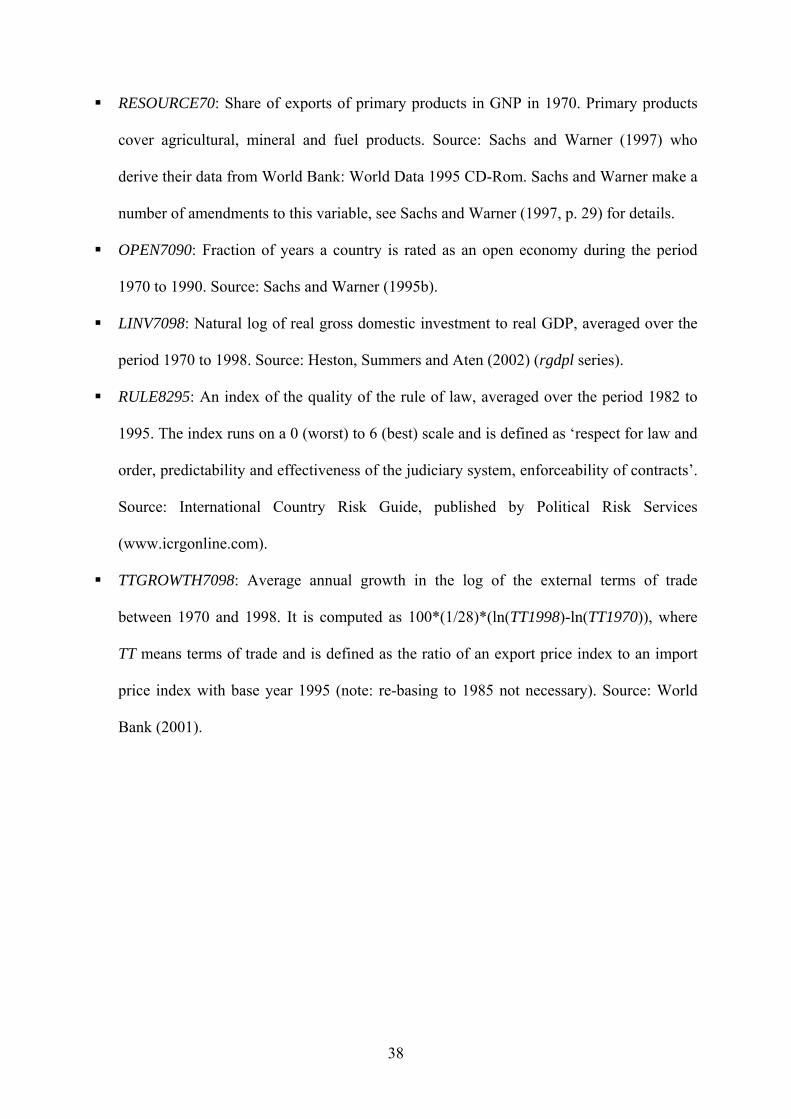
natural resource-intensity we follow Sachs and Warner and use their measure of the
share of exports of primary products in GNP in 1970 (RESOURCE70).9 Primary
products consist of agricultural products, minerals and energy resources. Following the
structure of Sachs and Warner’s (1997) basic regressions, we then add their measure of
trade openness (OPEN7090). Unfortunately, this variable could not be updated to 1998.
In consequent regressions follow the log of the average gross investment to GDP ratio
(LINV7098), a measure capturing the average extent of the rule of law (RULELAW8295)
and the average annual growth in the log of the external terms of trade between 1970
and 1998 (TTGROWTH7098). The rule of law variable is not publicly available, but has
been provided for the better part of the period of this study free of charge courtesy of
Political Risk Services. Note that this variable does not exist before 1982 so that the
extent of the rule of law is averaged over the period 1982 to 1995. We then repeat the
set of regressions with growth in genuine income as the dependent variable
(GENGROWTH7098) and replace LGDP70 with the log of the initial genuine income
level (LGENINC70).10
Like Sachs and Warner (1997) we exclude outliers from the sample applying
Belsley et al.’s (1980) criterion. An outlier is an observation with a DFITS that is
greater in absolute terms than twice the square root of (k/n), where k is the number of
independent variables and n the number of observations, and where DFITS is defined as
the square root of (hi/(1-hi)), where hi is an observation’s leverage, multiplied by its
studentized residual. Applying this criterion excludes Botswana, Gabon, Malaysia,
Rwanda and Zambia from the sample. However, like in Sachs and Warner (1997) the
main results uphold if these countries are not excluded.
We take the values of produced and natural capital depreciation from the World
Bank’s data set on genuine savings, also called adjusted net savings, published on the
14
Bank’s website and available as part of the annual World Development Indicators on
CD-Rom.11 Clearly, depreciation of both produced and natural capital should be taken
into account, but non-reported sensitivity analysis showed that natural capital
depreciation is the main driver of the results reported below.
The World Bank takes data on the depreciation of produced capital from estimates
undertaken by the United Nations Statistics Division. With respect to natural capital
depreciation, the World Bank data set includes three categories of natural resources,
namely energy, minerals and forestry. Energy consists of oil, gas and coal, whereas
minerals encompass bauxite, copper, iron ore, lead, nickel, phosphate rock, tin, zinc,
gold and silver. Forestry refers to the production of fuelwood, coniferous softwood,
non-coniferous softwood and tropical hardwood.12 For minerals, (P-AC), or unit rent, is
computed as the world price of the resource minus mining, milling, benefication,
smelting and transportation to port costs minus a ‘normal’ return to capital. For oil, gas
and coal, unit rent is the world price minus lifting costs. For some resources, such as
natural gas, where, strictly speaking, there is no single world price, a shadow world
price is computed as the average free-on-board price from several points of export. For
forestry, unit rent is calculated as the world price for each category of wood minus
average unit production costs. This is multiplied by the amount of wood production
exceeding the natural increment.
Inevitably, there are some problems with the data. For example, the use of uniform
world prices overstates somewhat natural capital depreciation for countries with lower-
grade resource deposits. The use of average rather than marginal costs also tends to
over-estimate depreciation. Both prices and extraction costs often need to be estimated.
Extraction costs are sometimes only available for a region rather than countries and only
for a number of years, which means that missing values need to be interpolated.
15
Furthermore, for lack of data the World Bank’s computations of natural capital
depreciation do not cover such items as depletion of fish stocks and water resources and
the erosion of topsoil. This together with natural capital depletion being computed by
the net price instead of the user cost method (see section 3 above) implies that the
natural capital depreciation of mineral and fossil fuel extracting economies is somewhat
biased upwards relative to that of other economies.13 These caveats notwithstanding, the
data set represents the most ambitious and comprehensive attempt yet at estimating the
value of natural capital depreciation.
6. RESULTS
Columns 1a to 5a of table 3 repeat the basic cross-country growth regressions of
columns 1 to 5 of table 1 in Sachs and Warner (1997), the only difference being that we
examine growth over the period 1970 to 1998 rather than 1990. Column 1 includes only
the log of initial GDP and the primary exports variable. In the consequent four columns,
Sachs and Warner’s measure of trade openness, the logged investment rate, the index of
the extent of the rule of law and the average annual growth in the log of the external
terms of trade are added. Extending the period to 1998 does not change the fundamental
result of Sachs and Warner’s (1997) analysis for the period 1970 to 1990 only: Natural
resource-intensive economies grow slower. The estimated coefficients for the variable
of natural resource-intensity are somewhat smaller, ranging between 3.50 and 5.57
rather than 6.96 and 10.57. This suggests that natural resource economies did relatively
better in the 1990s compared to the two decades before. However, the ‘resource curse’
still holds true and the estimated coefficients are still of substantial size as we will see
below. A ten percentage points increase in RESOURCE70 lowers the growth rate of
GDP by about .35 to .56 percentage points. Similar to Sachs and Warner (1997) there is
16
a positive link between growth on the one hand and trade openness and the investment
share on the other hand. The terms-of-trade variable is insignificant. Contrary to Sachs
and Warner (1997) I do not find the rule of law variable to be significant in columns
(4a) and (5a). However, I use period-averaged data whereas Sachs and Warner use the
1982 value only, which is not representative over a period of almost 30 years. Columns
1b to 5b repeat the analysis for the growth performance in genuine income levels.
Results are generally rather similar. In particular, the ‘resource curse’ clearly exists in
terms of growth of genuine income as well.
< Insert Table 3 about here >
What is discernible from the results reported in table 3 is that the coefficients of
RESOURCE70 are always smaller in the regressions with GENGROWTH7098 than with
GROWTH7098 as the dependent variable. In other words, the ‘resource curse’ is not as
strong in genuine income as in GDP. However, the difference in the estimated
coefficients is rather small. Table 4 reports results testing whether the differences in the
coefficients are statistically significant. For the first three regressions we can reject the
hypothesis of equality of coefficients at the 10 per cent significance level (but not at the
5 per cent level). In regression 4 we marginally fail to reject and in regression 5 we fail
to reject more clearly the hypothesis at the 10 per cent level. Furthermore, one might
want to take into account that the distributions of the two dependent variables are not
the same. Table 4 therefore also reports beta coefficients, which show by how many
standard deviations the dependent variable changes for a one standard deviation increase
in the explanatory variable. A one standard deviation increase in RESOURCE70 is
equivalent to an increase in the share of exports of primary products in GNP in 1970 of
17
about nine percentage points. This increase lowers the growth rate of GDP by between
.21 and .34 standard deviations, whereas it lowers the growth rate of genuine income by
between .19 and .31 standard deviations. This means that even in terms of genuine
income growth the ‘resource curse’ still pertains and remains substantively important.
When we test whether the differences in standardized beta coefficients are statistically
significant, we find similar results to the tests for the non-standardized coefficients.
Additionally, we marginally fail to reject the hypothesis of equality of coefficients at the
10 per cent level also in regression 1 now.
< Insert Table 4 about here >
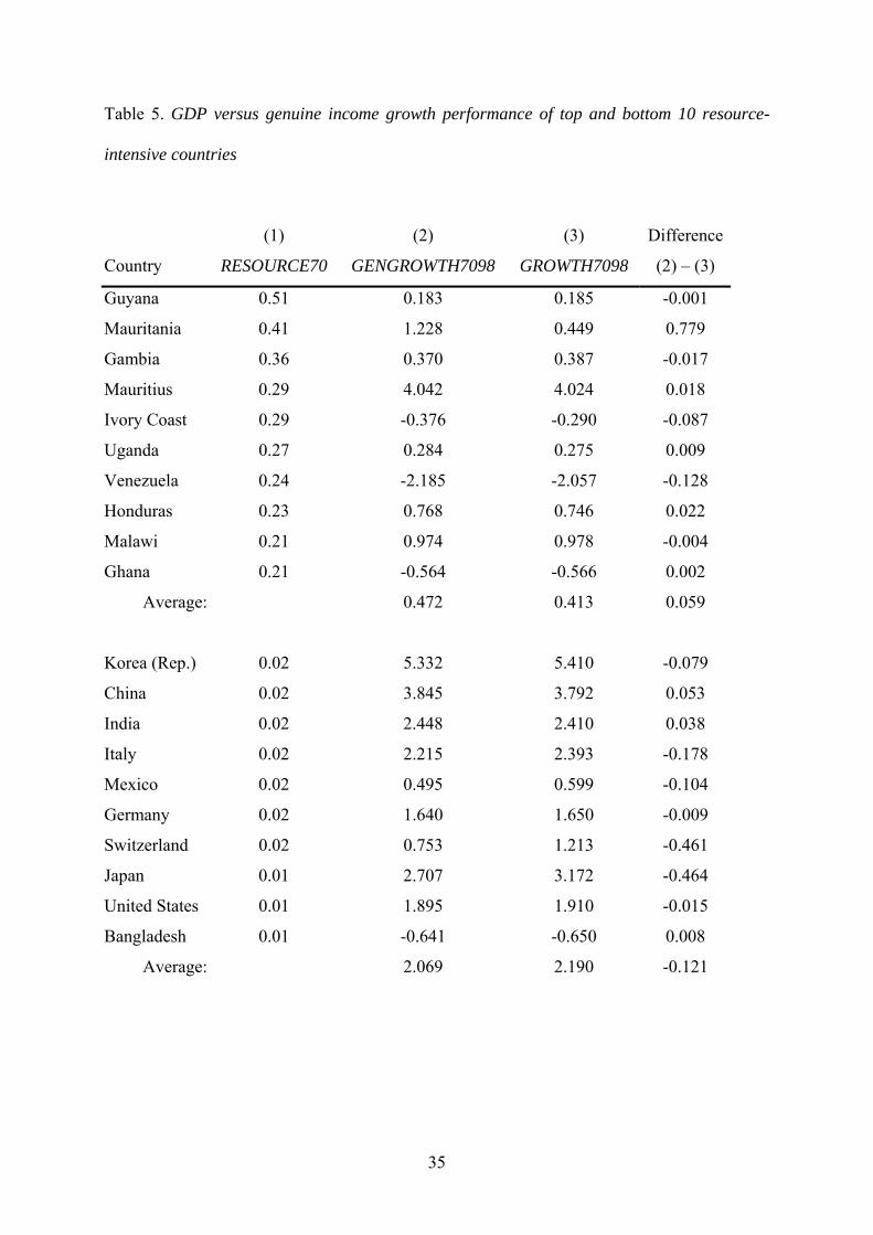
Let us illustrate the result that the ‘resource curse’ is not quite as strong in genuine
income as in GDP by showing the growth performance in GDP versus growth in
genuine income for the top and bottom 10 resource-intensive countries in our sample as
measured by RESOURCE70 (table 5). The very resource-intensive countries on average
have much lower GDP growth over the period 1970 to 1998 than the low resource-
intensive countries. However, on average their growth in genuine income is .06
percentage points higher than their GDP growth, whereas the growth in genuine income
of the 10 countries with the lowest resource-intensity is .12 percentage points lower than
their GDP growth.14 This illustrates nicely that the ‘resource curse’ is weaker in genuine
income, but a substantial gap in growth performance between the two groups of
countries pertains in genuine income as well.
< Insert Table 5 about here >
18
7. CONCLUSION
Our results can be summarized in two main propositions. First, natural resource-
intensive countries really do suffer from a ‘resource curse’. Existing studies have failed
to take into account natural capital depreciation and have analyzed growth of the wrong
term, namely GDP, instead of genuine income. In fact, looking at genuine income
instead reinforces the robustness of the evidence in favor of the ‘resource curse’.
Resource-intensive economies grow slower than their less resource-intensive peers in
terms of genuine income as well. Second, however, contrary to Mikesell’s (1997)
suggestion, the ‘resource curse’ is weaker in terms of growth of genuine income than
growth of GDP. Yet, the difference is small and in some estimations we cannot be sure
that it is statistically significantly different from zero. This therefore provides additional,
but somewhat weak and limited, evidence in support of those like Rodríguez and Sachs
(1999) and Atkinson and Hamilton (2003) who try to explain the poor performance of
natural resource-intensive economies with reference to unsustainable over-consumption.
For natural resource-intensive economies, GDP levels erroneously signal a level of
income that is beyond the sustainable level. It induces policy makers to engage in
excessive consumption and the country as a whole to living beyond its means. Genuine
income corrects GDP for what is truly capital depreciation rather than income. Once this
correction is done, we find that the ‘resource curse’ still holds, but it is weaker – as it
should be if unsustainable over-consumption is part of the explanation of the ‘curse’.
From the fact that the ‘resource curse’ still upholds if the growth performance is
measured in terms of genuine income levels and that the difference in estimated
coefficients is small and sometimes not statistically significantly different from zero
follows that explanations other than unsustainable over-consumption are required to
account for the bulk of the poor growth performance of natural resource-intensive
19
economies. Explaining the ‘resource curse’ therefore remains an important task for
future research by natural resource and development scholars.
What are the policy implications of our findings? Surely, leaving resources in the
ground is no solution. Rather, the challenge is to ensure that the revenues from natural
resource extraction are put to more productive use and the genuine savings rate is raised.
But how to achieve this? Discussing these issues thoroughly is beyond the scope of the
present article, so we will merely sketch some possibilities here without discussing their
merits and feasibility in any detail. Prudent fiscal policy, perhaps coupled with a natural
resource fund, can help to stabilize and sterilize some of the revenues. Multilateral
donors like the World Bank can require lenders to use some of the revenues for public
sector investment in health and education for the people rather than military and other
wasteful expenditures. This has been one of the major conclusions of the Bank’s
Extractive Industries Review (EIR), which was prompted by criticism from civil society
of the Bank’s role in financing natural resource projects (http://www.eireview.org).15
Some of the government-owned funds could be redistributed to citizens if governments
cannot be trusted to use the funds wisely. Careful exchange rate management can
mitigate the negative effects of resource booms on other sectors. Together these
measures could help stimulating investment in and diversification of the private sector.
However, these measures are of course difficult to achieve in countries plagued by poor
governance and bad institutional quality, which is typically the case in countries
affected by the ‘resource curse’. It is for this reason that in my view the political
economy approach that attempts to explain the poor growth performance with the
negative impact of natural resource wealth on the state of governance and institutional
quality represents the most promising path. On this aspect, Dietz, Neumayer and De
Soysa (2004) show that improving the quality of governance, particularly with respect
20
to corruption, reduces the negative impact of natural resource abundance on genuine
savings. Whilst not directly addressing the resource curse, these findings point toward
the importance of interaction effects between resource abundance and measures of
institutional quality.
In terms of future research, it would be worth while exploring using other model
specifications with growth in genuine income as the dependent variable. For example,
Stijns (2001a) and others have criticized Sachs and Warner’s (1997) measure of natural
resource intensity. Indeed, in using this measure there is a certain circularity in
argument since countries which successfully grow will reach a higher level of income
and therefore have a smaller natural resource exports to income ratio. Another problem
is that, depending on the country, the share of agriculture relative to minerals and fossil
fuels can be high in Sachs and Warner’s (1997) measure, whereas the ‘resource curse’
refers almost exclusively to mineral and fossil fuel extraction. It would be worthwhile
exploring alternative indicators of resource intensity, for example, a mineral and fossil
fuel rent indicator derived from the World Bank (2003) source used here to compute
genuine income. It would also be worth while checking if the ‘resource curse’ in
genuine income holds for alternative estimation techniques. Tackling these issues is
beyond the present paper’s scope, however.
21
NOTES
1 See, for example, Gelb and associates (1988) and Auty (1993).
2 See Stevens (2003) for a survey.
3 Also note that Roemer (1994) and others argue that Indonesia actually managed its oil
boom quite well via competent exchange rate management and a shift from inward-
looking to outward-looking policies.
4 Note, however, that Stijns (2001b) shows that if resource abundance is measured as
natural resource rents per capita, then economies with resource abundance do not have
lower education expenditures per capita.
5 Unfortunately, they do not report whether the negative growth effect of a low genuine
savings rate is stronger or weaker in resource intensive relative to resource poor
countries.
6 The same reasoning applies to renewable resources if harvesting exceeds natural
regeneration.
7 Neumayer (2000) is one of the very few studies applying the El Serafy method for a
range of countries.
8 Cuddington (1992) similarly finds non-uniformity in trends of 26 primary commodity
prices over the much longer period 1900 to 1983.
9 A reviewer wondered whether this variable and the LINV7098 variable described
further below should be altered in the estimations with growth in genuine income as the
dependent variable such that in their denominator GNP or GDP is replaced with genuine
income. However, this is not done here since the numerator of these variables is not
22
adjusted either. For example, the value of primary commodity exports is not adjusted
for natural capital depreciation and no sufficient data exist that would allow such
adjustment.
10 Such regressions are based on a neoclassical growth model. A reviewer raised the
question whether such regressions apply to genuine income at all, given that the
neoclassical growth model based on Solow (1956) assumes that a fixed share of national
income, not of genuine income, is saved and invested. To start with, there is nothing in
the Solow model that prevents it from being broadened to other forms of capital than
produced capital. Pender (1998), for example, includes natural capital in such a model.
Furthermore, the steady-state level in the Solow growth model is at the intersection of
investment and depreciation. Taking natural capital depreciation into account could
therefore be understood as raising depreciation, which would lower the steady-state
level of capital.
11 The data can be downloaded from World Bank (2003).
12 For details, see Bolt, Matete and Clemens (2002).
13 It is not clear whether this bias considerably affects our estimations and if so how. It
would represent much greater concern if we were to analyze differences in genuine
income levels rather than differences in genuine income growth. In any case, given the
lack of data on other items of natural capital, there is nothing that could be done about it
at this stage.
14 Note that this difference is not simply due to most countries in the upper panel being
developing countries and most countries in the lower panel being developed ones.
Australia and Canada, two classic examples of developed countries with a substantial
primary commodity sector (RESOURCE70 is .1 for both countries), also have slightly
23
higher genuine income than GDP growth (Australia: 1.69 versus 1.66; Canada: 1.92
versus 1.79).
15 World Bank lending to Chad for the development of an oil pipeline is an example
where the Bank has at least tried to pressure the lending government into using parts of
the funds in a non-corrupt, transparent way that is beneficial to health care and rural
development.
24
REFERENCES
Atkinson, G., & Hamilton, K. (2003). Savings, growth and the resource curse
hypothesis. World Development, 31, 1793-1807.
Auty, R.M. (1993). Sustaining development in mineral economies. London: Routledge.
Auty, R.M. (1994). Industrial policy reform in six large newly industrializing countries:
the resource curse thesis. World Development, 22, 11-26.
Auty, R.M. (ed) (2001). Resource abundance and economic development. Oxford:
Oxford University Press.
Auty, R.M., & Mikesell, R.F. (1998). Sustainable development in mineral economies.
Oxford: Clarendon Press.
Belsley, D.A., Kuh, E., & Welsch, R.E. (1980). Regression Diagnostics. New York:
John Wiley.
Bolt, K., Matete, M., & Clemens, M. (2002). Manual for Calculating Adjusted Net
Savings. Washington, DC: World Bank.
Cuddington, J.T. (1992). Long-run trends in 26 primary commodity prices. Journal of
Development Economics, 39, 207-227.
Davis, G.A. (1995). Learning to love the Dutch disease: evidence from the mineral
economies. World Development, 23, 1765-1779.
Dietz, S., Neumayer, E., & De Soysa, I. (2004). Corruption, the Resource Curse and
Genuine Savings. Mimeo. London: London School of Economics.
El Serafy, S. (1981). Absorptive Capacity, the Demand for Revenue, and the Supply of
Petroleum, Journal of Energy and Development, 7, 73-88.
25
El Serafy, S. (1989). The proper calculation of income from depletable natural
resources. In Y.J. Ahmad, S. El Serafy, & E. Lutz (Eds.): Environmental accounting
for sustainable development: A UNDP-World Bank symposium, (pp. 10-18),
Washington, DC: World Bank.
Gallup, J.L, Sachs, J.D., & Mellinger, A.D. (1999). Geography and economic
development. In B. Pleskovic, & J.E. Stiglitz (Eds.): Annual World Bank Conference
on Development Economics 1998, (pp. 127-172), Washington, DC: World Bank.
Gelb, A.H. and associates (1988). Oil winfalls: blessing or curse? New York: Oxford
University Press.
Gylfason, T. (2001). Nature, power and growth. Scottish Journal of Political Economy,
48, 558-588
Gylfason, T., & Zoega, G. (2002). Natural resources and economic growth: the role of
investment. Working Paper No. 142. Santiago de Chile: Central Bank of Chile.
Hamilton, K. (1996). Pollution and Pollution Abatement in the National Accounts.
Review of Income and Wealth, 42, 13-33.
Hartwick, J.M. (1977). Intergenerational Equity and the Investing of Rents from
Exhaustible Resources. American Economic Review, 67, 972-974.
Hartwick, J.M., & Hageman, A. (1993). Economic Depreciation of Mineral Stocks and
the Contribution of El Serafy. In Ernst Lutz (Ed.): Toward Improved Accounting for
the Environment, (pp. 211-235), Washington, DC: World Bank.
Heston, A., Summers, R., & Aten, B. (2002). Penn World Tables Version 6.1. Center
for International Comparisons at the University of Pennsylvania.
26
Hotelling, H. (1931). The Economics of Exhaustible Resources, Journal of Political
Economy, 39, 137-175.
Isham, J., Woolcock, M., Pritchett, L., & Busby, G. (2003). The varieties of resource
experience: How natural resource export structures affect the political economy of
economic growth. Economics Discussion Paper No. 03-08. Middlebury College.
Lal, D., & Myint, H. (1996). The political economy of poverty, equity and growth.
Oxford: Clarendon Press.
Maloney, W.F. (2001). Innovation and growth in resource rich countries. Working
Paper 148. Santiago de Chile: Central Bank of Chile.
Manzano, O., & Rigobon, R. (2001). Resource curse or debt overhang? Working Paper
8390. Cambridge (Mass.): National Bureau of Economic Research.
Mikesell, R.F. (1997). Explaining the resource curse, with special reference to mineral-
exporting countries. Resources Policy, 23, 191-199.
Neumayer, E. (2000). Resource accounting in measures of unsustainability: Challenging
the World Bank’s conclusions. Environmental and Resource Economics, 15, 257-278.
Neumayer, E. (2003). Weak versus Strong Sustainability: Exploring the Limits of Two
Opposing Paradigms. Second Revised Edition. Cheltenham: Edward Elgar.
Pender, J.L. (1998). Population growth, agricultural intensification, induced innovation
and natural resource sustainability: an application of neoclassical growth theory.
Agricultural Economics, 19, 99-112.
Prebisch, R. (1950). The economic development of Latin America and its principal
problems. Lake Success, NY: United Nations.
27
Repetto, R., Magrath, W., Wells, M., Beer, C., & Rossini, F. (1989). Wasting Assets:
Natural Resources in the National Income Accounts. Washington, DC: World
Resources Institute.
Rodríguez, F., & Sachs, J.D. (1999). Why do resource abundant economies grow more
slowly? A new explanation and an application to Venezuela. Journal of Economic
Growth, 4, 277-303.
Roemer, M. (1994). Dutch disease and economic growth: the legacy of Indonesia.
Development Discussion Paper No. 489. Cambridge (Mass.): Harvard Institute for
Development Research.
Ross, M.L. (1999). The political economy of the resource curse. World Politics, 51,
297-322.
Sachs, J.D., & Warner, A.M. (1995a, 1997). Natural resource abundance and economic
growth. Working Paper 5398. Cambridge, MA: National Bureau of Economic
Research and Harvard University.
Sachs, J.D., & Warner, A.M. (1995b). Economic reform and the process of global
integration. Brookings Papers on Economic Activity, 1, 1-118.
Sachs, J.D., & Warner, A.M. (2001). The curse of natural resources. European
Economic Review, 45, 827-838.
Sala-i-Martin, X., & Subramanian, A. (2003). Addressing the natural resource curse:
An illustration from Nigeria. Working Paper 9804. Cambridge, MA: National Bureau
of Economic Research.
Santopietro, G.D. (1998). Alternative Methods for Estimating Resource Rent and
Depletion Cost: the Case of Argentina’s YPF. Resources Policy, 24, 39-48.
28
Serôa da Motta, R., & Ferraz do Amaral, C.A. (2000). Estimating Timber Depreciation
in the Brazilian Amazon. Environment and Development Economics, 5, 129-142.
Serôa da Motta, R., & Young, C. (1995). Measuring sustainable income from mineral
extraction in Brazil. Resources Policy, 21, 113-125.
Shihata, I. (1982). The Other Face of OPEC—Financial Assistance to the Third World.
London and New York: Longman.
Solow, R. (1956). A contribution to the theory of economic growth. Quarterly Journal
of Economics, 70, 65-94.
Stauffer, T.R., & Lennox, F.H. (1984). Accounting for ‘wasting assets’ – income
measurement for oil and mineral-exporting rentier states. Vienna: OPEC Fund for
International Development.
Stevens, P. (2003). Resource impact – curse or blessing? A literature survey. University
of Dundee.
Stijns, J-P. (2001a). Natural resource abundance and economic growth revisited.
University of California at Berkeley.
Stijns, J-P. (2001b). Natural resource abundance and human capital accumulation.
Working paper. University of California at Berkeley.
Vincent, J.R. (1997). Resource Depletion and Economic Sustainability in Malaysia,
Environment and Development Economics, 2, 19-37.
Winter-Nelson, A. (1995). Natural resources, national income, and economic growth in
Africa. World Development, 23, 1507-1519.
World Bank (2001). World Development Indicators on CD-Rom. Washington, DC:
World Bank
29
World Bank (2003). Green Accounting and Adjusted Net Savings website.
http://lnweb18.worldbank.org/ESSD/envext.nsf/44ByDocName/GreenAccountingAdj
ustedNetSavingsT. accessed on 19 January 2004
30
Table 1. The difference between net price method and El Serafy method
n / r 1% 2% 3% 4% 5% 10%
5 5.80 11.20 16.25 20.97 25.38 43.55
10 10.37 19.57 27.76 35.04 41.53 64.95
15 14.72 27.16 37.68 46.61 54.19 78.24
20 18.86 34.02 46.25 56.12 64.11 86.49
30 26.54 45.88 60.00 70.35 77.96 94.79
50 39.80 63.58 77.85 86.47 91.69 99.23
100 63.39 86.47 94.95 98.10 99.28 99.99
Note: Table shows difference between net price method (equation (2)) and El Serafy
method (equation (3)) for a value of $100 according to equation (2). n is the number of
remaining years of the resource stock and r is the discount rate.
31
Table 2. Change in average resource prices over the period 1970 to 1998 (Index 1970
= 100)
1970 1980 1990 1998
bauxite 100 134.55 95.40 55.86
copper 100 82.79 66.22 34.77
gold 100 859.97 355.09 228.61
hard coal 100 222.59 147.10 104.59
iron ore 100 104.86 76.86 62.82
lead 100 136.58 95.60 80.41
lignite 100 222.72 147.18 104.13
natural gas 100 211.08 120.04 76.65
nickel 100 118.27 104.60 46.06
oil 100 885.74 367.19 173.84
phosphate rock 100 197.24 122.53 106.64
silver 100 586.43 90.61 87.27
tin 100 231.16 56.60 42.07
zinc 100 123.34 162.27 92.55
Source: World Bank (2003), converted into 1985 prices with the help of the US GDP
deflator, taken from World Bank (2001).
32
Table 3. Estimation results (absolute t-values in parentheses)
(1a) (2a) (3a) (4a) (5a) (1b) (2b) (3b) (4b) (5b)Dep. Variable: GROWTH
7098 GROWTH
7098 GROWTH
7098 GROWTH
7098 GROWTH
7098 GENGROWTH
7098 GENGROWTH
7098 GENGROWTH
7098 GENGROWTH
7098 GENGROWTH
7098 LGDP70 0.078 -0.542 -0.813 -0.855 -0.843
(0.46) (2.94)** (3.92)** (3.75)** (3.66)**LGENINC70 -0.001 -0.614 -0.879 -0.912 -0.896 (0.01) (3.26)** (4.14)** (3.92)** (3.83)**RESOURCE70 -5.576 -4.107 -3.502 -5.262 -5.383 -5.048 -3.630 -3.061 -5.060 -5.206 (3.15)** (2.67)** (2.33)*
(3.10)**
(3.14)**
(2.84)** (2.34)* (2.01)* (2.96)** (3.02)**
OPEN7090 2.206 1.979 1.596 1.594 2.159 1.931 1.551 1.549 (5.62)** (5.07)** (3.28)**
(3.27)**
(5.49)** (4.91)** (3.17)** (3.16)**
LINV7098 0.773 0.726 0.755 0.750 0.706 0.741 (2.55)* (2.31)* (2.37)*
(2.46)* (2.24)* (2.31)*
RULE8295 0.063 0.051 0.052 0.037 (0.46) (0.37) (0.38) (0.27)TTGROWTH7098
-0.051 -0.061(0.62) (0.74)
Constant
1.457 5.624 5.904 6.511 6.371 2.022 6.115 6.394 6.972 6.801(0.97) (3.78)**
(4.09)**
(4.18)**
(4.03)**
(1.32) (4.04)** (4.34)** (4.40)** (4.23)**
Observations 86 86 86 79 79 86 86 86 79 79R-squared 0.12 0.37 0.41 0.42 0.43 0.09 0.34 0.38 0.40 0.41
* significant .05 level ** at .01 level.
33
Table 4. Tests of equality for coefficients of the natural resource-intensity variable
Regression: (1) (2) (3) (4) (5)
Non-standardized coefficients:
Dep. Var.: GROWTH7098 -5.576 -4.107 -3.502 -5.262 -5.383
Dep. Var.: GENGROWTH7098 -5.048 -3.630 -3.061 -5.060 -5.206
χ2 test equality of coefficients
(p-value)
3.62
(.0571)
3.18
(.0743)
3.15
(.0758)
2.58
(.1085)
2.01
(.1562)
Standardized beta coefficients:
Dep. Var.: GROWTH7098 -.335 -.247 -.210 -.299 -.306
Dep. Var.: GENGROWTH7098 -.307 -.221 -.186 -.291 -.299
χ2 test equality of coefficients
(p-value)
2.59
(.1078)
3.41
(.0650)
3.81
(.0509)
1.68
(.1947)
1.18
(.2766)
34
Table 5. GDP versus genuine income growth performance of top and bottom 10 resource-
intensive countries
Country
(1)
RESOURCE70
(2)
GENGROWTH7098
(3)
GROWTH7098
Difference
(2) – (3)
Guyana 0.51 0.183 0.185 -0.001
Mauritania 0.41 1.228 0.449 0.779
Gambia 0.36 0.370 0.387 -0.017
Mauritius 0.29 4.042 4.024 0.018
Ivory Coast 0.29 -0.376 -0.290 -0.087
Uganda 0.27 0.284 0.275 0.009
Venezuela 0.24 -2.185 -2.057 -0.128
Honduras 0.23 0.768 0.746 0.022
Malawi 0.21 0.974 0.978 -0.004
Ghana 0.21 -0.564 -0.566 0.002
Average: 0.472 0.413 0.059
Korea (Rep.) 0.02 5.332 5.410 -0.079
China 0.02 3.845 3.792 0.053
India 0.02 2.448 2.410 0.038
Italy 0.02 2.215 2.393 -0.178
Mexico 0.02 0.495 0.599 -0.104
Germany 0.02 1.640 1.650 -0.009
Switzerland 0.02 0.753 1.213 -0.461
Japan 0.01 2.707 3.172 -0.464
United States 0.01 1.895 1.910 -0.015
Bangladesh 0.01 -0.641 -0.650 0.008
Average: 2.069 2.190 -0.121
35
APPENDIX 1: DERIVATION OF USER COSTS ACCORDING TO
THE EL SERAFY METHOD
The formula for computing user costs according to the El Serafy method can be derived as
follows: Let P be the resource price, AC average extraction cost, R the amount of resource
extracted, r the discount rate and n the number of remaining years of the resource stock if
extraction was the same in the future as in the base year, i.e. n is the static reserves to
extraction ratio. Then the present value of total resource rents RR ≡ (P-AC)⋅R is equal to:
r
rRR
rRR nn
i i
+−
⎥⎥⎦
⎤
⎢⎢⎣
⎡
+−
=∑+
+
=
111
)1(11
)1(
1
0 (1)
The present value of an infinite stream of ‘sustainable income’ SI is
r
SIr
rSIr
SIi i
+−
=+
=∑+
∞
=
111
)1()1(0
(2)
Setting (1) and (2) equal and rearranging expresses SI as a fraction of RR:
⎥⎥⎦
⎤
⎢⎢⎣
⎡
+−=
+)1(11 1r
RRSI n
The user costs, representing the depreciation of the resource stock, would thus be
⎥⎥⎦
⎤
⎢⎢⎣
⎡
+⋅−=
⎥⎥⎦
⎤
⎢⎢⎣
⎡
+=−
++ )1(1)(
)1(1)( 11 r
RACPr
RRSIRR nn
36
APPENDIX 2: VARIABLE DEFINITION AND SOURCES OF DATA
LGDP70: Natural log of real purchasing power parity adjusted GDP in 1970 divided by
the economically-active population in 1970. Economically active population is defined as
population aged 15 to 64. GDP is converted into 1985 prices with the help of the US GDP
deflator (Sachs and Warner’s (1997) original analysis is in 1985 prices). Source: Heston,
Summers and Aten (2002) for GDP (rgdpch series), World Bank (2001) for population
data and the US GDP deflator.
LGENINC70: Natural log of real purchasing power parity adjusted genuine income in
1970 divided by the economically-active population in 1970. Economically active
population is defined as population aged 15 to 64. Genuine income is defined as GDP
minus depreciation of produced and natural capital stocks. Data for depreciation of
produced capital are originally derived from United Nations Statistics Division.
Depreciation of natural capital covers oil, gas, coal, bauxite, copper, iron ore, lead, nickel,
phosphate rock, tin, zinc, gold and silver and is computed according to net price method
(see text for details). Both GDP and depreciation data converted into 1985 prices with the
help of the US GDP deflator. Source: Heston, Summers and Aten (2002) for GDP (rgdpch
series), World Bank (2001) for population data and the US GDP deflator and World Bank
(2003) for depreciation data.
GROWTH7098: Real per capita GDP growth rate per annum computed as
100*(1/28)*(LGDP98-LGDP70), where LGDP98 is defined as LGDP70, but for 1998.
Source: Heston, Summers and Aten (2002).
GENGROWTH7098: Real per capita genuine income growth rate per annum computed as
100*(1/28)*(LGENINC98-LGENINC70), where LGENINC98 is defined as LGENINC70,
but for 1998. Source: Heston, Summers and Aten (2002) and World Bank (2003).
37
RESOURCE70: Share of exports of primary products in GNP in 1970. Primary products
cover agricultural, mineral and fuel products. Source: Sachs and Warner (1997) who
derive their data from World Bank: World Data 1995 CD-Rom. Sachs and Warner make a
number of amendments to this variable, see Sachs and Warner (1997, p. 29) for details.
OPEN7090: Fraction of years a country is rated as an open economy during the period
1970 to 1990. Source: Sachs and Warner (1995b).
LINV7098: Natural log of real gross domestic investment to real GDP, averaged over the
period 1970 to 1998. Source: Heston, Summers and Aten (2002) (rgdpl series).
RULE8295: An index of the quality of the rule of law, averaged over the period 1982 to
1995. The index runs on a 0 (worst) to 6 (best) scale and is defined as ‘respect for law and
order, predictability and effectiveness of the judiciary system, enforceability of contracts’.
Source: International Country Risk Guide, published by Political Risk Services
(www.icrgonline.com).
TTGROWTH7098: Average annual growth in the log of the external terms of trade
between 1970 and 1998. It is computed as 100*(1/28)*(ln(TT1998)-ln(TT1970)), where
TT means terms of trade and is defined as the ratio of an export price index to an import
price index with base year 1995 (note: re-basing to 1985 not necessary). Source: World
Bank (2001).
38