World tariff liberalization in agriculture: an … tariff liberalization in agriculture: an...

Research PapersIssue RP0223June 2014

CIP - Climate Impactsand Policy Division

World tariff liberalization inagriculture: an assessment followinga global CGE trade model for EU15regions

By Gabriele StandardiFondazione Eni Enrico Mattei

(FEEM),Centro Euro-Mediterraneo sui

Cambiamenti Climatici (CMCC)[email protected]

Federico PeraliUniversity of Verona,

Department of EconomicSciences

Luca PieroniUniversity of Perugia,

Department of Economics,Finance and Statistics

SUMMARY This paper aims at modeling a global CGE trade model for theEU15 subnational regions. This model is used to assess productionreallocation across sectors in each EU15 region, assuming a scenario inwhich world tariff liberalization is implemented in the agricultural sector. Themodel is parsimonious in terms of data, focusing on unskilled and skilledlabor as the source of heterogeneity across regions. A stylized model isbuilt to interpret trade policy effects. Results show decreases in agriculturalproduction in the EU15 of about 0.93%. All regions reduce agriculture butshow different magnitudes in the relative changes of production. Largereallocation effects are observed between manufactures and services,some regions specializing in the former and others in the latter. In addition,the introduction of labor mobility within the EU15 and the EU27 causesstrong amplification effects in manufactures and services.

Keywords: CGE modeling, International trade, Agriculture

JEL: F13, D58, Q17

CMCC Research Papers

02

Cen

tro

Euro

-Med

iterr

aneo

sui

Cam

biam

enti

Clim

atic

i

1. INTRODUCTION In recent years the development of the World Trade Organization (WTO) has generated

great demand for estimating the potential consequences of trade policy. The Uruguay and

Doha rounds of negotiations are typical examples. As a consequence, policy-makers are

interested in obtaining information about the effects of trade liberalization on income,

production and other important macro-economic variables. It is especially useful to know

something about the distribution of these effects across families, countries or sectors, to

evaluate who are the winners and who the losers.

Computable General Equilibrium (CGE) global trade models, such as GTAP (Hertel,

1997), MEGABARE (Hanslow and Hinchy, 1996) and MIRAGE (Bchir et al., 2002) are

important tools for meeting this need.1 Unfortunately, these kinds of models characterize

analysis at national level and there is little literature assessing the consequences of trade

policies at subnational level. Nevertheless, knowledge about disaggregated geographical

effects may add value for policy-makers. This is because trade liberalization involves strong

distributional effects, not only across sectors or countries but also across the regions of a

given country. In addition, the EU economy is highly diversified and world trade agreements

do not take into account the disparities existing at regional level. As an implicit statement,

this geographical heterogeneity in the EU should be considered in WTO negotiations.

The aim of this work is to build a global CGE trade model at NUTS 1 (Nomenclature of

Territorial Units for Statistics) level for the 68 regions within the first 15 member states of

the European Union. This type of model should allow the consequences of trade policy in

Europe to be investigated at a disaggregated geographical level while maintaining a global

approach.2 The model is used to analyze the output reallocation across sectors in each

NUTS 1 region after multilateral tariff liberalization in agriculture. Unskilled and skilled labor

reallocation across regions is also analyzed.

The proposed simulation does not attempt to reproduce exactly the policies discussed in

the current Doha round. For market access in the agricultural sector, the definition of tariff

1 GTAP is the acronyms for Global Trade Analysis Project. The MEGABARE model was developed by

ABARE (Australian Bureau of Agricultural and Resources Economics). MIRAGE stands for Modelling International Relationships in Applied General Equilibrium, and was developed by CEPII (Centre d’Etudes Prospectives et d’Informations Internationales).

2 The Nomenclature of Territorial Units for Statistics is a subnational geocode standard developed by the European Union for referencing subdivisions of European countries for statistical purposes. There are three levels of aggregation: level 1 (more aggregated), level 2 (medium aggregated) and level 3 (less aggregated).

World tariff liberalization in agriculture: an assessment following a global CGE trade model for EU15 regions

03

Cen

tro

Euro

-Med

iterr

aneo

sui

Cam

biam

enti

Clim

atic

i

reductions involves highly technical issues, such as formula adopted for cuts, definition of

“sensitive products” (which are partially excluded from general tariff reductions) and

commitments for developing countries (Anania and Bureau, 2005). The main aim of this

model is to shed light on possible outcomes of global trade liberalization at NUTS 1 level,

outcomes which have been little explored in the literature.

Our results show that all the NUTS 1 regions decrease agricultural production after world

tariff liberalization in the sector. However, some regions are more affected than others. In

manufactures and services, inverse patterns of production changes at NUTS 1 level are

noted; some regions showing strong decreases in the first sector and strong increases in

the second one, while other regions experience decreases in the latter and increases in the

former. The assumption of labor mobility has a huge impact on this reallocation process

between manufactures and services. Lastly, we find that welfare gains are limited for the

world as a whole and almost insignificant for Europe. The paper is organized as follows. Section 2 presents the relevant literature for CGE

trade models at subnational level. Section 3 describes data and the calibration strategy.

Section 4 illustrates the chosen sectoral and geographical aggregations and the trade

policy simulation. Section 5 sets out the structure of the model and subsection 5.1 the

associated stylized model used to clarify trade policy effects. Section 6 shows the results of

the trade policy simulation. Section 7 explains policy implications and makes some

concluding remarks.


04

Cen

tro

Euro

-Med

iterr

aneo

sui

Cam

biam

enti

Clim

atic

i

2. RELEVANT LITERATURE FOR CGE TRADE MODELS AT SUBNATIONAL LEVEL

Our approach is related to other studies concerning global CGE trade models at

subnational level. It is worth noting that CGE trade models exist at subnational level, but

they only consider a single region or few regions. The MONASH-MRF (Peter et al., 1996),

CAPRI-GTAP (Jansson, Kuiper and Adenäuer, 2009), GTAP-CAPSiM (Yang et al., 2011)

and MIRAGE-DREAM (Jean and Laborde, 2004) models are examples of large-scale

global CGE trade models, which also include many regions.3 Australia, in particular, has a

strong tradition of this type of model, and MONASH-MRF has been applied to several policy

issues concerning not only trade but also environmental economics.4 MIRAGE-DREAM

considers the NUTS regions of the 25 members of the EU. CAPRI-GTAP and CAPSiM are

specific to the European and Chinese agricultural sectors.

In the economic literature, there are few models at subnational level because of the lack

of well-suited subnational data on foreign trade. For instance, the EU has no complete

dataset on foreign trade which is available for the NUTS regions. Concerning foreign trade,

some information is available for some countries at regional level, but this is not

systematically the case. Thus, simplifying assumptions must be made to make the models

manageable.

Our approach is similar to that used by Jean and Laborde (2004) in the MIRAGE-

DREAM model, which contains a NUTS 1 representative regional household as well as a

NUTS 1 representative regional firm. As a result, the model is very demanding, in both

terms of data and computational resources. However, the lack of well-suited data

concerning trade across NUTS 1 regions and between NUTS 1 regions and countries

outside Europe makes it necessary to resort to simplifying assumptions.

In contrast, we have built a parsimonious CGE model, which uses relatively little

information at NUTS 1 level, i.e., value added, and skilled and unskilled labor. Only the

production side is considered at NUTS 1 level. In each NUTS 1 region, a representative

firm maximizes profits. Simplifying assumptions are made for all the variables of production

other than value added, skilled and unskilled labor. The demand side is specified at EU15

level. This means that imports, exports and domestic demand, as well as their associated

3 CAPRI is an acronym for Common Agricultural Policy Regional Impact Analysis. The MONASH-MRF model was developed at Monash University. MRF stands for Multi-Regional Forecasting, DREAM stands for Deep Regional Economic Analysis Model, and CAPSiM is China’s Agricultural Policy Simulation Model.

4 See Horridge et al. (2005) for an application of the MONASH-MRF model to the 2002-2003 drought in Australia.


05

Cen

tro

Euro

-Med

iterr

aneo

sui

Cam

biam

enti

Clim

atic

i

prices, are at EU15 level (for example, the price of good, paid by the EU15 representative

household, is the same in all NUTS 1 regions).

A major limitation of CGE models is poor economic interpretation of trade policy effects

because of many variables and equations, which make them a “black box” (Panagariya and

Duttagupta, 2001). For this reason and in line with other works, we build a stylized model

which reproduces the main features of our model, in order to better understand the

underlying economic functioning.5 This interpretation is based on the ratio between

unskilled and skilled labor intensity, because these are the two factors which may be

considered as the source of heterogeneity at NUTS 1 level, since they are the only two

primary factors for which data are available at this level.

Finally a sensitivity analysis is conducted to test the relevance of the assumption about

skilled/unskilled labor mobility within the Europe.

3. DATA AND CALIBRATION STRATEGY

In order to carry out analysis at a disaggregated geographical level, we match two

different databases: one national and the other subnational. The national one is GTAP 6

(Dimaranan and Mac Dougall, 2005), a large social accounting matrix (SAM) for 87

countries or groups of countries and 57 sectors. It contains information on bilateral trade

flows and transports linkages among countries. The base-year for the GTAP 6 version is

2001. It also incorporates the MAcMap database for tariff barriers (Bouet et al., 2004).6

The subnational database is derived from EUROSTAT. We draw on the methodology

used by Laborde and Valin (2007) to obtain value added, skilled and unskilled labor at

NUTS 1 level. Laborde and Valin use EUROSTAT tables, which consider 247 NUTS 2

regions in EU25 (data not available for Bulgaria and Romania).7 Most of the EUROSTAT

data are from 2003, which is the most recent year which had the smallest number of

missing values. However, when no data is available for 2003, data from 2001 and 2002 are

used.

5 Adams (2005) built a stylized model to interpret the results form CGE models such as GTAP. 6 MAcMap is the most comprehensive tariff database currently available. It was expressly created for CGE

trade models and provides a good measure of market access. This measure is a consistent ad valorem equivalent of specific tariffs, ad valorem tariffs and tariff quotas. This dataset also greatly allows for preferential agreements preserving information at bilateral level. Before the creation of the MAcMap database, assessment of multilateral trade policy liberalization was carried out without taking into account specific tariffs or preferential agreements.

7 It should be noted that some missing values occur in the EUROSTAT tables. Filling methods were applied with other complementary tables from EUROSTAT and GTAP information (see Laborde and Valin, 2007).


06

Cen

tro

Euro

-Med

iterr

aneo

sui

Cam

biam

enti

Clim

atic

i

To summarize, we can use a national database (GTAP 6) with 87 countries or groups of

countries and 57 sectors, and a subnational database (EUROSTAT) with 247 NUTS 2

regions and 39 NACE sectors.8

The calibration strategy for production variables other than value added (VA), unskilled

labor (L) and skilled labor (H) was to resort to simplifying assumptions. The repartition key

of value added at NUTS 1 level is used to regionalize the other production variables,

according to the following formulas:

,,

, 15

,i ri r

i EU

VAKEYVA

VA= (1)

, , , 15 ,i r i r i EUTE KEYVA TE= ⋅ (2)

, , , 15 ,i r i r i EURN KEYVA RN= ⋅ (3) , , , 15 ,i r i r i EUK KEYVA K= ⋅ (4)

, , , , , 15 ,j i r i r j i EUINI KEYVA INI= ⋅ (5)

where i and j are sector indexes, r is the region index and KEYVA is the repartition key of

value added; TE, RN, K and INI are, respectively, land, natural resources, capital and

intermediate inputs (sold by sector j to sector i).

It is reasonable to think that a greater value added in the NUTS 1 region means greater

use of primary factors and intermediate inputs. This hypothesis neglects the fact that two

NUTS 1 regions, equal in terms of factor endowments, can use primary factors and

intermediate inputs through different intensities, i.e. they may have different technologies.

Data constraints forced us to make this choice. Thus, the factors skilled and unskilled labor

are the only two which preserve their original heterogeneity at NUTS 1 level. Section 5.1

shows that they are decisive in explaining trade policy effects.

All parameters are calibrated to reproduce SAM in the base-year (2001). Most of them

can be directly determined through the available data. However, for some of them, such as

as CES (constant elasticity of substitution) elasticities, this operation is not feasible and we

therefore explicitly refer to the latest version of the MIRAGE model (Decreux and Valin,

2007) which, in turn, draws elasticities from empirical literature or plausible assumptions.

8 39 sectors are a compromise, based on various EUROSTAT tables which were used in addition to the

GTAP information incorporated into the NUTS 2 dataset.


07

Cen

tro

Euro

-Med

iterr

aneo

sui

Cam

biam

enti

Clim

atic

i

Concerning the elasticity of unskilled migration (σL) and that of skilled migration (σH) in

the CET (constant elasticity of transformation) functions, which determine unskilled and

skilled labor supplies in each NUTS 1 region, we carry out a sensitivity analysis to test the

relevance of these two parameters for trade policy results. The two parameters can assume

two different values (zero or ten) according to the simulated labor market scenario: perfect

immobility at NUTS 1 level (σL = σH = 0), high mobility within the EU15 (σL = σH = 10) and

high mobility within the EU27 (σL = σH = 10).9 In the MIRAGE-DREAM model, Jean and

Laborde (2004) used elasticity of migration based on the work of Eichengreen (1993).10

9 In the last scenario, the rest of Europe is considered as a single region and added to the 68 NUTS 1

regions in the EU15 to form an integrated labor market. 10 Eichengreen draws the value of this parameter from data for the United Kingdom and Italy, and no

distinction is made between unskilled and skilled labor. To the best of our knowledge, no specific econometric estimates exist to calibrate the unskilled/skilled elasticity of migration for the EU15 and EU27 in CGE models.


08

Cen

tro

Euro

-Med

iterr

aneo

sui

Cam

biam

enti

Clim

atic

i

4. SECTORAL AND GEOGRAPHICAL AGGREGATIONS AND TRADE POLICY SIMULATIONS

This section sets out the sectoral and geographical aggregations chosen for the model

and the trade policy simulation. Two levels define geographical aggregation: one for macro-

areas and the other for the 68 NUTS 1 regions in the EU15. The first level is used to define

demand side variables. There are three macro-areas: the EU15, the rest of Europe (REU)

and the rest of the world (ROW). We distinguish between the EU15 and the REU because

the EUROSTAT database is more precise for the first 15 members of the EU. In addition,

Bulgaria and Romania do not figure in the NUTS database. Lastly, it is reasonable to think

of EU15 and REU as more homogenous economic macro-areas. The second geographical

level is used to define production side variables. There are 68 NUTS 1 regions within EU15.

ROW and REU production variables continue to be defined at the first geographical level.

There are four sectors for sectoral aggregation. A small number of sectors is preferable,

because our aim is not to assess trade policy effects with respect to any specific sector, but

rather to understand the general equilibrium effects of production reallocation across NUTS

1 regions. Tables 1, 2 and 3 display chosen aggregations.

We focus on market access measures and put aside the other two pillars of trade

agreements, export subsidies and domestic support. This is for two reasons. First, we wish

to preserve the simplicity of the model in order to be able to interpret its outcomes better at

NUTS 1 level. Second, the role of export subsidies and domestic supports in agricultural

trade liberalization does not seem to be very important. Hertel and Keeney (2006) simulate

full liberalization of the agricultural sector by high-income countries with the GTAP model.

More than 90% of the benefits come from improved market access, i.e., removal of ad

valorem equivalent tariffs, whereas the influence of domestic support and export subsidies

is limited.

We use the 2004 version of MAcMap, which is incorporated in the GTAP 6 database; the

base-year is 2001. Thus, baseline equilibrium, in which trade liberalization is implemented,

does not consider as achieved either European enlargement or other commitments which

had taken place by the end of 2004 (e.g., China's accession to the WTO).

According to the MAcMap database and its ad valorem equivalent measure, market

access was the following in 2001. Agriculture was the most highly protected sector. The

world average is 19.1%. Average agricultural protection ranges from 2.7% in Australia to


09

Cen

tro

Euro

-Med

iterr

aneo

sui

Cam

biam

enti

Clim

atic

i

59.6% in India. Manufacturing products apart from textiles and apparel are the least

protected sector on average (4.2%). However, tariffs are low in developed countries but

remain high in developing ones. Tariffs in the textile and apparel sectors are also high, in

both developed and developing countries. Services market access is a problematic

concept, since explicit tariffs do not exist. Equivalent tariffs for services are sometimes

estimated with gravity equations.

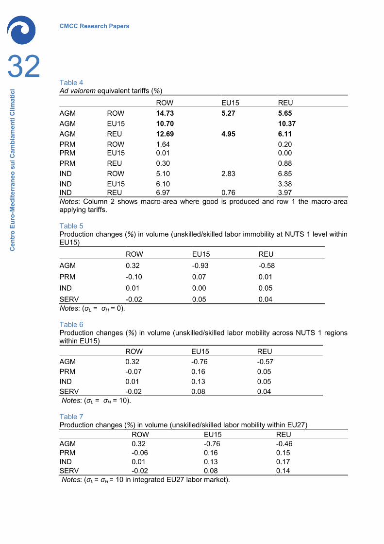
Table 4 shows ad valorem equivalent tariff rates for the geographical and sectoral

nomenclature chosen in our model. Basically, the parameter enters the demand side with

the following equation:

( ), , ' , , , '1 ,i m m i m i m mPDEM PY ATR= ⋅ + (6)

where PDEM is the price for good i produced in macro-area m and paid for by macro-area

m’, PY is the price (marginal cost) for good i produced in macro-area m and parameter ATR

is the ad valorem equivalent tariff rate applied by macro-area m’ on the good produced in

the macro-area m. Table 4 confirms the previous facts about trade barriers.11 We decide to

implement multilateral tariff liberalization in agriculture, and all the ad valorem tariff rates

are set at zero in the agricultural sector for all macro-areas (values in bold type in Table 4).

11 Not surprisingly, tariff barriers appear between EU15 and the rest of Europe, as 12 countries were not

European members in 2001.


10

Cen

tro

Euro

-Med

iterr

aneo

sui

Cam

biam

enti

Clim

atic

i

5. STRUCTURE OF THE MODEL

As stated above, the model considers two levels of geographical aggregation. The first

contains three macro-areas (EU15, rest of Europe, rest of the world) and the second the 68

NUTS 1 regions. Sectoral aggregation is the same in the two levels.

All demand variables are defined at macro-area level, implying that the price of each

demand variable is equal in all NUTS 1 regions. Unlike the DREAM-MIRAGE approach and

for the sake of simplicity, trade relationships are specified for the EU15 as whole and not by

each single European country.

Total demand is made up of final consumption, intermediate goods and capital goods. In

each macro-area, a representative household chooses the optimal sectoral composition of

its final consumption by maximizing an LES-CES (linear expenditure system – constant

elasticity of substitution) utility function, subject to household budget constraint. This implies

a minimum level of consumption, which makes consumer’s preferences non-homothetic.

The demand for capital goods in each sector is specified through a CES function.

Intermediate goods also enter the production side, which will be explained shortly.

A standard Armington assumption is introduced. Product differentiation according to the

macro-area geographical level of aggregation is modeled by a CES function.

In each macro-area, representative household includes the government. Household

pays and earns taxes so that public budget constraint is implicit to meet its budget

constraint. Any decrease in tax revenues (e.g., as a consequence of trade liberalization) is

assumed to be exactly compensated by a non-distorting replacement tax. Representative

household owns factor endowments.

Fig. 1 illustrates the demand structure in each sector and macro-area. The rectangle

contains the variable and the rhomb the functional form used; i and m represent sectoral

and macro-area general indexes and σARM and σIMP are, respectively, elasticity of

substitution between domestic and foreign aggregate good and elasticity across foreign

goods.

The supply side is close to that used in the MIRAGE model, although the latter does not

specify production at subnational level. In each of the 68 NUTS 1 regions, a representative

firm maximises profit. It uses primary factors to obtain value added and intermediate inputs

to obtain aggregate intermediate input. Value added and aggregate intermediate input are


11

Cen

tro

Euro

-Med

iterr

aneo

sui

Cam

biam

enti

Clim

atic

i

linked by Leontief technology to produce output. Thus, perfect complementarity is assumed

between value added and aggregate intermediate input.

In each sector of each NUTS 1 region, aggregate intermediate input is defined by a CES

function among the intermediate goods of all other sectors. Therefore, intermediate goods

are not only used as intermediate inputs in the production side but also enter the demand

side, together with final consumption and capital goods.

Concerning value added as in the GTAP and MIRAGE models, there are five primary

factors: skilled labor, unskilled labor, capital, land, and natural resources. Value added

follows a two-stage structure. In the first, value added is given by a CES combination of

land, unskilled labor, natural resources and a fictive factor (Q). The latter is defined at the

second stage, and is a bundle between capital and skilled labor; this modeling draws on

MIRAGE and allows for complementarity between these two primary factors, as described

in the empirical literature (Duffy, Papageorgiou and Perez-Sebastian, 2004). Therefore, this

implies that the elasticity of substitution between skilled labor and capital (σQ) is smaller

than the elasticity of substitution between the fictive factor and the other primary factors

(σVA). Perfect competition and constant returns to scale hold in all sectors.

Fig. 2 illustrates supply structure for each region in each of the four sectors; r represents

the general index for the NUTS 1 region and σVA, σINI and σQ are, respectively, elasticity of

substitution across primary factors, among intermediate inputs, and between capital and

skilled labor. Factor endowments are assumed to be fully employed. Land and natural

resources are given. However, land is used only in the agricultural sector and natural

resources only in the agricultural and primary energy sources sectors. Skilled and unskilled

labor is perfectly mobile across sectors. Concerning geographical labor mobility, in each

macro-area skilled and unskilled workers maximize wage incomes subject to a CET

(Constant Elasticity of Transformation) constraint. The elasticity of migration in the CET

function determines skilled and unskilled labor supplies. Setting this parameter at zero

means perfect immobility at NUTS 1 level. In contrast, raising its value increases labor

mobility within EU15.

As the ROW (rest of the world) and REU (rest of Europe) macro-areas are not divided

into regions, it does not make sense to think about geographical unskilled/skilled labor

mobility, although we can examine an integrated EU27 labor market. In this integrated labor


12

Cen

tro

Euro

-Med

iterr

aneo

sui

Cam

biam

enti

Clim

atic

i

market, skilled and unskilled workers can move not only within EU15 NUTS 1 regions but

also between EU15 regions and the rest of Europe (REU).

Unlike the case with MIRAGE, capital supply is perfectly mobile across sectors and

within each macro-area, and is then distributed among sectors and regions according to

first-order conditions for profit maximisation with respect to the capital factor.

Macro-economic closure is neoclassical. Investment is savings-driven and determined

by the income and exogenous saving rate for the representative household in the macro-

area. In equilibrium, the value of investment equals the value of total demand for capital

goods. The external current account balance is fixed, so that the net flow of foreign income

does not depend on a world interest rate.

As the model is static, no transitional dynamic is considered. A comparative static must

be interpreted as a medium or long-run effect, because capital is perfectly mobile across

sectors and within each macro-area, which are very large.

It is worthwhile recalling that income is defined at macro-area level. Thus, the

computation of welfare change by the standard equivalent variation measure cannot be

carried out at NUTS 1 level.

5.1. STYLIZED MODEL

CGE trade models have been criticized because they do not allow results to be

interpreted adequately. As noted by Panagariya and Duttagupta (2001, p. 3), ‘unearthing

the features of CGE models that drive them is often a time-consuming exercise. This is

because their sheer size, facilitated by recent advances in computer technology, makes it

difficult to pinpoint the precise source of a particular result. They often remain a black box.

Indeed, frequently, authors are themselves unable to explain their results intuitively’.

For this reason, we build a stylized model, which reproduces the main characteristics of

our model, in order to interpret the effects and better understand the economic functioning

of trade policy simulations.

The assumptions of the stylized model are the following:

Assumption 1: there are two countries (home and foreign).

Assumption 2: there are two regions (A and B) which both belong to the home country.


13

Cen

tro

Euro

-Med

iterr

aneo

sui

Cam

biam

enti

Clim

atic

i

Assumption 3: there are two primary factors, unskilled labor (L) and skilled labor (H),

which are assumed to be perfectly immobile at regional level and perfectly mobile across

sectors.12

Assumption 4: there are two sectors, sector 1, which is unskilled labor-intensive, and

sector 2, which is skilled labor-intensive.

Assumption 5: a CES function uses unskilled and skilled labor to produce value added

and a Leontief technology uses value added and intermediate inputs to produce output.

Assumption 6: constant returns to scale and perfect competition hold in both sectors.

Assumption 7: the demand structure reproduces that used in our model (the Armington

hypothesis is used to model foreign trade). The elasticities of substitution in the CES

functions are the same of those of our model.

Assumption 4, in turn, implies that:

1, 2, 1, 2,

1, 2, 1, 2,

and ,A A B B

A A B B

L L L L

H H H H

α α α α

α α α α> >

where αL and αH are parameters of the CES value added function for unskilled and skilled

factors. These parameters are considered as factor intensity indicators.

As in our model full tariff liberalization is implemented in the agricultural sector, we

suppose that all tariffs are removed in the unskilled labor-intensive sector (sector 1) for both

home and foreign countries in the stylized model. The interpretation of results is given for

production reallocation across sectors in each region after tariff liberalization, under the

hypothesis of perfect unskilled/skilled labor immobility at regional level, this kind of effect

being the basic result.

The stylized model shows the importance of the assumption about technology adopted

across regions.

Case I: A and B regions have the same technologies:

12 It is worth noting that skilled and unskilled labor are the only two primary factors for which data at NUTS 1

level are available. As a result, they may be considered as the main source of heterogeneity across NUTS 1 regions.


14

Cen

tro

Euro

-Med

iterr

aneo

sui

Cam

biam

enti

Clim

atic

i

1, 1, 2, 2,

1, 1, 2, 2,

and .A B A B

A B A B

L L L L

H H H H

α α α α

α α α α= =

Trade liberalization in the unskilled labor-intensive sector determines the following

results for the relative change in production (ΔY/Y):

1, 1, 2, 2,

1, 1, 2, 2,

0 and 0,A B A B

A B A B

Y Y Y YY Y Y Y∆ ∆ ∆ ∆

= < = >

Case II: A and B regions have different technologies. In addition, the sectoral difference

between the ratios of unskilled labor intensity to skilled labor intensity in region B is greater

than that observed in region A.

1, 1, 2, 2,

1, 1, 2, 2,

and ,A B A B

A B A B

L L L L

H H H H

α α α α

α α α α≠ ≠

1, 2, 1, 2,

1, 2, 1, 2,

.A A B B

A A B B

L L L L

H H H H

α α α α

α α α α− < − (7)

Trade liberalization in the unskilled labor-intensive sector determines the following

results for the relative change in production (ΔY/Y):

∆Y1,B

Y1,B

<∆Y1,A

Y1,A

< 0 and ∆Y2,B

Y2,B

>∆Y2,A

Y2,A

> 0 .

Proposition 1: if the regions have the same technologies, they have the same relative

production change in both sectors. Production in the unskilled labor-intensive sector

decreases and that in the skilled labor-intensive sector increases in both regions. This

result does not depend on region size, i.e., the factor endowments of the regions.

Proposition 2: if technologies in A and B regions are different and consistent with Eq. (7),

region B has the greatest (positive and negative) relative variations. Production in the

unskilled labor-intensive sector continues to decrease and that in the skilled labor-intensive

sector continues to increase in both regions.


15

Cen

tro

Euro

-Med

iterr

aneo

sui

Cam

biam

enti

Clim

atic

i

These results indicate that different technologies between A and B regions are crucial in

explaining the different magnitudes of the relative production change across regions. Eq.

(7) is a technological condition on the sectoral difference between the ratios of unskilled

labor intensity to skilled labor intensity. It will be very useful in explaining the simulation

results of our model in the next section.


16

Cen

tro

Euro

-Med

iterr

aneo

sui

Cam

biam

enti

Clim

atic

i

6. SIMULATION RESULTS

We now present the results of trade policy simulation regarding the production

reallocation in volume across sectors in each of the 68 NUTS 1 regions within the EU15,

together with other interesting results concerning labor reallocation and welfare change at

macro-area level.13 We also explain some of these results according to the stylized model.

Before presenting the results, let us recall the economic weight of production in each

sector for the EU15. Services (SERV) is the most important sector, with more than 2001

$8700 billion, followed by manufactures (IND) with about 2001 $5300 billion and the

agricultural sector (AGM) with 2001 $310 billion. The weight of primary energy sources is

very small (less than 2001 $35 billion).

The simulated effects of liberalization at macro-area level are listed in Tables 5, 6 and 7

for all three labor mobility scenarios. In the EU15, the AGM sector is affected the most,

production decreases in volume respectively by about 0.93% in the case of labor immobility

(σL = σH = 0) and 0.76% in that of labor mobility within the EU15 and EU27 (σL = σH = 10).

The economic responses in the other EU15 sectors are small in the labor immobility

scenario and become more important when labor mobility is assumed. It is worth noting that

the production reallocation results are the same for the EU15 when moving from the labor

mobility hypothesis within the EU15 to that within the EU27.

Agricultural production increases in the ROW macro-area (0.32%) but decreases in the

REU, respectively by 0.58%, 0.57% and 0.46%. It is interesting to note that REU

experienced its best economic performance in the last scenario.

Although variations are small at macro-area level, reallocation effects may be more

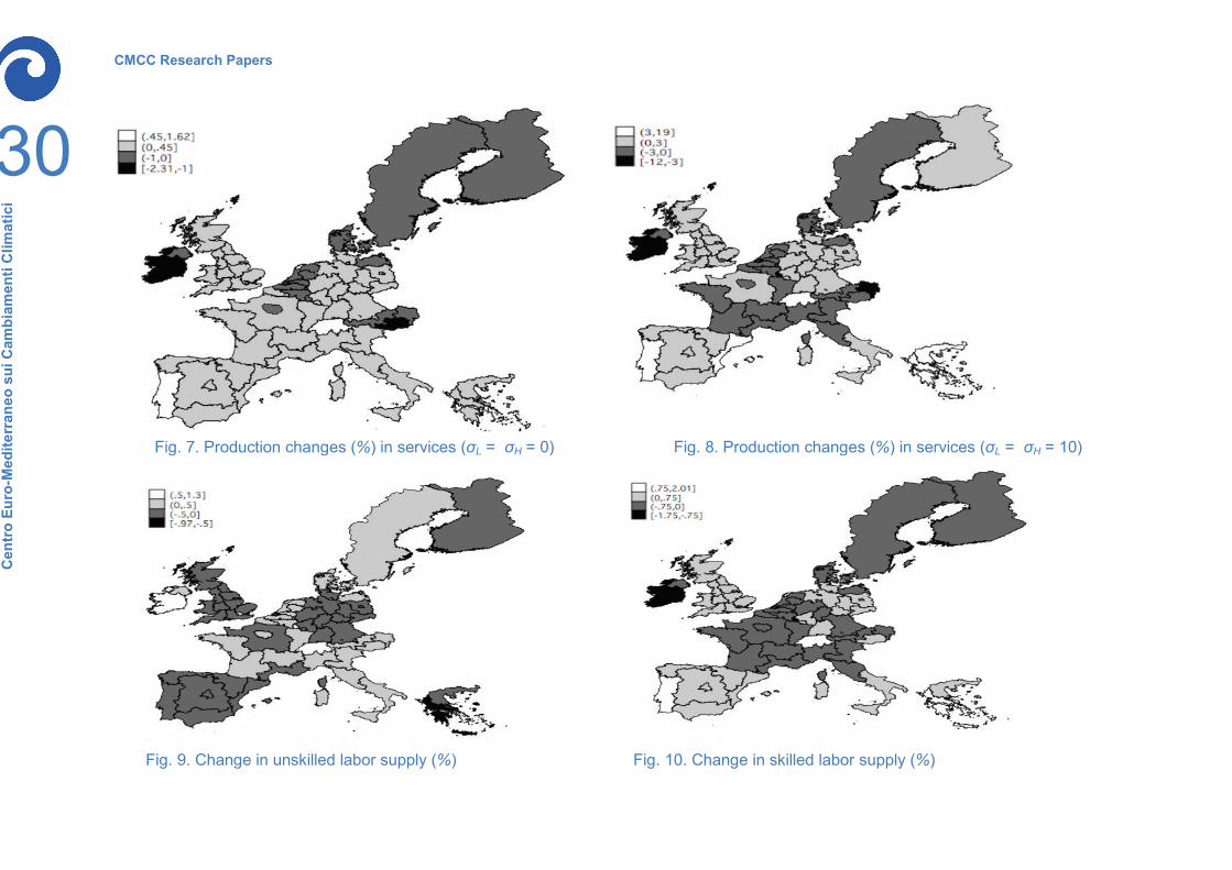
important at NUTS 1 level. Figures 3, 5 and 7 show these effects for the AGM, IND and

SERV sectors in the case of labor immobility.14At first glance, it appears that positive and

negative magnitudes are higher than those observed at macro-area level. In addition, the

changes are negative for all the NUTS 1 regions in the agricultural sector and both negative

and positive in manufactures and services. It is important to emphasize that the shock

strikes the same country at different strengths. For example, the South and Islands in Italy,

13 GAMS software and the CONOPT/NLP algorithm were used for simulations; there are 5197 equations

and 5197 variables. The numeraire is the utility price of a representative household in the ROW macro-area. 14 PRM is neglected, because its overall weight is almost insignificant in the EU15 economy and the relative

changes are always positive but quite small in all the scenarios for all NUTS 1 regions. The results for this sector are available upon request.


17

Cen

tro

Euro

-Med

iterr

aneo

sui

Cam

biam

enti

Clim

atic

i

Wales and the South-East in the UK, Centre East in France, and East in Germany are most

affected in the agricultural sector with respect to the rest of the country.

A sensitivity analysis is carried out to evaluate the impact of the labor mobility hypothesis

on trade policy results. As a result, the elasticity values of migration (σL and σH) are set at

10. Fig. 4, 6 and 8 show these effects for each of the 68 NUTS regions and for the AGM,

IND and SERV sectors in the case of labor mobility within the EU15 (the results are very

similar for the NUTS regions in the case of labor mobility within the EU27 and are not

reported). Agricultural production continues to decrease in all regions and the magnitudes

of the variations are also close to those observed in the labor immobility scenario. However,

huge amplification effects can be observed in manufactures and services; some regions

specialize strongly in the IND sector and others in the SERV sector. For example, in

manufactures, the Ile de France, Greater London, Ireland, East Austria, Brussels region,

Luxembourg and the Netherlands, except East, show an increase of about 5% or more,

while Greece, East, North West and Scotland in UK, Spain except North East, and

Brandenburg show a decrease of about 5% or more. Also in the labor mobility scenario, the

shock strikes the same country at different strengths, especially in the IND and SERV

sectors.

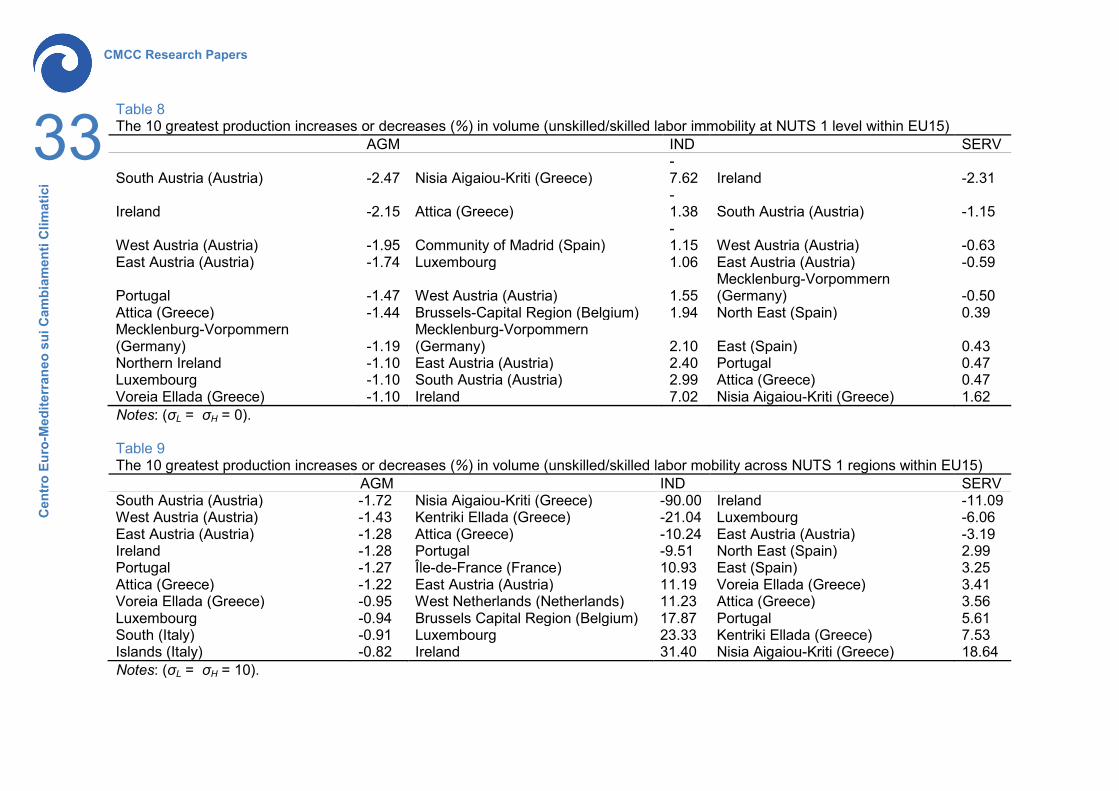
Table 8 focuses attention on the ten greatest (positive and negative) per cent changes in

the AGM, IND and SERV sectors in the case of labor immobility at NUTS 1 level. In

agriculture, Austrian regions, Ireland, Portugal, Attica (Greece) and Mecklenburg-

Vorpommern (Germany) display the greatest decreases, which range from 2.5% to 1.2%.

Using the MIRAGE-DREAM model and simulating complete liberalization (all tariffs are

removed and domestic support and export subsidies are cut by 50%), Jean and Laborde

(2004) find that regions in Ireland and Spain experience the greatest decreases in

agricultural value added in volume (more than 10% for Spanish regions and 20% for

Ireland). In our model, only the results for Ireland are consistent with the MIRAGE-DREAM

simulation. However, in the approach of Jean and Laborde (2004), unskilled and skilled

labor is imperfectly mobile within each European country of the EU25 and no sensitivity

analysis is carried out as regards the elasticity of migration. In addition, all sectors are

liberalized, so that the shock is stronger and more complex.

It is interesting to note the general equilibrium reallocation process between

manufactures and services in Table 8. For example, Nisia Aigaiou Kriti (Greece) and Attica


18

Cen

tro

Euro

-Med

iterr

aneo

sui

Cam

biam

enti

Clim

atic

i

(Greece) show both the greatest decrease in manufactures (7.62% and 1.38%,

respectively) and the greatest increase in services (1.62% and 0.47% respectively).

Conversely, Ireland and South Austria show the greatest increase in manufactures (7.02%

and 2.99%, respectively) and the greatest decrease in services (2.31% and 1.15%

respectively).

Table 9 lists the results of the ten greatest (positive and negative) per cent changes in

the AGM, IND and SERV sectors at NUTS 1 level in the case of labor mobility within the

EU15 (the results are very similar for NUTS regions in the case of labor mobility within the

EU27). Table 9 shows that the Austrian agricultural sector is the most badly stricken,

because all three of its regions (South Austria, West Austria, East Austria) rank in the first

three positions, although the changes are not great (between 1% and 2%). In line with the

results of the maps, the reallocation process between manufactures and services is

amplified and characterized by inverse patterns for some NUTS 1 regions. For example,

two Greek regions, Nisia Aigaiou-Kriti and Kentriki Ellada, have the highest positive values

for production change in services, 18.64% and 7.53%, respectively, and the greatest

negative values for production change in manufactures, -90.00% and -21.04%. Conversely,

Luxembourg and Ireland have the highest positive values for production change in

manufactures, 23.33% and 31.40%, respectively, and the greatest negative values for

production change in services, -6.06% and -11.09%. These results do not aim at being

realistic, because labor mobility is probably too high, but they are a guide to the importance

of the assumption about labor mobility.

Policy-makers are likely to be interested in labor reallocation across the NUTS 1 region

after agricultural liberalization. For this reason Fig. 9 and 10 show migration results for

unskilled and skilled labor levels, respectively, under the assumption of unskilled/skilled

labor mobility across NUTS 1 regions within the EU15.

It is interesting to note that the NUTS 1 regions displaying the highest sectoral

production reallocation also show the highest levels of unskilled/skilled labor reallocation.

Labor reallocation follows an inverse pattern in these NUTS 1 regions, according to their

sectoral specialization. For example, Ireland and Luxembourg absorb unskilled labor

because they increase production in the IND sector and decrease it in the SERV sector

after the trade shock, whereas Kentriki Ellada and Nisia Aigaiou-Kriti absorb skilled labor

because they decrease production in the IND sector and increase it in the SERV sector.

Basically, the results do not change with the integrated labor market within the EU27 for


19

Cen

tro

Euro

-Med

iterr

aneo

sui

Cam

biam

enti

Clim

atic

i

NUTS 1 regions. However, it can be noted that the REU experiences an unskilled/skilled

labor immigration, respectively 0.24% and 0.16%.

Lastly, welfare analysis is carried out at macro-area level. Welfare gains are measured

in equivalent variations (EV) $ million in the three labor market scenarios.

Under the assumption of unskilled/skilled labor immobility at NUTS 1 level within the

EU15, ROW gains about $5462 million. Gains are limited for the EU15 and REU, $157 and

$75 million, respectively.

Increasing labor mobility within the EU15 in the second scenario results in a slight

improvement in welfare. Indeed, the ROW gains $5616 million and the EU15 and REU,

$176 and $87 million, respectively. However, the gain for Europe as a whole continues to

be almost insignificant.

Assuming an integrated labor market within the EU27, the welfare increase for the ROW

macro-area is only $2 million ($5618). Interestingly, the EU15 loses and the REU wins in

the third scenario. Liberalization of agriculture determines a gain of about $408 million for

the REU and a loss by $160 million for the EU15. Nevertheless, gains and losses continue

to be almost insignificant for Europe.

It is worth noting that other studies produce much higher estimates of equivalent

variation. For example, with the GTAP model with perfect competition and constant returns

to scale in all sectors, Hertel and Keeney (2006) find that full liberalization of agriculture

(market access, domestic support and export subsidies) produce a $55 billion gain for the

world as a whole. With the MIRAGE model with imperfect competition in services and

manufactures, Bouet et al. (2005) implement probable Doha round agricultural

liberalization. They find a gain of $18 billion for the world as a whole. In addition in both

these two studies, baseline equilibrium in which trade liberalization is implemented

considers as achieved European enlargement and the other commitments which had taken

place by the end of 2004 (e.g., China's accession to the WTO). As a result, our model

probably overestimates further the welfare gain of tariff liberalization in agriculture, because

the world picture of tariff barriers is that of 2001. These different results may depend on the

NUTS regional level adopted to define the production structure.

Let us now examine the economic reasons for such results, especially our basic result,

production reallocation across sectors in each NUTS 1 region in the case of labor


20

Cen

tro

Euro

-Med

iterr

aneo

sui

Cam

biam

enti

Clim

atic

i

immobility. The stylized model is a useful tool to achieve this objective. There are two main

features concerning the results of trade policy simulation:

• different negative magnitudes of production change in the agricultural sector (AGM)

across NUTS 1 regions,

• different (positive and negative) magnitudes of production change across NUTS 1

regions in other sectors, manufactures (IND) and services (SERV).

Our model has four sectors and the stylised model only two. The result of this

simplification is that the different (positive and negative) magnitudes in the IND and SERV

sectors become different positive magnitudes in the skilled labor intensive sector. We

concentrate on Eq. (7), the technological condition, which gives the key parameter for

interpreting the results, i.e., the sectoral difference between the ratios of unskilled labor

intensity to skilled labor intensity. The following parameter is used in our model as proxy of

the key parameter in Eq. (7):

,,

, ,

,j ri r

i r j r

LLQ Q

ααα α

−

where i and j are sector indexes, r is the index of the NUTS 1 region, and αL and αQ are

parameters of the CES value added function for the unskilled and fictive factors. It is worth

recalling that fictive factor (Q) is a CES bundle of capital and skilled labor. Indeed, in our

model the valued added is specified through two-level nested technology (see Fig. 2).

To show how the parameter determines the per cent production changes, Table 10

matches the ten greatest per cent production decreases in volume at NUTS 1 level for the

AGM sector with the ten highest values of parameters α(agm/ind) and α(agm/serv). The

latter is the difference between the ratios of unskilled labor intensity to fictive factor intensity

in the AGM and SERV sectors, respectively. The former is the difference between the ratios

of unskilled labor intensity to fictive factor intensity, respectively, in AGM and IND.

Clearly, seven production changes match the corresponding key parameters for the

NUTS 1 regions in columns 2 and 4, and six production changes match the corresponding

key parameter for NUTS 1 regions in columns 6 and 8 (per cent production changes and

corresponding key parameters, which match each other, are shown in bold type).


21

Cen

tro

Euro

-Med

iterr

aneo

sui

Cam

biam

enti

Clim

atic

i

Therefore, in view of the production decrease in the agriculture sector for all the EU15

regions, the most affected regions are those in which there is a stronger sectoral difference

between AGM and other sectors in the relative use of unskilled and skilled factors. For

example, South Austria experiences the greatest decrease in AGM and uses more

intensively unskilled labor in AGM and skilled labor in IND and SERV with respect to the

other NUTS 1 regions.

A similar argument can be used to explain the different (positive and negative) per cent

production changes in IND and SERV, listed in Table 11.

So far, the reasons which cause different magnitudes in the three sectors have been

explained, but it is also important to understand the sign of the production change across

NUTS 1 regions. There is no doubt in the agricultural sector, because the sign is the same

for all NUTS 1 regions and this can therefore be interpreted as a result of the demand side

at macro-area level. In contrast, the sign changes in manufactures and services, and this

can be interpreted as one result of improved efficiency in the allocation of inputs, i.e., as a

result of the supply side at NUTS 1 level.

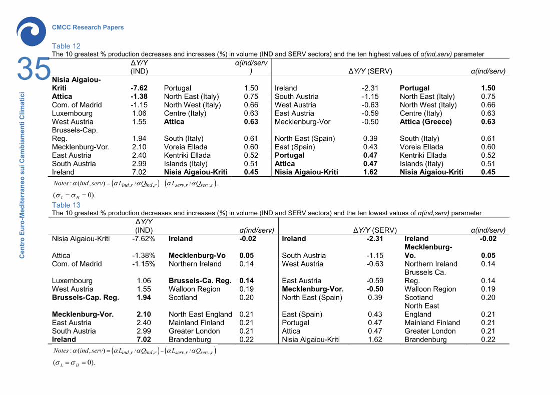
Tables 12 and 13 help us to understand the different signs in the IND and SERV sectors.

For example, the Greek regions, Nisia Aigaiou-Kriti and Attica, experience the greatest

decrease in IND and have a α(ind/serv) value included within the ten highest values. This

means that these regions use the unskilled labor in IND and the skilled labor in SERV more

intensively with respect to the other NUTS 1 regions. In contrast, Ireland experiences the

greatest increase in IND and has the lowest α(ind/serv) value. This means that Ireland uses

unskilled labor and skilled labor by similar intensities in both sectors with respect to the

other NUTS 1 regions.

A similar argument can be used for SERV. Tables 12 and 13 show Nisia Aigaiou-Kriti,

Attica and Portugal as the regions with the greatest increase in SERV, and they also have

α(ind/serv) values falling within the ten highest values. In contrast, Ireland experiences the

greatest decrease in SERV and has the lowest α(ind/serv) value.

Thus, the increases and decreases of the production change in IND and SERV are

characterized by inverse patterns at NUTS 1 level.

In Tables 12 and 13, only two out of ten or three out of ten production changes match

the corresponding key parameters. This means that further channels, in addition to the

sectoral difference between the ratios of unskilled labor intensity to skilled labor intensity


22

Cen

tro

Euro

-Med

iterr

aneo

sui

Cam

biam

enti

Clim

atic

i

may play a role in determining the sign in IND and SERV. However, the above-mentioned

channel, based on the α(ind/serv) parameter value, is probably very important because it

involves those NUTS 1 regions which show the highest increases and decreases in IND

and SERV, i.e., Ireland and Nisia Aigaiou-Kriti.

To summarize, trade policy strikes AGM and causes a production decrease in that

sector for all the NUTS 1 regions. The NUTS 1 regions, which use unskilled labor in AGM

and skilled labor in IND and SERV sectors more intensively with respect to the other NUTS

1 regions, are the most affected regions in AGM. The decrease in AGM production, in turn,

determines a production reallocation and reduces the labor demand for unskilled labor. As

a result, in general the unskilled factor loses (the wage goes down) and the skilled factor

wins (the wage goes up). However, in the NUTS 1 regions which use the unskilled labor in

IND and the skilled labor in SERV more intensively, IND production goes down and SERV

production goes up. In contrast, in the NUTS 1 regions, which use the unskilled and skilled

factors in IND and SERV sectors by similar intensities, the IND production goes up and the

SERV production goes down.

The relative variations are larger in absolute value in IND and SERV than those in AGM.

This depends on the fact that the agricultural sector also uses land and natural resources

and that these two factors are sector-specific. As a result, the overall mobility of the factors

and the relative production change are weaker in AGM.

The introduction of unskilled/skilled labor mobility within the EU15 and the EU27

continues to cause decreases in AGM for all regions but a larger production reallocation

between IND and SERV, as shown in Table 9. In agriculture, the relative changes are

stable, mainly because factors such as land and natural resources represent a constraint

and cannot move across regions. By contrast, strong amplification effects are observed in

IND and SERV for the NUTS 1 regions, which underwent large decreases or increases in

the case of unskilled/skilled labor immobility. These amplification effects occur because

workers can move toward regions where they receive a higher wage. This is also why the

Greek regions and Portugal exhibit a stronger skilled immigration (Fig. 11) while Ireland and

Luxembourg have a stronger unskilled immigration (Fig. 10).


23

Cen

tro

Euro

-Med

iterr

aneo

sui

Cam

biam

enti

Clim

atic

i

7. POLICY IMPLICATIONS AND CONCLUDING REMARKS

The contribution of this work merits the attention of policy-makers because it explores

trade policy effects for the EU15 at a disaggregated geographical level. We have shown

that the existence of various technologies across regions and sectors in the relative use of

unskilled and skilled labor factors generates different patterns of production changes. In

addition, although our trade model does not include heterogeneity in technologies, the

assumption of labor mobility can make a huge impact across sectors and regions. Thus, if

reduction in regional economic disparities is a political goal, the role played by technological

heterogeneity and labor mobility at regional level should be considered in policy

argumentations of current WTO negotiations.

The scenario of tariff agricultural liberalization causes a decrease in agricultural

production throughout the EU regions. In view of this general decrease, the reallocation

process involves especially services and manufactures. In the case of high labor mobility,

we observe strong amplification effects in these two sectors. These results are not intended

to be truly realistic, but they are suggested as a guide for policy-makers regarding the

importance of assumptions about labor mobility.

Some regions, especially in the Mediterranean countries, specialize in services because

they have a manufactures sector which still intensively uses unskilled labor. A typical

example is the textile sector in Mediterranean countries, which was greatly affected by

competition from emerging countries in these last years. Other regions, especially in

Northern Europe, specialize in manufactures because they use skilled labor in this sector

more intensively than other regions.

Some sectoral policy implications can be made from our picture of trade liberalization.

Agricultural production decreases in all regions but the magnitudes are not large, at most

about 2.5 per cent. The general equilibrium effects are more important in manufactures and

services, where perfect labor mobility across sectors determines larger variations,

depending on the fact that agriculture also uses land and natural resources and that these

two factors are sector-specific.

Lastly, it is worth noting that sectoral and geographical labor mobility implies a social

cost which is difficult to measure. As a consequence, policy-makers should strengthen

appropriate accompanying long-term policies, such as outplacement policies and aid to

geographical mobility, to compensate for this social cost in regions where the production


24

Cen

tro

Euro

-Med

iterr

aneo

sui

Cam

biam

enti

Clim

atic

i

and labor reallocation processes are stronger. Complementarily, model simulations also

predict that, after trade policy reforms, skilled labor wins (wages go up) and unskilled labor

loses (wages go down). For this reason, investment in education and training would also be

useful, to match this labor dynamics in agricultural trade liberalization.


25

Cen

tro

Euro

-Med

iterr

aneo

sui

Cam

biam

enti

Clim

atic

i

REFERENCES

Adams, D. (2005). Interpretation of results from CGE models such as GTAP. Journal of

Policy Modeling, 27(8), 941-959.

Anania, G., & Bureau, J.C. (2005). The Negotiations on agriculture in the Doha

development agenda round: current status and future prospects. European Review of

Agricultural Economics, 32(4), 539-550.

Bchir, H., Decreux, Y., Guerin, J.L., & Jean, S. (2002). MIRAGE, a computable general

equilibrium model for trade policy analysis. CEPII Working Paper No. 2002-17.

Bouet, A., Decreux, Y., Fontagne, L., Jean, S., & Laborde, D. (2004). A consistent, ad-

valorem equivalent measure of applied protection across the world: the MAcMap-HS6

database. CEPII Working Papers No. 2004-22.

Bouet, A., Bureau, J.C., Decreux, Y., & Jean, S. (2005). Multilateral Agricultural Trade

Liberalisation: The Contrasting Fortunes of Developing Countries in the Doha Round.

World Economy, 28(9), 1329–1354.

Dimaranan, B.V., & McDougall, R.A. (2005). Global trade, assistance, and production: The

GTAP 6 data base. Purdue University: Center for Global Trade Analysis.

Decreux, Y., & Valin, H. (2007). MIRAGE, updated version of the model for trade policy

analysis: Focus on agriculture and dynamics. CEPII Working Papers No. 2007-15.

Duffy, J., Papageorgiou, C., & Perez-Sebastian, F. (2004). Capital-Skill Complementarity?

Evidence from a panel of countries. The Review of Economics and Statistics, 86(1), 327-

344.

Eichengreen, B. (1993). Labor markets and European monetary unification. In P. Masson &

M. Taylor (Eds.), Policy issues in the operation of currency unions. Cambridge:

Cambridge University Press.

Hanslow, K., & Hinchy, M. (1996). The MEGABARE model: Interim documentation.

Canberra: ABARE (Australian Bureau of Agricultural and Resource Economics).

Hertel, T.W. (Ed.). (1997). Global trade analysis: Modeling and applications. Cambridge

and New York: Cambridge University Press.

Hertel, T. W., & Keeney, R. (2006). What's at stake: the relative importance of import

barriers, export subsidies and domestic support. In K. Anderson & W. Martin (Eds.),


26

Cen

tro

Euro

-Med

iterr

aneo

sui

Cam

biam

enti

Clim

atic

i

Agricultural trade reform and the Doha development agenda. Basingstoke: Palgrave

Macmillan.

Horridge, M., Madden, J., & Wittwer, G. (2005). The impact of the 2002-2003 drought on

Australia. Journal of Policy Modeling, 27(3), 285-308.

Jansson, T.G., Kuiper, M.H., & Adenäuer, M. (2009). Linking CAPRI and GTAP.

(http://www.seamless- ip.org/Reports/Report_39_D3.8.3.pdf).

Jean, S., & Laborde, D. (2004). The impact of multilateral liberalisation on European

regions: a CGE assessment. CEPII Working Paper No. 2004-20.

Laborde, D., & Valin, H. (June 2007). Exposure of EU regions to economic changes linked

to some potential EU trade agreements. Report for the Commission of the European

Union - Directorate-General for Trade.

Panagariya, A., & Duttagupta, R. (2001). The Gains from Preferential Trade Liberalization

in the CGE Models: Where do they come from. In S. Lahiri (Ed.), Regionalism and

globalization: Theory and practice (pp. 39-60). London and New York: Routledge.

Peter, M.W., Horridge, M., Meagher, G.A., Naqvi, F., & Parmenter, P.R. (1996). The

theoretical structure of MONASH-MRF. Centre of Policy Studies/IMPACT Centre

Working Papers op-85.

Yang, J., Huang, J., Li, N., Rozelle, S., & Martin, W. (2011). The impact of the Doha trade

proposals on farmers’ incomes in China. Journal of Policy Modeling, 33(3), 439-452.


27

Cen

tro

Euro

-Med

iterr

aneo

sui

Cam

biam

enti

Clim

atic

i

Fig. 1. Demand structure

Total demand in macro-area m for sector i

Domestic demand in macro-area m for sector i

Aggregate foreign demand in macro-area m for sector i

CES σARM

Foreign good from macro-area m’≠m for sector i

Foreign good from macro-area m’’≠m for sector i

CES σIMP


28

Cen

tro

Euro

-Med

iterr

aneo

sui

Cam

biam

enti

Clim

atic

i

Fig. 2. Supply structure

Production in sector i and region r

Aggregate intermediate input in sector i and region r

Value added in sector i and region r

Fictive factor in sector i and

region r

Unskilled labour in

sector i and region r

Natural resources in sector i and

region r

Capital in sector i and

region r

Intermediate input in sector i

and region r from sector ..

Land in sector i and region r


and region r from sector I

Skilled labour in sector i and

region r


and region r from sector 1

Leontief

CES σVA

CES σINI

CES σQ


29

Cen

tro

Euro

-Med

iterr

aneo

sui

Cam

biam

enti

Clim

atic

i

Fig. 3. Production changes in agriculture (σL = σH = 0) Fig. 4. Production changes (%) in agriculture (σL = σH = 10)

Fig. 5. Production changes (%) in manufactures (σL = σH = 0) Fig. 6. Production changes(%) in manufactures (σL = σH = 10)


30

Cen

tro

Euro

-Med

iterr

aneo

sui

Cam

biam

enti

Clim

atic

i

Fig. 7. Production changes (%) in services (σL = σH = 0) Fig. 8. Production changes (%) in services (σL = σH = 10)

Fig. 9. Change in unskilled labor supply (%) Fig. 10. Change in skilled labor supply (%)


31

Cen

tro

Euro

-Med

iterr

aneo

sui

Cam

biam

enti

Clim

atic

i

Table 1 Sectoral aggregation (4 sectors) Sectors AGM Agriculture and minerals PRM Primary energy sources IND Manufactures SERV Services

Table 2 First geographical level of aggregation (3 macro-areas) Macro-areas EU15 Austria, Belgium, Denmark, Finland, France, Germany, Greece,

Ireland, Italy, Luxembourg, Netherlands, Portugal, Spain, Sweden, United Kingdom

REU Bulgaria, Cyprus, Czech Republic, Estonia, Hungary, Latvia, Lithuania, Malta, Poland, Romania, Slovakia, Slovenia

ROW Rest of the world Table 3 Second geographical level of aggregation (68 NUTS 1 regions) NUTS 1 regions Austria East Austria, South Austria, West Austria Belgium Brussels Capital Region, Flemish Region, Walloon Region Denmark Denmark Finland Mainland Finland, Ǻland France Île-de-France, Parisian basin, Nord-Pas-de-Calais, East, West,

South West, Centre East, Mediterranean Germany Baden-Wüttenberg, Bavaria, Berlin, Brandenburg, Bremen,

Hamburg, Hessen, Mecklenburg-Vorpommern, Lower Saxony, North Rhine-Westphalia, Rhineland-Palatinate, Saarland, Saxony, Saxony-Anhalt, Schleswig-Holstein, Thuringia

Greece Voreia Ellada, Kentriki Ellada, Attica, Nisia Aigaiou-Kriti Ireland Ireland Italy North West, North East, Centre, South, Islands Luxembourg Luxembourg Netherlands North Netherlands, East Netherlands, West Netherlands, South

Netherlands Portugal Portugal Spain North West, North East, Community of Madrid, Centre, East,

South Sweden Sweden United Kingdom

North East England, North West England, Yorkshire and the Humber, East Midlands, West Midlands, East of England, Greater London, South-East England, South-West England, Wales, Scotland, Northern Ireland


32

Cen

tro

Euro

-Med

iterr

aneo

sui

Cam

biam

enti

Clim

atic

i

Table 4 Ad valorem equivalent tariffs (%)

ROW EU15 REU AGM ROW 14.73 5.27 5.65 AGM EU15 10.70 10.37 AGM REU 12.69 4.95 6.11 PRM ROW 1.64 0.20 PRM EU15 0.01 0.00 PRM REU 0.30 0.88 IND ROW 5.10 2.83 6.85 IND EU15 6.10 3.38 IND REU 6.97 0.76 3.97 Notes: Column 2 shows macro-area where good is produced and row 1 the macro-area applying tariffs. Table 5 Production changes (%) in volume (unskilled/skilled labor immobility at NUTS 1 level within EU15)

ROW EU15 REU AGM 0.32 -0.93 -0.58 PRM -0.10 0.07 0.01 IND 0.01 0.00 0.05 SERV -0.02 0.05 0.04 Notes: (σL = σH = 0).

Table 6 Production changes (%) in volume (unskilled/skilled labor mobility across NUTS 1 regions within EU15) ROW EU15 REU AGM 0.32 -0.76 -0.57 PRM -0.07 0.16 0.05 IND 0.01 0.13 0.05 SERV -0.02 0.08 0.04 Notes: (σL = σH = 10). Table 7 Production changes (%) in volume (unskilled/skilled labor mobility within EU27) ROW EU15 REU AGM 0.32 -0.76 -0.46 PRM -0.06 0.16 0.15 IND 0.01 0.13 0.17 SERV -0.02 0.08 0.14 Notes: (σL = σH = 10 in integrated EU27 labor market).


33

Cen

tro

Euro

-Med

iterr

aneo

sui

Cam

biam

enti

Clim

atic

i

Table 8 The 10 greatest production increases or decreases (%) in volume (unskilled/skilled labor immobility at NUTS 1 level within EU15)

AGM IND SERV

South Austria (Austria) -2.47 Nisia Aigaiou-Kriti (Greece) -7.62 Ireland -2.31

Ireland -2.15 Attica (Greece) -1.38 South Austria (Austria) -1.15

West Austria (Austria) -1.95 Community of Madrid (Spain) -1.15 West Austria (Austria) -0.63

East Austria (Austria) -1.74 Luxembourg 1.06 East Austria (Austria) -0.59

Portugal -1.47 West Austria (Austria) 1.55 Mecklenburg-Vorpommern (Germany) -0.50

Attica (Greece) -1.44 Brussels-Capital Region (Belgium) 1.94 North East (Spain) 0.39 Mecklenburg-Vorpommern (Germany) -1.19

Mecklenburg-Vorpommern (Germany) 2.10 East (Spain) 0.43

Northern Ireland -1.10 East Austria (Austria) 2.40 Portugal 0.47 Luxembourg -1.10 South Austria (Austria) 2.99 Attica (Greece) 0.47 Voreia Ellada (Greece) -1.10 Ireland 7.02 Nisia Aigaiou-Kriti (Greece) 1.62

Notes: (σL = σH = 0). Table 9 The 10 greatest production increases or decreases (%) in volume (unskilled/skilled labor mobility across NUTS 1 regions within EU15)

AGM IND SERV South Austria (Austria) -1.72 Nisia Aigaiou-Kriti (Greece) -90.00 Ireland -11.09 West Austria (Austria) -1.43 Kentriki Ellada (Greece) -21.04 Luxembourg -6.06 East Austria (Austria) -1.28 Attica (Greece) -10.24 East Austria (Austria) -3.19 Ireland -1.28 Portugal -9.51 North East (Spain) 2.99 Portugal -1.27 Île-de-France (France) 10.93 East (Spain) 3.25 Attica (Greece) -1.22 East Austria (Austria) 11.19 Voreia Ellada (Greece) 3.41 Voreia Ellada (Greece) -0.95 West Netherlands (Netherlands) 11.23 Attica (Greece) 3.56 Luxembourg -0.94 Brussels Capital Region (Belgium) 17.87 Portugal 5.61 South (Italy) -0.91 Luxembourg 23.33 Kentriki Ellada (Greece) 7.53 Islands (Italy) -0.82 Ireland 31.40 Nisia Aigaiou-Kriti (Greece) 18.64

Notes: (σL = σH = 10).


34

Cen

tro

Euro

-Med

iterr

aneo

sui

Cam

biam

enti

Clim

atic

i

Table 10 The 10 greatest production decreases (%) in volume (AGM sector) and ten highest values of α(agm,ind) and α(agm,serv) parameters

ΔY/Y

(AGM) α(agm/ind) ΔY/Y (AGM) α(agm/serv) South Austria -2.47 South Austria 4.79 South Austria -2.47 South Austria 5.05 Ireland -2.15 West Austria 3.50 Ireland -2.15 Portugal 4.41 West Austria -1.95 Kentriki Ellada 3.15 West Austria -1.95 West Austria 3.79 East Austria -1.74 Nisia Aigaiou-Kriti 2.96 East Austria -1.74 Kentriki Ellada 3.67 Portugal -1.47 Portugal 2.91 Portugal -1.47 Nisia Aigaiou-Kriti 3.41 Attica -1.44 East Austria 2.73 Attica -1.44 Voreia Ellada 3.25 Mecklenburg-Vor. -1.19 Voreia Ellada 2.65 Mecklenburg-Vor. -1.19 East Austria 2.98 Northern Ireland -1.10 Attica 2.09 Northern Ireland -1.10 Attica 2.72 Luxembourg -1.10 Ireland 1.58 Luxembourg -1.10 South (Italy) 2.02 Voreia Ellada -1.10 South (Italy) 1.41 Voreia Ellada -1.10 Islands (Italy) 1.63

( ) ( ) ( ) ( ), , , , , , , ,/ / , / / . : ( , ) ( , )

( 0).L H

agm r agm r ind r ind r agm r agm r serv r serv rNotes agm ind L Q L Q agm serv L Q L Qα α α α α α α α α α

σ σ

− −= =

= =

Table 11 The 10 greatest production decreases and increases (%) in volume (IND and SERV sectors) and the ten highest values of α(agm,ind) and α(agm,serv) parameters

ΔY/Y (IND) α(agm/ind) ΔY/Y (SERV) α(agm/serv)

Nisia Aigaiou-Kriti -7.62 South Austria 4.79 Ireland -2.31 South Austria 5.05 Attica -1.38 West Austria 3.50 South Austria -1.15 Portugal 4.41 Community of Madrid -1.15 Kentriki Ellada 3.15 West Austria -0.63 West Austria 3.79 Luxembourg 1.06 Nisia Aigaiou-Kriti 2.96 East Austria -0.59 Kentriki Ellada 3.67

West Austria 1.55 Portugal 2.91 Mecklenburg-Vor. -0.50 Nisia Aiga. -Kriti 3.41

Brussels-Cap. Region 1.94 East Austria 2.73 North East (Spain) 0.39 Voreia Ellada 3.25 Mecklenburg-Vor. 2.10 Voreia Ellada 2.65 East (Spain) 0.43 East Austria 2.98 East Austria 2.40 Attica 2.09 Portugal 0.47 Attica 2.72 South Austria 2.99 Ireland 1.58 Attica 0.47 South (Italy) 2.02 Ireland 7.02 South (Italy) 1.41 Nisia Aigaiou-Kriti 1.62 Islands (Italy) 1.63

( ) ( ) ( ) ( ), , , , , , , ,/ / , / / .: ( , ) ( , )

( 0).L H

agm r agm r ind r ind r agm r agm r serv r serv rNotes agm ind L Q L Q agm serv L Q L Qα α α α α α α α α α

σ σ

− −= =

= =


35

Cen

tro

Euro

-Med

iterr

aneo

sui

Cam

biam

enti

Clim

atic

i

Table 12 The 10 greatest % production decreases and increases (%) in volume (IND and SERV sectors) and the ten highest values of α(ind,serv) parameter

ΔY/Y (IND)

α(ind/serv) ΔY/Y (SERV) α(ind/serv)

Nisia Aigaiou-Kriti -7.62 Portugal 1.50 Ireland -2.31 Portugal 1.50 Attica -1.38 North East (Italy) 0.75 South Austria -1.15 North East (Italy) 0.75 Com. of Madrid -1.15 North West (Italy) 0.66 West Austria -0.63 North West (Italy) 0.66 Luxembourg 1.06 Centre (Italy) 0.63 East Austria -0.59 Centre (Italy) 0.63 West Austria 1.55 Attica 0.63 Mecklenburg-Vor -0.50 Attica (Greece) 0.63 Brussels-Cap. Reg. 1.94 South (Italy) 0.61 North East (Spain) 0.39 South (Italy) 0.61 Mecklenburg-Vor. 2.10 Voreia Ellada 0.60 East (Spain) 0.43 Voreia Ellada 0.60 East Austria 2.40 Kentriki Ellada 0.52 Portugal 0.47 Kentriki Ellada 0.52 South Austria 2.99 Islands (Italy) 0.51 Attica 0.47 Islands (Italy) 0.51 Ireland 7.02 Nisia Aigaiou-Kriti 0.45 Nisia Aigaiou-Kriti 1.62 Nisia Aigaiou-Kriti 0.45

( ) ( ), , , ,/ / .: ( , )

( 0).L H

ind r ind r serv r serv rNotes ind serv L Q L Qα α α α α

σ σ

−=

= =

Table 13 The 10 greatest % production decreases and increases (%) in volume (IND and SERV sectors) and the ten lowest values of α(ind,serv) parameter

ΔY/Y (IND) α(ind/serv) ΔY/Y (SERV) α(ind/serv)

Nisia Aigaiou-Kriti -7.62% Ireland -0.02 Ireland -2.31 Ireland -0.02

Attica -1.38% Mecklenburg-Vo 0.05 South Austria -1.15 Mecklenburg-Vo. 0.05

Com. of Madrid -1.15% Northern Ireland 0.14 West Austria -0.63 Northern Ireland 0.14

Luxembourg 1.06 Brussels-Ca. Reg. 0.14 East Austria -0.59 Brussels Ca. Reg. 0.14

West Austria 1.55 Walloon Region 0.19 Mecklenburg-Vor. -0.50 Walloon Region 0.19 Brussels-Cap. Reg. 1.94 Scotland 0.20 North East (Spain) 0.39 Scotland 0.20

Mecklenburg-Vor. 2.10 North East England 0.21 East (Spain) 0.43 North East England 0.21

East Austria 2.40 Mainland Finland 0.21 Portugal 0.47 Mainland Finland 0.21 South Austria 2.99 Greater London 0.21 Attica 0.47 Greater London 0.21 Ireland 7.02 Brandenburg 0.22 Nisia Aigaiou-Kriti 1.62 Brandenburg 0.22

( ) ( ), , , ,/ /: ( , )

( 0).L H

ind r ind r serv r serv rNotes ind serv L Q L Qα α α α α

σ σ

−=

= =

36

Cen

tro

Eur

o-M

edite

rran

eosu

iCam

biam

enti

Clim

atic

i


c© Centro Euro-Mediterraneo sui Cambiamenti Climatici 2014

Visit www.cmcc.it for information on our activities and publications.

The Euro-Mediteranean Centre on Climate Change is a Ltd Company with its registered office andadministration in Lecce and local units in Bologna, Venice, Capua, Sassari, Viterbo, Benevento and Milan.The society doesn’t pursue profitable ends and aims to realize and manage the Centre, its promotion, andresearch coordination and different scientific and applied activities in the field of climate change study.

Date post:	02-Apr-2018
Category:	Documents
Upload:	dinhanh
View:	221 times
Download:	4 times

World tariff liberalization in agriculture: an … tariff liberalization in agriculture: an...

Documents