Write-limited sorts and joins for persistent memory

Stratis D. ViglasSchool of Informatics

University of Edinburgh, UK

sviglas@inf.ed.ac.uk

ABSTRACTTo mitigate the impact of the widening gap between the mem-ory needs of CPUs and what standard memory technology can de-liver, system architects have introduced a new class of memorytechnology termed persistent memory. Persistent memory is byte-addressable, but exhibits asymmetric I/O: writes are typically oneorder of magnitude more expensive than reads. Byte addressabil-ity combined with I/O asymmetry render the performance profileof persistent memory unique. Thus, it becomes imperative to findnew ways to seamlessly incorporate it into database systems. Wedo so in the context of query processing. We focus on the funda-mental operations of sort and join processing. We introduce thenotion of write-limited algorithms that effectively minimize the I/Ocost. We give a high-level API that enables the system to dynam-ically optimize the workflow of the algorithms; or, alternatively,allows the developer to tune the write profile of the algorithms. Wepresent four different techniques to incorporate persistent memoryinto the database processing stack in light of this API. We have im-plemented and extensively evaluated all our proposals. Our resultsshow that the algorithms deliver on their promise of I/O-minimalityand tunable performance. We showcase the merits and deficienciesof each implementation technique, thus taking a solid first step to-wards incorporating persistent memory into query processing.

1. INTRODUCTIONPersistent memory is a new class of memory technology that has

the potential to deliver on the promise of a universal storage de-vice. That is, a storage device with capacity comparable to that ofhard disk drives; and access latency comparable to that of randomaccess memory (DRAM). Database systems, as one of the primeconsumers of this technology, must be prepared for this transitionif they are to sustain the high performance users have come to ex-pect. Therefore, database developers need to optimize query pro-cessing operations for persistent memory. Likewise, it is necessaryto introduce abstractions that will incorporate this technology in aninformed way into the processing stack of database systems. Asthis technology rapidly evolves, the abstractions should be resilientto future trends and be system- and user-tunable.

This work is licensed under the Creative Commons Attribution-NonCommercial-NoDerivs 3.0 Unported License. To view a copy of this li-cense, visit http://creativecommons.org/licenses/by-nc-nd/3.0/. Obtain per-mission prior to any use beyond those covered by the license. Contactcopyright holder by emailing info@vldb.org. Articles from this volumewere invited to present their results at the 40th International Conference onVery Large Data Bases, September 1st - 5th 2014, Hangzhou, China.Proceedings of the VLDB Endowment, Vol. 7, No. 5Copyright 2014 VLDB Endowment 2150-8097/14/01.

high-performance diskmain memory

21 23 25 27 29 211 213 215 217 219 221 223

L1 cache LL cache DRAM persistentmemory flash HDD

Figure 1: Typical access latency in processor cycles on a 4GHzprocessor (figure adapted from [22])

The need for persistent memory is practical. The increase of thenumber of cores per CPU dictates that the memory system primarilyscale in terms of capacity as it must cater for the working sets of allconcurrently executing processes across all cores; and secondarilyin terms of data transfer rate to keep up with the increased demand.The growth rate of the number of cores per CPU is higher than thegrowth rate of DRAM capacity, and that gap only widens [13]. Sys-tem architects have thus worked on memory technologies that de-liver performance comparable to DRAM but at much higher capaci-ties. Persistent memory (also referred to as non-volatile memory) isan umbrella term encompassing all such efforts (e.g., phase-changememory). In terms of access latency, persistent memory sits be-tween DRAM and block-based flash memory, as shown in Figure 1.Thus, persistent memory is a new level in the memory hierarchy,the design space of which is only now starting to be explored.

There are various technical reasons why persistent memory war-rants a study of its own. Foremost, persistent memory is byte-addressable. This is in stark contrast to block-addressable flashmemory. The block-oriented techniques that have been proposedfor leveraging flash memory are inapplicable (see, e.g., [17] for areview of such techniques). Then, persistent memory latencies arecloser to DRAM than flash memory. The read latency is only 2-4times slower than DRAM compared to the 32 times slower-than-DRAM latency of flash [22]. At the same time persistent memoryexhibits the write performance problems of flash memory: writesare more than one order of magnitude slower than DRAM, and thusmore expensive than reads [17]. Persistent memory cells also havelimited endurance, which dictates wear-leveling data moves acrossthe device to increase its lifetime, thereby further amplifying writedegradation. Thus, persistent memory should be treated neitheras byte-addressable DRAM nor as block-addressable flash memory;while it exhibits some of the merits and deficiencies of both.

The properties of persistent memory require revisiting existingwork and optimizing it for the new medium. It is imperative thatnew algorithms and techniques are developed if database systemsare to make the best possible use of this new technology; other-wise, they are doomed to the suboptimal performance that stemsfrom false assumptions. Our key objective is to optimize writes asthey manifest the performance problems due to both byte address-ability and write/read asymmetry. The byte addressability of persis-tent memory renders flash-centric, block-based techniques inappli-

413

cable; while main-memory techniques do not differentiate betweenwrite and read cost asymmetry. To address these issues we willpresent a host of techniques that we term write-limited, which aimto seamlessly incorporate persistent memory in the data manage-ment stack. We will focus on key processing operations, namelysorts and joins, that are necessary for high-performing query eval-uation. At the same time, we will present abstractions to introducepersistent memory into the system in ways that allow both the sys-tem and the developer to optimize performance.Contributions and organization. Our contributions and the struc-ture of the rest of this paper are as follows:• We devise sort and join algorithms that minimize I/O by trad-

ing expensive writes for cheaper reads (Section 2). Addition-ally, the algorithms allow the developer to tune their writeintensity for a small hit on performance.• We provide ways to implement these algorithms by propos-

ing a flexible API (Section 3.1). Our API records a blueprintof each algorithm’s computation and enables the system todynamically decide whether to trade writes for reads.• We present four alternative implementations to incorporate

persistent memory into the processing stack of a query pro-cessor (Section 3.2). The implementations conform to ourproposed API and adhere to a common abstraction. Theyhave been selected to showcase the duality of persistent mem-ory as a non-volatile storage medium with performance char-acteristics close to volatile memory.• We experimentally evaluate our algorithms and implementa-

tion alternatives in a variety of scenarios (Section 4). Ourresults show that it is indeed possible to have efficient sortand join algorithms that minimize the number of write oper-ations without compromising performance. Our results alsoquantify the impact of implementations on performance andpoint out the subtleties in incorporating persistent memory inthe data processing stack.

Finally, we present related work in Section 5 and conclude andidentify future work directions in Section 6.

2. ALGORITHMIC FRAMEWORKOur algorithms are based on trading writes for reads. There are

two classes of algorithms. In the first class the computation is splitinto two parts: (a) a write-incurring part; and (b) a write-limitedpart that performs minimal writes. Such algorithms allocate differ-ent portions of the input to the write-incurring and the write-limitedparts. The portion allocation can be either informed, through a costmodel that minimizes the total I/O cost; or user-driven, allowing theuser to set the write intensity of the algorithm. The second class ofalgorithms is based on lazy processing. Lazy algorithms keep trackof the penalty being paid by performing extra reads and the man-ifested savings. Once the penalty plus the cost of generating anintermediate result exceed the savings, the algorithms generate theintermediate result and revert to being lazy.

Throughout the presentation we assume that persistent memoryI/O takes place in units we term buffers. Though persistent memoryis byte-addressable, most systems will perform I/O in larger chunksto amortize costs. These chunks are not as big as standard databasepages (i.e., four or eight kilobytes) but are equal to some small mul-tiple of the word size. Typically, they will be equal to the cachelinesize (i.e., 64 or 128 bytes). Reading a chunk costs r cost units,while writing it costs w units; λ = w/r is the write/read cost ratio;λ > 1. We will also be doing away with ceiling and floor functions.Doing so, though not strictly correct mathematically, simplifies theanalysis: as the buffer size is small, the error margin in omitting

floor and ceiling functions is quite small too. We will start withsorting before expanding to join processing.

2.1 Sorting algorithms

2.1.1 Segment sortThe starting point is traditional external mergesort. External

mergesort proceeds by splitting the input into chunks that fit inmain memory, using an in-memory algorithm to sort the values inthe chunk, and then writing the sorted chunks to disk as a run. Runsare then merged in passes to produce the sorted output. The numberof merging passes is dictated by the amount of available memory.Assume there are M buffers available for sorting; for a relation T of|T | buffers, the size of each run will be M for a total number of |T |/M

runs. During the merging phase we can have at most M runs open;the number of merging passes will be equal to logM |T |. In eachmerging pass the input will be fully read and written; the cost ofeach pass will be r+w = r(1+λ ). The total cost of the algorithmis then |T |r(1+λ )+ logM |T |r(1+λ )= |T |r(1+λ )(logM |T |+1).

Consider now a generalization of selection sort which, at a costof extra reads, writes each element of the input once at its final lo-cation. For a memory budget of M buffers, this algorithm worksin multiple passes, generating a run during each pass. During thefirst pass it scans the input to identify the M minimum values. Thiscan be achieved by maintaining a heap of values, e.g., a max-heapwhen sorting in ascending order. For each value t ∈ T either: (a) tis less than the current maximum, so the value belongs to the cur-rent run; or (b) t is greater than or equal to the maximum, so thevalue belongs to the next run. This is reminiscent of run generationduring external mergesort with replacement selection. When theinput is exhausted the contents of the heap are sorted and written.When writing we keep track of the maximum element and its po-sition in the input (which is recorded whenever the maximum heapelement is updated). During the next scan two more conditionsare added for an element to be inserted into the heap: (a) its valuemust be greater than or equal to the maximum of the previous run;and (b) its position must be greater than the position of the maxi-mum element of the previous run. These conditions ensure there isno overlap between runs. All subsequent iterations check all fourconditions before adding an element to a run. For an input T thealgorithm will perform |T ||T |/M read passes over the input and |T |writes for a total cost of |T ||T |/Mr+ |T |w = r|T |(|T |/M+λ ).

Let us now combine the two algorithms into a new one, whichwe term segment sort. Let x∈ (0,1) be the fraction of the input thatwill be sorted using external mergesort; the remaining (1− x)% ofthe input will be turned into a longer run using selection sort. Wecall x the write intensity of the algorithm. The input is split intotwo segments, each processed by a different algorithm. Runs willbe merged using the standard merging phase of external merge-sort. We assume external mergesort will execute first though thisrestriction can be easily lifted. Let us further assume that we willmaterialize the output (though it may well not need be materializedif it is to be pipelined to subsequent operators). The total cost Sh ofthis algorithm will be dependent on x and will be given by Eq. 1.

Sh(x) =x|T |r(1+λ )+(1− x)|T |r ((1− x)|T |/M+λ )

+ |T |r(1+λ ) logM (x|T |/2M+1)(1)

The first factor of the sum is the cost of generating the runs throughreplacement selection in external mergesort; the second factor is thecost of generating the longer run through selection sort; the thirdfactor is the cost of merging all runs assuming that external merge-sort generates runs that are, on average, twice the amount of mainmemory. To simplify the analysis assume that logM (x|T |/2M+1)≈

414

logM (x|T |/2M), which is true for large values of |T |. After factoringcommon terms the cost of the algorithm is given by Eq. 2.

Sh(x) =|T |r(x+λ )+ |T |2r/M(x2−2x+1)+ |T |r(λ +1) logM (x|T |/2M)

(2)

Our aim is to minimize Sh(x); that is, Shx(x) = 0, or: |T |r+(2x−

2)|T |2r/M +(λ+1)lnM

1x |T |r = 0; Factoring out |T |r and since |T |r 6= 0

we need to solve Eq. 3 for x.

2(x−1)|T |M

+(λ +1)

lnM1x= 0 (3)

The resulting quadratic equation has the two solutions given byEq. 4. The second solution is clearly negative, so the plus-signsolution is the only admissible value for x.

x =− lnM|T |±

√lnM (lnM|T |2 +2|T |M lnM−λM2)

M lnM(4)

Sanity checking. Apart from the second derivative Shxx(x) being

positive making this a minimum value, a few other constraints musthold. Firstly, the square root in Eq. 4 must be positive, which, afterfactorization, results in λ <

lnM|T |(|T |+2M)M2 . Assume that |T |= βM

for some value β > 1. The inequality is rewritten as λ < β (β +2) lnM which holds for all realistic values of λ . Secondly, x∈ (0,1)must hold. For x > 0 to hold the numerator must be positive, so:

lnM|T |<√

lnM(lnM|T |2 +2|T |M lnM−λM2

)must hold. Both sides are positive so we square them:

ln2 M|T |< lnM(

lnM|T |2 +2|T |M lnM−λM2)

and, after simplification, the inequality holds if λ <2lnM|T |

M . As-suming again that |T |= βM we obtain that λ < 2β lnM must hold.This is again true for most realistic values of λ , though it is a tighterbound than before. Finally x < 1 must hold, which means that:√

lnM(lnM|T |2 +2|T |M lnM−λM2

)< lnM(M+ |T |)

must be true. After squaring both sides and simplifying the resultis that λ >− lnM must hold, which is always true. From the abovewe conclude that for the algorithm to be applicable λ < 2|T |/M lnMmust hold (obtained by substituting β with |T |/M).Choosing segment algorithms and generalizing. We have sofar assumed that the first segment of the file is sorted using exter-nal mergesort and the second using selection sort; this may well beinversed. In terms of the chosen percentage it is likely that x willbe greater than 0.5; otherwise the quadratic contribution of the se-lection sort scans will quickly surpass the savings due to avoidingwrites. One can devise a second version of segment sort that doesnot minimize response time; rather, it does not surpass a specifiednumber of writes. If we set x to zero then external mergesort is notexecuted at all and the algorithm performs the minimum number ofwrites: as many as there are buffers in T . We can relax this mini-mality requirement and allow a variable number of extra writes bymanually setting x. Roughly, each percentile of the input allocatedto external mergesort will result in corresponding extra writes: itwill need to be sorted using external mergesort, while the results ofthe two sorted segments will need to be merged for the final output.

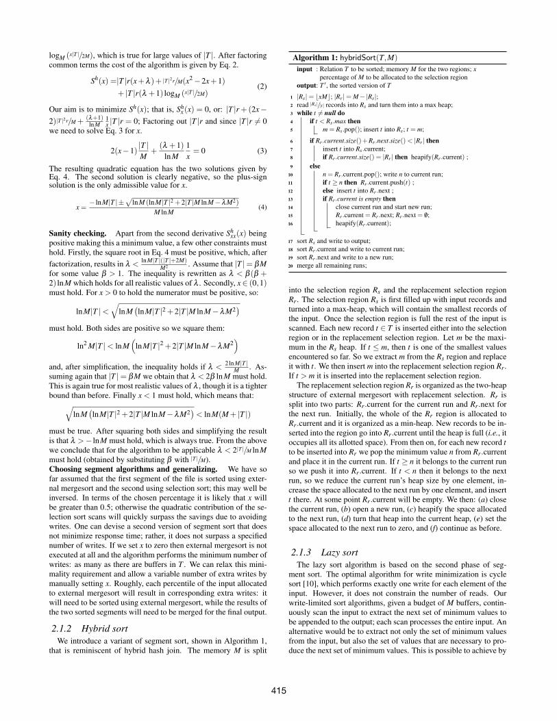
2.1.2 Hybrid sortWe introduce a variant of segment sort, shown in Algorithm 1,

that is reminiscent of hybrid hash join. The memory M is split

Algorithm 1: hybridSort(T,M)

input : Relation T to be sorted; memory M for the two regions; xpercentage of M to be allocated to the selection region

output: T ′, the sorted version of T

1 |Rs|= bxMc; |Rr |= M−|Rs|;2 read |Rs |/|t| records into Rs and turn them into a max heap;3 while t 6= null do4 if t < Rs.max then5 m = Rs.pop(); insert t into Rs; t = m;

6 if Rr .current.size()+Rr .next.size()< |Rr | then7 insert t into Rs.current;8 if Rr .current.size() = |Rr | then heapify(Rr .current) ;9 else

10 n = Rr .current.pop(); write n to current run;11 if t ≥ n then Rr .current.push(t) ;12 else insert t into Rr .next ;13 if Rr .current is empty then14 close current run and start new run;15 Rr .current = Rr .next; Rr .next = /0;16 heapify(Rr .current);

17 sort Rs and write to output;18 sort Rr .current and write to current run;19 sort Rr .next and write to a new run;20 merge all remaining runs;

into the selection region Rs and the replacement selection regionRr. The selection region Rs is first filled up with input records andturned into a max-heap, which will contain the smallest records ofthe input. Once the selection region is full the rest of the input isscanned. Each new record t ∈ T is inserted either into the selectionregion or in the replacement selection region. Let m be the maxi-mum in the Rs heap. If t ≤ m, then t is one of the smallest valuesencountered so far. So we extract m from the Rs region and replaceit with t. We then insert m into the replacement selection region Rr.If t > m it is inserted into the replacement selection region.

The replacement selection region Rr is organized as the two-heapstructure of external mergesort with replacement selection. Rr issplit into two parts: Rr.current for the current run and Rr.next forthe next run. Initially, the whole of the Rr region is allocated toRr.current and it is organized as a min-heap. New records to be in-serted into the region go into Rr.current until the heap is full (i.e., itoccupies all its allotted space). From then on, for each new record tto be inserted into Rr we pop the minimum value n from Rr.currentand place it in the current run. If t ≥ n it belongs to the current runso we push it into Rr.current. If t < n then it belongs to the nextrun, so we reduce the current run’s heap size by one element, in-crease the space allocated to the next run by one element, and insertt there. At some point Rr.current will be empty. We then: (a) closethe current run, (b) open a new run, (c) heapify the space allocatedto the next run, (d) turn that heap into the current heap, (e) set thespace allocated to the next run to zero, and (f) continue as before.

2.1.3 Lazy sortThe lazy sort algorithm is based on the second phase of seg-

ment sort. The optimal algorithm for write minimization is cyclesort [10], which performs exactly one write for each element of theinput. However, it does not constrain the number of reads. Ourwrite-limited sort algorithms, given a budget of M buffers, contin-uously scan the input to extract the next set of minimum values tobe appended to the output; each scan processes the entire input. Analternative would be to extract not only the set of minimum valuesfrom the input, but also the set of values that are necessary to pro-duce the next set of minimum values. This is possible to achieve by

415

Algorithm 2: lazySort(T,M)

input : Relation T to be sorted; memory M for the heapoutput: T ′, the sorted version of T ; Ti is a potential intermediate result

1 n = 1; maxKey =>; maxPos =⊥;2 while t 6= null do3 clear M; t = first record of T ;4 if n≥ b|T |λ/M(λ +1)c then materialize = true ;5 p = 0;6 while t 6= null do7 if maxKey≤ t ≤M.max.val and p > maxPos then8 top = M.pop(); insert (t, p) into M;9 if materialize then append top.val to Ti ;

10 advance t; p++;

11 maxKey = M.max.val; maxKey = M.max.pos;12 sort M and append to T ′;13 if materialize then T = Ti; n = 0;14 n++;

the lazySort() algorithm of Algorithm 2. The algorithm tracks thecurrent iteration (i.e., the number of full scans it has performed sofar), the benefit of not materializing the input for the next scan, andthe penalty it has paid by rescanning the input. In each iterationthe algorithm compares the cost of materializing the next input tothe cost of rescanning the current input. If the rescanning cost ex-ceeds the materialization cost, then the algorithm materializes thenext input; else it proceeds as before. Let n be the current iteration;up to this iteration, (n−1)M buffers have been extracted from theinput; during this iteration M further buffers from input T will beextracted; thus, the remaining input is equal to |T | − nM buffers.The cost of writing that is (|T |− nM)λ r. If it is not written, thenduring the next iteration nM extra buffers will be read. Therefore,the algorithm should materialize the input when Eq. 5 holds.

(|T |−nM)λ r ≤ nMr⇒ n = b|T |λ/M(λ +1)c (5)

This process is progressive: after materialization, n is recomputedas |T | has changed; the algorithm then reverts to being lazy.

2.2 Join processing

2.2.1 Hybrid Grace-nested-loops joinGrace join and standard nested loops join can be straightfor-

wardly combined for equi-join processing. The computation is splitinto two phases: a write-inducing phase based on Grace join and aread-only phase based on nested loops. Given inputs T and V with|T | ≤ |V |, let x be the percentage of T and y the percentage of Vthat will be processed using Grace join. We are given a memorybudget of M buffers for the computation and assume that Gracejoin is applicable, i.e., M >

√f |T | where f is the increase in the

sizes of partitions due to building a hash table for them during thesecond phase of Grace join. The number of partitions is |T |/M; λ isthe write to read ratio of the medium. The algorithm progresses asfollows. First, x|T | records are scanned and partitioned; let Tx ⊂ Tbe that part, and T1−x = T − Tx be what remains. Similarly, y|V |records are scanned and partitioned, where Vy corresponds to thatpart of V and V1−y =V −Vy is what remains. The partitioned partsof the inputs will be processed using Grace join, which means thatthey will be scanned one more time, for a total of two reads andone write per part of each input. Thus, the total cost of this phase is2(rx|T |+ y|V |)+λ r(x|T |+ y|V |) = r(2+λ )(x|T |+ y|V |). In thesecond phase we need to compute three partial join results for thecomplete result: Tx ./V1−y, T1−x ./Vy, and T1−x ./V1−y. The firstpartial join result can be piggybacked onto the Grace join compu-tation. When processing partition p of T , we also scan V1−y. The

|T|/|V| = 1, λ = 2

0 0.2 0.4 0.6 0.8 1

x

0

0.2

0.4

0.6

0.8

1

y

|T|/|V| = 10, λ = 2

0 0.2 0.4 0.6 0.8 1

x

0

0.2

0.4

0.6

0.8

1

y

|T|/|V| = 100, λ = 2

0 0.2 0.4 0.6 0.8 1

x

0

0.2

0.4

0.6

0.8

1

y

|T|/|V| = 1, λ = 5

0 0.2 0.4 0.6 0.8 1

x

0

0.2

0.4

0.6

0.8

1

y

|T|/|V| = 10, λ = 5

0 0.2 0.4 0.6 0.8 1

x

0

0.2

0.4

0.6

0.8

1

y

|T|/|V| = 100, λ = 5

0 0.2 0.4 0.6 0.8 1

x

0

0.2

0.4

0.6

0.8

1

y

|T|/|V| = 1, λ = 8

0 0.2 0.4 0.6 0.8 1

x

0

0.2

0.4

0.6

0.8

1

y

|T|/|V| = 10, λ = 8

0 0.2 0.4 0.6 0.8 1

x

0

0.2

0.4

0.6

0.8

1

y

|T|/|V| = 100, λ = 8

0 0.2 0.4 0.6 0.8 1

x

0

0.2

0.4

0.6

0.8

1

y

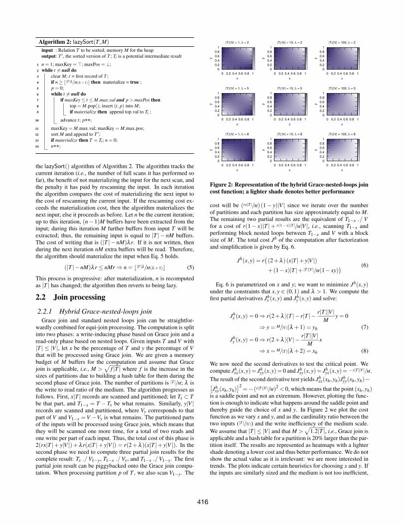
Figure 2: Representation of the hybrid Grace-nested-loops joincost function; a lighter shade denotes better performance

cost will be (rx|T |/M)(1− y)|V | since we iterate over the numberof partitions and each partition has size approximately equal to M.The remaining two partial results are the equivalent of T1−x ./ Vfor a cost of r(1− x)|T |+ r(1− x)|T |/M|V |, i.e., scanning T1−x andperforming block nested loops between T1−x and V with a blocksize of M. The total cost Jh of the computation after factorizationand simplification is given by Eq. 6.

Jh(x,y) = r((2+λ )(x|T |+ y|V |)+(1− x)|T |+ |T ||V |/M(1− xy)

) (6)

Eq. 6 is parametrized on x and y; we want to minimize Jh(x,y)under the constraints that x,y ∈ (0,1) and λ > 1. We compute thefirst partial derivatives Jh

x (x,y) and Jhy (x,y) and solve:

Jhx (x,y) = 0⇒ r(2+λ )|T |− r|T |− r|T ||V |

My = 0

⇒ y = M/|V |(λ +1) = yh (7)

Jhy (x,y) = 0⇒ r(2+λ )|V |− r|T ||V |

Mx

⇒ x = M/|T |(λ +2) = xh (8)

We now need the second derivatives to test the critical point. Wecompute Jh

xx(x,y)= Jhyy(x,y)= 0 and Jh

xy(x,y)= Jhyx(x,y)= − r|T ||V |/M.

The result of the second derivative test yields Jhxx(xh,yh)Jh

yy(xh,yh)−[Jh

xy(xh,yh)]2

=−(r|T ||V |/M)2 < 0, which means that the point (xh,yh)is a saddle point and not an extremum. However, plotting the func-tion is enough to indicate what happens around the saddle point andthereby guide the choice of x and y. In Figure 2 we plot the costfunction as we vary x and y, and as the cardinality ratio between thetwo inputs (|T |/|V |) and the write inefficiency of the medium scale.We assume that |T | ≤ |V | and that M >

√1.2|T |, i.e., Grace join is

applicable and a hash table for a partition is 20% larger than the par-tition itself. The results are represented as heatmaps with a lightershade denoting a lower cost and thus better performance. We do notshow the actual value as it is irrelevant: we are more interested intrends. The plots indicate certain heuristics for choosing x and y. Ifthe inputs are similarly sized and the medium is not too inefficient,

416

Standard hash join Lazy hash joiniteration reads writes reads writes savings penalty

1 m(M+MT ) (m−1)(M+MT ) m(M+MT ) 0 (m−1)(M+MT )λ r 02 (m−1)(M+MT ) (m−2)(M+MT ) m(M+MT ) 0 (m−2)(M+MT )λ r (M+MT )r3 (m−2)(M+MT ) (m−3)(M+MT ) m(M+MT ) 0 (m−3)(M+MT )λ r 2(M+MT )r

. . . . . . . . . . . . . . . . . . . . .i (m− i+1)(M+MT ) (m− i)(M+MT ) m(M+MT ) 0 (m− i)(M+MT )λ r (i−1)(M+MT )r

Table 1: The progress of standard hash join compared to lazy hash join

then we are better off using large values for x and y, i.e., employ-ing Grace join; this is intuitive as Grace join is more efficient thannested loops. If the inputs have similar sizes then the decisive factoris λ , the write to read ratio of the medium. As λ grows the advan-tage shifts to nested loops. On the other hand, as the ratio betweeninput sizes changes, we can start gradually employing nested loopsas the evaluation algorithm. This can be proportional, e.g., movingalong the diagonal of each individual plot, i.e., x ≈ y, as shown inthe middle row of plots of Figure 2; alternatively, choosing valuesin the bottom right triangular region of each plot, e.g., x+y = 1 andx≥ y is a good rule of thumb.

2.2.2 Segmented Grace joinLet us now assume that we do not account for each input inde-

pendently, but instead operate at a partition level. Given a numberof partitions k we choose to materialize only some number x ofthem and continuously iterate over the rest of the inputs to pro-cess the remaining k− x partitions. The algorithm first scans bothinputs and offloads k partitions. Assuming inputs T and V with|T | ≤ |V | and also assuming that our memory budget M is greaterthen

√f |T |, i.e., Grace join is applicable, then k = d|T |/Me. The

total cost Js of the algorithm is given by Eq. 9. The first two factorsaccount for Grace join. We scan the input to extract the x partitions;we offload these partitions; and then read them back to process theirpartial join. We therefore fully scan T and V and then write andread x(|T |+ |V |)/k buffers, where |T |/k (resp. |V |/k) is the size of eachpartition of T (resp. V ). The last factor is the cost of iterating overboth inputs k− x times to process the remaining partitions.

Js(x) = r(|T |+ |V |)+ rx(1+λ )

(|T |+ |V |

k

)+ r(k− x)(|T |+ |V |)

(9)

The cost is parametrized on x: the number of partitions that will bewritten. After factoring common terms, Eq. 9 can be rewritten as:

Js(x) = r(|T |+ |V |)(1+ (λ +1)x/k+ k(1− x))

The cost of Grace join is r(|T |+ |V |)(λ + 2); this algorithm per-forms better if 1+ (λ +1)x/k+ k(1− x)< λ +2 holds, or:

x <(λ +1− k)kλ +1− k2 (10)

Eq. 10 ensures that Segmented Grace join outperforms Grace join.Regardless of outperforming Grace join, the choice of x is a knobby which we alter the write intensity of the algorithm.

2.2.3 Lazy hash joinGiven M memory buffers and two inputs T and V with |T |< |V |,

standard hash join computes the join in k= d|T |/Me iterations by par-titioning the inputs in m partitions. During iteration i the algorithmscans T and hashes each t ∈ T to identify its partition. If t belongsto partition i, the algorithm puts it in an in-memory hash table. If tbelongs to any other partition it offloads it to the backing store. The

algorithm then scans V and hashes each v ∈ V to identify its par-tition. If v belongs to partition i it is used to probe the in-memoryhash table; any matches are propagated to the output. If t doesnot belong to partition i, it is offloaded to the backing store. Thealgorithm iterates as above until both inputs are exhausted. Thus,M buffers from T and MV = d|V |/ke buffers from V are eliminatedin each iteration. Assume now that the algorithm is lazy: whenit comes across a record that does not belong to the partition cur-rently being processed, it does not write it back. Instead, it pays thepenalty of rescanning the input during the next iteration.

In Table 1 we show the progression of the lazy algorithm com-pared to standard hash join. In each iteration the algorithm earnssavings; but doing so incurs a penalty during the next iteration. Thesavings in each iteration are equal to the portion of the input that isnot written (hence the multiplication with λ r). The penalty is equalto the portion of the input that would not have been read in com-parison to standard hash join. The algorithm is better off as long asthe savings surpass the penalty. When the savings are less than thepenalty plus the cost of materializing the part of the input that willbe processed in the remaining iterations, the algorithm should ma-terialize an intermediate input. Therefore, the iteration n at whichthe penalty surpasses the savings is computed through Eq. 11.

nr > (k−n)λ r⇒ n > k/(λ +1)⇒ n = bk/(λ +1)c (11)

The process is progressive. The algorithm periodically materializesintermediate inputs and then reverts to being lazy.

3. IMPLEMENTATIONOur implementation, shown in Figure 3, treats DRAM and per-

sistent memory as distinct levels of the memory hierarchy. Ouralgorithms operate at the DRAM level and offload data to persis-tent memory for later processing; thus, DRAM is the equivalent ofa bufferpool in a database system. Data is exchanged in cachelines(termed buffers in the algorithmic framework) between the two lev-els of memory. Our algorithms have a limited number of DRAMcachelines for their operation. A thin abstract persistence layersits between DRAM and persistent memory to implement persistentcollections: sources and/or intermediate results that the algorithmsoperate on. Persistent collections are organized in blocks that arelarger than cachelines to further amortize the persistent memory I/Ocost. However, the block size may well be equal to the cachelinesize if so desired. In what follows, we present the library supportneeded for implementing our algorithms. We then focus on thepersistence layer and give four methods to instantiate it.

3.1 Library supportAbstract API definition. The premise of write-limited algorithmsis that some intermediate results need not be materialized but canbe reconstructed from primary inputs. Therefore, we define an APIto expose such opportunities to the runtime. Our only assumptionis that every collection within a computation has a unique identi-fier. This can be enforced by the thin persistence layer of Figure 3.The materialization of any collection is by default deferrable unless

417

runtime algorithms

persistent collections

persistence layer

bufferpool

DRAM

persistent memory

cachelines

blocks

Figure 3: Implementation overview: a thin persistence layersits between a traditional two-level hierarchy. The runtime al-gorithms issue calls to the persistence layer, which in turn ap-plies them on collections hosted in persistent memory.

specified otherwise by the programmer. Collections that must bematerialized are tagged as such when they are declared. We have aspecial type of collection that is purely in-memory; such collectionsare also tagged as such at declaration time. Our API has the follow-ing calls: (a) split(T,n,Tl ,Th): split collection T at position ninto Tl and Th; (b) partition(T,h(),k,〈Ti〉,〈si〉= |T |/k): partitioncollection T into k partitions T1 to Tk using h() as the partitioningfunction; the size of each partition is expected to be s1 to sk respec-tively; the last argument is optional and if omitted each partition isexpected to be of size |T |/k; (c) filter(T, p(), f ,Tp): filter collec-tion T into Tp using predicate p() and expect the output to be of sizef |T | where f ∈ [0,1]; (d) merge(Tl ,Tr,m(),T ): merge collectionsTl and Tr into T using m() as the merging function. These primi-tives are enough to implement write-limited algorithms and enablethe runtime to perform the optimizations we have described. Thisis achieved by tracking collection sizes and read/write operations;and dependencies across primary and deferred collections.

T partitionhash(x) mod 3

T0

T1

T2

V partitionhash(x) mod 3

V0

V1

V2

mergeT0⋈V0

mergeT1⋈V1

mergeT2⋈V2

S

Figure 4: Example control flow graph

Runtime support. Totrack dependencies be-tween collections weemploy a control flowgraph. The nodes ofthe graph are eithercollections or one ofthe API calls. Edgesfrom collections to APIcall nodes mean thecollection is the call’sinput; outgoing edgesfrom API call nodes tocollections mean the collection is an output. Each API call nodeis annotated with call-specific parameters. When the collection isaccessed the runtime decides whether the collection should be ma-terialized or not. Simply declaring a collection and how it is con-structed does not materialize it; only access to a collection triggersits potential materialization. Upon access, the runtime estimates thenumber of reads and writes to construct the collection and decideswhether deferring materialization is cost-effective. To materializea collection we start from its oldest materialized ancestor and ap-ply all the computations that construct it. The runtime enforces theconstraint that no input is fully scanned twice to materialize its out-puts. For instance, consider a partition() operation where thematerialization of the first few output partitions is deferred. If uponaccess to a subsequent partition the runtime decides to materialize

it, then it must decide to materialize or defer all remaining parti-tions and materialize the selected ones while it scans the input.

An example control graph is shown in Figure 4. The graph cor-responds to the segmented Grace join algorithm of Section 2.2.1.Oval nodes are collections, while rectangular nodes are API calls.If a collection node’s oval is filled, then this collection is tagged asmaterialized. Empty collection nodes are deferred. In Figure 4 theinputs T and V are materialized, as is S, the final output of the com-putation. Inputs T and V pass through a partition() operation toproduce T0 − T2 and V0 −V2. Corresponding partitions are thenmerged through partial joins, with each partial result appended toS for the final output. Consider reconstructing V0: the runtime cando so by walking the graph. V0 depends on V so it can be recon-structed by partitioning V using function hash(x) mod 3, wherex ∈V . The estimated cost of the computation as it results from thegraph is r(|T |+ |V |)+ (w+ r)∑

2i=0 (|Ti|+ |Vi|)+ |S|w. Factoring

out the output materialization cost, and assuming a ratio λ = w/r,the decision of deferring materialization comes down to choosingthe number x of partitions to materialize. If we make the appropri-ate substitutions then the expression is rewritten as Eq. 9.Implementation and use of the API. The API calls and the con-trol flow graph act as a blueprint of an algorithm. Each algorithmmanifests as a physical operator and is assigned an operator con-text: an encapsulation of the information necessary to dynamicallyoptimize the operator. Collections accept an operator context as aconstruction parameter. The C++ fragment in Listing 1 showcasesthese properties. OpCtx is the operator context type. The API callsare members of the operator context, which has two more methods:assess() and produce(). Both methods accept as parameter theidentifier of a collection. The first method assesses the collection todecide whether it should be materialized; the second method pro-duces the collection. It does so by walking the control flow graph ofthe operator, as we will shortly see. Collections can be queried ontheir state (in-memory, materialized, or deferred). When a collec-tion is opened the operator context assesses if the collection shouldbe materialized. If so, the context produces the collection.

enum c s t a t u s t { MEMORY, MATERIALIZED , DEFERRED } ;c l a s s C o l l e c t i o n {p r i v a t e :

s t d : : s t r i n g m name ; / / c o l l e c t i o n nameOpCtx* m ctx ; / / o p e r a t o r c o n t e x tc s t a t u s t m s t a t u s ; / / c o l l e c t i o n s t a t u s

p u b l i c :C o l l e c t i o n ( c o n s t s t d : : s t r i n g& name , OpCtx* c t x = 0 ,

c s t a t u s t s = DEFERRED ) ;. . . } ;

void C o l l e c t i o n : : open ( ) {i f ( m s t a t u s == DEFERRED && m ctx ) { m ctx−>a s s e s s ( name ) ; }i f ( i s m a t e r i a l i z e d ( ) ) { m ctx−>produce ( name ) ; } }

Listing 1: Collection definition and access

Operators accept their context as a parameter when constructed.They provide a standard iterator interface, as well as an evaluate()method that records the control flow graph. This method is calledat construction time. The implementation of the method uses theAPI calls presented earlier, with the additional argument of the op-erator context. For example, the fragment of Listing 2 records thegraph of Figure 4. The SGJ class implements the algorithm as aphysical operator. Its evaluate() method sets up the workflow bydeclaring the appropriate collections for the partitions; the opera-tor’s context create name() method generates a unique identifier.After declaring collections, evaluate() makes an API call to thepartition() primitive passing the hashing function (a referenceto the hash of() functor) and the rest of the required parameters.Partitions are pairwise joined afterwards; this is done through an it-eration and successive merge() calls. One of the parameters to the

418

merge() call is the merging function. A functor implementing thisfunction is shown at the end of Listing 2. It overloads the C++ func-tion symbol and expects the two input and one output collections asparameters. The participating collections are opened so they can beassessed by the operator context and produced if necessary. Then,a hash table is built for the left collection and the right collection isused to probe the hash table for matches (omitted in the code).c l a s s O p e r a t o r {p r o t e c t e d :

OpCtx* m ctx ; . . .p u b l i c :

O p e r a t o r ( OpCtx* c tx , . . . ) : m ctx ( c t x ) , . . . {}v i r t u a l vo id e v a l u a t e ( ) = 0 ;

} ;c l a s s SGJ : p u b l i c O p e r a t o r { . . . } ;void SGJ : : e v a l u a t e ( ) {

/ / a s s u m p t i o n : m l e f t and m r i g h t are t h e two i n p u t s ;/ / m o u t p u t i s t h e o u t p u t c o l l e c t i o ns t d : : v e c t o r<C o l l e c t i o n*> l p ; s t d : : v e c t o r<C o l l e c t i o n*> rp ;f o r ( i n t i = 0 ; i < m p a r t i t i o n s ; i ++) {

l p . p u s h b a c k ( new C o l l e c t i o n ( m ctx−>c r e a t e n a m e ( ) ,m ctx , DEFERRED ) ) ;

rp . p u s h b a c k ( new C o l l e c t i o n ( m ctx−>c r e a t e n a m e ( ) ,m ctx , DEFERRED ) ) ; }

m ctx−>p a r t i t i o n ( m l e f t , h a s h o f ( m p a r t s ) , m pa r t s , l p ) ;m ctx−>p a r t i t i o n ( m r i g h t , h a s h o f ( m p a r t s ) , m pa r t s , rp ) ;f o r ( i n t i = 0 ; i < m p a r t i t i o n s ; i ++) {

m ctx−>merge (* l p [ i ] , * rp [ i ] , p a r t i t i o n j o i n ( ) , m ou tpu t ) ;} }

c l a s s p a r t i t i o n j o i n {void operator ( ) ( C o l l e c t i o n& l , C o l l e c t i o n& r , C o l l e c t i o n& s ) {

l . open ( ) ; r . open ( ) ; s . open ( ) ; / / a s s e s s and produce/ / b u i l d a hash t a b l e f o r lwhi le ( r . n e x t ( ) ) {

/ / probe f o r matches and o u t p u t i n t o s} } } ;

Listing 2: Example definition of an operator

Optimization. We track the accumulated numbers of reads andwrites per materialized collection during execution; and trigger ma-terialization by using rules. For each materialized collection, thesystem maintains a running sum of the number of read cachelinesfor that collection. The sum is used to decide if it is cheaper to keepa collection deferred and construct it on demand by (re)applyingoperations; or it is cheaper to materialize it. Rules rely on detectingpatterns stemming from the write optimizations of the algorithms.The rules are symbolically named and explained below:(a) multi-process: if a collection is processed multiple times then

it is materialized only if the number of times it is processedis greater than the write-to-read ratio; this rule applies to thesegmented and hybrid sort and join algorithms.

(b) eager-partition: if the system decides to materialize one of theoutputs of a partition() operation, then to amortize the writetime, all remaining results are materialized; this rule applies tothe segmented and hybrid join algorithms.

(c) process-to-append: intermediate results immediately appendedto another collection are always deferred.

(d) read-over-write: for a deferred collection, compare the cost,Cm, of materializing it to the so-far accumulated read cost, Cr,of its input, plus the read cost, Cc, for constructing it. If Cm ≤Cr +Cc then the collection is materialized and deferred in anyother case; this rule applies to the lazy sort and join algorithms.

Consider assessing T0 in Figure 4. Deferring it saves |T |/3 writes atthe cost of |T | reads; if |T |< λ |T |/3 where λ is the write/read ratio,T0 is deferred. When computing the partial join between T0 and V0the runtime knows, through the reference from a collection to itsoperator context, that T will be used to produce T0 by reapplyingthe partitioning function. Moving on to T1, the runtime compares2|T | to λ |T |/3 since we use the accumulated read cost for any mate-rialized source. If 2|T |> λ |T |/3, then T1 is materialized. If so, thenunder the eager-partition rule, the runtime materializes T2 as well.

Extensions. We presented the optimization of single operators.However, it is possible to generalize the method to entire evaluationplans, assuming that the operators are connected through interme-diate result collections. We have not tested this here as we focus onindividual algorithms rather than on entire queries. Incorporatingsuch functionality is straightforward but left for future work.

3.2 Incorporating persistent memoryA salient decision to make when incorporating persistent mem-

ory into the programming stack is whether to treat it as part of thefilesystem, or as part of the memory subsystem. The first optionfully addresses the persistence aspects, but implies the traditionalboundary between main memory and secondary storage. The sec-ond option makes persistent memory part of the memory hierarchytreated as volatile; thus the system itself must guarantee persis-tence. Our goal is not to answer the question of which option isbetter. Rather, it is to showcase the performance of our algorithmsunder each option. We tested our algorithms over four implemen-tation techniques, each driven by one of these options.RAM disk. The first approach is to employ a memory-mountedfilesystem. RAM disks are complete lightweight filesystems by-passing disk-related overheads. A RAM disk does not provide per-sistence between reboots, so it never incurs disk I/O; though it im-plements persistence semantics as long as the filesystem is mountedin main memory. A RAM disk bypasses the filesystem cache: writesand reads are synchronous to the portion of main memory allocatedto the RAM disk. Persistent collections in this case are standard filesand they are manipulated using filesystem calls. In typical filesys-tem fashion, files are organized in 512-byte records, which map tothe block abstraction of Figure 3. We can increase the block size inthe same way an operating system can increase the page size. Thisis a middle-of-the-road approach to bridging the mismatch betweentraditional block devices and byte-addressable persistent memory.The utility of this implementation is in identifying the pros andcons of using filesystem practices to access persistent memory.Byte-addressable filesystem. The second implementation wetested was a filesystem optimized for persistent memory. We usedIntel’s PMFS, the kernel-level filesystem extension available for theGNU Linux kernel version 3.9 onwards.1 Another option would bea filesystem like BPFS [5]. We decided to go for PMFS as it is akernel-level filesystem; BPFS is implemented in user space and thatcarries additional overhead. Kernel-level filesystems are tightly in-tegrated with the kernel and thus reduce the overhead of systemcalls, while, at the same time, allow the filesystem to access kernel-specific functionality. PMFS provides low-level fine-grained per-sistence primitives and implements file-level access through CPUload/store instructions, thereby minimizing overhead. Thus, PMFSpushes the file abstraction to its limits; doing away not only withoperating system caching, but also with the block-level interface.Dynamic arrays. The third option for a persistence layer is tosubstitute the runtime’s memory allocator (e.g., malloc()) withone that uses the non-volatile memory for allocations, as opposedto the system’s heap (see e.g., [4] for an approach). This affectsthe memory allocator, but not the way by which data structures al-locate memory. The typical data structure to represent an expand-able random-access collection of records is a dynamic array, or, inC++ terms, a vector. C++ vectors have an initial capacity; whenthat capacity is reached they allocate a memory chunk twice as bigas their current capacity; copy the elements over; and release thememory they had previously occupied. The doubling of allocatedmemory and, more importantly, the copying of elements over are

1Available at https://github.com/linux-pmfs.

419

characteristic valueprocessor Intel Xeon E5420 (four cores)

clock speed 2.5GHz per coreI1 cache 32kB per core

D1 cache 32kB per coreL2 cache 2×6MBmemory 12GB DDR2, fully buffered

Table 2: Hardware performance characteristics

far from ideal for persistent memory as they incur a large numberof writes. This is, however, how dynamic arrays work in most run-times (e.g., Java Vectors and ArrayLists operate similarly).Blocked memory. Finally, we implemented the persistence layeras a mix of the previous options. We kept the interface of a dynamicarray, but changed the memory profile of the array to a linked list ofmemory blocks. Accessor methods over the list of blocks providebyte addressability. Memory is allocated one block at a time withno copying upon expansion. This is effectively an in-memory filerepresentation without the overhead of persistence, whether that isprovided by the memory allocator or a filesystem substrate. Theonly overhead is reading from and writing to persistent memory.

4. EXPERIMENTAL STUDYImplementation and hardware. We developed our algorithmsin C++ and used the language’s template mechanisms to eliminateany artificial bloat associated with type genericity. This means thatfor any data field access we do not perform function calls to re-trieve values; we simply dereference a pointer, which aids the com-piler and the runtime to better optimize the code and its execu-tion. The code was compiled using g++ version 4.7.3 with the -O3optimization flag for maximum code efficiency. We used the 3.9GNU/Linux kernel, as the public version of PMFS is available forthat kernel source tree. Our hardware had the performance charac-teristics summarized in Table 2. Even though we used a quad-coreCPU our implementation was single-threaded and did not make anyuse of parallelism. Our tests did not perform any disk I/O apartfrom the necessary for loading the data before processing (whichwe have factored out in our reported timings). We tested block sizesranging from 512 bytes (the disk record size) to 8192 bytes. Wefound an improvement in response time of 10% on average whenmoving from 512 to 1024 bytes and insignificant improvements be-yond that. We therefore report measurements for 1024-byte blocks.Datasets and metrics. We developed a custom microbenchmarkof sort and join operations, as we wanted to test our techniques ina controlled environment and not in the context of a full databaseserver with the intricacies and complexity it introduces. We useda schema of ten eight-byte integer attributes for a total record sizeof 80 bytes. The key attribute followed the key value permutationof the Wisconsin benchmark [6]. The values of the remaining at-tributes were computed based on the key attribute through integerdivision and modulo computations. We instrumented the code toreport the response time, and the numbers of cacheline reads andwrites. For response time, we ran each operation ten times. Wereport the average; variance was less than 0.1%.Methodology. To simulate the read and write latencies of persis-tent memory we followed the lead of the hardware community [24]and injected artificial delays after read and write operations. Wedid so at a cacheline granularity. To enforce the delay we used thehardware counters to invoke an idle loop of as many clock ticks asnecessary for the desired latency. We used a 10ns read latency anda 150ns write latency [22, 24]; we further experiment with differentlatencies in the sensitivity analysis of Section 4.2.

5

6

7

8

9

10

11

10 20 30 40 50 60 70 80 90 100

response tim

e (

s)

memory size (MB)

5

10

15

20

25

30

35

40

45

response tim

e (

s)

ExMS

LaS

HybS, 20%

HybS, 80%

SegS, 20%

SegS, 80%

ExMS LaS HybS SegS

min writes (reads) 11.42 (11.42) 5.71 (34.47) 7.66 (16.00) 6.86 (12.38)max writes (reads) 11.43 (11.43) 5.90 (177.14) 9.82 (12.57) 7.92 (11.74)

Figure 5: Sorting performance for varying memory sizes;writes and reads in millions of cachelines

5

6

7

8

9

10

11

12

13

14

10 20 30 40 50 60 70 80 90 100

response tim

e (

s)

memory size (MB)

ExMS

dyn. array

RAM disk

PMFS

blocked memory

10

20

30

40

50

60

70

80

10 20 30 40 50 60 70 80 90 100

response tim

e (

s)

memory size (MB)

LaS

10 15 20 25 30 35 40 45 50 55 60

10 20 30 40 50 60 70 80 90 100

response tim

e (

s)

memory size (MB)

HybS, 20%

8

9

10

11

12

13

14

15

10 20 30 40 50 60 70 80 90 100

response tim

e (

s)

memory size (MB)

HybS, 80%

5 6 7 8 9

10 11 12 13 14 15

10 20 30 40 50 60 70 80 90 100

response tim

e (

s)

memory size (MB)

SegS, 20%

dyn. array

RAM disk

PMFS

blocked memory

4

6

8

10

12

14

16

10 20 30 40 50 60 70 80 90 100

response tim

e (

s)

memory size (MB)

SegS, 80%

Figure 6: Performance comparison of sorting algorithms underthe four different implementation alternatives

4.1 Performance analysisWe first compare the raw performance of the algorithms before

analyzing their sensitivity to parameter values. We will be doing sofor all four implementations and in a variety of settings.

4.1.1 SortingWe start with an analysis of our sorting algorithms over a ten-

million-record input. The algorithms are summarized as follows:(a) ExMS: standard external mergesort using replacement selec-tion; (b) SegS: segment sort (Section 2.1.1); (c) HybS: hybrid sort(Section 2.1.2); and (d) LaS: lazy sort (Section 2.1.3) We first testedthe impact of available main memory, as this affects the reductionin the number of writes. We varied the amount of available memoryfrom 1% to 15% of the total input size. SegS is parametrized onthe percentage of the input that will be sorted using external merge-sort; likewise, HybS is parametrized on the percentage of the mainmemory that is used as the selection region. We call these percent-ages the write intensity of each algorithm; the more write-intensivethe algorithm the better the performance, at the cost of extra writes.Performance comparison. In Figure 5 we report the response

420

time for each algorithm and in the bottom table we give the min-imum and maximum number of writes for each algorithm, alongwith the corresponding number of reads in parentheses. We fo-cus on the blocked memory implementation as it had the minimaloverhead (though we will return to this point shortly). We plot theresponse times of ExMS and LaS; and HybS and SegS for writeintensities of 20% and 80%; we will further analyze the impact ofwrite intensity in Section 4.2. We present the overall performanceof all algorithms and a zoomed in picture of the four best perform-ing algorithms as LaS and HybS for a 20% write intensity are dis-proportionately slow and make the performance differences of theremaining algorithms harder to see. Naturally, performance im-proves as more memory becomes available. Note that even thoughExMS is optimized for symmetric I/O, its write-limited competi-tion outperforms it from the beginning. For a small write intensityHybS and SegS incur about 35% fewer writes. As the write inten-sity grows the algorithms perform at most 15% fewer writes. HybShas comparable performance to ExMS; SegS outperforms HybSby about 30% on average. LaS has the worst response time. It has,however, the best write profile overall by performing about 50%fewer writes than ExMS and up to 30% fewer writes than the bestversion of SegS. Note also how the write-limited algorithms tradewrites for reads: as the number of writes decreases, the number ofreads increases. The exception is LaS which always performs ap-proximately the same (and minimal) number of writes; the reduc-tion in the number of reads is due to more memory being available(and hence longer sorted chunks being generated).Implementation comparison. In Figure 6 we show the overheadof each implementation; each layer in the stack graph representsadditional overhead. The blocked memory approach bears the min-imal overhead. Its only penalties are the write and read costs of per-sistent memory. The PMFS implementation approximates the mini-mal overhead. Exposing byte addressability to the filesystem seemslike a viable approach to introduce persistent memory functionalityin the processing stack. The next best performing implementationis the RAM disk one. Even though it bypasses the caching overheadof a filesystem, the remaining filesystem overheads and primarilyblock-level access, suggest that introducing byte addressability atthe filesystem level is crucial in order to use filesystem abstrac-tions for manipulating persistent collections. The worst-performingimplementation is the dynamic memory one. The reason is thewrite/read asymmetry of the medium is not exposed. Even thoughthis implementation is still a main-memory based one, i.e., it ex-hibits the same access overheads as blocked memory, its realloca-tion and data copying to improve memory access patterns result inexcessive writes; this in turn hurts performance. Even for a not aswrite-intensive an algorithm as SegS with a 20% write intensity,the overhead of the dynamic array implementation may be up to50% for low memory budgets; or go up to a factor of two for largermemory sizes. While the order of the implementations by perfor-mance merit is generally the same, there is one outlier: LaS. There,the memory-based approaches are better than the ones based on afilesystem. LaS bears the minimal number of writes. Thus, thenumber of expansion operations of the dynamic array is minimal,which in turn means that the write penalty is more-or-less amor-tized as it is not paid as frequently.

4.1.2 Join processingWe computed the join between a one-million-record (left) input

and a ten-million-record (right) one. Each left input record joinedwith ten right input records. The algorithms are abbreviated as:(a) GJ: standard Grace join; (b) HJ: simple hash join; (c) NLJ:nested loops join; (d) HybJ: hybrid Grace-nested-loops join (Sec-

tion 2.2.1); (e) SegJ: segmented Grace join (Section 2.2.2); and(f) LaJ: lazy join (Section 2.2.3). HybJ and SegJ are annotatedwith their write intensity. For HybJ this is the percentage of theleft and right inputs handled using Grace join; for SegJ this is thepercentage of the number of partitions materialized. For instance,HybJ, 50% - 80% means that 50% of the left input and 80% ofthe right input are handled using Grace join. The response time ison the y-axis and it is plotted against the available memory on thex-axis, which ranged from 1% to 15% of the left (smaller) input.Performance comparison. We first compare the performance ofthe two versions of HybJ and SegJ for a 50% write intensity acrossthe board; and the performance of LaJ; to NLJ, GJ and HJ in Fig-ure 7(a). The write-limited algorithms quickly catch-up to GJ, thebest performing I/O-optimized solution, and outperform it as avail-able memory grows. In Figure 7(b) we compare the performanceof HybJ to GJ. The performance of HybJ improves for differentcombinations of write intensity for its left and write inputs. Thewrite intensity over the right input dictates performance: the morewrite-intensive the processing of the right input, the quicker the al-gorithm catches up with GJ for a given amount of memory. At thesame time, one can have reasonable performance at a low write in-tensity over the right input. SegJ usually outperforms GJ and isonly suboptimal for a low write intensity or a low available mem-ory size, as shown in Figure 7(c). Note the tradeoff between writeintensity and memory: we can obtain good performance at a lowwrite intensity provided we are willing to use more memory. Fi-nally, we focus on LaJ, effectively a variant of HJ. As shown inFigure 7(d) LaJ always outperforms HJ by up to a factor of threefor small memory sizes. Also, it converges much sooner to theperformance of GJ and surpasses it as available memory grows.

In the bottom table of Figure 7 we show the minimum and maxi-mum cacheline writes of the algorithms, along with the correspond-ing number of reads in parentheses. It is evident that the write-limited algorithms perform fewer writes than the competition. Atthe same time, there is a tradeoff between writes and reads. Con-sider, for instance, an aggressive algorithm like SegJ at a low writeintensity like 20%: the number of reads for the maximum num-ber of writes is about one order of magnitude higher than the cor-responding figure for GJ. By reducing the number of writes by afactor of two, however, the algorithm exhibits better performanceoverall. This motif is evident for all write-limited algorithms: theyperform fewer writes than the competition, at times approximatingthe minimal number of writes that a read-intensive algorithm likeNLJ guarantees. At the same time, however, they exhibit an in-flated number of reads. But because of the write/read asymmetryof the medium this discrepancy does not compromise performance.Implementation comparison. The results for the algorithms ofFigure 7(a) and the four reference implementations are shown inFigure 8. The blocked memory implementation again has the small-est overhead, with the PMFS implementation closely following it.The dynamic memory implementation exhibits the highest over-head in the majority of cases, reaching up to a factor of two foran algorithm optimized for symmetric I/O like GJ. In general, theoverheads of the alternative implementations over the blocked mem-ory one are not always as high as was the case for sorting. For in-stance, the overhead is minimal for the SegJ algorithm with a 50%write intensity, or the LaJ algorithm as memory grows. This is nottrue for HybJ and a 50% write intensity over each input where theoverhead rises to 50% for the dynamic array implementation.

4.2 Sensitivity analysisWe now analyze the sensitivity of the algorithms to their parame-

ters. We begin with the write intensity, which is effectively a ‘knob’

421

0

10

20

30

40

50

60

70

80

90

1 2 3 4 5 6 7 8 9 10

resp

on

se

tim

e (

s)

memory size (MB)

(a) Overall

NLJ

HJ

GJ

LaJ

SegJ, 50%

HybJ, 50% - 50%

0

5

10

15

20

25

1 2 3 4 5 6 7 8 9 10

resp

on

se

tim

e (

s)

memory size (MB)

(b) HybJ compared to GJ

GJ

HybJ, 20% - 80%

HybJ, 50% - 50%

HybJ, 80% - 20%

0

5

10

15

20

25

1 2 3 4 5 6 7 8 9 10

resp

on

se

tim

e (

s)

memory size (MB)

(c) SegJ compared to GJ

GJ

SegJ, 20%

SegJ, 50%

SegJ, 80%

0

5

10

15

20

25

30

1 2 3 4 5 6 7 8 9 10

resp

on

se

tim

e (

s)

memory size (MB)

(d) LaJ compared to HJ, GJ

HJ

GJ

LaJ

GJ HJ NLJ HybJ, 20% - 80% HybJ, 50% - 50% HybJ, 80% - 20% SegJ, 20% SegJ, 50% SegJ, 80% LaJ

min writes (reads) 11.23 (11.31) 24.57 (25.14) 5.71 (97.71) 9.43 (39.54) 8.86 (21.78) 7.31 (68.46) 6.50 (44.90) 7.41 (34.86) 8.20 (29.03) 8.86 (42.14)max writes (reads) 14.00 (14.57) 173.43 (174.00) 5.71 (677.71) 10.40 (62.54) 9.66 (29.71) 8.46 (217.89) 7.88 (158.40) 8.10 (95.38) 9.21 (33.57) 12.48 (149.89)

Figure 7: Performance of the join algorithms; writes and reads in millions of cachelines

4

5

6

7

8

9

10

11

12

13

1 2 3 4 5 6 7 8 9 10

response tim

e (

s)

memory size (MB)

GJ

dyn. array

RAM disk

PMFS

blocked memory

0

20

40

60

80

100

120

140

160

1 2 3 4 5 6 7 8 9 10

response tim

e (

s)

memory size (MB)

HJ

20

40

60

80

100

120

140

1 2 3 4 5 6 7 8 9 10

response tim

e (

s)

memory size (MB)

NLJ

2

4

6

8

10

12

14

16

18

20

1 2 3 4 5 6 7 8 9 10

response tim

e (

s)

memory size (MB)

HybJ, 50% - 50%

0

5

10

15

20

25

30

35

40

45

1 2 3 4 5 6 7 8 9 10

response tim

e (

s)

memory size (MB)

SegJ, 50%

0 5

10 15 20 25 30 35 40 45 50

1 2 3 4 5 6 7 8 9 10

response tim

e (

s)

memory size (MB)

LaJ

dyn. array

RAM disk

PMFS

blocked memory

Figure 8: Performance comparison of join algorithms underthe four different implementation alternatives

8

10

12

14

16

18

20

22

10 20 30 40 50 60 70 80 90

response tim

e (

s)

percentage of write intensity

HybS, blocked memory

HybS, PMFS

HybS, RAM disk

HybS, dyn. array

SegS, blocked memory

SegS, PMFS

SegS, RAM disk

SegS, dyn. array

Figure 9: Impact of write-intensity on sorting algorithms

for specific algorithms. We then present the impact of the system-wide write/read asymmetry and the effectiveness of our cost model.

4.2.1 Impact of write intensityFor some algorithms, write intensity is tunable: it can either be

chosen so that the algorithm is cost-optimal; or to bound the num-ber of writes each algorithm performs with respect to its symmetric-I/O counterpart. In Figure 9 we report the impact of write intensityon the two sorting algorithms affected by this choice, i.e., SegS andHybS. We report this impact on the four persistent memory imple-mentations. The first conclusion is that the impact of write intensityis not as high on SegS as it is on HybS. The write intensity of SegSaffects only the percentage of the input sorted using external merge-

4

6

8

10

12

14

16

18

10 20 30 40 50 60 70 80 90

response tim

e (

s)

percentage of write intensity

SegJ

HybJ, x - 20%

HybJ, x - 50%

HybJ, x - 80%

HybJ, 20% - x

HybJ, 50% - x

HybJ, 80% - x

Figure 10: Impact of write-intensity on join algorithms

sort, with selection sort used for the rest of the input. This reducesthe number of writes overall, but does not result in larger gains asintensity increases; SegS quickly reaches good performance at alower intensity. Write intensity has a more pronounced effect onHybS. As write intensity grows, the performance of the algorithmimproves substantially by up to 45%; SegS is only improved by upto 18%. Note the substantial overlap between the different algo-rithms, their write intensity, and the choice of implementation. Forinstance, for a low write intensity, even the worst implementationof SegS beats HybS on performance.

Switching to join evaluation, in Figure 10 we show the impactof write intensity on SegJ and HybJ, which are affected by thischoice. HybJ is parameterized on the write intensity over each in-put individually. To aid presentation we keep the write intensityover one input constant and scale write intensity over the other;e.g., HybJ, 50% - x denotes a 50% write intensity over the leftinput as we scale the write intensity over the right input. We reportonly for the blocked memory implementation as it carries the low-est overhead and to avoid cluttering the plots. The impact of writeintensity on SegJ is gradual, with each increment improving per-formance up to about 20% in the end. For HybJ the determiningfactor is the write intensity over the left input. The performancefor a fixed write intensity over the left input as write intensity overthe right input varies is relatively stable. But as the write inten-sity of the left input grows, performance improves substantially toa maximum gain of up to 50%. This is due to the write intensity ofthe left input dictating the portion of the computation that will beperformed with nested loops, or, more specifically, the number offull passes over the larger right input. The higher the intensity, thesmaller the number of passes; and the better the performance. Notethat a large write intensity is not necessary: a 50% write intensityover the left input is enough to give good performance. As the leftinput is the smaller one, this results in substantial write savings.

4.2.2 Impact of write/read ratioWrite-limited algorithms are designed for asymmetric write/read

costs. We measured the performance of the algorithms by varyingthe write latency from 50ns to 200ns. We chose not to test different

422

7

8

9

10

11

12

13

14

15

16

17

40 60 80 100 120 140 160 180 200

response tim

e (

s)

write latency (ns)

LaS

HybS, 20%

HybS, 50%

SegS, 20%

SegS, 50%

9

10

11

12

13

14

40 60 80 100 120 140 160 180 200

response tim

e (

s)

write latency (ns)

HybJ, 50% - 20%

HybJ, 50% - 50%

SegS, 20%

SegS, 50%

LaJ

Figure 11: Impact of write latency on selected sorting (left) andjoin (right) algorithms

read latencies as read performance of persistent memory is gener-ally good and does not vary as widely—nor is it the major point weaddress in this work. The performance of selected runs are shownin Figure 11 for sorting and join algorithms (left and right plotsrespectively). We report only for the blocked memory implementa-tion as it carries the minimal overhead. We focus on no more thana 50% write intensity to avoid further penalizing the write profileof the algorithms. The write-limited algorithms are not adverselyaffected by higher write latencies. Even though write latency in-creases by up to 100% between successive points, the hit on per-formance is no more than 5%. The results confirm the resilience ofour algorithms to write/read asymmetry.

4.2.3 Cost model validation

0.94

0.95

0.96

0.97

0.98

0.99

1

2 4 6 8 10 12 14

concord

ance (

Kendall’

s τ

)

available memory (percentage of the (left) input size)

sorting - all

join processing - all

sorting - write-limited

join processing - write-limited

Figure 12: Concordance betweenestimated and true performance

We have so far focusedon the performance of write-limited algorithms. For thesealgorithms to be useful, how-ever, they must be accompa-nied by a cost model captur-ing their performance. Wewill now validate in a lim-ited setting the cost expres-sions of the write-limited al-gorithms. We used the ten-million-record sorting input and the one-million by ten-million-record join computation as we varied memory for a fixed 150nswrite latency. We excluded the lazy algorithms, LaS and LaJ, fromthis study as their decisions are dynamic rather than static. That is,they monitor writes and reads and decide to materialize temporaryresults during run-time; in contrast to an optimizer deciding the bestchoice of algorithm at query compilation time. For each remainingalgorithm, for each sort and join benchmark, and for each mem-ory increment we estimated the cost of the algorithm using the costexpressions of Section 2, and ranked the algorithms according totheir estimated performance. We then executed the algorithms andranked them according to their true performance. We compared thetwo rank orders using Kendall’s τ correlation coefficient [12]. Thelatter captures the agreement between two different orderings of alist of elements by looking at the concordant and discordant pairsof ranks for the same element. The correlation coefficient is a num-ber in [−1,1] with 1 denoting complete agreement; −1 denotingcomplete disagreement; and 0 implying independence.

We report the correlation coefficient in Figure 12 as we scale theamount of available memory as a percentage of the total input size(for sorting) or the left input size (for join processing). We showconcordance for two cases per class of algorithm: if all algorithmsare included (i.e., algorithms optimized for symmetric I/O are usedtoo) or if we focus only on write-limited algorithms. There is al-ways high concordance between the estimated rank and the truerank. Concordance diverges as available memory grows since mostalgorithms then have comparable performance, thereby increasing

the likelihood of a mistake. Concordance is higher for join pro-cessing than sorting as there is greater variation in performanceand the cost expressions manage to differentiate between choicesmore effectively. Focusing only on the write-limited algorithmsimproves concordance for both sorting and join processing algo-rithms. This is due to: (a) fewer rank combinations being possible,and (b) the excluded algorithms always participating in groups ofsimilarly performing algorithms; both factors result in higher con-cordance. Concordance is always above the 0.94 mark indicatingthat the cost estimates truly capture the relative performance of thealgorithms and can be used as a solid basis for decision making.

4.3 DiscussionThe results affirm that choosing algorithms or implementations

when incorporating persistent memory into the I/O stack is notstraightforward. It is a combination of various parameters and itcomes down to what we want to optimize for. The algorithmsdo well in introducing write intensity and giving the developer, orthe runtime, a knob by which they can select whether to minimizewrites; or minimize response time; or both. It is also important thatthe majority of algorithms converges to I/O-minimal behavior at alow write intensity; e.g., SegS and SegJ approximate or outperformtheir counterparts optimized for symmetric I/O from a 20% writeintensity onwards. This confirms that one can have write-limitedalgorithms without compromising performance.

The cost models of the algorithms are necessary to choose analgorithm in an informed way. But it is not only the cost modelsthat are important. The API of Section 3.1 is also conducive, asit allows the developer to defer decision making at compile-time;rather, decisions can be made at run-time. Perhaps even by opti-mizing for different objectives at different times, making it possibleto autotune performance according to system-wide and potentiallyevolving policies; in addition to boosting performance during de-velopment if objectives are known a priori.

The results also suggest that one is better off using a memoryrepresentation for collections that borrows aspects of blocked stor-age and is not only optimized for main memory use. Considerthe dynamic array representation of collections, which is optimizedfor main memory use by increasing spatial locality; and leveragingtemporal locality to maximize performance. While array expansionin a main memory setting bears a one-off cost that is dwarfed by thebenefits of improved locality, this is no longer the case for persistentmemory and its asymmetric write/read costs. Thus, an implemen-tation optimized for main memory is not the best choice for per-sistent memory. Treating persistent memory as block-addressablestorage albeit mounted in main memory is not the best option ei-ther as it introduces significant overhead. A persistent collectionimplementation based on blocked memory shows the true potentialof the hardware and the algorithms as it effectively bears zero over-head apart from the unavoidable penalties due to the write/read costasymmetry. Whereas an implementation over a byte-addressablefilesystem like PMFS gives the best of both worlds: true file-likepersistence over a byte-addressable substrate at a low overhead inthe majority of cases. It therefore makes sense to strive to optimizesuch implementations and further reduce their overheads. This canbe achieved perhaps by additional hardware support, or better im-plementations of primitives. The goal should be to reach the idealperformance of blocked memory.

Finally, note that we studied asymmetry in terms of I/O responsetime. Asymmetry, however, also manifests in terms of power con-sumption [2]; or device degradation. Our algorithms are applicablethen as well and the relative gains may be higher as the asymmetryis more pronounced under such metrics.

423

5. RELATED WORKWith persistent memory only now starting to emerge as a stor-

age medium, related work in the area is rather limited. The clos-est area of research is flash memory, which has received consider-able attention. There has been a host of techniques on improvingthe performance of the flash translation layer (FTL), which is thepart of the flash controller that provides logical-to-physical addressmapping, power-off recovery, and wear-leveling. Researchers havestudied the FTL algorithms [3] and proposed various improvementson their performance based on block-level associativity [15], on-chip caching [1], page-level lazy updates [18], or wear-leveling [11].On the software side, research has focused on flash-specific buffer-pool management schemes [14, 16, 20, 21], query evaluation tech-niques [7, 19, 23], and logging [8]. This work, while relevant, doesnot cater for byte addressability. The differences in block- vs. byte-level access suggest that considerable effort will be necessary toport these approaches to persistent memory.

In a database context, Chen et al. [2] explored how database al-gorithms need to be changed in the presence of persistent memory.They argued for a radical reimplementation of algorithms by elim-inating data copying and using pointers to data in order to reducememory stores. Our stance is different: we argue that we are bet-ter off limiting writes at a higher level. To that end we give waysto limit writes at the system and developer levels by exposing theworkings of the algorithm through our API. The techniques of [2]then become orthogonal and may further improve performance.

The systems community has also addressed the persistence as-pects of persistent memory. Coburn et al. [4] look to support heap-based allocation operations on non-volatile media; our abstractionof persistent collections may certainly benefit from such allocationprimitives. Volos et al. [24] deal with the efficiency issues of sup-porting persistence and argue for a lightweight approach; this is acomplementary issue to what we address here as it targets the per-sistent memory controller rather than the software side of the sys-tem. Finally, Condit et al. [5] discuss the intricacies of designinga persistent byte-addressable filesystem; we have used similar con-cepts in our implementation of persistent collections over PMFS.

6. CONCLUSIONS AND OUTLOOKPersistent memory has the potential to become a universal stor-

age device. We addressed some of the issues involved in incorpo-rating persistent memory into database query engine design. Wefocused on two fundamental query evaluation operations, namelysorting and join processing. We adapted these operations for per-sistent memory and presented a family of write-limited algorithmsthat either minimize I/O; or are tunable by the developer and/orthe system during run-time. We presented API and implementationprimitives that enable the seamless integration of persistent mem-ory into the processing stack of database systems. We extensivelystudied the performance of our proposals. Our results showed thatwrite-limited algorithms deliver on their promise and outperformor, at worst, match the performance of traditional solutions.

One might extend this work to generalized algorithms (e.g., [9]);or data structures (e.g., indexes); or operations (e.g., aggregation).Alternatively, one might focus on persistent-memory-specific solu-tions to support other aspects of database systems like transactionprocessing and recovery. In this work, we have studied an inclusivememory hierarchy where data is moved from persistent memory toDRAM to be processed. It would be interesting to see the trade-offs involved in using only persistent memory and doing away withDRAM altogether. This becomes especially important if the latencyof persistent memory matches that of DRAM.

AcknowledgmentsThe author would like to thank the anonymous reviewers for theircomments. This work was supported by the Intel University Re-search Office and the Software for Persistent Memories program.

7. REFERENCES[1] A. Birrell et al. A design for high-performance flash disks.

SIGOPS Oper. Syst. Rev., 41(2), 2007.[2] S. Chen et al. Rethinking database algorithms for phase

change memory. In CIDR, 2011.[3] T.-S. Chung et al. System software for flash memory: A

survey. In EUC, 2006.[4] J. Coburn et al. NV-heaps: making persistent objects fast and

safe with next-generation, non-volatile memories. InASPLOS XVI, 2011.

[5] J. Condit et al. Better I/O through byte-addressable,persistent memory. In SOSP, 2009.

[6] D. J. DeWitt. The Wisconsin Benchmark: Past, Present, andFuture, 1993.

[7] J. Do and J. M. Patel. Join processing for flash SSDs:remembering past lessons. In DAMON, 2009.

[8] R. Fang et al. High performance database logging usingstorage class memory. In ICDE, 2011.

[9] G. Graefe. New algorithms for join and grouping operations.Computer Science - R&D, 27(1):3–27, 2012.

[10] B. K. Haddon. Cycle-sort: A linear sorting method. TheComputer Journal, 33(4):365–367, 1990.

[11] X.-Y. Hu et al. Write amplification analysis in flash-basedsolid state drives. In SYSTOR, 2009.

[12] M. Kendall. A New Measure of Rank Correlation.Biometrica, 30:81–89, 1938.

[13] L. Kevin et al. Disaggregated memory for expansion andsharing in blade servers. In ISCA, 2009.

[14] H. Kim and S. Ahn. BPLRU: a buffer management schemefor improving random writes in flash storage. In FAST, 2008.

[15] J. Kim et al. A space-efficient flash translation layer forCompactFlash systems. Trans. on Consumer Electronics.,2002.

[16] I. Koltsidas and S. D. Viglas. Flashing up the storage layer.PVLDB, 1(1), 2008.

[17] I. Koltsidas and S. D. Viglas. Data management over flashmemory. In SIGMOD, 2011.

[18] D. Ma et al. LazyFTL: A page-level flash translation layeroptimized for nand flash memory. In SIGMOD, 2011.

[19] D. Myers. On the use of NAND flash memory inhigh-performance relational databases. Master Thesis, MIT,2007.

[20] Y. Ou et al. CFDC: a flash-aware replacement policy fordatabase buffer management. In DAMON, 2009.

[21] S. Park et al. CFLRU: a replacement algorithm for flashmemory. In CASES, 2006.

[22] M. K. Qureshi et al. Phase Change Memory: from devices tosystems. Morgan & Claypool Publiishers, 2012.

[23] D. Tsirogiannis et al. Query processing techniques for solidstate drives. In SIGMOD, 2009.

[24] H. Volos et al. Mnemosyne: lightweight persistent memory.In ASPLOS, 2011.

424