WTP for Water Quality Improvements - UCL - London's … · The field work underlying this paper was...

WILLINGNESS TO PAY FOR WATER QUALITY MAINTENANCE

IN CHINESE RIVERS

by

Brett Day and

Susana Mourato

CSERGE Working Paper GEC 98-

WILLINGNESS TO PAY FOR WATER QUALITY MAINTENANCE

IN CHINESE RIVERS

by

Brett Day and

Susana Mourato

Centre for Social and Economic Research on the Global Environment University College London

and University of East Anglia

Acknowledgements The Centre for Social and Economic Research on the Global Environment (CSERGE) is a dedicated research centre of the Economic and Research Council (ESRC).

The field work underlying this paper was funded by WS Atkins International Limited, under the China Rural Project (RUWEP) of the UK Department for International Development (DfID). Susana Mourato gratefully acknowledges a grant provided by the Portuguese Junta Nacional de Investigação Científica e Tecnológica (JNICT) through the PRAXXIS XXI Programme. The authors are indebted to Nick Oxley for valuable comments and insights. Valuable contributions to the field work were also made by the staff from the Beijing Normal University and from the National Environmental Protection Agency (NEPA) of China. ISSN 0967-8875

Abstract Industrial expansion around Beijing in China has resulted in the increasing pollution of surface waters. This paper reports on the application of a contingent valuation survey to determine the value to the Beijing population of maintaining river water quality in one or all the rivers in the region. The survey revealed that the values that the population have for clean river water include a considerable non-use element. The valuation question included a referendum question to determine whether respondents were willing to pay anything to maintain river water quality. Those expressing a positive willingness to pay (WTP), faced a double-bounded dichotomous choice valuation question. The data are analysed using a combined spike model and willingness to pay model, in which the most appropriate form for the underlying WTP distribution is determined using the Box-Cox transformation. The average annual household WTP to maintain water quality in all the rivers around Beijing is found to be significantly higher than for any individual river, showing that respondents are sensitive to the scale of the proposed water quality improvements.

1

1. Introduction This paper reports on the results of a contingent valuation survey on valuing water quality improvements in the Beijing Metropolitan Region carried out as part of the China Rural Water Project. In this context, the purpose of the study was threefold:

• to estimate the willingness to pay of residents of the Beijing Metropolitan Region for water quality improvements in local rivers. Willingness to pay is a monetary measure of the benefits that residents in the target area derive from river water quality improvements. In particular, the study aims to assess (i) whether the value of water quality changes in a group of rivers is significantly different (higher) from the value of changes in a subset of those rivers (scale test); and (ii) whether the value of water quality changes significantly varies across rivers.

• to investigate the perceptions and attitudes of Beijing residents towards the preservation of rivers. This information helps identifying the motivations behind individual valuations and explaining differences in values across individuals.

• to investigate the feasibility of applying non-market valuation techniques to estimate the value of surface water quality changes in China and to explore the best way of structuring and conducting such studies.

The remainder of the paper is organised as follows:

• Section 2 explains the conceptual framework for the valuation exercise;

• Section 3 describes the questionnaire that was used to collect information;

• Section 4 discusses the fieldwork;

• Section 5 presents the results relating to socio-economic characteristics, attitudes and behaviour;

• Section 6 presents the willingness to pay results;

• Section 7 draws out the conclusions and explores their implications.

2

2. Conceptual Overview

2.1. Methodology Water quality improvements in surface waters generates a wide variety of market and non-market benefits. For the particular case of rivers in the Beijing Region, benefits include direct on-site uses, comprising mainly in-stream and off-stream recreation (swimming, boating, beach sports, sun-bathing, sightseeing, hiking/walking, angling, amenity values from the surrounding environment) and indirect use values, such as increased employment because of tourism or pleasure from reading or seeing pictures of the rivers. Water quality improvements may also produce a different type of benefits known as ‘non-use values’ that correspond to a wide range of motivations for which individuals might value environmental improvements in rivers irrespective of their use of it: benefits from protecting river quality for future generations (bequest values), from knowing that other people may enjoy cleaner river (altruistic values) or simply from the knowledge that rivers are being preserved for their own sake, providing a natural habitat for fish, plants and wildlife (existence values). In addition, between use and non-use values are the so called ‘option values’ that refer to benefits arising from guaranteeing the opportunity to use the rivers at a future date. The economic evaluation of rivers and lakes has traditionally focused on the demand for on-site recreation use. However, non-use values may play as important a role in justifying expenditures in water protection as the more conventional use benefits. This study estimates the total benefits for local residents of improving water quality levels in Beijing rivers. The question is how to estimate this total value. Many of the benefits described above are not traded in the market and hence cannot be valued by looking at market prices. To resolve this problem, economists have developed special techniques for placing monetary values on ‘non-market’ goods and services. In recent years, one such technique, the contingent valuation method (CVM), has gained widespread acceptance among both academics and policy makers as a versatile and complete methodology for benefit estimation (Mitchell and Carson, 1989). This study uses the contingent valuation method to estimate the value of changes in river water quality in the Beijing Region. CVM is a survey-based methodology. The basic underlying idea is that, by means of an appropriately designed questionnaire, a hypothetical market is described where the good in question can be traded. People are then directly asked to express their

3

maximum willingness to pay (WTP) for a hypothetical change in the level of provision of the good. In line with standard economic analysis, willingness to pay is considered to be the appropriate measure of the value which a person derives from a particular good, corresponding to the correct monetary welfare measures, namely Hicksian compensating and equivalent variations. This is because it forces people to take into account the fact that they are being asked to sacrifice some of their limited income to secure the good, and must thus weigh-up the value of what is being offered to them against alternative uses of that income. In this sense, willingness to pay is a much more powerful measure of value than a more general attitudinal question. While people may say, in response to an attitudinal question, that they ‘care about’ many things, in practice they will only be able to pay for a much smaller subset of these things. Furthermore, given that the focus of this study is the estimation of total benefits from river protection in Beijing, the adoption of the contingent valuation method is warranted by the fact that it is the only technique theoretically capable of estimating all the range of benefits produced by water quality improvements, including non-use values.

2.2. Overview of related studies

In recent years, CVM has been extensively applied in both developed and developing countries to the valuation of a wide range of environmental goods and services. Much of the impetus to this acceptance were the conclusions of the special panel appointed by the US National Oceanic and Atmospheric Administration. The panel concluded that CVM studies could produce estimates reliable enough to be used in a judicial process of natural resource damage assessment. In particular, CVM has been successfully applied to a variety of water related issues including sanitation, water supply, in-stream and off-stream recreation, flow enhancement and health risks. It has also been used in very different contextual frameworks: lakes and rivers, groundwater, bathing water (both salt and freshwater), fishing sites, urban water parks, wetlands and marine and coastal areas. However, existing water related valuation exercises in developing countries have concentrated primarily in two areas: water supply and sanitation. Studies of surface water quality such as the present study are scarce. In fact, it may not be obvious at first why resources should be spent in estimating the monetary value of surface water quality improvements in developing countries where households may not have access to more fundamental services like basic sanitation or water supply. The answer may lie precisely in the need to correctly

4

estimate demand for services like sanitation, as an inefficient or non-existent sanitation system invariable leads to increased surface water pollution. Moreover, in many cases, WTP studies of sanitation demand in developing countries estimate values that are so low that cost recovery is not feasible. The reason for this low demand lies, not only on a low ability to pay, but also on an incomplete perception of the benefits arising from installation of improved sanitation systems. One such benefit is improving surface water quality. In many cases, citizens of developing countries are concerned with pollution levels of rivers and lakes; had they been aware of the link between lack of domestic wastewater treatment and increased river pollution, their WTP for sanitation might have been different (higher). But uncovering the true value of wastewater treatment is not the only or even the more important reason why it is important to estimate the value of surface water quality improvements in developing countries. In many cases, surface waters are very polluted, directly affecting all those who use it for recreation or subsistence. The potential for tourism is undermined and all the range of indirect, option and non-use values described above are negatively affected. Table 1 provides an overview of selected contingent valuation studies estimating benefits from water quality improvements in surface waters in both developing countries and transitional economies. In both cases, given the distinguishing features of these economies, the success of CVM techniques depends crucially on careful design and implementation. The results from the current study do not have to be similar to those reported in Table 1; not only the local situations are completely distinct but also the survey instruments are different. Nevertheless, it is interesting to note that, in at least four of the above studies, WTP for water quality improvements amounts to less than 1% of household income. Of particular interest is the Chinese case-study reported in Table 1, a very basic willingness and ability to pay survey of water supply and sanitation in Kunming City, province of Yunnan. In fact, this is not really a contingent valuation study but a series of WTP questions. As a secondary output, the survey also included a question about WTP to help cleaning up Lake Dianchi (neither the payment vehicle nor the mechanism through which the clean-up would be achieved were specified). Some additional results are reported below as they may allow an interesting comparison with the estimates from the present study.

• 87% of respondents were concerned with the condition of Lake Dianchi and 75% would be prepared to pay 8.5 Yuan per month (102 Yuan per year) to clean it. Overall, this corresponds to a WTP of 6.4 Yuan per month or 77 Yuan per year. Estimated mean gross household income is 15,516 Yuan per year. Hence the WTP is about 0.5% of household income.

5

• 72% of respondents with piped water (84% of the total) were willing to pay an additional 11.9 Yuan per month for better water quality. Only 10% of those not connected were willing to pay 5.2 Yuan. Overall, the average WTP is 7.3 Yuan per month or 87.6 Yuan per year (0.6% of household income).

• 57.3% of respondents with indoor WC’s (43% of the sample) were prepared to pay 6.8 Yuan per month for an improved sewerage system. Only 9% of those without indoor WCs wanted to connect at a mean monthly charge of 9.1 Yuan. Overall, the average WTP is 2.1 Yuan per month or 26 Yuan per year (0.17% of household income).

Overall, these studies suggest that WTP for water quality improvements in developing countries is positive, although typically amounting to less than 1% of household income. Table 1: Selected contingent valuation studies of surface water quality in

developing countries and transitional economies

Case-study Characteristics Comments Authors

WTP to reduce coastal water pollution,

Barbados

1988/PI/ 709/ WTP/ DC / water bill/ / On

and off-site/ Tests

Mean annual WTP of US$11 (off-site) and

US$178 (on-site)

McConnell and Ducci (1989)

WTP to reduce coastal water pollution in

Montevideo, Uruguay

1989/PI/ 1500/ WTP/ DC / tax/ Off-

site/ Tests

Mean annual WTP of US$14 (<1% of median

household income)

McConnell and Ducci (1989)

WQ improvements in rivers and sea near

Davao City, Philippines

1992/ PI/ 777/ WTP/ OE and DC / tax/

Off-site/ Tests

Mean annual WTP of US$12-21 (0.5-1% of

household income)

Choe et al. (1994)

WQ improvements at Lake Dianchi, China

1995/PI/ 470/ WTP/ OE / tax/ Off-site/

No Tests

Mean annual WTP of 77 Yuan (0.5% of gross

household income)

Institute of Rural

Economy (1995)

Benefits of reducing eutrophication in the Baltic Sea and Coast,

Poland

1994/ PI/ 441/ WTP/ OE and DC/ tax/ On

site/ No tests

Substantial annual WTP larger than an average

monthly income!

Zylicz et al. (1995)

WQ improvements in Lake Balaton, Hungary

1995/ PI/ 1831/ WTP/ OE and DC/ tax/ On and off site/

Tests

Annual WTP of US$ 27 (1% of net annual

income)

Mourato (1998)

Notes: (i) WQ = water quality (ii) Characteristics: survey year/ personal interview (PI)/ sample size/WTP format/elicitation format: open-ended (OE), dichotomous choice (DC)/ payment vehicle: tax or water bill/ sample type: on or off-site/ Tests for bias

6

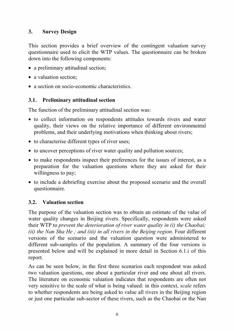
3. Survey Design This section provides a brief overview of the contingent valuation survey questionnaire used to elicit the WTP values. The questionnaire can be broken down into the following components:

• a preliminary attitudinal section;

• a valuation section;

• a section on socio-economic characteristics.

3.1. Preliminary attitudinal section

The function of the preliminary attitudinal section was:

• to collect information on respondents attitudes towards rivers and water quality, their views on the relative importance of different environmental problems, and their underlying motivations when thinking about rivers;

• to characterise different types of river uses;

• to uncover perceptions of river water quality and pollution sources;

• to make respondents inspect their preferences for the issues of interest, as a preparation for the valuation questions where they are asked for their willingness to pay;

• to include a debriefing exercise about the proposed scenario and the overall questionnaire.

3.2. Valuation section

The purpose of the valuation section was to obtain an estimate of the value of water quality changes in Beijing rivers. Specifically, respondents were asked their WTP to prevent the deterioration of river water quality in (i) the Chaobai; (ii) the Nan Sha He ; and (iii) in all rivers in the Beijing region. Four different versions of the scenario and the valuation question were administered to different sub-samples of the population. A summary of the four versions is presented below and will be explained in more detail in Section 6.1.i of this report. As can be seen below, in the first three scenarios each respondent was asked two valuation questions, one about a particular river and one about all rivers. The literature on economic valuation indicates that respondents are often not very sensitive to the scale of what is being valued: in this context, scale refers to whether respondents are being asked to value all rivers in the Beijing region or just one particular sub-sector of these rivers, such as the Chaobai or the Nan

7

Sha He. The chosen question design permits an investigation of sensitiveness to scale in the case of Chinese rivers, i.e. whether the value of one river is significantly different from the value of all rivers. It also allows an assessment of differences in values across individual rivers. VERSION 1: Scenario: ALL rivers in the Beijing Region deteriorate. First Valuation Question: WTP to maintain the quality of water ONLY in Chaobai. Second Valuation Question: WTP to maintain the quality of water in ALL rivers.

VERSION 2: Scenario: ALL rivers in the Beijing Region deteriorate. First Valuation Question: WTP to maintain the quality of water ONLY in Nan Sha He. Second Valuation Question: WTP to maintain the quality of water in ALL rivers.

VERSION 3: (reverse of Version 2) Scenario: ALL rivers in the Beijing Region deteriorate. First Valuation Question: WTP to maintain the quality of water in ALL rivers. Second Valuation Question: WTP to maintain water quality ONLY in Nan Sha He

VERSION 4: Scenario: ONLY the Nan Sha He deteriorates. First Valuation Question: WTP to maintain water quality ONLY in the Nan Sha He.

After having described a scenario and a hypothetical market, there are basically two ways of eliciting the willingness to pay for the specified change:

• respondents can be simply asked directly how much they would be willing to pay—this is known as open-ended elicitation. Sometimes, to aid the process of valuation, respondents are shown a range of amounts and asked to pick the one that best corresponds to their maximum WTP (‘payment card’ approach).

8

• respondents can be asked whether or not they would be willing to pay a specific amount £X, to which they might answer ‘yes’ or ‘no’—this is known as dichotomous choice elicitation. The amount £X is varied across respondents. In addition, respondents can be asked whether they would pay or not a single particular amount (single-bounded question), two amounts asked sequentially (double-bounded question) or a sequence of three or more amounts (bidding game).

The elicitation format chosen for this study was double-bounded dichotomous choice. More details of this elicitation procedure will be given in Section 6.1.ii below. A ‘compulsory’ type of payment vehicle was chosen for the WTP, namely a general increase in taxes and prices. This has an important advantage over alternative ‘voluntary’ mechanisms like donations, that of avoiding ‘free-riding’ behaviour. At the end of the valuation sections, respondents were asked a series of attitudinal questions to establish the reasons behind their willingness or unwillingness to contribute to the hypothetical river preservation programme.

3.3. Section on socio-economic characteristics The purpose of this final section of the questionnaire was to collect information on socio-economic characteristics, which could be used:

• to ascertain the representativeness of the survey sample relative to the population of Beijing as a whole;

• to examine the similarity of the groups receiving different versions of the questionnaire;

• to study how socio-economic characteristics impact on willingness to pay for rivers.

The survey collected data on sex and age, educational attainment, socio-economic group, marital status, presence of children, employment status, income proxies for wealth.

9

4. Fieldwork The fieldwork for the surveywhich was conducted by students and staff from the Beijing Normal University under the supervision of staff from the National Environmental Protection Agency (NEPA) of Chinainvolved three distinct stages: pre-pilot, pilot survey and main survey.

4.1. Pre-pilot survey The pre-pilot refers to the informal testing procedures used to refine the questionnaire at the earliest stages of development. In July-August 1996, a pre-pilot survey was designed and implemented primarily to collect basic information on uses of the Chaobai river, on attitudes towards river preservation and on preliminary willingness to pay data. The survey also helped to assess the feasibility of implementing a full-scale contingent valuation study. 75 people were personally interviewed on the river location in two localities with rubber dams: Gaogezhuang, where a recreational park exists, and Baimiao, where a new park is under construction. The survey uncovered a desire to improve the quality of water at the river and suggested that non-use values might be important in explaining people’s valuations. The average WTP, estimated through an ‘open-ended’ WTP question, was 5.1 Yuan per month (61.2 Yuan per year), through increased water bills. Only one respondent expressed a zero WTP. Subsequently, first drafts of a pre-test survey instrument were designed and extensively discussed.

4.2. Pilot survey In March 1997, once a fairly advanced draft of the questionnaire had been developed, after many weeks on the drawing board, a pilot version of the questionnaire was pre-tested in the field. This pilot survey was conducted on a sample of 105 respondents, both on-site at the Chaobai river and on a number of off-site locations. The pilot served a number of objectives:

• to identify problems in the wording of the questionnaire and the formats used for answering each of the questions;

10

• to collect direct ‘open-ended’ information about how much respondents were willing to pay, which could then be used to set the threshold values for the final ‘dichotomous choice’ version of the survey;

• to collect additional information about uses of the river and attitudes towards river preservation.

Some of the important results were:

• Over 95% of the sample was using the river for recreational purposes. This meant that the survey estimates mainly recreational use and non-use values rather than subsistence related uses of the river. Subsistence uses would be better valued using market prices.

• There was a general awareness of pollution in the Chaobai river, though a significant proportion (40%) perceived the water quality as being higher than that which was expressed in the contingent valuation scenario.

• The vast majority of respondents thought that the source of pollution was either sewage from villages and towns or effluent discharges from industrial developments. This ties in well with the rest of the RUWEP project, that focuses on these two types of pollution.

• Nearly 90% of respondents replied that they understood the payment vehicle (general rise in taxes and prices), though only 50% were convinced that it was a good way to fund water quality improvements. Indeed, of those stating a zero WTP nearly 20% stated that their reason for doing so was that they believed their taxes were already too high.

• 80% of respondents had a positive WTP. The annual mean positive WTP was 171 Yuan, with a median of 100 Yuan. Only 3% of the sample responded with a WTP of over 500 Yuan. Overall, the annual mean WTP was 137 Yuan. This is twice as high as the result obtained in the pre-pilot questionnaire.

• The pilot questionnaire consisted of three versions which were designed to see whether respondents could distinguish between differences in the proposed scope of water quality changes in the Chaobai River (i.e. the degree of pollution) and between differences in the scale of these changes (i.e. the number of rivers affected). Econometric tests suggested that respondent’s WTP was not significantly different in respect to scope but was with respect to scale. As a result, scope tests were dropped from the final scenario.

By and large, the pre-test worked well and the information collected was used to further refine the survey instrument, that was subsequently thoroughly revised and simplified. The final amounts used as bid levels were defined with reference to the open-ended WTP responses given in the pilot.

11

4.3. Main survey The main survey sample consisted of 999 interviews carried out during July 1997, on-site at the Chaobai and Nan Sha He rivers, and on a number of selected off-site urban, suburban and rural locations. The main problem detected in the data is the presence of high levels of ‘yes’ responses to even the highest bid levels. This is known as a problem of ‘fat tails’. Basically ‘fat tails’ refers to the fact that the end of the distribution of WTP is not clearly defined by the data. There are two possible causes for this: (1) people have a tendency to respond ‘yes ‘to any question they are faced with (which renders the application of dichotomous choice elicitation procedures problematic); (2) the bid levels used in the survey were too low. It is worth noting that one of the limitations of the present survey was the inability to make adjustments to the bid levels part way through the survey. Apart from these difficulties, following refinements made on earlier stages, no major design problems were encountered at this stage. The survey generally worked well in the field, with the majority of respondents finding the questionnaire interesting.

12

5. Results: Socio-Economic Characteristics and Attitudinal Questions This section presents the results of respondents’ background characteristics and of the questions relating to attitudes, perceptions and behaviour.

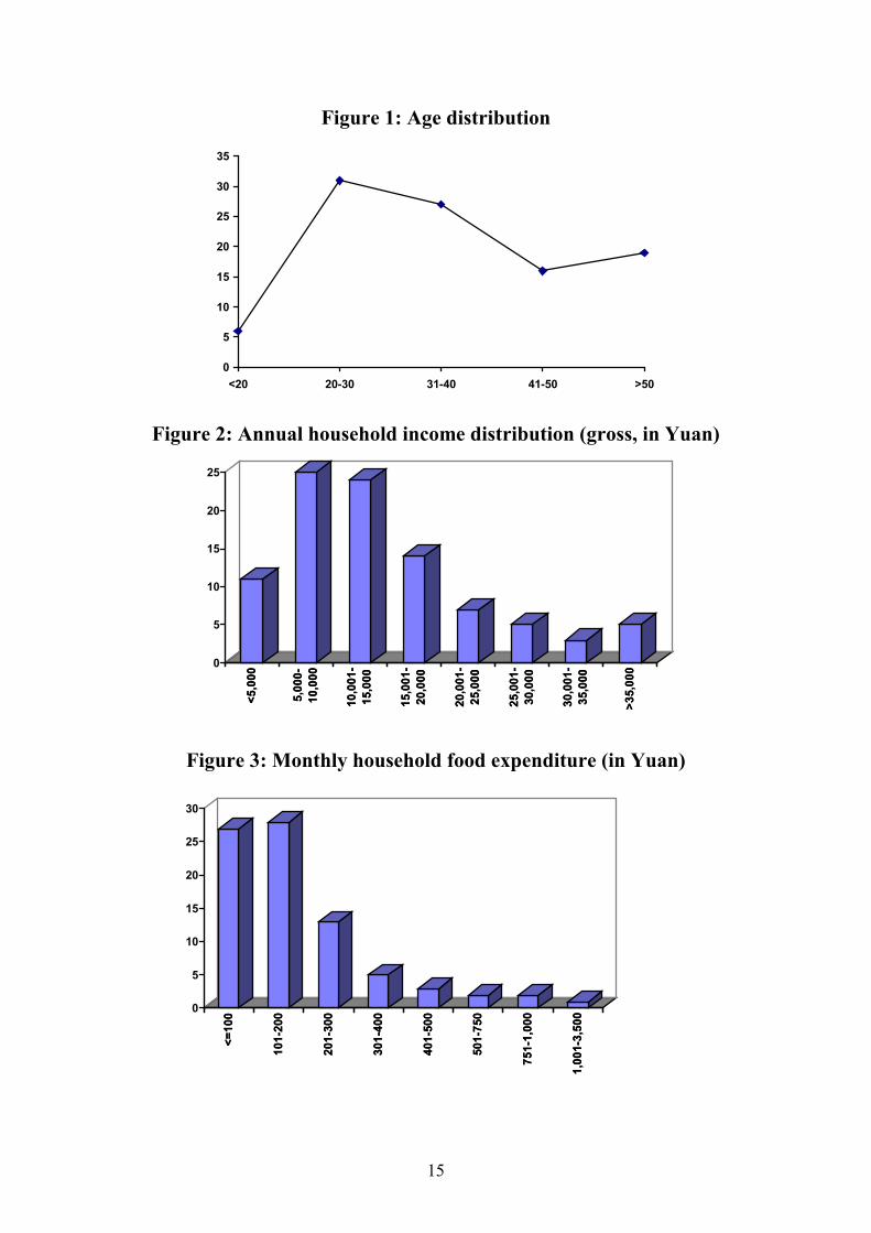
5.1. Socio-economic characteristics Table 2 presents a summary of socio-economic variables. 61% of the sample are males. The age distribution is wide, as depicted in Figure 1, with an average age of 37. Three quarters of respondents are married or living with a partner and almost all the remaining are single. The average family size is 3.8 with a median of 3. As expected, the mean number of children below 16 in each household is low at 0.7, with a median of 1. The majority of respondents reached secondary education (42%) or a professional degree (21%); a fifth has university education; only 2% have no education at all. In clear contrast to what typically happens in many developed countries surveys, the income non-response was very low, at only 3%. The average household gross income per year is 14,160 Yuan, with the median being 12,500 Yuan. Figure 2 shows the distribution of income. In spite of the sampling difficulties encountered, the surveyed population’s income spans through a considerable range. The mean monthly food expenditure is 205 Yuan (with a median of 150 Yuan). As depicted in Figure 3, food expenditure across households ranges widely from 20 to 3,500. Aggregating over a year, mean food expenditure is found to constitute on average about a fifth of household’s gross income. Most respondents are employed full-time, with only 2% of unemployed people, 2% of housewives, 5% of students and 11% of retired people (Table 2). Taking care of the home full-time does not seem to be a common occupation in Beijing as all family members seem to typically work outside the home. A number of variables were included as proxies for household wealth. These include possession of a car and of various household appliances. The results are also in Table 2. Cars are a luxury good with only 6% of respondents owning one. Other luxury items are cloth and dish washing machines, owned by only 3% of the surveyed population each. In contrast, owning a TV is almost universal and the large majority of respondents also has access to a refrigerator (77%) and a tape/CD player (70%). However, less than half the sample has a telephone or an indoor bathing facility. Table 3 presents the correlations between income, food expenditure and wealth proxies. As expected, all the correlations are positive with the highest

13

associations being found between income and (i) having a telephone (0.40), (ii) food expenditure (0.38) and (iii) having access to an indoor bathing facility (0.36). These results suggest that household income seems to captures well the economic well-being of the surveyed population. Further analysis showed that there were no significant differences between sub-samples that were administered different versions of the questionnaire.

14

Table 2: Summary statistics of selected socio-economic variables

Variables

Total number of individuals 999

Demographic variables

Males 61%

Age (mean) 37

Married / living w/ partner 73%

Family size (mean) 3.82

Number of children (mean) 0.69

Education: No Education 2%

Primary 12%

Secondary 42%

Professional degree 21%

University 19%

Economic variables

Yearly household income (mean, gross, in Yuans) 14,160

Income non-response 3%

Employment: Self-employed 17%

Farmer 13%

Employed full-time 41%

Unemployed 2%

Looking after the home full time 2%

Student 5%

Retired 11%

Monthly household food expenditure (mean, in Yuans) 205

Car 6%

Home appliances: TV 91%

Washing machine 3%

Refrigerator 77%

Indoor bathing facilities 46%

Tape/CD player 70%

Telephone 47%

Dishwasher 3%

15

Figure 1: Age distribution

0

5

10

15

20

25

30

35

<20 20-30 31-40 41-50 >50

Figure 2: Annual household income distribution (gross, in Yuan)

<5,0

00

5,00

0-10

,000

10,0

01-

15,0

00

15,0

01-

20,0

00

20,0

01-

25,0

00

25,0

01-

30,0

00

30,0

01-

35,0

00

>35,

0000

5

10

15

20

25

<5,0

00

5,00

0-10

,000

10,0

01-

15,0

00

15,0

01-

20,0

00

20,0

01-

25,0

00

25,0

01-

30,0

00

30,0

01-

35,0

00

>35,

000

Figure 3: Monthly household food expenditure (in Yuan)

<=10

0

101-

200

201-

300

301-

400

401-

500

501-

750

751-

1,00

0

1,00

1-3,

5000

5

10

15

20

25

30

<=10

0

101-

200

201-

300

301-

400

401-

500

501-

750

751-

1,00

0

1,00

1-3,

500

16

5.2. Attitudinal and behavioural questions The preliminary section of the survey contained a considerable number of attitudinal and behavioural questions, which were intended to make respondents explore their personal thoughts on environmental issues in general and river water quality in particular, as a preparation for responding to the valuation question. In addition, these questions were designed to reveal as much as possible about the underlying motives for supporting river preservation, so as to aid in the interpretation of the valuation responses. A number of questions exploring respondents use of rivers, perceptions and knowledge of river water pollution were also included.

5.2.i General environmental attitudinal questions The opening attitudinal question asked respondents about the degree of importance of several general problems. Table 4 summarises the results. Somehow surprisingly, nearly a quarter of the sample ranked environmental problems as the most important problems in the Beijing area, out of a list that included a range of 8 different problems (poverty, health, education, urban security, inflation, environment, transport and unemployment). Sometimes, results such as these are upward biased and derive from letting respondents know what the primary focus of the survey is; however, this is unlikely the

Table 3: Correlation between household income and other proxies for household wealth

Proxies Income

Monthly food expenditure 0.38

Car 0.25

TV set 0.13

Cloth washing machine 0.27

Refrigerator 0.31

Indoor bathing facility 0.36

Tape / CD player 0.25

Telephone 0.40

Dish washing machine 0.18

17

case, as the question was the first of the interview. Urban security was the second most mentioned problem, followed by education and transport. Another question followed about the relative importance of a number of particular environmental problems (species extinction, waste management, drinking water pollution, air pollution, sanitation, soil erosion, destruction of forests, water pollution in lakes and rivers). Air pollution was considered by 25% of the sample to be the most important environmental concern (Table 4). Water pollution of lakes and rivers came in the 4th place, mentioned by 16% of respondents, close behind waste management and drinking water pollution.

Given the focus of the survey, a large number of attitudinal questions were posed specifically with respect to river water quality, where respondents were asked to express their agreement or disagreement with a series of statements. These were mainly aimed at understanding how the Chinese view their rivers, uncovering the most important consequences of river water pollution and assessing the motivations behind conservation attitudes. Figure 4 below presents the results for these attitudinal questions. Statement 4a reflects an anthropocentric view of river pollution, that is, river preservation is important only in so much as it affects human activities. The results show that the large majority of respondents does not support this outlook, with 86% disagreeing or strongly disagreeing with it and less than 10% agreeing.

Table 4: Most important problems in the Beijing Region

Problems % Most Important Problems in the Beijing Region

Environmental Problems 23

Urban Security 18

Public Education Quality 13

Transport 12

Most Important Environmental Problems in the Beijing Region

Air Pollution 25

Waste Management 18

Drinking Water Pollution 17

Water Pollution in Lakes and Rivers 16

Sanitation 13

18

Statement 4b provides an indication of the importance of selfish use-related motivations when evaluating river preservation. The large rate of disagreement with this statement (83%) shows that respondents are not drawn primarily from selfish individual use motives when evaluating the importance of river pollution, that is, they support river protection even though they may not use the river. 71% of the surveyed population agreed or strongly agreed with statement 4c indicating that indirect use motivations are important determinants of supporting river preservationnew business in a particular area can boost the local economy and indirectly benefit a number of people. Statement 4d reflects what is known in the economic literature as an ‘option value’, i.e. independent of their present use of a river, a person may support river preservation so that he or she can benefit from it in the future, if so desired. As shown in the figure, 81% of the sample agreed with the statement and only 7% disagreed, indicating the importance of this type of motivation. The next statement, 4e, is a translation of a ‘bequest motive’, that is, wanting to preserve rivers for the benefit of future generations. The results show that there was a strong tendency to identify with this motivation from 88% of the sample. Statements 4f and 4g relate to ‘existence values’, that is, supporting river preservation for the sake of the ecosystems, animals and plants that rivers provide the habitat for, irrespective of any personal spin-offs they may generate. Statement 4f met with agreement from over 80% of the sample while statement 4gmore stringent as it mentions preservation at all costswas still supported by a majority of 63%. This result highlights the importance of altruistic motivations in the Chinese population while considering river preservation. Statements 4h and 4i were constructed to reflect trade-offs between clean-up costs and water quality benefits and between job creation and river pollution, respectively. A majority of 68% rejects the viewpoint that rivers should be kept clean only if the costs are not very highalthough a substantial minority of 20% agrees with it. In addition, 77% disagree that is worth having a factory that provides jobs but pollutes a river. In both accounts, environmental concerns seem to be rated high, when compared to economic factors. Finally, statement 4j puts river pollution into a more general context, by establishing a comparison between fish deaths and other important problems. As shown in Figure 4j, this question split the sample roughly in half48% identified with the view that there are more important things to worry about, while 35% rejected it. This is consistent with the fact that river pollution only came 4th when evaluated against other environmental concerns (Table 4).

19

20

Figure 4: Attitudes towards rivers

a. “If no one uses a river, the fact that it is polluted is not important”

Strongly Disagree

Disagree

Neither Agree norDisagree

Agree

Strongly Agree

32 %

54 %

5 %

7 %

1 %

0 10 20 30 40 50 60

Strongly Disagree

Disagree


Agree

Strongly Agree

b. “If a river becomes polluted, the fact that other people will not be able to use it for recreation does not bother me if I, myself, don’t use it”

Strongly Disagree

Disagree


Agree

Strongly Agree

25 %

58 %

9 %

6 %

2 %

0 10 20 30 40 50 60

Strongly Disagree

Disagree


Agree

Strongly Agree

21

c. “It is worth spending more money on water quality in rivers because clean

rivers attract new business to the area”

Strongly Disagree

Disagree

Neither Agree nor Disagree

Agree

Strongly Agree

2 %

6 %

21 %

56 %

15 %

0 10 20 30 40 50 60

Strongly Disagree

Disagree


Agree

Strongly Agree

d. “Even if I don’t use rivers at the moment I would still like to preserve them in case I want to use them in the future, even if that costs me money now”

Strongly Disagree

Disagree


Agree

Strongly Agree

2 %

5 %

12 %

64 %

17 %

0 10 20 30 40 50 60 70

Strongly Disagree

Disagree


Agree

Strongly Agree

22

e. “We have a responsibility to protect rivers for future generations, even if

that costs us money”

Strongly Disagree

Disagree


Agree

Strongly Agree

2 %

5 %

5 %

65 %

23 %

0 10 20 30 40 50 60 70

Strongly Disagree

Disagree


Agree

Strongly Agree

f. “The fact that some animals and plants may die due to pollution in rivers is a serious problem”

Strongly Disagree

Disagree


Agree

Strongly Agree

2 %

6 %

11 %

60 %

21 %

0 10 20 30 40 50 60

Strongly Disagree

Disagree


Agree

Strongly Agree

23

g. “If the animals and plants that live in a river are unique than the river

should be protected at all costs”

Strongly Disagree

Disagree


Agree

Strongly Agree

3 %

14 %

20 %

45 %

18 %

0 5 10 15 20 25 30 35 40 45

Strongly Disagree

Disagree


Agree

Strongly Agree

h. “Rivers should only be kept clean if the costs are not very high, otherwise we will just have to learn to live with polluted rivers”

Strongly Disagree

Disagree


Agree

Strongly Agree

19 %

49 %

11 %

19 %

2 %

0 5 10 15 20 25 30 35 40 45 50

Strongly Disagree

Disagree


Agree

Strongly Agree

24

i. “If a factory pollutes a river but provides many jobs then it is worth having the factory”

Strongly Disagree

Disagree


Agree

Strongly Agree

25 %

52 %

10 %

11 %

2 %

0 10 20 30 40 50 60

Strongly Disagree

Disagree


Agree

Strongly Agree

j. “We have more important things to worry about than some dead fish in a polluted river”

Strongly Disagree

Disagree


Agree

Strongly Agree

6 %

29 %

17 %

38 %

10 %

0 5 10 15 20 25 30 35 40

Strongly Disagree

Disagree


Agree

Strongly Agree

It is interesting to assess to what extent the different motivations reflected in these attitudinal statements overlap at the level of the individual respondent. Table 5 reports the correlation coefficients between each pair of attitudinal variables depicted in Figure 4, and reveals a number of interesting points.

25

• There are particularly strong positive correlations between people motivated by non-use values (existence, bequest and option values). For example, the correlation between those motivated by bequest and option values is 0.45; indeed, 79% of the sample consistently either agreed or disagreed with both of these statements.

• The correlations are also high and positive between non-use and indirect use values. For example, the correlation between people motivated by option concerns and indirect use values is 0.37.

• Similarly, there is a significant positive correlation (0.37) between those motivated by selfish concerns and those motivated by anthropocentric values. Indeed, 79% of the sample consistently agreed or disagreed with both of these statements.

• The two statements concerning trade-offs were expressed in a negative fashion, i.e. disagreement with the statements implies a strong support of river protection while agreement indicates that other concerns (like monetary costs or job creation) are considered to be more important. Hence, the correlations found between the trade-off statements and the ‘selfish’ and ‘anthropocentric’ variables are positive as expected.

Table 5: Correlation between different motives for supporting river preservation

selfis

h anthrop trade

-off 1trade-off 2

indirect option bequest exist 1 exist 2

selfish 1

anthrop 0.37 1

trade-off 1 0.33 0.32 1

trade-off 2 0.40 0.38 0.41 1

indirect -0.21 -0.20 -0.16 -0.22 1

option -0.27 -0.24 -0.20 -0.24 0.37 1

bequest -0.28 -0.28 -0.18 -0.23 0.32 0.45 1

existence 1 -0.26 -0.26 -0.27 -0.24 0.36 0.40 0.28 1

existence 2 -0.23 -0.27 -0.20 -0.24 0.33 0.28 0.20 0.37 1

Note: ‘selfish’ concerns are represented by the statement in Fig. 4b, ‘anthropocentric’ by 4a, ‘trade-off 1’ by 4h, ‘trade-off 2’ by 4i, ‘indirect’ by 4c, ‘option’ by 4d, ‘bequest’ by 4e, ‘existence 1’ by 4f and ‘existence 2’ by 4g.

26

• There is a negative correlation between those motivated mainly by selfish and anthropocentric motivations and those who are primarily driven by non-use and altruistic concerns. For example, the correlation between the ‘bequest’ and either of the ‘selfish’ and ‘anthropocentric’ variables is -0.28.

• None of the correlations reported are particularly high in absolute terms (although most are statistically significant).

From Figure 4 and Table 5, the following conclusions can be made:

• There seem to be two distinct types of respondents: a majority that is mainly driven by altruistic motivations, not related to a direct use of the resource (i.e., bequest and existence concerns, indirect use values and option values) and a small minority that is motivated primarily by more ‘selfish’ considerations related to a personal use of the resource.

• No single motivation stands out as the most important factor driving respondents attitudes, regardless of respondent type. There are significant positive correlations between a number of motivations, indicating that many considerations play a role in individual attitudes.

• People seem to be very consistent in answering sometime difficult attitudinal questions, i.e. most of those driven by selfish motivations are not also driven by altruistic concerns, a result which would lead us to disbelief the entire exercise.

• By and large, these results conform to prior expectations regarding the motivations behind support of river protection, in light of the pilot results and of previous findings reported elsewhere in the literature: non-use values seem to play a fundamental role in explaining people’s attitudes towards the preservation of river water quality. This study shows that this result also extends to developing countries.

5.2.ii Characterisation of behaviour The importance of non-use and indirect use values in the evaluation of river water pollution was assessed in the previously discussed group of questions. To complete the analysis, an assessment and characterisation of the recreational use of rivers by the target population was needed. The questions described below provide this information. Table 6 reports frequencies of visits to any river in the Beijing area and to the two target rivers, the Chaobai and the Nan Sha He. A relatively large percentage of the surveyed population (24%) visits a river on a daily basis,

27

while 17% do so once or twice a week. Only 8% claims to never visit a river. These results can be explained by the sampling frame that was used. As will be discussed in Section 6.2.iv below, there was some over-sampling of rural populations and of villages located next to rivers; hence, it is not surprising that the frequency of visits to rivers is so high. Note that many people pass through a river location in transit to other areas and this also counted as a ‘visit’. The frequency of visits to the two target rivers was naturally much lower, with only 5% and 9% of respondents making daily visits to the Chaobai and the Nan Sha He, respectively (Table 6). In the case of the Chaobai, 17% of the sample visits once a year at most and 55% never go there; the Nan Sha He is even less visited with 59% never visiting and 10% visiting once a year or less often. The people who were interviewed on site at the Chaobai or the Nan Sha He were also asked for details of their travel. These are reported in Table 7. The most common means of transportation were walking and using a bicycle. This indicates that many of the visitors are locals. The average journey time was 30 minutes (with a median of 10 minutes). Considering both on and off-site respondents, when visiting a river, a large proportion of people usually travel alone (27%) which is consistent with the fact that many people may stop at a river while in transit to other locations. 19% travel with family (with children) and with adult friends, respectively (Table 7).

Table 6: Frequency of visits to rivers in the Beijing area (%)

Visit Frequency All Rivers

Chaobai

Nan Sha He

Daily 24 5 9

3 to 6 times a week 8 2 4

Once or twice a week 17 5 6

Every 2 weeks 7 2 2

Every month 9 3 2

A few times a year 14 9 5

Once a year or less often 11 17 10

Never 8 55 59

28

All respondents, whether interviewed on or off-site, were asked what sort of activities they engaged in while visiting a river. The results are presented in Table 8. The most popular activities are off-stream uses like ‘walking’ and ‘relaxing and enjoying the scenery’, mentioned by 54% and 45% of respondents, respectively. About a fifth of the sample also mentioned ‘to let children play in or around the river’; arguably, this particular use of the river could enhance bequest concerns. In stream activities like swimming, fishing, boating and sailing were also mentioned respectively by 20%, 18%, 17% and 3% of respondents (Table 8). Although very few respondents considered species extinction to be an important issue in the opening attitudinal questions, 11% did mention ‘watching wildlife’ as an activity. Many of these activities are done simultaneously. Therefore, the fact that many people mention ‘walking’ as an activity does not necessarily mean that ‘walking’ is the main reason why they visit a river. Nonetheless, when inquired about the one most important reason for taking a trip to a river, the same pattern of results emerge: ‘walking’ is still the most important activity for 29% of the people, followed by ‘relaxing and enjoying the scenery’ for 11%. Off-stream activities seem to be predominant in the Beijing rivers. Finally, and in accordance to what was suggested earlier on, the results show that more than a third of the sample (35%) make a trip to a river while on transit to somewhere else (Table 8). This is consistent with the high rate of daily visits

Table 7: Travel details

Travel details

Methods of Transport

Walked all the way 25%

Bicycle 20%

Journey time (min)

Mean 30

Median 10

Companions

Alone 27%

In family with children 19%

With adult friends 19%

29

(Table 6) and the percentage of people travelling alone reported before (Table 7).

Table 8: River activities

River Activities %

Walking 54

Relaxing and enjoying scenery 45

In transit 35

To let children play in or around river 21

Swimming for pleasure 20

Fishing for pleasure 18

Boating or canoeing 17

Watching wildlife 11

Picnicking 9

Never use 8

Washing or cleaning yourself or your clothes 6

Visiting a cafe/restaurant for a drink/meal 3

Sailing or sailboarding 3

Note: people may do more than one activity

5.2.iii Perceptions of river water quality Apart from the type of motivation behind supporting river preservation, perceptions about current river water quality standards and about sources of pollution may affect people’s evaluation and WTP for programmes to reduce river pollution. This section presents results from questions eliciting people’s perceptions: (i) about pollution levels in Beijing rivers in general, and in the Chaobai and Nan Sha He, in particular (for those familiar with these rivers only); and (ii) about pollution sources. Perceptions of water quality were assessed through a series of statements that respondents were asked to agree or disagree upon. Figure 5 depicts the results. A number of important findings emerge:

30

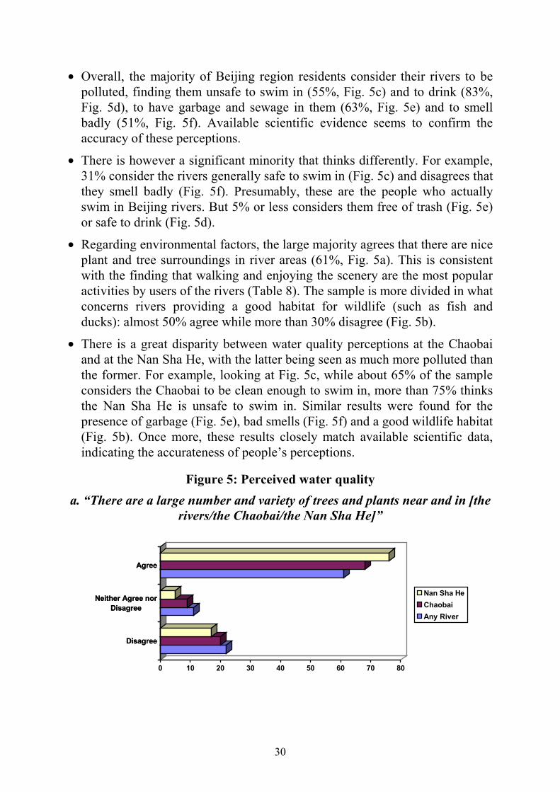
• Overall, the majority of Beijing region residents consider their rivers to be polluted, finding them unsafe to swim in (55%, Fig. 5c) and to drink (83%, Fig. 5d), to have garbage and sewage in them (63%, Fig. 5e) and to smell badly (51%, Fig. 5f). Available scientific evidence seems to confirm the accuracy of these perceptions.

• There is however a significant minority that thinks differently. For example, 31% consider the rivers generally safe to swim in (Fig. 5c) and disagrees that they smell badly (Fig. 5f). Presumably, these are the people who actually swim in Beijing rivers. But 5% or less considers them free of trash (Fig. 5e) or safe to drink (Fig. 5d).

• Regarding environmental factors, the large majority agrees that there are nice plant and tree surroundings in river areas (61%, Fig. 5a). This is consistent with the finding that walking and enjoying the scenery are the most popular activities by users of the rivers (Table 8). The sample is more divided in what concerns rivers providing a good habitat for wildlife (such as fish and ducks): almost 50% agree while more than 30% disagree (Fig. 5b).

• There is a great disparity between water quality perceptions at the Chaobai and at the Nan Sha He, with the latter being seen as much more polluted than the former. For example, looking at Fig. 5c, while about 65% of the sample considers the Chaobai to be clean enough to swim in, more than 75% thinks the Nan Sha He is unsafe to swim in. Similar results were found for the presence of garbage (Fig. 5e), bad smells (Fig. 5f) and a good wildlife habitat (Fig. 5b). Once more, these results closely match available scientific data, indicating the accurateness of people’s perceptions.

Figure 5: Perceived water quality a. “There are a large number and variety of trees and plants near and in [the

rivers/the Chaobai/the Nan Sha He]”

Disagree


Agree

0 10 20 30 40 50 60 70 80

Disagree


Agree

Nan Sha HeChaobaiAny River

31

b. “[The rivers/the Chaobai/the Nan Sha He] are a good habitat for wildlife, e.g. fish, ducks”

Disagree


Agree

0 10 20 30 40 50 60 70

Disagree


Agree


c. “The water in [the rivers/the Chaobai/the Nan Sha He] is clean and safe for humans to swim in”

Disagree


Agree

0 10 20 30 40 50 60 70 80

Disagree


Agree


d. “The water in [the rivers/the Chaobai/the Nan Sha He] is clean and safe for humans to drink”

Disagree


Agree

0 10 20 30 40 50 60 70 80 90 100

Disagree


Agree


32

e. “[The rivers/the Chaobai/the Nan Sha He] do not have much trash and sewage in them”

Disagree


Agree

0 10 20 30 40 50 60 70 80

Disagree


Agree


f. “[The rivers/the Chaobai/the Nan Sha He] do not smell badly”

Disagree


Agree

0 10 20 30 40 50 60 70

Disagree


Agree


These results could have important implications for the WTP for the Chaobai, the Nan Sha He and for rivers in general. For example, respondents may be willing to pay more to prevent further deterioration of water quality in rivers that they perceive as being already quite polluted; or conversely, they could be willing to pay more to prevent cleaner rivers from becoming polluted. However, while water quality perceptions may conceptually matter, the available empirical evidence suggests that this is not the case, at least for Beijing area residents. As mentioned above , the original survey design that was pre-tested aimed at eliciting the WTP for a number of different scenarios where not only the scalethe number of rivers affected but also the scopethe degree of pollutionof the injury changed. Respondents were found to be able to differentiate between scale effectsi.e. the WTP for one

33

river was significantly lower than the WTP for all riversbut not between scope effects—i.e. the answers were insensitive to the level of damage specified, in terms of a water quality ladder. These results could be interpreted as indicative of either ill-defined preferences over a range of damage levels, or true indifference between these levels. The damage levels presented in the pre-test were not in fact very different from each other, as they aimed to represent realistic changes in water quality (e.g. changes from level C to level B or from level C to level A in the water quality ladder, where the difference between B and A regards the potential to drink the water). Hence, in the light of the pilot results indicating insensitivity to the degree of water pollution, the prior expectation is that, ceteris paribus, different water quality perceptions in the Chaobai and the Nan Sha He will not translate into different WTP amounts. The next section will present further evidence on this matter. The questionnaire also elicited responses on the perceived sources of pollution. As depicted in Table 9, industry (60%) is considered to be the main source of river pollution. From what data exists, this seems to be an accurate description of reality. Domestic sewerage and trash are seen as the second and third pollution sources. It is interesting to note that sewerage comes before trash (although only by 1%) in spite of the fact that garbage floating in the water and lying in river banks is normally more visible though less noxious than untreated sewerage discharges.

5.2.iv Attitudes towards the scenario and the questionnaire The questionnaire included some follow-up attitudinal questions to evaluate respondents attitudes towards the proposed programme that they were being asked to pay for, and towards the questionnaire in general.

Table 9: Perceived sources of pollution

Pollution sources % Discharge from industrial sources 60

Sewage from villages and towns 12

Dumping of trash from villages and towns 11

Dumping of factory waste 3

Seepage from agriculture 2

34

By and large, as shown in Table 10, the attitudes towards the proposed programme were highly favourable with a large majority of respondents thinking it would receive strong public support, would attain the desired results and could be implemented successfully by the government. As expected, only the payment mechanism (higher taxes and prices) received disparate comments, with roughly half the sample considering it a bad method of funding the clean-up programme and the other half considering it good (very similar results had already been found in the pilot). Typically, the percentage of those disproving of the payment mechanism is even higher, for example, very few people would say that a tax increase is a good idea; the fact that there wasn’t a clear-cut payment vehicle in this case, but a general increase in taxes and prices, probably reduced the potential hostility rate.

Note: people may agree with more than one statement

Finally, the last question of the survey asked respondents for their overall views on the questionnaire. As illustrated in Figure 6, the survey instrument seemed to work quite well in the field with the majority of respondents (56%) considering it to be interesting and only a minority thinking it was too long (18%), boring (9%) or not credible (%).

Figure 6: Attitudes towards the questionnaire

Boring

Not credible

Difficult

Too long

Interesting

2 %

9 %

9 %

18 %

56 %

0 10 20 30 40 50 60

Boring

Not credible

Difficult

Too long

Interesting

Table 10: Attitudes towards the proposed programme to preserve river water quality

Statements % Agree “The programme will receive strong public support” 88

“The government is capable of implementing the programme” 79

“The programme will attain the desired results” 70

“Higher taxes and prices are a good way of funding the programme” 42

35

6 Results: Contingent Valuation Questions

6.1 The Valuation Questions

6.1.i Scenarios and policies Contingent Valuation questions begin with the outlining of a scenario. The scenario provides the respondent with a clear description of the ‘good’ he is going to be asked to value. Following the scenario the respondent is presented with a policy or project that will be undertaken to ensure that the respondent receives the ‘good’. The policy description will also include the description of a payment vehicle, through which the respondent will be expected to pay for the policy. Good contingent valuation design involves creating realistic and uncomplex scenarios and policies that can be clearly understood by respondents. Following the pretest the survey was comprehensively redesigned. As described previously in Section 4.2, the pilot revealed a number of important points that aided in this design:

• There was a general awareness of pollution in the Chaobai River, though a significant proportion (40%) perceived the water quality as being at a level that did not deter recreational activities.

• The pretest questionnaire consisted of three different versions which had been designed to assess whether respondents could distinguish between differences in the proposed scope of water quality changes in the Chaobai River (Version A involved improvement to a medium water quality, Version B involved improvement to a high water quality) and differences in the scale of these changes (Version C involved an improvement to a medium water quality in ALL the rivers around Beijing). Econometric tests suggested that respondents’ WTP was not significantly different in respect to scope but was with respect to scale.

• Nearly 90% of respondents replied that they understood the payment vehicle (a general rise in taxes and prices), though only 50% were convinced that this was a good way to fund water quality improvements. Indeed, of those stating a zero WTP nearly 20% stated that their reason for doing so was that they believed their taxes were already too high.

The design of the main survey scenario, therefore, had to accommodate the fact that, at present, a considerable number of river users did not consider the rivers too polluted. Also, the pretest suggested that varying the scope of water quality improvements would not significantly change WTP. A further complication was introduced when the main survey was expanded from just the Chaobai

36

River to include the Nan She He, on which no data on perceived pollution existed. The scenario then had to establish clear and realistic endpoints for the valuation of changing river water quality. This was achieved through the use of a map and showcards. First, the respondent was shown a map of the area around Beijing. The major rivers on the map were highlighted in yellow and the two focus rivers were highlighted in green. The respondent was familiarised with the map and the geographical area over which the scenario would be relevant was established. Second, the respondent was shown SHOWCARD 1, which bore pictures and symbols describing reasonably unpolluted rivers in which most forms of recreation were possible. The showcard was a reasonable reflection of the perceived pollution levels reported in the pretest. The respondent was informed that this showcard represented the current quality of water in rivers around Beijing. The respondent was then presented with SHOWCARD 2, that bore pictures and symbols describing highly polluted rivers in which most forms of recreation were inadvisable. The respondent was informed that due to increasing pollution over the next five years, water quality in either one or all of the rivers highlighted on the map would decline from that described in the first showcard to that shown in the second showcard. The scenario, therefore established clear endpoints that would be common across all rivers. For reasons that shall be elaborated later, two different scenarios were designed:

• The water quality in ALL the rivers in the Beijing area deteriorate

• The water quality ONLY in the Nan She He would deteriorate whilst the water quality in the other rivers remained at its present level

The results of the pretest were also important in designing the policies presented in the final survey. First, the pretest had revealed that WTP was not significantly influenced by the scope of the policy. In other words, it was likely that trying to identify a difference in WTP in a clean up to a medium level compared to a high level of water quality was likely to be unfruitful. On the other hand, since the pre-test had given encouraging results concerning respondent’s abilities to distinguish different scales of water quality improvements, the main survey concentrated on splitting the sample to assess WTP for single river improvements compared to all river improvements. The policy, therefore, used in the final survey was the implementation of a series of projects to control the pollution coming from communities and industries along the rivers such that water quality would not decline over the

37

next five years but remain at its present level. Three versions of the policy were designed:

• Pollution control measures installed along ALL rivers

• Pollution control measures installed ONLY along the Nan She He

• Pollution control measures installed ONLY along the Chaobai Despite the difficulties encountered in the pretest with the payment vehicle, this was not changed due to a lack of credible alternatives. People who refused to pay anything towards the proposed policies were, therefore, questioned to identify those who had a genuine WTP of zero and those who simply objected to the form in which they had to pay for the policy. Table 11 depicts the combinations of scenarios and polices that were used in forming the four questions used in the survey. These four questions were asked to different samples such that the WTP figures resulting could be compared without fear of bias.

Table 11: Valuation questions, policies and scenarios

Question Number Scenario Policy

1 ALL rivers deteriorate

Maintain water Quality in ALL rivers


Maintain water Quality in Nan Sha He

3 ONLY Nan Sha He deteriorates



Maintain water Quality in Chaobai

Table 12: Combinations of scenarios and polices Maintain River

Quality in ALL Rivers

Maintain River Quality ONLY in the

Nan She He

Maintain River Quality ONLY in

the Chaobai River water quality in ALL rivers deteriorates

QUESTION 1 QUESTION 2 QUESTION 4

38

River water quality in only the Nan She He deteriorates

QUESTION 3

Why were these particular combinations of scenarios and policies chosen? Table 12 depicts the same information as Table 11 but within a policy-scenario matrix. For the purposes of research, the WTP derived from the four valuation questions are only directly comparable if they lie in the same column or row of the matrix. That is, so long as we hold the scenario constant between two valuation questions we can judge the influence of altering the policy and vice versa. What then might we expect to detect from our experimental set-up? Well, the four questions derived from the scenario-policy matrix have been designed to investigate a number of different issues, primarily how scale and the existent of substitute rivers might influence WTP. Clearly, our prior expectations are that the highest WTP figures will be returned for Question 1 in which the most extensive scenario, ALL rivers deteriorating, is combined with the most extensive policy, ALL rivers maintained at their present quality. Certainly, it is expected that Question 1 would return higher WTP figures than those returned from Questions 2 and 4, where only the Nan Sha He or the Chaobai were maintained at present water quality. A priori, it is impossible to predict whether the WTP to maintain water quality only in the Nan Sha He would be higher or lower than WTP to maintain water quality only in the Chaobai. It was expected that any difference in WTP for maintained water quality in these two rivers would depend, to a large extent, on the degree to which they were used for recreation by the population of the Beijing Metropolitan Area. A key factor in determining WTP for a single river improvement would be the degree to which individuals use that particular river due to its exclusive recreational qualities. If the substitution possibilities are high then people can easily switch their recreation activities to another river. In such a case, we would not expect the decline in water quality in one river to elicit a large WTP response. In Questions 2 and 4 the possibility of such substitution effects is precluded since it is made clear to the respondent that the water quality of ALL the rivers in the Beijing Metropolitan Area will decline. To test for the possibility that such substitution possibilities might exist, Question 3 was included. In this scenario all rivers in the region remain available for recreation activities. Individuals are asked to state how much they would pay solely to maintain the water quality in the Nan Sha He. If substitution possibilities exist, which they clearly do, then we would expect the

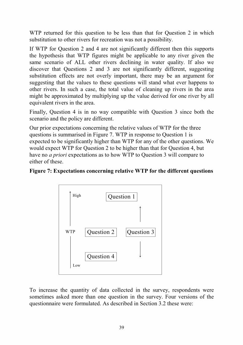
39

WTP returned for this question to be less than that for Question 2 in which substitution to other rivers for recreation was not a possibility. If WTP for Question 2 and 4 are not significantly different then this supports the hypothesis that WTP figures might be applicable to any river given the same scenario of ALL other rivers declining in water quality. If also we discover that Questions 2 and 3 are not significantly different, suggesting substitution effects are not overly important, there may be an argument for suggesting that the values to these questions will stand what ever happens to other rivers. In such a case, the total value of cleaning up rivers in the area might be approximated by multiplying up the value derived for one river by all equivalent rivers in the area. Finally, Question 4 is in no way compatible with Question 3 since both the scenario and the policy are different. Our prior expectations concerning the relative values of WTP for the three questions is summarised in Figure 7. WTP in response to Question 1 is expected to be significantly higher than WTP for any of the other questions. We would expect WTP for Question 2 to be higher than that for Question 4, but have no a priori expectations as to how WTP to Question 3 will compare to either of these. Figure 7: Expectations concerning relative WTP for the different questions

WTP

Question 1

Question 2

Question 4

Question 3

High

Low

To increase the quantity of data collected in the survey, respondents were sometimes asked more than one question in the survey. Four versions of the questionnaire were formulated. As described in Section 3.2 these were:

40

• VERSION 1: Scenario: ALL rivers in the Beijing Region deteriorate. QUESTION 4 : WTP to maintain the quality of water ONLY in Chaobai. QUESTION 1: WTP to maintain the quality of water in ALL rivers.

• VERSION 2: Scenario: ALL rivers in the Beijing Region deteriorate. QUESTION 2: WTP to maintain the quality of water ONLY in Nan Sha He. QUESTION 1: WTP to maintain the quality of water in ALL rivers.

• VERSION 3: (reverse of Version 2) Scenario: ALL rivers in the Beijing Region deteriorate. QUESTION 1: WTP to maintain the quality of water in ALL rivers. QUESTION 2: WTP to maintain the quality of water ONLY in Nan Sha He

• VERSION 4: Scenario: ONLY the Nan Sha He deteriorates. QUESTION 3: WTP to maintain the quality of water ONLY in the Nan Sha He.

The use of two questions in the different versions of the questionnaire allowed us to test one further aspect of contingent valuation questionnaire design, namely whether question order influenced respondents WTP. For example, it is possible to test whether those answering Question 1 second in a sequence of questions (i.e. those responding to Versions 1 and 2) report a consistently different WTP to those answering this question first (i.e. those responding to Version 3).

6.1.ii The Valuation Questions Having presented a scenario and policy the respondent was then faced by a set of valuation questions. First, the respondent was asked a Referendum Question, and provided the response to this was yes, was then faced by a WTP Question. The Referendum Question simply asked whether the respondent would be WTP anything for the proposed policy. This type of question elicits a response of

41

either ‘YES I would pay something for this policy’ or ‘NO I would not pay anything for this policy’. If respondents answered no to the referendum question then they were asked to give their reasons. Some reasons for answering no were considered protest votes rather than a genuine WTP of zero. For example, if a respondent declared that their reason for voting no was because:

• they did not believe in the scenario that had been presented, or

• they objected to having to pay money for maintaining water quality in rivers, then these responses had to be discarded from the data set. On the other hand, alternative reasons including:

• not having enough money to pay for river water quality maintenance, or

• not believing that maintaining river water quality was of sufficient importance to warrant paying any money,

were assumed to reflect a genuine WTP of zero. Those who answered yes to the referendum question were then presented with the WTP Questions. These were presented in the so-called double bounded dichotomous choice format. In recent years, the dichotomous choice (DC) format, where respondents are faced with a predetermined take it or leave it price (known as a bid level) for the good being valued, has become the method of choice in most CV applications (NOAA, 1993). It is generally accepted that respondents are better able to answer questions of this type as they more closely resemble the choices faced in normal markets. The problem with asking just one DC question is that it requires very large sample sizes to obtain statistically significant results. A partial solution to this problem is to adopt the double-bounded dichotomous choice (DBDC) approach used in this study. Here the initial DC question is supplemented with a follow-up question in which an initial yes (no) is followed-up with a subsequent willingness to pay amount higher (lower) than the first bid level. This format gives significantly more information on the underlying WTP (Hanemann et al., 1991). The actual amounts used as bid levels were defined with reference to the open-ended WTP responses given in the pre-test. Only 3% of respondents had stated a WTP of over 500 Yuan so this was taken as the highest bid. However, and maybe due to cultural factors not detected in the pre-test stages, the final dataset contained a large number of ‘Yes’ responses even to the highest bid level. This has caused some problems with the analysis of the data, as described in Section 6.4.i.

42

The logical flow through the valuation section of the questionnaire is presented in Figure 8.

Figure 8: Logical flow of valuation section

SCENARIO Respondent presented with scenario describing

declining water quality in all or one of the rivers in the Beijing Region

POLICY A policy is described that will ensure water quality is maintained in all or one of the rivers in the Beijing

Region

REFERENDUM QUESTION The respondent is asked whether they are

WTP anything for the proposed policy

NO YE

INITIAL BID LEVELThe respondent is presented with a monetary amount (the initial bid level) and asked

whether they are WTP to pay this amount

NO VOTE REASONS The respondent is asked to provide a reason for not wanting to pay for the policy. Those with a genuine WTP

of zero can therefore be distinguished from those simply protesting against the scenario or

policy

LOW BID LEVEL The respondent is presented

with a second, lower monetary amount (the low bid level) and asked whether they are WTP

to pay this amount

HIGH BID LEVEL The respondent is presented

with a second, higher monetary amount (the high bid level) and asked whether they are WTP to

pay this amount

END OF VALUATION QUESTION

YENO

43

6.2. Sampling and Weighting

6.2.i Theory of sampling and weighting Carrying out econometric analysis on data collected in a survey relies on the fact that the survey sample is representative of the population from which it is drawn. Surveys carried out by professional survey companies select their samples in advance by defining a so-called sampling strategy. That is they divide the population up in to a series of strata based, for example, on age, income and sex, and ensure that the proportions of people in their sample coming from each of the defined strata is the same as the proportions found in the general population. Unfortunately, such a procedure was not possible with the China survey for a number of reasons:

• the added complexities of survey administration with sampling quotas were deemed too complex to be reasonably carried out by the survey team

• data on the population distribution of certain important stratifying variables were not known when the survey was being designed

• data on the population distribution of certain important stratifying variables could only be estimated from data returned from the survey

Fortunately, another approach to achieving a representative sample is available. First, the researcher must define a sampling strategy based on characteristics that he believes to be important to WTP for the policy. Next he identifies the proportions of the population falling into the strata defined by the sampling strategy. By dividing these values by the proportions of the sample falling in the same strata the researcher defines a weight for each observation in the dataset. As shall be shown later, this weight can be used in econometric analysis to adjust the data so it behaves like a representative sample. In effect, the weight reduces the importance of observations from households with characteristics that have been oversampled and increases the importance of observations from households that have characteristics that were undersampled.

6.2.ii The sampled population Before a sampling strategy could be defined, a clearly defined population had to be identified from which this sample could be drawn. The population from which we decided to sample had to fulfil, as best as possible, three criteria:

• It had to comprise as best as possible the population within which households might express a positive WTP for the rivers defined in the scenarios outlined above.

44

• It had to coincide with regions for which population data were available. The Beijing Metropolitan Region is divided into four urban districts, four suburban districts and ten rural counties for which population data were available from the 1995 census

• It had to represent an area from which it was practical to sample Taking these criteria into account, the population was defined as those households living in the following areas:

• the three rural counties that surround the Chaobai and Nan Sha He rivers in which the RUWEP projects are being applied: Tong Xian, Chang Ping and Shun Yi

• the four suburban districts: Chao Yang, Hai Dian, Shi Jing Shan, Feng Tai

• the four urban districts: Xi Cheng, Dong Cheng, Xuan Wu, Chong Wen These districts and counties covered most of the geographic area that was in reasonable proximity to the two rivers that formed the focus of the study. The map used in the survey was designed to cover nearly the entire area defined by these regions.

6.2.iii Sampling locations Interviews were undertaken in two major rural towns Tong Xian and Shun Yi, a large variety of smaller rural settlements including Nan She and Xiao Pu, the site of the RUWEP engineering project. Interviews were also undertaken in suburban districts, including Hai Dian and Qing He and some 150 interviews were conducted in various neighbourhoods in all four of the urban districts. To ensure that an adequate number of users of the rivers were contained in the sample, two onsite samples were taken. These consisted of 200 surveys along the banks of the Chaobai and a further 300 along the banks of the Nan Sha He.

6.2.iv Sampling Strategy, Population and Sample Characteristics The sampling strategy devised after the survey had been completed, was based on three characteristics. These were;

• Whether a household came from an urban, suburban or rural region which it was hoped would reflect differences in social outlooks on the benefits of water quality improvements in rivers

• Whether the household was above or below average income for the type of region they came from which it was hoped would reflect differences in economic influences on WTP for water quality improvements

45

• Whether the household visited a river or rivers frequently, occasionally or never, which was required to compensate for the sampling of on-site users of rivers

The sampling strategy, therefore, defined eighteen sample strata. Defining population proportions for those living in the different regions was relatively easy since this data was published in the Statistical Year Book of Beijing 1996. Dividing these strata according to income is also a simple task since half the population in each of these regions must be above the average income and half must be below. The frequency of visits to a river or rivers strata was extrapolated from the data. It was assumed that there would be no systematic bias in the distribution of this variable for those that were sampled off site. It was also assumed that this distribution did not vary across regions or income. The proportions of the off site sample making frequent/occasional/no visits to any river/the Nan She He/the Chaobai were used as the population proportions for this variable. The final population proportions in the various strata are given in Table 15 at the end of this section. The calculation of the sample proportions for the subsamples facing each of the four questions also required some data manipulation. First the region of origin had to be identified for each respondent. This was a relatively easy, though arduous task. Each respondent had been asked to mark where they lived on a map stapled to the back of the questionnaire. By examining each of these maps and locating each respondent in an urban, suburban or rural category, it was possible to calculate the proportions of each subsample from the different types of region. Mean income for each region type was taken from the Statistical Year Book of Beijing 1996. Using figures for inflation and growth the 1995 figures (given in the Year Book) were extrapolated to the beginning of 1997. Each household was identified as being above or below this value for their region and the subsample proportion calculated accordingly. The distribution of frequency of visits to either All rivers, the Nan She He or the Chaobai in the subsamples was taken straight from the questionnaire. Some simple analysis of the data reveal that the interviewing strategy failed to return a random sample from the defined population. Table 13 compares the population distribution between urban, suburban and rural districts with that sampled in the study. Clearly, the study sample had oversampled from the Rural population and undersampled from the Urban and Suburban ones.

46

Similarly, the interviewing of on-site visitors clearly biased the sample towards households frequently recreating at the study rivers. Table 14 illustrates this fact for visitation rates to the Nan Sha He. Only 9% of those interviewed in off-site locations claimed to visit the Nan Sha He frequently (i.e. once a month or more often) compared to 20% in the entire sample. Likewise, over three-quarters of the off-site sample stated that they never visited the Nan Sha He compared to a figure of 61% in the entire sample. Again, the sample was clearly biased towards frequent users.

Given the major differences between the sample’s and the true population’s characteristics. It was likely that weighting would significantly improve the accuracy of the results The weights used in the econometric analysis to rebalance each of the four sub-samples are shown in Table 16.

Table 13: Comparison of population distribution between urban, suburban and rural districts compared to that sampled in the study

Region Population: Sample:

Households Percentage Households Percentage

Urban 870,000 32% 139 16%

Suburban 1,290,000 48% 253 29%

Rural 534,000 20% 467 54%

Total 2,694,000 100% 859 100%

Table 14: Frequency of Visits to the Nan Sha He

Frequency of Use Off Site All Sample

Frequent 9% 20%

Occasional 14% 17%

Never 76% 61%

Total 100% 100%

47

Tab

le 1

5: P

opul

atio

n pr

opor

tions

use

d in

wei

ghtin

g

POPU

LATI

ON

ALL

RIV

ERS

N

AN

SH

A H

E

CH

AO

BA

I

UR

BA

N

UR

BA

N

UR

BA

N

Vis

itatio

n

Vis

itatio

n

Vis

itatio

n

Inco

me

Nev

er

Infr

eque

nt

Freq

uent

Inco

me

Nev

er

Infr

eque

nt

Freq

uent

Inco

me

Nev

er

Infr

eque

nt

Freq

uent

Bel

ow A

vg

1%

7%

7%

B

elow

Avg

13

%

2%

0%

B

elow

Avg

11

%

4%

0%

Abo

ve A

vg

1%

7%

7%

A

bove

Avg

13

%

2%

0%

A

bove

Avg

11

%

4%

0%

SUB

UR

BA

N

SU

BU

RB

AN

SUB

UR

BA

N

V

isita

tion

V

isita

tion

V

isita

tion

Inco

me

Nev

er

Infr

eque

nt

Freq

uent

Inco

me

Nev

er

Infr

eque

nt

Freq

uent

Inco

me

Nev

er

Infr

eque

nt

Freq

uent

Bel

ow A

vg

4%

12%

9%

Bel

ow A

vg

16%

6%

2%

Bel

ow A

vg

17%

7%

0%

Abo

ve A

vg

4%

12%

9%

Abo

ve A

vg

16%

6%

2%

Abo

ve A

vg

17%

7%

0%

RU

RA

L

R

UR

AL

RU

RA

L

V

isita

tion

V

isita

tion

V

isita

tion

Inco

me

Nev

er

Infr

eque

nt

Freq

uent

Inco

me

Nev

er

Infr

eque

nt

Freq

uent

Inco

me

Nev

er

Infr

eque

nt

Freq

uent

Bel

ow A

vg

2%

3%

5%

B

elow

Avg

7%

1%

1%

Bel

ow A

vg

4%

3%

2%

Abo

ve A

vg

2%

3%

5%

A

bove

Avg

7%

1%

1%

Abo

ve A

vg

4%

3%

2%

48

Tab

le 1

6: W

eigh

ts u

sed

in e

cono

met

ric

anal

ysis

SAM

PLE

WEI

GH

TS

ALL

RIV

ERS

NA

N S

HA

HE

1

NA

N S

HA

HE

2

CH

AO

BA

I

UR

BA

N

V

isita

tion

V

isita

tion

Vis

itatio

n

V

isita

tion

Inco

me

Nev

er

Infr

eque

nt

Freq

uent

In

com

e N

ever

In

freq

uent

Fr

eque

ntIn

com

e N

ever

In

freq

uent

Freq

uent

Inco

me

Nev

er

Infr

eque

ntFr

eque

nt

Bel

ow A

vg

4.03

3.

20

3.33

B

elow

Avg

2.26

4.

58

Uns

mpl

dB

elow

Avg

2.

24

0.72

U

nsm

pld

Bel

ow A

vgU

nsm

pld

6.34

U

nsm

pld

Abo

ve A

vg

1.34

2.

44

2.00

A

bove

Avg

1.68

1.

31

Uns

mpl

dA

bove

Avg

1.

64

0.72

0.

00

Abo

ve A

vgU

nsm

pld

3.17

0.

23

SUB

UR

BA

N

V

isita

tion

V

isita

tion

Vis

itatio

n

V

isita

tion

Inco

me

Nev

er

Infr

eque

nt

Freq

uent

Inco

me

Nev

er

Infr

eque

nt

Freq

uent

Inco

me

Nev

er

Infr

eque

ntFr

eque

nt

Inco

me

Nev

er

Infr

eque

ntFr

eque

nt

Bel

ow A

vg

2.85

2.

29

1.52

B

elow

Avg

1.71

1.

32

0.86

B

elow

Avg

1.

43

1.02

0.

14

Bel

ow A

vgU

nsm

pld

5.85

0.

58

Abo

ve A

vg

5.71

2.

37

2.12

A

bove

Avg

2.26

1.

49

1.43

A

bove

Avg

2.

14

1.13

0.

24

Abo

ve A

vgU

nsm

pld

2.93

0.

58

RU

RA

L

Vis

itatio

n

Vis

itatio

n

V

isita

tion

Vis

itatio

n

Inco

me

Nev

er

Infr

eque

nt

Freq

uent

Inco

me

Nev

er

Infr

eque

nt

Freq

uent

Inco

me

Nev

er

Infr

eque

ntFr

eque

nt

Inco

me

Nev

er

Infr

eque

ntFr

eque

nt

Bel

ow A

vg

0.48

0.

28

0.27

B

elow

Avg

0.64

0.

14

0.12

B

elow

Avg

0.

84

0.38

0.

50

Bel

ow A

vg6.

54

0.26

0.

09

Abo

ve A

vg

0.61

0.

32

0.22

A

bove

Avg

0.77

0.

19

0.10

A

bove

Avg

0.

84

0.75

0.

63

Abo

ve A

vg3.

27

0.21

0.

06

49

6.3. Econometric Analysis

6.3.i Introduction In this section we describe how the data collected from the contingent valuation surveys was analysed and present some of the results of this analysis. The analysis used ‘cutting edge’ econometric techniques of not inconsiderable complexity and some readers may wish to skip certain sections of this chapter. As a brief overview, the econometric analysis of contingent valuation surveys seeks to build a model that explains why respondents answer WTP questions as they do. The model uses responses from the survey to judge exactly how different factors, such as income or frequency of use of a river, influence a households WTP for water quality in a river. As described in the first section the model is built up from our understanding of how WTP is distributed in the population. The model used to describe this distribution consists of two parts; one explaining whether people are WTP anything for water quality in rivers (the spike model) and the other explaining how much those who are WTP something are prepared to pay (the WTP model). These two models are explained in the third and fourth sections of this chapter. In the fourth section the two models are combined to present one whole behavioural model. In the final section the full model is estimated using the data from the questionnaire and the results of this estimation are presented. The econometric model describing how decisions concerning WTP are made can be used to estimate the average WTP in the population. The estimation of average WTP is the subject of the next chapter.

6.3.ii The Population Distribution of WTP Figure 9 presents a graph of the distribution of WTP amongst respondents to the open-ended valuation question asked in the pre-test. Though both the scenario and policy presented in the pre-test were somewhat different from that used in the main survey, there is every reason to expect that respondents to the main survey would show a very similar distribution of WTP. Indeed the pattern of WTP depicted in the graph is one regularly witnessed in WTP studies. The first thing to note about this distribution is that, not surprisingly, no one has declared a WTP less than zero - no one believes they should be paid money to have the water quality in rivers improved. Conversely, a fair number of respondents are clearly not WTP anything for river water quality improvements and account for the large spike in the distribution at zero. For those respondents expressing a positive WTP, the majority return reasonably low values around 100 Yuan or less, whilst a steadily decreasing number of households are

50

prepared to pay larger amounts. In statistical parlance the distribution of those with a positive WTP appears to be skewed to the right.

Figure 9: Distribution of WTP amongst respondents to pre-test survey

0

5

10

15

20

25

-50 0 50 100 150 200 250 300 350 400 450 500 550 600

No. of households in the sample expressing this WTP

WTP (Yuan)

When data is collected using the open-ended valuation question format, the calculation of the average WTP in the population is easy. It is simply the average WTP expressed by the sample (given, of course, that this is a representative sample). For reasons outlined above, data in the main survey was collected using the dichotomous choice question format. In the dichotomous choice framework, the models researchers use to derive average WTP depend on making certain assumptions concerning the underlying shape of the distribution of WTP. Figure 10 depicts three theoretical distributions that might be of use to researchers in modelling WTP. The spike distribution is the most easily defended. This corresponds quite clearly with the point mass at zero WTP shown in Figure 9. It defines that portion of the population that are not WTP anything towards the proposed policy. Our model will have to include an element that will predict the height of this spike. In other words, we will want the model to ascertain what fraction of the population have a WTP of zero, and what fraction of the population have a positive WTP. So, what about the distribution of WTP amongst those who are WTP for the policy? Figure 10 plots two other theoretical distributions that might be used by the researcher to describe the underlying pattern of positive WTP. The first, the normal distribution, has been used in many studies and has a number of advantages, notably in the simplicity with which models using this distribution

51

can be analysed and average WTP figures calculated. It also has a number of drawbacks. First, the normal distribution is symmetric, it shows none of the pattern of right skewedness that we observed in the WTP responses to the pre-test questionnaire. Second, the normal distribution is not necessarily truncated at zero. Assuming the normal distribution could lead to a model that predicted a portion of the population having negative WTP.

Figure 10: Possible theoretical distributions of WTP

So, what about the distribution of WTP amongst those who are WTP for the policy? Figure 10 plots two other theoretical distributions that might be used by the researcher to describe the underlying pattern of positive WTP. The first, the normal distribution, has been used in many studies and has a number of advantages, notably in the simplicity with which models using this distribution can be analysed and average WTP figures calculated. It also has a number of drawbacks. First, the normal distribution is symmetric, it shows none of the pattern of right skewedness that we observed in the WTP responses to the pre-test questionnaire. Second, the normal distribution is not necessarily truncated at zero. Assuming the normal distribution could lead to a model that predicted a portion of the population having negative WTP. For these reasons the log-normal distribution would appear to be a much closer approximation to the true underlying distribution of WTP. This distribution is skewed to the right and doesn’t allow for WTP below zero and is clearly a better approximation to the pattern revealed in Figure 9. Fortunately, as shall be described in a later section, it is possible to use an econometric trick known as the Box-Cox transformation to test whether the

Spike Distribution

Log-Normal Distribution

Normal Distribution

No. of households in the population expressing this WTP

WTP 0

52

best approximation to the underlying distribution is normal, log-normal or, for that matter, a whole array of similarly shaped distributions (Box and Cox, 1964).

6.3.iii The Referendum Question and the Spike Model The first step in building a full econometric model describing WTP for river water quality in the Beijing region is to model the spike distribution (see Hanemann and Kristöm, 1995). That is, we want to create a model that will predict whether a particular household will have either a WTP of zero or some positive WTP. Clearly, this is a binary decision. Responses to the referendum question provide the relevant data on whether a particular household has declared a zero WTP or a positive WTP. To model data of this type economists begin by assuming that there exists some underlying, unobservable latent variable, let us call this wi (where the i subscript denotes household i). We can think of this latent variable as a utility index that is determined by certain variables including the characteristics of the household. If wi exceeds some threshold level wi* then the household will declare a positive WTP. Since, it does not matter what absolute value wi takes, the threshold value can be normalised to 0. Hence, for household i

WTP = 0 if wi < 0 (1)

WTP > 0 if wi ≥ 0

Of course, the researcher does not know the value of wi for a household, he can only make a prediction (let us call this vi), based on the variables he thinks might be influential to its value (let us label these as the vector Xs, where the s subscript refers to the fact that these are variables used in modelling the spike distribution). Thus,

wi = vi(Xsi, βs) + ei (2)

where βs represents a vector of parameters that measure the influence of the Xsi variables on the value of vi, and

ei represents the element of the latent variable that the researcher is unable to predict. Since the researcher does not know the value of ei he must regard it as a random element. Thus the true value of wi could lie above or below the researcher’s prediction (vi). If we assume that the random element follows some known probability distribution, it becomes possible to predict, for any given value of vi, the probability that wi will lie above the threshold level, wi*. In more formal terms, we can replace Equation (2) in Equation (1) giving,

53

WTP = 0 if vi + ei < 0 (3)

WTP > 0 if vi + ei ≥ 0

and, since we know the probability distribution of ei we can rearrange equation (3) to give,

Pr(WTP = 0) = Pr(ei < -vi) (4)

Pr(WTP > 0) = Pr(ei ≥ -vi)

Put simply, our estimate of the utility index, vi, can take either a positive value or a negative value. If vi is negative then it lies below the threshold at which a household will declare a positive WTP. Only values of ei that are more positive than vi is negative would result in a value for the true utility index (wi) that was above the threshold. Thus, the probability of having a positive WTP is the probability that the random element, ei will take on a value that is more positive than the estimated utility index , vi, is negative (note the double negative that would occur in Equation (4) from negative values of vi). A similar argument can be made for positive values of vi.

For a number of good reasons, it is usually assumed that the random element follows a standard normal distribution1. Since the normal distribution is symmetric, we reach the convenient conclusion that the probability of ei taking a value greater than a certain number is identical to the probability that it will take a value less than the negative of that number. Hence, we can derive the following expression,

Pr(WTP = 0) = Pr(ei > vi) (5)

= 1 - Φ(vi) = 1 - p

Pr(WTP > 0) = Pr(ei ≤ vi)

= Φ(vi) = p

where Φ is the cumulative standard normal distribution, and p is the probability that WTP is greater than zero. The spike model is illustrated in Figure 11. Clearly if the value of vi is high (as it is for household 1) then the probability that wi lies above the threshold value

1 This assumption concerning the distribution of ei results in an econometric model that is known generally in econometrics as the probit model. We can think of our spike model as being a specific application of the probit model to describe the spike distribution in WTP responses.

54

is also high since only unusually low values of the random element, ei, could reduce the value of wi below the threshold level. Conversely for a low value of vi (as shown for household 2) the probability of the true latent variable, wi, lying above the threshold value is relatively small.

Figure 11: The spike model

How do we go about estimating such a model? The first step is to parameterise vi. That is we construct an equation that describes how various variables (such as a household’s income or the frequency with which they visit rivers) might influence the value of the latent variable. One simple parameterisation is:

vi = βs0 + βs1Xs1i + βs2Xs2i + ... + βsnXsni (6)

So, given our first estimates of the values for the βs parameters, it is possible to calculate a value of vi for all of the households in the sample. Then using the model described in equation (5), we can calculate the total probability that the households in the sample would have answered the referendum question as they did, according to

( )L p pid

id

i

i i= − −∏ ( )1 1 (7)

where di is a dummy variable which equals 1 if the respondent answered yes to the referendum question and 0 if the respondent answered no, and

0 (w*) v1 = Xs1βs

p = 0.5

p2 = 0.2

p = 1

p1 = 0.9

+∞ -∞ v2 = Xs2βs

Probability of wi lying above zero

Cumulative standard normal distribution (ΦΦΦΦ)

(distribution of -ei)

55

L is known as the likelihood function and measures the total probability (predicted by the model at the given parameters) that respondents will have answered the referendum question in the way they did.

For convenience it is more usual to work with the log of this expression

( )log log ( ) log( )L d p d pi

i i i i= + − −� 1 1 (8)

Using computer maximisation routines, the model is estimated by selecting the set of parameters, βs, that maximise this log likelihood expression. These values for βs give the best estimates of how the Xs variables influence a household’s response to the referendum question. For now we shall leave the model of the spike distribution and concentrate on how we go about modelling those households with a positive WTP

6.3.iv The Double-Bounded Dichotomous Choice Question and the WTP Model

Similar to the referendum question, the double-bounded dichotomous choice (DBDC) question, returns data in a binary format. Indeed the econometric model used to analyse this data is very similar to that just discussed for the referendum question. In modelling the referendum question data we constructed a latent variable or utility index that was used to gauge the likelihood of a household expressing a WTP greater than zero. In analysing the DBDC data, however, we are no longer dealing with an unobservable utility index but a WTP function whose value will be used to gauge the likelihood that a household will accept a particular bid level. One important difference between the two models, therefore, is that where the absolute value of the utility index was not important, the absolute value of the WTP function is essential. Similar to the true latent variable wi used for the referendum question we can begin by stating that each household has a true WTP for the policy being offered in the valuation question. Let us represent this true WTP as yi. As with wi, the researcher does not directly observe yi. In the DBDC questions the respondent is presented with a threshold value (the equivalent of wi*) in the form of a bid level. Let us represent these by bi for the initial bid level, bl for the lower bid level and bu for the upper bid level. Thus in response to each question the respondent will answer,

Yes if yi ≥ b (9)

56

and No if yi < b

Of course, the researcher does not know the value of yi, but uses an econometric model to estimate a prediction of this true value. Let us call this estimated WTP function zi. zi is described as a function because we expect its value to be influenced by a number of variables (let us label this vector Xw, where the w subscript refers to the fact that these are variables used in modelling the WTP distribution). Thus,

yi = zi(Xwi, βw) + εi (10)

where βw represents a vector of parameters that measure the influence of the Xwi variables on the value of zi, and

εi represents the part of the true WTP that the researcher is unable to predict.

Again, we treat εi as a random element, but since the absolute value of the WTP function, zi, is important, we cannot simply assume that it follows a standard normal distribution. Instead εi is modelled as coming from a normal distribution with a mean of zero and a variance of σ, a parameter that we will have to estimate. Replacing equation (10) in equation (9) results in the respondent answering,

Yes if zi + εi ≥ b (11)

and No if zi + εi < b

Since we know the probability distribution of εi we can rearrange equation (11) to give,

Pr(Yes) = Pr(εi ≥ b - zi) (12)

Pr(No) = Pr(εi < b - zi)

To return to a standard normal distribution, we can account for the variance in the random element εi by dividing both sides of the inequality in equation (12) by σ. Hence, the probability of a household being WTP a given bid level can be modelled by,

Pr(Yes) = 1 - Φ((b - zi)/σ) (13)

Pr(No) = Φ((b - zi)/σ)

Of course in the DBDC question format, households are faced by not just one bid level, but two, such that those answering:

57

• Yes, Yes have a WTP that is higher than the upper bid level bu

• Yes, No have a WTP higher than the initial bid level, bi, and lower than bu

• No, Yes have a WTP lower than bi, but higher than the lower bid level, bl

• No, No have a WTP below bl Expanding equation (13) to take account of this added information gives,

Pr(Yes, Yes) = 1 - Φ((bu - zi)/σ) (14)

Pr(Yes, No) = Φ((bu - zi)/σ) - Φ((bi - zi)/σ)

Pr(No, Yes) = Φ((bi - zi)/σ) - Φ((bi - zi)/σ)

Pr(No, No) = Φ((bl - zi)/σ)

The probabilities defined in equation (14) represent the intervals illustrated in Figure 12.

Figure 12: The Double Bounded Dichotomous Choice Model

Again it is possible to parameterise zi

zi = βw0 + βw1Xw1i + βw2Xw2i + ... + βwnXwni (15)

The model described in Equation (14) rests on the assumption that the underlying population distribution of WTP follows a normal distribution. However, as described above, there is good reason to believe that WTP is more likely to follow a log-normal distribution. The log normal distribution would

bi b +∞ -∞ bl

Probability of zi being

greater than b

Cumulative standard normal distribution (ΦΦΦΦ)

(distribution of εεεεi)

YN

YY

NY

NN

58

result from assuming that the WTP function (Equation (10)) is log-linear in form such that,

log(yi) = zi(Xwi, βw) + εi (16)

Thus, the normal distribution model can be transformed into a log-normal model simply by taking the log of the bid levels (b) in Equation (14). Of course, by imposing this transformation on the data, we are making an a priori assumption concerning the underlying distribution of WTP. However, using a useful transformation of the WTP function known as the Box-Cox transformation (Box and Cox, 1964), it is possible to allow the data to dictate what is the most appropriate distributional assumption. The Box-Cox transformation is as follows,

( )y z Xii wi w i

λ

λβ ε−

= +1 , (17)

where λ is the Box-Cox parameter that will be estimated in the model

Notice that if λ takes on a value of 1 then the model simply collapses back to the straight linear model of Equation (10). If, however, λ takes on a value of zero then the model will result in the log-linear model of Equation (16). Thus, the value of the λ parameter will provide us with a test of whether WTP is best represented by the linear or log-linear form and hence whether the underlying distribution of WTP is normal or log-normal. Once again, the WTP model is estimated using maximum likelihood techniques. Combining the expressions in Equation (14) and adding the Box-Cox transformation we can build up the log likelihood function,

( )

( ) ( )

( ) ( )

log log ,

log , ,

log , ,

L yy b z Xi

yn b z X b z X

ny b z X b z X

ui wi w

ui wi w

ii wi w

ii wi w

li wi w

= −−

−�

��

�

��

�

��

�

��

�

��

�

��

�

�

+−

−�

��

�

��

�

��

�

�� −

−−

�

��

�

��

�

��

�

��

�

��

�

��

+−

−�

��

�

��

�

��

�

�� −

−−

�

��

�

��

�

� 11

1 1

1 1

Φ

Φ Φ

Φ Φ

λ

λ λ

λ λ

λβ σ

λβ σ

λβ σ

λβ σ

λβ σ

( )

��

�

��

�

��

�

��

+−

−�

��

�

��

�

��

�

��

�

��

�

��

�

��

nn b z Xli wi wlog ,Φ

λ

λβ σ1

(18)

59

where yy is a dummy variable taking on the value 1 if the respondent answered yes to both WTP questions and the value 0 otherwise, and

yn is a dummy variable taking on the value 1 if the respondent answered yes to the first question and no to the second question, and the value 0 otherwise, and

ny is a dummy variable taking on the value 1 if the respondent answered no to the first question and yes to the second question, and the value 0 otherwise, and

nn is a dummy variable taking on the value 1 if the respondent answered no to both WTP questions, and the value 0 otherwise.

The model estimates the λ, σ and βw parameters. The parameter estimates are those that result in it being most likely that the households in the sample would have responded to the WTP questions in the way they did.

6.3.v Adding Weights and the Full Maximum Likelihood Function As we shall see shortly, the model describing responses to the Referendum question and that describing responses to the WTP questions can be easily combined into one full log likelihood function. One thing remains, however, to complete the model. That is the observation weights discussed above. In the full likelihood function, the importance of each observation is adjusted to account for the fact that the sample may have over- or under-sampled from certain strata of the population. This process of weighting is termed weighted exogenous sample maximum likelihood (Manski and Lerman, 1977). The final likelihood function developed for the purposes of analysing this survey data was as follows:

60

[ ( )( )( )

( )

( ) ( )

( )

log log ,

log ,

log , ,

log ,

L w di

v X

yy b z X

yn b z X b z X

ny b z X b z X

i i i si s

ui wi w

ui wi w

ii wi w

ii wi w

li

= −

+ − − −�

��

�

��

�

��

�

��

�

��

�

��

+−

−�

��

�

��

�

��

�

�� −

−−

�

��

�

��

�

��

�

��

�

��

�

��

+ − −�

��

�

��

�

��

�

�� − − −

� 1

1 1

1 1

1 1

Φ

Φ

Φ Φ

Φ Φ

β

λβ σ

λβ σ

λβ σ

λβ σ

λ

λ

λ λ

λ λ

( )

( )

( ) ( )( )]

wi w

li wi w

i i si s

nn b z X

d v X

,

log ,

log ,

β σ

λβ σ

β

λ

�

��

�

��

�

��

�

��

�

��

�

��

+−

−�

��

�

��

�

��

�

��

�

��

�

��

+ −

Φ

Φ

1

1 (19) where wi is the observation weight defined as the fraction of the sample in the

respondent’s sampling strata divided by the fraction of the population in that strata

The final model estimating the λ, σ and βw and βs parameters was written in Intercooled STATA 5.0, an econometric package for Statistics and Data Analysis, published by the Stata Corporation, using the supplied maximisation routine.

61

6.3.vi Estimation of the Model and Regression Results The econometric model described in the previous section was estimated with the data collected in the survey (a process known as regression). In this section the estimates of the parameters of the model are presented. First, a simplified model was estimated that investigated the best fitting distribution for WTP function. Given information gathered from these preliminary model estimations, the final model was formulated and estimated.

Table 17 reports the result of the preliminary regressions. The model estimated corresponds to that described by Equation (18) in which the Box-Cox transformation is included. The estimated value of the Box-Cox parameter (λ), will allow us to assess the correct transformation of the WTP function. For simplicity both the Referendum and WTP functions were included in their most basic form containing just a constant and no regressors (Xs, Xw).

Table 17: Tables reporting regression results with Box-Cox Transformation Question 1: All Rivers Number of observations: 557 Log Likelihood: -831.89

Coefficient Standard Error z-statistic

Referendum Model: Constant 1.09 .07 16.4***

WTP Model: Constant 6.54 1.47 4.5***

σ 1.83 .69 2.6***

λ .08 .08 1.0

62

Question 2: Nan She He, all rivers deteriorate Number of observations: 396 Log Likelihood: -582.04


Referendum Model: Constant .59 .07 8.8***


σ 1.07 .56 1.9*

λ -.02 .11 -0.2 Question 3: Nan She He, other rivers do not deteriorate Number of observations: 196 Log Likelihood: -283.81




σ 1.12 .68 1.65*

λ -.004 .13 -0.03

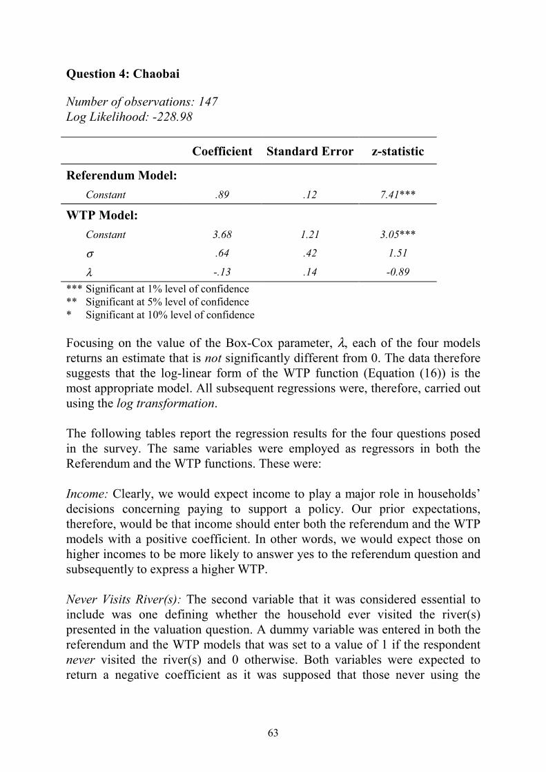
63

Question 4: Chaobai Number of observations: 147 Log Likelihood: -228.98




σ .64 .42 1.51

λ -.13 .14 -0.89 *** Significant at 1% level of confidence ** Significant at 5% level of confidence * Significant at 10% level of confidence Focusing on the value of the Box-Cox parameter, λ, each of the four models returns an estimate that is not significantly different from 0. The data therefore suggests that the log-linear form of the WTP function (Equation (16)) is the most appropriate model. All subsequent regressions were, therefore, carried out using the log transformation. The following tables report the regression results for the four questions posed in the survey. The same variables were employed as regressors in both the Referendum and the WTP functions. These were: Income: Clearly, we would expect income to play a major role in households’ decisions concerning paying to support a policy. Our prior expectations, therefore, would be that income should enter both the referendum and the WTP models with a positive coefficient. In other words, we would expect those on higher incomes to be more likely to answer yes to the referendum question and subsequently to express a higher WTP. Never Visits River(s): The second variable that it was considered essential to include was one defining whether the household ever visited the river(s) presented in the valuation question. A dummy variable was entered in both the referendum and the WTP models that was set to a value of 1 if the respondent never visited the river(s) and 0 otherwise. Both variables were expected to return a negative coefficient as it was supposed that those never using the

64

river(s) would be less likely to want to pay for maintaining water quality and also have a lower positive WTP. Question: For Question 1 and Question 2, a final variable was included in both parts of the model. This was another dummy variable, set to a value of 0 if this was the first of the two valuation questions the respondent answered and 1 if it was the second. A number of WTP studies, in which more than one valuation question has been posed in the same questionnaire, have reported what are termed order effects (Carson and Mitchell, 1995; Halvorsen, 1996). In other words, households’ responses are systematically biased by whether they answer a particular valuation question first or second in a sequence of such questions. There were no a priori reason to suppose this variable would take on either a positive or a negative coefficient. Table 18: Tables reporting full regression results Question 1: All Rivers Number of observations: 557


Referendum Model:

Constant 0.79 .15 5.4***

Income .00005 .00001 4.2***

Never Visits Rivers

-.49 .23 -2.2**

Question -.27 .14 -1.9*

WTP Model: Constant 4.77 .12 40.3***

Income .00005 8.3e-06 6.3***

Never Visits Rivers

-.09 .25 -0.4

Question -.26 .13 -2.0**

σ 1.17 .06 19.3***

65

Question 2: Nan She He, all rivers deteriorate Number of observations: 396


Referendum Model:

Constant .29 .18 1.6

Income .00005 .00001 4.5***

Never Visits the Nan She He

-.11 .16 -0.7

Question -.09 .14 -0.6


Income .00004 9.5e-06 4.5***


-.37 .17 -2.2**

Question .48 .16 3.1***

σ 1.09 .07 14.6*** Question 3: Nan She He, other rivers do not deteriorate Number of observations: 196


Referendum Model:

Constant .60 .24 2.5**

Income .00002 .00001 1.4


.02 .23 0.1


Income .00002 .00001 1.8*

Never Visits the Nan She He -.05 .25 -0.2

σ 1.15 .10 11.2***

66

Question 4: Chaobai Number of observations: 147


Referendum Model:

Constant .82 .18 4.5***

Income .00004 .00002 1.6

Never Visit the Chaobai

-.85 .32 -2.6***


Income .00001 .00002 0.7

Never Visits the Chaobai

-.38 .39 -1.0

σ 1.14 .11 10.5*** *** Significant at 1% level of confidence ** Significant at 5% level of confidence * Significant at 10% level of confidence

Broadly speaking the regression results conform to our prior expectations: Income: Income enters both the Referendum and WTP models with a positive coefficient in response to all four questions. In more cases than not the coefficient is also highly significant. Never visit river or rivers: Also, in general, the dummy variable for never visiting a river or rivers is, as expected, negative in sign and for the most part a significant explanatory variable. Question order: As for the variable reflecting the respondent answering this question second in a sequence of valuation questions, it would appear that question order has negligible effect on respondent’s likelihood of responding yes to the Referendum Question. However, it is clear that those answering Question 1 as a second valuation question return a significantly lower WTP than those that answer this question first. Whilst, those answering Question 2 as a second valuation question return a significantly higher WTP. The cause of this phenomena can probably be explained through examining the order in which respondents answered the valuation questions.

67

The question order in the four versions of the questionnaire was described in Section 6.1.i. Those answering Question 1 (maintained water quality in all rivers) as a second valuation question were responding to either Version 1 or Version 2 of the questionnaire. In both cases they had been asked to express their WTP for a less extensive policy (maintained water quality in just one river) in the first valuation question. The regression results suggest that respondents’ replies to the valuation questions are biased downwards if they have valued a less extensive policy before a more extensive policy. The reverse also appears to be true. Those answering Question 2 (maintained water quality only in the Nan She He) as a second valuation question were responding to Version 3 of the questionnaire. In this case they had been asked to value a more extensive policy in the first valuation question (maintained water quality in all rivers). The regression results, in this case, show respondents’ replies to be biased upwards if they had been asked to value a more extensive policy first. This sort of bias is frequently termed anchoring in the contingent valuation literature. The idea behind ‘anchoring’ being that respondents’ answers are tied to an earlier answer they have given. Thus, if a respondent values all rivers first then his responses to a second question concerning just one river will likely be biased upwards, whereas a respondent valuing one river first will likely return lower values to a subsequent question concerning all rivers. As we shall see in the next section it is possible to correct for this anchoring bias when deriving WTP figures from the regressions.

68

6.4. Willingness to Pay

6.4.i Calculation of WTP How then is total WTP derived from the regression analysis presented in the last section? Essentially, there are two steps. First a figure representing a measure of the ‘average’ WTP in the sample is calculated. Second, this average WTP is multiplied by the number of households in the population, assuming, of course, that the sample is representative of the population or has been weighted to be so. Calculation of average WTP can be expressed as, (20) The average probability of having a positive WTP is derived from the Spike Model. Remember the model estimates a utility index function vi . This function is normalised such that its value can be interpreted as a standard normal deviate. Thus the probability of any household answering yes to the Referendum question is given by,

Pr(WTP > 0) = Φ(vi) = p (21)

where Φ is the cumulative standard normal distribution, and p is the probability that WTP is greater than zero. To calculate the average population probability, the v index must be constructed for the ‘average’ member of the population. First, weighted average values of the variables used in the spike model (Xs) are computed, using the weights shown in Table 16. These weighted averages will represent the population means of the variables. Plugging these values into Equation (6) with our estimates of the spike model parameters (βs), we obtain a measure of the population average utility index. A measure of the mean probability of having a positive WTP can then be simply calculated from Equation (21). The derivation of the average positive WTP follows a similar pattern. First weighted averages of the variables used in the WTP model (Xw) are calculated. Then using the estimates of the WTP model parameters (βw), a population average value for z can be calculated according to Equation (15).

Average WTP

Average Probability of

having a Positive WTP

Average Positive

WTP==== ×

69

Of course, we do not wish to include the bias in responses which comes from answering a question second. Thus our calculation of the population average value for z is taken with the variable for ‘second question’ set to zero. Deriving the population mean WTP from here is somewhat more complicated than it may at first appear due to the use of the log-linear model (Equation (16)). Without delving too deeply into the mathematics, the skewed nature of the log-normal distribution results in the following expressions describing the mean and median values for WTP,

( ) ( )

( )

Mean v

andMedian v

=

=

exp exp /

exp

σ 2 2

(22)

Which of these two values is it more appropriate to use? Technically, the mean value should give the best estimate of the average positive WTP in the population. However, a problem, known in the literature as the problem of fat tails, may make this measure an undesirable one to use. Figure 13 illustrates what is meant by a fat tail. If a considerable percentage of respondents are willing to accept the highest bid level in the survey, then the underlying distribution of WTP, estimated by the model, will be poorly defined for relatively high values. The upper tail of the distribution is not asymptotic within the bid levels provided for within the survey (hence a fat tail). Hence, the extrapolation of the estimated distribution continues to record the possibility that some households will be WTP extremely high values. As a consequence the mean value of the WTP distribution becomes skewed to the right, biased by these high values.

Figure 13: The Problem of ‘Fat Tails’

Fat Tail

No. of households in the population

expressing this WTP

WTP 0 MeanMedian

Skewed Mean

70

As reported in Section 6.1.i., fat tails are a feature of this dataset and so we would expect measures of the mean WTP to overstate the true average for the population. One way around this problem is to use the median measure. The median reports the bid value that exactly half the respondents would accept and half would reject (other things being held equal). As Hanemann (1984) suggests:

“... a purely statistical argument can be made in favour of [using the median] ... Any errors in the data or unusual (outlying) observations will affect the estimate of [the WTP] distribution especially in its tails. However, the estimate of the median of the distribution ... is likely to be less sensitive to such perturbations than the estimate of the mean ... it is generally a more robust measure of central tendency.”

Given the problem of fat tails it was decided to use the median of the distribution. Thus average positive WTP was calculated using the expression for the median of the log-normal distribution given in Equation (22).

6.4.ii WTP results The average WTP figures calculated using the method set out in the last section are presented in Table 19. The standard errors of these estimates are also provided.

Table 19: Average WTP per household per year

Question Scenario Policy Average WTP (Yuan)

Average WTP(US$)


Maintain water Quality in ALL rivers

185.79 (± 11.93)

22.44 (± 1.44)



100.62 (± 8.31)

12.15 (± 1.00)

3 ONLY Nan

Sha He deteriorates


110.57 (±12.28)

13.35 (± 1.48)



122.81 (±16.05)

14.83 (± 1.94)

Standard errors have been determined using a technique suggested by Krinsky and Robb (1986). In brief, the technique involves making a random draw of

71

values for the parameters of the two parts of the model (βs and βw), based on their mean values and their variances and covariances. The average WTP is recalculated many times using different such random draws. The standard deviation of this set of estimates of the average WTP gives an estimate of the standard error of the mean. The standard errors reported here were derived using 1000 estimates of the mean WTP. How do these estimates compare to our prior expectations of how WTP would differ between the four different questions (see Figure 7). It is possible to test whether the estimates of mean WTP for the different questions reported in Table 19 are significantly different from each other by use of a two-tailed t-test. In short, the test looks at the size of the confidence intervals around the estimated means for two questions (shown in brackets in Table 19), and reports the probability that WTP for one question could fall within the confidence interval of the other question. Table 20 presents the results of these statistical tests. The results are presented in grid format such that column one reports the test statistic for comparison of the mean WTP for Question 1 with Question 2, then Question 3 and finally Question 4. The test statistic can be translated into a probability and these are reported in brackets in Table 20. It is usually taken that if the probability of the mean WTPs for two questions being the same is less than 5% (i.e. p < 0.05) then this is a statistically significant result. The statistically significant results are starred in the table. Table 20: Statistical comparison of means of WTP: Figures represent two-

tailed t-tests, figures in brackets represent the probability that the means are equal.

Question 1 2 3

2 4.21* (p < 0.001)

3 3.11*

(p < 0.001) -0.48

(p = 0.68)

4 2.25* (p =.01)

-0.91 (p = 0.81)

-0.43 (p = 0.67)

* Significant results

Our first assertion was that respondents would return the highest WTP in response to Question 1. Question 1 presented the most extensive scenario and policy, in which respondents were asked to reveal their WTP to maintain the water quality in all the rivers of the region. The results presented in Table 19 show that the mean WTP for this scenario and policy was more than 60 Yuan higher than for any other question. The statistical tests shown in Table 20

72

reflect the fact that this mean is significantly higher than the means from the other questions. At most, there is less than 1% probability that WTP for the most extensive policy and scenario (Question 1) is the same as that for the less extensive policies (Questions 2, 3 and 4). This is a very good result and supports the fact that respondents are able to distinguish between the different scales of policy described. Our second assertion was that respondents would return a higher WTP for Question 2 (in which water quality was maintained in the Nan She He but declining water quality in the other rivers meant that no substitutes were available) than they would for Question 3 (in which water quality was maintained in the Nan She He but was not declining in the other rivers so substitutes were available). This is not supported by the results. Indeed the mean WTP for Question 3 is greater than the mean WTP for Question 2, though they are not statistically different (68% probability that the means are actually the same). There are a number of possible reasons for this result:

• First, it could be the result of a problem with the data. The sample used to estimate the mean WTP for Question 3 had 200 hundred fewer observation than that used to estimate the mean WTP for Question 2.

• Second, it could reflect the fact that the difference in the scenarios was not clear enough for respondents to distinguish between them in their responses to the WTP questions.

• A final explanation may be that the figures returned are truly representative of respondents WTP. In this case, it would suggest that the possibilities for substitution are quite limited and that expressions of WTP for maintained water quality in the Nan She He will be similar whether other rivers become more polluted or not. Though it is difficult to prove this hypothesis, the data does suggest that those who visit the Nan She He do not tend to visit the Chaobai and vice versa. The correlation between visits to the Nan She He and visits to the Chaobai, weighted by the frequency of visits to any river, returns a negative correlation coefficient of -0.36 which is highly significant (0.01% probability that the correlation is actually zero).

A final comparison between the values returned for Question 2 (maintained water quality in the Nan She He as all other rivers deteriorate) and Question 3 (maintained water quality in the Chaobai as all other rivers deteriorate) suggests that the two mean WTP figures are not statistically different. The population is WTP roughly the same amount to maintain the water quality in the Chaobai in its present state, as it would be to maintain the water quality in the Nan She He in its present state.

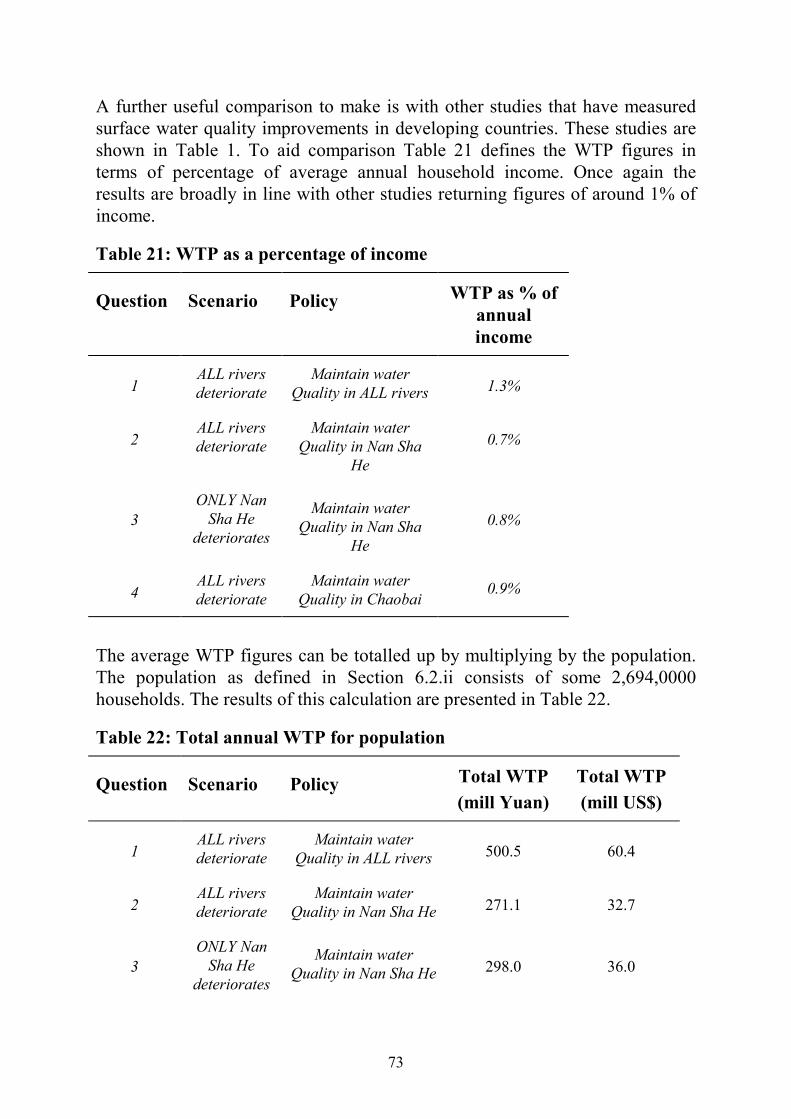
73

A further useful comparison to make is with other studies that have measured surface water quality improvements in developing countries. These studies are shown in Table 1. To aid comparison Table 21 defines the WTP figures in terms of percentage of average annual household income. Once again the results are broadly in line with other studies returning figures of around 1% of income.

Table 21: WTP as a percentage of income

Question Scenario Policy WTP as % of annual income


Maintain water Quality in ALL rivers 1.3%


Maintain water Quality in Nan Sha

He 0.7%

3 ONLY Nan

Sha He deteriorates

Maintain water Quality in Nan Sha

He 0.8%



0.9%

The average WTP figures can be totalled up by multiplying by the population. The population as defined in Section 6.2.ii consists of some 2,694,0000 households. The results of this calculation are presented in Table 22.

Table 22: Total annual WTP for population

Question Scenario Policy Total WTP (mill Yuan)

Total WTP (mill US$)


Maintain water Quality in ALL rivers 500.5 60.4


Maintain water Quality in Nan Sha He 271.1 32.7

3 ONLY Nan

Sha He deteriorates

Maintain water Quality in Nan Sha He 298.0 36.0

74


Maintain water Quality in Chaobai 330.8 40.0

The aggregated figures clearly display the considerable WTP of the population to maintain water quality standards in the rivers of the Beijing Metropolitan Region.

75

7. Implications and Conclusions

This paper reports on the results of a large-scale economic valuation study of river water quality improvements in the Beijing Metropolitan Region. A carefully designed contingent valuation questionnaire was administered to a random sample of 999 people in the Beijing area. The interviews were conducted both off-site and on-site at river locations. Several scenarios were proposed whereby river water quality would deteriorate; respondents were then asked for their willingness to pay to prevent deterioration of specific rivers (the Chaobai or the Nan Sha He) and of all the rivers in the area. The main conclusions that can be drawn from the study are the following:

• Contingent valuation, an economic valuation technique based on constructing hypothetical markets, was successfully administered in China. This result adds to the growing evidence that non-market valuation techniques developed in industrialised countries can translate successfully into the particular context of developing countries, where the population of interest may not know how to read or write, where ability to pay may be low and where markets may not be well developed.

• Beijing residents rank environmental problems as one of their top priorities; however, when asked about specific environmental problems, surface water quality comes only 4th, after air pollution, waste management and drinking water quality. This indicates that WTP for river water quality changes may not be very high.

• Non-use motivations appear to be the most important determinants of river preservation for the Chinese: the desire to preserve rivers for future generations or for third parties, for the sake of the animals and plants that find their habitat in river environments and to keep the option of having clean rivers in the future. This suggests that a very important part of the value of a particular river may be transferable to another rivers.

• Off-stream activities dominate recreational uses of Beijing rivers. ‘Walking’ and ‘relaxing and enjoying the scenery’ are the most popular activities, practised by 54% and 45% of the surveyed population, respectively. Only 20% of the people swim. This is consistent with the fact that rivers are generally considered to be polluted.

• There is a great disparity between perceived water quality at the Chaobai and the Nan Sha He rivers, the latter being considered to be much more polluted.

76

This corresponds to the scientific information available showing that residents of the Beijing Metropolitan Region have good knowledge about the state of local rivers.

• The pilot stages of the survey revealed an insensitivity to the scope of the injury, that is, to the specified changes in the level of pollution. This finding is common to other studies. Hence, the different perceived levels of pollution between rivers should not translate into different WTP amounts.

• Around 20% of the sample expressed a zero WTP for preservation of river water quality, which is consistent with the fact that surface water quality is not one of the top three major environmental concerns.

• Average WTP per household per year for the prevention of water quality deterioration was found to be 123 Yuan (US$15) for the Chaobai and 101 Yuan (US$12) for the Nan Sha He. As expected, these two values are not statistically different from one another although the two rivers are perceived to be very different. The implication is that transferability of values between rivers may be possible even though the rivers may be different.

• The WTP for preserving water quality at a particular river was also found to be independent of what happened to other rivers in the area. This results seems to support the thesis of low substitutability between rivers, i.e. low mobility amongst river users. It is also consistent with a strong non-use value component in the estimated values.

• Average WTP per household per year to maintain the quality of all Beijing rivers was estimated to be 186 Yuan (US$22). This value is significantly higher than the value of individual rivers like the Chaobai or the Nan Sha He. This means that the proposed scenario passed the scale test, i.e. the preservation of a small subset of rivers has a significantly lower value than that attributed to preserving a larger set of rivers. Aggregating over the target population yields an estimate of 500 million Yuan (US$60 million) for the preservation of all rivers in the area.

• As a proportion of income, the estimated values amount to 1.3% for all rivers and 0.8% for specific rivers. These results are reasonable and consistent to previous findings for both developed and developing countries.

• The estimated values also performed well in terms of standard tests of coherence and validity. Main determinants of the requested compensation amounts were the level of income and the frequency of use of the river.

77

• Methodologically, the study suggests that dichotomous choice elicitation procedures may not be the easiest way of eliciting respondents WTP values due to a tendency for ‘yes-saying’. Other elicitation techniques, such as payment card approaches, could arguably be more suited to the particular characteristics encountered in China. Further research is necessary to establish the validity of this assertion.

By and large, these results strike an optimistic note on the possibility of measuring the economic value of surface water quality improvements in China, even when non-use values predominate. On average, WTP for preventing river water quality from deteriorating is positive and amounts to around 1% of household income. These findings provide an important input into policy decisions in the sector.

78

References Box, G.E. and Cox, D.R. (1964) ‘An Analysis of Transformations’, Journal of Royal

Statistical Society, B(2), 211-252

Carson, R.T. and Mitchell, R.C. (1995) ‘Sequencing and Nesting in Contingent Valuation Surveys’, Journal of Environmental Economics and Management, 28, 155-173

Choe, K., Whittington, D. and Lauria, D. (1994) ‘The Economic Benefits of Surface water Quality Improvements in Developing Countries: A Case Study of Davao, Philippines’, Land Economics 72 (4), 519-537.

Halvorsen, B. (1996) ‘Ordering Effects in Contingent Valuation Surveys. Willingness to Pay for Reduce Health Damage from Air Pollution’, Environmental and Resource Economics, 8, 485-499.

Hanemann, W.M. (1984) ‘Welfare Evaluations in Contingent Valuation Experiments with Discrete Responses’, American Journal of Agricultural Economics, 66, 332-341

Hanemann, W.M. (1995) ‘Preference Uncertainty, Optimal Designs and Spikes’, in P. Johansson, B. Kristöm and K. Mäler (eds.) Current Issues in Environmental Economics, Manchester University Press, Manchester.

Hanemann, W.M., Loomis, J. and Kanninen, B. (1991) ‘Statistical Efficiency of Double-Bounded Dichotomous Choice Contingent Valuation’, American Journal of Agricultural Economics, 73, 1255-1263

Institute of Rural Economy and Yunnan Academy of Sciences (1995) ‘Kunming Ability and Willingness to Pay Survey’, Report to the Yunnan Environment Project, Yunnan.

Krinsky, I. and Robb, A.L. (1986) ‘On Approximating the Statistical Properties of Elasticities’ The Review of Economics and Statistics, 68, 715-719

Manski, C., and Lerman, S. (1977) ‘The Estimation of Choice Probabilities from Choice-Based Samples’, Econometrica, 45, 1977-1988.

McConnell, K. and Ducci, J. (1989) Valuing Environmental Quality in Developing Countries: Two Case Studies, Paper presented to Applied Social Science Association, Atlanta, Georgia.

Mitchell, R. and Carson, R. (1989) Using Surveys to Value Public Goods: The Contingent Valuation Method, John Hopkins Press, Baltimore.

Mourato, S. (1998) ‘Economic Valuation in Transition Economies: An Application of Contingent Valuation to Lake Balaton in Hungary’, in M. Acutt and P. Mason (eds.) Recent Advances in Environmental Economics, Edward Elgar, London, forthcoming.

National Oceanic and Atmospheric Administration (1993) ‘Report of the NOAA Panel on Contingent Valuation’, Federal Register, v.S8, No. 10, 4602-4614.

Zylicz, T., Bateman, I., Geourgiou, S., Markowska, A., Dziegielewska, D., Turner, R.K., Graham, A., Langford, I. (1995) ‘Contingent Valuation of Eutrophication Damage in the Baltic Sea Region’, CSERGE Working Paper GEC 95-03, Centre for Social and Economic Research on the Global Environment, University College London and University of East Anglia.

Date post:	24-Aug-2018
Category:	Documents
Upload:	votuyen
View:	215 times
Download:	0 times

WTP for Water Quality Improvements - UCL - London's … · The field work underlying this paper was...

Documents