44
www.sti-innsbruck.at © Copyright 2008 STI INNSBRUCK www.sti- innsbruck.at Neural Networks Intelligent Systems – Lecture 13 Prof. D. Fensel & R. Krummenacher
| Date post: | 22-Dec-2015 |
| Category: |
Documents |
| View: | 214 times |
| Download: | 1 times |

www.sti-innsbruck.at © Copyright 2008 STI INNSBRUCK www.sti-innsbruck.at
Neural Networks
Intelligent Systems – Lecture 13Prof. D. Fensel & R. Krummenacher
www.sti-innsbruck.at
Agenda
• Motivation
• (Artificial) Neural Networks
– Perceptrons and Activation Functions
• Neural Network Structures
– Single-Layer Feed-Forward
– Multi-Layer Feed-Forward
– Recurrent Networks
• Learning and Generalization
• Expressiveness of Multi-Layer Perceptrons
• Applications and Examples
• Summary and Conclusions

www.sti-innsbruck.at
Motivation
• A main motivation behind neural networks is the fact that symbolic rules do not reflect reasoning processes performed by humans.
• Biological neural systems can capture highly parallel computations based on representations that are distributed over many neurons.
• They learn and generalize from training data; no need for programming it all...
• They are very noise tolerant – better resistance than symbolic systems.
• In summary: neural networks can do whatever symbolic or logic systems can do, and more. In practice it is not that obvious however.

www.sti-innsbruck.at
Motivation
• Neural networks are stong in:
– Learning from a set of examples
– Optimizing solutions via constraints and cost functions
– Classification: grouping elements in classes
– Speech recognition, pattern matching
– Non-parametric statistical analysis and regressions

www.sti-innsbruck.at
Introduction: What are Neural Networks?
• Neural networks are networks of neurons as in the real biological brain.
• Neurons are highly specialized cells that transmit impulses within animals to cause a change in a target cell such as a muscle effector cell or glandular cell.
• The axon, is the primary conduit through which the neuron transmits impulses to neurons downstream in the signal chain
• Humans: 1011 neurons of > 20 types, 1014 synapses, 1ms-10ms cycle time
• Signals are noisy “spike trains” of electrical potential

www.sti-innsbruck.at
Introduction: What are Neural Networks?
• What we refer to as Neural Networks in the course are mostly Artificial Neural Networks (ANN).
• ANN are approximation of biological neural networks and are built of physical devices, or simulated on computers.
• ANN are parallel computational entities that consist of multiple simple processing units that are connected in specific ways in order to perform the desired tasks.
• Remember: ANN are computationally primitive approximations of the real biological brains.

www.sti-innsbruck.at
Comparison & Contrast
• Neural networks vs. classical symbolic computing1. Sub-symbolic vs. Symbolic2. Non-modular vs. Modular3. Distributed representation vs. Localist representation4. Bottom-up vs. Top-down5. Parallel processing vs. Sequential processing
• In reality however, it can be observed that the distinctions become increasingly less obvious!

www.sti-innsbruck.at
McCulloch-Pitts „Unit“ – Artificial Neurons
• Output is a „squashed“ linear function of the inputs:
• A clear oversimplification of real neurons, but its purpose is to develop understanding of what networks of simple units can do.

www.sti-innsbruck.at
Activation Functions
(a) is a step function or threshold function(b) is a sigmoid function 1/(1+e-x)
• Changing the bias weight w0,i moves the threshold location

www.sti-innsbruck.at
Perceptron
• McCulloch-Pitts neurons can be connected together in any desired way to build an artificial neural network.
• A construct of one input layer of neurons that feed forward to one output layer of neurons is called Perceptron.
www.sti-innsbruck.at
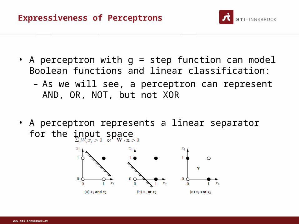
Expressiveness of Perceptrons
• A perceptron with g = step function can model Boolean functions and linear classification:
– As we will see, a perceptron can represent AND, OR, NOT, but not XOR
• A perceptron represents a linear separator for the input space

www.sti-innsbruck.at
Expressiveness of Perceptrons (2)
x2
x1
00
• Threshold perceptrons can represent only linearly separable functions (i.e. functions for which such a separation hyperplane exists)
• Such perceptrons have limited expressivity, but there exists an algorithm that can fit a threshold perceptron to any linearly separable training set.

www.sti-innsbruck.at
Example: Logical Functions
• McCulloch and Pitts: Boolean function can be implemented with a artificial neuron (not XOR).

www.sti-innsbruck.at
Example: Finding Weights for AND Operation
• There are two input weights W1 and W2 and a treshold W0. For each training pattern the perceptron needs to satisfay the following equation:
out = sgn(W1*in1 + W2*in2 – W0)
• For a binary AND there are four training data items available that lead to four inequalities:– W1*0 + W2*0 – W0 < 0 ⇒ W0 > 0– W1*0 + W2*1 – W0 < 0 ⇒ W2 < 0– W1*1 + W2*0 – W0 < 0 ⇒ W1 < 0– W1*1 + W2*1 – W0 ≥ 0 ⇒ W1 + W2 ≥ W0
• There is an obvious infinite number of solutions that realize a logical AND; e.g. W1 = 1, W2 = 1 and W0 = 1.5.

www.sti-innsbruck.at
Limitations of Simple Perceptrons
• XOR:– W1*0 + W2*0 – W0 < 0 ⇒ W0 > 0– W1*0 + W2*1 – W0 ≥ 0 ⇒ W2 ≥ 0– W1*1 + W2*0 – W0 ≥ 0 ⇒ W1 ≥ 0– W1*1 + W2*1 – W0 < 0 ⇒ W1 + W2 < W0
• The 2nd and 3rd inequalities are not compatible with inequality 4, and there is no solution to the XOR problem.
• XOR requires two separation hyperplanes!
• There is thus a need for more complex networks that combine simple perceptrons to address more sophisticated classification tasks.

www.sti-innsbruck.at
Neural Network Structures
• Mathematically artificial neural networks are represented by weighted directed graphs.
• In more practical terms, a neural network has activations flowing between processing units via one-way connections.
• There are three common artificial neural network architectures known:
– Single-Layer Feed-Forward (Perceptron)
– Multi-Layer Feed-Forward
– Recurrent Neural Network

www.sti-innsbruck.at
Single-Layer Feed-Forward
• A Single-Layer Feed-Forward Structure is a simple perceptron, and has thus
– one input layer
– one output layer
– NO feed-back connections
• Feed-forward networks implement functions, have no internal state (of course also valid for multi-layer perceptrons).

www.sti-innsbruck.at
Single-Layer Feed-Forward: Example
• Output units all operate separately – no shared weights (the study can be limited to single output perceptrons!)
• Adjusting weights moves the location, orientation, and steepness of cliff.

www.sti-innsbruck.at
Multi-Layer Feed-Forward
• Multi-Layer Feed-Forward Structures have:
– one input layer
– one output layer
– one or MORE hidden layers of processing units
• The hidden layers are between the input and the output layer, and thus hidden from the outside world: no input from the world, not output to the world.

www.sti-innsbruck.at
Recurrent Network
• Recurrent networks have at least one feedback connection:
– They have thus directed cycles with delays: they have internal state (like flip flops), can oscillate, etc.
– The response to an input depends on the initial state which may depend on previous inputs – can model short-time memory
– Hopfield networks have symmetric weights (Wij = Wji)
– Boltzmann machines use stochastic activation functions,
≈ MCMC in Bayes nets

www.sti-innsbruck.at
Building Neural Networks
• Building a neural network for particular problems requires multiple steps:1. Determine the input and outputs of the problem;2. Start from the simplest imaginable network, e.g. a single
feed-forward perceptron;3. Find the connection weights to produce the required
output from the given training data input;4. Ensure that the training data passes successfully, and
test the network with other training/testing data;5. Go back to Step 3 if performance is not good enough;6. Repeat from Step 2 if Step 5 still lacks performance; or7. Repeat from Step 1 if the network does still not perform
well enough.

www.sti-innsbruck.at
Learning and Generalization
• Neural networks have two important aspects to fulfill:
– They must learn decision surfaces from training data, so that training data (and test data) are classified correctly;
– They must be able to generalize based on the learning process, in order to classify data sets it has never seen before.
• Note that there is an important trade-off between the learning behavior and the generalization of a neural network: The better a network learns to successfully classify a training sequence (that might contain errors) the less flexible it is with respect to arbitrary data.

www.sti-innsbruck.at
Learning vs. Generalization
• Noise in the actual data is never a good thing, since it limits the accuracy of generalization that can be achieved no matter how extensive the training set is.
• Non-perfect learning is better in this case!
• However, injecting artificial noise (so-called jitter) into the inputs during training is one of several ways to improve generalization
„Perfect“ learning achieves the dotted separation, while the desired one is in fact given by the solid line.
Regression Classification

www.sti-innsbruck.at
Estimation of Generalization Error
• There are many methods for estimating generalization error. • Single-sample statistics
– In linear models, statistical theory provides estimators that can be used as crude estimates of the generalization error in nonlinear models with a "large" training set.
• Split-sample or hold-out validation. – The most commonly used method for estimating the
generalization error in ANN is to reserve some data as a "test set”, which must not be used during training.
– The test set must represent the cases that the ANN should generalize to. A re-run with the test set provides an unbiased estimate of the generalization error, provided that the test set was chosen randomly.
– The disadvantage of split-sample validation is that it reduces the amount of data available for both training and validation.

www.sti-innsbruck.at
Estimation of Generalization Error
• Cross-validation (e.g., leave one out). – Cross-validation is an improvement on split-sample validation
that allows the use of all of the data for training. – The disadvantage of cross-validation is that the net must be
retrained many times. • Bootstrapping.
– Bootstrapping is an improvement on cross-validation that often provides better estimates of generalization error at the cost of even more computing time.
• No matter which method is applied, the estimate of the generalization error of the best network will be optimistic.
• If several networks are trained using one data set, and a second (validation set) is used to decide which network is best, a third test set is required to obtain an unbiased estimate of the generalization error of the chosen network.

www.sti-innsbruck.at
Learning Neural Networks
• Learning is based on training data, and aims at appropriate weights for the perceptrons in a network.
• Direct computation is in the general case not feasible.
• An initial random assignment of weights simplifies the learning process that becomes an iterative adjustment process.
• In the case of single perceptrons, learning becomes the process of moving hyperplanes around; parametrized over time t: Wi(t+1) = Wi(t) + ΔWi(t)

www.sti-innsbruck.at
Perceptron Learning
• The squared error for an example with input x and true output y is
• Perform optimization search by gradient descent
• Simple weight update rule
– positive error ⇒ increase network output: • increase weights on positive inputs, • decrease on negative inputs

www.sti-innsbruck.at
Perceptron Learning (2)
• The weight updates need to be applied repeatedly for each weight Wi in the network, and for each training suite in the training set.
• One such cycle through all weighty is called an epoch of training.
• Eventually, mostly after many epochs, the weight changes converge towards zero and the training process terminates.
• The perceptron learning process always finds a set of weights for a perceptron that solves a problem correctly with a finite number of epochs, if such a set of weights exists.
• If a problem can be solved with a separation hyperplane, then the set of weights is found in finite iterations and solves the problem correctly.

www.sti-innsbruck.at
Perceptron Learning (3)
• Perceptron learning rule converges to a consistent function for any linearly separable data set
• Perceptron learns majority function easily, Decision-Tree is hopeless
• Decision-Tree learns restaurant function easily, perceptron cannot represent it.

www.sti-innsbruck.at
Multi-Layer Perceptrons
• Multi-Layer Perceptrons (MLP) have fully connected layers.
• The numbers of hidden units is typically chosen by hand; the more layers, the more complex the network (Step 2 of Building a Neural Network)
• Hidden layers enlarge the space of hypotheses that the network can represent.
• Learning done by back-propagation algorithm → errors are back-propagated from the output layer to the hidden layers.

www.sti-innsbruck.at
Back-Propagation Learning
• Output layer: same as for single-layer perceptron,
where
• Hidden layer: back-propagate the error from the output layer:
• Update rule for weights in hidden layer:
• Most neuroscientists deny that back-propagation occurs in the brain.

www.sti-innsbruck.at
Back-Propagation Learning (2)
• At each epoch, sum gradient updated for all examples
• Training curve for 100 restaurant examples converges to a perfect fit to the training data
• Typical problems: slow convergence, local minima

www.sti-innsbruck.at
Back-Propagation Learning (3)
• Learning curve for MLP with 4 hidden units (as in our restaurant example):
• MLPs are quite good for complex pattern recognition tasks, but resulting hypotheses cannot be understood easily

www.sti-innsbruck.at
Expressiveness of MLPs
• 2 layers can represent all continuous functions• 3 layers can represent all functions
• Combine two opposite-facing threshold functions to make a ridge.
• Combine two perpendicular ridges to make a bump.• Add bumps of various sizes and locations to fit any surface• The required number of hidden units grows exponentially with
the number of inputs (2n/n for all boolean functions)

www.sti-innsbruck.at
Expressiveness of MLPs (2)
• The more hidden units, the more bumps• Single, sufficiently large hidden layer can represent any
continuous function of the inputs with arbitrary accuracy• Two layers are necessary for discontinuous functions• For any particular network structure, it becomes harder to
characterize exactly which functions can be represented and which ones cannot.

www.sti-innsbruck.at
Simple MLP Example
• XOR Problem: Recall that XOR cannot be modeled with a Single-Layer Feed-Forward perceptron.
1
2
3

www.sti-innsbruck.at
Number of Hidden Layers
• Rule of Thumb 1: even if the function to learn is slightly non-linear, the generalization may be better with a simple linear model than with a complicated non-linear model; if there is too little data or too much noise to estimate the non-linearities accurately.
• In MLPs with threshold activation functions, two hidden layers are needed for full generality.
• In MLPs with any continuous non-linear hidden-layer activation functions, one hidden layer with an arbitrarily large number of units suffices for the "universal approximation" property. However, there is no theory yet that tells how many hidden units are needed to approximate any given function.
www.sti-innsbruck.at
Number of Hidden Layers (2)
• Rule of Thumb 2: If there is only one input, there seems to be no advantage to using more than one hidden layer; things get much more complicated when there are two or more inputs.
• Using two hidden layers complicates the problem of local minima, and it is important to use lots of random initializations or other methods for global optimization. Local minima with two hidden layers can have extreme spikes or blades even when the number of weights is much smaller than the number of training cases.
• More than two hidden layers can be useful in certain architectures such as cascade correlation, and in special applications, such as the two-spirals problem and ZIP code recognition.

www.sti-innsbruck.at
Hidden Layers in Example
1st layer draws linear boundaries
2nd layer combines the boundaries.
3rd layer can generate arbitrarily boundaries.

www.sti-innsbruck.at
Application Examples
• To conclude this lecture we take a look at some real world example:– Handwriting Recognition– Time Series Prediction– Bioinformatics– Kernel Machines (Support Vectore Machines)
• Endless further examples:– Data Compression– Financial Predication– Speech Recognition– Computer Vision– Protein Structures– ...

www.sti-innsbruck.at
Application Example: Handwriting
• Many applications of MLPs: speech, driving, handwriting, fraud detection, etc.
• Example: handwritten digit recognition
– automated sorting of mail by postal code
– automated reading of checks
– data entry for hand-held computers

www.sti-innsbruck.at
Application Example: Time Series Prediction
• Neural networks can help to transform temporal problems into simple input-output mappings by taking m time series data samples from the past as input in order to compute a prediction for the next instance of the future as output: s(t+1) = ANN(s(t), s(t-1), ..., s(t-m)).
• By using predicted values as input (simulating a past in the future), time series predication allows estimates for points in time further in the future.
• Examples of time series prediction problems are found in the financial world (stock predictions), climate research (also weather prediction), or customer/passenger estimates.

www.sti-innsbruck.at
Application Example: Kernel Machines
• New family of learning methods: support vector machines (SVMs) or, more generally, kernel machines
• Combine the best of single-layer networks and multi-layer networks– use an efficient training algorithm– represent complex, nonlinear functions
• Techniques– kernel machines find the optimal linear separator; i.e. the one
that has the largest margin between it and the positive examples on one side and the negative examples on the other
– quadratic programming optimization problem

www.sti-innsbruck.at
Summary and Conclusions
• Most brains have lots of neurons, each neuron approximates a linear-threshold unit.
• Perceptrons (one-layer networks) approximate neurons, but are as such insufficiently expressive.
• Multi-layer networks are sufficiently expressive; can be trained to deal with generalized data sets, i.e. via error back-propagation.
• Multi-layer networks allow for the modeling of arbitrary separation boundaries, while single-layer perceptrons only provide linear boundaries.
• Endless number of applications: Handwriting Recognition, Time Series Prediction, Bioinformatics, Kernel Machines (Support Vectore Machines), Data Compression, Financial Predication, Speech Recognition, Computer Vision, Protein Structures...


