Hodrick-Prescott filter • Assume that the series y t is the sum of the growt component g t and a cyclical component c t y t = c t + g t for t =1,...,T • The growth component g t varies smoothly over time • The cyclical component c t is in average equal to zero • Assume taht measure of smoothness of {g t } path is the sum of squares of its second differances Macroeconometrics, WNE UW, Copyright c 2007 by Jerzy Mycielski 1
Transcript
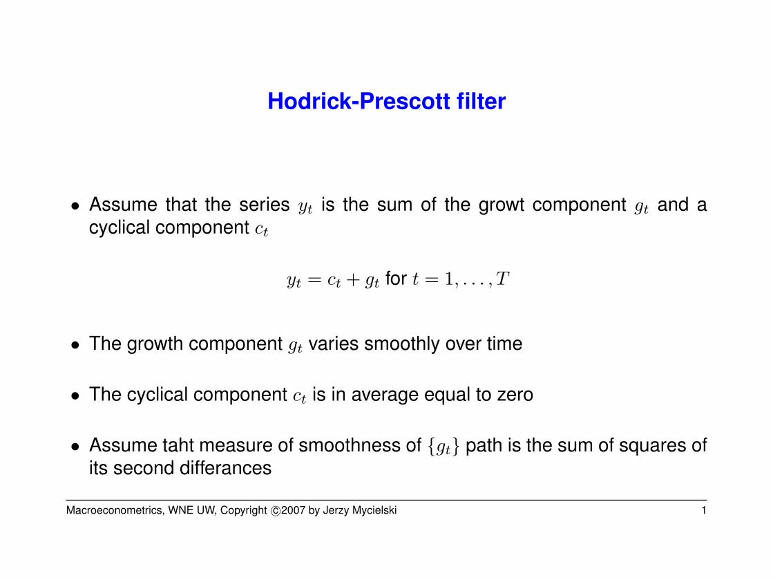
Hodrick-Prescott filter
• Assume that the series yt is the sum of the growt component gt and acyclical component ct
yt = ct + gt for t = 1, . . . , T
• The growth component gt varies smoothly over time
• The cyclical component ct is in average equal to zero
• Assume taht measure of smoothness of {gt} path is the sum of squares ofits second differances
• The to filter ct and gt we have to solve following maximization problem
min{gt}T
t=−1
{T∑
t=1
c2t + λ
T∑t=1
∆2gt
}
where ct = yt − gt
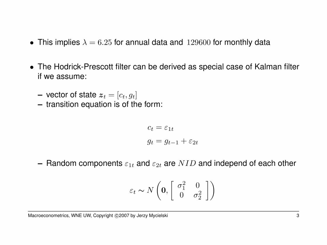
• λ is a positive number which panelizes the variability in growth componentseries
• The larger is λ the smoother is the solution, for λ → ∞ the solution of theproblem is the OLS fit of linear trend
• Hodrick and Prescott suggested to use λ = 1600 for quarterly data.Rawn and Uhlig (2002) shown that λ should be proprtional to 4 powerof frequency observation rations.
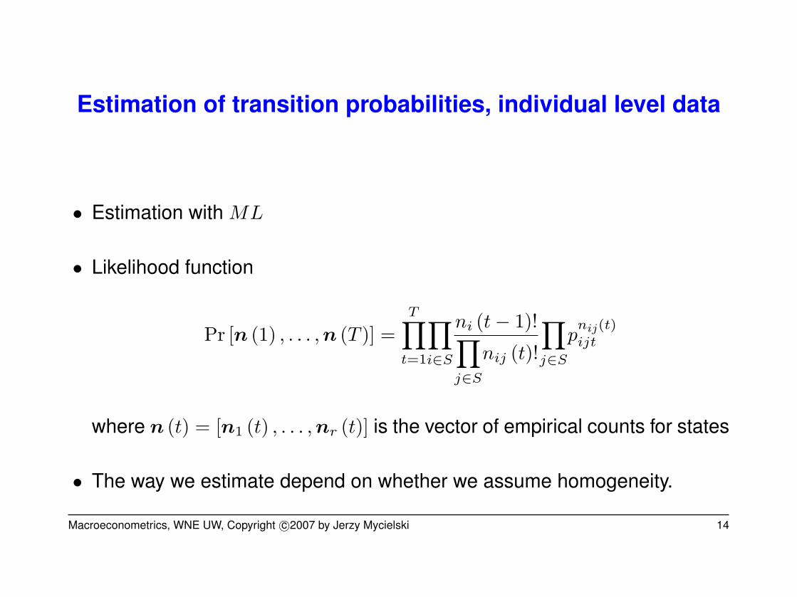
• Under homogeneity the ML estimator of transition probabilities hasfollowing intuitive form:
p̂ij =nij
ni
where
nij =T−1∑t=1
nijt
ni =T−1∑t=1
∑
j∈S
nijt
• So the ML estimator for pij is the proportion of transition between state ito j for all times 1, . . . , T , in total number os observations observed in statei for times 1, . . . , T − 1
• ML estimator of transiotion probabilities for nonhomogenous Markow
Estimation of transition probabilities, aggregated data
• For aggregated data we only observe the numbers of units (or fractions)observed in given states in time t
• Conditional expected value of the number of observations in state j in timet from ni observation, which were obseved to be in state i in time t − 1 isequal to:
where pj is j-th column of the matrix of transition probabilities and rowvector N (t− 1) = [n1 (t) , . . . , nr (t)] is a vector of numbers of units beingin each state


![b arXiv:1408.5332v1 [math.OC] 22 Aug 2014 › pdf › 1408.5332.pdf · xt+1 i = x t+ L( )(g xt); (1) where xt i is the pollen ior solution vector x iat iteration t, and g is the current](https://static.documents.pub/doc/80x56/5f0440547e708231d40d0e0d/b-arxiv14085332v1-mathoc-22-aug-2014-a-pdf-a-14085332pdf-xt1-i-x.jpg)


