XCP MEAlSUREMENTS OFF CALIFORNIA IN CRUISE · dred CTD and AMP 1 profiles of temperature and...

>fiD-8i3-3 051 XCP MEAlSUREMENTS OFF CALIFORNIA IN OCTOBER 1982: CRUISE 1/1REPORT AiND PRELIM (U) WASHINGTON UNIV' SEATTLE APPLIEDPHYSICS LABE EA DAAROHO AU8- PL-W-8310

UNCLASSIFIED N000I4-8--03 / /1 N

W.2.11111 1.0 ~~&66wFA

MICROCOPY RESOLUTION TEST CHARTNATIONAL BUREAU OF STANOARDS-1963-A

Applied ~ ~ Phsc aoatr nvriy0fWsigo

I.

p XCP Measurements Off California in October 1982:N Cruise Report and Preliminary Results

Eric A. D'Asaro

APL-UW 831012 August 1983

DTICEL CTE,

'~\SEP 2 8 1g

I s tor For--/

a; 0A'iati Applied Physics Laboratory

University of Washingtonon/~ Contract NOOO 14-82-C- 0038

SAveltubil.11Y (lodes

:Avai. zind/Or

This document hasn been approved____________________for Public release and sale; its V

d;,rihution is unlimted.

-7 .7

Acknowledgments

% This work was done under the sponsorship of the Naval Ocean Research and Develop-mernt Activity, Code 500. Contract N00014-B2-C-0038. Satellite images from the ScrippsRemote Sensing Facility were supported by Office of Naval Research Contract N00014-B1-K0095. Additional satellite images were supplied free of charge by the National Oceanicand Atmospheric Administration. National Environmental Satellite Service. Redwood City.CA. offlice.

Ze..

UNIVERSITY OF WASHINGTON APPLIED PHYSICS LABORATORY

* AB9MCT

Sixty-nine profiles of horizontal velocity and temperature from the surface to about800 m were made using the Expendable Current Profiler (XCP) during De Steiguer cruise1212. 7-18 October 1982. The XCP's were deployed in a 6 day time series behind a dro-gued buoy and in a 275 n.mi. zigzag spatial survey. Satellite infrared images were used to

, locate a cruise area away from strong mesoscale features. The measurements weredesigned to estimate the horizontal coherence function of the near-inertial frequencyinternal wave field for comparison with similar measurements made in the Sargasso Sea.It was found that the near-inertial waves are a dominant feature of the velocity field.Significant coherence exists between nearby profiles. It will, therefore, be possible tocompute a correlation function for these data as planned. A near-surface feature withpeak-to-peak velocities of 70 cm/s was observed and partially surveyed.

APL-UW 8310 iii

* .- c ... ~. . . . . . *. - .|

.7.7---. :77.1 -.

IEW]I


TABLE OF CONTENTS

INTRODTE TY.....................................................................................

INTRODEGY.ION.................................................................................. 1

Location .....................................................................................

Time Series Measurements..................................................................... 1

*Hydrographic Data ............................................................................ 2

Spatial Survey.................................................................................... 2

NCRUISE AND DATA DESCRIPTION ............................................................... 4

Discussion of Data ............................................................................... 1?7

- ~ RECOMMENDATIONS ............................................................................ 23

Routine Oceanographic Measurements....................................................... 23

Specialized Scientific Measurements ......................................................... 25

REFERENCES..................................................................................... 26

'-47

iv APLUW 831


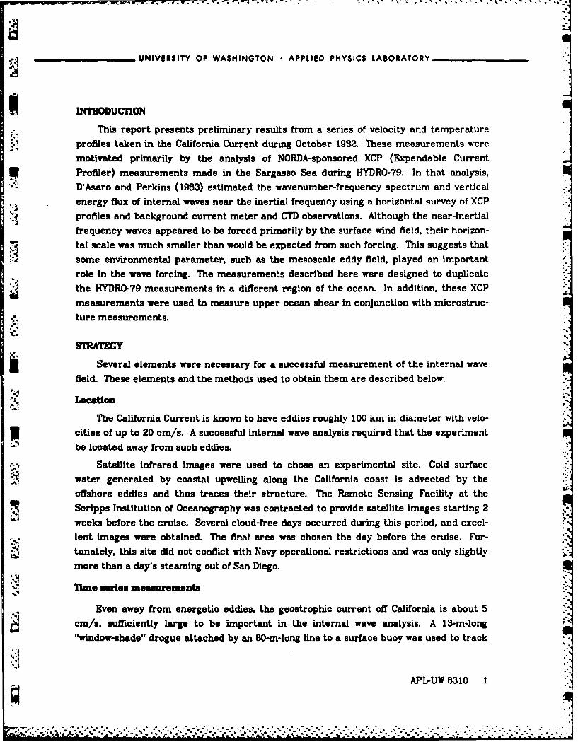
IRODUCON

This report presents preliminary results from a series of velocity and temperature

profiles taken in the California Current during October 1982. These measurements were

motivated primarily by the analysis of NORDA-sponsored XCP (Expendable Current

Profiler) measurements made in the Sargasso Sea during HYDRO-79. In that analysis,

D'Asaro and Perkins (1963) estimated the wavenumber-frequency spectrum and vertical

energy flux of internal waves near the inertial frequency using a horizontal survey of XCP

profiles and background current meter and CTD observations. Although the near-inertial

frequency waves appeared to be forced primarily by the surface wind field, their horizon-

tal scale was much smaller than would be expected from such forcing. This suggests that

some environmental parameter, such as the mesoscale eddy field, played an important

role in the wave forcing. The measurement described here were designed to duplicate

the HYDRO-79 measurements in a different region of the ocean. In addition, these XCP

measurements were used to measure upper ocean shear in conjunction with microstruc-

ture measurements.

STRATGY

Several elements were necessary for a successful measurement of the internal wave

field. These elements and the methods used to obtain them are described below..%

Location

The California Current is known to have eddies roughly 100 km in diameter with velo-

cities of up to 20 cm/s. A successful internal wave analysis required that the experiment

be located away from such eddies.

Satellite infrared images were used to chose an experimental site. Cold surface

water generated by coastal upwelling along the California coast is advected by the

offshore eddies and thus traces their structure. The Remote Sensing Facility at the

Scripps Institution of Oceanography was contracted to provide satellite images starting 2

weeks before the cruise. Several cloud-free days occurred during this period, and excel-

lent images were obtained. The final area was chosen the day before the cruise. For-

tunately, this site did not conflict with Navy operational restrictions and was only slightly

more than a day's steaming out of San Diego.

Time series measurements

Even away from energetic eddies, the geostrophic current off California is about 5

cm/s, sufficiently large to be important in the internal wave analysis. A 13-m-long

"window-shade" drogue attached by an 80-m-long line to a surface buoy was used to track

APL-UM 0310 1

I -7'


the water below the mixed layer for 5 days and thus estimate the near-surface geos-

trophic velocity. A time series of XCP profiles was made at the drifting buoy to separate

the near-inertial, low frequency geostrophic, and high frequency internal wave com-

ponents of the velocity field. The sampling was one quarter of an inertial period. This

time series also provided shear information for use with the microstructure profiles taken

during this time. Because internal waves are advected by the geostrophic flow, a time

series following a drifting buoy is much less affected by advection than is a moored time

series. Thus, no correction for adveetion is necessary here, unlike the HYDRO-79 analysis.

Hydrographic data

The internal wave field depends critically on the oceanic density profile. Several hun-

dred CTD and AMP 1 profiles of temperature and salinity were taken in the upper 200 m

near the drifting buoy. Three CTD profiles were made to 600 m. These profiles will allow

the mean density profile, the mean T/S relation, and the T/S variability to be computed. -

In addition, 37 XBT's were launched during the spatial survey to help determine the geos-

trophic shear in the upper ocean.

Spatial survey

The major goal of these measurements was to determine the spatial correlation func- Wtion of the internal wave field near the inertial frequency, using the methods of D'Asaro

and Perkins (1983) and D'Asaro (1983). This required a spatial survey of XCP profiles sub-

ject to several constraints:

(1) The survey must cover an area, rather than extend along a line, so that the

isotropy of the internal wave field can be observed.

(2) If the correlation length of the internal wave field is roughly A, the survey must

sample an area much larger than X2 so that many independent realizations of

the internal wave field are sampled.

(3) The survey must contain probe separations both much smaller and much

larger than A so that the correlation function can be determined for a variety

of spatial lags. The small spatial lags and large spatial lags must be about

equally distributed throughout the survey.

(4) Probe pairs separated by short spatial distances, 5 km or less, must be taken

at short temporal separations, much less than an inertial period; pairs with

IAPI.UW's Advanced Moreruniture Profier

2 APL-UW 8310

2,

.= A-T - -.- -....- - -. . . . . ....-- "-- -..

UNIVERSITY OF WASHINGTON• APPLIED PHYSICS LABORATORY__

longer spatial separations can have longer temporal separations. This allows

"inertial rotation" to be used in the construction of the correlation function

(DAsaro and Perkins. 1963).

(5) The survey must use only 40 XCP's, assuming a 20% failure rate, and be exe-

cutable from a single ship within 2 days.

Considerable effort was spent designing sampling patterns. For a fixed number of

-.. probes, the primary trade-off is between condition 2. which requires a large pattern for

statistical reliability, and condition 3. which requires probes at small separations for an

accurate correlation function. An acceptable sampling pattern was required to have at

least 10 degrees of freedom at each separation. The degrees of freedom were computed

using the methods described by D'Asaro (1983) assuming a correlation scale of 50 km.

Originally, the sampling pattern was designed around the drifting buoy. Once at sea,

however, it was found that the radar transponder on the buoy was not properly tuned to

the ship's radar. The ship therefore had to stay within 5 km or so of the buoy, making it

impossible to execute the survey as planned. Instead, a modified survey was executed

after the buoy was recovered.

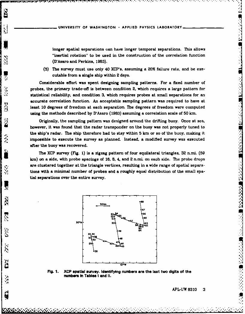
The XCP survey (Fig. 1) is a zigzag pattern of four equilateral triangles, 32 n.rni. (59

km) on a side, with probe spacings of 16, 8, 4. and 2 n.mL on each side. The probe drops

are clustered together at the triangle vertices, resulting in a wide range of spatial separa-

tions with a minimal number of probes and a roughly equal distribution of the small spa-

tial separations over the entire survey. r r67

53 66

5. 5665

30N50 636162

49 64

33,34 4 6

15

121W

Fig. 1. XCP spatial survey. Identifying numbers are the last two digits of thenumbers In Tables I and II.

APL-UW 0310 3

o',


CUISE AND DATA DESCRIPTION

All data reported here are associated with the USNS De Steiguer cruise 1212, 7-18

October 1982. Michael Gregg, chief scientist, directed the microstructure measurements,

CTD operations, and the drogued buoy deployment and recovery. XCP's manufactured by

the Sippican Corporation were deployed by Eric D'Asaro and Pat McKeown with the assis-

tance of other scientific personnel using standard APL-UW deck gear and procedures(Sanford et aL, 1982).

Of the 70 XCP probes taken on board, one was dead, and four were improperly

launched. Of the remaining 65 probes. 89% produced usable data and 62% functioned

nearly perfectly. This is a somewhat higher failure rate than has typically been found inAPL cruises and may partially be due to the use of less experienced personnel in the

launching procedure. In particular, data from several probes were lost when a minor vari-

ation in the launching procedure resulted in the XCP wire snagging on the launch tube.

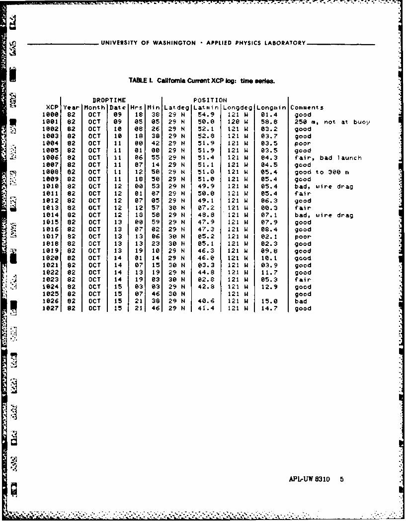
The location and times of all XCP deployments are shown in Tables I and II. The first

28 probes were launched within a few hundred meters of the drifting buoy. The

remainder of the probes were launched in the spatial pattern shown in Fig. 1.

The drift track of the buoy and the pattern of the spatial survey are shown super-posed on a satellite sea surface temperature image in Fig. 2. The experimental area isseen to be in a region of smooth sea surface temperature variation, well away from any

obvious eddies. A map of the 15*C isotherm constructed from the XCP and XBT tempera-ture data taken during the spatial survey (Fig. 3) similarly shows no evidence of an eddy.

The geostrophic shear between 400 m and the surface estimated from the mean isothermtilt in Fig. 3 is in rough agreement with the 6 cm/s mean southwesterly drift of the dro-

gued buoy over its 6 day deployment.

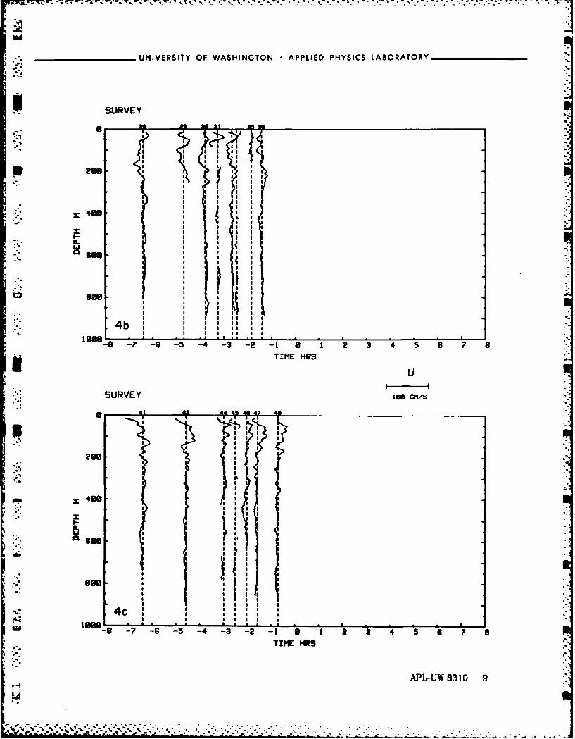
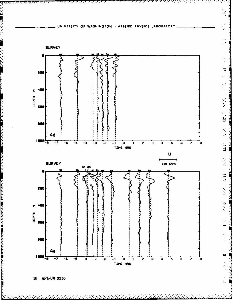
The east, north, and temperature data from all XCP profiles are shown in Figs. 4. 5,and 6 respectively. These profiles have been edited both by hand and using the normal

XCP noise criterion. A vertical mean was removed from each velocity component.

Profiles from the buoy time series are displayed in Figs. 4a, 5a, and 6a. Profiles from thespatial survey are shown in Figs. 4b-e, 5b-e, and 6b-e. In each of these figures the profiles

are displaced horizontally so that the origin of the plot corresponds to the time of launch

relative to an arbitrary origin, as displayed on the bottom axis. Each profile is identified

by the number on the upper axis, which corresponds to the number in Table I with thefirst two digits removed.

4 APL-UW 8310

• " :i' l'- o' 'l:-' ' I , - ' ' " " n ' ' ' ' ' ' ' ' " ' " " ;, "" :i " ':' i':': -" n " . ' . "

j% UNIVERSITY OF WASHINGTON APPLIED PHYSICS LABORATORY

STABLE 1. Callfonia Currnt XCP log: time seri.

DROPTIME POSITIONXCP Year Month Date Hrs Min Latdeg Latmin Longdeg Longmin Comments100 82 OCT 09 18 38 29 N 54.9 121 W 81.4 good

! 1001 82 OCT 09 05 05 29 N 50.0 120 W 58.8 250 m, not at buoV_ 1002 82 OCT 10 08 26 29 N 52.1 121 W 83.2 good

1003 82 OCT 18 18 38 29 N 52.8 121 W 03.7 good1004 82 OCT 11 00 42 29 N 51.9 121 W 03.5 poor1005 82 OCT 11 01 00 29 N 51.9 121 W 03.5 good1006 82 OCT 11 06 55 29 N 51.4 121 W 04.3 fair, bad launch1007 82 OCT 11 07 14 29 N 51.1 121 W 84.5 good1088 82 OCT 11 12 50 29 H 51.0 121W 05.4 good to 300 m

" 1009 82 OCT 11 18 50 29 N 51.0 121 W 85.4 good1010 82 OCT 12 00 53 29 N 49.9 121 W 05.4 bad, wire drag1011 82 OCT 12 01 07 29 N 50.0 121 W 05.4 fair1012 82 OCT 12 07 05 29 N 49.1 121 W 06.3 good1013 82 OCT 12 12 57 30 H 07.2 121W 00.3 fair1014 82 OCT 12 18 58 29 N 48.8 121 W 07.1 bad, wire drag1015 82 OCT 13 00 59 29 N 47.9 121 W 07.9 good1016 82 OCT 13 07 02 29 N 47.3 121 W 08.4 good

S 1017 82 OCT 13 13 06 30 N 05.2 121 W 02.1 poor

1618 82 OCT 13 13 23 30 N 05.1 121 W 02.3 good' 1019 82 OCT 13 19 10 29 N 46.3 121 W 09.8 good1020 82 OCT 14 81 14 29 N 46.0 121 W 10.1 good1021 82 OCT 14 07 15 30 N 03.3 121 W 03.9 good1022 82 OCT 14 13 19 29 N 44.8 121 W 11.7 good1023 82 OCT 14 19 03 30 N 02.8 121W 05.3 fair

.. 1824 82 OCT 15 03 03 29 N 42.8 121 W 12.9 good1025 82 OCT 15 07 46 30 N 121 W good1026 82 OCT 15 21 38 29 N 40.6 121 W 15.0 bad1027 82 OCT '5 21 46 29 N 41.4 121 W 14.7 good

A.8

APL.UW 8310 5

i '2,4 .. . * . "" ,". - .% ; ,. - . . L . .

-


TABLE I. California Current XCP log: survey.

DROPTIME POSITIONXCP Year Month Date Hrs Min Latdeg Latmin Longdeg Longrm in Comments1028 82 OCT 16 04 58 29 N 01.6 122 W 07.5 good1029 82 OCT 16 06 41 29 N 16.6 122 W 10.4 good1030 82 OCT 16 07 35 29 N 24.6 122 W 12.4 good1031 82 OCT 16 08 07 29 N 28.2 122 W 13.5 fair1032 82 OCT 16 08 14 29 H 28.5 122 W 13.6 no data1033 82 OCT 16 08 43 29 N 31.8 122 W 14.1 fair1034 82 OCT 16 08 55 29 N 32.4 122 W 14.2 poor1835 82 OCT 16 09 32 29 N 30.7 122 W 9.4 150 m only1036 82 OCT 16 09 41 29 N 30.5 122 W 9.0 poor1037 82 OCT 16 09 49 29 N 30.4 122 W 8.7 bad1038 82 OCT 16 09 58 29 N 30.2 122 W 8.3 good1039 82 OCT 16 10 59 29 H 26.9 121 W 58.2 bad, wire drag1040 82 OCT 16 11 51 29 N 24.3 121 W 49.6 bad, wire drag1041 82 OCT 16 12 49 29 N 21.5 121 W 39.9 good1042 82 OCT 16 14 39 29 N 16.3 121 W 22.5 good1043 82 OCT 16 15 41 29 N 15.0 121 W 16.7 bad, no data1044 82 OCT 16 16 14 29 N 12.4 121 W 8.9 fair1045 82 OCT 16 16 43 29 N 11.8 121 W 5.8 poor1046 82 OCT 16 17 12 29 N 16.0 121 W 7.1 good1047 82 OCT 16 17 39 29 N 19.2 121 W 8.3 good1048 82 OCT 16 16 31 29 N 26.8 121 W 10.7 good U1049 82 OCT 16 20 11 29 N 42.2 121 W 13.6 good1050 "2 OCT 16 21 54 29 N 57.8 121 W 17.6 good1851 82 OCT 16 22 53 30 N 6.5 121 W 19.4 poor1052 82 OCT 16 23 31 30 N 18.9 121 W 20.2 good to 200 m1053 82 OCT 17 00 01 30 N 14.7 121 W 20.3 good to 80 m1054 82 OCT 17 00 28 30 N 14.0 121 W 16.9 good1855 82 OCT 17 01 82 30 N 12.6 121 W 12.4 good1056 82 OCT 17 01 50 30 N 07.6 121 W 83.1 good, noisy1057 82 OCT 17 03 26 30 N 2.3 120 W 6.5 good1058 82 OCT 17 05 08 29 N 57.4 120 W 28.9 good1059 82 OCT 17 06 03 29 N 55.1 120 W 20.0 good to 120 m'1860 82 OCT 17 06 10 29 N 55.0 120 W 19.7 good1061 82 OCT 17 06 46 29 N 54.2 120 W 14.4 fair, noisy -1062 82 OCT 17 07 13 29 N 53.3 120 W 10.8 good to 200 m1063 82 OCT 17 07 47 29 N 57.4 120 W 11.6 good1064 82 OCT 17 08 42 29 N 55.5 120 W 20.1 good1065 82 OCT 17 18 31 30 N 8.3 120 W 14.5 good to 360 m1066 82 OCT 17 11 36 30 N 16.7 120 W 17.0 good1067 82 OCT 17 12 39 30 H 24.7 120 W 18.8 good1068 82 OCT 17 14 35 30 N 40.7 120 W 21.5 good

'of

'S.'.

6 APL-UW 8310

Ae. el1

7:1-K 47


1*

. Fig. 2. Buoy drift track and spatial survey pattern superposed on infraredsatellite picture of sea surface temperature taken at 2239 GMT, 16October 1982.

A H 1

L f-.c. . . ,. -... . . . . . . . . . . . . .

.41


, /I120 M

90m

90 V

Fig. 3. Depth of the 1 60 C isotherm from XCP and XBT data taken during thespatial survey. XCP depths were increased by 5 m to best matchXBT depths.

.4U

TIME SERIES e cM/s0607 1718

4eW

e-

I I MEH R

* II I|I II I I "-

Fig. 4. East velocity component for all XCP data. Vertical dashed linescorrespond to profile time relative to an arbitrary reference timedisplayed on the bottom axis. Profile Identification numbers on thetop axis correspond to the last two digits of the numbers in Tables Iand II.

8''8

8 PLU 81

;.' 84

" r ',¢ '.. . . . . . . . . . . . . . . . . ' ' / , I ( / ' t

_____ ____ UNIVERSITY OF WASHINGTON APPLIED PHYSICS LABORATORY

S eSURVEY

• see .

' 4bia- 7 -6 -a - -3 -2 '2 4m 5 6 o

""T TIME HIRS

I I I I

" SURVEY in ee

a I

! :see-:

!.. ,-see

-7 - - 4 -3-a a 1aT I MEHR

I a". a

a I t II

w a a I a

a a aE: Ha

*P .-8W a10a

- a % % % "J a . . . . ... ,

888 = , , a , , , a I*-, . . . , .- . . .. . . . .,. . , . - .


SURVEY

F* 8

see-

4d 7"-7 - -5 3 - -1 2 4 '5 ' 7

a ~ d* II' I

SUVE ascrs'..""

I see-"as

I -4e 5

S --7- -7 ti; t5 t4 t3' t2 -l 1 2 3 L S 7 O

TIME RS ".

10 APL-UW 8310

* Sa,.[0698

. ....- .. ,-, -: -.¢ ,.,.-., .-- , .- ... '.. .'....... • . .... ... ., . .. .. .. ,. . . .- .- . -. . .-a.

18 8 - L - - i ... . - - ,- d d u

- .- aW -A -W

7 .* ~UNIVERSITY OF WASHINGTON APPLIED PHYSICS LABORATORY

TIME SERIES too c"v

a -q

4 II

-as -64 -48 -32 -16 0 1 32 4 4 8TIME HIRS

*Fig. 5. North velocity component for all XCP data. Vertical dashed linescorrespond to profile time relative to an arbitrary reference timedisplayed on the bottom axis. Profile identification numbers on thetop axis correspond to the last two digits of the numbers in Tables I

4 APL-UW 8310 11LA


SURVEY- 354

2 I I1 0( m

VS

.9

an a

__ -5 -1 4 -3 -2 -1 4 8 1 4 5 6

I I I

7 a&

ess - : :aall

-a a -4 -3 -

TIME HIRS

12 APL-UW 8310

4-'

a - . . ,. ,I; . , • ,

___,._ __ UNIVERSITY OF WASHINGTON APPLIED PHYSICS LABORATORY

'1 '"40 .,

P SURVEY

2w8:

-see

a i a''I I

ismm

*•Sd. : :L : a..-8 -7 -6 -5 -4 -3 -2 -1 0 1 2 3 4 5 6 7 8

TIlE HRS

SURVEY lee cii's49 ~60 * : a'

a ,Oaf

ine 1 8-8 27 ts -5 t4' t3' t2 -1 1 2 3 4 5 ? 8

TIME HRS

AP].,UW 8310 13

p29 ae

AA


T

TIME SERIES Is doe C06 07 7

0:5 O: I* 18 .m'-"

I II I , 1 I I_

CPi

/ 4M

.4 TINE MRS I .5-

' ]

and II.

6a I I •Itw o_ ----......... , ..... , ..........................,..........,, .............,.

t-as-'0 -G4 -49 32 -16 8 is 32 48 64 as

TIME HIR5

Fig. 6. Temperature profiles for all XCP data. Vertical dashed lines :'correspond to profile time relative to an arbitrary reference timedisplayed on the bottom axis. Profile Identification numbers on the Etop axis correspond to the last two digits of the numbers in Tables I -and 11. "

145 -

.5.'

5.

-14 .APL.UW 8310

.UNIVERSITY OF WASHINGTON APPLIED PHYSICS LABORATORY

SURVEY33 34

a a aI lam I I

II:,Ng : /I 4 ,i'

29 :: tS t' t 2 -

[ ll I l mm ai I

S I I a i ma a

a, / a ' a!a'' a a a a

I I I I I . * * i

j TM HIaJ

*. aL a €= I I II i I

a ,Ii i i a as

r- I 47l!1 ' '

a' ai *I a a a[. I ' I '"' I

a a. amla m

280.

-- -6 - 5 - 4 - 3 - 1 1 - 7 i

TIME HIRS

SURVEY B31 15 C4141 4 IB M"

a a Ia, ax /"' ,

III a aI l a a I

/ i a. a,*1 a a a a

* I a aa a a aa a 4 a

I a a I a I, m , .- L I I I I I a aI m a aI I

A r a a I * a ' a l a aa a ! ' ai a m

/* I , I I 1-. a a I :

"-0-- -6 -5-4- 2 - -)3 4 5 i

'-

APL-UW 8310 15

4 - '-V--.5-


SURVEY

-aWU a. I Ia 'a a I a I

-, 0 I7 -- -5 -4 I / ' tl 0 2 3:-.r 7

I Ia a a a ! a"

off I I I

a a I m a .a a •ma .1 I

0 i s l i

6119 ' ''

an No

000

--- 7 -8, -5 -i 4 -3 -2 -1 .1 L2 4z 5 '46 '7 aTIME MRS _

I a a31a

z . °

:", a I-

N? S i"I.aI Ii

I a I

6dli at II

ImI. - & .a -.. &.. . .. . ..i . .--S -? -S -5 -4 -3 -2 -1 I 1 2 3 4 5 B 7

TINEl HRS "-

16 A~rL~l 831

S..VEY.. do C . .* m-oo,'i.. ~~,( i ..T , z " ' ' -!i l ~l l di iIl l d


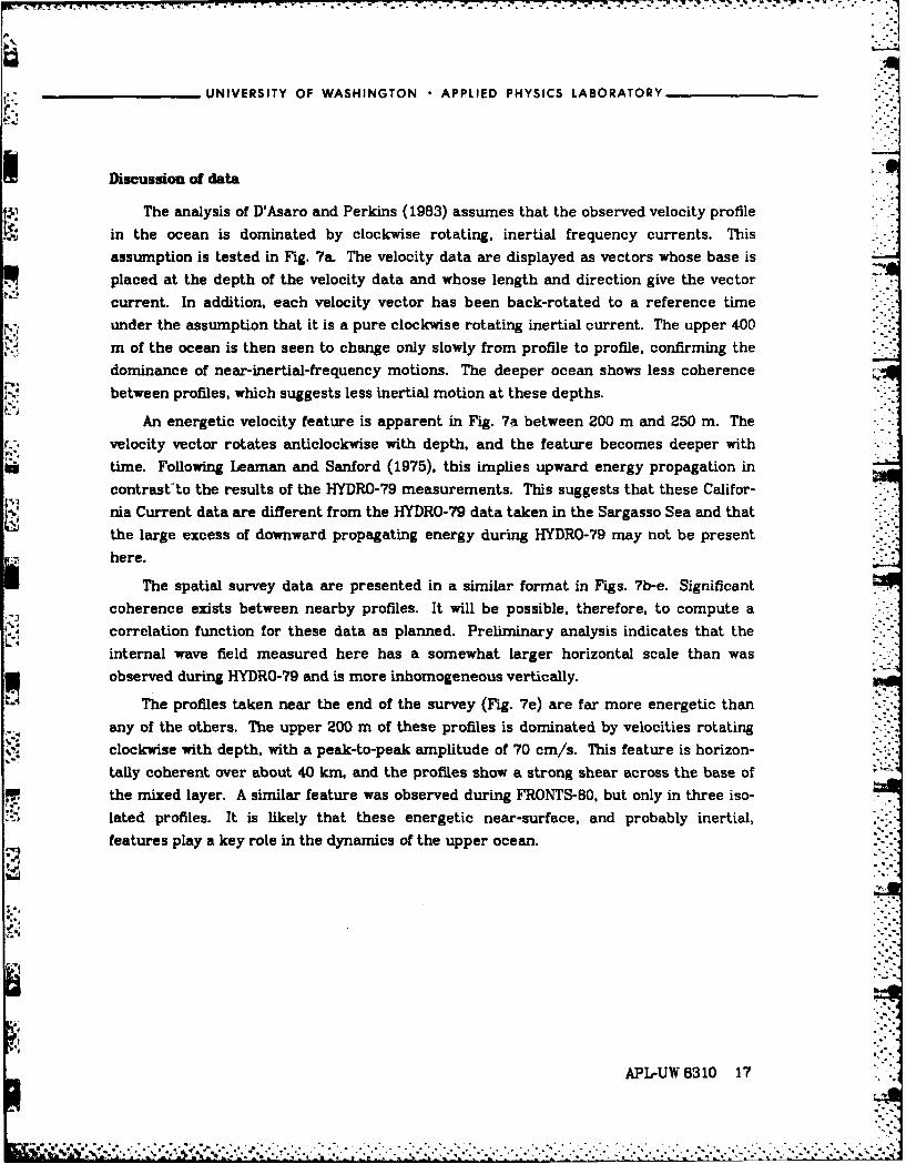
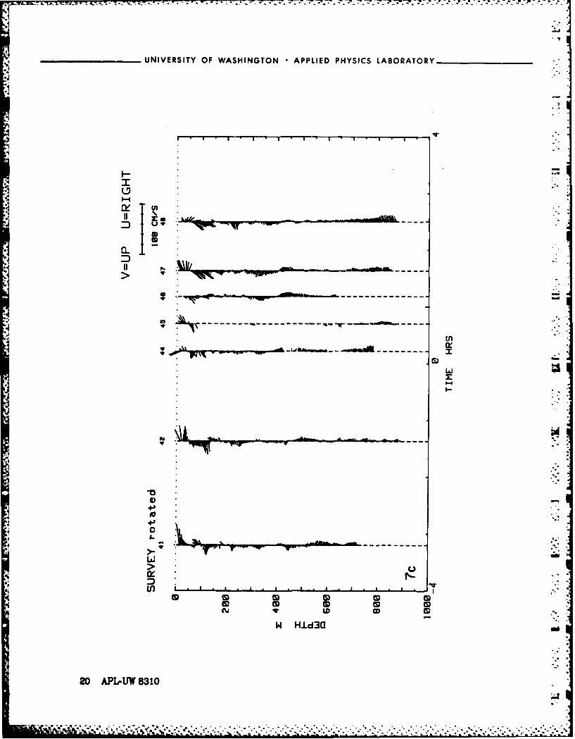
Discussion of data

The analysis of D'Asaro and Perkins (1983) assumes that the observed velocity profile

in the ocean is dominated by clockwise rotating, inertial frequency currents. This

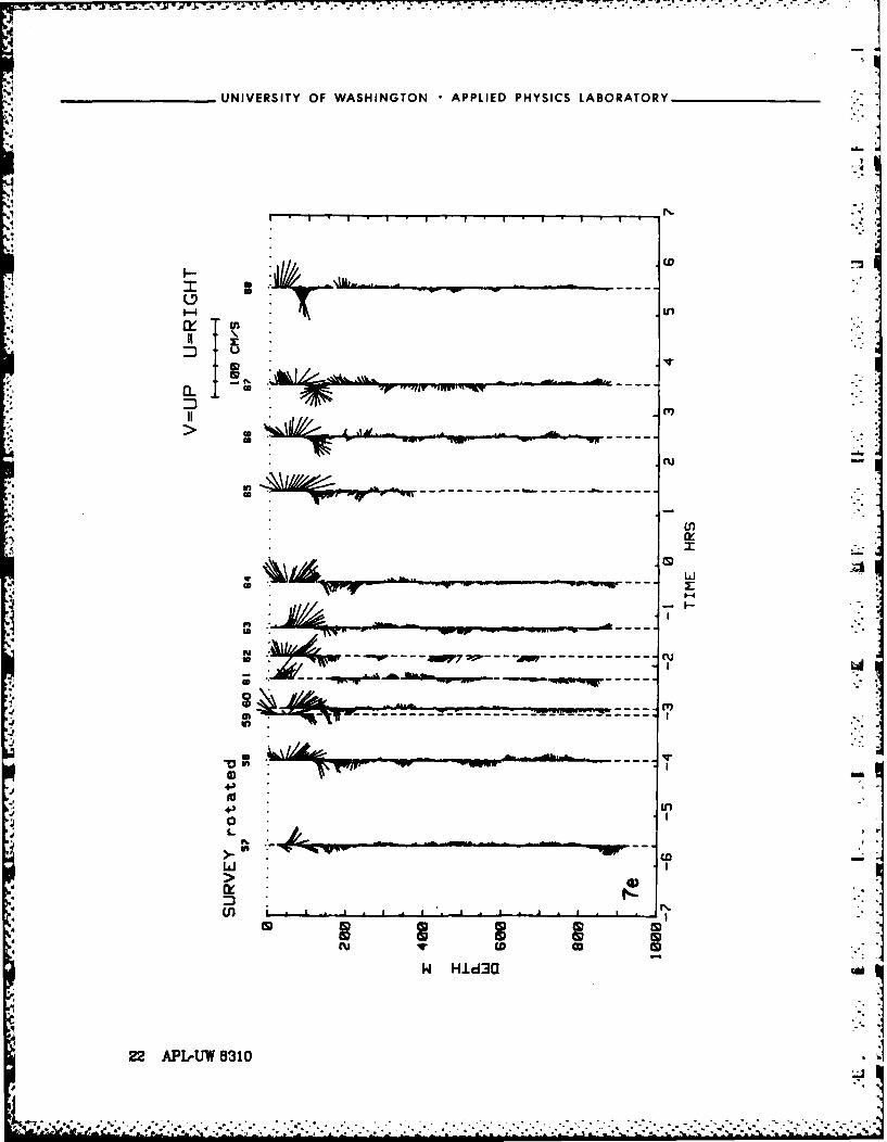
assumption is tested in Fig. 7a. The velocity data are displayed as vectors whose base is

placed at the depth of the velocity data and whose length and direction give the vector

current. In addition, each velocity vector has been back-rotated to a reference time

under the assumption that it is a pure clockwise rotating inertial current. The upper 400

m of the ocean is then seen to change only slowly from profile to profile, confirming the

dominance of near-inertial-frequency motions. The deeper ocean shows less coherence

between profiles, which suggests less inertial motion at these depths.

An energetic velocity feature is apparent in Fig. 7a between 200 m and 250 m. Thevelocity vector rotates anticlockwise with depth, and the feature becomes deeper with

time. Following Leaman and Sanford (1975), this implies upward energy propagation in

contrast-to the results of the HYDRO-79 measurements. This suggests that these Califor-

ia Current data are different from the HYDRO-79 data taken in the Sargasso Sea and that

the large excess of downward propagating energy during HYDRO-79 may not be present

here.

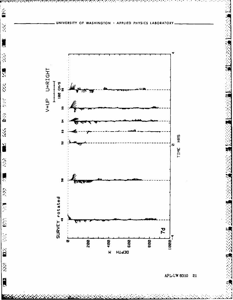
The spatial survey data are presented in a similar format in Figs. 7b-e. Significant

coherence exists between nearby profiles. It will be possible, therefore, to compute a

correlation function for these data as planned. Preliminary analysis indicates that the

internal wave field measured here has a somewhat larger horizontal scale than was

observed during HYDRO-79 and is more inhomogeneous vertically.

The profiles taken near the end of the survey (Fig. 7e) are far more energetic than

any of the others. The upper 200 m of these profiles is dominated by velocities rotating

clockwise with depth, with a peak-to-peak amplitude of 70 cm/s. This feature is horizon-

tally coherent over about 40 kn, and the profiles show a strong shear across the base of

the mixed layer. A similar feature was observed during FRONTS-BO, but only in three iso-

lated profiles. It is likely that these energetic near-surface, and probably inertial,

features play a key role in the dynamics of the upper ocean.

to,

~~~APL-UW 5310 17: .:

-- -w,.. . . .-


"WN ww -

v) w

A_ _ _ _ _ _ _ _ _ _ _ _ _ _ __ _ _ _ _ _ _ _ _ _

'4"o

~c

.CDo

(n

---------------- la

-- -- - -_ _-_---------__ _ _ _ _ _ _

x 0

himw -- -- - 4

0 a

IRM41

QA

w"4i

W Hld3a

18 APL-UW 8310

29~~-' ' *~** 4V* *~. '


ii

>!

ncniir

zm

~~Naswam ------------------------- - -- ---

: L.. -

' 'U

0L

Lii

U) -I% Ir I* I 0 I

N H WO

W Hid~a

APL-UW 8310 19

La6 C - - . * - .. ....

Z. . . . . . . . .- 7- - - - - - -


.L9

F-

*- - - - - - - - - - - - - - -

.11

1 ~ ~Lh~m~mm.~..~pw---------------

I-

W HdA

20~ "L-W 831


UU

> -v

IL

• II• I • l • I • I

-- ---II - -- --

--" " ... r " ....... "" - - - .m I -... . ..

41l

nU,

-o

- 4-

0

L

N.

Li

Cl) - . a -. i . a . . a . I , .

Cu C. DD

W Hid30

APL-UW 8310 21

I


.- 4 . "

I -i

t--- - --cul

nLwtv

xI I

4. . __--o ___-,___...._

-',

• 7p" --- low. . .----------_- __ __.

O ---- ---

. - - . . .. . ------ v

Al

U.°0

4L

-(P

W Hid3a

22 AP-- 8310 .

"'-" "% ' " ' ' -'.' ": .''' , , '. , , -, _', : . , .., ,, : , -. - :,- , '. ' , -. t , ;. "


RECOMMENDATIONS

UTo date, the XCP has been used in several dozen separate measurement programs.

* ... Based on this experience the following recommendations for its future use, particularly

by NORDA. are offered. A distiniction will be made between routine and specializedq oceanographic measurements.

Routine oceanographic measurementsCertain oceanic parameters are sufficiently important to justify an ongoing and con-

tinuous measurement program. Winds and waves are of this nature. Many years of wind

and wave measurements in all oceans from many different ships allow seagoing operations

to be planned anywhere with a general foreknowledge of both the typical and most severewind and wave conditions likely to be encountered. More recently, the various XBT meas-

urement programs have allowed the average thermal structure of the upper ocean to beknown as a function of position and time over much of the ocean. Not only are these data

important for operational purposes, but they also form a vital background for moredetailed oceanographic studies. During 1982, for example, a pool of warm water stretch-ing across the entire equatorial Pacific resulted in a worldwide climatic anomaly called

* "El Nino." The detection of this event was possible only because of the background infor-

mation gathered over many years on upper ocean temperature.

Upper ocea~n shear

The XCP is an ideal instrument for making routine measurements of upper ocean

velocity and shear. These are fundamental characteristics of the upper ocean which are

expected to vary vertically, geographically, and seasonally primarily because of variationsin the internal wave field. The evidence to date suggests enhanced shear at the mixed

layer base and enhanced shear and energy levels during stormy conditions, at particular

locations within fronts, eddies, and major currents such as the Gulf Stream, and near cer-

tain topographic features such as submarine canyons. The extent of these variations, and*. associated variations in upper ocean Richardson number and mnicrostructure, is largely

unknown and will be determined only through a continuing measurement program.

4.. The development of an XCP measurement program designed to characterize the vari-ation of upper ocean shear, velocity, and Richardson number is recommended. Such a

prga ol mlysm obnto fddctdsis hp fopruiy rar

APL-UW 8310 23

- _, . . . .- '-- -- ""


of XCP's with the separation between drops large compared to the coherence distance of

the internal waves. Based on present data, separations of 100 km in the North Pacific and

40 km in the Sargasso Sea would be appropriate. Shorter separations would be used when

potentially significant oceanographic features such as fronts, Gulf Stream rings, or

seamounts were crossed. XBT drops, with a considerably closer spacing, would be used to

detect any unexpected mesoscale features. On scientific vessels, this pattern should be

supplemented with CTD casts. When more sophisticated expendable instruments such as

the XCTD and XDP (Expendable Dissipation Probe) become available, these should be

employed in addition to the XCP.

Eddy monitoring

The XCP can also be an important tool in the routine measurement of low frequency,

geostrophic motions. At present, the major current and eddy systems off the western

coasts of North America and Japan are monitored only through remotely sensed sea sur-

face temperature and occasional XBT's. Present remote sensing techniques accurately

locate oceanographic features, such as Gulf Stream rings, but give little indication of

their strength. More sophisticated remote sensing capabilities, such as satellite

altimetry, promise to give surface geostrophic currents, but will still not measure the

vertical variation in current. The XCP, especially when combined with other techniques,

offers the opportunity for monitoring these current systems throughout the upper ocean.Jn regions of strong low frequency motion, the high frequency, internal wave velocities are

much less energetic, and generally of smaller vertical scale, than the low frequency

motions. Thus, although a single XCP cast measures the sum of the low frequency, geos-

trophic and high frequency, internal wave velocity profiles, a low order polynorrial fit to

the XCP velocity profile generally measures the low frequency velocity profile to within

about 5 cm/s. Used in this way, the XCP can replace CTD computations of dynamic height

as a method for obtaining relative velocity profiles.

The XCP would allow the creation of a routine program to monitor energetic eddy

regions. Such a program could employ either shipborne or airborne XCP's and function

simultaneously as a part of the upper ocean shear program outlined above. Remote sons-

ing would be used to direct a ship or plane to a previously identified feature, a Gulf

Stream ring for example. A section of XCP's would then be made across the ring. Thiswould be done for many different features over time, resulting in a continuous record of

the strength of the strong mesoscale features in the operational area.

-U"44

24 APL-UW 8310

2 .. . . .


Specialized scientific measurements

Velocity is a basic oceanographic variable that is difficult, to measure from a ship.The XCP provides this capacity and therefore has a great many applications in oceano-graphic research. In particular, the XCP has been shown to be a.useful tool in internalwave studies, such as the one described in this report. Opportunities for future internal

* wave research using the XCP include:

(1) Oceanic response to strong storms, both midlatitude cyclones and hurricanes.This is probably best done using AXCP's, both because of their mobility, whichallows the measurements to be placed optimally with relation to the storm,

* .. ~.and because they are less affected by the high sea states within storms thanship-launched XCP's.

*(2) Internal wave interaction with low frequency flows. Present evidence suggestsCb a strong transfer of energy between mean flows and internal waves whose mag-

nitude is important for the dynamics of both. The details of this interactionare not well known and deserve further investigation. In addition, it isexpected that spatially varying mean flows will greatly modify the generation

of internal waves by topography or wind.

(3) Internal wave interaction with topography. Both theory and observation sug-

g est enhanced generation and dissipation of internal waves on topographic* -*,features, especially in the presence of a low frequency flow.

The sampling strategy for investigating these subjects will depend on the goals of aparticular measurement program. However, a mix of spatial and temporal measure-ments such as those described in this report will probably be used in a great many cases.The design elements outlined in this report are likely to be useful in such future measure-ments.

APL-UW 8310 25

________________UNIVERSITY O)F WASHINGTON APPLIED PHYSICS LABORATORY

D'Asaro, E.A., 1983: Wind forced internal waves in the North Pacific and Sargasso Sea.

* (Submitted to J. Phyjs. Ocecmogr.)

D'Asaro, E.A.. and H.T. Perkins. 1983: The spectrum of near-inertial waves in the late sum-

mer Sargasso Sea. (In preparation)

Leaman. KD.. and T.B. Sanford, 1975: Vertical energy propagation of inertial waves: a

- vector spectral analysis of velocity profiles. J1. Ceophys. Res., 80(15). 1975-1978.

Sanford. T.B.. R.G. Drever. J.H. Dunlap, and E.A. D'Asaro. 1982: Design, operation and per-

formnance of an Expendable Temperature and Velocity Profiler (XTVP), APL-UW 8110,

* Applied Physics Laboratory. University of Washington. Seattle. WA.

26 APLUW 831

SECURITY CLASSIFICATION OF THIS PAGE eWhen Date Entered)

REPORT DOCUMENTATION PAGE READ INSTRUCTIONS

**.. 1 REPORT NUMBER 2. GOVT ACCESSION NO. 3 RECIPIENT'S CATALOG NUMBER' [1AD-8/S330,513 4. TITLE (end Subtitle) S. TYPE OF REPORT & PERIOD COVERED

•* XCP MEASUREMENTS OFF CALIFORNIA IN OCTOBER" 1982: CRUISE REPORT AND PRELIMINARY RESULTS Final Report

6. PERFORMING ORG. REPORT NUMBER

APL-UW 83107. AUTHOR(s) S. CONTRACT OR GRANT NUMBER(&)

Eric A. DAsaro N00014-82-C-0038

9. PERFORMING ORGANIZATION NAME AND ADDRESS 10. PROGRAM ELEMENT. PROJECT, TASK

..-. Applied Physics Laboratory, U. of Washington AREA WORK UNIT NUMERS

-. 1013 N.E. 40th StreetSeattle, Washington 98105

It. CONTROLLING OFFICE NAME AND ADDRESS 12. REPORT DATE

Naval Ocean Research and Development Activity August 1983NSTL Station, Mississippi 39529 Is. NUMUEROF PAGES26

14 MONITORING AGENCY NAME & ADDRESS(l diffrent from Controlling Office) IS. SECURITY CLASS. (of thle report)

' e 1So.DECLASSIFICATION DOWNGRADING

16. DISTRIBUTION STATEMENT (of this Report)

i Approved for public release.

17. DISTRIBUTION STATEMENT (of the abstract entered in Block 20. If different from Report)

IS. SUPPLEMENTARY NOTES

1t. KEY WORDS (Continue on revereD eide if noceeeavy aid identify by block number)

. California Current, upper ocean, internal waves, inertial waves, currents,velocity profiling

mS

20. ASSTRACT (Conttinue an reverse side If necessary and identify by block number)

Sixty-nine profiles of horizontal velocity and temperature from thesurface to about 800 m were made using the Expendable Current Profiler(XCP) during De Steiguer cruise 1212, 7-18 October 1982. The XCP's were

kil deployed in a 6 day time series behind a drogued buoy and in a 275 n.mi.zigzag spatial survey. Satellite infrared images were used to locate acruise area away from strong mesoscale features. The measurements weredesigned to estimate the horizontal coherence function of the near-inertial

DD ~ 1473 EDTO OFINV65I 1SOiLgTs0

F ' 4 S/N 0102.LF .014-6601

SECURITY CLASSIFICATION OF TmIS PAGE (ihen Date Entered)

SECURITY CLASSIFICATION OF THIS PAGE(When Data Entered)

frequency internal wave field for comparison with similar measurementsmade in the Sargasso Sea. It was found that the near-inertial wavesare a dominant feature of the velocity field. Significant coherence i1

exists between nearby profiles. It will, therefore, be possible tocompute a correlation function for these data as planned. A near-surfacefeature with peak-to-peak velocities of 70 cm/s was observed and partiallysurveyed.

-- A

.4-

a

SI-.

.. ,

'.

,

2-a

'

"u- •.SEC'URITY CLASSIFeICATION OP' THIS PACE 'flef Date Entaned) a-

" 'bO, e -¢ ,. ,;. .:*.*,.. *.*' .-.-. '."... *.- .--.- -., .-.. .. -- ,.-,2..-... .--- :'---.----?--, . -7-'.---2.-

Date post:	02-Mar-2019
Category:	Documents
Upload:	hathuy
View:	215 times
Download:	0 times

XCP MEAlSUREMENTS OFF CALIFORNIA IN CRUISE · dred CTD and AMP 1 profiles of temperature and...

Documents