XI.Estimation of linear model parameters. XI.A Linear models for designed experiments XI.B Least squares estimation of the expectation parameters in simple linear models XI.C Generalized least squares (GLS) estimation of the expectation parameters in general linear models - PowerPoint PPT Presentation
130
Statistical Modelling Chapter XI 1 XI. Estimation of linear model parameters XI.A Linear models for designed experiments XI.B Least squares estimation of the expectation parameters in simple linear models XI.C Generalized least squares (GLS) estimation of the expectation parameters in general linear models XI.D Maximum likelihood estimation of the expectation parameters XI.E Estimating the variance
Transcript
Statistical Modelling Chapter XI 1
XI. Estimation of linear model parameters
XI.A Linear models for designed experiments
XI.B Least squares estimation of the expectation parameters in simple linear models
XI.C Generalized least squares (GLS) estimation of the expectation parameters in general linear models
XI.D Maximum likelihood estimation of the expectation parameters
XI.E Estimating the variance
Statistical Modelling Chapter XI 2
XI.A Linear models for designed experiments
• In the analysis of experiments, the models that we have considered are all of the form
2 and var i iE Y X Y V S• where
– is an n1 vector of expected values for the observations,– Y is an n1 vector of random variables for the observations,– X is an nq matrix with nq,– is a q1 vector of unknown parameters,– V is an nn matrix,– is the variance component for the ith term in the variance
model and – Si is the summation matrix for the ith term in the variance model.
2i
• Note that generally the X matrices contain indicator variables, each indicating the observations that received a particular level of a (generalized) factor.
Statistical Modelling Chapter XI 3
Summation matrices
1 so that i i
ni i i in f fM S S M
• Si is the matrix of 1s and 0s that forms the sums for the generalized factor corresponding to the ith term.
• Now,
• where – Mi is the mean operator for the ith term in the variance model, – n is the number of observational units and – fi is the number of levels of the generalized factor for this term.
• For equally-replicated, generalized factors n/fi gi where gi is the no. of repeats of each of its levels.
• Consequently, the Ss could be replaced with Ms.
Statistical Modelling Chapter XI 4
For example, variation model with Blocks random for RCBD with b 3 and t 4
Thus the model is of the form:
Block I II III
Unit 1 2 3 4 1 2 3 4 1 2 3 4
1 2BU 2
B
2B 2
B 2B 0 0 0 0 0 0 0 0
2 2B 2
BU 2B
2B 2
B 0 0 0 0 0 0 0 0
3 2B 2
B 2BU 2
B
2B 0 0 0 0 0 0 0 0
4 2B 2
B 2B 2
BU 2B
0 0 0 0 0 0 0 0
1 0 0 0 0 2BU 2
B
2B 2
B 2B 0 0 0 0
2 0 0 0 0 2B 2
BU 2B
2B 2
B 0 0 0 0
3 0 0 0 0 2B 2
B 2BU 2
B
2B 0 0 0 0
4 0 0 0 0 2B 2
B 2B 2
BU 2B
0 0 0 0
1 0 0 0 0 0 0 0 0 2BU 2
B
2B 2
B 2B
2 0 0 0 0 0 0 0 0 2B 2
BU 2B
2B 2
B
3 0 0 0 0 0 0 0 0 2B 2
B 2BU 2
B
2B
4 0 0 0 0 0 0 0 0 2B 2
B 2B 2
BU 2B
T
2 2BU Bn b t
E
Y X
V I I J
note n b bt b t
BU
1B
Now and n
b tt
M I
M I J
2 2BU BU B B
2 2BU BU B B
so t
V M M
S S
Statistical Modelling Chapter XI 5
Classes of linear models• Firstly, linear models split into
– expectation model is of full rank– expectation model is of less than full rank.
• The rank of an expectation model is given by the following definitions — 2nd is equivalent to that given in chapter I.
• Definition XI.1: The rank of an expectation model is equal to the rank of its X matrix.
• Definition XI.2: The rank of an n q matrix X, with n q, is the number of linearly independent columns in X.
• Such a matrix is of full rank when its rank equal q and is of less than full rank when its rank is less than q.
• It will be less than full rank if the linear combination of some columns is equal to the same linear combination as some other columns.
Statistical Modelling Chapter XI 6
Simple vs general models• Secondly, linear models split into those for which
the variation model is – simple in that it is of the form 2In
– more general form that involves more than one term.• For general linear models, S matrices in variation
model can be written as direct products of I and J matrices.
Definition XI.3: The direct-product operator is denoted and, if Ar and Bc are square matrices of order r and c, respectively, then
11 1
1
r
r c
r rr
a a
a a
B BA B
B B
Statistical Modelling Chapter XI 7
Expressions for S matrices in general models
• When all the variation terms correspond to only unrandomized, and not randomized, generalized factors, use the following rule to derive these expressions.
• Rule XI.1: The Si for the ith generalized factor from the unrandomized structure that involves s factors, is the direct product of s matrices, provided the s factors are arranged in standard order.
• Taking the s factors in the sequence specified by the standard order, – for each factor in the ith generalized factor include an I matrix in
the direct product and – J matrices for those that are not. – The order of a matrix in the direct product is equal to the number
of levels of the corresponding factor.
Statistical Modelling Chapter XI 8
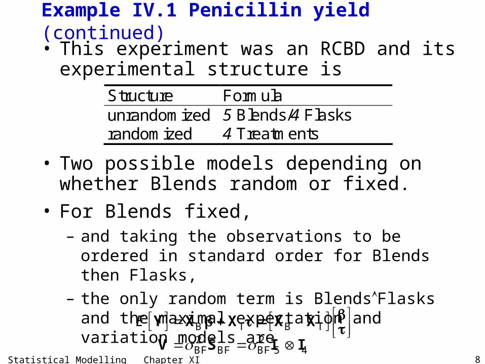
Example IV.1 Penicillin yield (continued)
• This experiment was an RCBD and its experimental structure is
Structure Formula unrandomized 5 Blends/4 Flasks randomized 4 Treatments
• Two possible models depending on whether Blends random or fixed.
• For Blends fixed, – and taking the observations to be ordered in standard
order for Blends then Flasks, – the only random term is BlendsFlasks and the
maximal expectation and variation models are
B T B TE Y X X X X
2 2BF BF BF 5 4 V S I I
Statistical Modelling Chapter XI 9
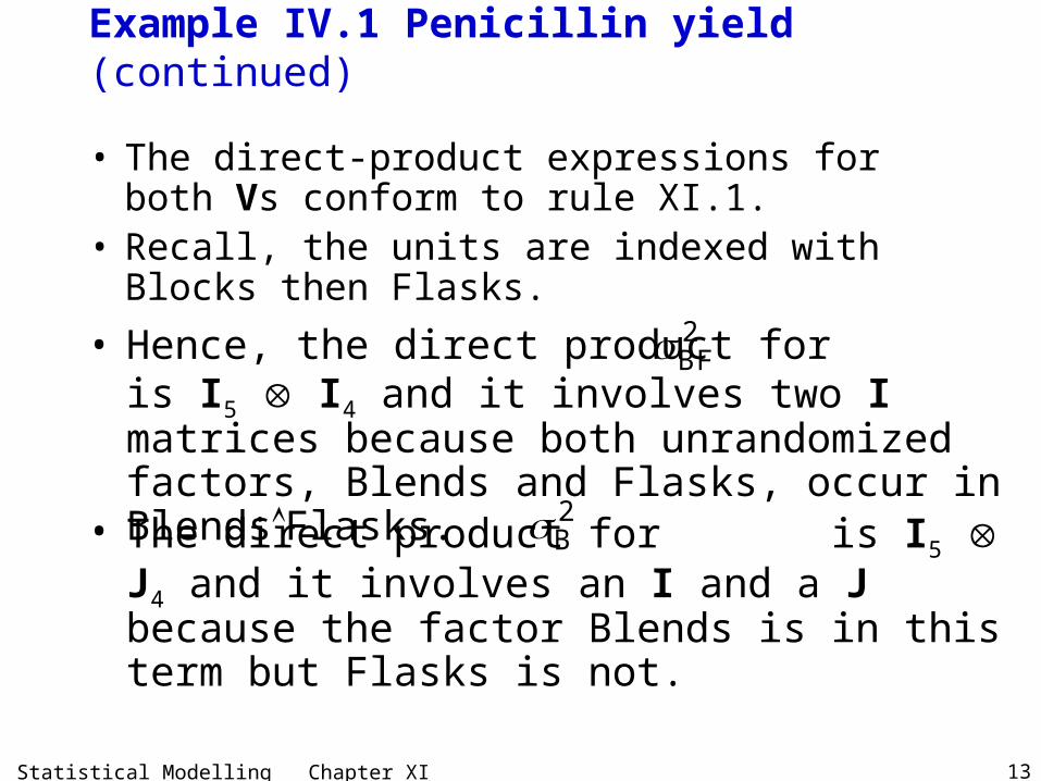
Example IV.1 Penicillin yield (continued)
– Then the vectors and matrices in the
maximal expectation model
are:
B T
B T
E
Y X X
X X
– Suppose observations are in standard order for Blend then Treatment; with Flask renumbered within Blend to correspond to Treatment
as in the prerandomization layout.– Analysis for prerandomization and randomized layouts must be same
as prerandomization layout is one of the possible randomized arrangements.
Example IX.1 Production rate experiment (revisited)• Now if the observations are arranged in standard order
with respect to the factors Factories, Areas and then Parts, we can use rule XI.1 to obtain the following direct-product expression for V.
2 2 2FAP FAP FA FA F F
2 2 2FAP 4 3 3 FA 4 3 3 F 4 3 3.
V S S S
I I I I I J I J J
• So this model allows for – covariance between parts from the same area and – a different covariance between areas from the same factory.
• In this matrix – will occur down the diagonal,
– will occur in 3 3 blocks down the diagonal and – will occur in 9 9 blocks down the diagonal.
2FAP2FA2F
Statistical Modelling Chapter XI 17
Example IX.1 Production rate experiment (revisited)• Actually, in ch. IX, Factories was assumed fixed and so
2 2FAP FAP FA FA
2 2FAP 4 3 3 FA 4 3 3.
V S S
I I I I I J
• So the rules still apply as terms in V only involve unrandomized factors
• This model only allows for – covariance between parts from the same area.
FE MSY X δ X αβ
Statistical Modelling Chapter XI 18
XI.B Least squares estimation of the expectation parameters in simple linear models
• Want to estimate the parameters in the expectation model by establishing their estimators.
• There are several different methods for doing this.
• A common method is the method of least squares, as in the following definition originally given in chapter I.
Statistical Modelling Chapter XI 19
a) Ordinary least squares estimators for full-rank expectation models
• Definition XI.4: Let Y X + where– X is an nq matrix of rank m q with nq, – is a q1 vector of unknown parameters, – is an n1 vector of errors with mean 0 and variance 2In.
The least ordinary least squares (OLS) estimator of is the value of that minimizes
21
nii ε ε
• Note applies to the less-than-full rank case
Statistical Modelling Chapter XI 20
Least squares estimators of • Theorem XI.1: Let Y X + where
– Y is an n1 vector of random variables for the observations, – X is an nq matrix of full rank with nq, – is a q1 vector of unknown parameters, – is an n1 vector of errors with mean 0 and variance 2In.
The ordinary least squares estimator of is given by
1ˆ θ X X X Y
• (The ‘^’ denotes estimator)• Proof: Need to set differential of ' (Y – X)'Y – X)
to zero (see notes for details);• Yields the normal equations whose solution
is given above.ˆ X Xθ X Y
Statistical Modelling Chapter XI 21
Estimator of • Using definition I.7 (expected values), an estimator of
the expected values is
1ˆˆ ψ Xθ X X X X Y• Now for experiments
– the X matrix consists of indicator variables and – the maximal expectation model is generally the sum of
terms each of which is an X matrix for a (generalized) factor and an associated parameter vector.
• In cases where maximal expectation model involves a single term corresponding to just one generalized factor, – the model is necessarily of full rank and – the OLS estimator of its parameters is particularly
simple.
Statistical Modelling Chapter XI 22
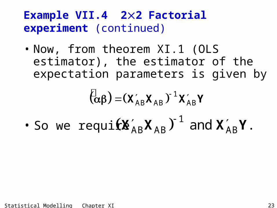
Example VII.4 22 Factorial experiment• To aid in proofs coming up consider a two-factor factorial
experiment (as in chapter 7, Factorial experiments).• Suppose there are the two factors A and B with a b
2, r 3 and n 12. • Assume that data is ordered for A then B then replicates.
Proofs for expected values for a single-term model
• First prove that model is of full rank and then derive the OLS estimator.
• Lemma XI.1: Let X be an n f matrix with n ≥ f.
Then rank(X) rank(XX).
Proof: not given.
Statistical Modelling Chapter XI 29
Proofs for expected values for a single-term model (continued)
• Lemma XI.2: Let Y X + where X is an n f matrix corresponding to a generalized factor, F say, with f levels and n ≥ f. Then, the rank of X is f so that X is of full rank.
• Proof: Lemma XI.1 states that rank(X) rank(XX) and it is easier to derive the rank of XX.
• To do this we need to establish a general expression for XX which we do by considering the form of X.
Statistical Modelling Chapter XI 30
Proofs for expected values for a single-term model (continued)• Now
– n rows of X correspond to observational units in the experiment and
– f columns to the levels of the generalized factor.
• All the elements of X are either 0 or 1 – In the ith column, a 1 occurs for those units with the ith
level of the generalized factor so that, if the ith level of the generalized factor is replicated gi times, there will be gi 1s in the ith column.
– In each row of X there will be a single 1 as only one level of the generalized factor can be observed with each unit if it is the ith level of the generalized factor that occurs on the unit, then the 1 will occur in the ith column of X.
Statistical Modelling Chapter XI 31
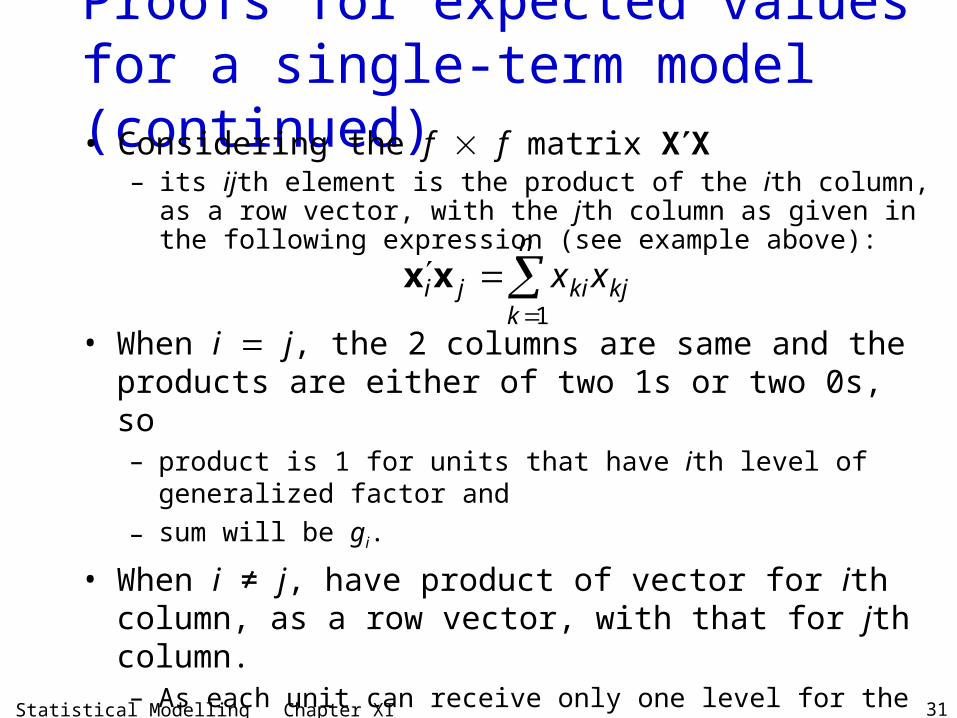
Proofs for expected values for a single-term model (continued)• Considering the f f matrix XX
– its ijth element is the product of the ith column, as a row vector, with the jth column as given in the following expression (see example above):
• When i j, the 2 columns are same and the products are either of two 1s or two 0s, so – product is 1 for units that have ith level of generalized factor and
– sum will be gi.
• When i ≠ j, have product of vector for ith column, as a row vector, with that for jth column. – As each unit can receive only one level for the generalized factor,
it cannot receive both ith and jth levels and the products are either two 0s or a 1 and a 0.
– Consequently, sum is zero.
1
n
i j ki kjk
x x
x x
Statistical Modelling Chapter XI 32
Proofs for expected values for a single-term model (continued)
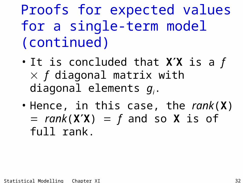
• It is concluded that XX is a f f diagonal matrix with diagonal elements gi.
• Hence, in this case, the rank(X) rank(XX) f and so X is of full rank.
Statistical Modelling Chapter XI 33
Proofs for expected values for a single-term model (continued)• Theorem XI.2: Let Y X +
where – X is an n f matrix corresponding to a generalized
factor, F say, with f levels and n ≥ f.– is a f 1 vector of unknown parameters, – is an n1 vector of errors with mean 0 and variance 2In.
The ordinary least squares estimator of is denoted by and is given by θ
1ˆ
fθ F
where is the f-vector of means for the levels of the generalized factor F.
1fF
double over-dots indicate not n-vector, but f-vector.
Statistical Modelling Chapter XI 34
Proofs for expected values for a single-term model (continued)
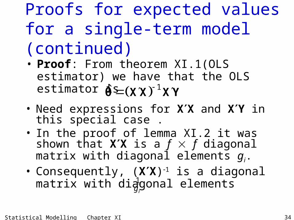
• Need expressions for XX and XY in this special case .
• In the proof of lemma XI.2 it was shown that XX is a f f diagonal matrix with diagonal elements gi.
• Proof: From theorem XI.1(OLS estimator) we have that the OLS estimator is
1ˆ θ X X X Y
• Consequently, (XX)1 is a diagonal matrix with diagonal elements 1
ig
Statistical Modelling Chapter XI 35
Proofs for expected values for a single-term model (continued)• Now XY is an f-vector whose ith element is the
total for the ith level of the generalized factor of the elements of Y. – This can be seen when it is realized that the ith
element of XY is the product of the ith column of X with Y.
– Clearly, the result will be the sum of the elements of Y corresponding to elements of the ith column of X that are one:
those units with the ith level of the generalized factor.
• Finally, taking the product of (XX)1 with XY divides each total by its replication forming the f-vector of means as stated.
Statistical Modelling Chapter XI 36
Proofs for expected values for a single-term model (continued)• Corollary XI.1: With the model for Y as in
theorem XI.2, the estimator of the expected values are given by
1 Fˆˆ n ψ Xθ F M Y
where– is the n-vector an element of which is the
mean for the level of the generalized factor F for the corresponding unit and
– MF is the mean operator that replaces each observation in Y with the mean for the corresponding level of the generalized factor F.
1nF
Statistical Modelling Chapter XI 37
Proofs for expected values for a single-term model (continued)• Proof: Now and, as stated in proof of
lemma XI.2 (rank X), each row of X contains a single 1 – if it is the ith level of the generalized factor that occurs
on the unit, then the 1 will occur in the ith column of X.
ˆˆ ψ Xθ
• To show that , we have from theorem XI.1 (OLS estimator) that
Fˆ ψ M Y 1ˆˆ ψ Xθ X X X X Y
• Now, given also, MF must be the mean operator that replaces each observation in Y with the mean for the corresponding level of the F.
1ˆ nψ F
• So corresponding element of will be the ith element of which is the mean for the ith level of the generalized factor F and
1ˆ
fθ F
1ˆ nψ F
ˆˆ ψ Xθ
• Letting yields 1F
X X X X M Fˆ ψ M Y
Statistical Modelling Chapter XI 38
Example XI.1 Rat experiment
• See lecture notes for this example that involves a single, original factor whose levels are unequally replicated.
Statistical Modelling Chapter XI 39
b) Ordinary least squares estimators for less-than-full-rank expectation models
• The model for the expectation is still of the form E[Y] X but in this case the rank of X is less than the number of columns.
• Now rank(X) rank(XX) m < q and so there is no inverse of XX to use in solving the normal equations
ˆ X Xθ X Y
B+Tˆ ψ B T G
• Our aim is to show that, in spite of this and the difficulties that ensue, the estimators are functions of means.
• For example, the maximal, less-than-full-rank, expectation model for an RCBD is:
B+T E[Y] XBXT
• Will show, with some effort, the estimator of the expected values is:
Statistical Modelling Chapter XI 40
Less-than-full-rank vs full-rank model1. In the full rank model it is assumed that the parameters
specified in the model are unique.There exists exactly one set of real numbers {1, 2, …, q} that describes the system.
In the less-than-full-rank model there are infinitely many sets of real numbers that describe the system.
For our example, there are infinitely many choices for {1, …, b, 1, …, t}. The model parameters are said to be nonidentifiable.
3. In the full rank model all linear functions of {1, 2, …, q} can be estimated unbiasedly. In the less-than-full-rank model some functions can while others cannot. Want to identify functions with invariant estimated values.
2. In the full rank model XX is nonsingular and so (XX)1 exists and the normal equations have the one solution:
In a less-than-full-rank model there are infinitely many solutions to the normal equations.
1ˆ X X X Y
Statistical Modelling Chapter XI 41
Example XI.2 The RCBD
• Simplest model that is less than full rank is the maximal expectation model for the RCBD,
E[Y] = Blocks + Treats.• Generally, RCBD involves b blocks with t
treatments so that there are n b t observations.
• The maximal model used for an RCBD, in matrix terms, is:
B+T E[Y] XBXT and var[Y] 2In
• However, as previously mentioned, the model is not of full rank because the sums of the columns of both XB and XT are equal to 1n.
• Consequently, for X [XB XT], rank(X) rank(XX) b + t 1
Statistical Modelling Chapter XI 42
Illustration for b=t=2 that the parameters are nonidentifiable
• Suppose following information is known about the parameters:
1 1
1 2
2 1
2 2
10
15
12
17.
• Then the parameters are not identifiable for:
1.if 1 5, then 1 5, 2 10 and 2 7;
2.if 1 6, then 1 4, 2 9 and 2 8.
• Clearly can pick a value for any one of the parameters and then find values of the others that satisfy the above equations.
• Infinitely many possible values for the parameters.
• However, no matter what values are taken for 1, 2, 1 and 2, the value of 2 1 2 and of 2 - 1 5;
–these functions are invariant.
Statistical Modelling Chapter XI 43
Coping with less-than-full-rank models
• Extend estimation theory presented in section a), Ordinary least squares estimators for full-rank expectation models.
• Involves obtaining solutions to the normal equations using generalized inverses.
Statistical Modelling Chapter XI 44
Introduction to generalized inverses
• Suppose that we have a system of n linear equations in q unknowns such as Ax y
• where– A is an n q matrix of real numbers, – x is a q-vector of unknowns and – y is a n-vector of real numbers.
• There are 3 possibilities:1. the system is inconsistent and has no solution;2. the system is consistent and has exactly one
solution;3. the system is consistent and has many solutions.
Statistical Modelling Chapter XI 45
Consistent vs inconsistent equations• Consider the following equations:
x1 + 2x2 73x1 + 6x2 21
• They are consistent in that the solution of one will also satisfy the second because the second equation is just 3 times the first.
• However, the following equations are inconsistent in that it is impossible to satisfy both at the same time:
x1 + 2x2 73x1 + 6x2 24
• Generally, to be consistent, any linear relations on the left of the equations must also be satisfied by the righthand side of the equation.
• Theorem XI.3: Let E[Y] X be a linear model for the expectation. Then the system of normal equations
is consistent.Proof: not given.
ˆ X X X Y
Statistical Modelling Chapter XI 46
Generalized inverses
• Definition XI.5: Let A be an n q matrix. A q n matrix A such that
AAA = A
is called a generalised inverse (g-inverse for short) for A.
• Any matrix A has a generalized inverse but it is not unique unless A is nonsingular, in which case A A1.
Statistical Modelling Chapter XI 47
Example XI.3 Generalized inverse of a 22 matrix
It is easy to see that the following matrices are also generalized inverse for A:
12 02 0Take , then 0 0 0 0
A A
12 02 0 2 0 2 0since 0 0 0 0 0 00 0
1 12 20 0 and
1 1 4 3
This illustrates that generalized inverses are not necessarily unique.
Statistical Modelling Chapter XI 48
An algorithm for finding generalized inverses
To find a generalized inverse A for an matrix A of rank m:
1. Find any m m minor H of A i.e. the matrix obtained by selecting any m rows and any m columns of A.
2. Find H1.3. Replace H in A with (H1)'.4. Replace all other entries in A with zeros.5. Transpose the resulting matrix.
Statistical Modelling Chapter XI 49
Properties of generalized inverses
• Let A be an n q matrix of rank m with n q m.
• Then1. AA and AA are idempotent.
2. rank(AA) rank(AA) m.
3. If A is a generalized inverse of A, then (A)' is a generalized inverse of A'; that is, (A)' = (A').
4. (A'A)A' is a generalized inverse of A so that A A(A'A)(A'A) and A' (A'A)(A'A)A'.
5. A(A'A)A' is unique, symmetric and idempotent as it is invariant to the choice of a generalized inverse. Furthermore rank(A(A'A)A') m.
Statistical Modelling Chapter XI 50
Generalized inverses and the normal equations
• Lemma XI.3: Let Ax y be consistent. Then x Ay is a solution to the system where A is any generalized inverse for A.
• Proof: not given.
Statistical Modelling Chapter XI 51
• Proof: In our proof for the full-rank case, showed that the LS estimator is the solution of the normal equations.
• Nothing in our derivation of this result depended on the rank of X. – So the least squares estimator in the less-than-full-rank case is
still a solution to the normal equations .
Generalized inverses & the normal equations (cont’d)• Theorem XI.4: Let Y X +
where X is an n q matrix of rank m q with n q, is a q 1 vector of unknown parameters, is an n 1 vector of errors with mean 0 and variance 2In. The ordinary least squares estimator of is denoted by and is given by ˆ . θ X X X Y
θ
ˆ X X X Y• Applying theorem XI.3 (normal eqns consistent) and
lemma XI.3 (g-inverse gives soln) to the normal equations, yields as a solution of the ˆ X X X Ynormal equations as claimed. (not unique — see notes)
Statistical Modelling Chapter XI 53
A useful lemma• Next theorem derives the OLS estimators for the less-
than-full-rank model for the RCBD. • But, first a useful lemma.• Lemma XI.4: The inverse of is
where a and b are scalars.
1 1m m mm m
a b I J J
1 11 1m m mm ma b I J J
• Proof: First show that 21 1 ,m mm mJ J 21 1m m m mm m I J I J
1 1and .m m mm m I J J 0
• Consequently,
1 1 1 1
1 1
1 1m m m m m mm m m m
m m mm m
m
a ba b
I J J I J J
I J J
I
• so that is the inverse of 1 11 1m m mm ma b I J J
1 1m m mm m
a b I J J
Think of J matrices as “sum-everything” matrices.
Statistical Modelling Chapter XI 54
OLS estimators for the less-than-full-rank model for the RCBD• Theorem XI.6: Let Y be a n-vector of jointly-distributed
random variables with E[Y] XB + XT and var[Y] 2In
where – , XB, and XT are the usual vectors and matrices.
• Then a nonunique estimator of , obtained by deleting the last row and column of X in computing the g-inverse,is
1
1 1 1ˆ
0
b t b b
tt t
T Y
T
B 1 1
T 1
where– is the b-vector of block means of Y, – is the (t 1)-vector of the first t 1 treatment means
of Y,– is the mean of Y for treatment t and – is the grand mean of Y.
1bB
1 1t T
YtT
• Triple over-dots indicates a modified, double over-dots vector
• In this case, t-vector modified
1tT
Statistical Modelling Chapter XI 56
Proof of theorem XI.6• According to theorem XI.4 (OLS for LTFR),
• and so we require a generalized inverse of X'X where X [XB XT], so that
An algorithm for finding generalized inverses (from before)
To find a generalized inverse A for an matrix A of rank m:
1. Find any m m minor H of A i.e. the matrix obtained by selecting any m rows and any m columns of A.
2. Find H1.3. Replace H in A with (H1)'.4. Replace all other entries in A with zeros.5. Transpose the resulting matrix.
Statistical Modelling Chapter XI 58
Proof of theorem XI.6
B B B B TB T
T T B T T
b b t
t b t
tb
I JX X X X XX X X XX X X X X J I
• Our algorithm tells us that we must take a minor of order b+t1 and obtain its inverse.
• So delete any row and column and find its inverse – say last row and column.
• To remove the last row and column of X'X, – let Z [XB XT1] where XT1 is the n(t 1) matrix formed by taking
the first t 1 columns of XT.
• Then,
1B B B T 1
T 1 B T 1 T 1 1 1
b b t
t b t
tb
I JX X X XZ Z X X X X J I
is X'X with its last row and column removed.
• Now Z'Z is clearly symmetric so that its inverse will be also. Our generalized inverse will be with a row and column of zeros added. (no need to transpose)
1Z Z
Statistical Modelling Chapter XI 59
Proof of theorem XI.6 (continued)• Now to find the inverse of Z'Z we note that
– for a partitioned, symmetric matrix H where A CH C D
– then
1 1
1 1 1
11 1 .
H H
U VV W
A VC A A CW
WC A D C A C
• In our case
1
1 1
b b t
t b t
tb
I J A CZ Z J I C D
• So first we need to find W, then V and lastly U
Statistical Modelling Chapter XI 60
Proof of theorem XI.6 (continued)
• Note that lemma XI.4 (special inverse) is used to obtain the inverse in this derivation.
11
11
1 1 1
1
1 1
111 1
1 11
11 1 1
1 11
11 1 1 1
1 1 11 1
1 1 11 1 11 1
111 11
11 1
1
.
bt t b b tt
bt tt
tt tb t t
t tb t t
t t tb t t t
t t tb t t
tt tb t
t tb
b
b
t
W D C A C
I J I J
I J
I J
I J
I J J
I J J
I J
I J
1
1 1
b b t
t b t
tb
I JZ Z J I
A CC D
Statistical Modelling Chapter XI 61
Proof of theorem XI.6 (continued)
1
1 1
b b t
t b t
tb
I J A CZ Z J I C D
1
1 11 1 1
11 1
11
1
b b t t tt b
b t b tbt
b tb
t
V A CW
I J I J
J J
J
1 1
1 1 11 1
11 .
b bb t t bt b t
tb bt bt
U A VC A
I J J I
I J
11 111
1 11 1 1 1 1
1 1 1
.0
tb b bb tt bt b
t b t t tb b
b t
I J J 0
X X J I J 00 0
• and
11 1
111 1
1 1 1
tb b b tt bt b
t b t tb b
I J JZ Z
J I J• Consequently,
Statistical Modelling Chapter XI 62
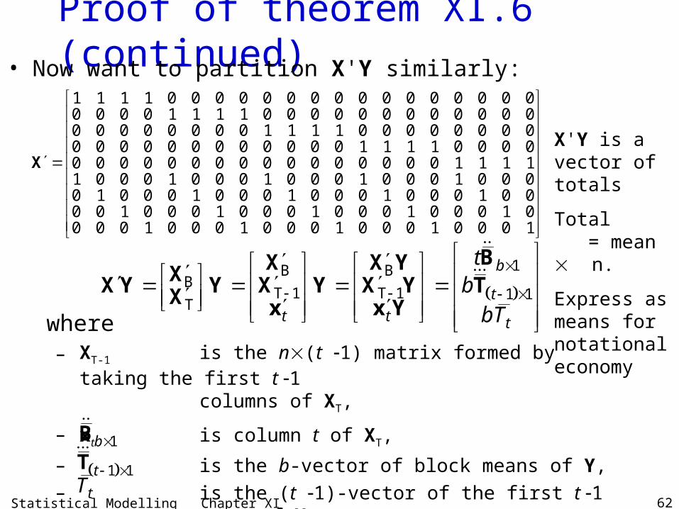
Proof of theorem XI.6 (continued)• Now want to partition X'Y similarly:
where– XT-1 is the n(t 1) matrix formed by taking the first t 1
columns of XT,
– xt is column t of XT,
– is the b-vector of block means of Y, – is the (t 1)-vector of the first t 1 treatment means
of Y,– is the mean of Y for treatment t and
1bB
1 1t T
tT
Statistical Modelling Chapter XI 63
Proof of theorem XI.6 (continued)• Hence the nonunique estimators of are
1 1
11 111 1
1 11 1 1 1 1 1 1
1 1 1
11 1 1 1
11 1 1
ˆ
0
.
0t
tb b bb tt bt b b
t b t t t tb b
b tt
tb b b b t tb
tbt b t tb
tb
bT
X X X Y
I J J 0 BJ I J 0 T0 0
I J B J T
J B I J T
• Now to simplify this expression further we look to simplify
1,b bJ B 11 ,bt b J B 1 1 1,t t J T 1 1 1.b t t J T
Statistical Modelling Chapter XI 64
Proof of theorem XI.6 (continued)• Firstly, each element of is the sum of the b Block
means and 1b bJ B
1 1
b bj jj j
B b B b bY
where is the grand mean of all the observations. Y
• Hence, 1b b bbY J B 1
• Similarly, 11 1bt b tbY J B 1
• Next, each element of is the sum of the first (t 1) Treatment means and
1 1 1t t J T
1
1 1
t ti i t ti i
T T T tY T
• Hence, 1 1 1 1tt t ttY T J T 1
• Similarly, 1 1 1 t bb t t tY T J T 1
Statistical Modelling Chapter XI 65
Proof of theorem XI.6 (continued)• Summary:
1b b bbY J B 1
11 1bt b tbY J B 1
1 1 1 1tt t ttY T J T 1
1 1 1 t bb t t tY T J T 1
• Therefore
11 1 1 1
11 1 1 1 1ˆ
0
tb b b b t tb
tbt b t t tb
I J B J T
J B I J T
1
1 1 1 1
1
1 1 1
1
0
.
0
b b t b
tt t t
b t b b
tt t
t Y tY TtY tY T
T Y
T
B 1 11 T 1
B 1 1
T 1
• So the estimator is a function of block, treatment and grand means, albeit a rather messy one.
Statistical Modelling Chapter XI 66
c) Estimable functions
• In the less-than-full-rank model the problem we face is that cannot be estimated uniquely as it changes for the many different choice of (X'X).
• To overcome consider those linear functions of that are invariant to the choice of (X'X) and hence to the particular obtained.
• This property is true for all estimable functions.
• That is, consider functions whose estimators are invariant to different s in that their values remain the same regardless of which solution to the normal equations is used.
θ ˆθ
Statistical Modelling Chapter XI 67
Definition of estimable functions• Definition XI.6: Let E[Y] X and var[Y] 2In where X
is n q of rank m q. • A function ' is said to be estimable if there exists a vector
c such that E[c'Y] ' for all possible values of .• This definition is saying that, to be estimable, there must
be some linear combination of the random variables Y1, Y2, …, Yn that is a linear unbiased estimator of '.
• In the case of several linear functions, we can extend the above definition as follows:
• If L is a k q matrix of constants, then L is a set of k estimable functions if and only if there is a matrix C of constants so that E[CY] L for all possible values of .
• However, how to identify estimable functions?• The following theorems give us some important cases that
will cover the quantities of most interest.
Statistical Modelling Chapter XI 68
Expected value results
• Lemma XI.5: Let – a be a k 1 vector of constants, – A an s k matrix of constants and – Y a k 1 vector of random variables or
random vector.
and var ;E a a a 0
and var var ;E E a Y a Y a Y a Y a
and var var .E E AY A Y AY A Y A
Statistical Modelling Chapter XI 69
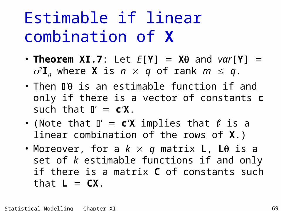
Estimable if linear combination of X
• Theorem XI.7: Let E[Y] X and var[Y] 2In where X is n q of rank m q.
• Then ' is an estimable function if and only if there is a vector of constants c such that ' c'X.
• (Note that ' c'X implies that is a linear combination of the rows of X.)
• Moreover, for a k q matrix L, L is a set of k estimable functions if and only if there is a matrix C of constants such that L CX.
Statistical Modelling Chapter XI 70
Proof• First suppose that ' is estimable. • Then, by definition XI.6 (estimable function),
there is a vector c so that E[c'Y] '. • Now, using lemma XI.5 (E rules) , E[c'Y] c'E[Y] c'X.
• But also E[c'Y] ' and so c'X = '. • Since this last equation is true for all , follows
that c'X = '.• Second, suppose that ' = c'X. • Then ' = c'X = E[c'Y] and, by definition XI.6
(estimable function), ' is estimable.• Similarly, if E[CY] L, CX = L for all and
thus CX = L. • Likewise, if L = CX, then L = CX = E[CY] and
hence L is estimable.
Statistical Modelling Chapter XI 71
Expected values are estimable
• Theorem XI.8: Let E[Y] X and var[Y] 2In where X is n q of rank m q. Each of the elements of X is estimable.
• Proof: From theorem XI.7, L is a set of estimable functions if L = CX.
• We want to estimate X, so that L = X and so to have L = CX we need to find a CX = X Clearly, setting C In we have that CX = X = L and as a consequence X is estimable.
Statistical Modelling Chapter XI 72
A linear combination of estimable functions is itself estimable
• Theorem XI.9: Let be a collection of k estimable functions.
Let be a linear combination of these functions.
Then z is estimable.
1 2, , , k
1 1 2 2 k kz a a a
• Proof: If each of is estimable then, by definition XI.6 (estimable function), there exists a vector of constants ci such that
, 1, , ,i i k θ
i iE c Y θ
• Then
where
and so z is estimable.
1 1 1
k k ki i i i i ii i i
z a a E E a E
θ c Y c Y d Y
1
ki ii
a
d c
Statistical Modelling Chapter XI 73
Finding all the estimable functions
• First find X, all of whose rows are estimable functions.
• It can be shown that all estimable functions can be expressed as a linear combination of the entries in X.
• So find all linear combinations of X and you have all the estimable functions.
Statistical Modelling Chapter XI 74
Example XI.2 The RCBD (continued)
• For the RCBD, the maximal model is E[Y] XB + XT.
• So for b 5, t 4, 1 1
1 2
1 3
1 4
2 1
2 2
2 3
2 4
3 1
3 2
3 3
3 4
4 1
4 2
4 3
4 4
5 1
5 2
5 3
5 4
.
ψ
• From this we identify the 20 basic estimable functions, i + k.
• Any linear combination of these 20 is estimable and any estimable function can be expressed as a linear combination of these.
• Hence i – i' and k – k' are estimable. • On the other hand, neither i nor k + k'
are estimable.
Statistical Modelling Chapter XI 75
d) Properties of estimable functions
• So we have seen what estimable functions are and how to identify them, but why are they important?
• Turns out that they can be unbiasedly and uniquely estimated using any solution to the normal equations and that they are, in some sense, best.
• It is these properties that we establish in this section.
• But first a definition.
Statistical Modelling Chapter XI 76
The LS estimator of an estimable function
• Definition XI.7: Let ' be an estimable function and let be a least squares estimator of .
ˆ θ X X X Y
• Then is called the least squares estimator of '.
ˆθ
• Now the implication of this definition is that is the unique estimator of '.
ˆθ
• This is not at all obvious because there are infinitely many solutions to the normal equations when they are less than full rank.
θ
• The next theorem establishes that the least squares estimator of an estimable function is unique.
Statistical Modelling Chapter XI 77
Recall properties of g-inverses
• Let A be an n q matrix of rank m with n q m.
• Then1. AA and AA are idempotent.
2. rank(AA) rank(AA) m.
3. If A is a generalized inverse of A, then (A)' is a generalized inverse of A'; that is, (A)' = (A').
4. (A'A)A' is a generalized inverse of A so that A A(A'A)(A'A) and A' (A'A)(A'A)A'.
5. A(A'A)A' is unique, symmetric and idempotent as it is invariant to the choice of a generalized inverse. Furthermore rank(A(A'A)A') m.
Statistical Modelling Chapter XI 78
LS estimator of estimable function is unique• Theorem XI.10: Let ' be an estimable function.
Then least squares estimator is invariant to the least squares estimator .
That is, the expression for is the same for every expression for
ˆθθ
ˆθ ˆ θ X X X Y
• Hence is invariant to (X'X) and hence . ˆθ θ
• Proof: From theorem XI.7 (estimable if ' c'X), we have ' c'X and, from theorem XI.4 (LS/LTFR), ˆ θ X X X Y
• Using these results we get that ˆ θ c X X X X Y• Since, from property 5 of generalized inverses,
is invariant to choice of (X'X), it follows that has the same expression for any choice of (X'X).
X X X X c X X X X Y
Statistical Modelling Chapter XI 79
Unbiased and variance
• Next we show that the least squares estimator of an estimable function is unbiased and obtain its variance.
• Theorem XI.11: Let E[Y] X and var[Y] 2In where X is n q of rank m q.
• Then is unbiased for '. • Moreover, , which is
invariant to choice of generalized inverse.
ˆθ
2ˆvar θ X X
• Also let ' be an estimable function and be its least square estimator.
ˆθ
Statistical Modelling Chapter XI 80
Proof of theorem XI.11
ˆ ˆ
since is a matrix of constants
from property 4 of generalized inverses
.
E E
E
θ θ
X X X Y X X X
X X X Xθ
c X X X X Xθ
c Xθ
θ
• Since and ' c'X we have ˆ θ X X X Y
• This verifies that is unbiased for '. ˆθ
Statistical Modelling Chapter XI 81
Proof of theorem XI.11(continued)• Next
22
2
2
2
ˆvar
var
since var var
and var[ ]
using & property 3 of g-inverses
from prope
nn
θ
X X X Y
a Y a Y aX X X I X X X
Y I
c X X X X X X X X c
X X X Xc X X X X X X X X c
c X X X X c
2
rty 4 of g-inverses
as .X X c X
Statistical Modelling Chapter XI 82
Unbiased only for estimable functions
• The above theorem is most important. • This follows from that fact that is not unbiased
for any '.ˆθ
• In general,
which is not necessarily equal to '.
ˆ ˆE E θ θ X X X Xθ
• Thus the case when ' is estimable, and hence
is an unbiased estimator of it, is a very special case.
ˆθ
Statistical Modelling Chapter XI 83
BLUE = Best Linear Unbiased Estimator• Definition XI.8: Linear estimators are estimators of the
form AY, where A is a matrix of real numbers.• That is, each element of the estimator is a linear
combination of the elements of Y. • The unbiased least squares estimator developed here is
an example of a linear estimator with A '(X'X)X'. • Unfortunately, unbiasedness does not guarantee
uniqueness.• There might be more than one set of unbiased estimators
of . • Another desirable property of an estimator is that it be
minimum variance.• Theorem XI.12, the Gauss-Markoff theorem, guarantees
that, among the class of linear unbiased estimators of ', the least squares estimator is the best in the sense that the variances of the estimator, , is minimized.ˆvar
• For this reason the least squares estimator is called the BLUE (best linear unbiased estimator).
Statistical Modelling Chapter XI 84
A result that will be required in the proof of
the Gauss-Markoff theorem • Lemma XI.6: Let U and V be random variables and a and
b be constants. Then
2 2var var var 2 cov ,aU bV a U b V ab U V • Proof:
2
2
2 2
2 22 2
2 2
var
using definition I.5 of the variance
2
2
var var 2 co
aU bV E aU bV E aU bV
E aU E aU bV E bV
aU E aU bV E bVE
aU E aU bV E bV
a E U E U b E V E V
abE U E U V E V
a U b V ab v , .U V
Note that last step uses definitions I.5 and I.6 of the variance and covariance.
Statistical Modelling Chapter XI 85
Gauss-Markoff theorem• Theorem XI.12 [Gauss-Markoff]: Let E[Y] X and
var[Y] 2In where X is n q of rank m q. Let ' be estimable.
• Then the best linear unbiased estimator of ' is where is any solution to the normal equations.
• This estimator is invariant to the choice of .
ˆ
• Proof: Suppose that a'Y is some other linear unbiased estimator of ' so that E[a'Y] '.
• The proof proceeds as follows:1. Establish a result that will be used subsequently.
2. Prove that is the minimum variance estimator by proving that
3. Prove that is the unique minimum variance estimator.
ˆ ˆvar var a Y
ˆ
Statistical Modelling Chapter XI 86
Proof of theorem XI.12
• Firstly, E[a'Y] a'E[Y] a'X, and since also E[a'Y] ', a'X ' for all .
• Consequently, a'X 'this is the result that will be used subsequently.
• Secondly, we proceed to show that
ˆvar var a Y
• Now, from lemma XI.6 (var[aU + bV]), as and a'Y are scalar random variables and is their linear combination with coefficients 1 and –1, we have
ˆˆ a Y
ˆ ˆ ˆvar var var 2cov , a Y a Y a Y
Statistical Modelling Chapter XI 87
Proof of theorem XI.12 (continued)
ˆcov , cov ,
using definition I.6 of the covariance
as and is a scalar
E E E
E
E
E
a Y X X X Y a Y
X X X Y X X X Y a Y a Y
X X X Y X X X Xθ a Y a Xθ
Y X a Y a Xθ
X X X Y Xθ a
E
E
Y Xθ
X X X Y Xθ Y Xθ a
X X X Y Xθ Y Xθ a
2 2
2
var using definition I.4 for
as var
as
ˆvar .
n
X X X Y a V
X X X a Y I
X X a X
θ
(The last step uses theorem XI.11
— LS and var of est. func.)
Statistical Modelling Chapter XI 88
Proof of theorem XI.12 (continued)
• Since, ˆ ˆvar 0, var var a Y a Y
ˆ ˆ ˆvar var var 2cov ,
ˆ ˆvar var 2var
ˆvar var
a Y a Y a Y
a Y
a Y
• So,
• Hence, has minimum variance amongst all linear unbiased estimators.
ˆ
Statistical Modelling Chapter XI 89
Proof of theorem XI.12 (continued)• Finally, to demonstrate that is the only linear unbiased
estimator with minimum variance, we suppose that
ˆ
ˆvar var a Y
• Then and hence is a constant, say c.
ˆvar 0 a Y ˆ a Y
• Since ˆ ˆ, 0E E E E a Y a Y
so that ˆ 0E a Y
• But so thatˆ c a Y ˆE E c c a Y • Now we have that c 0 and so ˆ a Y • Thus any linear unbiased estimator of ' which has
minimum variance must equal . ˆ• So, provided restrict our attention to estimable functions,
our estimators will be unique and BLU.
Statistical Modelling Chapter XI 90
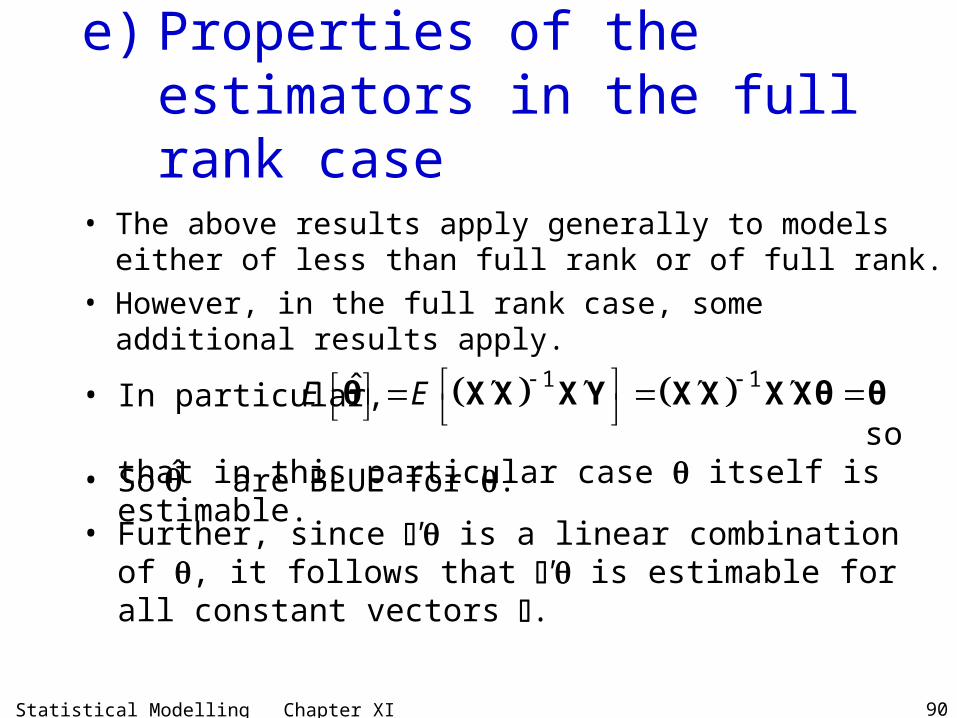
e) Properties of the estimators in the full rank case
• The above results apply generally to models either of less than full rank or of full rank.
• However, in the full rank case, some additional results apply.
• In particular, so that in this particular case itself is estimable.
1 1ˆE E θ X X X Y X X X Xθ θ
• So are BLUE for .
• Further, since ' is a linear combination of , it follows that ' is estimable for all constant vectors .
Statistical Modelling Chapter XI 91
f) Estimation for the maximal model for the RCBD
• In the next theorem, because each of the parameters in ' [' '] is not estimable, we consider the estimators of .– theorem XI.8 tells us that these are estimable, – theorem XI.10 that they are invariant to the
solution to the normal equation chosen and – theorem XI.12 that they are BLUE.
Statistical Modelling Chapter XI 92
Estimator of expected values for RCBD• Theorem XI.13: Let Y be a n-vector of jointly-
distributed random variables with
E[Y] XB + XT and var[Y] 2In
where , XB, and XT are the usual vectors and matrices.
• Then where , and are the n-vectors of block, treatment and grand means, respectively.
ˆ ψ B T G B T G
Statistical Modelling Chapter XI 93
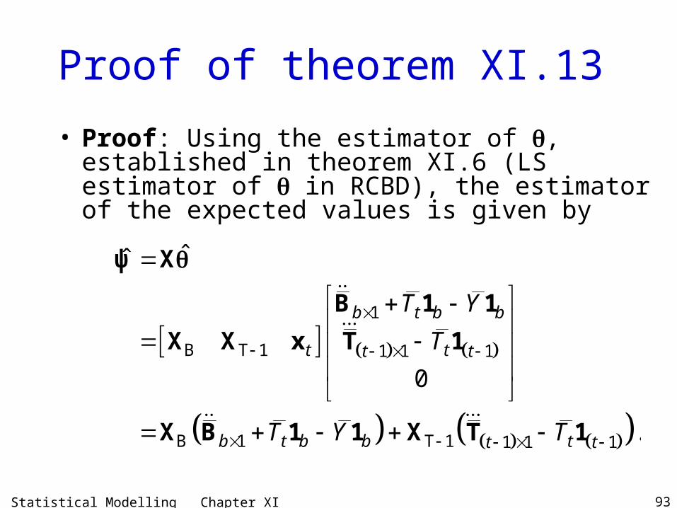
Proof of theorem XI.13
• Proof: Using the estimator of , established in theorem XI.6 (LS estimator of in RCBD), the estimator of the expected values is given by
1
B T 1 1 1 1
B 1 T 1 1 1 1
ˆˆ
0
.
b t b b
t tt t
b t b b tt t
T Y
T
T Y T
ψ X
B 1 1
X X x T 1
X B 1 1 X T 1
Statistical Modelling Chapter XI 94
Proof of theorem XI.13 (continued)1. Now each row of [XB XT1] corresponds to 1 obs:
say obs. in ith block that received jth treat. 2. In the row for obs. in ith block that received jth treat:
– the element in the ith column of XB will be 1, – as will the element in the jth column of XT-1; – all other elements in the row will be zero.
3. Note if treatment is t, only nonzero element will be ith column of XB.
XI.C Generalized least squares (GLS) estimation of the expectation
parameters in general linear models • Define a GLS estimator.• Definition XI.9: Let Y be a random vector with E[Y] X and var[Y] V where X is an n q matrix of rank m q, is a q 1 vector of unknown parameters, V is an n n positive-definite matrix and n q.
• Then the generalized least squares estimator of is the estimator that minimizes the "sum of squares"
1 y X V y X
Statistical Modelling Chapter XI 101
GLS estimator• Theorem XI.14: Let Y be a random vector with E[Y] X and var[Y] V where X is an n q matrix of rank m q, is a q 1 vector of unknown parameters, V is an n n positive-definite matrix and n q.
• Then the generalized least squares estimator of is denoted by and is given by
• Proof: similar to proof for theorem XI.1.
1 1ˆ X V X X V Y
• Unsurprisingly, properties of GLS estimators parallel those for OLS estimators.
• In particular, they are BLUE as the next theorem states.
Statistical Modelling Chapter XI 102
Gauss-Markoff for GLS
• Theorem XI.15 [Gauss-Markoff]: Let Y be a random vector with
E[Y] X and var[Y] V where X is an n q matrix of rank m q, is a q 1 vector of unknown parameters, V is an n n positive-definite matrix and n q. Let ' be an estimable function. Then the generalized least squares estimator
is the best linear unbiased estimator of ', with
• Proof: not given
1 1ˆ X V X X V Y
1ˆvar X V X
Statistical Modelling Chapter XI 103
Estimation of fixed effects for the RCBD when Blocks are random
• We now derive the estimator of in the model for the RCBD where Blocks are random.
• Symbolically, the model is E[Y] = Treats and var[Y] = Blocks + BlocksUnits.
• One effect of making Blocks random is that the maximal, marginality-compliant model for the experiment is of full rank and so the estimator of will be BLUE.
• Before deriving estimators under this model, we establish the properties of a complete set of mutually-orthogonal idempotents as they will be useful in proving the results.
Statistical Modelling Chapter XI 104
Complete set of mutually-orthogonal idempotents
• Definition XI.10: A set of idempotents {QF: F } forms a complete set of mutually-orthogonal idempotents (CSMOI) if
F F F F FF F FF for all F,F and n
Q Q Q Q Q Q IF
F
• Of particular interest is that the set of Q matrices from a structure formula based on crossing and nesting relationships forms a CSMOI.
• e.g. RCBD
where and otherwise.FF 1 if F F' FF 0
Statistical Modelling Chapter XI 105
Inverse of CSMOI• Lemma XI.7: For a matrix that is the linear
combination of a complete set of mutually-orthogonal matrices, such as ,its inverse is
F FF
V Q
F
1 -1F FF
V Q
F• Proof:
1 -1F F F FF F
-1F F F FF F
-1F F F FF
FF
.n
VV Q Q
Q Q
Q Q
Q
I
F F
F F
F
F
Statistical Modelling Chapter XI 106
Estimators for only Treatments fixed• In the following theorem we show that the GLS estimator for the
expectation model when only Treatments is fixed is the same as the OLS estimator for a model involving only fixed Treatments, such as would occur with a CRD.
• However, first a useful lemma.• Lemma XI.8: Let A, B, C and D be square matrices and a, b and c
be scalar constants. Then,
A B C D AC BD
.
a a
a b ab
b c b c
trace trace trace
A B A B
A A
A B A B
A B C A B A C
A B A B
provided A and C, as well as B and D, are conformable.
Statistical Modelling Chapter XI 107
Estimators for only Treatments fixed (cont’d)
• Theorem XI.16: Let Y be an random vector for the observations from an RCBD with the Yijk arranged such that those from the same block occur consecutively in treatment order as in a prerandomized layout.
• Also, let Τ b tE Y X 1 I
2 2 2 2B B BU BU B BUb t b t V S S I J I I
• Then the generalized least squares estimator of is given by 11 1 1
T T T Tˆ b
X V X X V Y X Y
and the GLS estimator of the expected values iswhere
1 TnT M Y 1
T T T T T M X X X X
Statistical Modelling Chapter XI 108
Proof of theorem XI.16• From theorem XI.14 (GLS estimator), the GLS
estimator of is given by
11 1T T Tˆ
X V X X V Ythe generalized inverse being replaced by an inverse here because XT is of full rank.
• To prove the second part of the result, we i. derive an expressions for V1, ii. use this to obtain , iii. invert the last result, and iv. show that
1T T
X V X
11 1 1T T T Tb
X V X X V Y X Y
Statistical Modelling Chapter XI 109
Proof of theorem XI.16 (continued)• We start by obtaining an expression for V in terms of QG,
QB and QBU as these form a complete set of mutually orthogonal idempotents.
• Now, 2 2 2 2B B BU BU B B BU BUt V S S M M
• But, from section IV.C, Hypothesis testing using the ANOVA method for an RCBD, we know that
G G
B B G
BU BU B
Q M
Q M M
Q M M• so that
B B G
BU BU B G
M Q Q
M Q Q Q
Statistical Modelling Chapter XI 110
Proof of theorem XI.16 (continued)• Consequently
2 2B B BU BU
2 2B B G BU BU B G
2 2 2B BU B G BU BU
B B G BU BU
t
t
t
V M M
Q Q Q Q Q
Q Q Q
Q Q Qwhere 2 2 2
B B BU BU BU and t • Since QG, QB and QBU form a complete set of mutually
orthogonal idempotents, we use lemma XI.7 (CSMOI inverse) to obtain
1 -1 -1B G B BU BU
-1 -1B G B G BU BU B
-1 -1 -1B BU B BU BU
-1 -1-1B BUBUb t b tt
V Q Q Q
M M M M M
M M
I J I I
we have our expression for V-1.
Statistical Modelling Chapter XI 111
Proof of theorem XI.16 (continued)• Next to derive an expression for , note that 1
T TX V X
T and b t X 1 I A B A B
• so that
b t b t b t
b t b t b t
b t b t b t
b b
b
b
1 I J J 1 J
1 I I J 1 J
1 I I I 1 I
1 1• We then see that
-1 -11 -1B BU
T T BU
-1 -1-1B BUBU
-1 -1-1B BUBU
-1 -1 -11B BU BU .
b t b t b t b t
b t b t b t
t t
t tt
t
t
b bt
b
X V X 1 I I J I I 1 I
1 J 1 I 1 I
J I
J I
Statistical Modelling Chapter XI 112
Proof of theorem XI.16 (continued)• Thirdly, to find the inverse of this:
– note that and are two symmetric idempotent matrices whose sum is I and whose product is zero
– so that they form a complete set of mutually orthogonal idempotents — see also lemma XI.4 (special inverse).
1t ttI J 1
ttJ
111 -1 -1 -11T T B BU BU
1-1 -11 1B BU
1 1B BU
1
1
1.
t tt
t t tt t
t t tt t
b
b
b
X V X J I
J I J
J I J
• Now
Statistical Modelling Chapter XI 113
Proof of theorem XI.16 (continued)• Finally,
11 1T T T
-1 -1 -11 1 1B BU B BU BU
-1 -1 -11 1B B BU B BU
-1 1BU BU
ˆ
1
note 1 ;1
using CSMOI
t t t b t b tt t t
b t b tt t t t
b t tt
b
b
X V X X V Y
J I J 1 J 1 I Y
1 J 1 J 0 J JY
01 I J
-1 -1 -1 1 1B B BU BU
1 1
T
1ˆ
1
1
1.
b t b t b tt t
b t b t b tt t
b t
b
b
b
b
1 J 1 I 1 J Y
1 J 1 I 1 J Y
1 I Y
X Y
Statistical Modelling Chapter XI 114
Proof of theorem XI.16 (continued)• The GLS estimator of the expected values is then given by
T T T1
ˆ ˆb
ψ X X X Y
• But, as T T b t b t tb X X 1 I 1 I I
and, from corollary XI.1 (expected values for single-term model),
1 1 1T T T T T T T T T
T T T1
ˆ
t bb
b
M X X X X X I X X X
ψ X X Y M Y T
• So the estimator of the expected values under the model 2 2
T B BU and b t b tEψ Y X V I J I Iare just the treatment means, the same as for the simple linear model 2
T BU and b tE Y X V I I
• This result is generally true for orthogonal experiments, as stated in the next theorem that we give without proof.
Statistical Modelling Chapter XI 115
Orthogonal experiments• Definition XI.11: An orthogonal experiment is
one for which QFQF* equals either QF, QF* or 0 for all F, F* in the experiment.
• All the experiments in these notes are orthogonal.
• Theorem XI.17: For orthogonal experiments with a variance matrix that can be expressed as a linear combination of a complete set of mutually-orthogonal idempotents, the GLS estimator is the same as the OLS estimator for the same expectation model.
• Proof: not given • This theorem applies to all orthogonal
experiments for which all the variance terms correspond to unrandomized generalized factors
Statistical Modelling Chapter XI 116
XI.D Maximum likelihood estimation of the expectation parameters
• Maximum likelihood estimation: based on obtaining the values of the parameters that make the data most 'likely'.
• Least squares estimation minimizes the sum of squares of the differences between the data and the expected values.
• Need likelihood function to maximize.
Statistical Modelling Chapter XI 117
The likelihood function• Definition XI.12: The likelihood function is the joint
distribution function, f(y; ), of n random variables Y1, Y2, …, Yn evaluated at y (y1, y2, …, yn).
• For fixed y the likelihood function is a function of the k parameters, (1, 2, …, n), and is denoted by L(; y).
• If Y1, Y2, …, Yn represents a random sample from f(y; ) then L(; y) f(y; )
• Notation f(y; ) indicates that – y is the vector of variables for the distribution function – the values of are fixed for the population under consideration.
• This is read ‘the function f of y given ’.• The likelihood function reverses the roles:
– the variables are and y is considered fixed – so we have the likelihood of given y.
Statistical Modelling Chapter XI 118
Maximum likelihood estimates
• Definition XI.13: Let L(; y) f(y; ) be the likelihood function for Y1, Y2, …, Yn.
• For a given set of observations, y, the value that maximizes L(; y) is called the maximum likelihood estimate (MLE) of .
ξ
• An expression for this estimate as a function of y can be derived.
• The maximum likelihood estimators are defined to be the same function as the estimate, with Y substituted for y.
Statistical Modelling Chapter XI 119
Procedure for obtaining the maximum likelihood estimators a) Write the likelihood function L(; y) as the joint
distribution function for the n observations.b) Find ln[L(; y)].c) Maximize with respect to to derive the
maximum likelihood estimates.d) Obtain the maximum likelihood estimators. • The quantity is referred to as the log
likelihood.• Maximizing is equivalent to maximizing L(; y)
since ln is a monotonic function.• It will turn out that the expression for is often
simpler than that for L(; y).
Statistical Modelling Chapter XI 120
Probability distribution function• Now the general linear model for a response variable is
• We have not previously specified a probability distribution function to be used as part of the model.
• However, need one for maximum likelihood estimation.(least squares estimation does not).
• A distribution function commonly used for continuous variables is the multivariate normal distribution.
• Definition XI.14: The multivariate normal distribution function for is
2F F F F and varE Yψ Y Xθ Y V S Q
• where– Y is a random vector, E[Y] X, – X is an n q matrix of rank m q with n ≥ q, – is a q 1 vector of unknown parameters, and var[Y] V.
1 22 1; , 2 expnf y V V y V y
Statistical Modelling Chapter XI 121
Deriving the maximum likelihood estimators of • Theorem XI.18: Let Y be a random vector
whose distribution is multivariate normal.
• Then, the maximum likelihood estimator of is denoted by and is given by
1 1 X V X X V Y
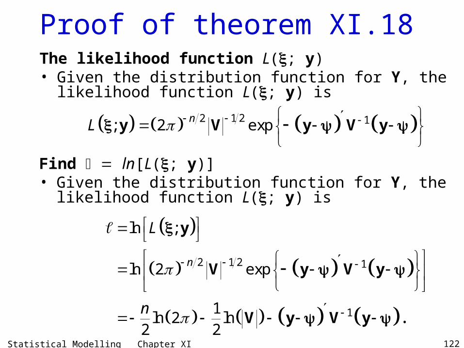
Statistical Modelling Chapter XI 122
Proof of theorem XI.18The likelihood function L(; y)• Given the distribution function for Y, the likelihood
function L(; y) is
1 22 1; 2 expnL y V y V y
Find ln[L(; y)]• Given the distribution function for Y, the likelihood
function L(; y) is
1 22 1
1
ln ;
ln 2 exp
1ln 2 ln
2 2.
n
L
n
y
V y V y
V y V y
Statistical Modelling Chapter XI 123
Proof of theorem XI.18 (continued)Maximize with respect to • The maximum likelihood estimates of are then obtained
by maximizing with respect to , that is, by differentiating with respect to and setting the result equal to zero.
• Clearly, the maximum likelihood estimates will be the solution of
• Now,
1 1
y V y y X V y X
0
1
1 1 12
y X V y X
y V y X V y X V X
Statistical Modelling Chapter XI 124
Proof of theorem XI.18 (continued)• and applying the rules for differentiation given in the proof
of theorem XI.1, we obtain
• Setting this derivative to zero we obtain
1 1 1
1 1 1
1 1
2
2
2 2
y V y X V y X V X
X V y X V X X V X
X V y X V X
1 1 1 12 2 0 or X V y X V X X V X X V y
Obtain the maximum likelihood estimators• Hence, as claimed. 1 1 X V X X V Y
So for general linear models the maximum likelihood and generalized least squares estimators coincide.
Statistical Modelling Chapter XI 125
XI.E Estimating the variance
a)Estimating the variance for the simple linear model
• As stated in theorem XI.11, and so to determine the variance of our OLS estimates need to know 2.
2var θ X X
• Generally, it is unknown and has to be estimated.• Now the definition of the variance is
var[Y] = E[(Y – E[Y])2].• The logical estimator is one that parallels this definition:
– put in our estimate for E[Y] and – replace the first expectation operator by the mean.
Statistical Modelling Chapter XI 126
Fitted values and residuals
• Definition XI.15: The fitted values are:– the estimated expected values for each
observation, . – obtained by substituting the x-values for each
observation into the estimated equation. – given by .
iE Y
ˆXθ
• The residuals are:– the deviations of the observed values of the
response variable from the fitted values. – denoted by – the estimates of .
ˆ e y Xθ Y Xθε
Statistical Modelling Chapter XI 127
Estimator of 2
• The logical estimator of 2 is: 2
ˆ ˆ ˆ ˆˆn n n
Y Xθ Y Xθ ε ε
• and our estimate would be ee/n.• Notice that the numerator of this expression measures
the spread of observed Y-values from the fitted equation. • We expect this to be random variation.• Turns out that this is the ML estimator as claimed in the
next theorem.
• Theorem XI.19: Let Y be a normally distributed random vector representing a random sample with E[Y] X and var[Y] VY 2In where X is an n q matrix of rank m q with n ≥ q, and is a q 1 vector of unknown parameters.
• The maximum likelihood estimator of 2 is denoted by and is given by
2
2n n n
Y Xθ Y Xθ ε ε
Proof: left as an exercise
Statistical Modelling Chapter XI 128
Is the estimator unbiased?• Theorem XI.20: Let • with
– Y the n 1 random vector of sample random variables, – X is an n q matrix of rank m q with n ≥ q, – is a q 1 vector of estimators of .
2 ˆ ˆˆn n Y Xθ Y Xθ
θ
• Then • so an unbiased estimator of 2 is
2 2ˆnn q
En
2ˆ ˆ
ˆn q n q
Y Xθ Y Xθ
• Proof: The proof of this theorem is postponed. • Latter estimator indicates how we might go more
generally, – once it is realized that this estimator is one that would
be obtained using the Residual MSQ from an ANOVA based on simple linear models.
Statistical Modelling Chapter XI 129
b) Estimating the variance for the general linear model
• Generally, the variance components (2s) that are the parameters of the variance matrix, V, can be estimated using the ANOVA method.
• Definition XI.16: The ANOVA method for estimating the variance components consists of equating the expected mean squares to the observed values of the mean squares and solving for the variance components.
Statistical Modelling Chapter XI 130
Example IV.1 Penicillin yield • This example involves 4 treatments applied using an
RCBD employing 5 Blends as blocks. • Suppose it was decided that the Blends are random. • The ANOVA table, with E[MSq]s, for this case is
Source df MSq E[MSq] F Prob Blends 4 66.0 2 2
BF B4 3.50 0.041
Flasks [Blends] 15
Treatments 3 23.3 2BF Tq 1.24 0.339
Residual 12 18.8 2BF
• The estimates of and are obtained as follows: 2
BF 2B
2 2BF B
2BF
4 66.0
18.8
22 BFB
66.0 ˆˆ
466.0 18.8
411.8.
so that 2BF 18.8
• That is, the magnitude of the two components of variation is similar.
Statistical Modelling Chapter XI 131
Example IV.1 Penicillin yield
2 2BF Bvar 18.8 11.8 30.6ˆ ˆijkY • so that
(see variance matrix in section XI.A, Linear models for designed experiments, above),
2 2BF Bvar ijkY
• Now
• Clearly, the two components make similar contributions to the variance of an observation.
Statistical Modelling Chapter XI 132
XI.G Exercises• Ex. 11-1 asks you to provide matrix expressions for
models and the estimator of the expected values.• Ex. 11-2 involves a generalized inverse and its use.• Ex. 11-3 asks you to derive the variance of the estimator
of the expected values.• Ex. 11-4 involves identifying estimable parameters and
the estimator of expected values for a factorial experiment.
• Ex. 11-5 asks for the E[Msq], matrix expressions for V and estimates of variance components.