36
XIV. Economic development and policies in 1960s, end of Bretton-Woods
| Date post: | 28-Dec-2015 |
| Category: |
Documents |
| Upload: | melissa-chandler |
| View: | 214 times |
| Download: | 0 times |

XIV. Economic development and policies in 1960s, end of
Bretton-Woods

XIV.1 Keynesian framework
General principles
Keynesian belief in demand side management• Insufficient demand – expansionary policy– Fiscal: higher governmental
expenditures, lower taxes–Monetary: increase of nominal money,
support for the decrease on interest rates (lower the official discount, obligatory reserves of the banking sector, open market operations)
• Demand too high - restrictions
Building blocks: Okun’s law (1)
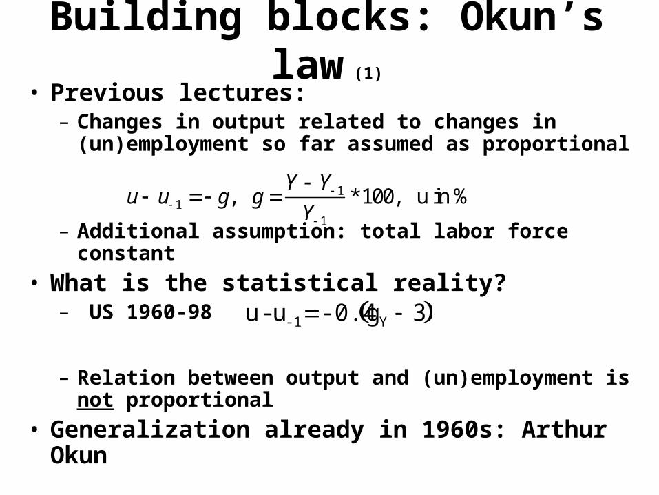
• Previous lectures:– Changes in output related to changes in
(un)employment so far assumed as proportional
– Additional assumption: total labor force constant
• What is the statistical reality?– US 1960-98
– Relation between output and (un)employment is not proportional
• Generalization already in 1960s: Arthur Okun
u - u-1 -0.4 gY 3
u u 1 g, g Y Y 1
Y 1
*100, u in %
Building blocks: Okun’s law (2)
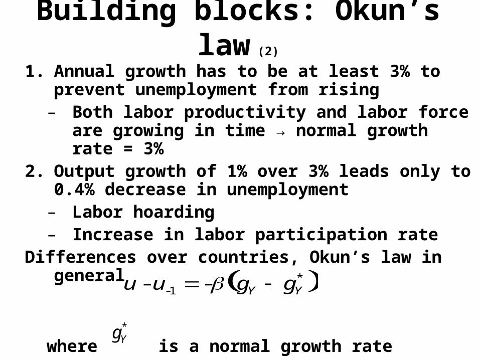
1. Annual growth has to be at least 3% to prevent unemployment from rising– Both labor productivity and labor force are
growing in time → normal growth rate = 3%2. Output growth of 1% over 3% leads only to
0.4% decrease in unemployment– Labor hoarding– Increase in labor participation rate
Differences over countries, Okun’s law in general
where is a normal growth rate
u - u-1 - gY gY*
gY*
Building block: Phillips curve
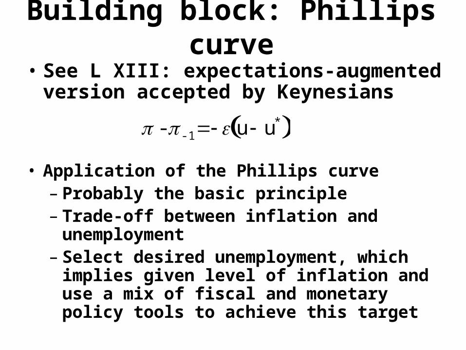
• See L XIII: expectations-augmented version accepted by Keynesians
• Application of the Phillips curve– Probably the basic principle– Trade-off between inflation and
unemployment– Select desired unemployment, which
implies given level of inflation and use a mix of fiscal and monetary policy tools to achieve this target
- -1 u u*
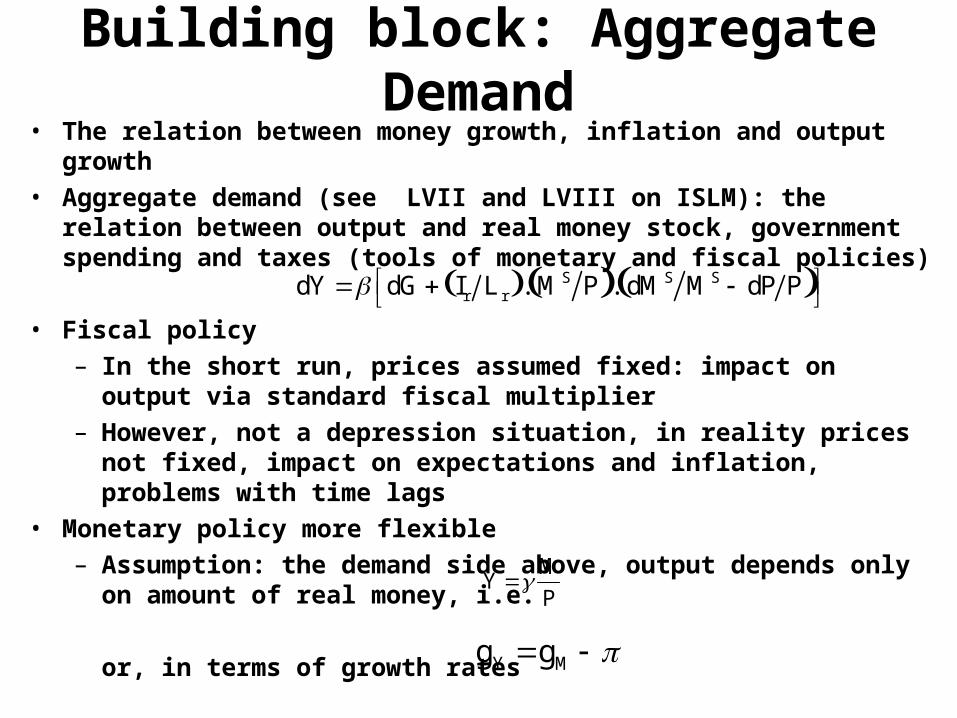
Building block: Aggregate Demand• The relation between money growth, inflation and output growth• Aggregate demand (see LVII and LVIII on ISLM): the relation
between output and real money stock, government spending and taxes (tools of monetary and fiscal policies)
• Fiscal policy– In the short run, prices assumed fixed: impact on output via
standard fiscal multiplier– However, not a depression situation, in reality prices not fixed,
impact on expectations and inflation, problems with time lags• Monetary policy more flexible
– Assumption: the demand side above, output depends only on amount of real money, i.e.
or, in terms of growth rates
dY dG Ir L r . MS P . dMS MS dP P
Y M
P
gY gM

Money growth, inflation and output growth
• Application of fiscal policies in 1960s - see bellow– However, too many obstacles
• Re-birth on monetary policies even in the Keynesian framework - medium term, economies converge to natural values, neoclassical synthesis
• Three basic equations above, for AD only relevant is money growth
• Exercise: try to see what happens if - e.g. - decrease of money growth
• Keynesian framework: smoothing the cycle, stop and go policies
u - u-1 - gY gY*
- -1 u u*
gY gM

StabilizationLong term: stabilization in the logic of
neoclassical synthesis• Economies converge towards long term
equilibriaExistence of inherent business cycles - need
for anti-cyclical policies• Discretionary policies, fine tuning• Built-in stabilizers• Budget deficit• Increase of the importance of the tax
policies

XIV.2 Monetarist framework

Implications of expectations-augmented Phillips curve
• Difference from Keynesian approach: there is no permanent trade-off between inflation and unemployment– In the short-run yes, but as soon as inflationary expectations
adjust, the trade-off disappears → output and unemployment returns to natural levels
• Crucial: how the expectations are formed?• Both monetarists and neoclassical synthesis -
adaptive expectation hypothesis (AEH):
• or
Pe P 1 1 P 1e P 1 , 0 1
Pe P Pe

Policy implications
• By repeating back substitution: expected inflation becomes a geometrically weighted average of past actual inflations– Larger weight given to the most recent
actual inflations
• Practical policy implication: there is a time gap between an increase in actual inflation and an increase in natural rate → allows for a temporary reduction of unemployment bellow

The accelerationist hypothesis• The fallacy of Keynesian approach: any
attempt to maintain unemployment permanently bellow the natural rate → acceleration of inflation → need for permanent increase of money growth– People will (sooner or later) adjust the expectations
→ to maintain unemployment under natural level → need for even higher inflation, etc.
– On labor market: need for permanent real wage bellow an equilibrium level → permanent increase of wages, prices, etc.
• End result: permanent accelerating inflation

The role of monetary policies• Vertical LRPC: aggregate demand management can
affect output and unemployment in the short-run only - is a discretionary monetary policy a viable option?– Yes, in case there is an urgent need to deal with strong external
disturbance and/or the time lag between increase in actual inflation and expectations adjustment is long
• Main monetarist policy proposition: fixed rate of monetary growth, consistent with long run growth potential of the economy. Main reasons:– Steady money growth → economy settles around natural
values and steady inflation– Capitalist economies are stable around natural values
(compare with Keynesianism above)!– Discretionary monetary policies may be destabilizing– As we don’t know exactly where the natural values are,
attempts to stabilize unemployment may lead to inflation ↔ inflation larger evil than unemployment

XIV.3 Policies under B-W system
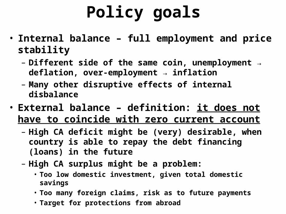
Policy goals
• Internal balance – full employment and price stability– Different side of the same coin, unemployment →
deflation, over-employment → inflation– Many other disruptive effects of internal disbalance
• External balance – definition: it does not have to coincide with zero current account– High CA deficit might be (very) desirable, when
country is able to repay the debt financing (loans) in the future
– High CA surplus might be a problem:• Too low domestic investment, given total domestic savings• Too many foreign claims, risk as to future payments• Target for protections from abroad

Policy options (1)
• Reminder from Ch.XII: at fix, monetary policy inefficient and domestic interest equals foreign one
• Maintaining internal balance – assume:– Economy at equilibrium with full employment
– Investment exogenous, taxes as well, short run: P and P* fixed
– Net export being a function of real ExR and disposable income:
– then equilibrium condition for a goods market
defines combinations of E and fiscal policy expansion (either G↑ or T↓) that maintain this equilibrium (output on potential level)
NX NX E.P* P,Yf - T
Yf C Yf - T I G NX E.P* P,Yf - T

Policy options (2)
• Maintaining the external balance:– suppose that there is a desirable level of CA deficit NXX– The equation
defines combinations of E and fiscal expansion that maintain desired deficit NXX
• Simultaneous achievement of external and internal balance – solution of 2 equations above, see next slide
• Four areas– I: over-employment and inflation, CA surplus too high– II: over-employment and inflation, CA deficit too high– III: underemployment and deflation, CA deficit too high– IV: underemployment and deflation, CA surplus too high
NXX NX E.P* P,Yf - T

E
Fiscal expansion
Internal balance, Yf
External balance, NX=NXX
I
II
III
IV
E
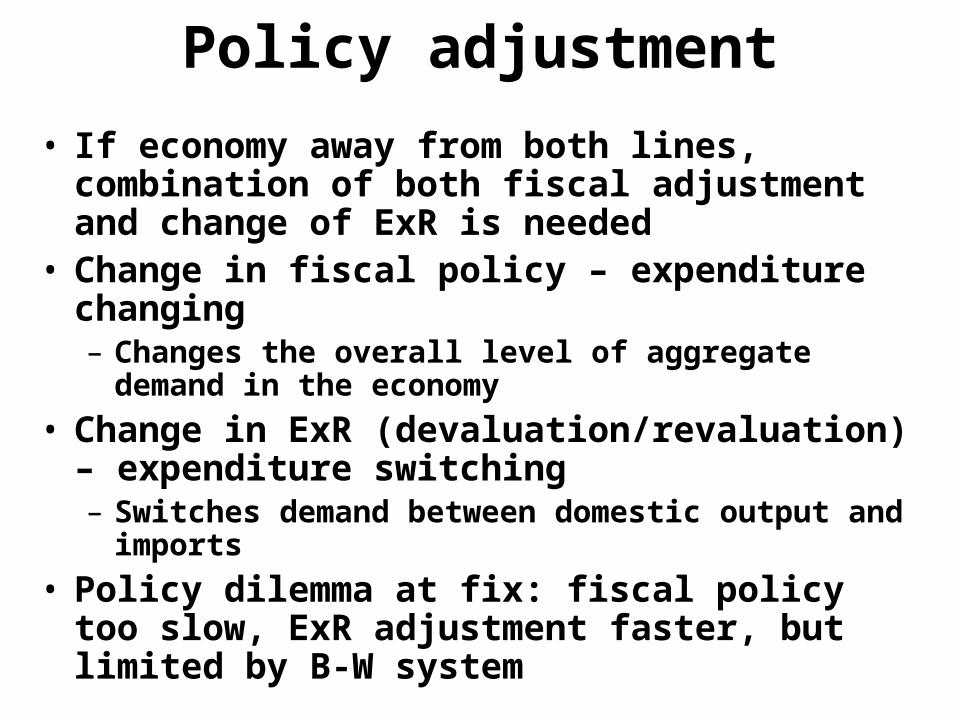
Policy adjustment
• If economy away from both lines, combination of both fiscal adjustment and change of ExR is needed
• Change in fiscal policy – expenditure changing– Changes the overall level of aggregate demand in
the economy
• Change in ExR (devaluation/revaluation) – expenditure switching– Switches demand between domestic output and
imports
• Policy dilemma at fix: fiscal policy too slow, ExR adjustment faster, but limited by B-W system
XIV.4 Economic reality and policies1955-1970
• In LIX: post-war reconstruction and policies up to (approximately) 1955– Introduction to Bretton-Woods system
• LXIV.1-3 above: both Keynesian and monetarist framework for economic policies
• This and subsequent sub-sections: economic reality of 1955-1970– Data– The success and failure of different policies
XIV.4.1 US Fiscal and Monetary Policy in the 1960s
• Closed economy
• US: till 1960s, BoP deficit did not limit the freedom of policies
• Logic: economic potential, determined by– Volume of labor force– Accumulated capital– Technology, productivity

Potential supply
• Full capacity output – there is always a certain level of unemployment– Phillips curve: hypothetical zero
unemployment means danger of high inflation
• Target full output: compromise between costs of unemployment vs. costs of inflation → potential output
Demand management in 1960s
• Given potential output
• Fiscal and monetary policies to stimulate or contain aggregate demand so that both unemployment and inflation kept of the “desired” levels and output close to the potential one

Fiscal policy
• Selection of tools: expenditures or taxes?– Expenditures: inflexible tool
• Time lags• Link to the budget deficits and debt
financing• Kennedy/Johnson tax cut 1963-4
– Growing economy, but less then potential output– Unemployment higher then target– Uneasy interpretation of results because of 1965
increase in expenditures due to the Vietnam War

Monetary policy
• Subdued to fiscal policy
• Even in 1960, basically “stop and go” nature–Monetary expansion in recession times:
1953-4, 1957-8, 1960-1– Restrictions under inflationary
pressures: 1952, 1955-7, after 1965, when inflation accelerated due to the military spending

XIV.4.2 Europe: The Golden Age
LIX: post-war reconstruction, strong fundamentals for subsequent economic growth
• Pro-market reforms• “Coordinated capitalism”– Direct governmental interventions (indicative
planning)– Social consensus on wage moderation,
profit retention and social securities
• Dawn of European integration– Positive effects from regional cooperation

Period of extensive growth• Persistent, very strong output growth– Wage restraint and high savings rates– Very high investment rates + FDI, namely from US– Common Market– Inflow of new labor force – “gastarbeiter”
immigration wave → very elastic labor supply
• Differences across the countries, but golden age for whole capitalist Europe– End of 1950s: incorporation of original laggards
(Belgium, Ireland, Denmark, Norway) and European periphery (Spain, Portugal, Greece)
• How long could have such an extensive growth lasted?

Problem: wage explosion and labor conflict
• Till beginning of 1960s: growth based on investment, investment based on wage restrain
• Since mid-1960s: new pressures, when “traditional” workers abandoned the social contracts and started to demand excessive wage increases– Social unrest in whole Europe 1968-1969
• Reasons:– Deep fall of unemployment, not wage disciplination any
more– People not ready to sacrifice for the sake of
reconstruction and growth any more– Memories of Great Depression faded away – new
generation

Problem: inflationary expectation and failure of Keynesian policies• Mounting inflationary pressures: increase of
inflation and of inflationary expectations• Weakening of Bretton-Woods system →
devaluation expectations in too many countries → additional inflationary drive
• Keynesian policy of demand management– Contributed to increase of inflation– Believing in (short-run) Phillips curve and in
ability to keep unemployment below natural level: helped to increase the expectations
• Confirmation of monetarist worries and predictions

XIV.5 The End of Bretton-Woods System
1950s
• B-W system:– Countries limited in their monetary policies– Adjustment to disequilibria via international reserves
(gold, but mainly USD) → need for keeping reasonable level of reserves• To keep reserves → limits of convertibility and of capital flows
• Special position of US– USD as reserve currency, main task – keeping the USD
price of gold (35 USD per oz.)– Need to keep gold reserves enough– Potential constraint on US macroeconomic policy – when
economies grow, will there be enough US gold reserves?• Confidence problem

1960s
• Gradual achievement of convertibility• Increase of international capital flows (despite
controls), more and more of speculative nature, because of expected devaluations
• More frequent balance of payments crises, accompanied by losses of foreign exchange reserves
• Devaluations, indeed (Britain November 1967)• Need for policies to achieve both internal and
external balance• All this: crucially dependent on the performance
of the US economy

US economy in 1960s• Vietnam War, “moon racing” and Great
Society program of President Johnson → strong fiscal expansion → inflation → worsening of CA → monetary policy only temporary contracted, later eased → further inflation → expected rise in USD price of gold
• Private speculators started to buy gold → two-tier gold market (private, where price of gold allowed to float; official, where fixed) → end of automatic constraint on worldwide monetary growth
US recession in 1970• 1970: US recession with increase of unemployment,
output falling, CA deficit → need for real devaluation of USD vis-à-vis major other currencies– Fall US prices – no way because of recession– Second option – nominal devaluation of USD, uneasy, as all
other countries should be willing to peg their currency to USD at new (devalued) rate
– August 15, 1971 – President Nixon stopped automatic exchange of gold for dollars and introduced import surcharge
• Multilateral negotiation → Smithonian agreement in December 1971– USD devalued by 10 % against foreign currencies, price of
gold increased to 38 USD per oz.• Not the end of the story yet: because of continuing
disequilibria, another speculative attack on USD in February 1973 → European currencies abandoned fix and by March 19, 1973 Japan and Europe floated their currencies against USD → end of B-W system

Literature to Ch. XIVOn Keynesian policies:• Blanchard, Macroeconomics, Ch. IXOn monetarist policies:• Snowdon, Vane, Modern Macroeconomic, Ch.4 (and literature there)On Bretton-Woods:• Krugman, Obstfeld, Chapter 18• Solomon, R., The International Monetary System 1945-1976. Harper&Row
1977• Bordo, Michael D., Eichengreen, B., A Retrospective on Bretton Woods
System, Chicago University Press, 1993US economy:• almost all medium level textbook of macroeconomics provide at least
some case studies from this period• Smith, W.L., Teigen, R.L. (1970), Readings in Money, National Income and
Stabilization Policy, Richard Irwin. Chapters 4 and 5 provide the best overview of the US economic policies in 1950s and 1960s. No need to read everything, but introductions to both chapters are good to know plus articles of Okun (p.313 and 345) and of Council of Economic Advisers.
European economy:• Eichengreen, B., The European Economy Since 1945. Princeton University
Press, 2007, Chapters 7-8


