165
Introduction to XPPAUT Mathieu Desroches [email protected] Session A3: Mathematics for oscillations 24-25 July
| Date post: | 13-Apr-2018 |
| Category: |
Documents |
| Upload: | mathbiology |
| View: | 252 times |
| Download: | 1 times |

7/27/2019 Xppaut Roscoff
http://slidepdf.com/reader/full/xppaut-roscoff 1/165
Introduction to XPPAUTMathieu [email protected]
Session A3: Mathematics for oscillations
24-25 July

7/27/2019 Xppaut Roscoff
http://slidepdf.com/reader/full/xppaut-roscoff 2/165
Introduction to XPPAUT
‘XPP-’ ‘-AUT’...

7/27/2019 Xppaut Roscoff
http://slidepdf.com/reader/full/xppaut-roscoff 3/165
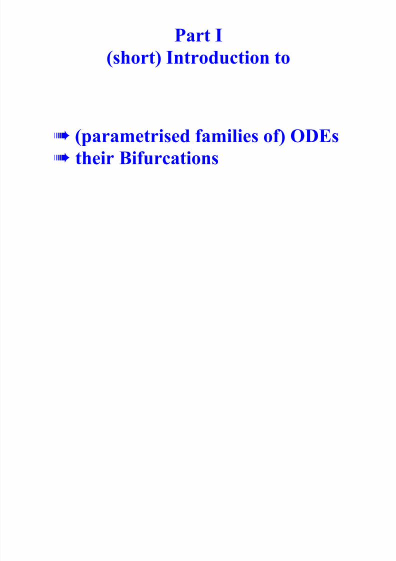
Part I
(short) Introduction to
! (parametrised families of) ODEs! their Bifurcations
! direct simulation of ODEs
! numerical continuation study

7/27/2019 Xppaut Roscoff
http://slidepdf.com/reader/full/xppaut-roscoff 4/165
Part I
(short) Introduction to
! (parametrised families of) ODEs! their Bifurcations
! direct simulation of ODEs
! numerical continuation study
7/27/2019 Xppaut Roscoff
http://slidepdf.com/reader/full/xppaut-roscoff 5/165
Part I
(short) Introduction to
! (parametrised families of) ODEs! their Bifurcations
! direct simulation of ODEs
! numerical continuation study

7/27/2019 Xppaut Roscoff
http://slidepdf.com/reader/full/xppaut-roscoff 6/165
Part I
(short) Introduction to
! (parametrised families of) ODEs! their Bifurcations
! direct simulation of ODEs
! numerical continuation study

7/27/2019 Xppaut Roscoff
http://slidepdf.com/reader/full/xppaut-roscoff 7/165
Part I
(short) Introduction to
! (parametrised families of) ODEs! their Bifurcations
! direct simulation of ODEs
! numerical continuation study

7/27/2019 Xppaut Roscoff
http://slidepdf.com/reader/full/xppaut-roscoff 8/165
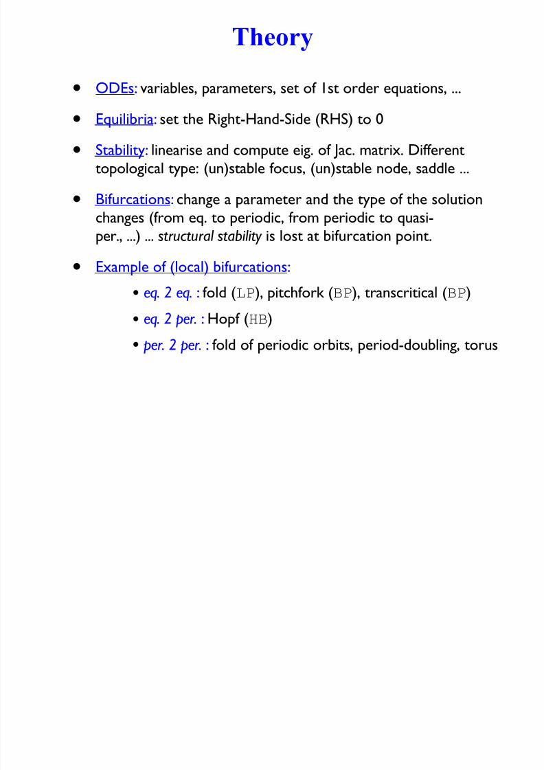
• ODEs: variables, parameters, set of 1st order equations, ...
• Equilibria: set the Right-Hand-Side (RHS) to 0
• Stability: linearise and compute eig. of Jac. matrix. Different
topological type: (un)stable focus, (un)stable node, saddle ...
• Bifurcations: change a parameter and the type of the solution
changes (from eq. to periodic, from periodic to quasi-
per., ...) ... structural stability is lost at bifurcation point.
• Example of (local) bifurcations:
Theory
• eq. 2 eq. : fold (LP), pitchfork (BP), transcritical (BP)
• eq. 2 per. : Hopf (HB)
• per. 2 per. : fold of periodic orbits, period-doubling, torus
7/27/2019 Xppaut Roscoff
http://slidepdf.com/reader/full/xppaut-roscoff 9/165
• ODEs: variables, parameters, set of 1st order equations, ...
• Equilibria: set the Right-Hand-Side (RHS) to 0
• Stability: linearise and compute eig. of Jac. matrix. Different
topological type: (un)stable focus, (un)stable node, saddle ...
• Bifurcations: change a parameter and the type of the solution
changes (from eq. to periodic, from periodic to quasi-
per., ...) ... structural stability is lost at bifurcation point.
• Example of (local) bifurcations:
Theory
• eq. 2 eq. : fold (LP), pitchfork (BP), transcritical (BP)
• eq. 2 per. : Hopf (HB)
• per. 2 per. : fold of periodic orbits, period-doubling, torus

7/27/2019 Xppaut Roscoff
http://slidepdf.com/reader/full/xppaut-roscoff 10/165
• ODEs: variables, parameters, set of 1st order equations, ...
• Equilibria: set the Right-Hand-Side (RHS) to 0
• Stability: linearise and compute eig. of Jac. matrix. Different
topological type: (un)stable focus, (un)stable node, saddle ...
• Bifurcations: change a parameter and the type of the solution
changes (from eq. to periodic, from periodic to quasi-
per., ...) ... structural stability is lost at bifurcation point.
• Example of (local) bifurcations:
Theory
• eq. 2 eq. : fold (LP), pitchfork (BP), transcritical (BP)
• eq. 2 per. : Hopf (HB)
• per. 2 per. : fold of periodic orbits, period-doubling, torus

7/27/2019 Xppaut Roscoff
http://slidepdf.com/reader/full/xppaut-roscoff 11/165
• ODEs: variables, parameters, set of 1st order equations, ...
• Equilibria: set the Right-Hand-Side (RHS) to 0
• Stability: linearise and compute eig. of Jac. matrix. Different
topological type: (un)stable focus, (un)stable node, saddle ...
• Bifurcations: change a parameter and the type of the solution
changes (from eq. to periodic, from periodic to quasi-
per., ...) ... structural stability is lost at bifurcation point.
• Example of (local) bifurcations:
Theory
• eq. 2 eq. : fold (LP), pitchfork (BP), transcritical (BP)
• eq. 2 per. : Hopf (HB)
• per. 2 per. : fold of periodic orbits, period-doubling, torus
7/27/2019 Xppaut Roscoff
http://slidepdf.com/reader/full/xppaut-roscoff 12/165
• ODEs: variables, parameters, set of 1st order equations, ...
• Equilibria: set the Right-Hand-Side (RHS) to 0
• Stability: linearise and compute eig. of Jac. matrix. Different
topological type: (un)stable focus, (un)stable node, saddle ...
• Bifurcations: change a parameter and the type of the solution
changes (from eq. to periodic, from periodic to quasi-
per., ...) ... structural stability is lost at bifurcation point.
• Example of (local) bifurcations:
Theory
• eq. 2 eq. : fold (LP), pitchfork (BP), transcritical (BP)
• eq. 2 per. : Hopf (HB)
• per. 2 per. : fold of periodic orbits, period-doubling, torus

7/27/2019 Xppaut Roscoff
http://slidepdf.com/reader/full/xppaut-roscoff 13/165
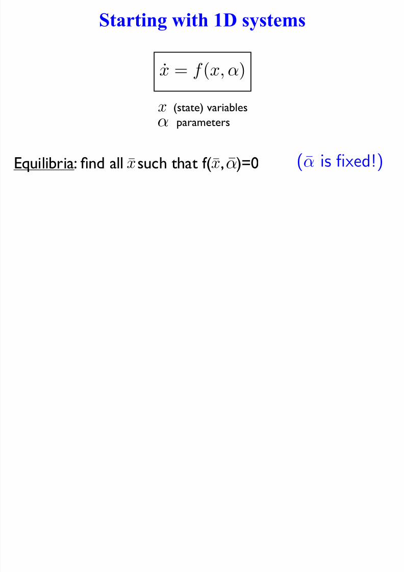
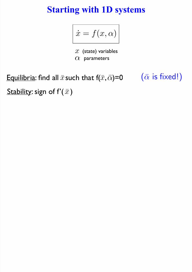
Starting with 1D systems
x (state) variables
parameters
x = f (x,α)
α
7/27/2019 Xppaut Roscoff
http://slidepdf.com/reader/full/xppaut-roscoff 14/165
Starting with 1D systems
x (state) variables
parameters
x = f (x,α)
αEquilibria: find all such that f( , )=0x x (α is fixed!)
α
7/27/2019 Xppaut Roscoff
http://slidepdf.com/reader/full/xppaut-roscoff 15/165
Starting with 1D systems
x (state) variables
parameters
Stability: sign of f ’( )x
x = f (x,α)
αEquilibria: find all such that f( , )=0x x (α is fixed!)
α

7/27/2019 Xppaut Roscoff
http://slidepdf.com/reader/full/xppaut-roscoff 16/165
Starting with 1D systems
x (state) variables
parameters
Stability: sign of f ’( )x
f’( )<0: is stable
f’( )>0: is unstable
x x
x x
x = f (x,α)
αEquilibria: find all such that f( , )=0x x (α is fixed!)
α

7/27/2019 Xppaut Roscoff
http://slidepdf.com/reader/full/xppaut-roscoff 17/165
1D systems ... let’s vary !

7/27/2019 Xppaut Roscoff
http://slidepdf.com/reader/full/xppaut-roscoff 18/165
1D systems ... let’s vary !
•Nothing changes in terms of ‘behaviour’:
! structural stability

7/27/2019 Xppaut Roscoff
http://slidepdf.com/reader/full/xppaut-roscoff 19/165
1D systems ... let’s vary !
•Nothing changes in terms of ‘behaviour’:
! structural stability
• Sudden change of stability when one varies !:
! bifurcation

7/27/2019 Xppaut Roscoff
http://slidepdf.com/reader/full/xppaut-roscoff 20/165

7/27/2019 Xppaut Roscoff
http://slidepdf.com/reader/full/xppaut-roscoff 21/165
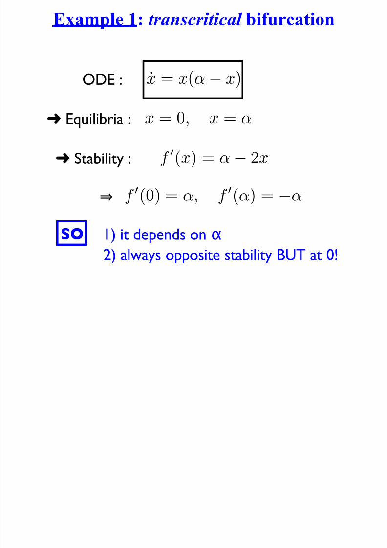
Example 1: transcritical bifurcation
" Equilibria : x = 0, x = α
x = x(α− x)ODE :

7/27/2019 Xppaut Roscoff
http://slidepdf.com/reader/full/xppaut-roscoff 22/165
Example 1: transcritical bifurcation
" Equilibria : x = 0, x = α
" Stability : f 0(x) = α− 2x
x = x(α− x)ODE :

7/27/2019 Xppaut Roscoff
http://slidepdf.com/reader/full/xppaut-roscoff 23/165
Example 1: transcritical bifurcation
" Equilibria : x = 0, x = α
" Stability : f 0(x) = α− 2x
f
0
(0) = α
, f
0
(α
) =−α
x = x(α− x)ODE :

7/27/2019 Xppaut Roscoff
http://slidepdf.com/reader/full/xppaut-roscoff 24/165
Example 1: transcritical bifurcation
" Equilibria : x = 0, x = α
" Stability : f 0(x) = α− 2x
f
0
(0) = α
, f
0
(α
) =−α
SO 1) it depends on !
x = x(α− x)ODE :
7/27/2019 Xppaut Roscoff
http://slidepdf.com/reader/full/xppaut-roscoff 25/165
Example 1: transcritical bifurcation
" Equilibria : x = 0, x = α
" Stability : f 0(x) = α− 2x
f
0
(0) = α
, f
0
(α
) =−α
SO 1) it depends on !
2) always opposite stability BUT at 0!
x = x(α− x)ODE :

7/27/2019 Xppaut Roscoff
http://slidepdf.com/reader/full/xppaut-roscoff 26/165
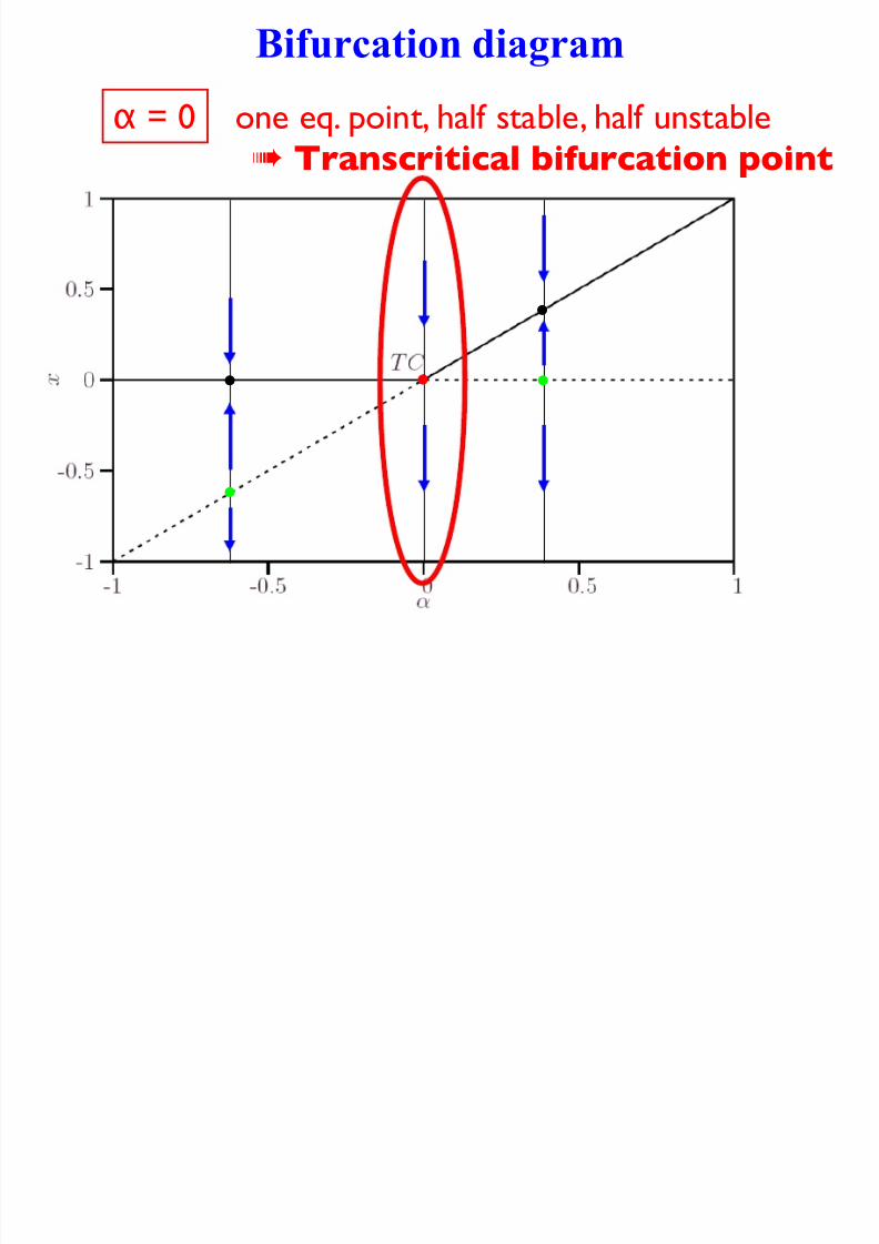
Bifurcation diagram
•
•
•
•
•

7/27/2019 Xppaut Roscoff
http://slidepdf.com/reader/full/xppaut-roscoff 27/165

7/27/2019 Xppaut Roscoff
http://slidepdf.com/reader/full/xppaut-roscoff 28/165
Bifurcation diagram
•
•
•
•
•
! = 0.4 > 0 x=! is stable & x=0 is unstable

7/27/2019 Xppaut Roscoff
http://slidepdf.com/reader/full/xppaut-roscoff 29/165
Bifurcation diagram
•
•
•
•
•
! = 0 one eq. point, half stable, half unstable
7/27/2019 Xppaut Roscoff
http://slidepdf.com/reader/full/xppaut-roscoff 30/165
Bifurcation diagram
•
•
•
•
•
! = 0 one eq. point, half stable, half unstable
! Transcritical bifurcation point

7/27/2019 Xppaut Roscoff
http://slidepdf.com/reader/full/xppaut-roscoff 31/165
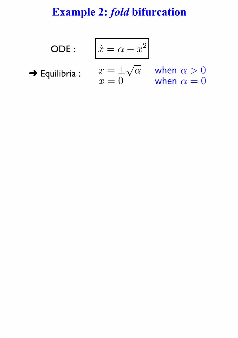
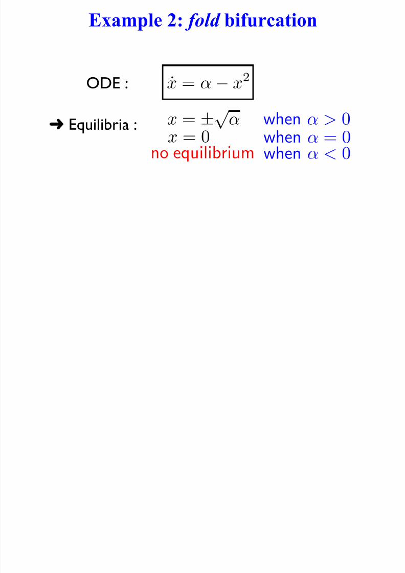
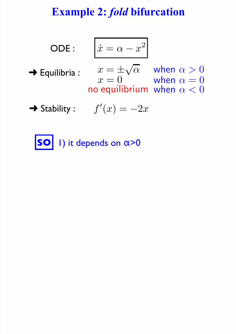
Example 2: fold bifurcation
ODE : x = α− x2

7/27/2019 Xppaut Roscoff
http://slidepdf.com/reader/full/xppaut-roscoff 32/165

7/27/2019 Xppaut Roscoff
http://slidepdf.com/reader/full/xppaut-roscoff 33/165
Example 2: fold bifurcation
ODE :
" Equilibria : x = ±√
α when α > 0
x = α− x2
7/27/2019 Xppaut Roscoff
http://slidepdf.com/reader/full/xppaut-roscoff 34/165
Example 2: fold bifurcation
ODE :
" Equilibria : x = ±√
α when α > 0
x = 0 when α
= 0
x = α− x2
7/27/2019 Xppaut Roscoff
http://slidepdf.com/reader/full/xppaut-roscoff 35/165
Example 2: fold bifurcation
ODE :
" Equilibria : x = ±√
α when α > 0
x = 0 when α = 0
when α < 0no equilibrium
x = α− x2

7/27/2019 Xppaut Roscoff
http://slidepdf.com/reader/full/xppaut-roscoff 36/165
7/27/2019 Xppaut Roscoff
http://slidepdf.com/reader/full/xppaut-roscoff 37/165
Example 2: fold bifurcation
ODE :
" Equilibria :
SO 1) it depends on !>0
x = ±√
α when α > 0
x = 0 when α = 0
when α < 0no equilibrium
x = α− x2
" Stability : f 0(x) = −2x
f ld if i

7/27/2019 Xppaut Roscoff
http://slidepdf.com/reader/full/xppaut-roscoff 38/165
Example 2: fold bifurcation
ODE :
" Equilibria :
SO 1) it depends on !>0
2) always opposite stability BUT at 0!
x = ±√
α when α > 0
x = 0 when α = 0
when α < 0no equilibrium
x = α−x2
" Stability : f 0(x) = −2x
Bif i di

7/27/2019 Xppaut Roscoff
http://slidepdf.com/reader/full/xppaut-roscoff 39/165
Bifurcation diagram
•
•
•
x = α− x2
Bif i di

7/27/2019 Xppaut Roscoff
http://slidepdf.com/reader/full/xppaut-roscoff 40/165
Bifurcation diagram
•
•
! = -0.5 < 0 no equilibrium point!
•
x = α− x2
Bif ti di

7/27/2019 Xppaut Roscoff
http://slidepdf.com/reader/full/xppaut-roscoff 41/165
Bifurcation diagram
•
•
! = 0.3 > 0 x=
"! is stable & x=-
"! is unstable
•
x = α− x2

7/27/2019 Xppaut Roscoff
http://slidepdf.com/reader/full/xppaut-roscoff 42/165

7/27/2019 Xppaut Roscoff
http://slidepdf.com/reader/full/xppaut-roscoff 43/165

7/27/2019 Xppaut Roscoff
http://slidepdf.com/reader/full/xppaut-roscoff 44/165

7/27/2019 Xppaut Roscoff
http://slidepdf.com/reader/full/xppaut-roscoff 45/165

7/27/2019 Xppaut Roscoff
http://slidepdf.com/reader/full/xppaut-roscoff 46/165
• IF there is an equilibrium point, it is either stable or unstable
• stable equilibrium: the system converges towards it as t#+#
• unstable equilibrium: the system converges towards it as t#-#
Summary: 1D systems ...

7/27/2019 Xppaut Roscoff
http://slidepdf.com/reader/full/xppaut-roscoff 47/165
• IF there is an equilibrium point, it is either stable or unstable
• stable equilibrium: the system converges towards it as t#+#
• unstable equilibrium: the system converges towards it as t#-#
Summary: 1D systems ...

7/27/2019 Xppaut Roscoff
http://slidepdf.com/reader/full/xppaut-roscoff 48/165
• IF there is an equilibrium point, it is either stable or unstable
• stable equilibrium: the system converges towards it as t#+#
• unstable equilibrium: the system converges towards it as t#-#
Summary: 1D systems ...
HoweverThe system is still nonlinear, so an exact
solution is unlikely to exist!
Same for equilibria!

7/27/2019 Xppaut Roscoff
http://slidepdf.com/reader/full/xppaut-roscoff 49/165
• IF there is an equilibrium point, it is either stable or unstable
• stable equilibrium: the system converges towards it as t#+#
• unstable equilibrium: the system converges towards it as t#-#
Summary: 1D systems ...
HoweverThe system is still nonlinear, so an exact
solution is unlikely to exist!
Same for equilibria!
$ Need to be able to simulate the system ...
N i l i l i f ODE

7/27/2019 Xppaut Roscoff
http://slidepdf.com/reader/full/xppaut-roscoff 50/165
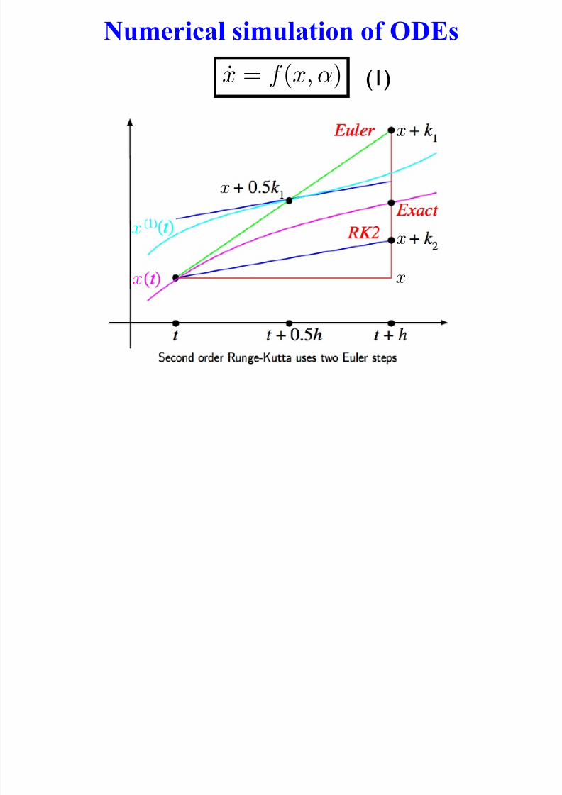
Numerical simulation of ODEs
x = f (x,α) (1)
N i l i l i f ODE

7/27/2019 Xppaut Roscoff
http://slidepdf.com/reader/full/xppaut-roscoff 51/165
Numerical simulation of ODEs
x = f (x,α) (1)
Idea $ discretise time :
$ ‘march’ in time :
Compute numerically approximate sol. to (1)?
x(t0) = x0 x(t1) = ...?
t0 t1 = t0 + h, h = “dt”
N i l i l ti f ODE

7/27/2019 Xppaut Roscoff
http://slidepdf.com/reader/full/xppaut-roscoff 52/165
Numerical simulation of ODEs
x = f (x,α) (1)
Idea $ discretise time :
$ ‘march’ in time :
Compute numerically approximate sol. to (1)?
x(t0) = x0 x(t1) = ...?
t0 t1 = t0 + h, h = “dt”
Example 1: Euler scheme
$ Error:
uses the slope of f(x(t0)) at x(t0)
to approximate x(t1)
(Taylor)
x(t1) ≈ x(t0) + f (x(t0),α)h
O(h2)
N i l i l ti f ODE

7/27/2019 Xppaut Roscoff
http://slidepdf.com/reader/full/xppaut-roscoff 53/165
Numerical simulation of ODEs
x = f (x,α) (1)
Example 1: Euler scheme
$ Error:
uses the slope of f(x(t0)) at x(t0)to approximate x(t1)
(Taylor)
x(t1) ≈ x(t0) + f (x(t0),α)h
O(h2)
Example 2: 2nd order Runge-Kutta scheme
$ Error: (Taylor)O(h3)
takes a half Euler step to the point (t0+0.5h, x(t0)+0.5k )
[see figure next]1
7/27/2019 Xppaut Roscoff
http://slidepdf.com/reader/full/xppaut-roscoff 54/165

7/27/2019 Xppaut Roscoff
http://slidepdf.com/reader/full/xppaut-roscoff 55/165
2D systems (nD n>2)
7/27/2019 Xppaut Roscoff
http://slidepdf.com/reader/full/xppaut-roscoff 56/165
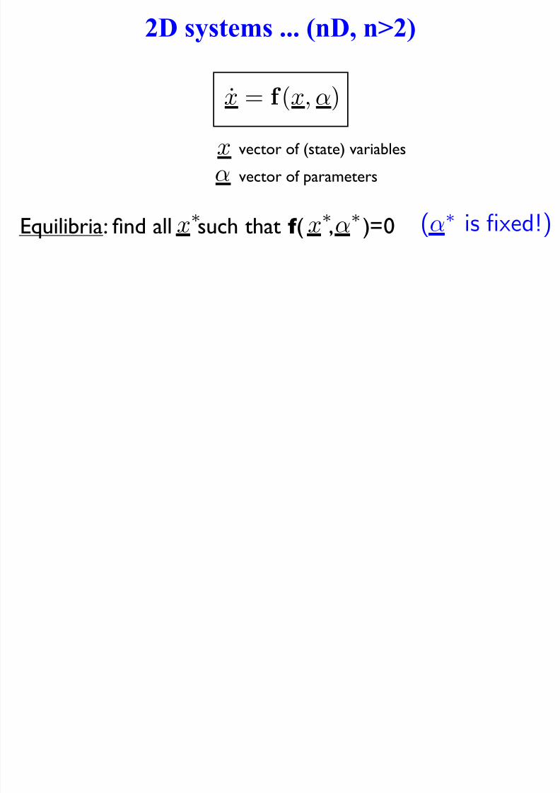
2D systems ... (nD, n>2)
vector of (state) variables
vector of parameters
x
α
x = f (x,α)
Equilibria: find all such that f ( , )=0x∗
α∗
x∗ (α∗ is fixed!)
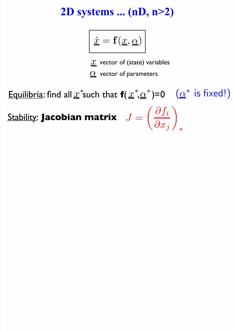
7/27/2019 Xppaut Roscoff
http://slidepdf.com/reader/full/xppaut-roscoff 57/165
2D systems (nD n>2)
7/27/2019 Xppaut Roscoff
http://slidepdf.com/reader/full/xppaut-roscoff 58/165
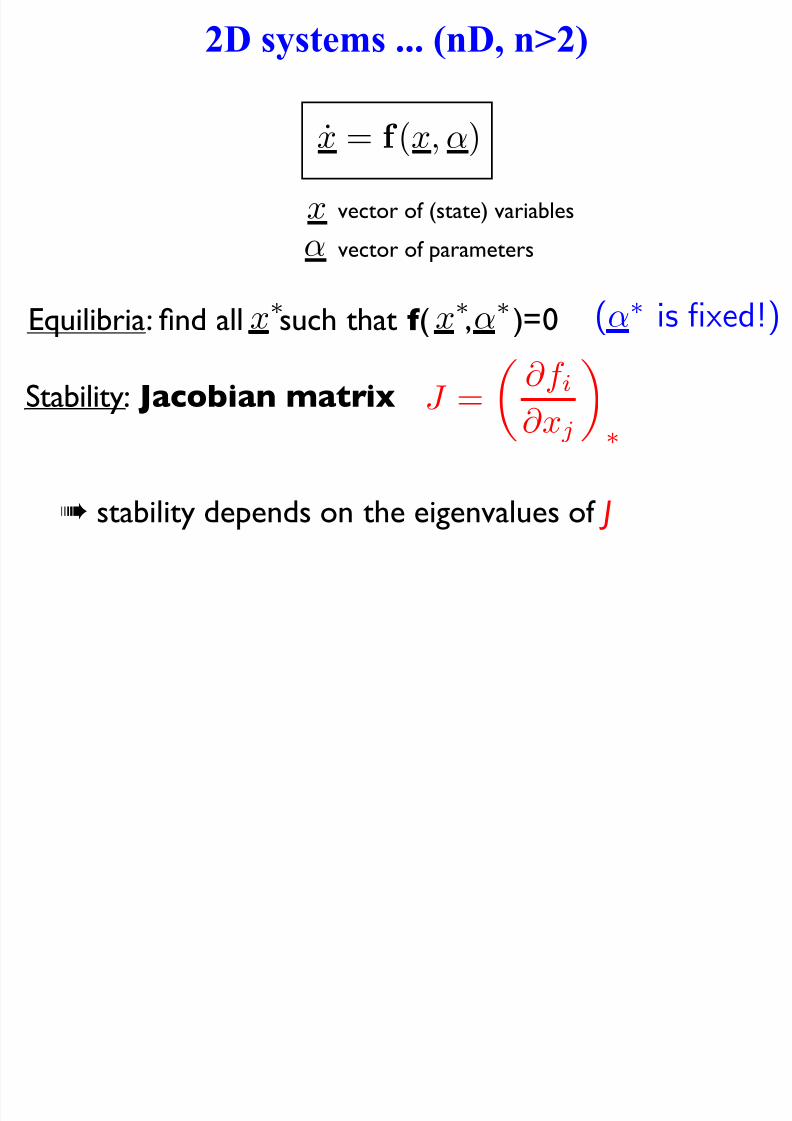
2D systems ... (nD, n>2)
vector of (state) variables
vector of parameters
x
α
x = f (x,α)
Stability: Jacobian matrix J = ∂ f i
∂ xj∗
! stability depends on the eigenvalues of J
Equilibria: find all such that f ( , )=0x∗
α∗
x∗ (α∗ is fixed!)
2D systems : nullclines

7/27/2019 Xppaut Roscoff
http://slidepdf.com/reader/full/xppaut-roscoff 59/165
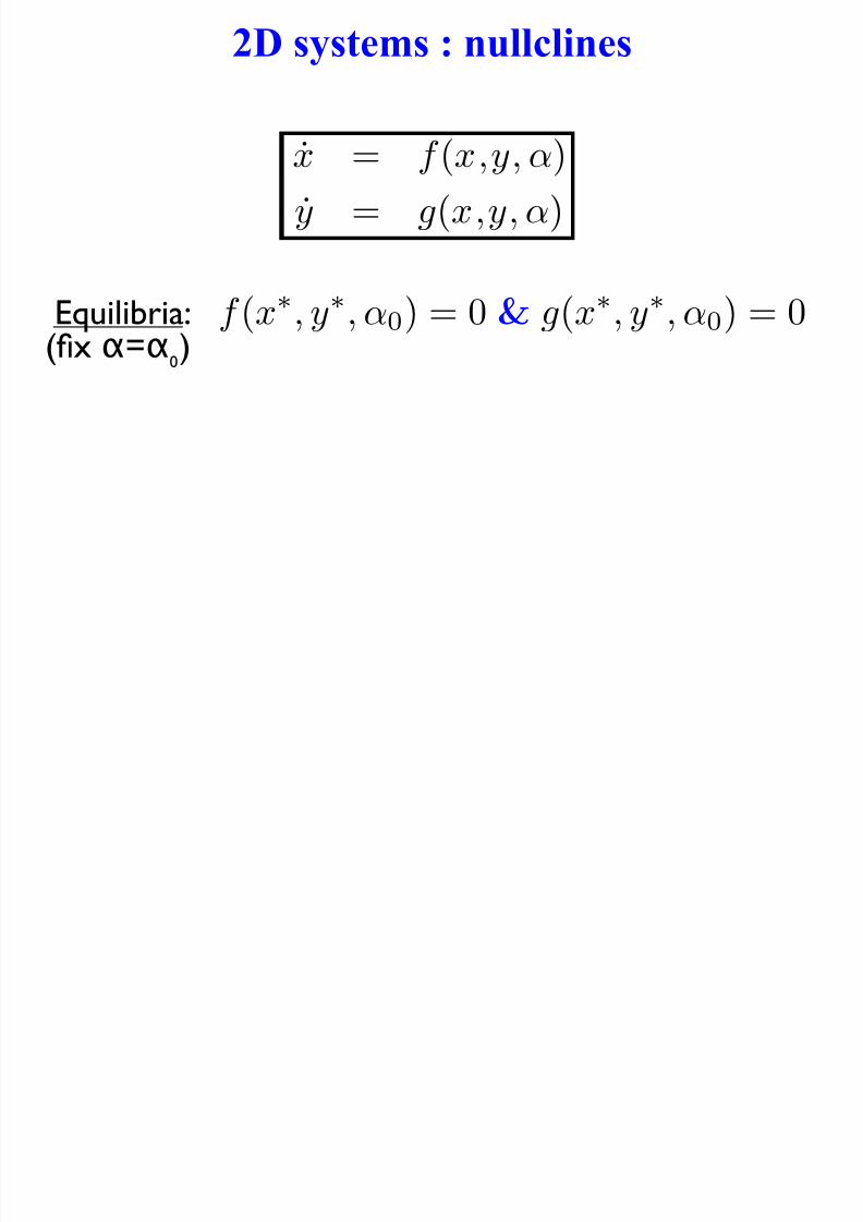
2D systems : nullclines
x = f (x,y,α)y = g(x,y,α)
2D systems : nullclines
7/27/2019 Xppaut Roscoff
http://slidepdf.com/reader/full/xppaut-roscoff 60/165
2D systems : nullclines
x = f (x,y,α)y = g(x,y,α)
Equilibria:(fix !=! )
0
f (x∗
, y∗
,α0) = 0 & g(x∗
, y∗
,α0) = 0
2D systems : nullclines
7/27/2019 Xppaut Roscoff
http://slidepdf.com/reader/full/xppaut-roscoff 61/165
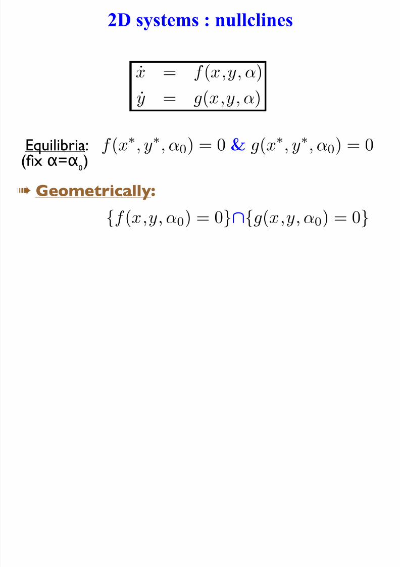
2D systems : nullclines
x = f (x,y,α)y = g(x,y,α)
Equilibria:(fix !=! )
0
f (x∗
, y∗
,α0) = 0 & g(x∗
, y∗
,α0) = 0
! Geometrically:
{f (x,y,α0) = 0}∩{g(x,y,α0) = 0}
7/27/2019 Xppaut Roscoff
http://slidepdf.com/reader/full/xppaut-roscoff 62/165
2D systems : nullclines

7/27/2019 Xppaut Roscoff
http://slidepdf.com/reader/full/xppaut-roscoff 63/165
y
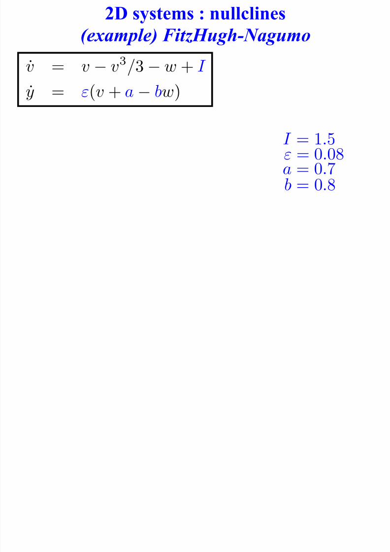
(example) FitzHugh-Nagumo
v = v−
v3
/3−
w + I y = ε(v + a − bw)
I = 1.5ε = 0.08
a = 0.7
b = 0.8
! f is cubic
! g is linear
2D systems : nullclines
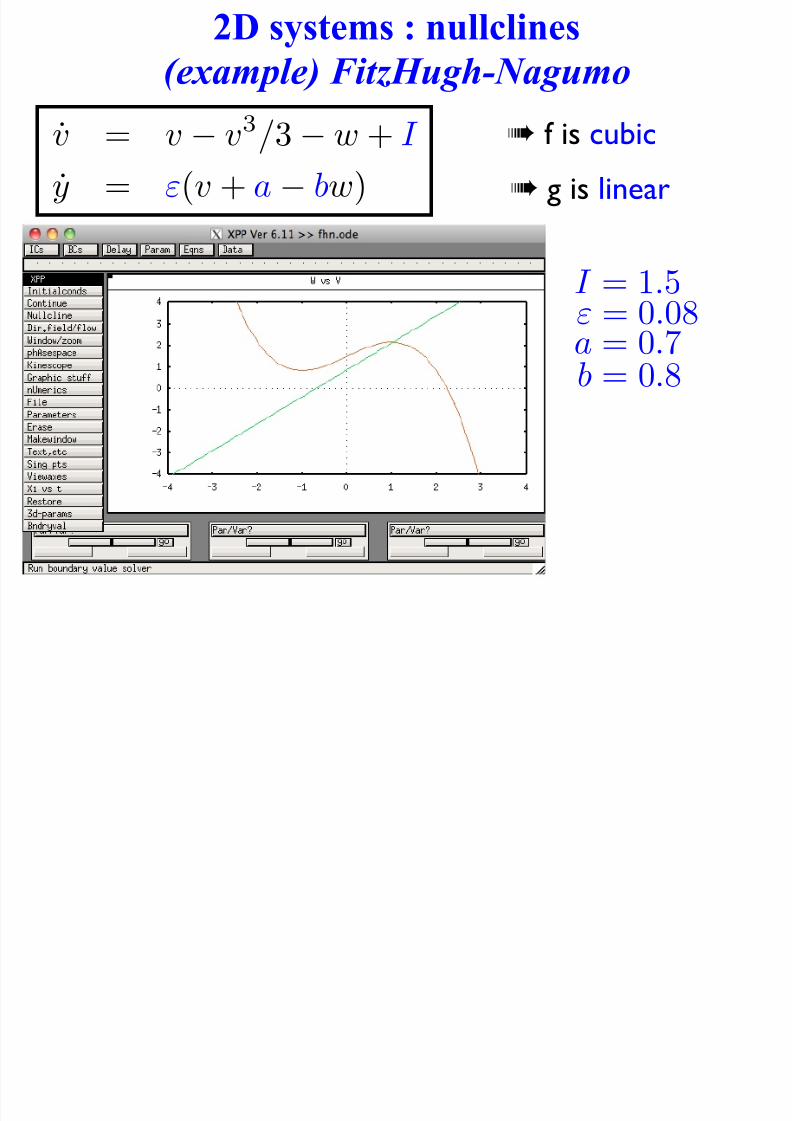
7/27/2019 Xppaut Roscoff
http://slidepdf.com/reader/full/xppaut-roscoff 64/165
y
(example) FitzHugh-Nagumo
v = v−
v3
/3−
w + I y = ε(v + a − bw)
I = 1.5ε = 0.08
a = 0.7
b = 0.8
! f is cubic
! g is linear
7/27/2019 Xppaut Roscoff
http://slidepdf.com/reader/full/xppaut-roscoff 65/165
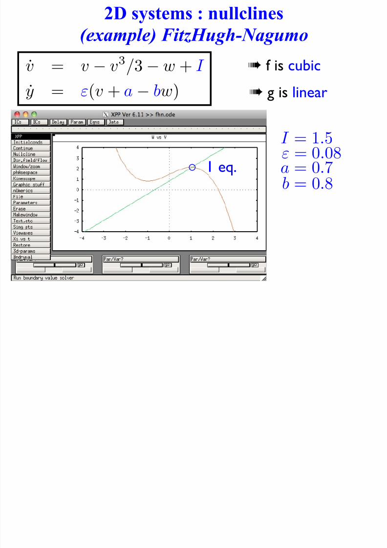
2D systems : nullclines
7/27/2019 Xppaut Roscoff
http://slidepdf.com/reader/full/xppaut-roscoff 66/165
y
(example) FitzHugh-Nagumo
v = v−
v3
/3−
w + I y = ε(v + a − bw)
ε = 0.08
a = 0.7
I = 0.4
b = 1.8
! f is cubic
! g is linear
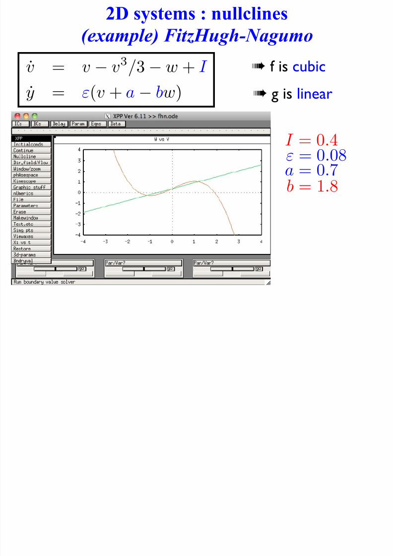
2D systems : nullclines

7/27/2019 Xppaut Roscoff
http://slidepdf.com/reader/full/xppaut-roscoff 67/165
y
(example) FitzHugh-Nagumo
v = v−
v3
/3−
w + I y = ε(v + a − bw)
ε = 0.08
a = 0.7
I = 0.4
b = 1.8◦◦
◦
3 eq.
! f is cubic
! g is linear
Linear a roximation: 2D case

7/27/2019 Xppaut Roscoff
http://slidepdf.com/reader/full/xppaut-roscoff 68/165
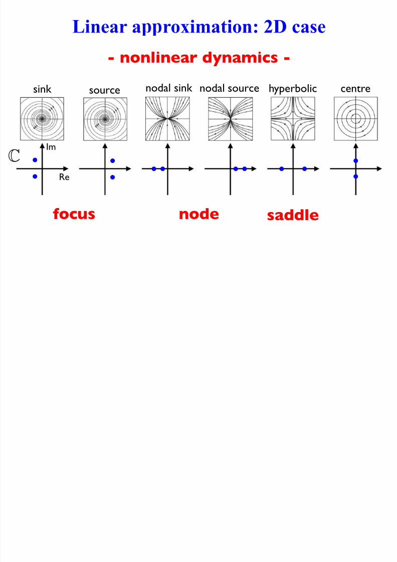
Linear a roximation: 2D case
sourcesink nodal sink nodal source hyperbolic centre
•
•
C •
•
•• •• ••
•
•Re
Im
Linear a roximation: 2D case

7/27/2019 Xppaut Roscoff
http://slidepdf.com/reader/full/xppaut-roscoff 69/165
Linear a roximation: 2D case
sourcesink nodal sink nodal source hyperbolic centre
•
•
C •
•
•• •• ••
•
•
- nonlinear dynamics -
Re
Im
Linear a roximation: 2D case

7/27/2019 Xppaut Roscoff
http://slidepdf.com/reader/full/xppaut-roscoff 70/165
Linear a roximation: 2D case
sourcesink nodal sink nodal source hyperbolic centre
•
•
C •
•
•• •• ••
•
•
focus
- nonlinear dynamics -
Re
Im
Linear a roximation: 2D case

7/27/2019 Xppaut Roscoff
http://slidepdf.com/reader/full/xppaut-roscoff 71/165
Linear a roximation: 2D case
sourcesink nodal sink nodal source hyperbolic centre
•
•
C •
•
•• •• ••
•
•
focus node
- nonlinear dynamics -
Re
Im
7/27/2019 Xppaut Roscoff
http://slidepdf.com/reader/full/xppaut-roscoff 72/165

7/27/2019 Xppaut Roscoff
http://slidepdf.com/reader/full/xppaut-roscoff 73/165
Linear a roximation: 2D case

7/27/2019 Xppaut Roscoff
http://slidepdf.com/reader/full/xppaut-roscoff 74/165
Linear a roximation: 2D case
sourcesink nodal sink nodal source hyperbolic centre
•
•
C •
•
•• •• ••
•
•
focus node saddle
- nonlinear dynamics -
(un)stable eigenspaces
! nonlinear equivalent: (un)stable manifolds
W s,u
Re
Im
7/27/2019 Xppaut Roscoff
http://slidepdf.com/reader/full/xppaut-roscoff 75/165
Bifurcations
7/27/2019 Xppaut Roscoff
http://slidepdf.com/reader/full/xppaut-roscoff 76/165
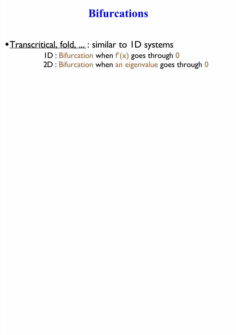
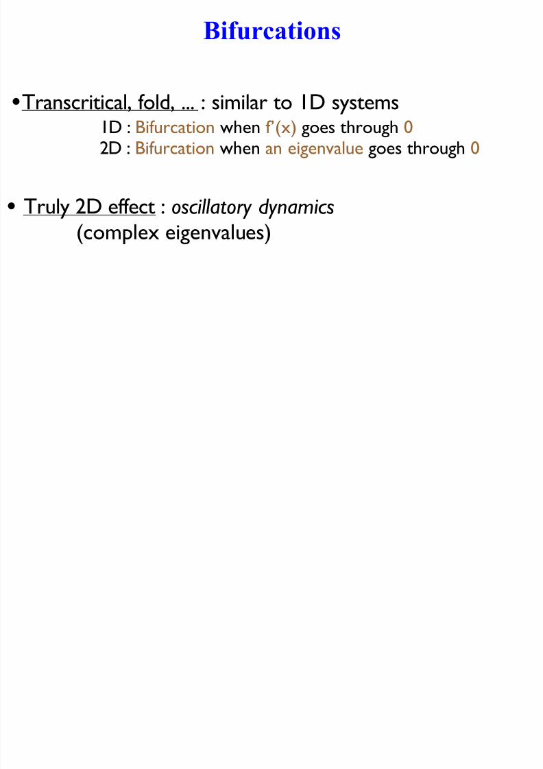
Bifurcations
•Transcritical, fold, ... : similar to 1D systems
Bifurcations
7/27/2019 Xppaut Roscoff
http://slidepdf.com/reader/full/xppaut-roscoff 77/165
Bifurcations
•Transcritical, fold, ... : similar to 1D systems1D : Bifurcation when f’(x) goes through 02D : Bifurcation when an eigenvalue goes through 0
Bifurcations
7/27/2019 Xppaut Roscoff
http://slidepdf.com/reader/full/xppaut-roscoff 78/165
Bifurcations
•Transcritical, fold, ... : similar to 1D systems
• Truly 2D effect : oscillatory dynamics
(complex eigenvalues)
1D : Bifurcation when f’(x) goes through 02D : Bifurcation when an eigenvalue goes through 0
Bifurcations

7/27/2019 Xppaut Roscoff
http://slidepdf.com/reader/full/xppaut-roscoff 79/165
Bifurcations
•Transcritical, fold, ... : similar to 1D systems
• Truly 2D effect : oscillatory dynamics
(complex eigenvalues)
1 - ‘Damped’ nonlin. oscillations: focus eq.
2 - ‘Sustained’ nonlin. oscillations: limit cycle
1D : Bifurcation when f’(x) goes through 02D : Bifurcation when an eigenvalue goes through 0

7/27/2019 Xppaut Roscoff
http://slidepdf.com/reader/full/xppaut-roscoff 80/165
Hopf bifurcation
7/27/2019 Xppaut Roscoff
http://slidepdf.com/reader/full/xppaut-roscoff 81/165
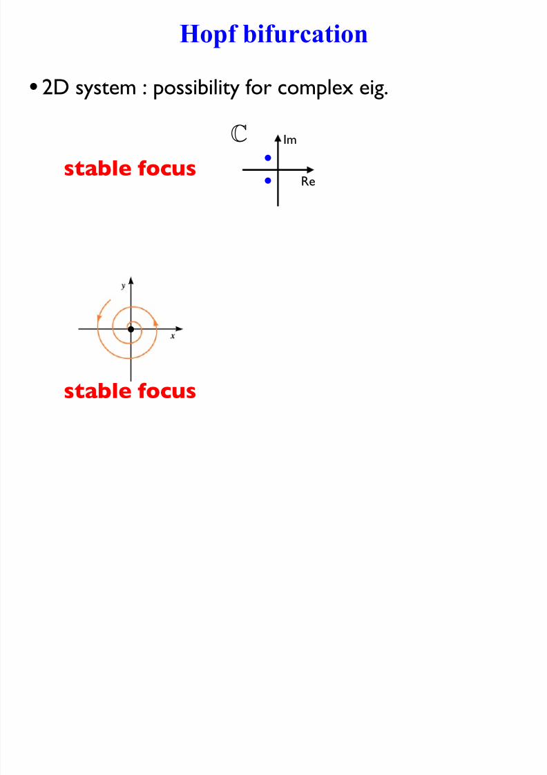
stable focus
Hopf bifurcation
• 2D system : possibility for complex eig.
•
•
C
Re
Im
stable focus
•
7/27/2019 Xppaut Roscoff
http://slidepdf.com/reader/full/xppaut-roscoff 82/165
Hopf bifurcation
7/27/2019 Xppaut Roscoff
http://slidepdf.com/reader/full/xppaut-roscoff 83/165
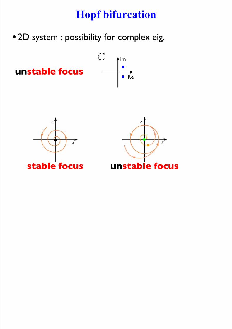
unstable focus
Hopf bifurcation
• 2D system : possibility for complex eig.
•
•
C
Re
Im
! focus eq. destabilises when eigenvalues cross Im
stable focus
• •
unstable focus
Hopf bifurcation

7/27/2019 Xppaut Roscoff
http://slidepdf.com/reader/full/xppaut-roscoff 84/165
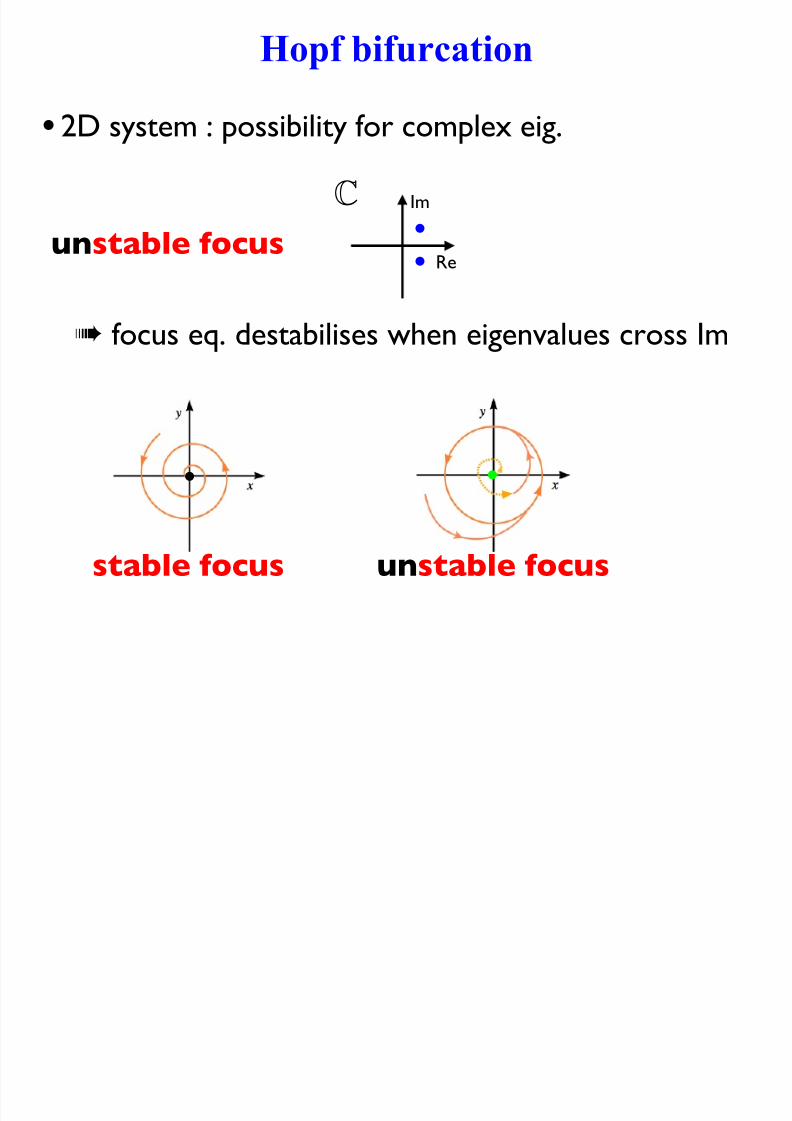
unstable focus
Hopf bifurcation
• 2D system : possibility for complex eig.
•
•
C
Re
Im
! focus eq. destabilises when eigenvalues cross Im
stable focus
• •
unstable focus
a stable
limit cycleis created!
Hopf : bifurcation diagram

7/27/2019 Xppaut Roscoff
http://slidepdf.com/reader/full/xppaut-roscoff 85/165
α
Measure of
the solution
αH
Hopf : bifurcation diagram

7/27/2019 Xppaut Roscoff
http://slidepdf.com/reader/full/xppaut-roscoff 86/165
α
Measure of
the solution
αH
Before : stable equilibrium
Hopf : bifurcation diagram
7/27/2019 Xppaut Roscoff
http://slidepdf.com/reader/full/xppaut-roscoff 87/165
α
Measure of
the solution
αH
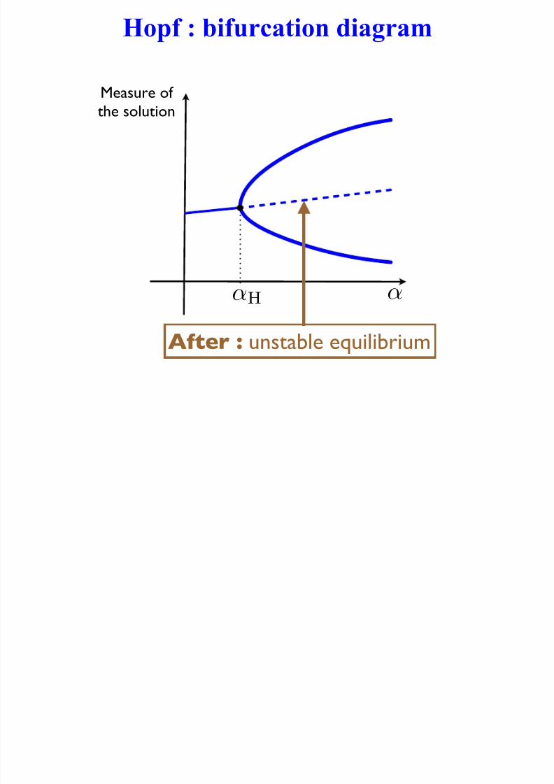
After : unstable equilibrium
Hopf : bifurcation diagram
7/27/2019 Xppaut Roscoff
http://slidepdf.com/reader/full/xppaut-roscoff 88/165
α
Measure of
the solution
αH
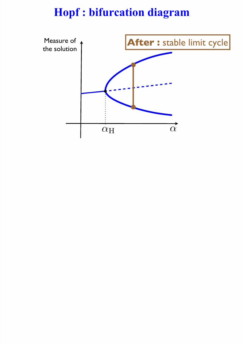
After : stable limit cycle
Hopf : bifurcation diagram
7/27/2019 Xppaut Roscoff
http://slidepdf.com/reader/full/xppaut-roscoff 89/165
α
Measure of
the solution
αH
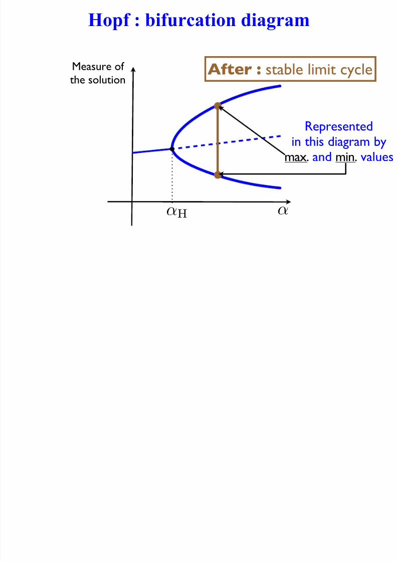
After : stable limit cycle
Represented
in this diagram bymax. and min. values
Hopf : bifurcation diagram

7/27/2019 Xppaut Roscoff
http://slidepdf.com/reader/full/xppaut-roscoff 90/165
α
Measure of
the solution
αH
After : stable limit cycle
Represented
in this diagram bymax. and min. values
From stationary to periodic when varying !!
Hopf : bifurcation diagram
3D i li i
7/27/2019 Xppaut Roscoff
http://slidepdf.com/reader/full/xppaut-roscoff 91/165
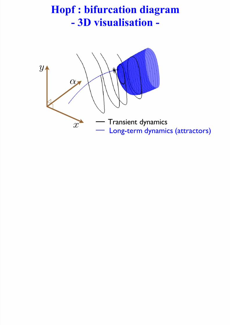
- 3D visualisation -
α
x
y
Transient dynamicsLong-term dynamics (attractors)
Numerical continuation : idea

7/27/2019 Xppaut Roscoff
http://slidepdf.com/reader/full/xppaut-roscoff 92/165
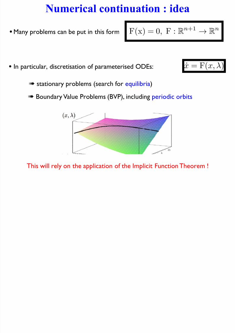
• Goal is to compute families (branches) of solutions of
nonlinear equations of the form:
F(x) = 0, F : Rn+1 → Rn
! under-determined system (one more unknowns than equations)
! away from singularities, solution set = 1-dim. manifold
embedded in (n+1)-dim. space
7/27/2019 Xppaut Roscoff
http://slidepdf.com/reader/full/xppaut-roscoff 93/165
Parameter continuation

7/27/2019 Xppaut Roscoff
http://slidepdf.com/reader/full/xppaut-roscoff 94/165
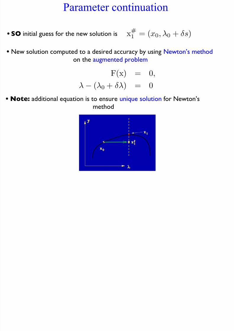
• Suppose we have one solution to the problem and wish to vary
one component to find a new solution ...
• In the I.F.T. holds at this point, then locally there is a branch
of solutions parameterised by $: (x($), $).
F(x0) = 0, x0 = (x0,λ0) ∈ Rn × R
• Small change in the parameter $ new point that is not a
solution of the problem but close to one!
x#
1 = (x0,λ0 + δ s),
F(x#1 ) 6= 0,
F(x#1 ) 1
Parameter continuation
7/27/2019 Xppaut Roscoff
http://slidepdf.com/reader/full/xppaut-roscoff 95/165
• SO initial guess for the new solution is
• New solution computed to a desired accuracy by using Newton’s method
on the augmented problem
• Note: additional equation is to ensure unique solution for Newton’s
method
x#1 = (x0,λ0 + δ s)
F(x) = 0,
λ−
(λ0 + δλ) = 0
7/27/2019 Xppaut Roscoff
http://slidepdf.com/reader/full/xppaut-roscoff 96/165
Problem at a fold !!

7/27/2019 Xppaut Roscoff
http://slidepdf.com/reader/full/xppaut-roscoff 97/165
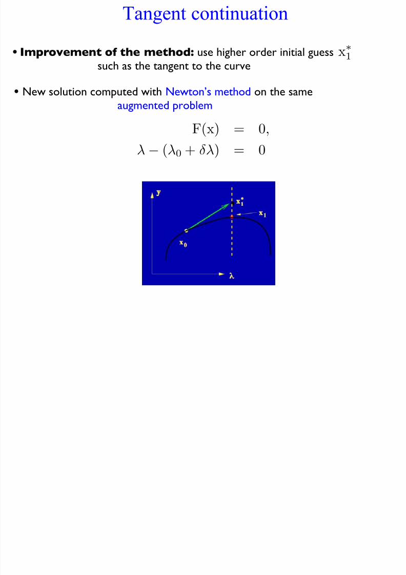
Keller’s pseudo-arclength continuation

7/27/2019 Xppaut Roscoff
http://slidepdf.com/reader/full/xppaut-roscoff 98/165
• Problem at a fold: the “parameter” chosen to do the
continuation cannot parameterise the solution curve
• Solution: parameterise by something that do not have this problem
!Arclength s along the curve !
• The problem to be solved becomes F(x) = 0,
(λ−
λ0)λ0 + (x−
x0)x0−
δ s = 0
Arclength measured along the tangent space !
Periodic orbit continuation

7/27/2019 Xppaut Roscoff
http://slidepdf.com/reader/full/xppaut-roscoff 99/165
• We look for periodic solutions of the problem :
! We seek for solutions of period 1 i.e. such that :
x = F(x(t),λ)
x0 = T F(x(t),λ)
x(1) = x(0)
! The true period T is now an additional parameter
• Note: the above equations do not uniquely specify x and T ...
... translation invariance !
! Necessity of a Phase condition
• Example: Poincaré orthogonality condition
• In practice: Integral phase condition
Z 1
0
xk(t)∗x0k−1
dt = 0
(xk(0)− xk−1(0))∗x0k−1(0)) = 0
• Fix the interval of periodicity by the transformation t # t/T
such that :
Periodic orbit continuation

7/27/2019 Xppaut Roscoff
http://slidepdf.com/reader/full/xppaut-roscoff 100/165
• We look for periodic solutions of the problem :
! We seek for solutions of period 1 i.e. such that :
x = F(x(t),λ)
x0 = T F(x(t),λ)
x(1) = x(0)
! The true period T is now an additional parameter
• Note: the above equations do not uniquely specify x and T ...
... translation invariance !
! Necessity of a Phase condition
• Example: Poincaré orthogonality condition
• In practice: Integral phase condition
Z 1
0
xk(t)∗x0k−1
dt = 0
(xk(0)− xk−1(0))∗x0k−1(0)) = 0
• Fix the interval of periodicity by the transformation t # t/T
such that :
Periodic orbit continuation

7/27/2019 Xppaut Roscoff
http://slidepdf.com/reader/full/xppaut-roscoff 101/165
• ... we then solve a large G(X) = 0 augmented by the
arclength-continuation equation:
• Discretisation of the periodic orbits: using orthogonalcollocation (piecewise polynomials on mesh intervals)
! Solve exactly at mesh points (boundaries of mesh intervals)
Z 1
0
(xk(t)− xk−1(t))∗xk−1dt + (T k − T k−1) T k−1
+(λk − λk−1)λk−1 − δ s = 0
! Inside mesh intervals: well-chosen collocation points (good
convergence properties)
• Well-posedness: n+1 unknowns (n components of x and period T)
for n+1 conditions ( periodicity + phase)
! varying 1 parameter will give a 1-parameter family of per. orbits

7/27/2019 Xppaut Roscoff
http://slidepdf.com/reader/full/xppaut-roscoff 102/165
Part II: XPPAUT
- main features & capabilities -
Equation file: FitzHugh-Nagumo
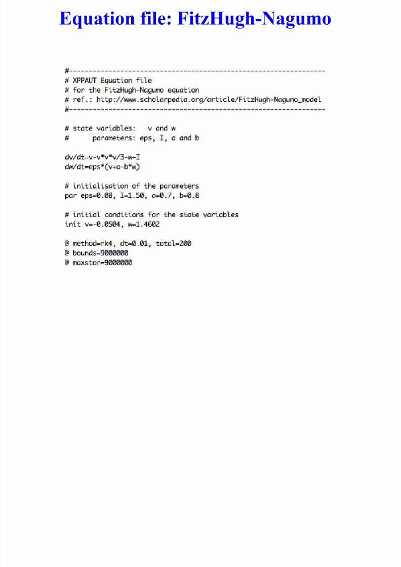
7/27/2019 Xppaut Roscoff
http://slidepdf.com/reader/full/xppaut-roscoff 103/165
Equation file: FitzHugh-Nagumo
7/27/2019 Xppaut Roscoff
http://slidepdf.com/reader/full/xppaut-roscoff 104/165
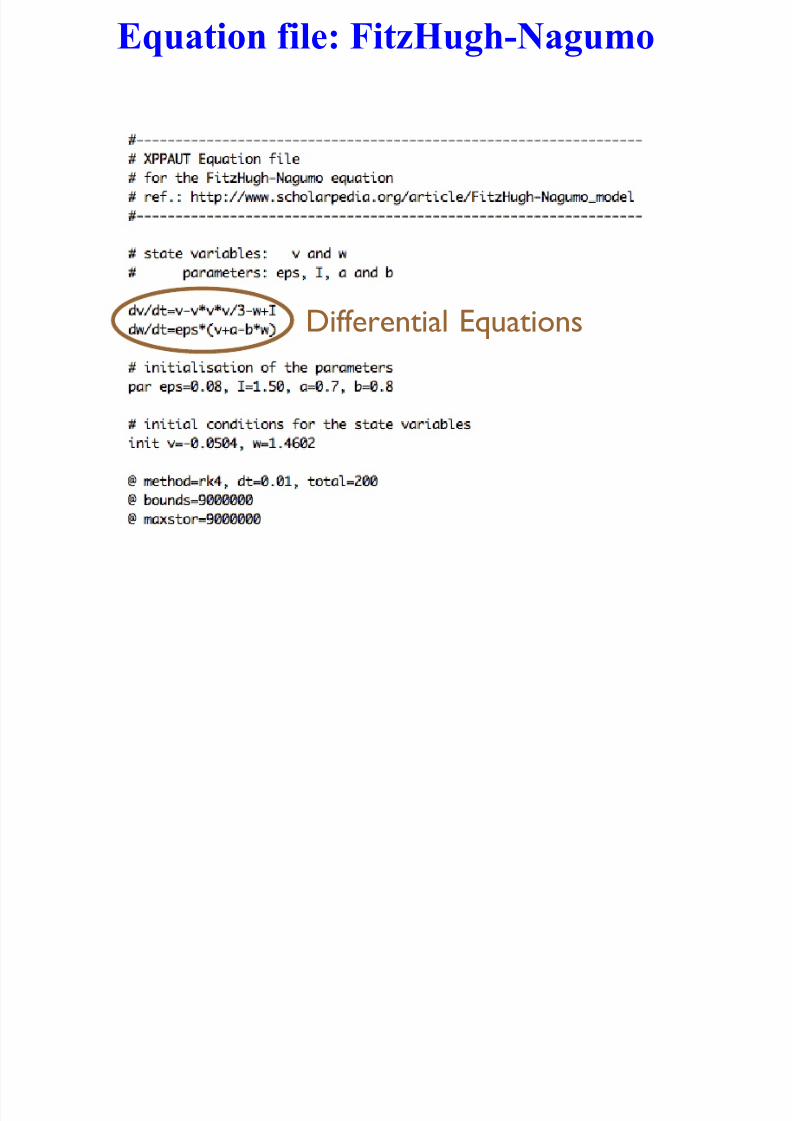
Differential Equations
Equation file: FitzHugh-Nagumo
7/27/2019 Xppaut Roscoff
http://slidepdf.com/reader/full/xppaut-roscoff 105/165
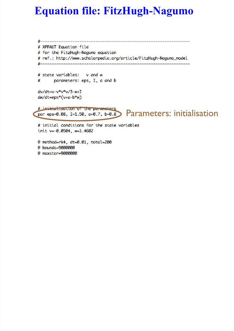
Parameters: initialisation
Equation file: FitzHugh-Nagumo
7/27/2019 Xppaut Roscoff
http://slidepdf.com/reader/full/xppaut-roscoff 106/165
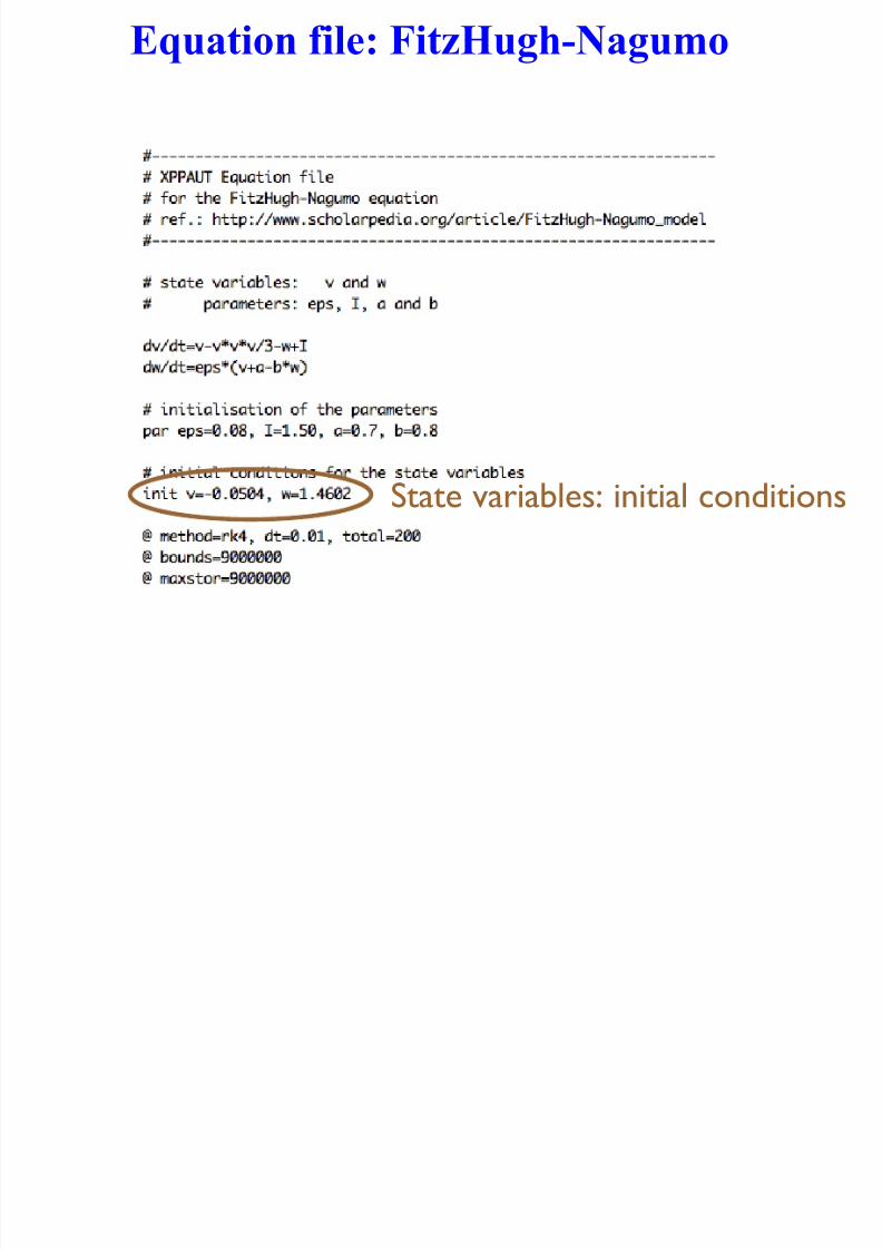
State variables: initial conditions
Equation file: FitzHugh-Nagumo

7/27/2019 Xppaut Roscoff
http://slidepdf.com/reader/full/xppaut-roscoff 107/165
Numerical accuracy
XPP-part

7/27/2019 Xppaut Roscoff
http://slidepdf.com/reader/full/xppaut-roscoff 108/165
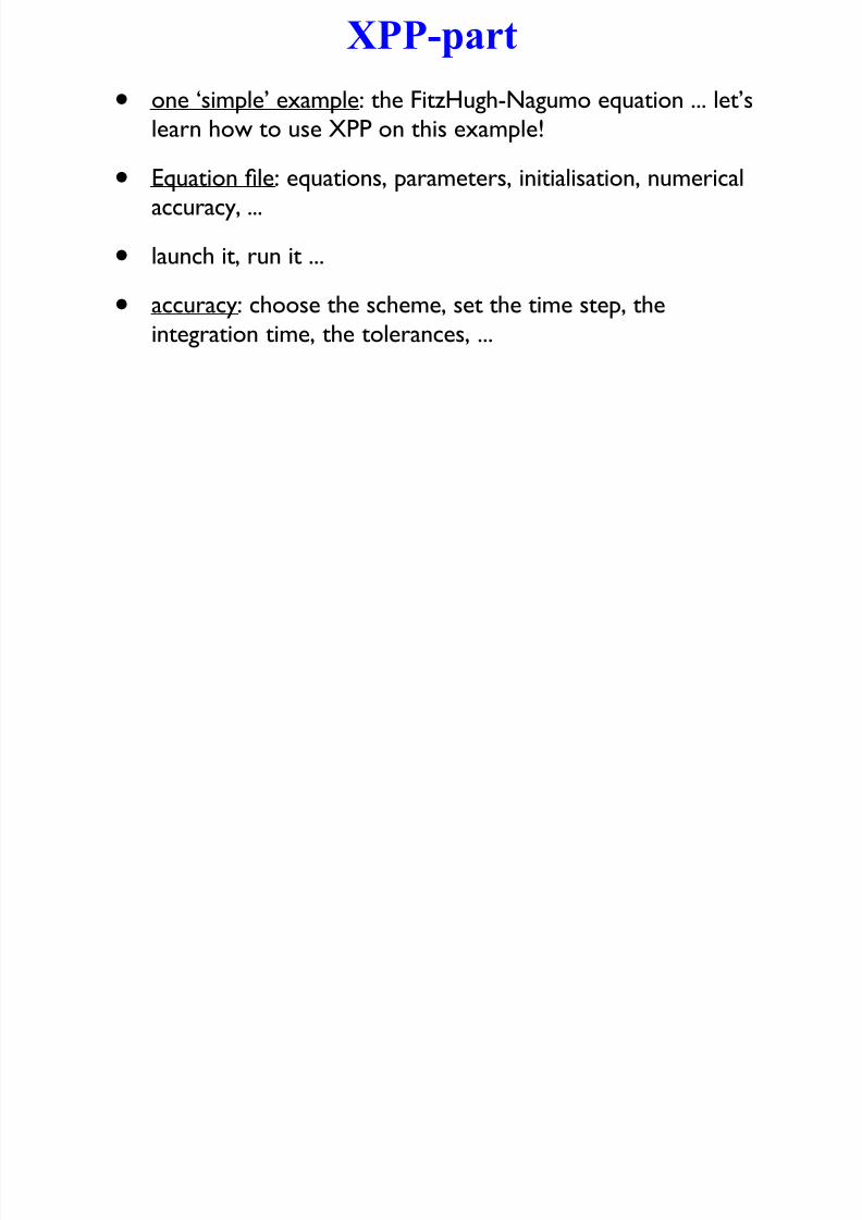
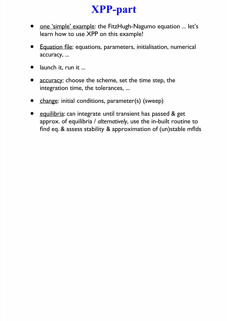
• one ‘simple’ example: the FitzHugh-Nagumo equation ... let’s
learn how to use XPP on this example!
• Equation file: equations, parameters, initialisation, numericalaccuracy, ...
• launch it, run it ...
• accuracy: choose the scheme, set the time step, theintegration time, the tolerances, ...
• change: initial conditions, parameter(s) (sweep)
• equilibria: can integrate until transient has passed & get
approx. of equilibria / alternatively , use the in-built routine tofind eq. & assess stability & approximation of (un)stable mflds
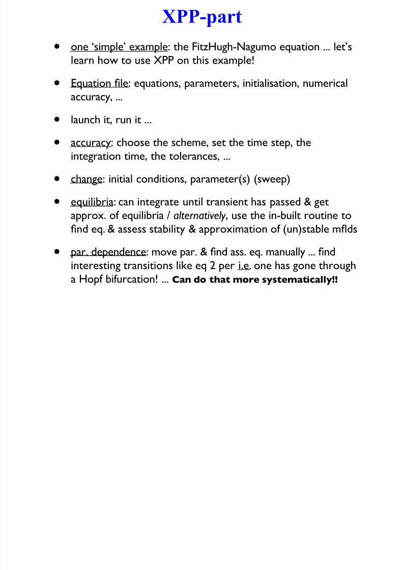
• par. dependence: move par. & find ass. eq. manually ... find
interesting transitions like eq 2 per i.e. one has gone through
a Hopf bifurcation! ... Can do that more systematically!!
XPP-part

7/27/2019 Xppaut Roscoff
http://slidepdf.com/reader/full/xppaut-roscoff 109/165
• one ‘simple’ example: the FitzHugh-Nagumo equation ... let’s
learn how to use XPP on this example!
• Equation file: equations, parameters, initialisation, numericalaccuracy, ...
• launch it, run it ...
•accuracy: choose the scheme, set the time step, the
integration time, the tolerances, ...
• change: initial conditions, parameter(s) (sweep)
• equilibria: can integrate until transient has passed & get
approx. of equilibria / alternatively , use the in-built routine tofind eq. & assess stability & approximation of (un)stable mflds
• par. dependence: move par. & find ass. eq. manually ... find
interesting transitions like eq 2 per i.e. one has gone through
a Hopf bifurcation! ... Can do that more systematically!!
XPP-part

7/27/2019 Xppaut Roscoff
http://slidepdf.com/reader/full/xppaut-roscoff 110/165
• one ‘simple’ example: the FitzHugh-Nagumo equation ... let’s
learn how to use XPP on this example!
• Equation file: equations, parameters, initialisation, numericalaccuracy, ...
• launch it, run it ...
•accuracy: choose the scheme, set the time step, the
integration time, the tolerances, ...
• change: initial conditions, parameter(s) (sweep)
• equilibria: can integrate until transient has passed & get
approx. of equilibria / alternatively , use the in-built routine tofind eq. & assess stability & approximation of (un)stable mflds
• par. dependence: move par. & find ass. eq. manually ... find
interesting transitions like eq 2 per i.e. one has gone through
a Hopf bifurcation! ... Can do that more systematically!!

7/27/2019 Xppaut Roscoff
http://slidepdf.com/reader/full/xppaut-roscoff 111/165
XPP-part
7/27/2019 Xppaut Roscoff
http://slidepdf.com/reader/full/xppaut-roscoff 112/165
• one ‘simple’ example: the FitzHugh-Nagumo equation ... let’s
learn how to use XPP on this example!
• Equation file: equations, parameters, initialisation, numericalaccuracy, ...
• launch it, run it ...
•accuracy: choose the scheme, set the time step, the
integration time, the tolerances, ...
• change: initial conditions, parameter(s) (sweep)
• equilibria: can integrate until transient has passed & get
approx. of equilibria / alternatively , use the in-built routine tofind eq. & assess stability & approximation of (un)stable mflds
• par. dependence: move par. & find ass. eq. manually ... find
interesting transitions like eq 2 per i.e. one has gone through
a Hopf bifurcation! ... Can do that more systematically!!
XPP-part

7/27/2019 Xppaut Roscoff
http://slidepdf.com/reader/full/xppaut-roscoff 113/165
• one ‘simple’ example: the FitzHugh-Nagumo equation ... let’s
learn how to use XPP on this example!
• Equation file: equations, parameters, initialisation, numericalaccuracy, ...
• launch it, run it ...
•accuracy: choose the scheme, set the time step, the
integration time, the tolerances, ...
• change: initial conditions, parameter(s) (sweep)
• equilibria: can integrate until transient has passed & get
approx. of equilibria / alternatively , use the in-built routine tofind eq. & assess stability & approximation of (un)stable mflds
• par. dependence: move par. & find ass. eq. manually ... find
interesting transitions like eq 2 per i.e. one has gone through
a Hopf bifurcation! ... Can do that more systematically!!
7/27/2019 Xppaut Roscoff
http://slidepdf.com/reader/full/xppaut-roscoff 114/165
7/27/2019 Xppaut Roscoff
http://slidepdf.com/reader/full/xppaut-roscoff 115/165
7/27/2019 Xppaut Roscoff
http://slidepdf.com/reader/full/xppaut-roscoff 116/165
Let’s launch it and try!
7/27/2019 Xppaut Roscoff
http://slidepdf.com/reader/full/xppaut-roscoff 117/165
We’re now going to learn XPP
with the FitzHugh-Nagumoequation ...
AUT-part
7/27/2019 Xppaut Roscoff
http://slidepdf.com/reader/full/xppaut-roscoff 118/165
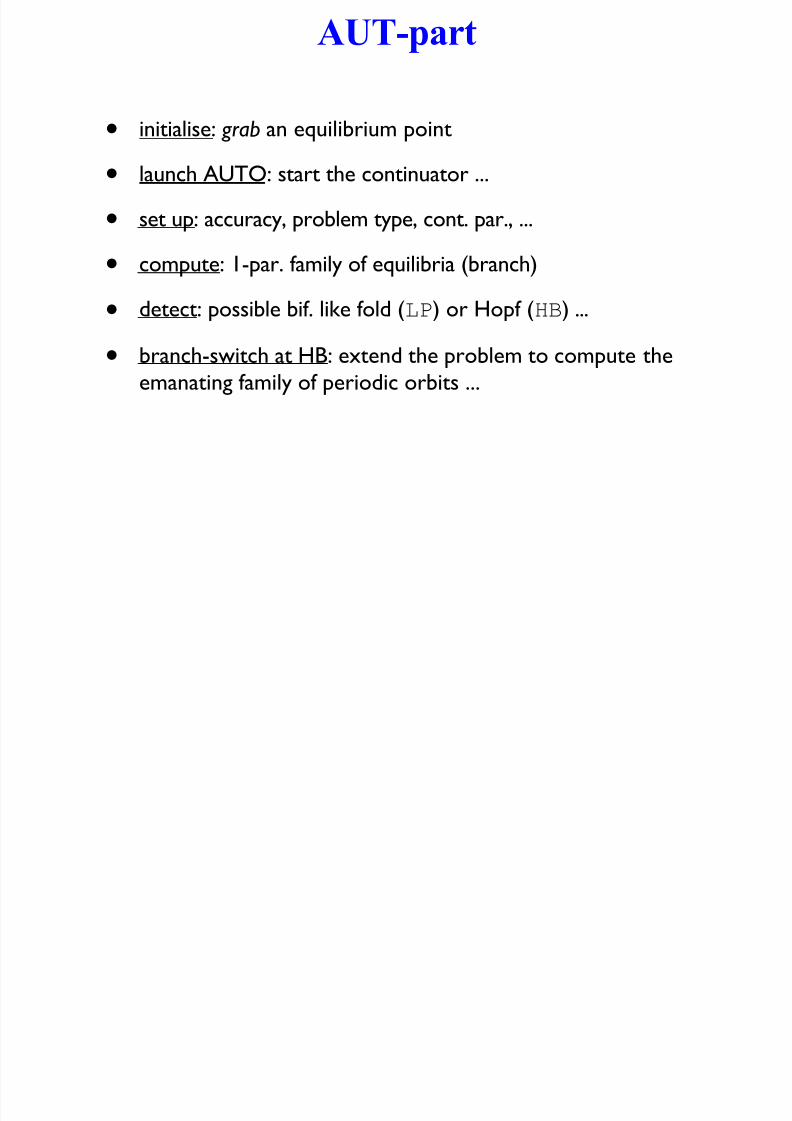
• initialise: grab an equilibrium point
• launch AUTO: start the continuator ...
• set up: accuracy, problem type, cont. par., ...
• compute: 1-par. family of equilibria (branch)
• detect: possible bif. like fold (LP) or Hopf (HB) ...
• branch-switch at HB: extend the problem to compute the
emanating family of periodic orbits ...

7/27/2019 Xppaut Roscoff
http://slidepdf.com/reader/full/xppaut-roscoff 119/165
Let’s launch it and try!

7/27/2019 Xppaut Roscoff
http://slidepdf.com/reader/full/xppaut-roscoff 120/165
Let’s launch it and try!

7/27/2019 Xppaut Roscoff
http://slidepdf.com/reader/full/xppaut-roscoff 121/165

7/27/2019 Xppaut Roscoff
http://slidepdf.com/reader/full/xppaut-roscoff 122/165
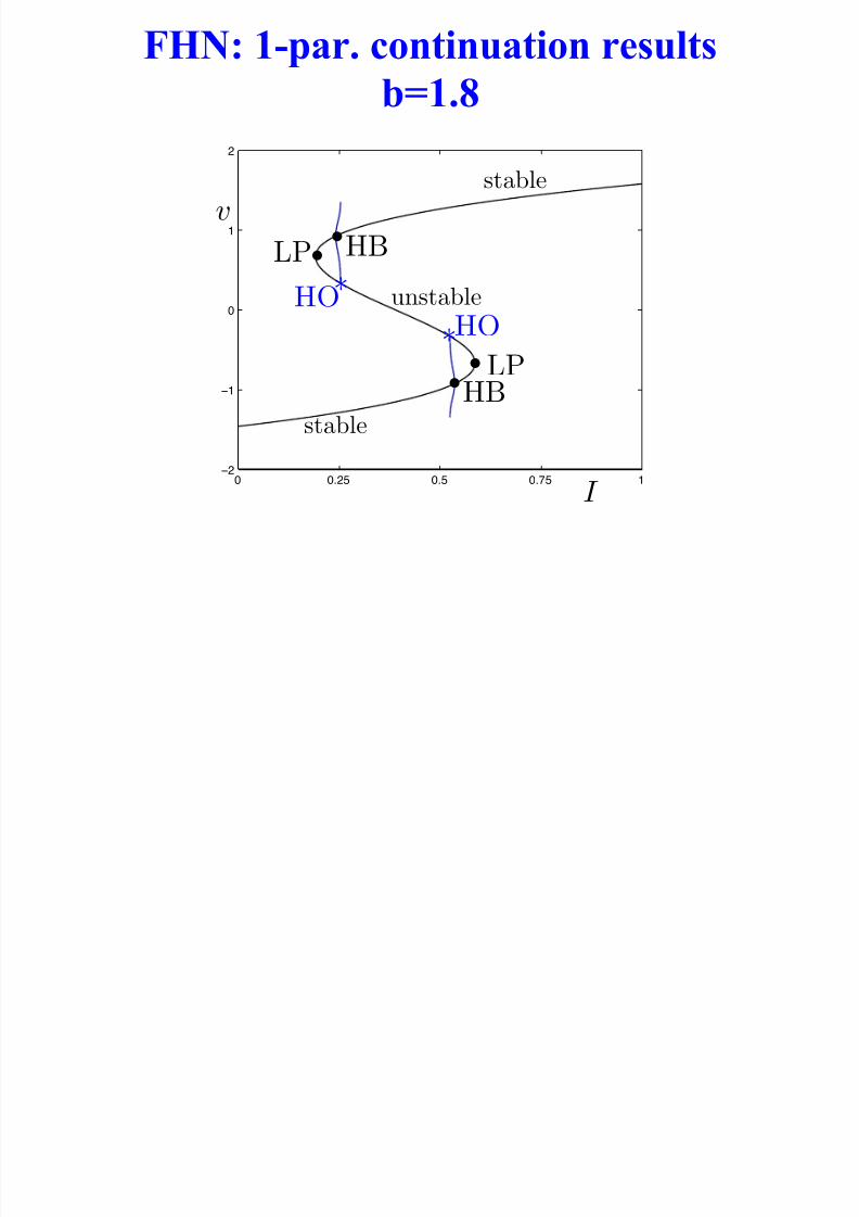
FHN: 1-par. continuation results
b=1 8
7/27/2019 Xppaut Roscoff
http://slidepdf.com/reader/full/xppaut-roscoff 123/165
! !"#$ !"$ !"%$ &−#
−&
!
&
#
b=1.8
I
v
•
•HB
HB
stable
unstable
stable
•
•
LP
LP
∗
∗
HO
HO

7/27/2019 Xppaut Roscoff
http://slidepdf.com/reader/full/xppaut-roscoff 124/165

7/27/2019 Xppaut Roscoff
http://slidepdf.com/reader/full/xppaut-roscoff 125/165

7/27/2019 Xppaut Roscoff
http://slidepdf.com/reader/full/xppaut-roscoff 126/165
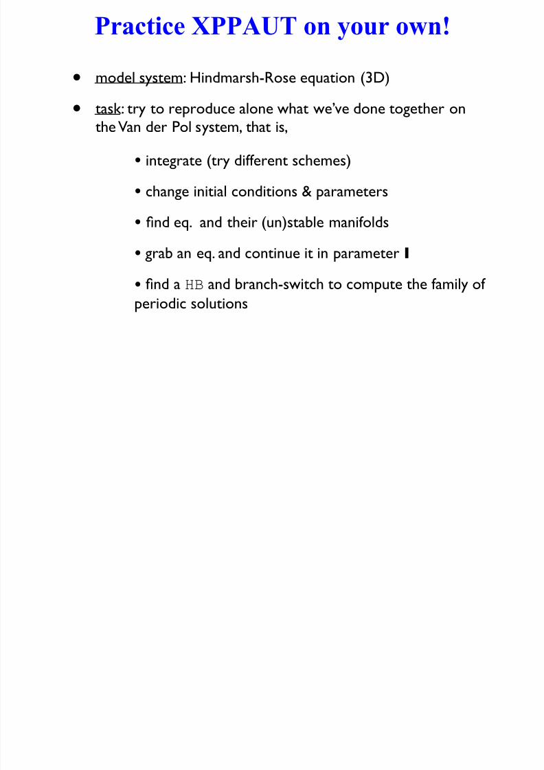
Part III: XPPAUT
- practice it yourself -
7/27/2019 Xppaut Roscoff
http://slidepdf.com/reader/full/xppaut-roscoff 127/165
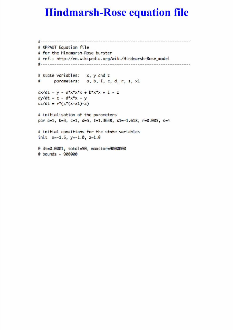
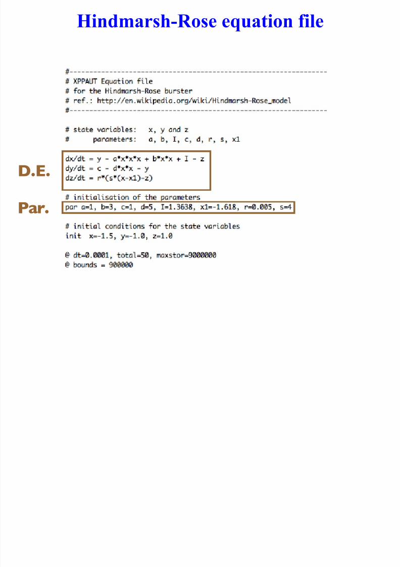
Hindmarsh-Rose equation file
7/27/2019 Xppaut Roscoff
http://slidepdf.com/reader/full/xppaut-roscoff 128/165
D.E.
7/27/2019 Xppaut Roscoff
http://slidepdf.com/reader/full/xppaut-roscoff 129/165

7/27/2019 Xppaut Roscoff
http://slidepdf.com/reader/full/xppaut-roscoff 130/165
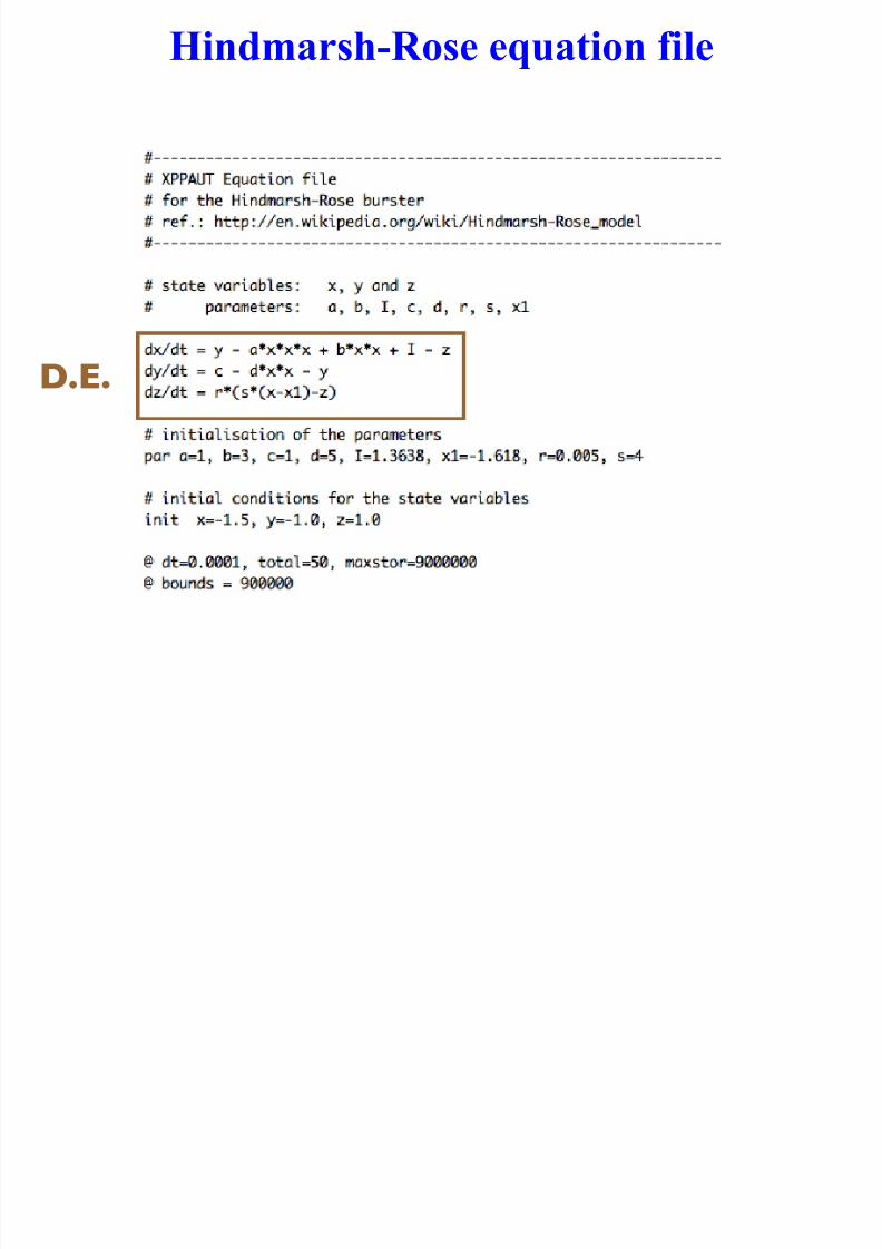
Hindmarsh-Rose equation file

7/27/2019 Xppaut Roscoff
http://slidepdf.com/reader/full/xppaut-roscoff 131/165
D.E.
Par.
I.C.
Num.
7/27/2019 Xppaut Roscoff
http://slidepdf.com/reader/full/xppaut-roscoff 132/165

7/27/2019 Xppaut Roscoff
http://slidepdf.com/reader/full/xppaut-roscoff 133/165

7/27/2019 Xppaut Roscoff
http://slidepdf.com/reader/full/xppaut-roscoff 134/165

7/27/2019 Xppaut Roscoff
http://slidepdf.com/reader/full/xppaut-roscoff 135/165

7/27/2019 Xppaut Roscoff
http://slidepdf.com/reader/full/xppaut-roscoff 136/165
7/27/2019 Xppaut Roscoff
http://slidepdf.com/reader/full/xppaut-roscoff 137/165
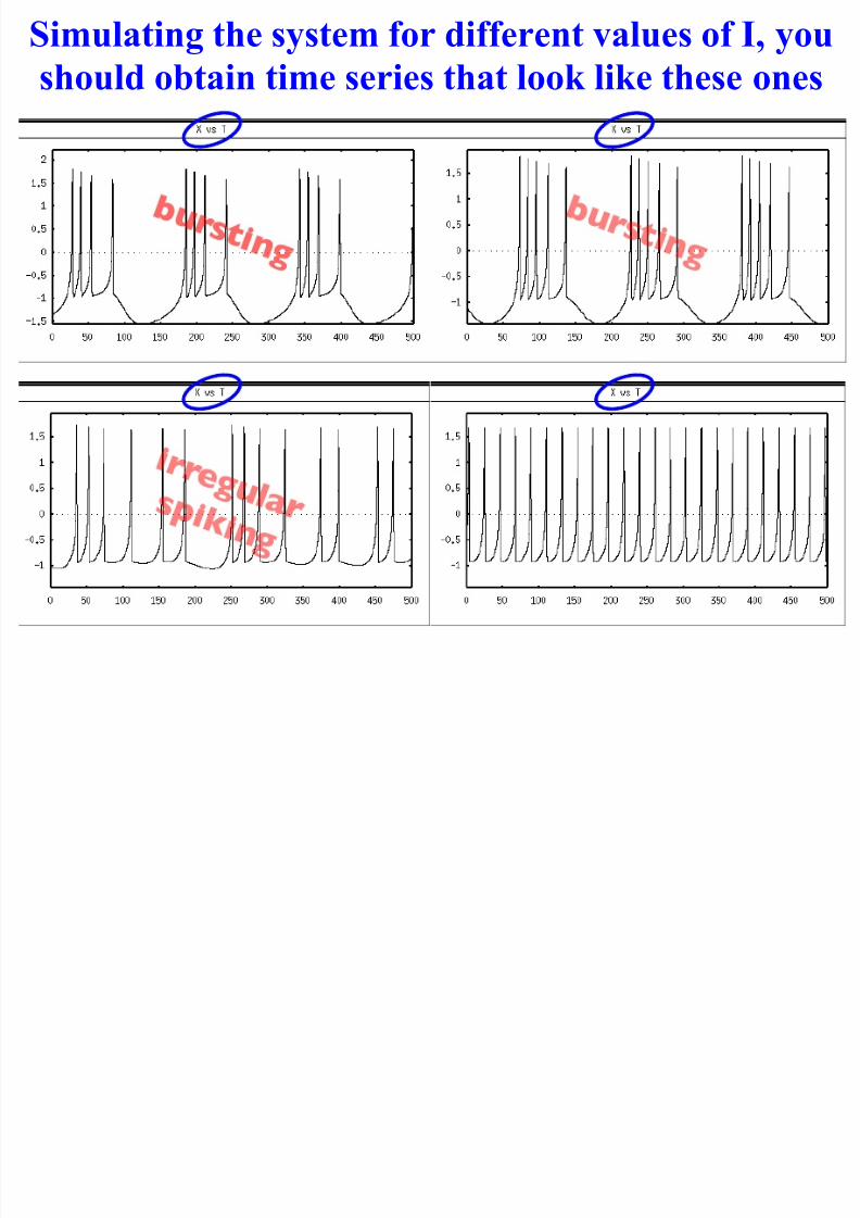
Simulating the system for different values of I, youshould obtain time series that look like these ones

7/27/2019 Xppaut Roscoff
http://slidepdf.com/reader/full/xppaut-roscoff 138/165
You should obtain a bifurcation
diagram that looks like this one

7/27/2019 Xppaut Roscoff
http://slidepdf.com/reader/full/xppaut-roscoff 139/165
diagram that looks like this one
! " #$ %# %&
−%
−!'"(
!'(
#'"(
)
I
x••
•
•
HB
HB HB
HB

7/27/2019 Xppaut Roscoff
http://slidepdf.com/reader/full/xppaut-roscoff 140/165

7/27/2019 Xppaut Roscoff
http://slidepdf.com/reader/full/xppaut-roscoff 141/165
References
XPPAUT
7/27/2019 Xppaut Roscoff
http://slidepdf.com/reader/full/xppaut-roscoff 142/165
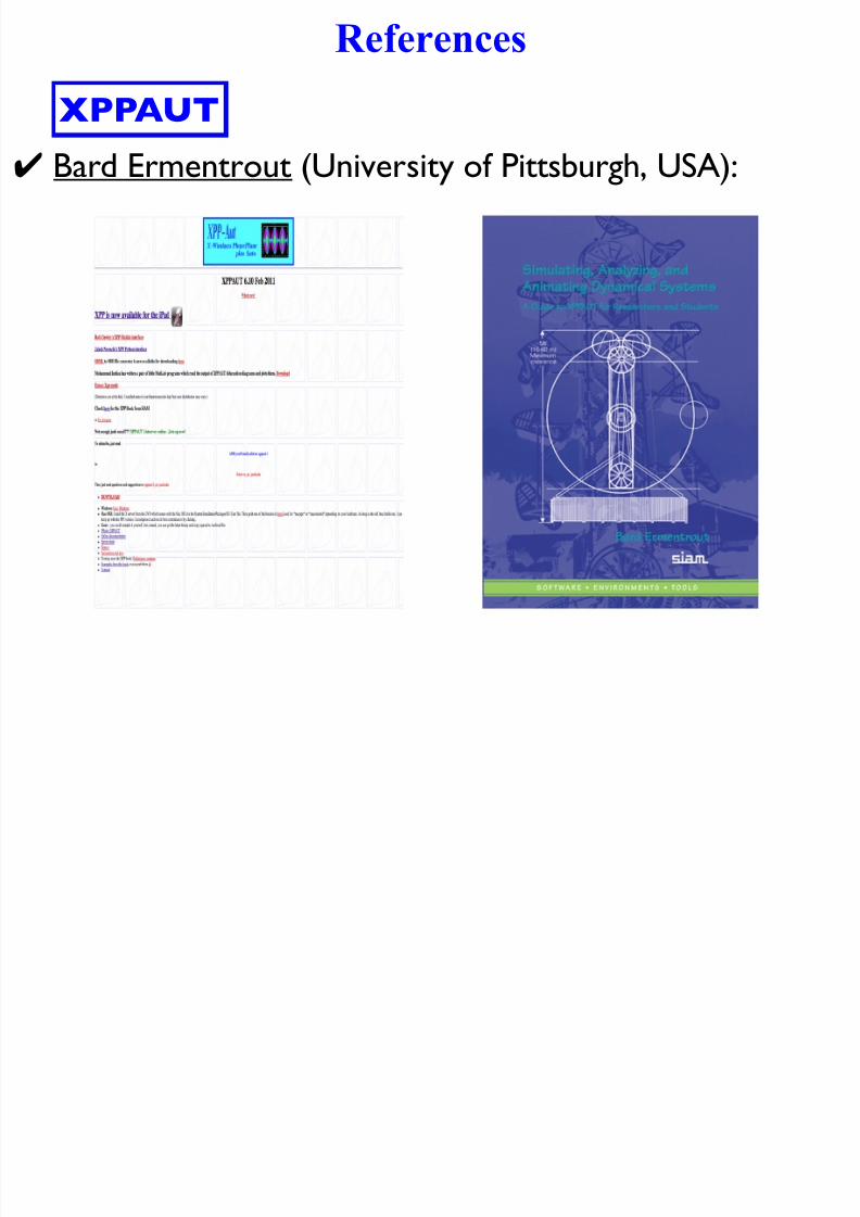
% Bard Ermentrout (University of Pittsburgh, USA):
XPPAUT
7/27/2019 Xppaut Roscoff
http://slidepdf.com/reader/full/xppaut-roscoff 143/165

7/27/2019 Xppaut Roscoff
http://slidepdf.com/reader/full/xppaut-roscoff 144/165
7/27/2019 Xppaut Roscoff
http://slidepdf.com/reader/full/xppaut-roscoff 145/165

7/27/2019 Xppaut Roscoff
http://slidepdf.com/reader/full/xppaut-roscoff 146/165

7/27/2019 Xppaut Roscoff
http://slidepdf.com/reader/full/xppaut-roscoff 147/165

7/27/2019 Xppaut Roscoff
http://slidepdf.com/reader/full/xppaut-roscoff 148/165
References ...
ODEs & Bifurcations

7/27/2019 Xppaut Roscoff
http://slidepdf.com/reader/full/xppaut-roscoff 149/165
ODEs & Bifurcations
(‘Tutorials’ & ‘Software’ sections)
http://www.bio.vu.nl/thb/research/project/globif/
(MathDoctorMitchell’s Channel)
References ...
ODEs & Bifurcations
7/27/2019 Xppaut Roscoff
http://slidepdf.com/reader/full/xppaut-roscoff 150/165
ODEs & Bifurcations
(‘Tutorials’ & ‘Software’ sections)
http://www.bio.vu.nl/thb/research/project/globif/
(MathDoctorMitchell’s Channel)

7/27/2019 Xppaut Roscoff
http://slidepdf.com/reader/full/xppaut-roscoff 151/165
Beyond XPPAUT!

7/27/2019 Xppaut Roscoff
http://slidepdf.com/reader/full/xppaut-roscoff 152/165
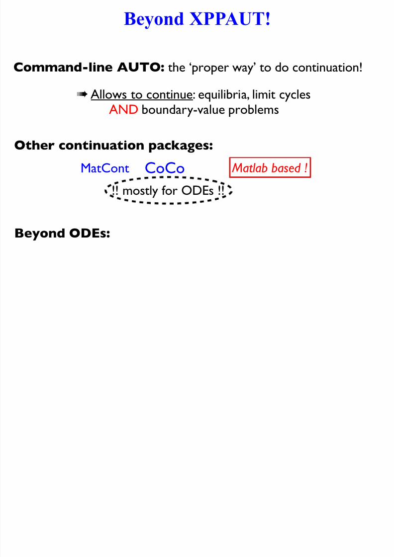
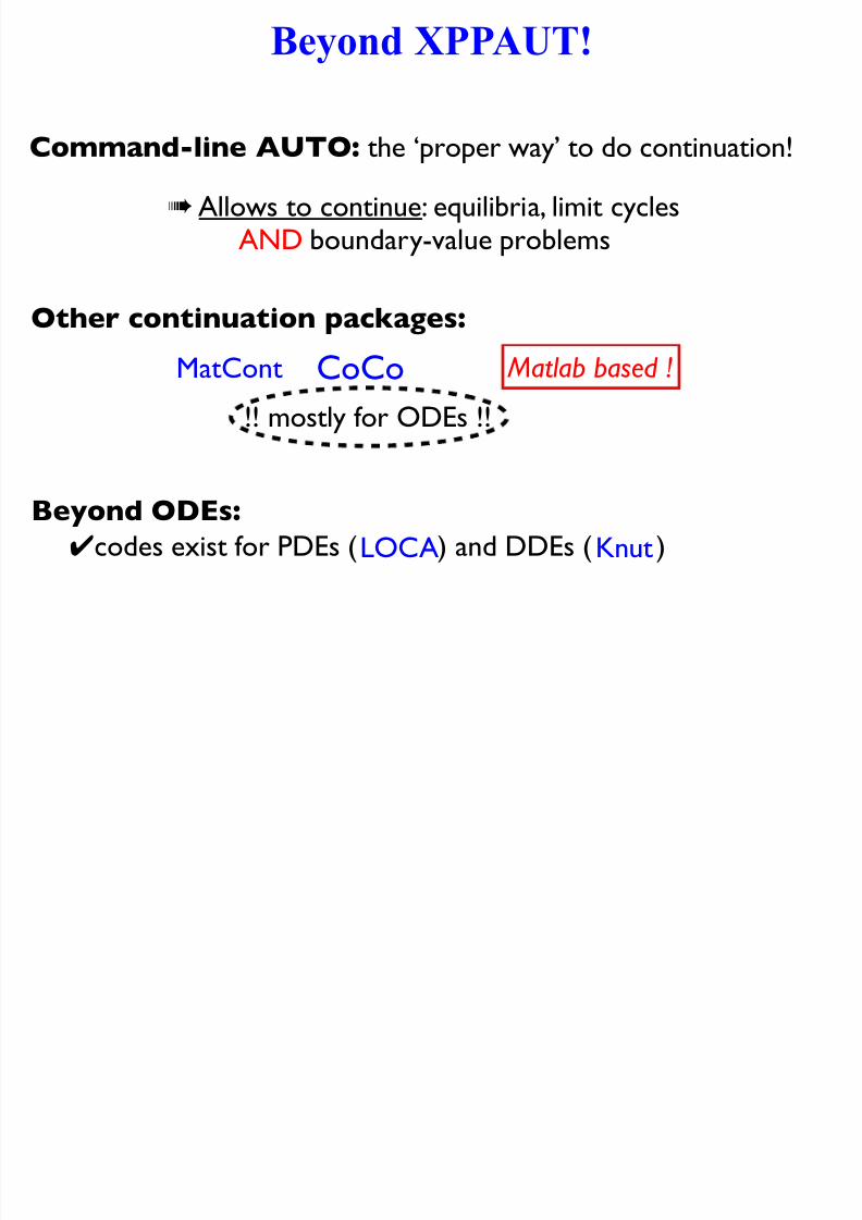
Command-line AUTO: the ‘proper way’ to do continuation!
Beyond XPPAUT!
7/27/2019 Xppaut Roscoff
http://slidepdf.com/reader/full/xppaut-roscoff 153/165
Command-line AUTO: the ‘proper way’ to do continuation!
! Allows to continue: equilibria, limit cyclesAND boundary-value problems
Beyond XPPAUT!

7/27/2019 Xppaut Roscoff
http://slidepdf.com/reader/full/xppaut-roscoff 154/165
Command-line AUTO: the ‘proper way’ to do continuation!
! Allows to continue: equilibria, limit cyclesAND boundary-value problems
Other continuation packages: MatCont Matlab based !CoCo
Beyond XPPAUT!

7/27/2019 Xppaut Roscoff
http://slidepdf.com/reader/full/xppaut-roscoff 155/165
Command-line AUTO: the ‘proper way’ to do continuation!
! Allows to continue: equilibria, limit cyclesAND boundary-value problems
Other continuation packages: MatCont Matlab based !
!! mostly for ODEs !!
CoCo
Beyond XPPAUT!
7/27/2019 Xppaut Roscoff
http://slidepdf.com/reader/full/xppaut-roscoff 156/165
Command-line AUTO: the ‘proper way’ to do continuation!
! Allows to continue: equilibria, limit cyclesAND boundary-value problems
Other continuation packages: MatCont Matlab based !
Beyond ODEs:
!! mostly for ODEs !!
CoCo
Beyond XPPAUT!
7/27/2019 Xppaut Roscoff
http://slidepdf.com/reader/full/xppaut-roscoff 157/165
Command-line AUTO: the ‘proper way’ to do continuation!
! Allows to continue: equilibria, limit cyclesAND boundary-value problems
Other continuation packages: MatCont Matlab based !
Beyond ODEs:
%codes exist for PDEs ( ) and DDEs ( )
!! mostly for ODEs !!
CoCo
LOCA Knut

7/27/2019 Xppaut Roscoff
http://slidepdf.com/reader/full/xppaut-roscoff 158/165
References
AUTO - 07p

7/27/2019 Xppaut Roscoff
http://slidepdf.com/reader/full/xppaut-roscoff 159/165
p

7/27/2019 Xppaut Roscoff
http://slidepdf.com/reader/full/xppaut-roscoff 160/165
References
AUTO - 07p

7/27/2019 Xppaut Roscoff
http://slidepdf.com/reader/full/xppaut-roscoff 161/165
% Eusebius Doedel (Concordia University, Montreal):
p
References
AUTO - 07p

7/27/2019 Xppaut Roscoff
http://slidepdf.com/reader/full/xppaut-roscoff 162/165
% Eusebius Doedel (Concordia University, Montreal):
p
References
AUTO - 07p

7/27/2019 Xppaut Roscoff
http://slidepdf.com/reader/full/xppaut-roscoff 163/165
% Eusebius Doedel (Concordia University, Montreal):
p
http://www2 imperial ac uk/~jswlamb/LDSG/grad0506/auto course htm

7/27/2019 Xppaut Roscoff
http://slidepdf.com/reader/full/xppaut-roscoff 164/165
Thanks for your attention!

7/27/2019 Xppaut Roscoff
http://slidepdf.com/reader/full/xppaut-roscoff 165/165
Thanks for your attention!
... questions?


