XQVFKRWHQ - TU Delft

TurbomachineryAnalysis and DesignUsing Body-ForceModeling in SU2

E. C. BunschotenMaster Thesis ReportAerospace Propulsion and Power Engineering15-10-2020

TurbomachineryAnalysis andDesign UsingBody-Force

Modeling in SU2by

E. C. Bunschotento obtain the degree of Master of Scienceat the Delft University of Technology,

to be defended publicly on Thursday October 15, 2020 at 14:00

Student number: 4455584Project duration: January 28, 2020 – October 15, 2020Thesis committee: Prof. dr. ir. M. Pini, TU Delft, supervisor

ir. N. Anand, TU Delft, supervisorProf. dr. ir. P. Colonna TU Delftdr. R. P. Dwight TU Delft

PrefaceThis report represents the final research project conducted in the Master curriculum of AerospacePropulsion and Power Engineering. This research report is intended for those who seek insightin the workings of body-force models, the implementation of Thollets body-force model intoSU2 and its capabilities. Information regarding the implementation can be found in Chapter 3,Section 3.3. Additionally, readers who are interested in using body-force modeling in a designcontext could find inspiration in this document and utilize the methods posed. For those inter-ested in the design analysis workflow, an example analysis case can be found in Appendix A.Here, a GitHub link to the method can also be found.Including literature study, it has taken about a year to complete this research, in which theworld has changed drastically. The situation regarding the global pandemic caused several de-lays and hindered communication, as physical meetings with my supervisors were prohibited.Despite these difficulties, I always felt well-supported. Matteo Pini, the professor who guidedme through the research was a joy to work with. He was always curious regarding updates andoffered valuable advice when major decisions had to be made regarding the research. Specialthanks also goes to Nitish Anand, a PHD candidate within the Propulsion and Power researchgroup at TU Delft. His expertise in the SU2 code structure was of crucial help while implement-ing the body-force model into SU2. Along side that, he was (nearly) always available for videochat to resolve technical issues, which was highly appreciated. Finally, my gratitude goes toWilliam Thollet and Luis Lopez de Vega, of Airbus. They originally developed the body-forcemodel used in this thesis and offered their advice regarding the implementation of it.

i

AbstractAs aircraft manufacturers push for better fuel economy, novel aircraft concepts, like the propul-sive fuselage concept have emerged. One of the prime component of such concepts is theboundary layer ingestion (BLI) engine. Such engine operates by ingesting the low-momentumfluid emerging from the surface of the aircraft fuselage which enables to enhance its propulsiveefficiency. The design of a BLI engine is fundamentally different than that of a conventionalaircraft engine as the BLI fan experiences distorted airflow at every revolution. Therefore, whenits performance are analyzed by means of CFD, single passage simulations become insufficientto represent the flow characteristics. and extremely expensive simulation of the entire annulusbecome necessary for analysis and design purposes. Especially during conceptual design, whereseveral BLI engine configurations must be investigated in combination with their airframe inte-gration, new reduced-order methods are required to alleviate the computational burden whileretaining a sufficient level of accuracy.

An alternative, computationally efficient approach capable of coping with the full-annulus simulation is the well-established body-force modelling (BFM). BFM is a techniquethrough which the physical blade rows are replaced by a volumetric force field which mimics theflow turning imparted by the physical blade rows. Thanks to this simplification, BFM does notrequire the physical blades to be accurately reproduced in the mesh, thus offering substantialcomputational cost reduction. Due to the associated gains in computational efficiency, thismethod is commonly used for the analysis and off-design performance prediction of full-annulusgeometries, which are computationally demanding through conventional methods. Althoughthe method has been established for analysis purposes, its capability as a design tool was neverassessed.

Implementation of BFM in a CFD code that can be automatically differentiated toattain design sensitivities via the adjoint method may enable efficient BFM-based design ofcomplex engine configurations.

In this research, the BFM model originally developed by Ref. [1] and improved by Ref.[2] was implemented into open-source CFD software SU2, which is equipped with a discreteadjoint solver based on operator overloading. In addition, parallel force and a metal blockagesource term were added to the existing formulation to increase the fidelity of the BFM. Theimplementation was validated by comparing the results obtained from the BFM and the physicalblade computation on an exemplary axial turbine test case.

The results show that the BFM was capable of providing static and stagnation pressureand temperature trends with an accuracy of approximately 94%. Furthermore, the absolute flowdeflection by the stator and rotor rows were found to deviate by 5 and 17. The BFM wasfound to be 3 orders of magnitude faster than the equivalent physical blade computation.

ii

Table of Contents

Preface i

Abstract ii

List of Symbols ii

List of Figures iv

List of Tables v

1 Introduction 11.1 Motivation and Research Objective . . . . . . . . . . . . . . . . . . . . . . . . . . 11.2 Original Contributions . . . . . . . . . . . . . . . . . . . . . . . . . . . . . . . . . 21.3 Outline . . . . . . . . . . . . . . . . . . . . . . . . . . . . . . . . . . . . . . . . . 3

2 Background Knowledge 42.1 Body-force modeling . . . . . . . . . . . . . . . . . . . . . . . . . . . . . . . . . . 42.2 Applications and limitations of body-force modeling . . . . . . . . . . . . . . . . 72.3 Original BFM implementation in SU2 . . . . . . . . . . . . . . . . . . . . . . . . 82.4 Thollet’s BFM . . . . . . . . . . . . . . . . . . . . . . . . . . . . . . . . . . . . . 10

3 Research Methodology 133.1 Ray-Cast Interpolation . . . . . . . . . . . . . . . . . . . . . . . . . . . . . . . . . 133.2 3D BFM transformation . . . . . . . . . . . . . . . . . . . . . . . . . . . . . . . . 143.3 BFM solver structure . . . . . . . . . . . . . . . . . . . . . . . . . . . . . . . . . . 163.4 Automated Workflow for BFM Computations . . . . . . . . . . . . . . . . . . . . 16

4 BFM Verification 194.1 Verification of Parallel Force Implementation . . . . . . . . . . . . . . . . . . . . 194.2 Metal Blockage Model Verification . . . . . . . . . . . . . . . . . . . . . . . . . . 21

5 BFM Case Study 265.1 Aachen Turbine Blade Computation Setup . . . . . . . . . . . . . . . . . . . . . . 265.2 BFM Computation Setup . . . . . . . . . . . . . . . . . . . . . . . . . . . . . . . 28

6 Results 306.1 Verification of Parallel Force Implementation . . . . . . . . . . . . . . . . . . . . 306.2 Verification of Metal Blockage Model Implementation . . . . . . . . . . . . . . . 326.3 Aachen Turbine Case Study Results . . . . . . . . . . . . . . . . . . . . . . . . . 36

6.3.1 Results as a Function of Axial Node Density . . . . . . . . . . . . . . . . 366.3.2 Tangential node count study . . . . . . . . . . . . . . . . . . . . . . . . . 496.3.3 Grid convergence . . . . . . . . . . . . . . . . . . . . . . . . . . . . . . . . 49

7 Conclusions 52

8 Final Remarks and Perspectives 548.1 Final Remarks . . . . . . . . . . . . . . . . . . . . . . . . . . . . . . . . . . . . . 548.2 Perspectives . . . . . . . . . . . . . . . . . . . . . . . . . . . . . . . . . . . . . . . 54

A Design Work Flow Demonstration 56A.1 Design variable selection . . . . . . . . . . . . . . . . . . . . . . . . . . . . . . . . 56

iii

B Radial section data 60

References 63

List of SymbolsAbbreviations

ADM Actuator Disc Model

BFM Body-Force Model

BLI Boundary-Layer Ingestion

NS Navier-Stokes

RANS Reynolds Averaged Navier-Stokes

SU2 Stanford University Unstructured

TSFC Thrust Specific Fuel Consumption

URANS Unsteady Reynolds Averaged Navier-Stokes

Roman Symbols

b Blockage factor [-]

cp Specific enthalpy [J kg−1 K−1]

F Body-force [kg m−2 s−2]

f Body-force, momentum vector

h Enthalpy [J kg−1 K−1]

n Camber normal vector component

Nx Node count in axial direction [-]

R∗ Degree of reaction [-]

T Temperature [K]

u Absolute velocity [m s−1]

R Gas constant [J kg−1 K−1]

Greek Symbols

β Blade metal angle []

γ Specific heat ratio [-]

Ω Rotation rate [rad/s]

φ Flow coefficient [-]

ψ Work coefficient [-]

ξ Vortex-free twist parameter [-]

Subscripts

θ Tangential

i

ax Axial

n Normal

p Parallel

r Radial

s Static conditions

t Stagnation conditions

hub At height of the hub

LE At the leading edge

shroud At height of the shroud

TE At the trailing edge

ii

List of Figures

2.1 Different blade shapes interpolated to the same mesh . . . . . . . . . . . . . . . . 72.2 Hall’s BFM illustration . . . . . . . . . . . . . . . . . . . . . . . . . . . . . . . . 92.3 Definition of effective pitch and blade pitch . . . . . . . . . . . . . . . . . . . . . 112.4 Illustration of the parallel body-force component . . . . . . . . . . . . . . . . . . 12

3.1 Illustration of the ray-casting principle . . . . . . . . . . . . . . . . . . . . . . . . 143.2 SU2 BFM solver structure . . . . . . . . . . . . . . . . . . . . . . . . . . . . . . . 163.3 BFM preprocessing workflow diagram . . . . . . . . . . . . . . . . . . . . . . . . 17

4.1 axial-radial slice of parallel force verification domain . . . . . . . . . . . . . . . . 214.2 Prismatic cross section used for metal blockage verification . . . . . . . . . . . . 224.3 3D mesh used for the blockage verification blade computation . . . . . . . . . . . 234.4 Axial-tangential slice of blade computation domain . . . . . . . . . . . . . . . . . 244.5 Axial-radial slice of blade computation domain . . . . . . . . . . . . . . . . . . . 244.6 Axial-radial slice of BFM computation domain . . . . . . . . . . . . . . . . . . . 244.7 Axial-tangential slice of BFM computation domain at mid-span . . . . . . . . . . 25

5.1 Aachen turbine flow domain . . . . . . . . . . . . . . . . . . . . . . . . . . . . . . 265.2 Aachen stator cross section . . . . . . . . . . . . . . . . . . . . . . . . . . . . . . 275.3 Aachen rotor cross section . . . . . . . . . . . . . . . . . . . . . . . . . . . . . . . 275.4 Axial node count definition . . . . . . . . . . . . . . . . . . . . . . . . . . . . . . 285.5 Tangential node count definition . . . . . . . . . . . . . . . . . . . . . . . . . . . 29

6.1 Density residual convergence trend . . . . . . . . . . . . . . . . . . . . . . . . . . 306.2 Comparison between entropy gradient and parallel force . . . . . . . . . . . . . . 316.3 Comparison between pressure gradient and parallel force . . . . . . . . . . . . . . 316.4 Comparison between pressure gradient and parallel force with inclusion of kinetic

energy gradient . . . . . . . . . . . . . . . . . . . . . . . . . . . . . . . . . . . . . 326.5 Comparison between interpolated and analytical blockage factor distribution . . 326.6 Comparison between interpolated and analytical blockage factor distribution . . 336.7 Mach number distribution in BFM results (radius=0.2875 m) . . . . . . . . . . . 336.8 Mach number distribution in the blade computation results(radius=0.2875 m) . . 346.9 Mach number comparison between blade computation and BFM . . . . . . . . . 346.10 Mass flux comparison between blade computation and BFM . . . . . . . . . . . . 356.11 Normalized static pressure comparison between blade computation and BFM . . 356.12 Deviation between BFM mass flux and blade computation mass flux trends . . . 366.13 Convergence trend comparison between the different mesh densities . . . . . . . . 376.14 Total convergence time for each level of mesh refinement . . . . . . . . . . . . . . 376.15 Comparison of nomalized static pressure trends . . . . . . . . . . . . . . . . . . . 386.16 Static pressure deviation . . . . . . . . . . . . . . . . . . . . . . . . . . . . . . . . 396.17 Comparison of nomalized total pressure trends . . . . . . . . . . . . . . . . . . . 396.18 Stagnation pressure deviation . . . . . . . . . . . . . . . . . . . . . . . . . . . . . 406.19 Comparison of nomalized total temperature trends . . . . . . . . . . . . . . . . . 406.20 Stagnation temperature deviation . . . . . . . . . . . . . . . . . . . . . . . . . . . 416.21 Comparison of absolute flow angle trends . . . . . . . . . . . . . . . . . . . . . . 416.22 Absolute flow angle deviation . . . . . . . . . . . . . . . . . . . . . . . . . . . . . 426.23 Comparison of entropy trends . . . . . . . . . . . . . . . . . . . . . . . . . . . . . 436.24 Comparison of normalized entropy trends . . . . . . . . . . . . . . . . . . . . . . 436.25 Comparison of mass flux trends . . . . . . . . . . . . . . . . . . . . . . . . . . . . 44

iii

6.26 Mass flux deviation . . . . . . . . . . . . . . . . . . . . . . . . . . . . . . . . . . . 446.27 Axial station definition . . . . . . . . . . . . . . . . . . . . . . . . . . . . . . . . . 456.28 Radial static pressure trend between first stator and rotor . . . . . . . . . . . . . 466.29 Radial static temperature trend between first stator and rotor . . . . . . . . . . . 466.30 Radial static pressure trend between rotor and second stator . . . . . . . . . . . 476.31 Radial static temperature trend between rotor and second stator . . . . . . . . . 476.32 Radial absolute flow angle trend between the first stator and rotor . . . . . . . . 486.33 Radial absolute flow angle trend between rotor and second stator . . . . . . . . . 486.34 Static pressure Nθ comparison . . . . . . . . . . . . . . . . . . . . . . . . . . . . 496.35 Static and stagnation pressure and temperature RMS errors . . . . . . . . . . . . 506.36 Mass flux RMS error trend . . . . . . . . . . . . . . . . . . . . . . . . . . . . . . 51

A.1 Mid-span rotor cross section . . . . . . . . . . . . . . . . . . . . . . . . . . . . . . 57A.2 Mid-span stator cross section . . . . . . . . . . . . . . . . . . . . . . . . . . . . . 57A.3 Isometric view of unstructured mesh . . . . . . . . . . . . . . . . . . . . . . . . . 58A.4 Side view of unstructured mesh . . . . . . . . . . . . . . . . . . . . . . . . . . . . 58A.5 Axial, mass-flux-averaged absolute flow angle trend . . . . . . . . . . . . . . . . . 59A.6 Axial, mass-flux-averaged entropy increase trend . . . . . . . . . . . . . . . . . . 59A.7 Axial, mass-flux-averaged stagnation pressure trend . . . . . . . . . . . . . . . . 59A.8 Axial, mass-flux-averaged stagnation temperature trend . . . . . . . . . . . . . . 59

B.1 Radial absolute flow angle near the inlet . . . . . . . . . . . . . . . . . . . . . . . 60B.2 Radial absolute flow angle near the first blade leading edge . . . . . . . . . . . . 60B.3 Radial absolute flow angle in the first row gap . . . . . . . . . . . . . . . . . . . . 61B.4 Radial absolute flow angle in the second row gap . . . . . . . . . . . . . . . . . . 61B.5 Radial absolute flow angle near the last blade trailing edge . . . . . . . . . . . . 62B.6 Radial absolute flow angle near the outlet . . . . . . . . . . . . . . . . . . . . . . 62

iv

List of Tables

4.1 Parallel force verification boundary conditions . . . . . . . . . . . . . . . . . . . . 214.2 Geometric parameters of blade geometry used for blockage verification . . . . . . 224.3 Boundary conditions used for the blockage verification simulations . . . . . . . . 25

5.1 Aachen blade computation boundary conditions . . . . . . . . . . . . . . . . . . . 275.2 Aachen blade computation direct solver settings . . . . . . . . . . . . . . . . . . . 27

6.1 Tabulated total computation time for each level of mesh refinement . . . . . . . . 38

A.1 Design variable selection for demonstration compressor case . . . . . . . . . . . . 56A.2 Parablade thickness parameters . . . . . . . . . . . . . . . . . . . . . . . . . . . . 56A.3 Meangen blade geometry output . . . . . . . . . . . . . . . . . . . . . . . . . . . 57A.4 Rotor row Meangen output . . . . . . . . . . . . . . . . . . . . . . . . . . . . . . 57A.5 Stator row Meangen output . . . . . . . . . . . . . . . . . . . . . . . . . . . . . . 57

v

1 Introduction

1.1 Motivation and Research Objective

Climate change is real and global carbon emissions are one of the main causes for this crisis.This encourages transport manufacturers to rely less on hydrocarbon fuels. The aircraft in-dustry is no exception to this change. Until electric or hydrogen powered aircraft are feasible,engineers have to come up with ways to reduce the fuel consumption of future aircraft. One ofthe most effective ways to achieve this is to reduce the Thrust Specific Fuel Consumption(TSFC)of aircraft propulsors. For this, there are several options and one is to make use of BoundaryLayer Ingestion(BLI). Here, the engine is placed behind or close to the fuselage or wing, whichallows for the thrust jet to directly energize the low-momentum wake of the aircraft. This canlead to TSFC reductions of around 10% [3, 4]. A drawback of using this engine configurationis that the air flowing into the engine fan is distorted due to the fuselage boundary layer. Thisdistortion decreases the efficiency of the fan and causes flow distortions downstream of thefan, which can have negative consequences on downstream components. Current high-fidelityanalysis methodologies are capable of resolving these distortions, but are unfeasible in a designcontext due to the high associated computational costs [5]. This makes numerical design opti-mization impractical using conventional methods, as subsequent design iterations would requirevast computational resources and time. Alternative methods would have to be utilized whichrequire less computational resources, while maintaining a competent level of accuracy. Oneanalysis method which has high potential in this field is the Body-Force Model (BFM).

A BFM works by replacing the blade rows by a volumetric force field, which locally modelsthe flow turning and losses, while requiring several orders of magnitude less computation time[6] and maintaining reasonable accuracy. Various BFM’s have been developed over the courseof more than 50 years [7] and have been used successfully for off-design BLI engine analysisand parameter studies [8]. What has not been tested yet, is the viability of this method in adesign optimization context. Studies have proven that BFM’s can approach RANS and URANSsimulation results for a reasonable degree on a single design point [9, 2, 10], but it has not beendeveloped for and applied in a design context. Such a method which is capable of producingresults quickly and with relative accuracy would be a powerful tool in the optimization of (fan)blades.

The objective of this research project is to set up a workflow process which allows for effectiveturbomachinery analyses using body-force modeling in SU2. In order to reach this objective, aset of research questions had to be answered.

1. What level of accuracy in terms of loss generation and flow obstruction mod-eling can be achieved through implementation of respective models? This mainresearch question was posed for verification purposes. As the existing BFM formulationin SU2 was being extended in this research, obtaining a measure of accuracy of the ad-ditions to the BFM was crucial. Subsequently, errors during later validation could beattributed to specific parts of the BFM if they were to be of equal order of magnitude.The sub-questions of this main research question delve into the specific additions to theBFM.

(a) With what level of accuracy does the 2D interpolation method interpolatethe blade shape to the mesh? The 2D interpolator is the first part of the BFMaccessed by the solver and projects the body-force parameters to the mesh. Theaccuracy of this functionality is therefore paramount.

1

(b) With what level of accuracy does the loss generation method approximateentropy generation with respect to theoretical values? The parallel forceaddition to the BFM was put in place to generate losses due to friction. This modelhad to be implemented correctly in order to generate these losses appropriately.

(c) With what level of accuracy can flow obstruction due to blade thicknessbe simulated using metal blockage modeling? In order to assess the flowobstruction due to blade thickness, a metal blockage model was implemented. Beforeapplying the BFM to a case study, the implementation and accuracy of this modelhad to be verified.

2. What are the pros and cons of body-force modeling in SU2 with respect tophysical blade computations? This question regards the effectiveness of the imple-mented BFM formulation in a design context. Here, by “effectiveness” a combination ofcomputational efficiency and relative accuracy is meant. These results were obtained froma predefined simulation case. The sub-questions of this main research question go morein depth regarding the computational efficiency, relative accuracy of the BFM results andthe grid refinement level required for grid convergence on the flow domain.

(a) What level of computational efficiency can be achieved through body-force modeling in SU2 compared to blade computations? This questionwas posed in order to quantify the computational costs of the BFM of the set testcase compared to those associated with the physical blade computation.

(b) With what level of accuracy do the BFM results approximate those ob-tained through blade computation? The BFM was expected to be substantiallymore efficient in terms of computational requirements compared to the blade com-putation, but be penalized in terms of absolute accuracy. This question delves intothe accuracy by which the BFM is able to reproduce the trends of several relevantflow variables.

(c) What level of mesh refinement is required for the BFM to reach gridconvergence? One of the main advantages of using a BFM instead of a physicalblade computation for analysis is the relative low mesh density associated with body-force modeling. This question was asked to pursue the answer to what level of gridrefinement was required until the results no longer experience any visible change andthe BFM therefore produces reliable results.

1.2 Original Contributions

The original contributions of this research work can be summarized as follows:

• 3D Euler BFM in SU2: The BFM formulation in SU2 was expanded to be viable fordesign applications of turbomachinery components. The method allows for arbitrary ge-ometries to be analyzed using single-zone structured or unstructured meshes. The fidelityof the method was also increased through addition of a model for flow obstruction due tometal blockage and a model simulating boundary-layer losses. The respective formulationsof these models was taken from literature, but were never before implemented into SU2.

• Open-source automated design workflow: Body-force modeling has been appliedin analyzing fan performance in BLI conditions, but not in a design context. Duringthe current research, an automated workflow process was set up, which allows for theparameterization of axial turbomachinery geometries and performance estimation usingbody-force modeling. The user can specify a set of design variables, which are translated

2

into input parameters for the BFM and an unstructured mesh. All software used in theworkflow method is open-source and the code was written in Python.

1.3 Outline

Some background knowledge on BFM’s and their functionality can be found in Chapter 2. Inthis chapter, the Navier-Stokes equations are derived for the application of body-force modelingand the BFM formulation used in this research is given. Additionally, the original and currentimplementation of the BFM formulation in SU2 are discussed. The methodologies used regard-ing the BFM implementation in SU2 and the automated turbomachinery design workflow areoutlined in Chapter 3. In Chapter 4, the numerical experiments used for verification of themetal blockage model and loss generation model are described. The BFM capabilities were as-sessed using a case study, where the BFM results and computational efficiency were comparedto those of a RANS simulation of the same geometry. This case study was performed on aselection of meshes with varying levels of cell density in order to explore the scaling of accuracyand computational efficiency. The set-up used for these numerical experiments are given inChapter 5. The data resulting from the experiments outlined in Chapter 4 and Chapter 5 aregiven in Chapter 6. These data are partially commented upon, while the rest of the data afterpostprocessing can be found in the various appendices. Based on these results, answers aregiven on the research questions in Chapter 7 and the validity of these results is discussed inChapter 8. In the same chapter, recommendations for future research and improvements on thecurrent research are listed.

3

2 Background KnowledgeBody-force modeling is a throughflow method for turbomachinery applications with a relativelyhigh computational efficiency compared to current high-fidelity methods. This chapter providessome fundamental knowledge on the working principles of body-force modeling, as well as thecurrent applications, benefits and limitations of the method. In Section 2.1, a general descriptionof body-force modeling is given, which explains the fundamentals behind the method and howit compares to more conventional methods. Section 2.2 provides some insight on how body-force modeling came to be and some of the current applications and limitations of the method.Finally, a description of the body-force model implemented at the start of this research is givenin Section 2.3.

2.1 Body-force modeling

In conventional turbomachinery simulations, a set of flow equations is being resolved aroundthe blades, whereas the interface between rotor and stator rows is often represented by a mixingplane, especially in the context of design optimization. Throughout this report, this type ofsimulation is referred to as ‘blade computation’ or ‘physical blade computation’. The mesh usedto discretize the computational domain for blade computations requires a high level of refine-ment near the blade surfaces and endwalls in order to resolve boundary layers. Due to the factthat the flow in turbomachinery is predominantly turbulent, the Navier-Stokes(NS) equationswith turbulent source terms have to be employed, either in RANS or URANS form in orderto account for turbulent phenomena. The high mesh density and complex flow solver maketurbomachinery CFD analyses relatively expensive to perform. A body-force model(BFM) doesnot require mesh densities of such magnitude and, depending on the formulation and analysiscase, operate using more simple flow solvers, resulting in a significantly shorter computationaltime.

There are several reasons as to why computation times associated with body-force modeling arelower compared to blade computations. In body-force modeling, the physical blade rows arereplaced by a volumetric force field. Within this field, momentum and energy source terms actforces on the flow, which turn the flow according to the local blade shape and flow conditions.The computational grid requires a low mesh densities at grid convergence, due to the lack ofboundary layers to be resolved around the blade surface. Another aspect of BFMs is that thepresence of the blades is ‘smeared out’ over the annulus, which theoretically allows for the meshto be only 1 cell wide in pitch-wise direction. The lack of boundary layer refinements andsingle-cell mesh width result in substantially lower cell counts to mesh an equivalent domain inbody-force modeling compared to blade computations. Additionally, a BFM does not requirea mixing plane to distinguish rotating blade rows from stator rows. This increases the thecomputational efficiency and eliminates the associated artificial mixing losses.

There are alternatives to body-force modeling when computational efficiency is desired. Anexample of a popular low-fidelity method used to predict blade disc performance is the actua-tor disc method (ADM). This method allows for the prediction of flow turning and sometimesstagnation pressure losses across a blade row using low computational resources. The BFM andactuator disc model differ mainly in terms of fidelity. The ADM turns the flow instantaneouslyupon entering the disc, based on the blade angle of attack and linearized lift curve slope. Thismakes the analysis rather crude and requires calibration data from either experiments or simu-lations to operate properly. The BFM turns the flow according to the local blade shape, usinginterpolated data on the blade geometry. Since the BFM uses a finite-volume method to com-pute the flow field, phenomena such as flow separation, flow obstruction and secondary flows can

4

be accounted for, which is not the case in ADMs. BFMs are computationally more expensivethan ADMs, but they allow for more complex blade shapes to be analyzed and depending onthe BFM formulation, don’t require any calibration data.

How does a BFM work mathematically? The BFM models the presence of the blades through theintroduction of source terms in the governing equations which dictate the flow physics. Withinthe bladed sections of the domain, the BFM computes the magnitude and direction of thebody-forces on each node. The body-forces turn the flow by acting as momentum source terms.The unsteady equation for conservation of mass, flow momentum and energy in continuum,adiabatic flow conditions are given below.

∂

∂t

˚Vρ dV +

‹Sρu · dS = 0 (2.1)

∂

∂t

˚Vρu dV +

‹S

(ρu · dS)u +

‹SpdS =

˚V

FBFM dV + Fviscous (2.2)

∂

∂t

˚Vρ

(e+|u|2

2

)dV +

‹Sρ

(e+|u|2

2

)u · dS =

˚VρEBFM dV −

‹Spu · dS + Wviscous

(2.3)Here, Equation 2.1 is the unsteady continuity equation, Equation 2.2 the three-dimensional momentum equation and Equation 2.3 the unsteady, adiabatic energy equationwithout internal heat generation. V is the control volume and S the surface of the domainboundaries. u is the three-dimensional absolute velocity vector and ρ and p the static fluiddensity and pressure respectively. The BFM acts as a source term in the momentum- and energyequation through FBFM and EBFM, where FBFM is the three-dimenstional body-force vector andEBFM the energy source term according to the BFM formulation. In blade computations, theseterms are usually equal to zero, unless gravity is applied as a body-force. When applyingdivergence theorem to Equation 2.1, Equation 2.2 and Equation 2.3, and setting the integrantto zero for an arbitrary control volume, the following set of governing equations were derived.

∂ρ

∂t+∇ · (ρu) = 0 (2.4)

∂(ρui)

∂t+∇ · (ρuiu) +

∂p

∂xi= FBFM,i + Fviscous,i (2.5)

∂

∂t

[ρ

(e+|u|2

2

)]+∇ ·

[ρ

(e+|u|2

2

)u + pu

]= ρEBFM + W ′viscous (2.6)

Here, W ′viscous is the heat addition due to viscous processes per unit volume. The first andsecond term on the left hand side of Equation 2.6 can be replaced by the change in stagnationenergy and divergence in stagnation enthalpy respectively, resulting in the following formulationfor the energy equation.

∂

∂t(ρet) +∇ · (ρhtu) = ρEBFM + W ′viscous (2.7)

Equation 2.4, Equation 2.5 and Equation 2.7 are the well-established Navier-Stokes equations,which are resolved by the flow solver. By grouping the equations into vectors, the flow solverattempts to resolve the following set of equations.

∂

∂t

ρ

ρu1

ρu2

ρu3

ρet

+∂

∂xi

ρui

ρuiu1 + δi1p

ρuiu2 + δi2p

ρuiu3 + δi3p

ρuiht

=

0

FBFM, 1 + Fviscous,1



ρEBFM + W ′viscous

(2.8)

5

In viscous flow solvers, Fviscous and Wviscous are approximated using turbulence models. In tur-bomachinery design, these terms are often modeled using RANS turbulence models. Resolvingthese forces allows for the approximation of boundary layers and viscous mixing phenomena. Incombination with a BFM, the flow turning by the blades is achieved through implementationof the source term FBFM, while endwall boundary layers are still resolved through the viscousforces. The computation of the viscous forces by the solver significantly increases the overallcomputational costs. Therefore, if resolving the endwall boundary layers is not a priority, aninviscid flow solver can be used. Here, the inviscid BFM reads:

∂

∂t

ρ

ρu1

ρu2

ρu3

ρet

+∂

∂xi

ρui

ρuiu1 + δi1p

ρuiu2 + δi2p

ρuiu3 + δi3p

ρuiht

=

0

FBFM,1

FBFM,2

FBFM,2

ρEBFM

(2.9)

The energy source term, EBFM depends on the BFM formulation. In this research, the followingexpression was used:

ρEBFM = rΩFBFM,θ (2.10)

Here, FBFM,θ, r and Ω are the body-force vector component in tangential direction, the localradius and rotation rate respectively. This translates to the energy source term being zero instator rows. This is consistent, as the overall stagnation energy remains unchanged throughoutstationary blade rows. In case of a rotor blade row, stagnation energy is added or subtracted,depending on the orientation of the tangential force with respect to the direction of rotation. Ifthe tangential body-force and rotation are aligned, stagnation enthalpy increases. This is thecase for compressors, while the opposite is true for turbines.

The BFM essentially consists of two parts: the numerical flow solver and the BFM formulation.These two algorithms pass information over to one another. During the solving process, thenumerical flow solver attempts to resolve the governing equations as given in Equation 2.8 orEquation 2.9. During each iteration, the values of the absolute velocity, pressure and tempera-ture are calculated for each node in the domain, after which the body-force values are calculatedby the BFM, which are subsequently stored on each node. The solver then adds the body-forcesas source terms to the set of governing equations and resolves them prior to proceeding to thenext iteration.

Up to now, the interaction between the BFM and the numerical flow solver has been discussed.This does not explain the dependency of the body-forces on the shape of the blade. Themagnitude and direction of the body-force vector depends on the formulation of the BFM,the local flow conditions as calculated by the flow solver and the local blade shape. The BFMtherefore requires information on the orientation of the blade surface or camber line with respectto the flow. In blade computations, this information is provided by the mesh and boundaryconditions. In body-force modeling, this information is stored onto each node, usually as anormal or tangent unit vector of the blade camber line. By assigning a set of blade shapeparameters through interpolation to each node prior to solving, the mesh becomes independentof the blade shape. A stem cell analogy can therefore be made for the nodes within the domain,where each node can be part of a blade row or not, depending on the blade geometry. Theproperties of each node depend on a virtual blade shape which is interpolated onto the meshnodes. This eliminates the need of the definition of rotating mesh zones, as the energy sourceterm will only be dependent on the value for Ω assigned to the local mesh node. Therefore,different blades can be analyzed on the same mesh by storing geometric parameters on different

6

nodes. For example, in Figure 2.1, two different meridional geometries are shown on the samemesh.

Axial coordinate

Radial coo

rdinate

Solver mesh Blade shape

Axial coordinate

Figure 2.1: Different blade shapes interpolated to the same mesh

Within the red, dotted border, information regarding the local blade shape is interpo-lated onto the respective nodes. In case of a rotor row, a rotation rate is assigned to the nodeswithin the bladed region. The BFM calculates body-forces for every node in the domain, butfor the nodes outside of the bladed region these body-forces are multiplied by zero.

2.2 Applications and limitations of body-force modeling

The main benefit body-force modeling offers over conventional methods is its relative compu-tational efficiency. This computational efficiency comes at a cost of lower fidelity, where theaccuracy depends on the BFM formulation and calibration of its governing equations. Whethera BFM can be effectively used depends on the objective of the analysis and the application. Thissection describes some of the cases in which body-force modeling has been applied successfully,as well as some limitations of the method.

BFMs are not new. The original idea was developed by Marble in the 1960s[7] and many vari-ations exist today. Originally, the method was developed as an extension of radial equilibriumtheory, allowing for interesting flow phenomena to be resolved throughout the blade row, whilelimiting the computational costs. This was done with the intent to allow designers to performflow simulations on turbomachinery geometries in a time when blade computations were im-practical for this purpose due to their high computation costs.

This intended purpose fell to the wayside due to technological advancements. The in-creasing capability of modern computers allowed for blade shapes to be optimized using physicalblade computations, which in a way undermined the original purpose of the BFM by Marble.However, as modern, binary computers are approaching their processing limits set by physics,the BFM might be employed in its intended way. In recent times, body-force modeling hassparked interest among aircraft manufacturers. One of the reasons for this is the move towardssynergizing the propulsion system with the airframe, where the exhaust jet from the propulsor is

7

located inside or close to the wake of the aircraft fuselage. This has been shown to yield propul-sive efficiency gains of up to 10%[3, 4, 2, 1], which is significant and can initiate a snowballeffect in which total aircraft weight could be reduced substantially. Utilizing this phenomenonrequires the propulsor intake to be placed in close proximity to the airframe surface, whichcauses the aircraft boundary layer to be ingested into the propulsor. This intake configurationis called boundary-layer ingestion(BLI) and has several drawbacks compared to a clean intakeconfigurations. An intake fan using BLI experiences a distorted inflow. The airflow close tothe airframe surface has a momentum deficiency compared to the free stream, which causes thefan blades to experience varying intake conditions throughout each revolution. Such conditionscan cause downstream flow distortion, fan efficiency losses and flutter of the fan blades. Inorder to cope with these phenomena, the fan and subsequent stator blades would have to bedesigned accordingly, which requires full-annulus analyses of the flow field throughout the fanand transient solutions to account for unsteady phenomena. Physical blade computations ofsuch analysis cases can take weeks to converge using hundreds of processors[5]. While designingpropulsor intake fans, the design variable count can be numerous, requiring thousands of designiterations to be performed during conceptual design optimization. This would not be feasibleusing physical blade computations, even when utilizing advanced techniques such as adjointsolving. This is where body-force modeling could be applied in the near future, as the methodallows for comparatively cheap analyses, while maintaining the fidelity required for conceptualdesign. Currently, BFMs have mostly been applied in the (off-)design analysis of BLI fans onsingle design points and parameter studies[9, 2, 10], in which the effects of altering certain de-sign parameters on BLI performance were quantified.

Although body-force modeling is a promising BLI design methodology, it does have some lim-itations with respect to physical blade computations. Over the years, many different BFMformulations have been developed, each with their own range of applications. Many BFMsrequire calibration from blade computation data, which partially negates the computationalbenefit body-force modeling offers.

The fact that a BFM ‘smears out’ the blade geometry over the annulus has the benefitof allowing for single cell wide meshes for axisymmetric simulations, but causes some relevantphenomena to not be be resolved. In transonic blade rows, shock wave interaction betweenblades can decrease efficiency and cause damage to the blades. These interactions cannot bemodeled through BFM.

Most BFM formulations lack a way to model blade metal blockage. This results in themass flux to be overestimated by the BFM and the effects of varying blade thickness throughoutthe blade row to not be modeled. There are BFM formulations which are capable of accountingfor metal blockage to an extend. One formulation which is capable of doing this was developedby Thollet [2] and is discussed in more detail in Section 2.4.

2.3 Original BFM implementation in SU2

In 2019, a BFM formulation based on Hall’s BFM formulation was implemented in SU2[6].SU2(Stanford University Unstructured) is an open-source CFD solver platform developed incollaboration between Stanford University and Delft University of Technology, among manyother institutes. The results of this implementation[6] demonstrated that SU2 was capable ofbody-force modeling and a possible future coupling with the adjoint solver in SU2. The BFMformulation implemented was based on Hall’s original BFM[1], which was developed for BLI flowdistortion analysis purposes. This BFM formulation was limited to only modeling flow turning,while lacking terms for loss generation or flow obstruction due to blade thickness. The reason

8

for leaving these phenomena unresolved was their perceived lack of influence on downstreamflow distortion.

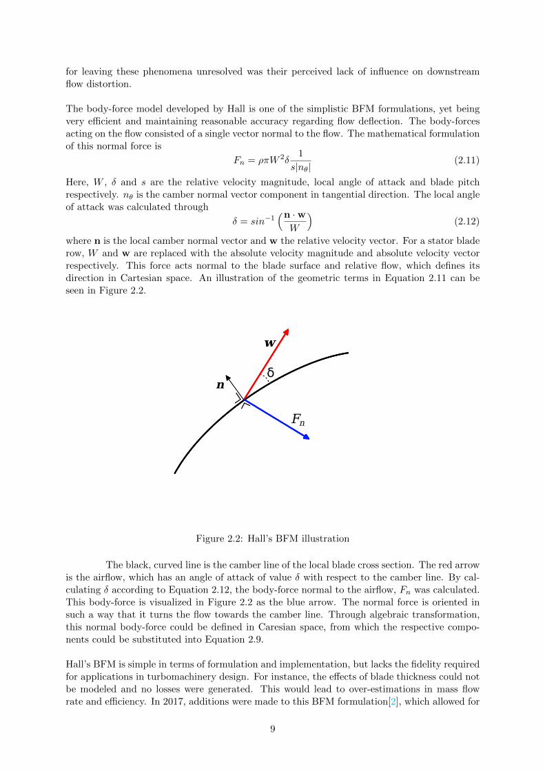
The body-force model developed by Hall is one of the simplistic BFM formulations, yet beingvery efficient and maintaining reasonable accuracy regarding flow deflection. The body-forcesacting on the flow consisted of a single vector normal to the flow. The mathematical formulationof this normal force is

Fn = ρπW 2δ1

s|nθ|(2.11)

Here, W , δ and s are the relative velocity magnitude, local angle of attack and blade pitchrespectively. nθ is the camber normal vector component in tangential direction. The local angleof attack was calculated through

δ = sin−1(n ·wW

)(2.12)

where n is the local camber normal vector and w the relative velocity vector. For a stator bladerow, W and w are replaced with the absolute velocity magnitude and absolute velocity vectorrespectively. This force acts normal to the blade surface and relative flow, which defines itsdirection in Cartesian space. An illustration of the geometric terms in Equation 2.11 can beseen in Figure 2.2.

nδ

Fn

Figure 2.2: Hall’s BFM illustration

The black, curved line is the camber line of the local blade cross section. The red arrowis the airflow, which has an angle of attack of value δ with respect to the camber line. By cal-culating δ according to Equation 2.12, the body-force normal to the airflow, Fn was calculated.This body-force is visualized in Figure 2.2 as the blue arrow. The normal force is oriented insuch a way that it turns the flow towards the camber line. Through algebraic transformation,this normal body-force could be defined in Caresian space, from which the respective compo-nents could be substituted into Equation 2.9.

Hall’s BFM is simple in terms of formulation and implementation, but lacks the fidelity requiredfor applications in turbomachinery design. For instance, the effects of blade thickness could notbe modeled and no losses were generated. This would lead to over-estimations in mass flowrate and efficiency. In 2017, additions were made to this BFM formulation[2], which allowed for

9

metal blockage and loss modeling, as well as the effects of high Mach numbers on flow turning.Throughout this report, this BFM formulation will be referred to as ‘Thollet’s BFM’, namedafter the scientist who originally implemented the blockage and loss models[2]. A 2D versionof this BFM formulation was implemented into SU2 without the loss generation and metalblockage model[6]. The normal force was formulated according to

Fn = KMachρπW2δ

1

s|nθ|(2.13)

where

KMach =

K ′ ,K ′ ≤ 3

3 ,K ′ > 3

K ′ =

1√

1−M2rel

,Mrel < 1

2

π√M2

rel−1,Mrel > 1

(2.14)

Here, Mrel is the relative, local Mach number, which in case of a stator blade row is the absoluteMach number. This factor approaches 1.0 for low Mach numbers, reaches a ceiling of 3.0 nearsonic conditions and then decreases again in supersonic flow.

The applicability of this BFM formulation and implementation was limited, as the blade shapeparameters had to be hard-coded into the solver source code. Information on the blade geometrycould therefore not be provided externally and required compilation of the solver code whenanalyzing a different blade geometry. This made the method in its current state ill-suitedfor design applications in its current state, as the computation time associated with a singlegeometry analysis would include the time required for the solver source code to compile.

2.4 Thollet’s BFM

The method described in Section 2.3 was based on Thollet’s method, but lacked the metalblockage source term and loss generation. In this section, these sub-models are elaborated upon.In blade computations, the physical presence of the blades forces the fluid to turn and acts as anobstruction in the channel. This obstruction is caused by the non-zero thickness of the blade,which results in fluid acceleration at locations of varying thickness. Apart from flow acceleration,this obstruction reduces the flow rate throughout the blade row. Due to the physical bladesnot being present in body-force modeling, these phenomena are not modeled. The governingequations for continuum flows, given in Equation 2.1, Equation 2.2 and Equation 2.3 includedthe source terms for momentum and energy present in body-force modeling, but lack any sourceterm associated with metal blockage. A geometric parameter was added to Hall’s BFM, whichwill be referred to as ‘blockage factor’, which was added by Thollet[2] and is defined as

b =s′

s(2.15)

Here, b is the metal blockage factor, s′ the local, effective pitch and s the actual blade pitch.The blade pitch is equal to

s =2πr

Nb(2.16)

where r is the local radius and Nb the number of blades in the blade row. The effective pitch,s′ is essentially the blade pitch minus the local, tangential blade thickness.This is illustrated inFigure 2.3 for a 2D cascade.

10

s′s

Figure 2.3: Definition of effective pitch and blade pitch

The ratio between the local, effective pitch and blade pitch translates to the availablethroughflow area and the area of the annulus. If the local blade thickness is high, the blockagefactor reduces, while outside of the blade row, it attains a value of 1.0. This makes the naming‘blockage factor’ to be a bit misleading, as low values translate to high flow obstruction and viceversa. The source terms implemented by Thollet to account for flow obstruction were based onthe gradient in blockage factor. If the blockage factor decreases along the flow direction, flowrate is added, which results in the flow accelerating in sections of increasing blade thickness. Ifthe blockage factor increases along the flow direction, the flow decelerates. This source termwas added to the right hand side of the steady form of Equation 2.9, resulting in the followingBFM formulation:

∂

∂xi

ρui

ρuiu1 + δi1p

ρuiu2 + δi2p

ρuiu3 + δi3p

ρuiht

=

0

F1

F2

F3

FθrΩ

−1

b

ρui

∂b∂xi

ρu1ui∂b∂xi

ρu2ui∂b∂xi

ρu3ui∂b∂xi

ρhtui∂b∂xi

(2.17)

The set of equations in Equation 2.17 can be solved using standard, time-marching techniquesused in blade computations. This formulation proved to be able to capture flow acceleration dueto blade thickness very well, but requires the distribution of the metal blockage factor through-out the bladed regions to work.

BFM formulations such as Hall’s BFM lack any form of loss generation. In physical blade rows,most losses are generated through boundary layers, shocks and endwall losses. The respectivemagnitude of these components depend on the blade geometry and flow regime. These phe-nomena can be simulated in blade computations, as the physical boundary of the blade surfaceallows for boundary layers to form and shocks to impinge upon. In body-force modeling, onlythe endwalls could generate such phenomena, but as the physical blade surface is absent, losseswould be underestimated by the BFM. In order to cope with this, an additional body-force com-ponent was added to the BFM. This component acts parallel to the flow, in opposite direction.This force component can be seen in relation to the normal body-force in Figure 2.4.

11

Fp

nδ

Fn

Figure 2.4: Illustration of the parallel body-force component

In the earliest document on body-force modeling[7], a relation between the magnitudeof the body-force component parallel to the flow and entropy generation was derived. Thisderivation can be found in Chapter 3. In order for a BFM to generate losses, a parallel body-force component was required according to this derivation. The formulation for the normal andparallel force used by Thollet were

Fn = KMachρπW2δ

1

sb|nθ|Fp = ρCfW

2 1

sb|nθ|(2.18)

where

Cf =0.0592

Re−0.2x

Rex =ρW (x− xLE)

µ(2.19)

The parallel force formulation was based on a simple, flat-plate boundary layer loss model, whereCf was used as a friction factor. The coefficient of 0.0592 was found through calibration onreference data. x− xLE is the axial distance between the leading edge and the local coordinateand µ is the fluid kinematic viscosity. In stator blade rows, the relative velocity magnitude, Wis replaced by the absolute velocity magnitude. Both the parallel and normal force magnitudeswere divided by the blockage factor, which translates to the body-force magnitude increasingnear the thicker regions of the blade. By projecting the normal and parallel body-forces into3D, Cartesian space, the body-forces can be substituted into the first right-hand side term inEquation 2.17.

12

3 Research MethodologyIn this chapter, the methodologies used to obtain the answers to the research questions arediscussed. In order to answer the research questions and solve the problems posed in Chapter 1,additions had to be made to the existing BFM in SU2 and these additions had to be verifiedthrough numerical experiments. The BFM was to be expanded to 3D, assess the effects ofblade blockage on the flow and loss generation. Formulations for these expansions were found inThollet’s BFM, which were described in Chapter 2. In order for the BFM and metal blockagemodel to function, the camber normal vector and blockage factor distribution associated withthe blade geometry had to be interpolated to the mesh nodes. This was achieved throughimplementation of a 2D interpolation algorithm into SU2. The working principles behind thismethod are explained in Section 3.1. The normal and parallel force generated by the BFM hadto be transformed to 3D, Cartesian components in order to be substituted into the body-forcesource term vector. This transformation process is outlined in Section 3.2. The additions to theexisting BFM formulation in SU2 had to be implemented in a numerically efficient manner. Theintegration of the BFM formulation into the SU2 solver structure is described in Section 3.3.In order to allow for the analysis of parameterized turbomachinery geometries using body-forcemodeling, an efficient and automated workflow process had to be set up. This would allow theuser to specify a set of design variables, defining one or multiple blade row geometries. Thegeometric parameters required for the BFM to function, as well as the mesh would have to becalculated according to this geometry prior to analysis using the BFM. This workflow processis explained in Section 3.4.

3.1 Ray-Cast Interpolation

The BFM requires the camber normal vector components and blockage factor to generate body-forces and the metal blockage source terms. Since these terms are independent of the meshgeometry and vice-versa, they had to be interpolated onto the mesh coordinates and stored oneach node. The 2D BFM implemented by M.Latour used linear interpolation for this. This waspossible, as the geometric parameters only varied in axial direction, allowing for 1D interpo-lation. For a 3D BFM, this method is insufficient, as the geometric parameters vary in 2D(inaxial and radial direction). A custom 2D interpolator was added to SU2, which made use of amathematical concept called ray-casting.

What is ray-casting theory? Ray-casting theory is based on the concept that a vector drawnfrom any point outside a region to a location inside a region intersects an odd number of timeswith the boundary of that region. This is illustrated in Figure 3.1.

13

AB

CD

X1

X2

Figure 3.1: Illustration of the ray-casting principle

Here, the black box is the boundary of the region in question, point X1 is locatedinside and X2 is located outside of the region. By drawing a line from point Y to point X1, itintersects with the boundary once, while drawing a line from Y to X2 results in two intersec-tions. According to the theory, X1 is correctly located inside the region, while X2 is not.

This principle can be used to interpolate the geometric parameters of the blade to themesh without determining separate zones in the mesh. For example, X1 and X2 are nodes inthe mesh, while points A-D form the corners of the blade and Y is the origin of the coordinatesystem. By counting the number of times a vector drawn from the origin intersects with thevirtual blade boundary, it can be determined whether the node is inside of the blade region ornot. If the node is located inside the region ABCD and geometric parameters are defined onpoints A, B, C and D, the interpolated parameters could be determined through the distance-weighted-average of the parameters at the corner points. By subdividing the blade region intoquadrilaterals, calculating the camber normal components and blockage vectors on those pointsand providing this information to the solver through an input file, the interpolation algorithmcould interpolate arbitrary blade shapes onto arbitrary meshes.

3.2 3D BFM transformation

Thollet’s BFM generates a value for the normal and parallel body-force components, accordingto Equation 2.18. In order to transform these values into a source term vector in the governingequations, these body-forces had to be transformed to a force vector in 3D Cartesian space. Inthis section, the steps taken in this transformation are outlined.

The body-force components calculated according to Thollet’s BFM were defined with respectto the local, relative flow vector and camber normal vector. This allowed for the body-forces tobe transformed to cylindrical space, of which the transition to Cartesian coordinates is trivial.The first step in the transformation process was to define the relative velocity in cylindricalcoordinates.

wcyl =

waxwθwr

(3.1)

14

By defining the rotation axis of the analysis case as a unit vector, the axial and radialcoordinates could be defined at each node.

xax =iΩ · xiΩ · iΩ

iΩ xrad = x− xax (3.2)

Here, xax is the parallel projection of the cell coordinate vector x onto the rotation axis iΩ. xrad

is the radial coordinate vector. Through normalization, these vectors could be transformed intounit vectors.

iax =xax

|xax|irad =

xrad

|xrad|iθ =

iΩ × xrad

|xrad|(3.3)

The unit vector in tangential direction, iθ was defined as the normalized cross product of therotation axis and the radial coordinate. The absolute velocity vector in Cartesian space couldnow be defined in cylindrical space.

ucyl =

uax

uθ

urad

=

uCart · iax

uCart · iθuCart · irad

(3.4)

The relative velocity vector could now be calculated through subtraction of the induced velocitydue to rotation from the tangential velocity component.

wcyl =

wax

wθ

wrad

=

uax

uθ

urad

− 0

Ω|xrad|0

(3.5)

Here, wax, wθ and wrad are the relative velocity components in axial, radial and tangentialdirection respectively. In order to translate the normal and parallel body-forces to cylindricalspace, the relative velocity parallel to the camber line was required.

wp = wcyl −wn (3.6)

wn = wcyl · n

naxnθnr

(3.7)

Here, wp and wn are the relative velocity projection vectors parallel and normal to the camberline. With the relative velocity vector parallel to the camber line, the normal body-force couldbe transformed to cylindrical space. This transformation was trivial the parallel body-force, asit acts in opposite direction to the relative flow. By adding the normal and parallel body-forcecomponents in cylindrical space, the cylindrical body-force vector was calculated.

Fcyl =

FaxFθFr

= Fn

(−cos(δ)n + sin(δ)

wp

|wp|

)− Fp

wcyl

|wcyl|(3.8)

Here, δ is the deviation angle between the relative flow and camber line, which is defined inEquation 2.12. Using the Cartesian unit vectors in cylindrical space, as defined in Equation 3.3,the cylindrical body-force vector could be defined in Cartesian space.

The resulting body-force vector could then be used as the momentum source term inEquation 2.17 and the tangential component of Equation 3.8 could be used to compute therespective energy equation source term.

15

3.3 BFM solver structure

In this section, the solver structure set up in SU2 to facilitate body-force modeling is described.The process is illustrated in Figure 3.2. The red blocks are processes which were alreadyincorporated into SU2. The blue blocks were added or modified. The process starts with thegeometry preprocessing in block 0, where SU2 defines the mesh boundaries, boundary conditionsand cell connectivity. The coordinates of the nodes are then passed to the interpolator functionin block 1.1. Here, the camber normal vectors and blockage factor values are interpolated tothe node coordinates and stored for each node.

Mesh file

BFM input file

0:Geometry

preprocessing

1.0:Solver

preprocessing

1.1:Ray-cast

interpolator

2.0:Compute body-

force source term

2.1:Compute blockage

source term

3:Recompute

flow field

Converged?

Node coordinates

Body-force parameters

No

Flow field, body-force parameters

Yes

1.2:Blockage gradient

calculator

Blockage factordistribution

Coordinates,connectivity

Flow field, body-force parameters

Figure 3.2: SU2 BFM solver structure

In order to calculate the metal blockage source term during the solution process, themetal blockage model requires the spatial gradients of the blockage factor. These are calculatedin block 1.2, using the finite-difference-method used by the solver to calculate the gradients inflow variables, but using the interpolated blockage factor values as input.

After passing through blocks 1.1 and 1.2, all geometric parameters required for theBFM to calculate the body-forces were calculated and stored on each node. The actual solvingprocess could initialize after block 1.0, where the body-force and blockage source terms arecalculated and added to the governing equations. The flow field is recomputed and this pro-cess is repeated until convergence. The flow variables, body-forces and interpolated geometricparameters are included in the solver output for postprocessing.

3.4 Automated Workflow for BFM Computations

In order to prepare the BFM for design optimization in future studies, an automated workflowtranslating a set of design variables to SU2 input was required. In this section, the automatedworkflow process developed for this purpose is outlined.Due to the complex shape of modern turbomachinery blades, a high number of design variablesis often used for blade optimization. However, at a first-level conceptual stage, this is oftenreduced to a set of duty coefficients, of namely the flow coefficient(φ), work coefficient(ψ) anddegree of reaction(R∗). These three duty coefficients allow for the definition of the blade inletand outlet angles and therefore allow for the creation of a simplified geometry with a low number

16

of variables. The method put in place allowed for expansion to higher variable counts if desired.

The goal of this workflow process was to take these high-level design variables and translatethem to a mesh and the inputs required for the BFM. This would result in a streamlined designprocess. Figure 3.3.

Duty coefficientsWorking fluid

Boundary conditionsBlade thickness distribution Mesh parameters

1.1:Meangen

Blade metal anglesAnnulus shape

1.3:GMesh/ICEM

SU2/CGNS mesh

1.4:SU2 PERIO

1.2:Parablade

Loop over blade rows

Blade row anglesSection coordinates

Axisymmetric, periodic mesh

Camber normalsBlockage factors

Writing BFMparameters to file

BFM input file

Figure 3.3: BFM preprocessing workflow diagram

The BFM preprocessing starts with the definition of design variables, working fluid pa-rameters, boundary conditions, blade thickness distribution and mesh parameters. The processinitializes with a progam called Meangen. Meangen is able to convert high-level design variablesinto a simplified geometry, which includes the blade metal angles and meridional blade shape fora specified number of stages. Meangen can be used for axial, radial and mixed-flow machines,but in this workflow, only axial machines are considered. The BFM requires a distribution ofcamber normal and metal blockage data, for which a more detailed blade geometry is required.This detailed geometry is generated through a program called Parablade.

Parablade is a Python-based code developed within the Propulsion and Power groupat TU Delft. It is used to generate detailed blade shapes which can be used to create meshesfor turbomachinery analyses. Parablade allows the user to specify an almost arbitrary numberof design variables, making it a powerful tool in shape optimization of turbomachinery bladerows. Additionally, the code is able to generate geometry sensitivity distributions based on thespecified design variables, which allows for the computation of the design sensitivities in adjointoptimization. The Parablade code was modified to allow for BFM preprocessing as well. Here,the axial and radial distribution of camber normal vectors and blockage factor are calculated,

17

which can be used in SU2 for BFM computation.

After Meangen returns the crude blade geometry, Parablade is initialized for eachconsecutive blade row to produce the distribution of camber normals and blockage factors. Itstores this information in a file which can be read by the 2D interpolation algorithm in SU2.The input parameters of Parablade include the blade metal angles and annulus shape fromMeangen output and the blade thickness distribution defined by the user. Meangen also usesblade thickness parameters as input, but these could not be translated to the blade thicknessparameterization used in Parablade, which is why these had to be defined during initialization.The blade parameterization in Parablade is based on Bezier-curves. The blade camber line isdefined at several sections along the blade span. The blade surface is generated by a curve offsetby half the local thickness, normal to the camber line. This camber normal vector distributionwas used as input for the BFM in SU2. The blockage factor distribution was calculated throughinterpolation of the blade upper and lower surface and calculating the effective pitch trend inaxial direction. By dividing these by the blade pitch, the blockage factor distribution could bedefined. After looping through all the blade rows, the camber normal and blockage distributionof all blade rows were merged into a single input file which could be read by SU2.

With the annulus shape defined through Meangen, the flow domain could be discretizedinto a mesh. The BFM meshing procedure was relatively simple, as the detailed blade shapewas not required. The only inputs required were the annulus shape produced in step 1.1 byMeangen and mesh size parameters provided by the user. Two variations in mesh generationwere incorporated into the process. The program used for unstructured meshing was GMesh.GMesh is a meshing software which can be controlled through Python as a module to produceunstructured meshes for relatively simple geometries. The meshing parameters the user canprovide are the number of cells in axial direction for each blade row, mesh density reductionfactors for the inlet and outlet section of the mesh and the number of cells in pitch-wise direc-tion. The structured meshing option was ANSYS ICEM. Here, the only mesh parameter whichwas used for this research project was the axial node count. Additional refinement was appliednear the leading and trailing edges of the blade rows, while using exponential cell size relationswere used in the far field.

Structured and unstructured meshes have respective benefits and drawbacks with respect tobody-force modeling. The unstructured mesh is fully independent of the meridional bladeshape, allowing for the mesh to be reusable given that the annulus shape remains constant. Adrawback is that the solver process is less efficient and the total node count is not optimizedfor the geometry. Using a structured mesh allows the user to reduce the total number of nodes,as the cell aspect ratio allows for axial refinement, while keeping the number of cells in radialdirection constant. Additionally, the interpolation onto the mesh nodes results in more smoothdistributions and a better approximation of the gradient in blockage factor. The meshes gen-erated by ICEM or GMesh can be read by SU2, but are not suitable for axisymmetric BFManalysis yet. SU2 PERIO is used to transform the mesh produced by GMesh or ICEM into aperiodic mesh.

Upon finishing this research project, the unstructured GMesh procedure was fully automated,while that involving ICEM still required manual adjustment. In the near future, also thisprocedure is expected to be automated. This preprocessing workflow proved to be a valuabletool in performing BFM analyses as it was easy to use and very efficient. Even for multiplestages, the entire process takes less than one minute when defining an axisymmetric case. Inthe future, this tool could be expanded to include full-annulus meshing and design capabilitiesthrough adjoint-solving.

18

4 BFM VerificationBefore comparing the performance of the BFM to the results of high-fidelity blade computa-tions, its correct implementation had to be verified. In this section, the methods used to verifythe implementation of the body-force model are described, in particular the metal blockage andparallel force additions to the exiting BFM formulation. The verification processes were carriedout through result comparison of theoretical trends or blade computation results. In Section 4.1,the verification methodology of the parallel force addition is given, while that of the blockagesource term addition and 2D interpolation can be found in Section 4.2.

4.1 Verification of Parallel Force Implementation

The parallel force addition to the BFM allows for entropy generation in the BFM simulation.This capability had to be verified to ensure its proper functionality and implementation. Theexperiment used for verifying the parallel force functionality was to compare the BFM outputof a flat plate stator geometry to the theoretical solution.

The governing equations used for this simulation were the steady Euler equations, with theworking fluid being air. In order to verify the parallel force implementation, the simulationentropy and pressure gradient results are compared to the theoretical trends they would havefor a flat plate case. During the upcoming derivations, the following set of assumptions wereapplied.

• Incompressible flow: Free-stream Mach number is below 0.3, constant density, constantaxial velocity.

• Perfect gas: Gas constantR = 287.1 J kg−1 K−1, specific enthalpy cp = 1004.7 J kg−1 K−1,specific heat ratio γ = 1.4

• Constant kinematic viscosity: µ = 1.716× 10−5 kg m−1 s−2

• Adiabatic flow: No heat transfer between the geometry and the flow or the flow andthe endwalls.

• Parallel force only: Stator angle is zero degrees, no flow deflection in tangential direc-tion, camber normal components in axial and radial direction are equal to zero, nθ = 1.0.

• Inviscid flow: No turbulent source terms in the governing equations. The only viscousterms are introduced through the parallel force.

• Axial, 1D, steady flow: No unsteady terms in the governing equations, flow only inaxial direction.

• No metal blockage: Blockage factor set to 1.0, blockage gradient throughout the flowfield is zero.

Due to the inviscid assumption, the Euler equations were used for the derivation. The Eulermomentum equation in x-direction is equal to

∂(ρu2x)

∂x+∂(ρuyux)

∂x+∂(ρuzux)

∂x+∂p

∂x= Fx (4.1)

Here, Fx is introduced by the BFM. Due to the flow being axial, all velocity components in yand z-direction are set to zero. Also, due to the flow being assumed incompressible, the density

19

was assumed constant. Finally, the combination of the flow being incompressible, the crosssection being constant and the case being steady, the axial velocity component is constant.This simplifies the axial momentum equation to

d(ρu2x)

dx+dp

dx= Fx →

dp

dx= Fx (4.2)

Since only the parallel force acts on the flow in opposite direction to the velocity, the body-forcecan be rewritten as

Fx = −Fp (4.3)

This would mean that the pressure gradient in axial direction would match the negative parallelforce trend. If significant differences in the shape of the trends were to be found, it would meanthat either the set of stated assumptions didn’t apply or the parallel force implementation wasfaulty.

The parallel force was implemented to model entropy generation. The following derivations werecarried out in order to predict the entropy change throughout the blade row. For the entropychange across any blade row, the following equation is considered.

Tds = dH − vdp = cpdT −RT

pdp (4.4)

Dividing by dx to get entropy gradient in axial direction:

Tds

dx= cp

dT

dx− RT

p

dp

dx(4.5)

The pressure gradient was already computed according to Equation 4.2. To get the temperaturegradient, the body-force source term in the energy equation needs to be considered. The sourceterm in the energy equation for the BFM is equal to rΩFθ. In case of the flat plate stator, thisterm is equal to zero, resulting in the temperature gradient to be zero.

∂(ρuxht)

∂x+∂(ρuyht)

∂y+∂(ρuzht)

∂z= ΩrFθ (4.6)

ρuxdhtdx

= 0→ ρuxd (cpT )

dx= 0 (4.7)

ρuxcpdT

dx+ρux2

d(u2x)

dx= 0 (4.8)

Due to the flow being incompressible with a constant flow area, the velocity gradient is zero.This simplifies the temperature gradient to

ρuxcpdT

dx= 0→ dT

dx= 0 (4.9)

Since the pressure gradient is unaffected by the change in energy source term, the entropygradient equation becomes

Tds

dx= −1

ρ

dp

dx=

1

ρFp (4.10)

By comparing the pressure and entropy gradient to the parallel force trend across the flow do-main, the correct implementation of the parallel force can be verified. If the entropy gradientand negative pressure gradient equal the parallel force, the BFM source term was implementedcorrectly.

20

The flow simulation domain used for the verification of these equations can be seen in Figure 4.1.The mesh was set up to be a structured mesh, generated in ICEM. The body-forces acted in thered region, where the mesh was refined to ensure grid convergence. The mesh was also refinednear the leading and trailing edges of the bladed region, which ensured a more smooth solution.The mesh was set one cell wide in pitch-wise direction, as the BFM theoretically doesn’t requiremesh refinement in that direction for axisymmetric simulations. Whether this is true was testedin a different experiment.

Figure 4.1: axial-radial slice of parallel force verification domain

The simulation used the following set of boundary conditions, as can be seen in Ta-ble 4.1. The total-to-static pressure ratio between the domain inlet and outlet was set to 1.04,which is lower than the sonic pressure ratio for air, which is about 1.8. With this pressure ratio,no compressible flow within the domain was expected.

Table 4.1: Parallel force verification boundary conditions

Boundary Boundary conditions

Inlet pt = 105 325 Pa, Tt = 288.7 K

Outlet ps = 101 325 Pa

Hub, Shroud slip-wall

After convergence of the solution, the values for entropy generation and static pressure trendswere extracted from the solution flow field through averaging over the radial-tangential slice. Theentropy and pressure gradients were obtained through finite-difference. As no significant radialand tangential flow components were expected, the parallel force magnitude could be assumedequal to the negative body-force magnitude in axial direction. With these data, Equation 4.2and Equation 4.10 could be visualized, through which the parallel force implementation couldbe verified.

4.2 Metal Blockage Model Verification

The main goal of the metal blockage term implementation was to model the flow obstructionby the blades. Before analyzing the performance of the BFM, the functionality of the metalblockage implementation had to be validated. This was done through comparison of bladecomputation and BFM flow simulation data of a symmetric, prismatic stator geometry with anonzero thickness distribution. This resulted in a blockage factor distribution within the bladesection with values lower than 1 and a nonzero blockage gradient distribution. Especially by

21

comparing the mass flux trends in axial direction, the flow obstruction capability of the metalblockage model could be assessed. In Figure 4.2, the cross section of the blade can be seen. Thethickness distribution was chosen to be parabolic for simplicity and also to test the accuracy ofthe interpolator, as the blockage factor distribution can be expressed analytically.

0.0 0.2 0.4 0.6 0.8 1.0xc

−0.4

−0.3

−0.2

−0.1

0.0

0.1

0.2

0.3

0.4

t c

Blade contour

Figure 4.2: Prismatic cross section used for metal blockage verification

The validation run was performed in 3D through an axisymmetric turbomachinery simulation.In Table 4.2, the dimensions of the blade geometry can be found. Here, tmax is the maximumthickness of the blade, c the axial chord and Nblade the number of blades in the blade row. Forsimplicity, no hub or tip gaps were applied.

Table 4.2: Geometric parameters of blade geometry used for blockage verification

Parameter Dimension

rhub 0.25 m

rshroud 0.325 m

tmax 5 mm

c 0.05 m

Nblade 30

The blockage factor distribution could be expressed analytically, due to the cross section beingparabolic. For a parabolic cross section with its maximum thickness in the middle, the thicknessas a function of axial coordinate is equal to

t(x) = 4tmax

cx− 4

tmax

c2x2 (4.11)

The blockage factor is equal to the ratio between the local channel width and the blade pitch.In this case, the channel width is equal to the pitch minus the blade thickness. The theoreticalblockage factor distribution could therefore be expressed as

b(x, r) =

2πrNblade

− 4(tmaxc x− tmax

c2x2)

2πrNblade

(4.12)

22

This expression was used to verify the implementation of the 2D interpolation algorithm, bycomparing the interpolator output for the blockage factor to Equation 4.12. By plotting thedeviation and calculating the root-mean-square(RMS) error of the interpolated blockage field,the accuracy of the interpolator could be determined. If the error was found to be below anacceptable limit, the interpolation algorithm was deemed to be implemented correctly and func-tioning properly.

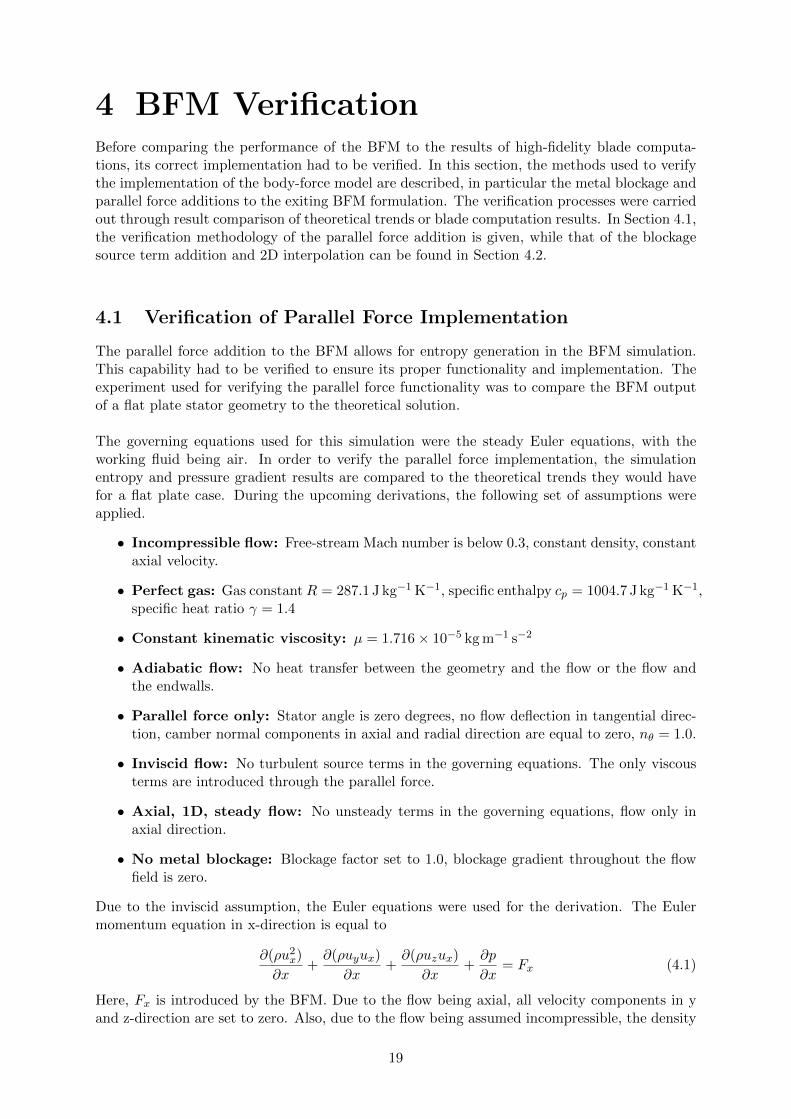
In order to quantify the accuracy of the metal blockage model, the results obtained throughblade computation and body-force modeling had to be compared. This was achieved throughsetting up a blade computation and BFM flow domain of the same blade geometry with similarboundary conditions. For both simulations, an Euler solver scheme was used. In an Eulersimulation, no boundary layers are resolved. Therefore, the only flow obstruction in the bladecomputation would be due to metal blockage and no boundary layer blockage. In the BFMsimulation, the parallel force was disabled. This way, the only source terms acting on the flowwould be introduced by the metal blockage model. In Figure 4.3, the mesh can be seen whichwas used to obtain the results of the blade computation of the stator geometry. In Figure 4.4and Figure 4.5, 2D slices of the blade computation domain can be seen, in which the fluidboundaries are identified.

Figure 4.3: 3D mesh used for the blockage verification blade computation

23

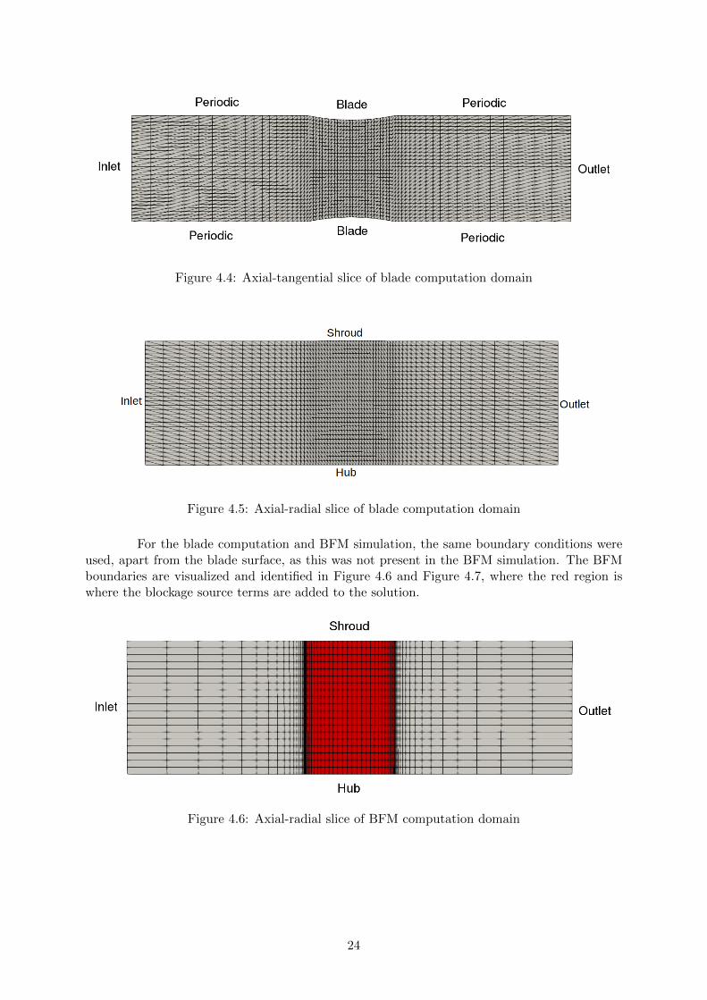
Figure 4.4: Axial-tangential slice of blade computation domain

Figure 4.5: Axial-radial slice of blade computation domain

For the blade computation and BFM simulation, the same boundary conditions wereused, apart from the blade surface, as this was not present in the BFM simulation. The BFMboundaries are visualized and identified in Figure 4.6 and Figure 4.7, where the red region iswhere the blockage source terms are added to the solution.

Figure 4.6: Axial-radial slice of BFM computation domain

24

Figure 4.7: Axial-tangential slice of BFM computation domain at mid-span

In Table 4.3, the boundary conditions for the boundary markers in Figure 4.4, Fig-ure 4.5, Figure 4.6 and Figure 4.7 are listed. The working fluid in these simulations was setto be standard air, with the same properties as listed in the assumptions for the parallel forcederivations in Section 4.1.

Table 4.3: Boundary conditions used for the blockage verification simulations


Inlet pt = 105 325 Pa, Tt = 288.7 K

Outlet ps = 101 325 Pa

Hub and shroud slip-wall

Blade surface slip-wall

By comparing the averaged pressure and axial mass flux trends of the BFM and bladecomputation results, the accuracy of the blockage source term model could be found. This wasdone through plotting the error along axial direction to see where the deviation was the highestand by computing the RMS. If the RMS was found to be below an acceptable limit, the blockagesource term model was considered to work correctly.

25

5 BFM Case StudyAfter verifying the proper implementation of the BFM parallel force and blockage implementa-tion, it was possible to compare BFM data to that of blade computations of actual turboma-chinery geometries. The case chosen for this purpose was the Aachen turbine case. This is anaxial, low speed turbine geometry with one rotor row in between two stator rows. The hub andshroud surfaces were defined as free slip walls and no tip gap was present in the rotor row. Thismade the case suitable for validation purposes, as annulus boundary layers are not modeled bythe BFM and no tip gap modifications were implemented. By comparing the flow data from theAachen turbine blade computation and those resulting from the BFM, the accuracy of the BFMcould be quantified. In order to quantify the computational efficiency, the total computationtimes required for convergence were compared between the methods. This was done for severalvariations in mesh density for the BFM in order to visualize the trade-off between accuracy andcomputational efficiency.

5.1 Aachen Turbine Blade Computation Setup

The blade rows of the Aachen turbine consisted of prismatic blades with no tip or hub gap,with 41 blades in each row and a rotor rotation speed of 3500 rpm.The flow domain used for theblade computation can be seen in Figure 5.1. In Figure 5.2 and Figure 5.3, the cross sectionsof the Aachen turbine stator and rotor can bee seen respectively.

Figure 5.1: Aachen turbine flow domain

26

0.00 0.01 0.03 0.04x axis

−0.05

−0.04

−0.03

−0.02

−0.01

0.00y ax

is

Figure 5.2: Aachen stator cross section

0.06 0.07 0.09 0.10 0.12x axis

−0.03

−0.02

−0.01

0.00

0.01

0.02

0.03

0.04

y ax

is

Figure 5.3: Aachen rotor cross section

The blade computation performed on this geometry was a RANS computation using a κ − ω-SST turbulence scheme with the boundary conditions listed in Table 5.1. The total number ofcells in the mesh was in the order of 1.8× 106.

Table 5.1: Aachen blade computation boundary conditions


Inlet pt = 155 000 Pa, Tt = 308 K

Outlet ps = 99 614.9 Pa

Blade surfaces no-slip wall

Hub and shroud symmetry

Table 5.2: Aachen blade computation direct solver settings

Setting Type Value(s)

Turbulence model κ− ω-SST

Fluid model Ideal gas R = 287.058 J kg−1 K−1

γ = 1.4

Viscosity model Sutherland CS = 110.4

µref = 1.716× 10−5 kg m−1 s−2

Tref = 273.15 K

Conductivity model Constant Prandtl number CKT = 0.0257

Spatial gradient model Weighted least squares

Linear solver FGMRES Error=1e− 4, iterations=15

Flow numerical method JST Sensor coefficients=(0.3, 0.18),Relaxation factor=0.75

Turbulent numericalmethod

Scalar upwind Relaxation factor=0.95

27

5.2 BFM Computation Setup

One of the advantages of using a BFM compared to a blade computation is the relatively coarsemesh associated with BFM computations. By performing a mesh study on the BFM mesh usedfor the Aachen turbine case study, it was possible to find the level of mesh refinement requiredto reproduce the results from the blade computation.

The inlet, outlet, hub and shroud boundary conditions of the blade computation were carriedover to the BFM simulation in order to ensure case similarity. The flow solver conducting theBFM simulation was the Euler solver. The reason why this solver was used instead of the RANSsolver applied in the blade computation was the lack of viscous phenomena to be resolved. Theannulus walls of the domain were identified as slip-walls, along which no boundary layers form.Therefore, the only relevant viscous phenomenon occurring in the flow would be the boundarylayer on the blade surface. This phenomena is modeled by the parallel force model in the BFM,which therefore made the necessity for a viscous flow solver obsolete.

The two mesh parameters used in the mesh study were the number of nodes in axial directionper blade section and the mesh wedge angle. Both are illustrated in Figure 5.4 and Figure 5.5respectively.

Figure 5.4: Axial node count definition

In Figure 5.4, the first mesh study parameter is illustrated. The red regions are the meridionalprojections of the turbine blades. By varying the axial node count (Nx) in those regions, theoverall mesh density was adjusted. A high value for Nx therefore resulted in a more refinedmesh, while the opposite was true for low values of Nx. In this part of the mesh study, Nx

was varied between 10 and 60 nodes for all three blade rows. One extra run with a value of100 for Nx was performed in order to have a reference trend for (assumed) grid convergence.The convergence criterion for both the BFM and blade computation results was set to a densityresidual value of 10−16. By comparing the computation times of the blade computation andBFM simulations, the relative computational efficiency of the BFM was determined.

The mesh wedge angle parameter was varied to verify the independence of the BFM on thedomain pitch. In order to verify this property, solutions of BFM simulations using varyingcell counts in pitch-wise direction were compared. The mesh parameter used for this study isillustrated in Figure 5.5.

28

Figure 5.5: Tangential node count definition

Here, Nθ is the node count in tangential direction. By varying the pitch angle and applying onecell per degree of pitch angle, the number of cells along the arrows was varied. By performingBFM computations on meshes with varying wedge angle parameters, while maintaining a con-stant value for Nx, it was possible to verify the BFM independence on pitch-wise node count.This would be the case if the averaged result trends of the different wedge angles overlap. Ifthis would be the case, it would mean that axisymmetric BFM simulations could be performedon meshes of one cell wide, which substantially increases computational efficiency due to thelimited cell count in the mesh. The tangential node count was varied between Nθ = 1 andNθ = 4 with a constant Nx = 20.

29

6 ResultsIn this chapter, the results from the various verification steps and mesh study are given. Thevarious methodologies in Chapter 3 were set up to provide insight into the correct functionalityof the BFM. The results of these tests inspire confidence in the workings of the new additionsto the BFM if they comply to reference data. Once verified, the BFM was to be appliedin an actual turbomachinery analysis case, where the BFM results were compared to bladecomputation data in order to determine the accuracy and computational efficiency with respectto the blade computation. The results regarding the parallel force addition can be found inSection 6.1. The results of the blockage factor verification experiment and interpolator qualityare in the subsequent Section 6.2. Finally, the results regarding the Aachen turbine mesh studycan be found in Section 6.3.

6.1 Verification of Parallel Force Implementation

In this section, the results of the parallel force verification are presented. The numerical setupand boundary conditions can be found in Section 4.1. With a constant CFL number of 8.0, thesimulation converged steadily. The density residual convergence trend can be seen in Figure 6.1.The trend somewhat fluctuated initially while descending, but after about 3000 iterations, thischanged to a nearly linear descend.

0 1000 2000 3000 4000 5000 6000Iteration[-]

−16

−14

−12

−10

−8

−6

Resid

ual v

alue

[-]

ρ residual

Figure 6.1: Density residual convergence trend

After convergence, the flow data was processed. In order to verify the parallel force implemen-tation through Equation 4.2 and Equation 4.10, the pressure and entropy gradients had to beobtained. This was achieved through numerical differentiation on the area-averaged pressureand entropy trends. In Figure 6.2, the comparison between the entropy trend and parallel forcecan be seen. The trends overlap for the most part, apart from near the leading and trailingedge of the blade section. This fluctuation is probably caused by the high gradient in body-forcemagnitude. In the cells right outside the body-force zone, no source terms are added to thegoverning equations, while in the adjacent cells, this term is nonzero. This behaviour was alsofound in Latour’s work[6]. Apart from the fluctuations near the leading and trailing edge, theentropy gradient seemed to have been calculated correctly by the BFM, as the trends overlapcompletely.

30

−0.10 −0.05 0.00 0.05 0.10 0.15x[m]

0

250

500

750

1000

1250

1500

Tds dx[Jk

g−1 m

−1]

Parallel force vs entropy gradient

Tdsdx1ρFp

Figure 6.2: Comparison between entropy gradient and parallel force

In Figure 6.3, the comparison between the parallel force and pressure gradient can be seen.Similar to Figure 6.2, some fluctuation of the pressure gradient can be seen near the bladeedges. In this case, the two trends are offset, although the behaviour seems to agree.

−0.10 −0.05 0.00 0.05 0.10 0.15x[m]

−2000

−1500

−1000

−500

0

dp dx[kgm

−2s−

2 ]

Parallel force vs pressure gradientdpdx

−Fp

Figure 6.3: Comparison between pressure gradient and parallel force

The reason for the offset had to do with the flow not being fully incompressible. The averageMach number was about 0.24, which is generally considered to be on the edge of the compressibleregime. This caused the gradient in kinetic energy to be significant. Therefore, the momentumterm on the left hand side of Equation 4.2 should be taken into account. When subtractingthe gradient in kinetic energy from the parallel force, the trends overlap completely, as can beseen in Figure 6.4. The results of the flat plate run with the parallel force term implementedresulted in Equation 4.2 and Equation 4.10 to be satisfied, therefore verifying its functionality.

31

−0.10 −0.05 0.00 0.05 0.10 0.15x[m]

−2000

−1500

−1000

−500

0

dp dx[kgm

−2s−

2 ]

Parallel force vs pressure gradientdpdx

−Fp−Fp− d(ρu2

x)dx

Figure 6.4: Comparison between pressure gradient and parallel force with inclusion of kineticenergy gradient

6.2 Verification of Metal Blockage Model Implementation

The main goal of the blockage factor verification was to verify the BFM’s ability to model flowobstructions. If the model was to operate accordingly, the flow should accelerate in the bladeregion, reaching a maximum velocity at the height of the thickest portion of the blade. As wassaid in the experiments description, the parallel force was disabled for this run, as friction wasnot considered in the blade computation.

After interpolating the body-force parameters, the accuracy of the 2D interpolation algorithmcould be determined. In Figure 6.5, the blockage factor distribution along the axial and radialaxis throughout the flow field can be seen, alongside the distribution according to Equation 4.12.

Figure 6.5: Comparison between interpolated and analytical blockage factor distribution

32

From a qualitative point of view, these distributions seem nearly identical. In order to obtaina quantitative measure for the level of accuracy of the interpolator, the deviation between thetheoretical and interpolated blockage factor was calculated and visualized. In Figure 6.6, thedeviation between the blockage factor field as it was interpolated and the theoretical blockagefactor distribution is displayed.

Figure 6.6: Comparison between interpolated and analytical blockage factor distribution

The deviation fluctuated between -0.15% and 0.15% throughout the blade region. The RMSerror within the bladed region was calculated to be 0.041%, indicating that the error fluctua-tion was relatively high compared to the average value. There were some differences expectedbetween the theoretical and interpolated distributions, as the mesh was relatively coarse (20nodes in axial direction within the bladed region) and the mesh used a different axial node dis-tribution (biexponential) compared the blade shape provided as input(uniform). Despite thesedifferences, the interpolator was able to approach the theoretical solution accurately. The RMSdifference of 0.041% was deemed low enough to continue using the method for further analyses.

After completion of the BFM and blade computation simulations, the results were analyzed andcompared. Both the BFM and blade computation converged to their respective convergencetargets set to a density residual of 10−16. In Figure 6.7 and Figure 6.8, the Mach numberdistribution of the BFM and blade computation can be seen respectively. Both figures show thecontour of the Mach number on the blade-to-blade plane at mid-span.

Figure 6.7: Mach number distribution in BFM results (radius=0.2875 m)

33

Figure 6.8: Mach number distribution in the blade computation results(radius=0.2875 m)

When looking at Figure 6.8, the flow-through area contracts and expands in the blade row, re-sulting in respective flow acceleration and deceleration, especially near the blade surface. Sincethe BFM replaces the blade by a volumetric force field, the effective presence of the blade rowis constant in tangential direction. This, combined with the flow conditions being uniform uponentering the domain causes the flow to be uniform in tangential direction.

In order to check whether the metal blockage model performed correctly, the area averagedMach number, mass flux and pressure trends of the BFM and blade along the rotation axiscomputation were compared. In Figure 6.9, Figure 6.10 and Figure 6.11 the respective averagedMach number, mass flux and normalized static pressure trends are displayed. The black, dottedline represents an error margin of 1% with respect to the blade computation results.

−0.10 −0.05 0.00 0.05 0.10 0.15Axial coordina e[m]

0.235

0.240

0.245

0.250

0.255

0.260

M[−

]

Mach number comparisonBlade compu a ion+-1%BFM

Figure 6.9: Mach number comparison between blade computation and BFM

34


98

100

102

104

106

108ρu

x[kgm

−2s−

1 ]Mass flux comparison

Blade compu a ion+-1%BFM

Figure 6.10: Mass flux comparison between blade computation and BFM


0.945

0.950

0.955

0.960

0.965

0.970

p s p t,in

Pressure comparisonBlade compu a ion+-1%BFM

Figure 6.11: Normalized static pressure comparison between blade computation and BFM

For all three trends, the averaged BFM and blade computation results are in good agreement.The Mach number increases in the converging section of the blade and then decreases in thediverging section, returning to the same value the flow had upon entering the blade row. InFigure 6.12, the deviation between the mass flux trends of the BFM and blade computationresults can be seen, alongside 1% margins shown, indicated by the black, dotted lines.

35

−0.10 −0.05 0.00 0.05 0.10 0.15Axial coordinate[m]

−1.00

−0.75

−0.50

−0.25

0.00

0.25

0.50

0.75

1.00

Error[%

]

Mass flux deviationError+-1%

Figure 6.12: Deviation between BFM mass flux and blade computation mass flux trends

In the far field regions, the BFM overestimated mass flux by about 0.12%, while in the bladedregion, this difference increased to 0.35%. Overall, the RMS error of the mass flux was calculatedto be 0.18%. This deviation is about an order of magnitude higher than the interpolation RMSerror, so the error was likely not caused by the inaccuracy intruduced by the interpolationmethod.

6.3 Aachen Turbine Case Study Results

In this section, the results of the Aachen turbine mesh study are presented. A comparison wasmade between the blade computation and BFM results, where the mesh density and numberof cells in axial and tangential direction were varied respectively. The accuracy of the BFMwas measured through axial trend comparison of several relevant flow variables. These weremass-flux-averaged over the radial-tangential plane in order to produce clear trends. Throughcomputation of the deviation between the BFM and blade computation results, it was possibleto determine the magnitude and location of inaccuracies of the BFM.

6.3.1 Results as a Function of Axial Node Density

The BFM simulations converged successfully to their respective convergence target. In Fig-ure 6.13, the convergence trends of the different meshes can be seen. All BFM simulations wereperformed using a single processor, with a constant CFL number of 8.0. The mesh with thehighest density, having 100 nodes in axial direction per blade row, took about 220 minutes toconverge, while that of the least dense mesh took less than 30 seconds. The blade computa-tion took about 52 hours wall clock time on 20 processors to converge to the same level. Thisdemonstrates the high computational efficiency of the BFM. This means that the BFM overallconverged 3 orders of magnitude faster than the blade computation.

36

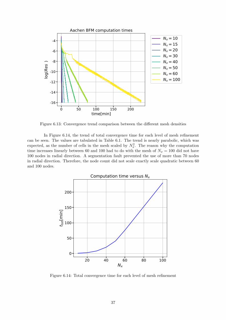
0 50 100 150 200time[min]

-16

-14

-12

-10

-8

-6

-4log(Re

s ρ)

Aachen BFM computation timesNx=10Nx=15Nx=20Nx=30Nx=40Nx=50Nx=60Nx=100

Figure 6.13: Convergence trend comparison between the different mesh densities

In Figure 6.14, the trend of total convergence time for each level of mesh refinementcan be seen. The values are tabulated in Table 6.1. The trend is nearly parabolic, which wasexpected, as the number of cells in the mesh scaled by N2

x . The reason why the computationtime increases linearly between 60 and 100 had to do with the mesh of Nx = 100 did not have100 nodes in radial direction. A segmentation fault prevented the use of more than 70 nodesin radial direction. Therefore, the node count did not scale exactly scale quadratic between 60and 100 nodes.

20 40 60 80 100Nx

0

50

100

150

200

t tot[m

in]

Computation time versus Nx

Figure 6.14: Total convergence time for each level of mesh refinement

37

Table 6.1: Tabulated total computation time for each level of mesh refinement

Nx 10 15 20 30 40 50 60 100

Time[min, sec] 0, 26 1, 19 2, 50 8, 16 19, 58 41, 8 76, 6 230, 11

The relatively high computational efficiency of the BFM with respect to the blade computationwas considered to be a significant benefit of using body-force modeling in design applications.However, for such applications, relative accuracy is equally as important. In Figure 6.15, themass flow averaged trends of the normalized static pressure according to the BFM and bladecomputation simulations can be seen. When globally comparing the BFM and blade compu-tation results, the BFM appears to agree very well to the blade computation results, alwaysremaining within 5% error margin.

-0.05 0.00 0.05 0.10 0.15 0.20x[m]

0.60

0.70

0.80

0.90

1.00

1.10

p p t,in

Mass flow averaged ressure lotBlade com utationBody− force,Nx=10Body− force,Nx=15Body− force,Nx=20Body− force,Nx=30Body− force,Nx=40Body− force,Nx=50Body− force,Nx=60Body− force,Nx=100+- 10%+- 5%

Figure 6.15: Comparison of nomalized static pressure trends

In Figure 6.16, the exact percentile deviation of the BFM static pressure trends can beseen. The BFM overestimated the static pressure by a maximum of 3% near the trailing edgeof the rotor, after which it underestimated it in the second stator row.

38

-0.05 0.00 0.05 0.10 0.15 0.20x[m]

-2.00

-1.00

0.00

1.00

2.00

3.00ε p

s[%]

Static pressure deviationNx=10Nx=15Nx=20Nx=30Nx=40Nx=50Nx=60Nx=100

Figure 6.16: Static pressure deviation

The stagnation pressure trend behaved similarly to the static pressure trend, whichcan be seen in Figure 6.17. There does seem to be some difference between the stagnationpressure trends within the rotor row. Whereas the trend of the blade computation immediatelydecreased with a near constant gradient, the BFM initially shows a more gradual decrease andends up at a slightly lower stagnation pressure value compared to that of the blade computation.The stagnation pressure deviation with respect to the blade computation results is shown inFigure 6.18. Due to the parallel force, a total pressure drop across the two stator rows can beseen and the outlet total pressure is approximated within 1%. The highest deviation is seenthroughout the rotor, where the deviation peaks at around 5.5%, after which the deviationremains within 1%.

-0.05 0.00 0.05 0.10 0.15 0.20x[m]

0.75

0.80

0.85

0.90

0.95

1.00

1.05

1.10

p t p t,0

Mass flow averaged stagnation ressure lotBlade com utationBody− force,Nx=10Body− force,Nx=15Body− force,Nx=20Body− force,Nx=30Body− force,Nx=40Body− force,Nx=50Body− force,Nx=60Body− force,Nx=100+- 10%+- 5%

Figure 6.17: Comparison of nomalized total pressure trends

39

-0.05 0.00 0.05 0.10 0.15 0.20x[m]

-2.00

-1.00

0.00

1.00

2.00

3.00

4.00

5.00

6.00ε p

t[%]

Stagnation pressure deviationNx=10Nx=15Nx=20Nx=30Nx=40Nx=50Nx=60Nx=100

Figure 6.18: Stagnation pressure deviation

The stagnation temperature comparison can be seen in Figure 6.19. The BFM correctlyshows no stagnation temperature drop in the stator rows, as no work is extracted in thoseregions. Over the rotor row, the stagnation temperature drops. There seems to be somewhatof a difference between the shape of the trends there, but the overall stagnation temperaturedrop over the rotor row is approximated well within 1%.

-0.05 0.00 0.05 0.10 0.15 0.20x[m]

0.85

0.90

0.95

1.00

1.05

1.10

T t T t,0

Mass flow ave aged stagnation tempe atu e plotBlade computationBody− force,Nx =10Body− force,Nx =15Body− force,Nx =20Body− force,Nx =30Body− force,Nx =40Body− force,Nx =50Body− force,Nx =60Body− force,Nx =100+- 10%+- 5%

Figure 6.19: Comparison of nomalized total temperature trends

The stagnation temperature trend was reproduced more accurately by the BFM com-pared to the stagnation pressure. In Figure 6.18, the stagnation temperature deviation trendscan be seen. The shape of the deviation is similar to the stagnation pressure deviation trend inFigure 6.18, but it peaks at around 1.5% instead of 5.5%. When looking at the outlet stagnationpressure deviation, it underestimated the extracted work within 0.5%.

40

-0.05 0.00 0.05 0.10 0.15 0.20x[m]

-0.50

-0.25

0.00

0.25

0.50

0.75

1.00

1.25

1.50

ε Tt[%

]Stagnation temperature deviation

Nx=10Nx=15Nx=20Nx=30Nx=40Nx=50Nx=60Nx=100

Figure 6.20: Stagnation temperature deviation

For the stagnation and static pressure and temperature trends, the BFM approximatedthe blade computation results rather well. This was not the case for all flow variables however.In Figure 6.21, the comparison between the absolute flow angle trends can be seen.

-0.05 0.00 0.05 0.10 0.15 0.20x[m]

-80.00

-60.00

-40.00

-20.00

0.00

α[de

g]

Mass flow averaged ab olute flow angle plotBlade computationBody− force,Nx=10Body− force,Nx=15Body− force,Nx=20Body− force,Nx=30Body− force,Nx=40Body− force,Nx=50Body− force,Nx=60Body− force,Nx=100+- 10 deg+- 5 deg

Figure 6.21: Comparison of absolute flow angle trends

The BFM trend for flow deflection was in good agreement with the blade computationresults throughout the first stator row, with a slightly higher outflow angle compared to theblade computation. Contrary, the rotor flow deflection was overestimated. The mass flowaveraged rotor outflow angle was about 17 higher than that of the blade computation. Thesecond stator row returned the flow angle to a value in better agreement with that of the bladecomputation.

41

-0.05 0.00 0.05 0.10 0.15 0.20x[m]

-10.00

-5.00

0.00

5.00

10.00

15.00

20.00ε α[deg

]Flow angle deviation

Nx=10Nx=15Nx=20Nx=30Nx=40Nx=50Nx=60Nx=100

Figure 6.22: Absolute flow angle deviation

In Figure 6.22, a more detailed view of the flow angle deviation is given. Within thefirst stator row, the BFM overestimated the flow deflection, with the stator outlet flow anglebeing about 5 higher compared to the blade computation. The flow turning within the rotorrow seems to be off, as it initially underturns the flow, while the rotor outlet flow angle wasaround 17 higher than that of the blade computation. The second stator row brings this devi-ation back to a deviation of 5, similar to that of the first stator row.

Up to now, there has not been much variation in the BFM results on the differentmeshes densities. However, when looking at the trends of entropy increase(Figure 6.23), thetrends become more distinct. Near the leading and trailing edges of each blade row, the entropytrend of the BFM computations fluctuate. For lower mesh densities, these fluctuations increase.For the lowest mesh density, being 10 nodes in axial direction, the fluctuations in entropy causethe overall trend to be hard to recognize, while for 20 nodes, the trend seems to have converged.

42

-0.05 0.00 0.05 0.10 0.15 0.20x[m]

-2.00

-1.00

0.00

1.00

2.00

3.00

4.00

5.00

Δs[Jk

g−1 K

−1]

MassΔflowΔaveragedΔen ropyΔplo Body− force,Nx =10Body− force,Nx =15Body− force,Nx =20Body− force,Nx =30Body− force,Nx =40Body− force,Nx =50Body− force,Nx =60Body− force,Nx =100BladeΔcompu a ion+-Δ10%+- 5%

Figure 6.23: Comparison of entropy trends

When globally comparing the entropy trends of the blade computation and BFM sim-ulation, the absolute values seem to be off. However, when comparing the relative increase inentropy per blade row compared to the total entropy increase, the trends are much closer. Thiscan be seen in Figure 6.24. Here, the entropy trends were divided by the total entropy increaseover the turbine.

-0.05 0.00 0.05 0.10 0.15 0.20x[m]

-0.40

-0.20

0.00

0.20

0.40

0.60

0.80

1.00

Δs Δstot

Normalized entropy plotBody− force,Nx=10Body− force,Nx=15Body− force,Nx=20Body− force,Nx=30Body− force,Nx=40Body− force,Nx=50Body− force,Nx=60Body− force,Nx=100Blade computation+- 10%+- 5%

Figure 6.24: Comparison of normalized entropy trends

The BFM trends with mesh densities of 15 nodes or higher seem to approximate theblade computation trend rather well, especially through the first stator and rotor row. Near thetrailing edge of the rotor, the entropy trend seems to deviate more than 10%, after which thisdifference decreases again in the second stator row.

43

In Figure 6.25, the mass flux trends in axial direction can be seen. Here, there seemsto be a significant difference between the blade computation and BFM results. Over the entiredomain, the mass flux according to the BFM is about 20% higher with respect to the bladecomputation trend.

-0.05 0.00 0.05 0.10 0.15 0.20x[m]

80.00

100.00

120.00

140.00

160.00

ρux[k

gs−1m

−2]

Mass fl x plotBlade comp tationBody− force,Nx=10Body− force,Nx=15Body− force,Nx=20Body− force,Nx=30Body− force,Nx=40Body− force,Nx=50Body− force,Nx=60Body− force,Nx=100+- 10%+- 5%

Figure 6.25: Comparison of mass flux trends

This overestimation of mass flux seemed to be almost constant throughout the turbine,as can be seen in Figure 6.26. Near the leading and trailing edges of the blade rows, a shortpeak can be seen, after which the trend provides values of the mass flux that are overestimatedby 20%. When comparing the different levels of mesh density, the only outlier seemed to be thetrend of Nx = 10.

-0.05 0.00 0.05 0.10 0.15 0.20x[m]

8.00

10.00

12.00

14.00

16.00

18.00

20.00

22.00

24.00

ε ρu x[%

]

Mass flux deviationNx=10Nx=15Nx=20Nx=30Nx=40Nx=50Nx=60Nx=100

Figure 6.26: Mass flux deviation

44

A possible explanation for these differences in mass flux could be obstruction due toboundary layers. The source term in the continuity equation introduced by the BFM only tookmetal blockage into account, but not the flow blockage introduced by the displacement bound-ary layer on the blade surface. The Aachen turbine has a mid-span pitch solidity of 1.0 and aspan solidity of about 0.6, meaning that the channels in between the blades within each bladerow are relatively narrow. For such geometries, the obstruction due to boundary layers can besignificant compared to the obstruction due to metal blockage alone.

In order to get a better understanding of the detailed flow behaviour, plots were made of flowvariable trends in radial direction at several stations in the turbine. In Figure 6.27, relevantsections are identified at which flow variables in radial direction were extracted and comparedto those from the blade computation.

Figure 6.27: Axial station definition

From the mass flow averaged plots, it became clear that the highest deviations betweenthe blade computation and BFM results occurred in the two row gaps. In Figure 6.28 andFigure 6.29, the radial static pressure and static temperature trends in the first row gap can beseen. For both of these quantities, the BFM results agree quite well with the blade computationresults. The trends remain well within the 5% margin and have a shape similar to the bladecomputation trend.

45

0.75 0.80 0.85 0.90 0.95p

pt, 0

0.00

0.20

0.40

0.60

0.80

1.00r−

r hr s

−r h

First row gap radial pressure rendBlade compu a ionBody− force,Nx =10Body− force,Nx =15Body− force,Nx =20Body− force,Nx =30Body− force,Nx =40Body− force,Nx =50Body− force,Nx =60Body− force,Nx =100+- 10%+- 5%

Figure 6.28: Radial static pressure trend between first stator and rotor

0.85 0.90 0.95 1.00 1.05T

Tt, 0

0.00

0.20

0.40

0.60

0.80

1.00

r−r h

r s−r h

First row gap radial temperat re trendBlade comp tationBody− force,Nx=10Body− force,Nx=15Body− force,Nx=20Body− force,Nx=30Body− force,Nx=40Body− force,Nx=50Body− force,Nx=60Body− force,Nx=100+- 10%+- 5%

Figure 6.29: Radial static temperature trend between first stator and rotor

This pattern is repeated in the second row gap. Both the blade computation and BFMresults show near constant values for static pressure and static temperature in radial directionand the BFM results remain well within 5% error margin.

46

0.73 0.75 0.78 0.80 0.83 0.85 0.88 0.90p

pt, 0

0.00

0.20

0.40

0.60

0.80

1.00r−

r hr s

−r h

Second row gap radial pressure rendBlade compu a ionBody− force,Nx =10Body− force,Nx =15Body− force,Nx =20Body− force,Nx =30Body− force,Nx =40Body− force,Nx =50Body− force,Nx =60Body− force,Nx =100+- 10%+- 5%

Figure 6.30: Radial static pressure trend between rotor and second stator

0.85 0.88 0.90 0.93 0.95 0.98 1.00 1.03 1.05T

Tt, 0

0.00

0.20

0.40

0.60

0.80

1.00

r−r h

r s−r h

Second ro gap radial temperature trendBlade computationBody− force,Nx=10Body− force,Nx=15Body− force,Nx=20Body− force,Nx=30Body− force,Nx=40Body− force,Nx=50Body− force,Nx=60Body− force,Nx=100+- 10%+- 5%

Figure 6.31: Radial static temperature trend between rotor and second stator

In Figure B.3 and Figure B.4, the radial absolute flow angle trends at the first andsecond row gap can be seen. The blade computation trend in the first row gap shows theflow deflection to be higher near the hub and gradually decreasing towards the shroud. TheBFM trends show a nearly constant flow deflection over the blade height, offset by about 5 onaverage.

47

-80.00 -75.00 -70.00 -65.00 -60.00α[deg]

0.00

0.20

0.40

0.60

0.80

1.00r−

r hr s

−r h

First ow gap adial absolute flow angle t endBlade computationBody− force,Nx =10Body− force,Nx =15Body− force,Nx =20Body− force,Nx =30Body− force,Nx =40Body− force,Nx =50Body− force,Nx =60Body− force,Nx =100+- 10 deg+- 5 deg

Figure 6.32: Radial absolute flow angle trend between the first stator and rotor

The flow angle trends in the second blade row have a more similar shape, but show anoffset of about 20. The overturning near the hub and underturning near the shroud are nicelycaptured by the BFM.

-20.00 -10.00 0.00 10.00 20.00α[deg]

0.00

0.20

0.40

0.60

0.80

1.00

r−r h

r s−r h

Second row gap radial ab olute flow angle trendBlade computationBody− force,Nx=10Body− force,Nx=15Body− force,Nx=20Body− force,Nx=30Body− force,Nx=40Body− force,Nx=50Body− force,Nx=60Body− force,Nx=100+- 10 deg+- 5 deg

Figure 6.33: Radial absolute flow angle trend between rotor and second stator

Overall, the BFM seems to provide trends of flow quantities well in agreement withthe blade computation results, with a few exceptions. The largest differences were found in therotor row, where the stagnation pressure and stagnation temperature trends over the rotor rowseemed showed a different shape compared to that of the blade computation. Also, the rotoroutlet flow angle deviated more than 15, which is significant. Finally, the mass flux throughoutthe turbine was overestimated by the BFM. This is probably due to the lack of boundary layerblockage in the BFM, as it only uses metal blockage as a source term. The trend of the mass

48

flux trends was respected very well.

6.3.2 Tangential node count study

In this section, the results of the second part of the mesh study are presented. Here, thegoal was to demonstrate the BFM independence on pitch-wise cell count by performing BFMcomputations with varying tangential cell counts and see whether the respective trends aresimilar. The axial node count was kept constant at Nx = 20 for this study. In Figure 6.34, thenormalized static pressure trends for the selection of tangential cell counts, as well as the bladecomputation results can be seen.

-0.05 0.00 0.05 0.10 0.15 0.20x[m]

0.60

0.70

0.80

0.90

1.00

1.10

p p t,in

Mass flow averaged ressure lotBlade com utationBody− force,Nθ=4Body− force,Nθ=3Body− force,Nθ=2Body− force,Nθ=1+- 10%+- 5%

Figure 6.34: Static pressure Nθ comparison

The static pressure trends overlap completely for the different meshes. This was alsofound to be true for the other flow variables. This confirms that the BFM is indeed independentof tangential mesh count for axisymmetric simulations.

6.3.3 Grid convergence

For most results in the previous sections, the BFM trends of the different levels of mesh densityremained relatively close together. This made it difficult to check for grid convergence on aqualitative point of view. In this section, root mean squared (RMS) error trends are providedfor a series of significant flow variables. Here, the RMS is defined as

RMSy = 100%

√∑i=ni=0 (yiyi − 1)2)

n(6.1)

Here, yi is the mass-flux-averaged flow quantity, yi the respective quantity according to bladecomputation results and n the number of stations in axial direction. By comparing the RMSvalues at varying levels of grid refinement, the point of grid convergence could be determined. InFigure 6.35, the RMS trends of the static and stagnation pressure and temperature are shown.

49

20 40 60 80 100Nx

0.00

0.50

1.00

1.50

2.00

2.50

RMS[%]

p, T RMS vs Nx

psptTsTt

Figure 6.35: Static and stagnation pressure and temperature RMS errors

The RMS errors of these quantities were within the same order of magnitude, wellbelow 5%. At the lower axial node counts of 10, 15 and 20, the static and stagnation pressuretrends are visually declining. After an Nx of 30, all trends seem to remain nearly constant.This translates to mesh refinement levels above Nx = 30 resulting in little to no improvementin terms of overall result quality.

The RMS error for mass flux was overall about one order of magnitude higher comparedto the RMS of pressure and temperature. In Figure 6.36, the RMS trend of the mass flux canbe seen. Surprisingly, the RMS is actually lower for the coarser meshes, after which it maintainsa near constant value of 21% after an Nx of about 30. This could also be seen in Figure 6.26,where the mass flux trend of Nx = 10 was quite distinct from the other curves, yielding anoverall lower mass flux value.

50

20 40 60 80 100Nx

0.00

5.00

10.00

15.00

20.00

25.00

RMS[%]

Mass flux RMS vs Nx

ρux

Figure 6.36: Mass flux RMS error trend

51

7 ConclusionsThe goal of this research project was to set up a workflow which would enable design optimizationusing Body-Force Modeling in SU2. In order to do this, the existing 2D BFM was expandedupon by adding a parallel force formulation, which enabled the estimation of losses and a metalblockage source term, which took metal blockage into account. Additionally, the BFM had to beexpanded to 3D to allow for higher fidelity. These added functionalities had to be properly testedto verify their performance. Additionally, the overall performance of the BFM was comparedto the results obtained from blade computations. Based on the obtained results, the followingconclusions were drawn.

1. What level of accuracy in terms of loss generation and flow obstruction mod-eling can be achieved through implementation of respective models?

(a) With what level of accuracy does the 2D interpolation method interpolatethe blade shape to the mesh? The ray-cast interpolation algorithm implementedin SU2 was able to interpolate the blockage factor distribution during the blockagefactor verification test case with an overall RMS error below 0.05%, which was con-sidered acceptable for application in further simulations.

(b) With what level of accuracy does the loss generation method approxi-mate entropy generation with respect to theoretical values? The parallelforce model showed perfect agreement between the theoretical pressure and entropygradient and the parallel force. This confirmed that the parallel force model wasimplemented correctly. When applied to the case of the Aachen turbine, the entropygeneration was underestimated by the BFM by an almost constant factor. The rela-tive increases in entropy for each blade row, with respect to the total entropy increasewas captured accurately.

(c) With what level of accuracy can flow obstruction due to blade thicknessbe simulated using metal blockage modeling? The metal blockage modelshowed good agreement(mass flux RMS below 0.2%) with Euler simulation dataof a symmetrical stator blade. When compared to the Aachen reference case, theflow rate was found to be overestimated by an almost constant 21%, although theshape of the trend was reproduced accurately by the BFM. It is speculated that thisoverestimation in flow rate is due to boundary layer blockage, which is not modeledby the metal blockage model. This hypothesis could be tested through repeatingthe symmetrical stator test case using a RANS solver and comparing the mass fluxtrends.

The additions to the BFM consisted of a 2D interpolation algorithm, a parallel force modelfor loss generation and a metal blockage source term to model flow obstruction due to bladethickness. Each of these additions was verified through respective test case simulations.Within these test cases, it was found that the parallel force model, 2D interpolator andblockage source model resulted in results within acceptable error margin.

2. What are the pros and cons of body-force modeling in SU2 with respect tophysical blade computations?

(a) What level of computational efficiency can be achieved through body-forcemodeling in SU2 compared to blade computations? The test case used foranswering this question was a 1.5 stage axial turbine called the Aachen turbine. BFMsimulations were performed at varying levels of mesh refinement in order to check forgrid convergence and observe the scaling of computation time with mesh refinement.

52

The BFM simulation performed on the mesh with the lowest refinement level took lessthan 30 seconds, while that of the highest mesh refinement level took 220 minutes,each on a single processor. Comparatively, the physical blade computation tookabout 54 hours on 20 processors. This meant that the BFM was between 2 and 6orders of magnitude faster than the blade computation. The simulation at the levelof grid convergence took 8 minutes, being approximately 8100 times faster than theblade computation.

(b) With what level of accuracy do the BFM results approximate those ob-tained through blade computation? The BFM was able to reproduce the trendsof static and stagnation temperature and pressure rather well, although the shapeof the trend was somewhat different throughout the rotor row. In terms of entropygeneration, the absolute values were off, but the relative increases in entropy persection with respect to the entropy increase throughout the turbine were capturedaccurately. The main differences were found in the mass flux and absolute flow angle.The mass flux was overestimated by the BFM by an almost constant 21%, while theshape of the mass flux trend was captured accurately. The outlet flow angles of thestator rows were underestimated by 5 and for the rotor by 17. The BFM is there-fore capable of reproducing absolute performance in terms of pressure, temperatureand work rather well. The absolute values for mass flow rate and efficiency are off,but can be evaluated in a relative sense. The results on flow deflection yield thehighest degree of uncertainty and adjustments would have to be made to the BFMin order to reproduce the absolute flow angle more accurately.

(c) What level of mesh refinement is required for the BFM to reach gridconvergence? The mesh parameter used in this research was the number of axialnodes across each blade row section. An equal number of nodes was applied inradial direction. No visible changes in RMS for several flow variables were foundbeyond an axial node count of 30, at which point grid convergence was reached. Thistranslates to an average cell cross-sectional area of 3.92 mm2. The number of cells intangential direction did not affect the results. Therefore, meshes using a single cell intangential direction of arbitrary width can be used in axisymmetric BFM simulationssimulations.

The BFM was found to be significantly more efficient in terms of computation time(8100times faster) with respect to the physical blade computation of the same geometry. Atgrid convergence, the BFM converged to a density residual of 10−16 in 8 minutes and 25seconds on a single processor for a structured grid. This allows for multiple stages to beoptimized for a high number of design variables using limited computational resources inless time compared to RANS CFD analysis methods. In terms of accuracy, deviations inabsolute values for several flow variables were found frequently. However, the trends wereoften in agreement with those of the blade computation results. This led to believe thatthe BFM would be a powerful tool in turbomachinery design. During conceptual design,relative performance has to be estimated accurately, as the objective function is often aparameter normalized with respect to a reference value. In order to conclusively answerthis question, design sensitivity results between the BFM and physical blade simulationresults would have to be compared.

53

8 Final Remarks and PerspectivesIn this chapter, the quality of the results is discussed, as well as the soundness of the recom-mendations. Additionally, recommendations are made for future research and improving thequality of the efforts made in this research.

8.1 Final Remarks

The goal of this research was to evaluate the application of body-force modeling in the con-text of design optimization. One rather obvious test for this would be to compare the designsensitivities resulting from blade computations to those produced by the BFM. Unfortunately,partially due to logistical issues involving the ongoing pandemic, the computational resourcesrequired were unavailable for the majority of the research period. It was in the final weeks thataccess was available to the software to produce the meshes required for blade computations.The blade computation data on the Aachen turbine was readily available, as the simulationdata was generated in other research. Setting up the automated work flow was an importantstep in streamlining the design process using body-force modeling, but it doesn’t support anyhypothesis on whether body-force modeling is or is not a viable design tool.

When comparing the flow variable trends of the blade computation and BFM, therewere similarities and differences, especially throughout the rotor blade row. The shape of forexample the static and stagnation pressure in this region was quite off, even though the valuesat the rotor outlet agreed pretty well. In previous work involving the BFM formulation usedin this research, the similarity with blade computations was higher. In Thollet’s PHD thesis[2], none of the BFM resulting trends exceeded the error margin of 5% with respect to bladecomputation results and even the flow rate computed by the BFM was comparable to that foundthrough blade computation. In terms of flow deflection, the BFM results in this thesis wereoff quite a bit at the rotor outlet. This was not observed in Thollet’s BFM results of intakefans. It could be that this BFM formulation is not as suitable for turbines compared to intakefans. The scalar factor used for determining the friction factor could for instance be recalli-brated to yield better results regarding entropy generation and perhaps a different formulationfor the compressbility factor should be utilized in such cases. Additionally, Thollet made useof a RANS solver combined with the BFM in his work, while an Euler solver was used in thisresearch. It could be that turbulence affects the solution in such a way that the trends comparebetter and it would have been interesting to compare the results obtained by the Euler solverto those produced through RANS computation.

8.2 Perspectives

• RANS Solver Implementation: The first recommendation is based on the discussionon flow solvers in the previous section. At the start of this research project, the plan was tocompare different flow solvers in combination with the BFM to make a trade-off betweenaccuracy and computational efficiency. Time and circumstances prevented this from beingset up. With relatively minor adjustments to the existing BFM, it should be possible toallow for body-force modeling using a RANS solver in SU2. These adjustments include thefunctions defining the body-force and metal blockage source terms to be defined withinthe RANS solver structure in SU2.

• Increase Interpolation Efficiency: The interpolator function used for the interpolationof the body-force parameters onto the mesh nodes was found to be lacking in terms of

54

efficiency. Currently, the interpolator loops over all the nodes in the mesh and loops overthe points defined in the BFM input file within this loop. Although this method works forcoarse meshes, it could become computationally intensive for full-annulus simulations forexample. In order to resolve this, the interpolation could be performed prior to the solutionprocess. Efficient interpolation functions such as the ”griddata” function in Python couldbe used to interpolate the body-force parameters onto the mesh coordinates after meshgeneration. By directly storing these interpolated data points into the BFM input file,the values could directly be read from the file in SU2 and stored in a single for-loop.

• Coupling with Adjoint Solver: As was mentioned in Chapter 2, the combination ofbody-force modeling and adjoint solving could be very powerful for design purposes. Tofacilitate this, the adjoint solver native to SU2 would have to be able to use the cambernormal vectors and blockage factors as input, instead of mesh coordinates. In the finalweeks of this research project, attempts were made to get this functionality to work, butwas not ready in time to be published in this work, although the method is believed tobe close to being operational. If work continues on coupling these methods, the designsensitivities produced by the BFM-adjoint method could be compared to those producedby physical blade computations. If these are found to be comparable, the method isbelieved to have considerable potential in the optimization of fans with distorted inletconditions, as the nearly unlimited design freedom the adjoint method provides would becombined with the high computational efficiency of the BFM.

• System-Level Solving: Another interesting expansion on the BFM implemented intoSU2 would be to facilitate flow simulations of the complete turbine or compressor. Byadding a combustion chamber model and placing it in between a compressor and turbine,both represented by the BFM, it would allow for the analysis of the effects of upstreamcomponents on downstream components, while limiting the associated computation costs.Turbine and compressor rows can already be placed in succession of one another with thecurrent BFM formulation. The only addition would be a combustion chamber model. It isexpected that this addition would not be very challenging, as it would involve a volumetricmass and energy source field in the region of the combustion chamber.

• Aeroelastic Analysis and Design: As was mentioned in Chapter 2, the BFM allows fordifferent blade geometries to be analyzed on the same mesh. One interesting applicationof this property would be aeroelastic simulations. Here, the need of remeshing aftereach iteration would be eliminated, as the blade can move independently of the mesh.The body-forces could directly be applied to a finite-element method which calculatesthe respective deformation of the blade. Recalculating the distribution of camber normalvectors and blockage factors and the interpolation process is computationally less intensivecompared to remeshing, especially when a more efficient interpolation function is used.This would especially be interesting for BLI design cases, as blade flutter is more likely tooccur for distorted inlet conditions.

55

A Design Work Flow DemonstrationIn this appendix, the BFM design workflow outlined in Chapter 3 is demonstrated by exampleof an axial intake fan. The steps taken by the method, as well as the most relevant user inputsare provided in order to give the user an idea of the possibilities regarding design variables. Thetools used within this workflow can be downloaded from GitHub using the following link:

[email protected]:EvertBunschoten/Meangen2BFM.git

A.1 Design variable selection

In order for the BFM to work properly, it requires an axial-radial distribution of camber normaland blockage factor values, as well as the annulus shape which defines the domain boundaries.The shapes of the blades and annulus can be defined through numerous design variables. Thiscan be problematic during conceptual design, when the overall shape of the annulus and bladeshave not been defined yet. During conceptual design, the number of design variables is oftenlimited to a few parameters such as the three duty coefficients (R∗, φ, ψ).

Table A.1: Design variable selection for demon-stration compressor case

Design variable Value

nstage 1

Machine type Compressor

m 200 kg s−1

Ω 4000 rpm

Rgas 287.15 J kg−1 K−1

γ 1.4

pt,in 1.5 bar

Tt,in 280 K

pout 1.89 bar

Nb, rotor, Nb, stator 30, 50

R∗ 0.75

φ 0.6

ψ 0.5

ξ 0.0

rdesign 0.70 m

Table A.2: Parablade thickness parameters

Thicknessparameter

Rotor Stator

tLE 0.003 0.003

tTE 0.005 0.005

d1 0.40 0.40

d2 0.35 0.35

t1 0.015 0.015

t2 0.017 0.017

t3 0.019 0.019

t4 0.024 0.024

t5 0.030 0.030

t6 0.020 0.020

The design variables listed in Table A.1 are used by Meangen to calculate the bladeinlet and outlet metal angles at three spanwise sections for each blade row. These angles arecalculated using the values specified for R∗, φ, ψ and ξ, where ξ is a twist parameter whichallows for vortex-free design. A ξ value of 0.0 translates to a prismatic blade, while 1.0 resultsin a twisted blade geometry compatible with vortex-free design. For more detailed design, theuser can also specify values for leading and trailing edge deviation angles and sweep angles forthe leading and trailing edge.

56

The annulus shape is determined by Meangen through estimation of the static densityand prescripted mass flow rate. The blade metal angles are also calculated by Meangen. Withthe user input as listed in Table A.1 and Table A.2, two blade rows are defined with the followinggeometric parameters. The leading and trailing edge radii, as well as the respective metal anglescan be found in Table A.4 and Table A.5.

Table A.3: Meangen blade geometry output

Table A.4: Rotor row Meangen output

Meangen Output Value

rhub, LE 0.622 m

rhub, TE 0.638 m

rshroud, LE 0.777 m

rshroud, TE 0.762 m

βm, LE −59.0

βm, TE −39.8

Table A.5: Stator row Meangen output

Meangen Output Value

rhub, LE 0.639 m

rhub, TE 0.642 m

rshroud, LE 0.761 m

rshroud, TE 0.758 m

βm, LE 39.8

βm, TE 0.0

These geometric parameters, alongside the thickness parameters in Table A.2 arepassed to Parablade, which generates the detailed blade shape. In Figure A.1 and Figure A.2,the 2D cross-sections of the rotor and stator blade rows can be seen.

Parablade also generates the input file containing information on the camber normaland blockage factor distributions. After generating an input file for each respective blade row,the files are combined into a single input file for the entire stage. This input file is used by theBFM while interpolating the camber normal and blockage factor values onto the mesh nodes.

0.00 0.01 0.03 0.04 0.06x axis

-0.07-0.06-0.05-0.04-0.03-0.02-0.010.000.01

y ax

is

Figure A.1: Mid-span rotor cross section

0.06 0.07 0.09 0.10 0.12x axis

-0.02

-0.01

0.00

0.01

0.02

0.03

0.04

y ax

is

Figure A.2: Mid-span stator cross section

The final step in preparation to the solution process is mesh generation. Currently, the work-flow is only able to generate unstructured meshes using GMesh. It is expected that in the nearfuture, a structured meshing option will be implemented using ANSYS ICEM or the structuredmesh options within GMesh.

57

An isometric view of the unstructured mesh for the compressor geometry in questioncan be seen in Figure A.3. The individual boundaries of the domain are colored and namedaccordingly. The mesh is kept relatively coarse near the inlet and outlet, while the body-forceregions are refined. This can be seen more clearly in Figure A.4.

Figure A.3: Isometric view of unstructured mesh

Figure A.4: Side view of unstructured mesh

After rewriting the mesh output by GMesh into a periodic mesh, the simulation can be initial-

58

ized. An SU2 configuration file is written, containing all the information regarding boundaryconditions, input files and convergence parameters. In the workflow input file, the user canspecify whether to run the simulation automatically or manually. If ran automatically, SU2will initialize after writing the periodic mesh and SU2 input file and post-process the data onceconverged. If for instance different convergence parameters than the default values are pre-ferred, the user can choose for the solver option to be manual. In this case, the workflow willterminate after writing the SU2 input file and mesh and allow the user to initialize SU2 manually.

After solving, the flow data is written in Paraview .vtk format. Currently, this isthe only option regarding output file format, as the postprocessing function uses the ParaviewPython environment. The postprocessor function creates a directory called ‘Performance Data’,in which axial flow data and radial flow data trends are stored. Additionally, performanceobjectives such as total-to-total efficiency and power are calculated and stored in a file called‘Machine Objectives.txt’. The mass-flux-averaged data trends are also plotted and saved as .epsfigures. In Figures A.5, A.6, A.7 and A.8, the trends for absolute flow angle, entropy increase,stagnation pressure and stagnation temperature can be seen respectively.

-0.10 -0.05 0.00 0.05 0.10 0.15 0.20axial coordinate

0.00

5.00

10.00

15.00

20.00

25.00

30.00

35.00

Alph

a

Alpha axial data plot

Figure A.5: Axial, mass-flux-averaged ab-solute flow angle trend


0.00

0.25

0.50

0.75

1.00

1.25

1.50

1.75

dsds axial data plot

Figure A.6: Axial, mass-flux-averaged en-tropy increase trend


150000.00

160000.00

170000.00

180000.00

190000.00

200000.00

210000.00

220000.00

wPt

wPt axial data plot

Figure A.7: Axial, mass-flux-averagedstagnation pressure trend


280.00

285.00

290.00

295.00

300.00

305.00

310.00

wTt

wTt axial data plot

Figure A.8: Axial, mass-flux-averagedstagnation temperature trend

59

B Radial section data

-10.00 -5.00 0.00 5.00 10.00α[deg]

0.00

0.20

0.40

0.60

0.80

1.00

r−r h

r s−r h

Inlet radial ab olute flow angle trendBlade computationBody− force,Nx=10Body− force,Nx=15Body− force,Nx=20Body− force,Nx=30Body− force,Nx=40Body− force,Nx=50Body− force,Nx=60Body− force,Nx=100+- 10 deg+- 5 deg

Figure B.1: Radial absolute flow angle near the inlet

-10.00 -5.00 0.00 5.00 10.00α[deg]

0.00

0.20

0.40

0.60

0.80

1.00

r−r h

r s−r h

Near leading edge radial ab olute flow angle trendBlade computationBody− force,Nx=10Body− force,Nx=15Body− force,Nx=20Body− force,Nx=30Body− force,Nx=40Body− force,Nx=50Body− force,Nx=60Body− force,Nx=100+- 10 deg+- 5 deg

Figure B.2: Radial absolute flow angle near the first blade leading edge

60

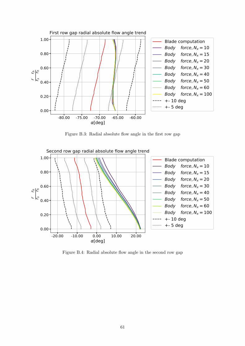
-80.00 -75.00 -70.00 -65.00 -60.00α[deg]

0.00

0.20

0.40

0.60

0.80

1.00r−

r hr s

−r h

First ow gap adial absolute flow angle t endBlade computationBody− force,Nx =10Body− force,Nx =15Body− force,Nx =20Body− force,Nx =30Body− force,Nx =40Body− force,Nx =50Body− force,Nx =60Body− force,Nx =100+- 10 deg+- 5 deg

Figure B.3: Radial absolute flow angle in the first row gap

-20.00 -10.00 0.00 10.00 20.00α[deg]

0.00

0.20

0.40

0.60

0.80

1.00

r−r h

r s−r h

Second row gap radial ab olute flow angle trendBlade computationBody− force,Nx=10Body− force,Nx=15Body− force,Nx=20Body− force,Nx=30Body− force,Nx=40Body− force,Nx=50Body− force,Nx=60Body− force,Nx=100+- 10 deg+- 5 deg

Figure B.4: Radial absolute flow angle in the second row gap

61

-80.00 -75.00 -70.00 -65.00 -60.00α[deg]

0.00

0.20

0.40

0.60

0.80

1.00r−

r hr s

−r h

Near t ailing edge adial absolute flow angle t endBlade computationBody− force,Nx =10Body− force,Nx =15Body− force,Nx =20Body− force,Nx =30Body− force,Nx =40Body− force,Nx =50Body− force,Nx =60Body− force,Nx =100+- 10 deg+- 5 deg

Figure B.5: Radial absolute flow angle near the last blade trailing edge

-80.00 -75.00 -70.00 -65.00 -60.00α[deg]

0.00

0.20

0.40

0.60

0.80

1.00

r−r h

r s−r h

Outlet adial absolute flow angle t endBlade computationBody− force,Nx =10Body− force,Nx =15Body− force,Nx =20Body− force,Nx =30Body− force,Nx =40Body− force,Nx =50Body− force,Nx =60Body− force,Nx =100+- 10 deg+- 5 deg

Figure B.6: Radial absolute flow angle near the outlet

62

References[1] D. K. Hall. “Analysis of civil aircraft propulsors with boundary layer ingestion”.

PhD thesis. Massachusetts Institute of Technology, 2015, pp. 1–116. url:https://dspace.mit.edu/handle/1721.1/97353.

[2] W. Thollet. “Body force modeling of fan – airframe interactions”. PhD thesis. UniversiteFederale Toulouse Midi-Pyrenees, 2017, pp. 1–157.

[3] Olivier Atinault et al. “Numerical and experimental aerodynamic investigations ofboundary layer ingestion for improving propulsion efficiency of future air transport”. In:31st AIAA Applied Aerodynamics Conference June 2013 (2013). doi:10.2514/6.2013-2406.

[4] Alejandra Uranga et al. “Preliminary experimental assessment of the boundary layeringestion benefit for the D8 aircraft”. In: 52nd Aerospace Sciences Meeting January 2017(2014). doi: 10.2514/6.2014-0906.

[5] Jin Guo and Jun Hu. “Development of body force model for steady inlet distortions inhigh-speed multistage compressor”. In: Proceedings of the Institution of MechanicalEngineers, Part G: Journal of Aerospace Engineering 231.9 (2017), pp. 1650–1659. issn:20413025. doi: 10.1177/0954410016656880.

[6] M T Latour. “Modeling axial compressor fan blades using a body force model”.PhD thesis. Delft University of Technology.

[7] F Marble. “Three Dimensional Flow in Turbomachines”. In: High Speed Aerodynamicsand Jet Propulsion X (1964), pp. 83–166.

[8] D. K. Hall, E. M. Greitzer, and C. S. Tan. “Analysis of fan stage conceptual designattributes for boundary layer ingestion”. In: Journal of Turbomachinery 139.7 (2017),pp. 1–10. issn: 15288900. doi: 10.1115/1.4035631.

[9] David J. Hill and Jeffrey J. Defoe. “Innovations in body force modeling of transoniccompressor blade rows”. In: International Journal of Rotating Machinery 2018.1 (2018).issn: 15423034. doi: 10.1155/2018/6398501.

[10] Luis Lopez de Vega, Guillaume Dufour, and Nicolas Garcıa Rosa. “A fully coupled bodyforce-engine performance methodology for boundary layer ingestion”. In: AIAAPropulsion and Energy Forum and Exposition, 2019 August (2019), pp. 1–15. doi:10.2514/6.2019-3828.

63

https://dspace.mit.edu/handle/1721.1/97353

https://doi.org/10.2514/6.2013-2406

https://doi.org/10.2514/6.2014-0906

https://doi.org/10.1177/0954410016656880

https://doi.org/10.1115/1.4035631

https://doi.org/10.1155/2018/6398501

https://doi.org/10.2514/6.2019-3828

Date post:	09-Feb-2022
Category:	Documents
Upload:	others
View:	3 times
Download:	0 times

XQVFKRWHQ - TU Delft

Documents