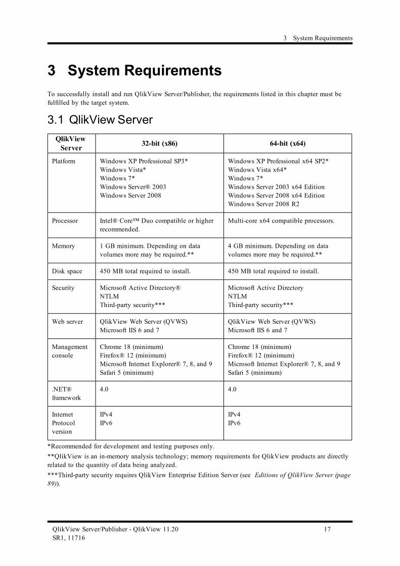
150
Server/Publisher Version 11.20 SR1 for Microsoft Windows® Second Edition, Lund, Sweden, January 2013 Authored by QlikTech International AB

YADE-OPEN DEM: an open–source software using a
discrete element method to simulate granular material
J. Kozicki∗
F.V. Donze†
August 18, 2008
Abstract
Purpose - YADE–OPEN DEM is an open source software based on the Discrete ElementMethod which uses object oriented programming techniques. The paper describes the softwarearchitecture.Design/methodology/approach - The DEM chosen uses position, orientation, velocity andangular velocity as independent variables of simulated particles which are subject to explicitleapfrog time–integration scheme (Lagrangian method). The three–dimensional dynamics equa-tions based on the classical Newtonian approach for the second law of motion are used. Thetrack of forces and moments acting on each particle is kept at every time–step. Contact forcesdepend on the particle geometry overlap and material properties. The normal, tangential andmoment components of interaction force are included.Findings - An effort has been undertaken to extract the underlying object oriented abstractionsin the Discrete Element Method. These abstractions were implemented in C++, conform toobject oriented design principles and use design patterns. Based on that, a software frameworkwas developed in which the abstractions provide the interface where the modelling methodscan be plugged–in.Originality/value - The resulting YADE-OPEN DEM framework is designed in a genericway which provides great flexibility when adding new scientific simulation code. Some of theadvantages are that numerous simulation methods can be coupled within the same frameworkwhile plug–ins can import data from other software. In addition, this promotes code improve-ment through open source development and allows feedback from the community. Howeverimplementing such models requires that one adheres to the framework design and the YADEframework is a new emerging software. To download the software see http://yade.wikia.comwebpage.Keywords Open–Source, Software Design, Generic Programming, Discrete Element Method,SimulationPaper type Research paper
1 Introduction
Granular materials are found much in nature and in various industries. For example, they are foundin landslides and avalanches, raw minerals extraction and transport, cereal storage, powder mix-ing, without forgetting cohesive frictional materials like concrete which are also made of granulates.These materials exhibit a very specific phenomena, that still need a better understanding. They canbe deformed as solid bodies or soils [38], they may have a flow ability corresponding to that of liquids
∗Faculty of Civil and Environmental Engineering, Technical University of Gdansk, Gdansk-Wrzeszcz 80-952, Naru-towicza 11/12, Poland
†Laboratoire Sols, Solides, Structures et Risques, Universite Joseph Fourier, Grenoble Universites, Domaine Uni-versitaire, B.P. 53 - 38041 Grenoble cedex 9, France
1

and a compressibility like that of gases. For this purpose and beside many experimental studies,numerical simulation is increasingly seen as a means to understand and predict their behavior. Sim-ulation has become a common tool in the design and optimization of industrial processes [10]. Thecontinuous increase in computing power is now enabling researchers to implement numerical methodsthat do not focus on the granular assembly as an entity, but rather deduce its global characteristicsfrom observing the individual behavior of each grain [16, 53]. Due to their highly discontinuousnature, one should expect that granular media require a discontinuous simulation method. Indeed,to date the Discrete Element Method (DEM) is the leading approach to those problems. Modelingis straightforward: the grains are the elements, they interact through local, pairwise contacts, yetare also subject to external factors such as gravitation or contacts with surrounding objects, andthey otherwise obey Newton’s laws of motion.
The DEM is a numerical approach where statistical measures of the global behavior of a phe-nomenon are computed from the individual motion and mutual interactions of a large population ofelements. It is commonly used in situations where state–of–the–art theoretical knowledge has notyet provided complete understanding and mathematical equations to model the physical system [19].
Developing a DEM software often causes scientists to focus on marginal problems not relatedto their scientific work, such as: program interface, input/output of data, geometry handling, meshgeneration or visualization of results. One solution is to use existing scientific frameworks, andplug–in one’s own calculation algorithms (eg. Abaqus, Dyna, Adina, PFC3D and others). Howeverthese frameworks rarely give the possibility of combining together different modelling methods suchas FEM, SPH, DEM or other custom simulations. It is often a commercial software which limitsone’s ability to improve/modify existing code–base. In such a case the user has to fight through theobstacles presented by a flawed software [4]. A common solution is to write one’s own home–brewedsoftware to perform simulation. Time constraints often cause this software to be very specific for aparticular problem, and even when released to the public it is difficult to reuse in another application.As a result a large amount of interesting scientific work is lost for example after PhD students defendtheir thesis.
The solution proposed here is to write a framework named YADE–OPEN DEM which will providea stable base for scientists to operate on. Using an open–source development model will allow directfeedback from authors and encourage the scientific community’s participation. By application of aproper software design the valuable work of others will be preserved and reused.
2 Constructing a framework for the Discrete Element Method
The objective is to find a framework solution which is capable of handling various different simulationmodels. To perform this task, the underlying object oriented abstractions are found by means ofanalysis of a Discrete Element Method [8, 9, 12, 15, 16, 34, 36, 40, 41, 45, 49, 50, 54, 55]. Other models,such as Lattice Geometrical Model [27–31] or Finite Element Method [35,37] were also implementedin YADE software [31] but are out of the scope of this paper.
The DEM method was initially developed by Cundall in 1979 [12] for the analysis of rock. It isa numerical model capable of describing the mechanical behavior of assemblies of discrete elements.The proper interactions between elements are defined to account for the mechanical properties ofthe medium. Thus, the macro-mechanical response of the physical material (deformability, strength,dilatancy, strain localization and other) is reproduced by determining the micro-properties of thematerial in the contact interaction forces (see Fig. 5), i.e. normal, tangential and rolling stiffnesses,local friction and non-dimensional plastic coefficient (these quantities are defined below). Thismethod provides new insight into constitutive modeling because the physical processes which governthe constitutive behavior can be understood at the local scale. Discrete Elements can have differentgeometries, but to keep a low calculation cost, the spherical geometry is often chosen and it will bethe case here.
The purpose of the YADE framework is to provide a stable and uniform environment for scientiststo implement computational algorithms for the Discrete Element Method. It allows easy code reuse,
2
Figure 1: Layered structure of YADE framework.
exchange and extensibility, while also providing many common low–level operations, through plug–ins and libraries. Given that, scientists can now focus on their work instead of reinventing the wheelof input/output or display. The YADE framework is divided into several layers shown in Fig. 1. Eachlayer can depend on layers below it. Libraries in the lowest layer are not related to the simulationitself, and can be used by other software.
Starting from the bottom of Fig. 1, the Class Factory is a C++ wrapper for dynamic linkingloader (dlopen(), etc.). It handles loading and unloading plugins given their class name as a string,after which plug–in file on the hard drive is named. Since it works during runtime, it is easy to switchbetween different concrete implementations of currently tested class, such as: different plugins tosolve or detect body interactions, different methods of drawing graphics with OpenGL, or savingresults to xml or binary format – which comes in handy when benchmarking and testing duringdevelopment. Plug–ins are inheriting from the class Factorable.
The Serialization library supports de/serializaing data with random access to class componentsduring the process, easily human readable xml format and support for creation of new formats (liketxt, yaml or binary). With this library it is recommended to inherit from class Serializable to obtainan easy to use serialization interface. In the future the boost::serialization [1] library will beused.
The Math library provides quaternion, vector and small matrices calculus optimized for 3Doperations. OpenGL library provides a C++ wrapper for glut. Other libraries used in the frameworkare: STL [26,33], Boost [1] and QGLViewer [13].
The generic layer in Fig. 1 represents the core of YADE and provides abstract interfaces to allconcepts of scientific simulation: engines, bodies and interactions (see Sect. 3). Class World (seeSect. 6.2) stores the simulated world, counts time, increments iterations and synchronizes threads.The abstract interfaces for GUI and rendering are also here.
The YADE common layer in Fig. 1 contains components commonly used by various simulationtypes (DEM, FEM, Lattice or SPH), like:
• Newton’s law or Hooke’s law,• time integration algorithms (Leapfrog [20], Newmark, Runge–Kutta 4, etc.),• damping methods (eg. Cundall non viscous damping [12]),• collision detection algorithms (eg. Sweep and Prune [11] or Grid Collider),• boundary conditions (imposing translation, applying gravity, etc.),• data classes that store information about bodies or interactions.
3

Figure 2: Simplified schematics of simulation loop.
• Common OpenGL methods for drawing popular geometries,
The specialized layer is based on the common layer. It contains code that cannot be sharedbetween different methods (see Sect. 4). Many specialized packages can exist: Discrete ElementMethod, Finite Element Method or Lattice Geometrical Model. This paper focuses on granularmaterials and only DEM example is explained.
The top layer is a Graphical User Interface and one based on QT is currently provided, alsoGTK, ncurses or even winAPI are possible as plugins. Moreover, a command line interface can beused to perform computations remotely.
3 Abstractions underlying scientific simulation
Consider that the simulation involves bodies between which interactions occur (Fig 2). These inter-actions can be detected and processed by certain computational algorithms and physical rules (whichare engines in YADE). The result of these algorithms can be a moment, a force, a displacement,etc. (class BodyExternalVariables), which in general produce a response that affects body state. Allbodies, interactions and the simulation loop that processes them (engines) are stored inside theWorld class.
Three kinds of data are distinguished:
• bodies,• interactions,• intermediate data.
All algorithms (see Sect. 3.2) are engines, but they have been divided to:
• Command Pattern: Engine,• Multimethods Pattern: EngineFunctor stored inside EngineDispatcher.
3.1 Data classes
The objects of data classes cannot move or interact themselves, as they only contain data. Theirmovement and interaction are handled by the engine classes. The body is represented by six dataclasses: BodyState, BodyStateConstraints, BodyConstitutiveParameters, BodyShape, BodySimplified-Shape and BodyBoundingVolume. They are held inside World using boost::multi index container.The seemingly obvious notion to create a Body class that would hold all six of them proved to bewrong, since a single body can sometimes be described by multiple instances of BodyShape (eg. a DEMcluster) or thousands of bodies can share a single instance of BodyConstitutiveParameters (eg. someare the concrete, others are the reinforcement). The purpose of those six abstract data classes follows(see examples in Fig. 3):
4

Figure 3: Examples of concrete classes that describe a body, their movement is described in Sec-tion 3.2.
BodyState (Bst) – information about a body that changes during the simulation process and isdifferent for each instance of a body in the simulation, like position, velocity, acceleration andmass or inertia.
BodyStateConstraints (Bsc) – information about constraints imposed on a body state. A con-strained value can be eg.: kept at limiting value, determine a body deletion etc. Exampleconstraints include: maximum strain, crossing spatial boundary or a sliding support. Manybodies can use the same constraints or not use constraints at all.
BodyConstitutiveParameters (Bcp) – information about a body that usually does not changeduring the simulation and is the same for many instances of bodies. It is intended to be aninformation used by constitutive laws, like stiffness or cohesion.
BodyShape (Bsh) – the idealized geometrical shape of a body that is simulated: it is used to createa simplified shape, and for display.
BodySimplifiedShape (Bss) – a shape of the body used for performing the actual simulation, maybe different from idealized shape, because it is merely its representation used for the purposeof the simulation.
BodyBoundingVolume (Bbv) – a bounding volume is used to detect potential interaction betweenbodies, usually is built from information stored inside simplified shape.
The interaction is represented by two data classes: InteractionState and InteractionConstitu-tiveParameters. They serve following purposes:
InteractionState (Ist) – information about an interaction happening between bodies which changeswhile the interaction evolves during the simulation (eg.: penetration depth, shearing force, con-tact points or volume of contact V ).
InteractionConstitutiveParameters (Icp) – information about an interaction happening be-tween bodies which usually does not change during the simulation, even when bodies discon-nect and reconnect again (eg.: contact stiffness).
Finally two data classes contain intermediate data, those are: BodyExternalVariables and Out-putData:
BodyExternalVariables (Bex) – this information is an intermediate stage to calculate futurevalues of BodyState for the next execution of simulation loop. Usually it contains the sum ofeffects calculated by some physical rules. For example a sum of forces and moments actingon a sphere is used to change body’s position and orientation. It is discussed separately fromother Body... classes, because it does not describe bodies themselves — just changes to them.
OutputData (Odt) – this data is used to store results that cannot be directly obtained from otherdata classes. Usually some Engine will interpret necessary data and store it here, eg.: anaveraged stress, a number of bodies that fulfill some criterion, etc.
To store all data classes, the boost::multi index container is used. It allows to cross–referenceclass instances and to iterate over data elements with respect to different keys. Eg.: to iterate over
5

Figure 4: Class Engine and example algorithms inheriting from it
all bodies involved in a selected interaction or alternatively to iterate over all interactions in whicha given body takes part — a different view on the very same data.
3.2 Engine classes
Every operation concerning data is performed by a dedicated Engine. Applying boundary condi-tions, moving, creating, modifying, destroying, displaying, loading, saving, calculating, converting,interpreting — all those functions are performed by some specific Engine class. Figure 4 shows someexample classes of two kinds: commands and multimethods.
The Command Pattern classes (deriving from Engine) have some empty subcategories servingto help organize the engines derivation tree. Concrete implementations of algorithms are inheritingfrom them:
EgiConditionApplier (Econ) – performs tasks that depend on conditions from outside, like:applying force as a boundary condition of the simulation or imposing a kinematic translationaccording to data read from file on hard disk.
EgiBoundingVolumeCollider (Ebvc) – detects collisions using various algorithms, eg. Sweepand Prune [11] or Grid Collider,
EgiConstitutiveLaw (Elaw) – the constitutive law for any given calculation method (comparewith Sect. 4), eg. ElawElasticContact used for DEM (Eq. 1–2).
EgiTimeStepper (Etim) – methods for choosing the optimal time step if the simulation is dy-namic, it can be based on maximum velocity of bodies, their mass and stiffnes or other criteria(for example as in [48]).
EgiDataProcessor (Edat) – methods for calculating any results which are to be stored in Out-putData.
Adding more Engine subcategories is implied by design flexibility and will happen during the frame-work evolution.
Addition of new plug–ins operating on data classes is possible by writing only two files: .hpp
and .cpp with short code inside. A convention for naming those plug–ins had to be assumed andeach class starts with a three letter code–name of a class that is on the top of its inheritance tree(eg. Egi for Engine). Those code–names are written above next to the long name, in brackets.
The Multimethods allow implementing different collision algorithms in separate classes. Considerthat a BssSphere collides with another sphere or alternatively with a BssBox. The exact formula for
6

calculating the collision will be different. With the use of multimethods it is ensured that the correctformula is chosen automatically, without the need to modify anything else in the YADE code. Touse it, when implementing formulas for a collision between new BodySimplifiedShape-s (eg. whenadding an ellipsoid to the code), one needs to specify a FUNCTOR2D macro inside a body of the class.The 2D indicates that two shapes are involved (eg. a sphere colliding with an ellipsoid), which meansthat it is a two dimensional multimethod.
This automatic mechanism works on the basis of two following classes:
EngineDispatcher (Ed •) – the dispatcher is implemented in YADE common layer for all variantscurrently used in specialized layers. The • indicates the number of dimensions, most commonlyused are two dimensions.
EngineFunctor (Ef •) – this is a parent class for concrete code used in multimethod pattern, the• indicates the number of dimensions. When writing a new collision formula (as mentioned inabove paragraph), one needs to derive from this class.
Thanks to multimethods each algorithm resides in a separate plug–in class, which increasesmodularity. This solution allows easy modification, debugging and exchanging algorithms whenneeded.
4 Overview of the implemented Discrete Element Method
4.1 Generation of a DEM sample
Various generation methods for solving sphere placement in three dimensions exist, such as dynamiccompaction [15,16], radius growth or by solving geometrical equations for sphere placement [23,24].The obtained specimen has to have the desired porosity and the sphere overlap should be as smallas possible. Currently in YADE the sample is generated by assuming spheres position at random(overlap is allowed) in a volume bigger than the target volume. Then a triaxial compression isperformed with friction and cohesion disabled until desired stress on the walls is obtained, optionallya kinematic radius growth can be used.
This has been implemented in files EgiTriaxialCompression.cpp and GenTriaxialTest.cpp
(which inherits from class Generator). If a need arises to create a different kind of sample configu-ration, a new Generator can be written on the basis of other existing generators.
4.2 DEM formulation
Let two spheres A and B, be in contact. The radii of these spherical elements are rA and rB. Inthe global set of axes, their positions are defined by two vectors ~xA and ~xB. The interaction forcevector ~F which represents the action of element A on element B may be decomposed into a normaland a shear vector ~F n and ~F s respectively, which may be classically linked to relative displacements,through normal and tangential stiffnesses, Kn and Ks.
~F ni = Knun~ni, (1)
∆~F si = −Ks∆~us, (2)
where un is the relative normal displacement between two elements, ~ni is the normal contactvector, ∆~us is the incremental tangential displacement. The shear force ~F s is obtained by summingthe ∆~F s increments.
To reproduce the behavior of non cohesive geomaterials, a Mohr-Coulomb rupture criterion isused:
∣
∣
∣
~F s∣
∣
∣ ≤∣
∣
∣
~F n∣
∣
∣ tanµ, (3)
where µ is the “internal” friction angle.
7

Figure 5: Interaction between two spherical discrete elements with its normal ~F n, shear ~F s andmoment ~M components.
The contact moment is introduced because the representation of the roughness of grains is missingin spherical DEM models, and is calculated using rolling stiffness Kr:
~M = Kr ~V (At A−1
t=c Bt=c B−1
t ), (4)
where At=c and Bt=c are initial orientations of spheres (at the time when the contact was created)
and At and Bt are current orientations of spheres (where symbol˚denotes a quaternion). The ~V (•)function converts from quaternion representation of orientation to a vector:
~V (q(a, b, c, d)) =
x = αb
sin (α/2)
y = αc
sin (α/2)
z = αd
sin (α/2)
, where α = 2 arccos (a) . (5)
where q is a quaternion with components a, bi , cj and dk . In the case where the rotation angleα = 0 the axis of rotation can be anything since no rotation occurs and to avoid division by zerothe zeros are assigned to x, y and z. The contact moment ~M can be further decomposed into“plane of contact” component and “normal of the contact” component, thus representing bendingand twisting respectively, in case different stiffnesses for bending and twisting are desired.
The rolling stiffness parameter Kr defines the level of influence that the resistant moment pro-duces; Let us introduce a dimensionless number βr, which expresses a relationship between Kr andKs, such that,
βr = r2Ks
Kr, (6)
where r is the mean value of the two radii.Let us also introduce ηr as a dimensionless parameter of the elastic limit of rolling, which controls
the elastic limit of the rolling behavior. If∣
∣
∣
~F n∣
∣
∣ represents the norm of the normal force at the contactpoint, the elastic limit is given by the plastic moment vector Mplast such that:
Mplast = ηrr∣
∣
∣
~F n∣
∣
∣ (7)
Whereas the norm of the contact moment∣
∣
∣
~M∣
∣
∣ (Eq. 4) is assumed to be smaller than the plasticlimit Mplast:
∣
∣
∣
~M∣
∣
∣ ≤Mplast (8)
8

Figure 6: Typical responses obtained with triaxial tests for dense (solid lines) and loose (dashedlines) sands.
Since various different contact laws have been developed [6, 8, 15, 34, 36, 45, 49, 54] a YADE userwill probably need to add his own law. This can be done by copying one of the existing contact laws(eg. files ElawElasticContact.cpp and ElawElasticContact.hpp) and editing them according tothe user’s needs. Models currently implemented in YADE include the following features: momenttransfer, shear friction, moment creep, shear creep, Mohr–Coulomb contact with cohesion. New lawsare being added, eg. a capillary contact law is being developed by Scholtes [41–43], a particle fluidinteraction by Chen [9] or a contact law based on local density by Jerier [24].
Newton’s second law of motion describes the motion of each element as the sum of all forcesapplied on this element. The dynamic behavior of the system is solved numerically by a timealgorithm in which the velocities and the accelerations are constant at each time step. The systemevolves and an explicit finite difference algorithm is used to reproduce this evolution. It is the keyfeature of DEM, which makes it possible to follow a non–linear interaction of a large number ofparticles without excessive memory requirements or the need for an iterative procedure.
5 Calibration of the local parameters
The calibration of the local properties of the numerical model to the properties of a real geo–material is conveniently done by comparing simulated and real triaxial tests. For example [3, 39]once calibrated, the predictive capabilities of the numerical model will be checked by simulatingother triaxial tests. For the calibration step, the selected local parameters are: Kn, Ks, Kr (or βr),µ and ηr. Their values will be fixed to reproduce, not only the correct shapes of stress–strain andthe volumetric curves, but also the correct macroscopic values of Young’s modulus E, Poisson’s ratioν, the dilatancy angle ψ, the peak σpeak and the post peak strength σpost peak, see Figure 6.
To do so, one must identify the influence of each local parameter on the macroscopic response.First it was found that the elastic parameters and the rupture parameters can be calibrated sepa-rately, which is in agreement with previous results [7, 44].
9

Figure 7: On the left, dependency of Poisson’s ratio on the ratio α = Ks
Kn, on the right, dependency
of Young modulus on Kn.
Figure 8: Dependency on the value of local friction angle: on the left, deviator stress–strain curves,on the right, volumetric–strain curve.
The local elastic parameters Kn and Ks play a major role in the elastic response. The otherelastic parameter βr has a lower impact (less than 10%) on Young’s modulus E and Poisson’s ratio ν.Thus, Kn and Ks will be set first to calibrate the macroscopic elastic behavior.
For an arbitrary value of Kn, the parameter Ks is set according to chosen value of Poisson’sratio. Then, for a constant α = Ks
Kn, Kn is set such that the desired value of Young’s modulus is
obtained (Fig. 7).Once the local elastic parameters are set, the values of the other local parameters (µ, βr and ηr)
must be determined. First, the local friction angle µ has a major influence on both the peak stressand the dilatancy angle, but a low one on the residual stress (Fig. 8). Because of the low influence ofβr on the dilatancy angle, as it will be seen, µ is chosen to control the dilatancy angle value.
Then, it is observed that βr has little influence on the dilatancy angle (Fig. 9), which confirmsthat using µ to control this macroscopic parameter is an adequate choice. On the other hand, βr
highly affects the stress peak and the residual peak. Then, because of the low influence of ηr and µon the residual peak, as it will also be seen, β is chosen to control the residual peak value.
Finally, ηr has little influence on both the residual stress value and the dilatancy angle (Fig. 10),so that µ and βr can be kept to set these macroscopic values. Fortunately, ηr affects the stress peak.Consequently, ηr can be chosen to set the peak stress value.
10

Figure 9: Dependency on the value of the dimensionless rolling stiffness parameter: on the left,deviator stress–strain curves, on the right, the volumetric–strain curve.
Figure 10: Dependency on the value of the elastic limit of rolling: on the left, of deviator stress–straincurves, on the right, the volumetric–strain curve.
6 Software overview
6.1 Running the software
The YADE software can be downloaded from website http://yade.wikia.com, by either usingthe last release (currently it is version 0.11.1) or the latest subversion (SVN) snapshot. The SVNsnapshot is recommended for potential developers, because it usually contains significant changeswhen compared with the release (unless there was a little time since last release). Currently YADEworks in Linux environment (Ubuntu, Debian, CentOS, RedHat) and is compiled using the GnuCompiler Collection (GCC, g++). For easier installation there is currently a debian package providedon the website, for other linux distributions the respective instructions are provided.
Once the yade executable file is started, a window appears in which one can select which Gener-ator to use for specimen generation. A dozen are available, including the GenTriaxialTest (whichuses a new implementation of DEM formulation, as in Eq. 4), GenTriaxialTestWater (which wasused for calculations in [41–43]) or GenLatticeExample (which was used to perform calculationsin [27–31]). Once the calculation begins, the results (eg. position, velocity, forces) are written to aspecified text file. Those files serve as an input for a plotting software, such as Matlab, Octave orGnuplot.
Alternatively all those tasks can be performed from the command line, without using a graphical
11

interface, in case a supercomputer cluster is available remotely for the researcher. For more compli-cated tasks a built–in python language interpreter can be used. If a graphical interface is used, thenOpenGL display is performed by a separate thread, which is synchronized with the simulation loop.
6.2 Simulation overview
The World class is a top–level object representing the simulated world. It contains both data andthe engines operating on it. The engines are executed by calling sequentially the activated() methodfor each Engine, and if the answer was positive, then calling action(). It is up to the user to specifywhat engines are inside the simulation loop.
When top–level World class is loaded from the file, its initializers are invoked, one after another.Usually a BodySimplifiedShape is generated from provided BodyShape. BodyBoundingVolume isgenerated from BodySimplifiedShape. Even BodyShape can be generated here according to somealgorithm, or by loading it from another file written in different format (eg. exported from netgen,gmsh or some other program that can perform model discretization).
When the simulation is started, engines stored in simulationLoop are executed sequentially.Usually this involves detecting interactions, solving them, applying solution results to bodies andsaving some data to disk.
7 YADE-OPEN DEM framework applied to Discrete Ele-
ment Method
YADE was designed in a way that new simulation models can be added easily and already definedalgorithms reused. The example below describes what had to be implemented in specialized layers toperform simulation with DEM. The algorithms from SDEC software [15,16] were first implemented,but other algorithms could easily be considered [18, 22, 25, 52]. In DEM the contact is describedby the radii of two spheres: r1, r2, the penetration depth d and the normal vector to the contactplane ~n. To allow interaction between the sphere and a non–spherical object, an imaginary mirrorsphere of double radius is created (as proposed by Donze [16]). Following this definition a new classIstSpheresContact was added. Then two different EngineFunctor -s with algorithms to build thiscontact description were added to EngineDispatcher : one to build the contact between two spheresand the other to build the contact between a sphere and a box. This contact description can beused only if at least one object in the contact is a sphere.
A class describing InteractionConstitutiveParameters was added with the name IcpElasticMicrowhich contains information about the contact: normal stiffness, tangential stiffness and rollingstiffness. When a contact occurs, this information is calculated by a dedicated EngineFunctor whichcalculates macro–micro relationship according to the calibration procedure presented in Section 5.
Finally a simulation loop for DEM calculation was built:
• Calculating time step with elastic criterion (the EtimElasticCriterion class),• building a BoundingVolume using an EngineDispatcher with eg. Ef2 BssSphere BbvAxisAlignedBoundingBox• performing collision detection with a Sweep and Prune collider [11] using the previously cal-
culated bounding volumes (the EbvcSweepAndPrune is shown in Fig. 4),• building InteractionState and InteractionConstitutiveParameters (in this case the classes Ist-
SpheresContact and IcpElasticMicro using a 2D EngineDispatcher,• solving interactions with DEM formulation with the class ElawElasticContact which contains
Eq. 1–2,• applying the calculated response (classes BexForce and BexMoment) to the bodies by calcu-
lating their new acceleration and angular acceleration,• and performing the time integration of bodies according to their new acceleration (eg. using a
leapfrog or Runge–Kutta 4 integration method).
12

(a) (b)
Figure 11: Distribution of forces in a two dimensional DEM sample subject to biaxial compression:(a) results obtained from experiments by means of photoelastic analysis [14]; (b) results obtained inYADE’s DEM implementation.
(a) (b)
Figure 12: A three dimensional DEM sample subject to triaxial compression, results obtained inYADE’s DEM implementation: (a) view on aggregates; (b) distribution of forces
13

(b)
(a)
Figure 13: A DEM specimen of concrete (aggregates connected using using cohesive law), subjectto three point bending: (a) specimen’s configuration; (b) forces in bonds between aggregates (red:compression, blue: tension)
This loop directly implements DEM and is repeated until the calculation is terminated.Figures 11–14 show several example simulations done using the YADE framework. The biaxial
compression in two dimensions shown in Fig. 11 is in good agreement with results by Cundall andde Josselin [12, 14]. Figure 12 shows a similar experiment performed in three dimensions. Thedistribution of forces is clearly visible. Figure 13 shows a concrete beam subjected to a three pointbending, the concrete aggregates are using a cohesive law to transfer tensile force. Figure 14 showsa 2 × 10 cm specimen subject to shearing and the resulting change of tangential to normal forceduring the process.
8 Conclusions
The task to find the underlying abstractions of numerical simulation with Discrete Element Methodhas been completed and explained with examples. Each distinct part of the simulation (such as:choice of the time step, time integration, solution of contact forces, collision detection) was put into aseparate class. With this approach it is possible for example to add different shapes (eg. ellipsoids [25]or polyhedrons [18,52,55]) to the simulation just by adding two files with the required formulas forcontact detection and other two files (.cpp and .hpp respectively) for calculation of interactionstate, while the old contact laws can still work with the newly added ellipsoids or polyhedrons(assuming that the contact law is still applicable). Similarly new contact laws can be added onthe basis of existing contact law — by copying the files of a selected contact law and changingits behavior (eg. viscoplastic, viscoelastic, or capillary contact law [41–43]). Implementation ofYADE-OPEN DEM software performed by authors is open–source and can be downloaded fromhttp://yade.wikia.com webpage.
YADE has an already growing user base, and currently investigated are: a capillary law [41–43],a particle–fluid interaction [8, 9], a method to generate composite materials [23, 24], a dry granularflow [17], modelling of concrete under high impact [51] and high confinement [46, 47].
The implementation of DEM [8, 9, 12, 15, 16, 34, 36, 40, 41, 45, 49, 50, 54, 55] and possibly other
14

(a)
(a)
Figure 14: YADE simulation of a granular specimen 10× 2 cm subject to shearing (Young modulusE = 10 Mpa, Poisson’s ratio ν = 0.38, friction angle tan(φ) = 0.45): (a) distribution of forces duringthe shearing process; (b) plot of tangential to normal force (T/N) to the horizontal displacement udivided by speciment height h = 2 cm.
models such as FEM or Lattice Geometrical Model (LGM) [27–31] in a single framework makes thetask of coupling them with each other to be relatively simple. A single framework that containsdifferent models simplifies code exchanges. The YADE framework is flexible, which gives more powerto the user and minimizes obstacles when implementing a new kind of model.
The major idea behind DEM is to circumvent the complexity of a large assembly by consideringinstead many simple elements, the behavior of which can be simulated accurately. Because of thisapproach, DEM requires careful calibration and validation with real experiments in order to producetrustworthy results. This research extends the work done by Peters [38] by making it possible toadd other models like FEM to the same Object Oriented simulation framework.
Acknowledgments
The authors wish to thank the Joseph Fourier University in Grenoble, the Foundation for PolishScience and Technical University in Gdansk for the financial support on this research.
References
[1] Abrahams, D., Garland,J., Dawes, B., Daniel, C., Gregor, D., Maurer, J., Maddock J. andothers. (2007), ”The Boost Library, Boost Consulting”, http://www.boost.org
[2] Alexandrescu, A. (2000) ”Modern C++ Design: Generic Programming and Design PatternsApplied”, Addison-Wesley.
15

[3] Belheine, N., Plassiard, J.P., Donze, F.V., Darve, F. and Seridi, A. (2008), ”Numerical simula-tion of drained triaxial test using 3D discrete element modeling”, Computers and Geotechnics,(in press) doi:10.1016/j.compgeo.2008.02.003
[4] Bobinski, J. (2006), ”Implementation and application of nonlinear concrete models with non-local softening (lang. pl)”, PhD thesis, Gdansk University of Technology.
[5] Burkhardt,R. (1997), UML — ”Unified Modelling Language”, Addison–Wesley
[6] Yang, B., Jiao, Y. and Lei, S. (2006) ”A study on the effects of microparameters on macroprop-erties for specimens created by bonded particles”, Engineering Computations, Vol. 23 No. 6,pp. 607–631
[7] Calvetti F., Viggiani G. and Tamagnini C., ”A numerical investigation of the incrementalnon-linearity of granular soils”, Rivista Italiana di Geotecnica, Special Issue on Mechanics andPhysics of Granular Materials, 2003.
[8] Chen, F., Drumm, E.C. and Guiochon, G. (2007), ”Prediction/Verification of Particle Motion inOne Dimension with the Discrete-Element Method””, International Journal of Geomechanics,ASCE, Vol. 7, Issue 5, pp. 344–352
[9] Chen, F., Drumm, E.C., Guiochon, G., and Suzuki, K. (2008) ”Discrete Element Simulationof 1D Upward Seepage Flow with Particle–Fluid Interaction Using Coupled Open Source Soft-ware”. Proceedings of The 12th International Conference of the International Association forComputer Methods and Advances in Geomechanics (IACMAG) Goa, India, 1–6 October
[10] Cleary,P.W. (2004), ”Large scale industrial DEM modelling”, Engineering Computations,Vol. 21 No. 2/3/4, pp. 169–204.
[11] Cohen, J.D., Lin, M.C., Manocha D. and Ponamgi M.K. (1995), ”I-COLLIDE: An Interactiveand Exact Collision Detection System for Large-Scale Environments”, Symposium on Interac-tive 3D Graphics, Vol. 218, pp. 189–196.
[12] Cundall, P.A. and Strack, O.D. (1979), ”A discrete numerical model for granular assemblies”,Geotechnique, Vol. 29, pp. 47–65.
[13] Debunne, G. ”The QGLViewer Library”, http://artis.imag.fr/Members/Gilles.Debunne/QGLViewer/
[14] De Jong, G.J. and Verruijt, A. (1969), ”Etude photo-elastique d’un empilement de disques”,Cah. Grpe fr. Etud. Rheol, Vol. 2, pp. 73–86.
[15] Donze, F. and Magnier, S.A. (1995), ”Formulation of a three–dimensional numerical model ofbrittle behavior”, Geophys. J. Int., Vol. 122, pp. 790–802.
[16] Donze, F., Magnier, S.A., Daudeville, L., Mariotti, C. and Davenne, L. (1999) ”Numerical studyof compressive behaviour of concrete at high strain rates”, Journal for Engineering Mechanics,Vol. 125, No. 10, pp. 1154–1163.
[17] Favier, L. and Daudon, D. (2008) ”Dry granula flow impact against an obstacle: numericalmodel and laboratory measurements”, Discrete Element Group for Hazard Mitigation, annualreport 4, pp.H1–H15.
[18] Feng, Y.T. and Owen, D.R.J. ”A 2D polygon/polygon contact model: algorithmic aspects”,Engineering Computations, Vol. 21, No. 2/3/4, pp. 265-277
[19] Ferrez, J.A. (2001), ”Dynamic triangulation for efficient 3D simulation of granular mate-rial”(lang. eng), PhD thesis, Ecole Polytechnique Federal de Lausanne.
16
[20] Fincham,D., (1992), ”Leapfrog rotational algorithm”, Molecular Simulations, Vol. 8, No. 3/5,pp 165–178.
[21] Gamma, E., Helm, R., Johnson R. and Vlissides, J. (1995), ”Design Patterns: Elements ofReusable Object–Oriented Software”, Addison-Wesley, ISBN: 0201633612.
[22] Han, K., Feng Y.T. and Owen, D.R.J. (2007), ”Performance comparisons of tree-based and cell-based contact detection algorithms”, Engineering Computations, Vol. 24, No. 2, pp. 165–181.
[23] Jerier, J.F., Donze, F.V. and Imbault, D. (2007) ”An Algorithm to Generate Random Dense Ar-rangements Discs Based on the Triangulation”, Discrete Element Group for Hazard Mitigation,annual report, Vol. 3, pp.D1–D7.
[24] Jerier, J.F., Donze, F.V., Imbault, D. and Doremus P. (2008) ”A geometric algorithm fordiscrete element method to generate composite materials”, Discrete Element Group for HazardMitigation, annual report, Vol. 4, pp.A1–A8.
[25] Johnson, S., Williams, J.R., Cook, B. (2004), ”Contact resolution algorithm for an ellipsoidapproximation for discrete element modeling”, Engineering Computations, Vol. 21, No. 2/3/4,pp. 215-234
[26] Josuttis, N.M. (2000), ”The C++ Standard Library: A Tutorial and Reference”, Addison-Wesley.
[27] Kozicki, J. and Tejchman, J. (2006) ”2D Lattice Model for Fracture in Brittle Materials”,Archives of Hydro–Engineering and Environmental Mechanics, Vol. 53, No. 2, pp. 71–88.
[28] Kozicki, J. and Tejchman, J. (2007),”Effect of aggregate structure on fracture process in concreteusing 2D lattice model”, Archives of Mechanics, Vol. 59, No. 4/5, pp. 365–384.
[29] Kozicki, J. (2007), ”Application of discrete models to describe the fracture process in brittlematerials”, PhD thesis, Gdansk University of Technology.
[30] Kozicki, J. and Tejchman, J. (2008), ”Modelling of fracture process in concrete using a novellattice model”, Granular Matter, DOI 10.1007/s10035-008-0104-4, (in print)
[31] Kozicki, J. and Donze, F.V. (2008),”A new open–source software developed for numerical sim-ulation using discrete modelling methods”, Computer Methods in Applied Mechanics and En-gineering, DOI 10.1016/j.cma.2008.05.023 (in print).
[32] Martin, R.C. (2000),”Design Principles and Design Patterns”, http://www.objectmentor.
com/resources/articles/Principles_and_Patterns.pdf
[33] Meyers,S. (2000), ”Effective STL”, Addison-Wesley.
[34] Morris, J.P., Rubin, M.B., Blair, S.C., Glenn, L.A. and Heuze, F.E. (2004), ”Simulationsof underground structures subjected to dynamic loading using the distinct element method”,Engineering Computations, Vol. 21, No. 2/3/4, pp. 384–408
[35] Munjiza, A. (2004), ”The combined finite-discrete element method”, John Wiley & Sons, Ltd.
[36] Nicot, F., L. Sibille, F.V. Donz and F. Darve, (2007) ”From microscopic to macroscopic second–order work in granular assemblies”, Int. J. Mech. Mater., Vol. 7, No. 39, pp. 664–684
[37] Owen D.R.J. and Feng, Y.T. (2001), ”Parallelised finite/discrete element simulation of multi-fracturing solids and discrete systems”, Engineering Computations, Vol. 18, No. 3/4, pp 557–576.
17

[38] Peters, B. and Dziugys, A.D. (2002), ”Numerical simulation of the motion of granular materialusing object–oriented techniques”, Computer methods in applied mechanics and engineering,Vol. 191, pp. 1983–2007.
[39] Plassiard, J.P., Belheine, N. and Donz, F. (2008), ”A Spherical Discrete Element Model: cali-bration procedure and incremental response”, Granular Matter, (in press).
[40] Rapaport, D.C. (2004) ”The Art of Molecular Dynamics Simulation, second edition”, Cam-bridge, ISBN 0-521-82568-7
[41] Scholtes, L., Chareyre, B., Nicot, F. and Darve, F. (2008) ”Micromechanics of Granular Mate-rials with Capillary Effects”, International Journal of Engineering Science, (in print).
[42] Scholtes, L., Chareyre, B. and Darve, F. (2008) ”DEM modeling of unsaturated granular ma-terials: insight into stress conceptions”, Discrete Element Group for Hazard Mitigation, annualreport 4, pp.D1–D9.
[43] Scholtes, L., Chareyre, B., Nicot, F. and Felix Darve, (2008) ”Capillary Effects Modelling InUnsaturated Granular Materials”, 5th European Congress on Computational Methods in AppliedSciences and Engineering ECCOMAS 2008, Venice, Italy, 30 June — 4 July
[44] Sibille, L., Nicot, F., Donz, F.V. and Darve, F., ”Material instability in granular assemblies fromfundamentally different models”, International Journal For Numerical and Analytical Methodsin Geomechanics, Vol. 31, pp. 457-481, 2007.
[45] Sibille, L., Nicot, F., Donz, F.V. and Darve F. (2007) ”Material instability in granular assem-blies from fundamentally different models”, International Journal For Numerical and AnalyticalMethods in Geomechanics, Vol. 31, pp. 457-481
[46] Shiu, W.J., Donze, F.V. and Daudeville L. (2007) ”Discrete element modelling of missile impactson a reinforced concrete target”. Int. Conf. on Computational Fracture and Failure of Materialsand Structures (CFRAC 2007), Nantes, 11–13 June
[47] Shiu, W.J., Donze, F.V. and Daudeville, L. (2008) ”Compaction process in concrete duringmissile impact: a DEM analysis”, Discrete Element Group for Hazard Mitigation, annual report4, pp.L1–L12.
[48] O’Sullivan, C., Bray, J.D. (2004), ”Selecting a suitable time step for discrete element simulationsthat use the central difference time integration scheme”, Engineering Computations, Vol. 21,No. 2/3/4, pp. 278-303
[49] Tijskens, E., De Baerdemaeker, J. and Ramon H. (2004) ”Strategies for contact resolution oflevel surfaces”, Engineering Computations, Vol. 23, No. 6, pp. 137–150.
[50] Thornton,C. and Zhang, L. (2001), ”A DEM comparison of different shear testing devices(invited lecture)”. Powders and Grains conference, Kishino (ed.).
[51] Tran, V.T., Donze, F.V. and Marin, P. (2008) ”Discrete modeling of concrete under high levelof confinement”, Discrete Element Group for Hazard Mitigation, annual report 4, pp.I1–I12.
[52] Williams, J.R., Perkins, E., and Cook. B. (2004), ”A contact algorithm for partitioning arbitrarysized objects”, Engineering Computations, Vol. 21, No. 2/3/4, pp. 235–248.
[53] Yang, B., Jiao, Y. and Lei, S. (2006), ”A study on the effects of microparameters on macro-properties for specimens created by bonded particles”, Engineering Computations, Vol. 23, No.6, pp. 607–631.
18

[54] Yu, A.B. (2004) ”Discrete element method: An effective way for particle scale research ofparticulate matter”, Engineering Computations, Vol. 21, No. 2/3/4, pp. 205-214
[55] Zhao, D., Nezami, E.G., Hashash, Y.M.A. and Ghaboussi, J. (2006), ”Three-dimensional dis-crete element simulation for granular materials”, Engineering Computations, Vol. 23, No. 7, pp.749–770.
19


