35
YALMIP Yet another LMI parser Version 1.1 JohanL¨ofberg

YALMIP
Yet another LMI parser
Version 1.1
Johan Lofberg

2

Command overview
Category SyntaxWorkspace yalmip(’clear’)
yalmip(’info’)yalmip(’nvars’)
Symbolic variable X = sdpvar(nx,ny,type)y = double(X)see(X)
LMI definition F = lmi(’expression’)F = addlmi(F,’expression’)
Solution of SDP sol = solvesdp(F,G,h,options,x0)options = sdpsettings(parameterlist)
Other & test yalmipdemodbtestsavesdpafile(F,h,’file’)

4

Contents
1 Introduction 7
1.1 Requirements . . . . . . . . . . . . . . . . . . . . . . . . . . . . 7
1.2 Installation . . . . . . . . . . . . . . . . . . . . . . . . . . . . . 7
2 Semidefinite programming and linear matrix inequalities 9
3 Using YALMIP 11
3.1 Examples . . . . . . . . . . . . . . . . . . . . . . . . . . . . . . 11
4 Supported solvers 15
5 Command Reference 19
5.1 Overloaded sdpvar functions . . . . . . . . . . . . . . . . . . . 20
5.2 addlmi . . . . . . . . . . . . . . . . . . . . . . . . . . . . . . . . 21
5.3 lmi . . . . . . . . . . . . . . . . . . . . . . . . . . . . . . . . . . 23
5.4 savesdpafile . . . . . . . . . . . . . . . . . . . . . . . . . . . . . 24
5.5 see . . . . . . . . . . . . . . . . . . . . . . . . . . . . . . . . . . 25
5.6 sdpvar . . . . . . . . . . . . . . . . . . . . . . . . . . . . . . . . 26
5.7 sdp2var . . . . . . . . . . . . . . . . . . . . . . . . . . . . . . . 27
5.8 sdpvarfun . . . . . . . . . . . . . . . . . . . . . . . . . . . . . . 28
5.9 sdpsettings . . . . . . . . . . . . . . . . . . . . . . . . . . . . . 29
5.10 solvesdp . . . . . . . . . . . . . . . . . . . . . . . . . . . . . . . 31

Contents
5.11 updatelmi . . . . . . . . . . . . . . . . . . . . . . . . . . . . . . 33
5.12 yalmip . . . . . . . . . . . . . . . . . . . . . . . . . . . . . . . . 34
Bibliography 35
Index 35
6

1 Introduction
This manual gives an overview of the LMI parser YALMIP (Yet Another LMIParser). The YALMIP package is developed with the aim to have a parserthat is completely integrated and developed in the MATLAB environment.The advantages with this approach is the platform independence and the easeto extend the package with new features. The drawback is of course theperformance loss. The package is therefore intended for small problems with10-100 variables and constraints.
1.1 Requirements
The package uses the object oriented capabilities of MATLAB and thereforeMATLAB 5 or higher is needed. The package is currently used on UNIXMATLAB 6.0 and Windows MATLAB 5.3 without problems.
Since YALMIP works as an interface to the free solvers SP, SOCP, MAXDET,CSDP, SeDuMi, SDPT3 and SDPA, at least one of these packages has to beinstalled on the system.
1.2 Installation
To install YALMIP, unzip the file yalmip.zip in the directory where youwant to have your YALMIP directory. After the installation, you should haveobtained the following directory structure
../yalmip
../yalmip/@lmi
../yalmip/@sdpvar
../yalmip/extras
../yalmip/doc
Put the ../yalmip and ../yalmip/extras directories in your MATLAB path.
The installation of the solvers should be performed as recommended in the

Introduction
respective manuals. Some additional important information concerning theinstallation of the solvers is given in Chapter 4.
8
2 Semidefinite programming andlinear matrix inequalities
In the field of optimization, the crucial property is not linearity but convexity.Recently, there has been much development for problems where the constraintscan be written as the requirement of a matrix to be positive semidefinite. Thisis a convex constraint and motivates the definition of a linear matrix inequality,LMI.
Definition 1 (LMI) An LMI (linear matrix inequality) is an inequality, inthe free scalar variables xi, that for some fixed symmetric matrices Fi can bewritten as
F (x) = F0 + x1F1 + x2F2 + . . . + xnFn � 0
or in a more compact notation
F (x) � 0
In the definition above, we introduced the notion of a semidefinite matrixF � 0 which means F = F T and zT Fz ≥ 0 ∀z.
As an example of an LMI, the nonlinear constraint x1x2 ≥ 1, x1 ≥ 0, x2 ≥ 0can be written [
x1 11 x2
]� 0
The matrix can be decomposed into a set of basis matrices and we obtain
F (x) =[0 11 0
]+ x1
[1 00 0
]+ x2
[0 00 1
]� 0
An excellent introduction to LMIs, with special attention to problems in con-trol theory, can be found in [8].
By using LMIs, many convex optimization problems, such as linear program-ming and quadratic programming, can be unified by the introduction of semidef-inite programming [12].

Semidefinite programming and linear matrix inequalities
Definition 2 (SDP) An SDP (semidefinite program), is an optimization prob-lem that can be written as
minx
cT x
subject to F (x) � 0
SDPs can today be solved with high efficiency, i.e., with polynomial complex-ity, due to the recent development of solvers using interior-point methods [11].One particular solver is [13] which is freely available.
A special class of SDP is MAXDET problems.
Definition 3 (MAXDET) A MAXDET problem (determinant maximiza-tion) is an optimization problem that can be written as
minx
cT x − log det(G(x))
subject to F (x) � 0
G(x) � 0
This is an optimization problem that frequently occurs in problems where theanalysis is based on ellipsoids. A MAXDET problem can be converted to astandard SDP [11], and thus solved with general SDP solvers. However, thereexist special purpose solvers for MAXDET problems [14].
Another special SDP is SOCP [10].
Definition 4 (SOCP) A SOCP (second order cone program) is an optimiza-tion problem with the structure
minx
cT x
subject to ||Aix + bi|| ≤ cTi x + di
This problem can easily be rewritten into an SDP. Due to the special structurehowever, a more efficient method to solve the problem is to use special purposesolvers such as [9].
10

3 Using YALMIP
YALMIP is intended for problems that can be written as
minx
h(x) − log det(G(x))
subject to F (x) � 0
G(x) � 0
Ax = b
The function h(x) is a scalar linear function. In principle, this is the structurethat we saw in the definition of a MAXDET problem. The difference is themore loosely described goal function, and the linear equality constraints.
3.1 Examples
We introduce the basic concepts in YALMIP with two worked examples.
3.1.1 Lyapunov stability
We have a linear system
x(t) = Ax(t)
and our goal is to find positive definite matrix P satisfying
AT P + P T A ≺ 0
Before defining a new problem, it is advised that you clear the internal struc-ture. This is done with the command
>> yalmip(’clear’);
It is not necessary to perform this command, but it cleans up some memorystructures and old solution structures.

Using YALMIP
Defining a symbolic variable is done with the command sdpvar. In our case,we need a symmetric 2x2 matrix
>> P = sdpvar(2,2,’symmetric’);
We are now ready to define the LMIs. To begin with, we create an LMIstructure containing the constraint that P is positive definite
>> F = lmi(’P>0’);
The Lyapunov equation is added to the LMI structure
>> F = addlmi(F,’A’’*P+P’’*A<0’);
Notice the double transpose operator that has to be used inside a string (stan-dard MATLAB notation).
At this point, we are ready to solve our problem. We only search for a feasiblesolution, so one argument is sufficient
>> solution = solvesdp(F);
The variable solution will contain information related to the solution. Thesolution will also be automatically stored and allow us to use the overloadeddouble function to obtain the numerical solution
>> P_feasible = double(P);
The code for the example above is contained in the file manualex1.m.
3.1.2 Model predictive control
As a second example, we formulate a model predictive control problem withYALMIP .
Once again we have a linear system
x(k + 1) = Ax(k) + Bu(k)y(k) = Cx(k)
12

Examples
The goal is to find the control sequence that minimizes a quadratic finitehorizon performance criteria
minu(·|k)
∑N−1j=0 ||y(k + j + 1|k)||2 + ||u(k + j|k)||2
The minimization should be performed under the control constraint
|u(k + j|k)| ≤ 1, j = 0, 1, . . . , N − 1
and the terminal constraint
|y(k + N |k)| ≤ 1
To solve this, we first write the problem in a vector notation. Define thepredicted outputs and the control sequence
Y =
y(k + 1|k)y(k + 2|k)
...y(k + N |k)
, U =
u(k|k)u(k + 1|k)
...u(k + N − 1|k)
By using the linear system model, we can write
Y = Hx(k) + SU
The optimization problem can be written as
mint,U
t
subject to Y T Y + UT U ≤ t|U | ≤ 1|y(N)| ≤ 1
The constraint can be rewritten using a Schur complement and we obtain
mint,U
t
subject to
t Y T UT
Y I 0U 0 I
� 0
|U | ≤ 1|y(N)| ≤ 1
To solve this with YALMIP, we first clear the internal structure
>> yalmip(’clear’);
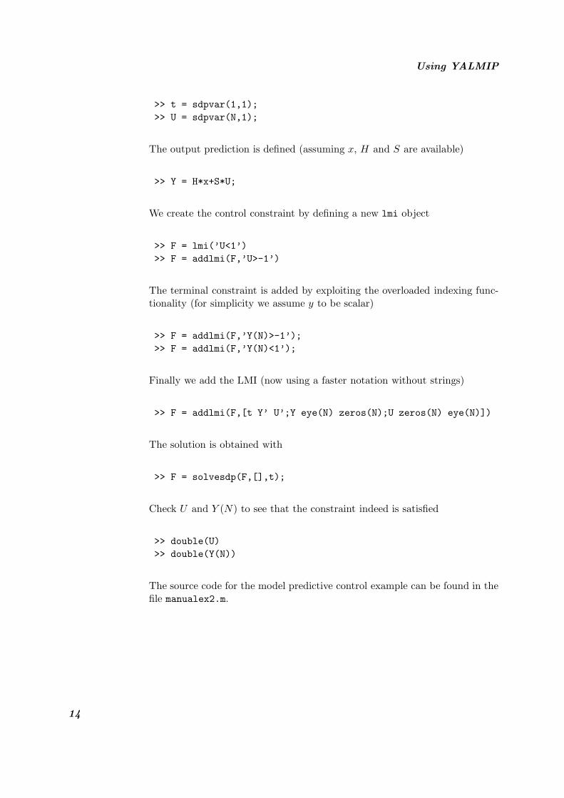
We need two variables
YALMIP 13
Using YALMIP
>> t = sdpvar(1,1);>> U = sdpvar(N,1);
The output prediction is defined (assuming x, H and S are available)
>> Y = H*x+S*U;
We create the control constraint by defining a new lmi object
>> F = lmi(’U<1’)>> F = addlmi(F,’U>-1’)
The terminal constraint is added by exploiting the overloaded indexing func-tionality (for simplicity we assume y to be scalar)
>> F = addlmi(F,’Y(N)>-1’);>> F = addlmi(F,’Y(N)<1’);
Finally we add the LMI (now using a faster notation without strings)
>> F = addlmi(F,[t Y’ U’;Y eye(N) zeros(N);U zeros(N) eye(N)])
The solution is obtained with
>> F = solvesdp(F,[],t);
Check U and Y (N) to see that the constraint indeed is satisfied
>> double(U)>> double(Y(N))
The source code for the model predictive control example can be found in thefile manualex2.m.
14

4 Supported solvers
YALMIP supports a number of different semidefinite programming solvers.However, the level of support differs for the solvers. In this chapter, we give ashort description on the interface to the solvers.
SP
Support : YALMIP was originally developed for SP [13, 7]. Since SP hasbeen the main solver since the beginning, the interface to SP is fully supported.
Status : The SP interface has been extensively tested on both Solaris andWindows.
Installation : Make sure that the SP library is in your MATLAB path.
MAXDET
Support : The MAXDET [14, 2] solver has also been supported by YALMIP fromthe beginning and is fully supported.
Status : The MAXDET interface has been tested extensively on both Solarisand PC.
Installation : Make sure that the MAXDET directory is in your MATLAB path.For Windows versions, it is important that the additional dlls MKL, BLASand LAPACK (explained in the installation information for MAXDET) are inthe Windows path. A simple way to guarantee that everything works is toplace these dlls in the same directory as the solvers.
SOCP
Support : The interface to the SOCP [9, 6] solver has also been a part ofYALMIP since the beginning. YALMIP supports all features of SOCP.

Supported solvers
Status : The SOCP interface has been tested on Solaris.
Installation : Make sure that the SOCP directory is in your MATLAB path.
SeDuMi
Support : The SeDuMi [5] solver is partially supported from version 1.1 ofYALMIP. Currently, YALMIP does not exploit the possibility to solve secondorder cone programs with the specialized code in SeDuMi.
Status : The SeDuMi interface has been tested for a number of problems onboth Solaris and PC.
Installation : Make sure that the SeDuMi directory is in your MATLAB path.
CSDP
Support : The CSDP solver [1] is partially supported from version 1.1 ofYALMIP. No options structure is available for for the CSDP solver. Note thatthe communication with CSDP is done by writing the problem data to a file.Therefore, for large problems, much time will be spent in reading and writingthe problem definition.
Status : The CSDP interface has been tested for a small number of problemson Solaris.
Installation : Make sure that the CSDP directory is in your MATLAB path.Furthermore, a file named csdp.m should be placed in the same directory theCSDPexecutable.
SDPT3
Support : The SDPT3 [4] solver is fully supported from version 1.1 ofYALMIP. The communication with SDPT33 is done by writing the problemdata to a file, hence performance will suffer for large problems.
Status : The SDPT3 interface has been tested for a small number of problemson Windows.
Installation : Make sure that the SDPT3 directory is in your MATLAB path.
16

SDPA
Support : The SDPA [3] solver is partially supported from version 1.1 ofYALMIP. The options structure is currently not used, hence all problems willbe solved with the default settings (found in the file parameters.m in theSDPA directory). The communication also for SDPA is done by writing theproblem data to a file.
Status : The SDPA interface has been tested for a small number of problemson Solaris.
Installation : Make sure that the SDPA directory is in your MATLAB path.Furthermore, a file named sdpa.m should be placed in the same directory asthe SDPAexecutable.
YALMIP 17

Supported solvers
18

5 Command Reference

Command Reference
5.1 Overloaded sdpvar functions
Description Most operators and functions necessary to describe symbolic variables (sdpvarobjects) are overloaded to the sdpvar class.
Examples Addition, subtraction and multiplication are the most basic overloaded func-tions. Assuming X and Y to be sdpvar objects and A to be a double, thefollowing code is valid (assuming sizes are compatible)
>> X = A*Y+X
Standard linear operators such as diag, trace, sum and many more are ofcourse also overloaded
>> X = A*diag(Y)+sum(trace(Y))
Concatenation and indexing can also be used
>> X = Y(1:2,1:2)+[X(end,end) Y(1,1);X(3,1:2)]
Finally, note that multiplication of sdpvar is possible as long as all nonlinearterms disappear. As an example (x and y scalar sdpvar objects)
>> [x 1]*[1;y]
is valid, but not
>> [x 1]*[y;1]
The complete list of overloaded functions are plus, minus, times, mtimes,mrdivide, transpose, ctranspose, trace, diag, blkdiag, repmat, triutril, rot90, flipud, fliplr, sum,diff, kron size, length, horzcat, vertcat,subasgn, subsref, double, display
See Also sdpvar
20

addlmi
5.2 addlmi
Purpose addlmi adds a constraint to an existing LMI object.
Synopsis F = addlmi(G,X);
Description addlmi is used to add constraints on a matrix variable. Both equalities andinequalities are supported, as well as matrix constraints and element-wise con-straints. Furthermore, a special constraint to identify second order constraintsis supported.
G LMI object.
X New constraint, given either as an sdpvar object required to be positivesemidefinite (element-wise non-negative if unsymmetric), or as a stringsymbolically describing the constraint.
Examples Adding the constraint[1 xT
x I
]� 0 (x sdpvar object in Rn)
to an existing LMI structure F is done with
>> F = addlmi(F,’[1 x’’;x eye(n)]<0’)
Another variant is to skip the string notation and use an sdpvar object instead.
>> F = addlmi(F,-[1 x’;x eye(n)])
Notice the sign that has to be used since default is positive semidefiniteness.
Constraints are interpreted as element-wise if an . is used in front of thequantifier. As an example, requiring all elements to be positive is done with
>> F = addlmi(F,’x.>0’)
Second order cone constraints can be added with the special purpose ||·||operator
YALMIP 21

Command Reference
>> F = addlmi(F,’||A*x+b||<c*x+d’)
For the expression to make sense, the expression A*x+b must be a vector, andc*x+d must evaluate to a scalar.
Equality constraints can also be added. A constraint that the sum of thevector components is equal to 1 is obtained with
>> F = addlmi(F,’sum(x)=1’)
See Also lmi , sdpvar
22

lmi
5.3 lmi
Purpose lmi creates a new LMI object.
Synopsis F = lmi(X);
Description lmi creates a creates an LMI object containing the constraint described by X.An empty lmi object is generated if lmi is called without any in-data.
X Constraint, given either as an sdpvar object required to be positive semidef-inite (element-wise non-negative if unsymmetric), or as a string symbol-ically describing the constraint.
Examples See examples in addlmi .
See Also addlmi , sdpvar
YALMIP 23

Command Reference
5.4 savesdpafile
Purpose sdp2mat writes the problem to a file in the SDPA format.
Synopsis savesdpafile(F,h,file);
Description Many solvers are capable of reading problem definitions in the SDPA format,so this function allows the user to use any prefered solver.
F lmi object. The LMIs in the problem.
h sdpvar object. Describes the objective function.
file A string with a filename. If omitted, a dialog box will appear.
See Also lmi , sdpvar
24

see
5.5 see
Purpose sdpvar shows the internal base matrices used to define an sdpvar object.
Synopsis see(X);
Description Every symbolic variable is represented with a set of basis matrices (see defini-tion of LMI). These matrices can be displayed using the see command.
X sdpvar object.
See Also sdpvar
YALMIP 25
Command Reference
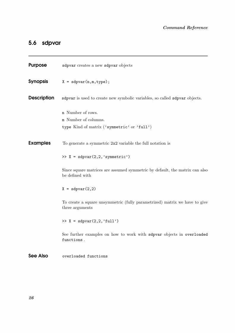
5.6 sdpvar
Purpose sdpvar creates a new sdpvar objects
Synopsis X = sdpvar(n,m,type);
Description sdpvar is used to create new symbolic variables, so called sdpvar objects.
n Number of rows.
m Number of columns.
type Kind of matrix (’symmetric’ or ’full’)
Examples To generate a symmetric 2x2 variable the full notation is
>> X = sdpvar(2,2,’symmetric’)
Since square matrices are assumed symmetric by default, the matrix can alsobe defined with
X = sdpvar(2,2)
To create a square unsymmetric (fully parametrized) matrix we have to givethree arguments
>> X = sdpvar(2,2,’full’)
See further examples on how to work with sdpvar objects in overloadedfunctions .
See Also overloaded functions
26

sdp2var
5.7 sdp2var
Purpose sdp2mat converts the internal solution formats to double.
Synopsis Y = sdp2mat(X,sol);
Description sdp2mat is used to obtain the numerical value from a specific solution. Mostoften, the command double is used.
X sdpvar object.
sol Solution structure.
See Also overloaded functions
YALMIP 27

Command Reference
5.8 sdpvarfun
Purpose sdp2mat applies linear unary function on sdpvar object.
Synopsis Y = sdpvarfun(X,fun);
Description sdp2mat is used to apply any linear unary (one input,one output) matrixoperator on a sdpvar object.
X sdpvar object.
fun string with function name.
Examples To obtain the trace of a sdpvar object (of course, trace is already availableas an overloaded operator, this code is only to examplify the command)
>> Y = sdpvarfun(X,’trace’)
See Also overloaded functions
28

sdpsettings
5.9 sdpsettings
Purpose sdpsettings creates an options structure to be used in solvesdp
Synopsis ops = sdpsettings(parameter,value,parameter,value,...)
Description sdpsettings creates a structure containing the parameters needed in thesolvers. By calling the functions without any argument, the default valuesare obtained.
variable String with parameter name.
value Numerical value of parameter.
Examples To create a structure with default settings
>> ops = sdpsettings>>ops =>>>> Solver: ’’>> Silent: 0>> SaveSolverOutput: 0>> sp: [1x1 struct]>> maxdet: [1x1 struct]>> socp: [1x1 struct]>> sdpt3: [1x1 struct]>> sdpa: [1x1 struct]>> sedumi: [1x1 struct]
The three first parameters are general settings for YALMIP. Solver allowsthe user to explicitely force a specific solver to be used
>> ops = sdpsettings(’Solver’,’SP’);
By default, the solvers operate in silent mode (no printing). This is chosenwith Silent. By setting SaveSolverOutput to 1, all output from the solverswill be saved in the solution structure (see solvesdp).
The options structure also contains a number of structures with parametersused in each supported solver. As an example, the following parameters canbe tuned for the SP solver
YALMIP 29

Command Reference
>> ops.sp>>ans =>>>> AbsTol: 1.0000e-05>> RelTol: 1.0000e-05>> nu: 30>> tv: -Inf>> Mfactor: [50000 1.1000]>> NTiters: 50
See Also solvesdp
30

solvesdp
5.10 solvesdp
Purpose solvesdp solves the semidefinite program
Synopsis solution = solvesdp(F,G,h,ops,x0);
Description solvesdp is the interface to the solvers SP, MAXDET and SOCP.
F LMI object.
G LMI object.
h Linear objective function. See the example for description.
ops Structure holding parameters used in the solvers.
x0 A feasible initial solution. See the example for description.
Examples Let us create an extremely simple problem
min x(1) + x(2), x(1) ≥ 0, x(2) ≥ 0
We clear the internal structures and set up the variables and the constraints
>> yalmip(’clear’);>> x = sdpvar(2,1);>> F = lmi(’x>0’);
Let us start by just finding a feasible solution.
>> sol = solvesdp(F);
If we want to find an optimal solution we must use at least three arguments.Since there is no G(x) term, we let G be an empty matrix
>> sol = solvesdp(F,[],x(1)+x(2));
Notice how easy we defined the objective. Another way is to use a notationthat is more similar to that used in the solvers
>> sol = solvesdp(F,[],[1 1]);
YALMIP 31

Command Reference
This way to define the objective is not recommended since it requires knowl-edge of how the sdpvar object x relates to the internal free variables inYALMIP. However, for the advanced user it might be of interest since it re-moves the need for parsing, hence speeding things up a bit.
Finally, we solve the problem again, but this time we give an initial feasiblesolution. This can be done in two ways. The first method appends a list ofvariables and numerical values to the input argument
>> sol = solvesdp(F,[],sum(x),[],x(1),1,x(2),1);
The important thing is that initial values are given to all free variables. Thefollowing command does the same thing
>> sol = solvesdp(F,[],sum(x),[],x,[1;1]);
Once again, with knowledge of the internal structure, the initial feasible solu-tion can be given as one vector
>> sol = solvesdp(F,[],sum(x),[],[1;1]);
In all the three examples above, the options structure was omitted and anempty matrix was passed. When this is done, the default parameter valuesare used.
Now, let us solve a MAXDET problem
min t − log det(t), t ≥ 0
This is solved with
>> t = sdpvar(1,1);>> F = lmi(’t>0’);>> G = lmi(’t>0’);>> sol = solvesdp(F,G,t);
The optimal solution is saved directly internally, and the numerical values canbe found with the overloaded double function
>> topt = double(t);
See Also overloaded functions , lmi , addlmi sdpvar sdpsettings
32

updatelmi
5.11 updatelmi
Purpose updatelmi updates a symbolic LMI with current numerical values.
Synopsis F = uppdatelmi(F,n);
Description updatelmi is used to change symbolic lmi objects. When a symbolic LMI isdefined, the LMI is immediately converted to a internal numerical representa-tion. By using updatelmi, the symbolic expression is re-evaluated using thecurrent numerical values in the workspace.
F LMI object.
n LMI which should be updated.
Examples Suppose we have a scalar variable t and the constraint[t xx 1
]� 0
and we want to minimize t for the two cases x = 1 and x = 2. This is donewith
>> t = sdpvar(1,1);>> x = 1;>> F = lmi(F,’[t x;x 1]>0’)# 1 :[t x;x 1]>0 Matrix inequality>> solvesdp(F,[],t);t1 = double(t);>> x = 2;>> F = updatelmi(F,1)>> solvesdp(F,[],t);t2 = double(t);
See Also lmi , addlmi
YALMIP 33

Command Reference
5.12 yalmip
Purpose yalmip performs a number of administrative tasks.
Synopsis yalmip(’clear’)yalmip(’info’)n = yalmip(’nvars’)
Description sdpsettings serves as an interface to some internal structures used by theYALMIP package.
Examples Before a new problem is defined, it is advised that the internal structures arecleared
>> yalmip(’clear’)
To find out how many free variables there currently are in all sdpvar objects
>> yalmip(’nvars’)
To get some more information about the current status
>> yalmip(’info’)
See Also solvesdp , sdpvar
34

Bibliography
[1] CSDP. http://www.nmt.edu/ borchers/csdp.html.
[2] MAXDET. http://www.stanford.edu/~boyd/maxdet/.
[3] SDPA. ftp://ftp.is.titech.ac.jp/pub/OpRes/software/SDPA/.
[4] SDPT3. http://www.math.nus.edu.sg/~mattohkc/.
[5] SeDuMi. http://fewcal.kub.nl/sturm/software/sedumi.html.
[6] SOCP. http://www.stanford.edu/~boyd/SOCP/.
[7] SP. http://www.ee.ucla.edu/~vandenbe/sp/.
[8] S. Boyd, L. El Ghaoui, E. Feron, and V. Balakrishnan. Linear MatrixInequalities in System and Control Theory. SIAM Studies in AppliedMathematics. SIAM, Philadelphia, Pennsylvania, 1994.
[9] M. S. Lobo, L. Vandenberghe, and S. Boyd. SOCP : Software for Second-order Cone Programming - User’s Guide. Information Systems Labora-tory, Electrical Engineering Departement, Stanford University, beta ver-sion edition.
[10] M.S. Lobo, L. Vandenberghe, S. Boyd, and H. Lebret. Applications ofsecond-order cone programming. Linear Algebra and its Applications,284:193–228, 1998.
[11] Y. Nesterov and A. Nemirovskii. Interior-Point Polynomial Algorithmsin Convex Programming. SIAM Studies in Applied Mathematics. SIAM,Philadelphia, Pennsylvania, 1993.
[12] L. Vandenberghe and S. Boyd. Semidefinite programming. SIAM Review,38:49–95, March 1996.
[13] L. Vandenberghe and S. Boyd. SP - Software for Semidefinite Program-ming. Information Systems Laboratory, Electrical Engineering Departe-ment, Stanford University, version 1.0 edition, 1998.
[14] S.P. Wu, L. Vandenberghe, and S. Boyd. MAXDET -Software for De-terminant Maximization Problems - User’s Guide. Information SystemsLaboratory, Electrical Engineering Departement, Stanford University, al-pha version edition.


