Yield Curves and

Term Structure Theory

Yield curve

The plot of yield on bonds of the same credit quality andliquidity against maturity is called a yield curve.

Remark The most typical shape of a yield curve has a upwardslope.

The relationship between yields on otherwise comparablesecurities with different maturities is called the termstructure of interest rates.

Year to maturity

Yield

Ideally, yield curve should be plotted for bonds that are alike inall respects other than the maturity; but this is extremelydifficult in practice. Bonds that have similar risks of defaultmay be different in coupon rates, marketability, callability, etc.

Benchmark interest rate or base interest rate

Yield curve on US Treasury bond instruments is used to serveas a benchmark for pricing bonds and to set yields in othersectors of the debt market. This is because the US Treasurybonds are viewed as default free and they have the highestliquidity.

Yield spread and risk premium

On Sept 19, 1997, the yield on the Wal-Mart Stores bonds(rated AA) with 10 years to maturity was 6.476%. On thesame date, the yield on the 10 year most recently issuedTreasury was 6.086%.

Yield spread = 6.476% − 6.086% = 0.39%.

This spread, called a risk premium, reflects the additional risksthe investor faces by acquiring a security that is not issued bythe US Government.

Term structure theory addresses how interest rates are chargeddepends on the length of time that the funds are held.

Spot rateSpot rate is the yield on a zero-coupon Treasury security withthe same maturity.

Any bond can be viewed as a package of zero-couponinstruments. It is not appropriate to use the same interest rateto discount all cash flows arising from the bond. Each cashflow should be discounted at a unique interest rate that isappropriate for the time period in which the cash flow will bereceived. That rate is the spot rate.

Example

A bank offers to depositors one-year spot rate of 4.5% and two-year spot rate of 5%.

That is, if you deposit $100 today, you receive

(i) $104.5 in the one-year deposit one year later;

(ii) (1.05)2 × $100 = $110.25 in the two-year deposit two years

later.

Example

Given the spot rate curve for Treasury securities, find the fairprice of a Treasury bond.

An 8% bond maturing in 10 years (par value = $100).

Each cash flow is discounted by the discount factor for its

time. For example, the discount factor of the coupon paid 8

years later is

Year 1 2 3 4 5 6 7 8 9 10Total present value

spot rate (%) 5.571 6.088 6.555 6.978 7.361 7.707 8.020 8.304 8.561 8.793discount factor 0.947 0.889 0.827 0.764 0.701 0.641 0.583 0.528 0.477 0.431cash flow 8 8 8 8 8 8 8 8 8 108present value 7.58 7.11 6.61 6.11 5.61 5.12 4.66 4.23 3.82 46.50 97.34

.528.0)08304.1(

18

≈

Example (construction of a zero-coupon instrument)

Bond A: 10-year bond with 10% coupon; PA = $98.72.

Bond B: 10-year bond with 8% coupon; PB = $85.89.

Both bonds have the same par of $100.

Construct a portfolio of –0.8 unit of bond A and 1 unit of bondB. Resulting face value is $20, and price is PA − 0.8 PB = 6.914.

The coupon payments cancel, so this is a zero coupon portfolio.The 10-year spot rate is given by

(1 + S10)10 × $6.914 = $20

giving S10 = 11.2%.

Construction of spot rate curve• The obvious way to determine a sport rate curve is to find the

prices of a series of zero-coupon bonds with various maturitydates. However, “zero” with long maturities are rare.

• The spot rate curve can be determined from the prices ofcoupon-bearing bonds by beginning with short maturities andworking forward toward longer maturities.

Example

Consider a two-year bond with coupon payments ofamount C at the end of each year. The price is P2 and thepar value is F. Since the price should equal to thediscounted value of the cash flow stream

where S1 and S2 are the spot rates for one-year period andtwo-year period, respectively.

221

2 )1(1 S

FC

S

CP

+++

+=

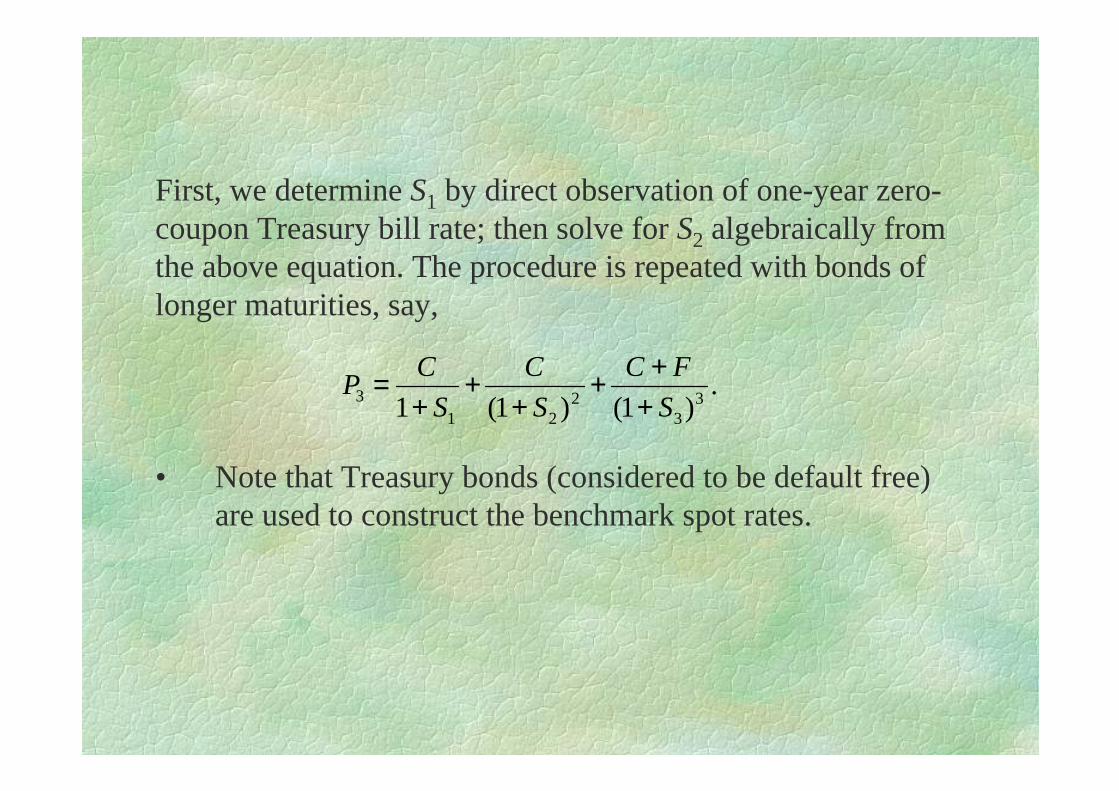
First, we determine S1 by direct observation of one-year zero-coupon Treasury bill rate; then solve for S2 algebraically fromthe above equation. The procedure is repeated with bonds oflonger maturities, say,

• Note that Treasury bonds (considered to be default free)are used to construct the benchmark spot rates.

.)1()1(1 3

32

213 S

FC

S

C

S

CP

+++

++

+=

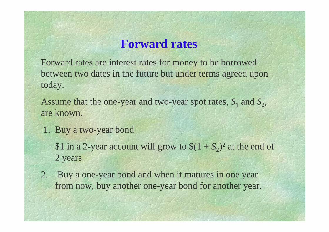
Forward ratesForward rates are interest rates for money to be borrowedbetween two dates in the future but under terms agreed upontoday.

Assume that the one-year and two-year spot rates, S1 and S2,are known.

1. Buy a two-year bond

$1 in a 2-year account will grow to $(1 + S2)2 at the end of2 years.

2. Buy a one-year bond and when it matures in one year from now, buy another one-year bond for another year.

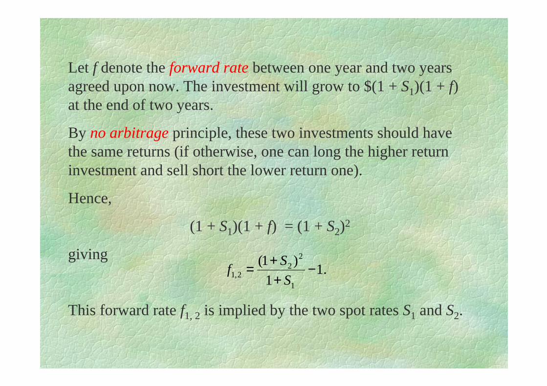
Let f denote the forward rate between one year and two yearsagreed upon now. The investment will grow to $(1 + S1)(1 + f)at the end of two years.

By no arbitrage principle, these two investments should havethe same returns (if otherwise, one can long the higher returninvestment and sell short the lower return one).

Hence,

(1 + S1)(1 + f) = (1 + S2)2

giving

This forward rate f1, 2 is implied by the two spot rates S1 and S2.

.11

)1(

1

22

2,1 −+

+=S

Sf

Forward rate formulasThe implied forward rate between times t1 and t2 (t2 > t1) is the rate ofinterest between those times that is consistent with a given spot ratecurve.

(1) Yearly compounding

giving

(2) Continuous compounding

so that

ijfSS ijji

ii

jj >++=+ − ,)1()1()1( ,

.1)1(

)1()/(1

, −

++

=−ij

ii

jj

ji S

Sf

)( 122,11122ttftStS tttt eee

−=

.12

12 12

21 tt

tStSf tt

tt −−

=

Most spot rate curves slope rapidly upward at short maturitiesand continue to slope upward but more gradually as maturitieslengthen.

Three theories are proposed to explain the evolution of spot ratecurveS:

1. Expectations;

2. Liquidity preference;

3. Market Segmentation.

Determinants of term structure of interest ratesSpot rate

Years

Expectations theoryFrom the spot rates S1,…., Sn for the next n years, we candeduce a set of forward rates f1,2 ,.., f1,n. According to theexpectations theory, these forward rates define the expectedspot rate curves for the next year.

For example, suppose S1 = 7%, S2 = 8%, then

Then this value of 9.01% is the market’s expected value of nextyear’s one-year spot rate .

11

11 ,, −nSS !

%.01.9107.1

)08.1( 2

2,1 =−=f

'1S

Turn the view around: The expectation of next years curvedetermines what the current spot rate curve must be. That is,expectations about future rates are part of today’s market.

Weakness

According to this hypothesis, then the market expects rates toincrease whenever the spot rate curve slopes upward.Unfortunately, rates do not go up as often as expectations wouldimply.

Liquidity preference• For bank deposits, depositors usually prefer short-term

deposits over long-term deposits since they do not like to tie

up capital (liquid rather than tied up). Hence, long-term

deposits should demand high rates.

• For bonds, long-term bonds are more sensitive to interest rate

changes. Hence, investors who anticipate to sell bonds

shortly would prefer short-term bonds.

Market segmentationThe market for fixed income securities is segmented bymaturity dates.

• To the extreme, all points on the spot rate curves are mutually independent. Each is determined by the forces ofsupply and demand.

• A modification to the extreme view is that adjacent ratescannot become grossly out of line with each other.

Expectations DynamicsThe expectations implied by the current spot rate curve willactually be fulfilled.

• To predict next year’s spot rate curve from the currentone under the above assumption. Given S1,…,Sn as the currentspot rates, how to estimate next year’s spot ratesRecall that the current forward rate f1,j can be regarded as theexpectation of what the interest rate will be next year, that is,

.,,, '1

'2

'1 −nSSS !

.11

)1()1/(1

1,1

'1 −

+

+==

−

−

jjj

jj S

SfS

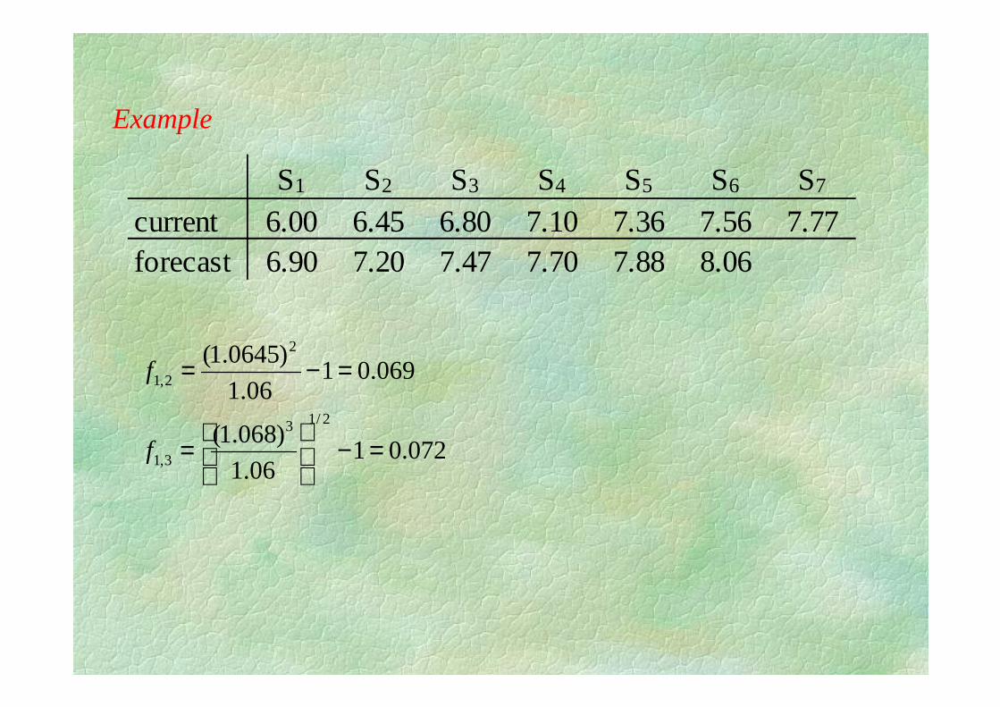
Example

S1 S2 S3 S4 S5 S6 S7

current 6.00 6.45 6.80 7.10 7.36 7.56 7.77forecast 6.90 7.20 7.47 7.70 7.88 8.06

072.0106.1

)068.1(

069.0106.1

)0645.1(

2/13

3,1

2

2,1

=−

=

=−=

f

f

Invariance theorem

Suppose that interest rates evolve according to theexpectation dynamics. Then a sum of money invested inthe interest rate market for n years will grow by a factor

(1 + Sn)n, independent of the investment and reinvestmentstrategy (so long as all funds are fully invested).

This is not surprising since every investment earns therelevant short rates over the period of investment (shortrates do not change under the expectations dynamics).

To understand the theorem, take n = 2.

1. Invest in a 2-year zero-coupon bonus;

2. Invest in a 1-year bond, then reinvest the proceed at the end of the year.

The second strategy would lead as a growth of

the same growth as that of the first strategy.

;)1(1

)1()1()1)(1( 2

21

22

12,11 SS

SSfS +=

+

++=++

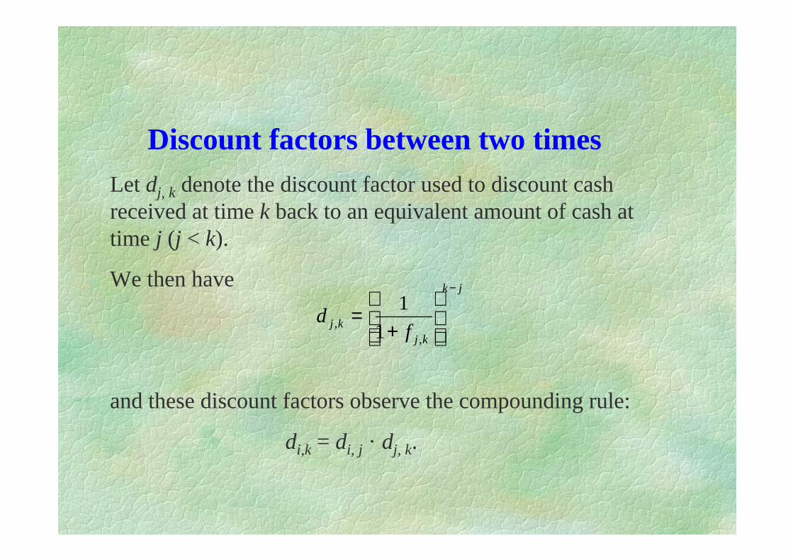
Discount factors between two timesLet dj, k denote the discount factor used to discount cashreceived at time k back to an equivalent amount of cash attime j (j < k).

We then have

and these discount factors observe the compounding rule:

di,k = di, j · dj, k.

jk

kjkj f

d

−

+

=,

, 1

1

Short ratesShort rates are the forward rates spanning a single timeperiod. The short rate at time k is rk = fk, k+1.

The spot rate Sk and the short rates r0, …, rk−1 are related by

(1 + Sk)k = (1 + r0) (1 + r1) … (1 + rk−1)

In general,

(1 + fi, j)j−i = (1 + ri) (1 + ri+1) … (1 + rj−1).

The short rate for a specific year does not change (in thecontext of expectations dynamics).