* Corresponding authors. 1 Dynardo GmbH. 2 Shell Exploration and Production Company. Dynardo Technology and Applications to Well Completion Optimization for Unconventionals Johannes Will *1 and Taixu Bai *2 Stefan Eckardt 1 , Dahai Chang 2 , Ed Lake 2 Abstract The success of an unconventional hydrocarbon development depends on the effective stimulation of reservoir rocks. Industry practice is to conduct a large number of field trials requiring high capital investment and long cycle-time. The workflow and toolkits outlined in this paper offers a cheaper and faster alternative approach to optimizing the completion design for EUR (Estimated Ultimate Recovery) improvement. The approach incorporates subsurface impacts to well stimulation design by employing subsurface parameters, and utilizes well diagnostic and well performance data to calibrate and constrain the models. It integrates subsurface characteristics, well, completion, operation, diagnostic, and well performance analysis. Using asset specific data, it is able to develop an optimal completion design with a set of prioritized completion and operation parameters. This results in reducing the number of field trials for achieving the optimal completion design. In addition, it provides valuable insights for further data acquisition to evaluate and forecast well performance. Field trials based on the results from this approach have yielded encouraging production uplifts with quality forecasts. We believe it is technically feasible to derive an optimal completion design using a subsurface based forward modeling approach that will deliver significant value to the industry. Introduction Unconventional reservoirs produce substantial quantities of oil and gas. These reservoirs are usually characterized by ultra-low matrix permeability. Most unconventional reservoirs are hydraulically fractured in order to establish more effective flow from the reservoir and fracture networks to the wellbores. The success of hydraulic fracture stimulation in horizontal wells has the potential to dramatically change the oil and gas production landscape across the globe and the impacts will endure for decades to come. For a given field development project, the economics are highly dependent completion establishing effective and retained contact with the hydrocarbon bearing rocks. Well and completion design parameters that influence the economic success of the field development include well orientation and landing zone, stage spacing and perforation cluster spacing, fluid volume, viscosity and pumping rate, and proppant volume, size and ramping schedule. Optimization of these design parameters to maximize asset economic value is key to the success of every unconventional asset.
Transcript
*Corresponding authors. 1Dynardo GmbH. 2Shell Exploration and Production Company.
Dynardo Technology and Applications to Well Completion Optimization for Unconventionals
Johannes Will*1 and Taixu Bai*2
Stefan Eckardt1, Dahai Chang2, Ed Lake2
Abstract The success of an unconventional hydrocarbon development depends on the effective stimulation of
reservoir rocks. Industry practice is to conduct a large number of field trials requiring high capital
investment and long cycle-time. The workflow and toolkits outlined in this paper offers a cheaper
and faster alternative approach to optimizing the completion design for EUR (Estimated Ultimate
Recovery) improvement.
The approach incorporates subsurface impacts to well stimulation design by employing subsurface
parameters, and utilizes well diagnostic and well performance data to calibrate and constrain the
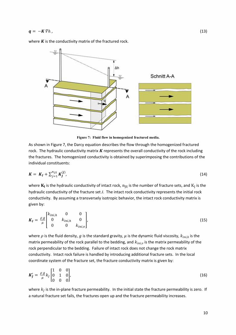
models. It integrates subsurface characteristics, well, completion, operation, diagnostic, and well
performance analysis. Using asset specific data, it is able to develop an optimal completion design
with a set of prioritized completion and operation parameters. This results in reducing the number
of field trials for achieving the optimal completion design. In addition, it provides valuable insights
for further data acquisition to evaluate and forecast well performance.
Field trials based on the results from this approach have yielded encouraging production uplifts with
quality forecasts. We believe it is technically feasible to derive an optimal completion design using a
subsurface based forward modeling approach that will deliver significant value to the industry.
Introduction Unconventional reservoirs produce substantial quantities of oil and gas. These reservoirs are usually
characterized by ultra-low matrix permeability. Most unconventional reservoirs are hydraulically
fractured in order to establish more effective flow from the reservoir and fracture networks to the
wellbores. The success of hydraulic fracture stimulation in horizontal wells has the potential to
dramatically change the oil and gas production landscape across the globe and the impacts will
endure for decades to come.
For a given field development project, the economics are highly dependent completion establishing
effective and retained contact with the hydrocarbon bearing rocks. Well and completion design
parameters that influence the economic success of the field development include well orientation
and landing zone, stage spacing and perforation cluster spacing, fluid volume, viscosity and pumping
rate, and proppant volume, size and ramping schedule. Optimization of these design parameters to
maximize asset economic value is key to the success of every unconventional asset.
2
To achieve an optimal completion design for an asset, the current industry practice is to conduct a
large number of field trials that require high capital investment and long cycle-time, and most
importantly, significantly erode the project value. The workflow and toolkits shown in this paper are
based on the Dynardo technology (Dynardo GmbH 2013) that offer a much cheaper and faster
alternative approach in which to develop an optimal well completion design for EUR and unit
development cost (UDC) improvements. It provides an integrated well placement and completion
design optimization process that integrates geomechanics descriptions, formation characterizations,
In the simulation, the loading conditions are applied either to the well pipe or to the perforation
pipe. Two types of loading conditions are supported, i.e., flux and pressure.
A flux loading condition is defined by prescribing pumping rate. By applying the pumping rate to the
well pipe, as shown in Figure 10, we mimic flow distribution among the perforations as in actual frac
jobs. In other words, the flow through a perforation into the formation is determined by the
resistance of fracture propagation at that perforation location.
Alternatively, a pressure loading condition can be applied by prescribing bottom-hole pressure (BHP).
In this case, the measured or calculated BHP pressure is applied directly to the perforation pipe.
Figure 11 shows that BHP is prescribed at the nodes at the intersections between perforation pipes
and well pipe.
Model Calibration After model construction, calibration of large amounts of uncertain parameters to the best available
measurements is conducted. A parameter identification problem exists simply because of the large
number (>100) of model parameters, and they may have a considerable associated uncertainly.
During the calibration phase, Dynardo applies optiSLang [4], the Dynardo software for variation and
optimization analysis. The process involves running a set of calibration models with respect to the
variation space of the model. With optiSLang, important parameters in the parametric hydraulic
fracture model can be identified and successively updated for successive model runs, are initialized
and executed in an automated process. With that procedure a large number of calibration
sensitivity design runs can be executed in a relatively short period of time.
The calibration phase ideally requires quality diagnostic data. This includes surface pressure, bottom
hole pressure, and pumping rate histories from diagnostic fracture injection testing (DFIT), which are
used to derive instantaneous shut-in pressure (ISIP), and the pressure and pumping rate histories
and the total slurry volume (fluid plus proppant) for each stage of the actual frac job. The
representative microseismic event catalog is also used in the calibration phase. With optiSLang
reservoir uncertainties are integrated in the calibration process to better identify the most
influential parameters controlling fracture geometry. Thus, model calibration process also provides
insights for additional data gathering to focus on parameters that significantly affect the simulation
results. The details of the calibrations are explained below.
Prescribed BHP on Perforations
16
Calibrating of Fracture Initiation and Termination Conditions
After model initialization with in-situ stress field and initial pressure conditions, the pressures at
which hydraulic fractures initiation and termination are verified. ISIP from DFIT is used to define
fracture initiation and fracture extension. Uncertainty of ISIP is estimated with minimum, mean, and
maximum values. Typical adjustments during calibration to ISIP conditions include formation
pressure and in-situ stress conditions within and nearby the perforated layers, and strengths of the
natural fractures within and nearby the perforated layers.
Calibrations with Bottom Hole Pressure and Pumping Rate
By applying the actual pumping rate, we calculate the BHP (bottom hole pressure) response and
compare with the measured BHP (or projected BHP from the surface pressure) based on data from
the actual frac job. Conversely, by applying the BHP from the frac job, we calculate the flow rate
through the perforations into the formation and compare the calculated value with the measured
pumping rate. The major parameters calibrated in this step are strengths of intact rocks, activated
mean spacings and strengths of the natural fractures in the different layers, maximum hydraulic
opening of the activated fractures, and overall energy loss due to friction, leak off, turbulent flow or
other dissipate mechanisms that are summed up into the specific storativity of the Darcy flow
equation.
Calibration of Generated Fracture Volume with Pumped Total Fluid
Volume
The generated fracture volume is compared with the pumped total fluid volume in the rate and
pressure calibration introduced above. The generated total fracture volume is calculated based on
mechanical openings of the fracture. As the permeability of unconventional rocks is low in general,
and assuming very low fluid leak off during fracing, the total fracture volume should be close to the
pumped total fluid volume. Since proppant placement is not explicitly modeled in the current
approach, we count the proppant volume into the total fluid volume in this calibration.
Calibration of Computed SRV with Microseismic Data
Microseismic data provides the time, the position (point), and the magnitude of each individual
microseismic event, which is believed to represent shear failure of reservoir rocks during hydraulic
fracturing. The “dot-plot” of microseismic events is used as a representation of the spatial extension
of hydraulic fractures. For model calibration with microseismic data, the “dot-plot” is compared to
the simulated rock failure. In this context, two different methods are applied. In the first method,
the microseismic events and calculated stimulated rock volume (SRV) represented by the collection
of all failed elements are plotted together at different time steps. This allowed a visual comparison
of spatial distribution of both of the data sets. The check point in this calibration is to see whether
the SRV extensions from the model fit the overall hydraulic fracture length and height indicated by
the microseismic data in the horizontal and vertical directions, respectively. The drawback of this
method is that it is very challenging to define a clear objective measure for the quality of the fit,
which is needed for in the automatic calibration procedure.
In the second method, the mechanically failed elements are considered as “cracking” events. If the
calculated fracture opening in a failed element exceeds a certain threshold, the time step and the
17
location of the element center point is stored. The distance between the center of the cracked
element to the stage center is calculated. The calibration is to compare the distance with the
distance between the microseismic event and the stage center.
Optimization of Well and Completion Designs Once the model is calibrated with all the procedures described in the previous section, it is then
used in forecast mode to optimize well and completion designs. The optimization involves two
critical procedures, i.e., defining the objective function for optimization and defining the parametric
space. Parametric modeling is conducted with respect to two parametric spaces. First is the
subsurface parametric space, which represents the reservoir uncertainties and gives the ranking of
subsurface parameters based on their impacts to the objective function. It provides insights to
future data acquisition programs. The second are the well and completion parameters, which yield
the optimized well and completion design corresponding to the objective function.
Most of the subsurface parameters are defined for each individual layer and for each natural
fracture set in the model. Together with the well and completion parameters, it is common that
several hundred parameters are defined. To handle this large amount of parameters and their
uncertainties, the Dynardo technology utilizes optiSlang, which performs a few procedures including
searching the whole uncertainty space defined by the uncertainty ranges of all the parameters as
well as experimental design scenarios, generating ANSYS input files corresponding to the generated
scenarios, launching ANSYS simulations with the input files, taking ANSYS analysis results from the
simulations and saving the results in a database. After a certain sample set is completed optiSLang
search for subspaces of important parameters and generates mapping functions between inputs and
simulation result variations in the so called the metamodel. The metamodels are checked for their
forecast quality based on their responses to input variations. After the forecast quality reaches
certain levels such as 90% the sampling stops. The metamodels provide insights about the ranking
of the parameters based on their impacts to the objective functions defined in the study.
Objective Functions
An objective function is defined based on the specific business driver for an asset. There are a few
potential objective functions, including, but not limited to, total stimulated rock volume (TSRV),
valuable SRV (VSRV), total drainage volume (TDV), accessible hydrocarbon initially in place (AHCIIP),
EUR, and UDC.
TSRV is the total volume of all the mechanically failed elements in the model. It is a gross measure
of the effectiveness of the fracture stimulation. Only a fraction of TSRV contributes significantly to
production. To address the importance of SRV to production, two concepts are proposed,
connected-water-accepting volume (CWAV) and connected-proppant-accepting volume (CPAV).
Based on the mechanical fracture openings, elements are identified as water-accepting or as
proppant-accepting. An element is called a water-accepting element if the mechanical opening of at
least one fracture set in the element exceeds a predefined threshold. Usually a threshold of 0.1 mm
is applied. A proppant-accepting element is identified if the mechanical opening of at least one
fracture set exceeds a multiple of the average proppant size. In most of the Dynardo simulations, a
threshold of three times the average proppant size is applied.
18
In addition to the water-accepting and proppant-accepting elements, their connectivity to the
perforations is identified. An element is connected-water-accepting element if the fluid can flow
from any perforation directly into that element or through other water-accepting elements. The
same principle is applied with to the definition of connected-proppant-accepting elements. The
total volume of all connected-water-accepting elements is called the connected-water-accepting
volume (CWAV). Similarly, the connected-proppant-accepting volume (CPAV) is defined.
The CWAV and CPAV are continuously updated during the simulation. At the beginning of the
simulation, only the perforation elements are considered in the CWAV and CPAV. After every
mechanical step, the water-accepting and proppant-accepting elements and their connectivity status
are updated. Based on the connectivity status from the previous step, the neighbouring water-
accepting or proppant-accepting elements are selected and added to the corresponding CWAV or
CPAV. Two elements are neighbouring elements if they share at least one node. This selection
algorithm is continued until no new neighbour elements are found.
For CPAV, successful proppant placement is assumed. Proppant effects are captured in the fracture
conductivity decline function. The stress dependent fracture conductivity decline with proppant is
only used for the CPAV. Otherwise the stress dependent conductivity decline without proppant is
applied even if the fracture opening is greater than the proppant-accepting opening threshold.
It is observed that only the CPAV is valuable to the production, especially in relatively soft rocks.
Therefore, CPAV is equivalent to VSRV. VSRV is defined as total volume of elements with fracture
opening greater than three times of predefined proppant size and with connection, direct or indirect
through other proppant-accepting elements, to at least one perforation cluster.
TDV is defined as the total volume of all elements that can be drained during the production time of
the well through the VSRV. The VSRV is part of the drainage volume by this definition. An element
outside of the VSRV in the drainage volume is based on the criteria that the element is in the same
element layer of the layered reservoir with at least one connected-proppant-accepting element, and
the distance between the element center and the center of the nearest proppant-accepting element
is less than the drainage distance, which is given by an empirical relation in the form of:
𝑅 [𝑓𝑡] = 𝐶√𝑘𝑖𝑛𝑖,ℎ [𝑛𝐷], (29)
where C is a constant, 𝑘𝑖𝑛𝑖,ℎ is the matrix horizontal permeability of the rocks in the layer.
The criteria are defined with consideration of the permeability anisotropy of unconventional rocks,
i.e., the horizontal permeability of the rocks is usually several orders of magnitude larger than the
vertical permeability due to layering and the laminated natural of unconventional rocks.
ACHIIP is estimated based on TDV and hydrocarbon content, which can be calculated with:
𝐴𝐻𝐶𝐼𝐼𝑃 = ∑ 𝑉𝑑𝑟𝑎𝑖𝑛,𝑖 ⋅ 𝑉𝑔,𝑠𝑓𝑐,𝑖𝑛𝐿𝑖=1 , (30)
where 𝑛𝐿 is the number of layers, 𝑉𝑑𝑟𝑎𝑖𝑛,𝑖 is the drainage volume of the i-th layer and 𝑉𝑔,𝑠𝑓𝑐,𝑖 [v/vbulk] is
the volume of hydrocarbon at surface conditions stored in one cubic foot of formation in the ith
layer.
19
The AHCIIP can be calculated after every stage of stimulation. To provide estimate of AHCIIP for the whole well with the commonly used three-stage model, we differentiate the first stage from the other stages with consideration of stress shadow effects to the second and third stages but not the first (virgin) stage. Therefore, the accessible hydrocarbon initially in place for the whole well (AHCIIPWell) is calculated as:
𝐴𝐻𝐶𝐼𝐼𝑃𝑊𝑒𝑙𝑙 =𝐴𝐻𝐶𝐼𝐼𝑃𝑠𝑡𝑎𝑔𝑒3−𝐴𝐻𝐶𝐼𝐼𝑃𝑠𝑡𝑎𝑔𝑒1
2⋅ (
𝑙𝑤𝑒𝑙𝑙,𝑡𝑜𝑡
Δ𝑆𝑡𝑎𝑔𝑒+𝑙𝑆𝑡𝑎𝑔𝑒− 1) + 𝐴𝐻𝐶𝐼𝐼𝑃𝑠𝑡𝑎𝑔𝑒1 , (31)
where 𝑙𝑤𝑒𝑙𝑙,𝑡𝑜𝑡 is the total horizontal well length, Δ𝑆𝑡𝑎𝑔𝑒 is the stage spacing and 𝑙𝑆𝑡𝑎𝑔𝑒 is the stage
length. Note that AHCIIPstage1 and AHCIIPstage3 are the AHCIIP after Stages 1 and 3 are stimulated. Please note repeatable performance for all stages after Stage 1 is assumed.
Well EUR can be calculated based on AHCIIPWell by assuming a recovery factor. This method fits for
assets with limited production data, i.e., appraisal phases. For assets with reasonable amounts of
production data, it is recommended to use another approach for EUR calculation. This approach
relies on correlating EUR, from production data analysis, such as decline curve analysis, with one of
the objective variables from Dynardo simulation, such as TSRV, VSRV, TDV, or AHCIIP. With this
correlation, EUR’s of wells with different completion designs can be predicted. The two EUR
prediction methods can be used to cross check each other for assets with enough production data.
UDC prediction can be made using the predicted EUR from a specific completion design and the cost
of that completion based on the actual service contracts of the asset.
Sensitivity Study, Parametric Ranking, Meta Model Generation and
Optimization
Subsurface parameters are input to the model either as boundary conditions or initial conditions.
These parameters have great influences to the objective functions. The impacts of the subsurface
parameters on the objective functions depend on their uncertainty ranges as well as their driving
mechanisms to hydraulic fracturing. The ranking of the parameters shows which parameter or
group of parameters should be focused on in reducing their uncertainties, and thus, provides insight
on future data acquisition programs.
The well and completion parameters include well orientation, landing zone, stage and perforation
parameters, fluid volume, pumping rate, and fluid viscosity. The current version of the technology
does not handle proppant transport, which will be a major update in the upcoming version. The
sensitivity study presents a set of well and completion design parameters that define the optimal
design to achieve the specific objective defined by the objective function. It also provides the
ranking of the well and completion design parameters based on their impacts to the objective
functions.
The sensitive study is automatically driven by optiSLang. The optiSLang module searches the
uncertainty space defined by the uncertainty ranges of the subsurface as well as well and
completion parameters. It comes up with experimental design scenarios, generates ANSYS input
files corresponding to the scenarios, launches ANSYS simulations with the input files, takes ANSYS
analysis results from the simulations, and saves the scenarios and results in the metamodel. The
resulting metamodel is used to rank the input parameters based on their impacts to the objective
functions. The ranking is based by the coefficient of prognosis (CoP), which is defined as:
𝐶𝑜𝑃 = 1 −𝑆𝑆𝐸
𝑃𝑟𝑒𝑑𝑖𝑐𝑡𝑖𝑜𝑛
𝑆𝑆𝑇, (32)
20
where 𝑆𝑆𝐸𝑃𝑟𝑒𝑑𝑖𝑐𝑡𝑖𝑜𝑛 is the sum of squared prediction error, 𝑆𝑆𝑇is the total variation.
Upon finishing the sensitivity study the metamodels are available inside optiSLang or in Excel. The
metamodel provides the opportunity to quickly check scenarios other than that already investigated
in the sensitivity study and optimization process. For example, if the optimum completion design
from the model showed two clusters were the best cluster design to maximize EUR, one could ask
how much EUR reduction would it incur if three or four clusters were used? The metamodel quickly
renders an answer. The metamodel also provides the opportunity to handle subsurface parameter
changes across different areas of an asset, new well and completion designs, and even changing key
business drivers, without building a new model as long as the initial variation windows of reservoir
uncertainties and operational parameter covers the design values to be analyzed.
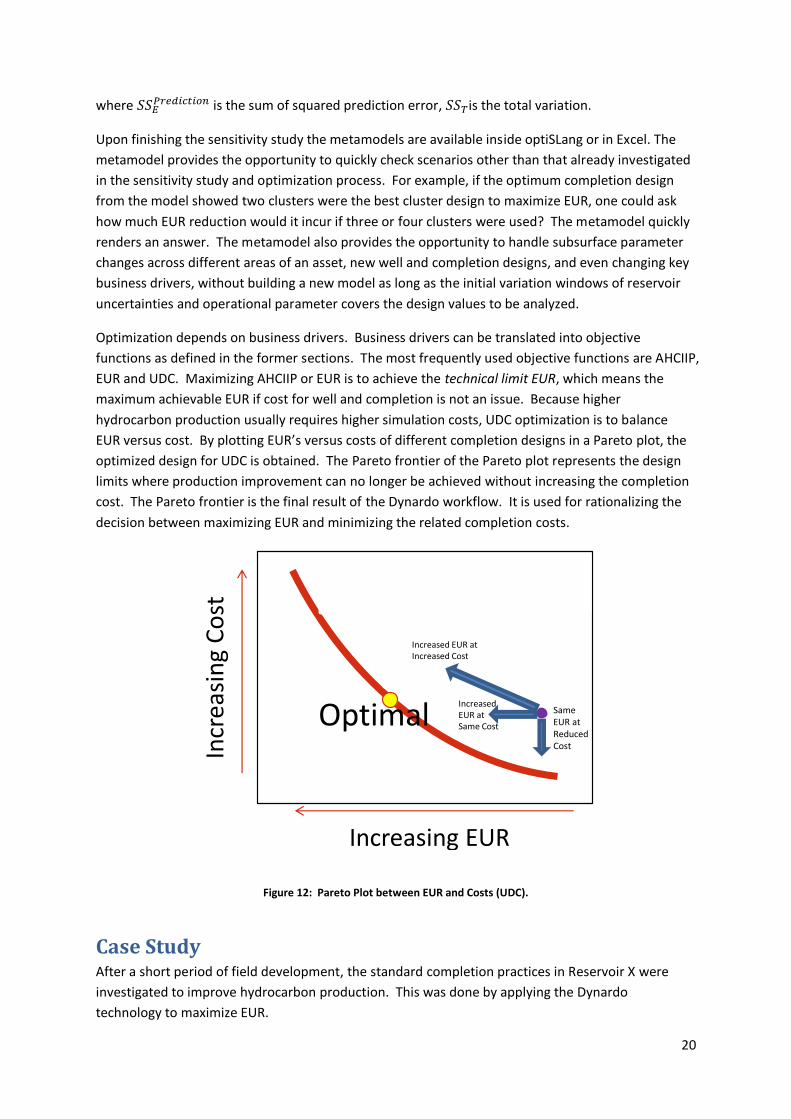
Optimization depends on business drivers. Business drivers can be translated into objective
functions as defined in the former sections. The most frequently used objective functions are AHCIIP,
EUR and UDC. Maximizing AHCIIP or EUR is to achieve the technical limit EUR, which means the
maximum achievable EUR if cost for well and completion is not an issue. Because higher
hydrocarbon production usually requires higher simulation costs, UDC optimization is to balance
EUR versus cost. By plotting EUR’s versus costs of different completion designs in a Pareto plot, the
optimized design for UDC is obtained. The Pareto frontier of the Pareto plot represents the design
limits where production improvement can no longer be achieved without increasing the completion
cost. The Pareto frontier is the final result of the Dynardo workflow. It is used for rationalizing the
decision between maximizing EUR and minimizing the related completion costs.
Figure 12: Pareto Plot between EUR and Costs (UDC).
Case Study After a short period of field development, the standard completion practices in Reservoir X were
investigated to improve hydrocarbon production. This was done by applying the Dynardo
technology to maximize EUR.
Increasing Cost
Incr
easin
gEU
R
UDC Optimization – Balance EUR & Cost
– Operation Standardization & Optimization
Incr
easi
ng
Co
st
Increasing EUR
Same EUR at Reduced Cost
Increased EUR at Same Cost
Increased EUR atIncreased Cost
Optimal Same EUR at Reduced Cost
21
Model Construction, Initialization and Calibration Figure 12 shows the map view of a well pad in Reservoir X. Well 3-H was chosen as the well to
model. It was the first well completed on the pad. Stages 6, 7, and 8 were chosen for the model
primarily because of the high quality of microseismic data, which was acquired from a nearby
vertical monitoring well, Well 1-V. Also, Stages 6, 7, and 8 were not affected by any faults that might
add uncertainties to the modeling results.
Layering of the model was defined based on core and log data derived mechanical properties,
lithology types, rock structures and textures, permeability, porosity and hydrocarbon saturation.
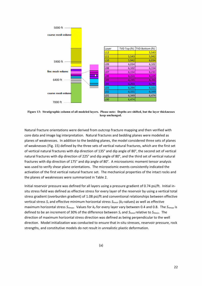
Thirteen layers were defined in the model (Figure 13). All the three stages were landed in rock layer
L04. Based on the layering and geometric measurements of the stages, FEM meshes were
constructed as shown in Figure 14.
Figure 12: Well Location Map.
22
Figure 13: Stratigraphic column of all modeled layers. Please note: Depths are shifted, but the layer thicknesses keep unchanged.
Natural fracture orientations were derived from outcrop fracture mapping and then verified with
core data and image log interpretation. Natural fractures and bedding planes were modeled as
planes of weaknesses. In addition to the bedding planes, the model considered three sets of planes
of weaknesses (Fig. 15) defined by the three sets of vertical natural fractures, which are the first set
of vertical natural fractures with dip direction of 135° and dip angle of 80°, the second set of vertical
natural fractures with dip direction of 225° and dip angle of 80°, and the third set of vertical natural
fractures with dip direction of 175° and dip angle of 80°. A microseismic moment tensor analysis
was used to verify shear plane orientations. The microseismic events consistently indicated the
activation of the first vertical natural fracture set. The mechanical properties of the intact rocks and
the planes of weaknesses were summarized in Table 2.
Initial reservoir pressure was defined for all layers using a pressure gradient of 0.74 psi/ft. Initial in-
situ stress field was defined as effective stress for every layer of the reservoir by using a vertical total
stress gradient (overburden gradient) of 1.08 psi/ft and conventional relationships between effective
vertical stress Sz and effective minimum horizontal stress Shmin (k0-values) as well as effective
maximum horizontal stress SHmax. Values for k0 for every layer vary between 0.4 and 0.8. The SHmax is
defined to be an increment of 30% of the difference between Sz and Shmin relative to SHmin. The
direction of maximum horizontal stress direction was defined as being perpendicular to the well
direction. Model initialization was conducted to ensure that in-situ stresses, reservoir pressure, rock
strengths, and constitutive models do not result in unrealistic plastic deformation.
(a)
5000 ft
5900 ft
6400 ft
7000 ft
Layer TVD Top (ft) TVD Bottom (ft)
L12 5,543
L11 5,543 5,942
L10 5,942 6,034
L09 6,034 6,102
L08 6,102 6,154
L07 6,154 6,231
L06 6,231 6,245
L05 6,245 6,261
L04 6,261 6,294
L03 6,294 6,331
L02 6,331 6,349
L01 6,349 6,474
L00 6,474
23
(b)
Figure 14: FEM Meshes. (a). FE-Model with stage 6,7,8 and perforations in layer L04. (b). Mesh for hydraulic analysis
Figure 15: Orientations of the planes of weaknesses considered in the model.
Table 2: Mechanical properties of intact rocks and planes of weaknesses.
20.44 25 5 no vertical joints no vertical joints no vertiacljoints
L07 17,367 45 3,597 10%
20.44 25 5 20.44 25 5 20.44 125 25 20.44 125 25
L06 16,505 45 3,418 10%
20.44 25 5 20.44 25 5 20.44 125 25 20.44 125 25
L05 16,260 45 3,368 10%
20.44 25 5 20.44 25 5 20.44 125 25 20.44 125 25
L04 15,428 45 3,195 10%
20.44 25 5 20.44 25 5 20.44 125 25 20.44 125 25
L03 9,917 45 2,054 10%
20.44 25 5 20.44 25 5 20.44 125 25 20.44 125 25
L02 11,189 45 2,317 10%
20.44 25 5 20.44 25 5 20.44 125 25 20.44 125 25
L01 29,919 45 6,196 10%
20.44 25 5 no vertical joints no vertical joints no vertical joints
L00 15,145 Elastic
Elastic
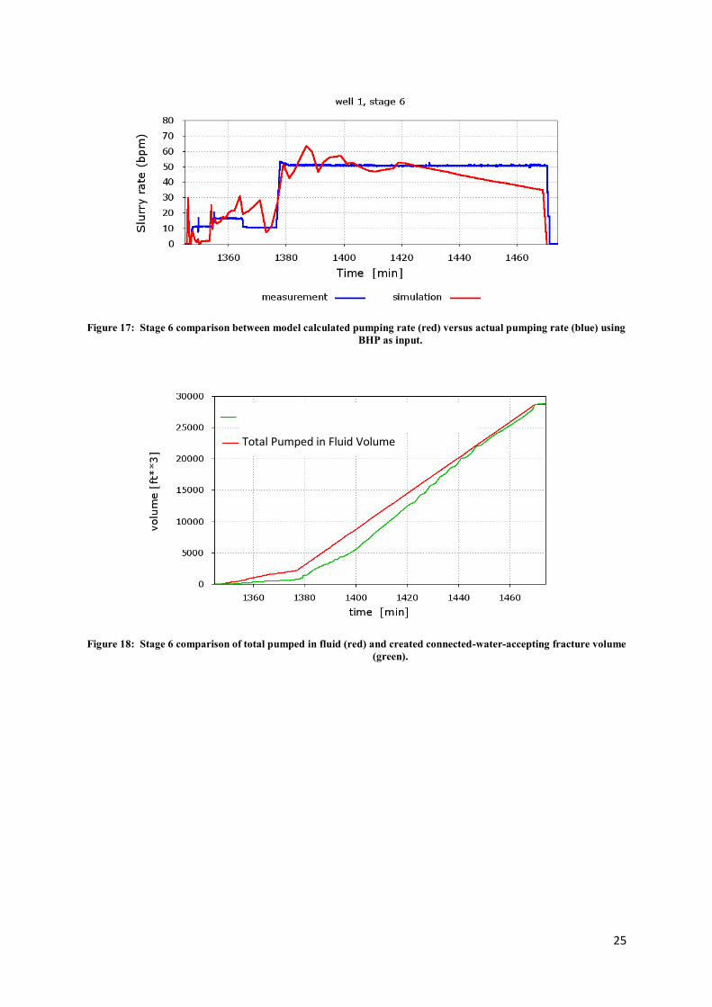
Model calibration was conducted by matching the fracture initiation and termination behaviors from
the DFIT data, by matching bottom hole pressure response using pumping rate as input (Fig. 16), and
vice versa (Fig. 17), by matching the generated fracture volume with the pumped total fluid volume
(Fig. 18), and by matching the plastically deformed rocks from the model with the microseismic
distributions (Fig. 19).
Figure 16: Stage 6 comparison between model calculated BHP (red) versus actual BHP (blue) using pumping rate as input.
25
Figure 17: Stage 6 comparison between model calculated pumping rate (red) versus actual pumping rate (blue) using BHP as input.
Figure 18: Stage 6 comparison of total pumped in fluid (red) and created connected-water-accepting fracture volume (green).
Total Pumped in Fluid Volume
Connected-Water-Accepting Fracture Volume
26
Figure 19: Plot of connected proppant-accepting elements and microseismic events at the end of Stage 6.
Sensitivity Study and Results The calibrated model was then used to run sensitivity analyses with respect to well and completion
design parameters including well landing depth, stage parameters (stage spacing, number of
clusters), pumping parameters (pumping rate and volume), and fluid viscosity. The defined
uncertainty windows of the parameters are summarized in Table 3. The number of perforations and
the well landing depth were defined as discrete parameters. All other parameters continuously
varied between the lower and upper bounds. In order to modify pumping rate and total pumped
volume using a parametric procedure, the pumping rate function was idealized to be identical for
every stage and having identical waiting time between stages.
The objective function was defined as VSRV. To come up with the optimal design with maximized
VSRV, the metamodel derived from the sensitivity analysis was used. The optimized design is
summarized in Table 3. With the optimized design, potentially doubling of the VSRV was indicated.
Table 3: Well and completion parameters of base design and optimal design and their uncertainty ranges.
Parameter Reference Design Uncertainty Range Optimal Design
Landing Zone (ft) L04 L02 – L08 L05
Perforation Clusters per Stage 4 1 – 5 1
Stage Spacing (ft) 300 150 – 650 250
Pumping Rate (bpm) 50 30 – 100 100
Total Fluid Volume (bbls) 4500 4000 – 8000 7800
3D View Map View
Cross Section View – Perpendicular to Well Cross Section View – Parallel to the Well
27
Verification of Model Prediction with Data from Neighboring Wells The performance of unconventional wells, to a large extent, depends on geology. However,
completion is also critical to the success of unconventionals. Because of the large number of
uncertain parameters in the process, it is costly to conduct field pilots to understand the impacts of
all the parameters. What is proposed here is a physics or model guided approach that enables us to
better use available well performance data compared to the commonly applied multi-variant
analysis. It reduces the number of field trials needed to come up with optimal completion designs.
To verify the model prediction, we used well completion and performance data of neighboring wells
to ensure the wells we compared with were in similar geological settings. The wells were located up
to 10,000 feet from the center of the well pad shown in Fig. 12. The EUR numbers were from
pressure decline analysis with six months and more production history. The VSRV numbers were
from the metamodel built in this study and based on the actual completion parameters of the wells.
The EUR’s versus VSRV’s are plotted in Fig. 21. The plot shows a clear trend of completion impact to
well performance. The best fit curve shows a slightly non-liner correlation between EUR and VSRV.
It is worth mentioning that the plot was made after the metamodel was built, which means it was a
blind prediction.
Figure 20: Plot of decline curve analysis (DCA) derived EUR versus Dynardo predicted VSRV values.
Field trials were also conducted to verify the optimal completion design on a five-well pad. Within
the five wells, one well was completed with the recommended optimal design based on this work.
The other wells were completed with the base completion design of the asset. Early preduction
showed more than 20% uplift in production from the well completed with the optimal design
compared to the other four wells. Details of the field trials will be explained in another paper.
Summary The Dynardo technology provides a subsurface based completion optimization toolkit that integrates
subsurface, well, completion, production, diagnosis, and cost data for well and asset value delivery.
Optimal
VSRV from Dynardo Simulation
EUR
fro
m D
CA
An
alys
is
28
Compared to common practice, i.e., field trials, the technology offers a much cheaper and faster
alternative approach to develop an optimal well completion design for EUR and UDC improvement.
Application of the technology clearly showed its predictability. Field trials based on the optimal
completion design from Dynardo modeling showed encouraging production uplift. We are
convinced that it is feasible to derive an optimal completion design using a subsurface based
forward modeling approach that will deliver significant value to the industry.
Acknowledgement The authors would like to thank Shell Oil Company, especially Bill Westwood, Sam Whitney, Shawn
Holzhauser, Simon James, and Lee Stockwell for their continuously supports for Dynardo technology
development, case studies and field trials in the past five years. Special thanks to the assets teams in
USA, Canada, China, and Argentina for their interests in the technology and for their support for the
asset specific studies. Also, thanks to Shawn Holzhauser and Brent Williams for their detailed review
of this paper, and to Anna Yankow for editing this paper.
References Gangi, A. F. (1978). Variation of whole and fractured porous rock permeability with confining
pressure. International Journal of Rock Mechanics and Mining Sciences & Geomechanics Abstracts, 15(5), 249-257.
ANSYS, Inc. . (2013). ANSYS ® , Release 14.5 . Canonsburg, PA. Barton, N., Bandis, S., & Bakhtar, K. (1985, June). Strength, deformation and conductivity coupling
of rock joints. International Journal of Rock Mechanics and Mining Sciences & Geomechanics Abstracts, 22(3), 121–140.
Bathe, K. J. (1985). Finite element procedures. Prentice Hall. Dynardo GmbH. (2013). 3D Hydraulic fracturing simulator, version 3.7.4, documentation.ppt .
Weimar. Dynardo GmbH. (2013). multiPlas – elastoplastic material models for ANSYS, Version 5.0.593.
Weimar. Dynardo GmbH. (2013). optiSLang ® - The optimizing Structural Language, Version 4.1.0 . Weimar. Iragorre, M. T. (2010). Thermo-hydro-mechanical analysis of joints a theoretical and experimental
study. Barcelona: Phd-Thesis, Univesitat politècnica de Catalunya. Jirasek, M., & Bazant, Z. P. (2001). Inelastic Analysis of Structures. John Wiley & Sons. Most, T., & Will, J. (2012). Efficient sensitivity analysis for virtual prototyping. Proceedings of the
6th European Congress on Computational Methods in Applied Sciences and Engineering. Vienna.
Pölling, R. (2000). Eine praxisnahe, schädigungsorientierte Materialbeschreibung von Stahlbeton für Strukturanalysen. Dissertation, Ruhr-Universität Bochum.
Simo, J. C., & Hughes, T. J. (1998). Computational Inelasticity. Springer. Weijers, L. (October 2007). Evaluation of Oil Industry Stimulation Practices for Engineered
Geothermal Systems, Pinnacle Report DOE-PS36-04GO94001. Will, J. (1999). Beitrag zur Standsicherheitsberechnung im geklüfteten Fels in der Kontinuums- und
Diskontinuumsmechanik unter Verwendung impliziter und expliziter Berechnungsstrategien. In Berichte des Institutes für Strukturmechanik 2/99. Dissertation, Bauhaus Universität Weimar.
29
Will, J., & Schlegel, R. (2010). Simulation of hydraulic fracturing of jointed rock. Proceedings of European Conference on Fracture. Dresden.
Wittke, W. (1984). Felsmechanik: Grundlagen für wirtschaftliches Bauen im Fels. Springer-Verlag.