Young Flattenings in the Schur module basis

Lennart J. Haas and Christian Ikenmeyer

April 2021

Abstract

There are several isomorphic constructions for the irreducible polynomial representations of the generallinear group in characteristic zero. The two most well-known versions are called Schur modules and Weylmodules. Steven Sam used a Weyl module implementation in 2009 for his Macaulay2 package PieriMaps.This implementation can be used to compute so-called Young flattenings of polynomials. Over the Schurmodule basis Oeding and Farnsworth describe a simple combinatorial procedure that is supposed to give theYoung flattening, but their construction is not equivariant. In this paper we clarify this issue, present thefull details of the theory of Young flattenings in the Schur module basis, and give a software implementationin this basis. Using Reuven Hodges’ recently discovered Young tableau straightening algorithm in the Schurmodule basis as a subroutine, our implementation outperforms Sam’s PieriMaps implementation by severalorders of magnitude on many examples, in particular for powers of linear forms, which is the case of highestinterest for proving border Waring rank lower bounds.

Keywords: Young flattening, representation theory, Pieri’s rule, border Waring rank, complexity lower bounds

AMS Subject Classification 2020: 05E10, 68Q17

ACM Subject Classification: Mathematics of computing → Mathematical software

Computing methodologies → Symbolic and algebraic manipulation → Computer algebra systems

Theory of computation → Computational complexity and cryptography → Algebraic complexity theory

1 Motivation

Young flattenings of polynomials are equivariant linear maps from a space of homogeneous poly-nomials to a space of matrices, where the row and column space are irreducible representationsof GLn := GL(Cn). One is usually interested in finding lower bounds for the rank of the imageof a Young flattening, as it can be used to obtain lower bounds on the border Waring rank of apolynomial, and more generally for any border X-rank for a GLn-variety X, i.e., given a pointp to find a lower bound on the smallest i such that p lies on the i-th secant variety of X, seee.g. [Lan15]. One early example are Sylvester’s catalecticants [Syl52]. Landsberg and Ottaviani[LO15] use Young flattenings in the tensor setting. The name Young flattening was introducedin the predecessor paper [LO13]. Young flattenings also appear in disguise in the area of alge-braic complexity theory as matrices of partial derivatives, shifted partial derivatives, evaluationdimension, and coefficient dimension [NW95, GKKS14]. They can in principle be used to findcomputational complexity lower bounds in many algebraic computational models such as borderdeterminantal complexity (see [LMR13]) and border continuantal complexity [BIZ18], which makesYoung flattenings an interesting tool in the Geometric Complexity Theory approach by Mulmuleyand Sohoni [MS02], [MS08], [BLMW11]. Limits of these methods (in the case of studying X-rank)have recently been proved in [EGOW18, GMOW19]. No such limits are known for using Youngflattenings to study the orbit closure containment problems in geometric complexity theory. Firstresults in this direction were obtained in [ELSW18], where limits to the method of shifted partialderivatives are shown. This was improved on in [GL19], where a setting was given in which Youngflattenings give strictly more separation information than partial derivatives.

The Waring rank of a homogeneous degree d polynomial p ∈ SdV is defined as the smallest rsuch that p can be written as a sum of r many d-th powers of homogeneous linear forms (arbitrarylinear combinations of d-th powers are usually allowed if the base field is not algebraically closed).

1

arX

iv:2

104.

0236

3v1

[m

ath.

AG

] 6

Apr

202

1

2 Preliminaries 2

For example (x− y)3 + y3 = x3− 3x2y+ 3xy2, hence x3− 3x2y+ 3xy2 has Waring rank at most 2.The border Waring rank of p is the smallest r such that p can be approximated arbitrarily closelycoefficient-wise by polynomials of Waring rank at most r. For example 3εx2y = limε→0((x+εy)3−x3), hence x2y has border Waring rank at most 2.

If a Young diagram λ is contained in another Young diagram µ such that the column lengthsof both diagrams differ by at most 1 in each column, then we have a unique nonzero equivariantmap between SdV ⊗ SλV → SµV, where SλV , SµV , and SdV are irreducible polnomial GLn-representations, and d is the difference in the number of boxes of µ and λ. This is called the Pierimap, and it induces a linear map Fλ,µ : SdV → End(SλV,SµV ). Since border Waring rank issubadditive, a lower bound on the border Waring rank of p is obtained by rounding up to quotientof ranks ⌈

rank(Fλ,µ(p))

rank(Fλ,µ(xd))

⌉, (1.1)

where x is some variable that appears in p, and rank(.) is the usual rank of matrices.There are several isomorphic constructions for the irreducible polynomial representations of

the general linear group in characteristic zero. The two best known versions are called Schurmodules and Weyl modules and they only differ in the order of the row-symmetrizer and thecolumn-symmetrizer in their definition of the Young symmetrizer. This results in different basesfor the irreducible representations. Sometimes results that are proved in one basis are reproved inthe other basis, but the proofs look significantly different (see e.g. [BCI11] and [MM14]). In fact,so far some results are only provable in a natural way over one basis and not the other, see e.g.[Res20]. Based on an explicit paper by Olver over the Weyl module basis [Olv82] Steven Sam in2009 implemented his Macaulay2 package PieriMaps [Sam08], which among other things can beused to compute the rank quotient (1.1), see Section 4 (A) below.

The papers [Far16] (in its Section 51) and [Oed16] (only in version 1) describe the PieriMapspackage as if it would be working in the Schur module basis and they assume that the Youngflattenings have an extremly simple combinatorial description. However, this is wrong (see Section 5below), which led to a revision of [Oed16].

In this paper we work out the details of Young flattenings in the Schur module basis: Weclosely mimic the arguments in [Olv82], but we take care of subtle sign issues that are not presentin Olver’s work over the Weyl module basis. We then make use of a recent fast algorithm (andimplementation) by Reuven Hodges for Young tableau straightening in the Schur module basis[Hod17] to get a highly efficient Young flattening algorithm that outperforms Sam’s PieriMapsimplementation by several orders of magnitude in many examples. We obtain the most impressivespeedup factor of 1000 for flattening the power of a linear form, which is the denominator of (1.1).

Our contribution is therefore twofold: We thoroughly clarify the theory of Young flattenings inthe Schur module basis and we present a new and efficient implementation for Young flatteningsthat uses Hodges’ state-of-the-art straightening algorithm over the Schur module basis.

2 Preliminaries

A composition ν of a number d is a finite list of natural numbers adding up to d, i.e., (3, 0, 2, 4)is a composition of 9. A partition is a nonincreasing composition, for example λ = (6, 4, 3) is apartition. We write λ ` d if λ is a partition of d. We write λi = 0 if i is greater than the number ofentries in λ. We define `(λ) := min{i | λi = 0}−1. We identify a partition with its Young diagram,which is a top-left justified array of boxes, i.e., the set of points {(i, j) | 1 ≤ i and 1 ≤ j ≤ λi}.For example, the Young diagram corresponding to (6, 4, 3) is

and we have (2, 4) ∈ λ and (4, 2) /∈ λ. We see that `(λ) is the number of rows of the Young diagramcorresponding to λ. We denote by |λ| the number of boxes in λ, i.e., |λ| =

∑i λi. We denote by λ∗

1 Although the description in the paper is wrong, the use of the software package is correct and gives the resultclaimed in the paper.

2 Preliminaries 3

the Young diagram obtained by reflecting λ at the main diagonal, e.g., (6, 4, 3)∗ = (3, 3, 3, 2, 1, 1).It follows that λ∗i is the length of the i-th column of λ. We write λ ⊆ µ if for all (i, j) ∈ λ we have(i, j) ∈ µ. If λ ⊆ µ, then we denote by µ/λ the set of points that are in µ but not in λ. We callµ/λ a horizontal strip if it has at most 1 box in each column. In this situation we write µ/λ ∈ HS.

A Young diagram λ whose entries are labeled with numbers is called a Young tableau of shape λ.For example,

6 3 4 2 3 33 3 1 26 6 3

is a Young tableau of shape (6, 4, 3). A Young tableau is called semistandard if the entries strictlyincrease in each column from top to bottom and do not decrease in each row from left to right.

For example, 1 1 1 32 3 is a semistandard tableau. We denote by Sλ the symmetric group on the

set {(i, j) | (i, j) ∈ λ} of positions in λ. The group Sλ acts on the set of all Young tableaux ofshape λ by permuting the positions. We write σT for the permuted Young tableau, where λ is theshape of T and σ ∈ Sλ. For a subset S ⊆ λ of positions we write SS to denote the symmetricgroup that permutes only the positions in S among each other and fixes all other positions.

Let V ⊗λ := V ⊗|λ| be the |λ|-th tensor power of a vector space V and associate to every tensorfactor V a position in λ. A rank 1 tensor v = v1⊗v2⊗· · ·⊗v|λ| can now be represented by a Youngdiagram in whose i-th box we write the vector vi. If we fix a basis v1, . . . , vn of V , then a basisof V ⊗λ is obtained by all ways of writing {v1, . . . , vn} into the boxes of λ, allowing repetitions. Ifthe fixed basis is clear from the context, then we write i instead of vi into the boxes and obtain aYoung tableau. The basis vector corresponding to the Young tableau T is also denoted by T whenno confusion can arise, so for example if x = v1 + v2 we can use the multilinearity of the tensorproduct to write

x v2v1

= 1 21 + 2 2

1

2 (A) The Weyl module basis

Let λ be a Young diagram and let (i, j) ∈ λ such that (i + 1, j) ∈ λ (i.e., the box below (i, j) isstill in λ). Then we define Bi,j := {(i, k) | j ≤ k ≤ λi} ∪ {(i + 1, k) | 1 ≤ k ≤ j}. Pictorially,Bi,j(λ) is the subset of the boxes of λ given by collecting all boxes on the following path: Startat position (i+ 1, 1) and move from left to right along row i+ 1 to box (i+ 1, j), then switch therow to (i, j) and move along row i until reaching (i, λi). For example, B1,3((6, 4, 3)) is given bythe dotted boxes in the following diagram:

• • • •• • • .

2.1 Definition (Weyl module, [Wey03, 2.1.15]). The Weyl module Wλ(V ) is defined as thequotient space V ⊗λ/Pλ, where Pλ ⊆ V ⊗λ is the linear subspace generated by the following twotypes of vectors:

1. (Symmetric relation) T − σT , if σ is a permutation that preserves the row indices of allpositions of λ (in other words, σ permutes within the rows of λ).

2. (Shuffle relation)∑σ∈SBi,j(λ)

σT, if i, j ∈ N such that (i, j), (i+ 1, j) ∈ λ.

The Weyl modules for Young diagrams λ with at most dimV rows form a complete list ofpairwise non-isomorphic irreducible polynomial representations of GL(V ). In this paper we willnot work with Weyl modules, but with the isomorphic Schur modules, which are defined in thefollowing section.

2 (B) The Schur module basis

Let T be a Young tableau of shape λ. Let 1 ≤ i < j ≤ λ1 be two column indices. Let B and C betwo equally large sets of boxes, B from column i and C from column j. An exchange tableau of T

2 Preliminaries 4

corresponding to B and C is defined as the tableau arising from T by exchanging the content ofthe boxes B with the content of the boxes C while preserving the vertical order of the entries in Band C. We denote this exchange tableau by EBC (T ). For a subset C of boxes from column j, wewrite EiC(T ) :=

⋃B E

BC (T ), where B ranges over all cardinality |C| subsets of boxes in column i.

2.2 Definition (Schur module). The Schur module SλV is defined as the quotient space V ⊗λ/Qλ

where Qλ ⊆ V ⊗λ is the linear subspace generated by the following vectors

1. (Grassmann relation) T + T ′, where T ′ is obtained from T by swapping two elements in thesame column.

2. (Plucker relation) T−∑T ′∈EiC(T ) for any i and any subset C of a column j 6= i with λ∗i ≥ |C|.

For example, in SλV we have 1 21 4 = 0 and we have 1 2

3 4 = − 3 21 4 by the Grassmann relation.

The Plucker relation gives1 23 4 = 2 1

3 4 + 1 32 4

via E1{(1,2)}. Note that {(1, 2)} is the set containing the single box in row 1 and column 2.

2 (C) The Schur module via moving boxes between columns

If we only consider the Grassmann relation, then we call the quotient Xλ∗V . More formally, letGλ ⊆ V ⊗λ be the linear subspace spanned by the T +T ′, where T ′ is obtained from T by swappingtwo elements in the same column. The quotient V ⊗λ/Gλ is denoted by Xλ∗V . Clearly, in thelanguage of skew-symmetric powers we have

XνV ' (∧ν1V )⊗ · · · ⊗ (

∧ν`(ν)V ). (2.3)

In terms of explicit basees, this isomorphism maps each column from top to bottom to a skew-

symmetric tensor and vice versa: For example, 1 23 4 is mapped to x1 ∧ x3 ⊗ x2 ∧ x4. We define

Yd :=⊕

composition α of d

XαV

as an outer direct sum. Note that each XαV ⊆ V ⊗|α|, but there is no obvious embedding of Yd inV ⊗|α|. In fact, there is a natural isomorphism

Yd '∧d

(V ⊕d) (2.4)

that can be described explicitly in terms of basis vectors using first the isomorphism (2.3): Astandard basis vector

xk1,1 ∧ · · · ∧ xkν1,1 ⊗ xk1,2 ∧ · · · ∧ xkν2,2 ⊗ · · · ⊗ xk1,d ∧ · · · ∧ xkνd,d

is mapped to

xk1,1,1 ∧ · · · ∧ xkν1,1,1 ∧ xk1,2,2 ∧ · · · ∧ xkν2,2,2 ∧ · · · ∧ xk1,d,d ∧ · · · ∧ xkνd,d,d, (2.5)

for example x1 ∧ x3⊗ x2 ∧ x4 is mapped to x1,1 ∧ x3,1 ∧ x2,2 ∧ x4,2. We have an action of GL(V ⊕d)

on∧d

(V ⊕d), which induces an action of GL(V ) via the group homomorphism g 7→ idd ⊗ g, i.e.,sending matrices g to block diagonal matrices that have d many copies of g on their main diagonal.With this action of GL(V ), the isomorphism in (2.4) is an isomorphism of GL(V )-representations.

For given i, j, i 6= j, we consider the Lie algebra element gi,j ∈ gl(V ⊗d) that is a block matrixas follows: the block matrix is zero everywhere but the block (i, j) is the identity matrix on V .Clearly applying gi,j is a GL(V )-equivariant map. Acting with gi,j on the tensor from (2.5) gives∑1≤a≤νi

xk1,1,1∧· · ·∧xkν1,1,1∧· · ·∧xk1,i,[i=a,j,i]∧· · ·∧xkνi,i,[i=a,j,i]∧· · ·∧xkd,1,d∧· · ·∧xkνd,d,d, (2.6)

3 Young Flattenings in the Schur module basis 5

where

[i=a, j, i] :=

{j if i = a

i otherwise.

We denote by the map σi,j the application of gi,j . Using the canonical isomorphisms (2.4) and(2.3) we can write this more explicitly: For x ∈ Λαi , y ∈ Λαj , z ∈ Λαk have

σi,k(x⊗ y ⊗ z) =∑

1≤a≤αi

(−1)a+αi+αjx−a ⊗ y ⊗ (xa ∧ z)

σk,i(x⊗ y ⊗ z) =∑

1≤c≤αk

(−1)c+αj+1(x ∧ zc)⊗ y ⊗ z−c

Here for a tensor x ∈∧d

V we define x−k as the tensor obtained by “removing the k-th tensorposition” (this is only well-defined if a basis of V is fixed and an ordering of the basis vectors isfixed). For example, if x = e3 ∧ e1 ∧ e4 ∧ e3, then x−3 = e3 ∧ e1 ∧ e3, and x3 = e4.

Note that if λ∗j = 0, then σj,j+1(Xλ∗) = {0}. Define Iλ := 〈σi,i+1(Yd) ∩Xλ∗V | i ∈ N〉. Note

that if λ∗j > 0, then σj,j+1(Xλ∗) ⊆ Xλ∗−ej+ej+1 , hence

Iλ = 〈σi,i+1(Xλ∗+ei−ei+1) | λ∗i+1 > 0〉. (2.7)

2.8 Proposition ([Tow79, Cor. 1]). SλV and Xλ∗V/Iλ. are isomorphic representations of GL(V ).The isomorphism maps each basis vector given by a semistandard tableau to a basis vector corre-sponding to the same semistandard tableau.

2.9 Proposition ([Tow77, Thm. 2.5]). SλV and WλV are isomorphic representations of GL(V ).

The relation between the basis vectors corresponding to semistandard tableaux in Prop. 2.9 ismore involved than the straightforward relationship in Prop. 2.8.

3 Young Flattenings in the Schur module basis

We give an explicit description of the construction of the so-called Pieri inclusions defined on thebasis of Schur modules. Olver [Olv82] first described the corresponding construction based onWeyl modules and we closely mimic this construction while taking care of the subtle signs that areintroduced when using the Schur module basis. To the best of our knowledge, this construction hasnever been explicitly described for Schur modules. This algorithm will directly give the constructionfor Young flattenings.

Pieri’s well-known formula states the following isomorphism of GL(V )-representations:

SdV ⊗ SλV =⊗

µ`d+|λ|µ/λ∈HS

SµV.

The resulting GL(V )-equivariant inclusions

ϕλ,µ : SdV ⊗ SλV → SµV

are called Pieri inclusions and are unique up to scale by Schur’s lemma. We define ϕλ,µ bycomposing Pieri inclusions for d = 1 as follows. For µ/λ ∈ HS let (λ = λ(0), λ(1), λ(2), . . . , λ(d) = µ)be the sequence of partitions obtained by adding one box at a time to λ from left to right, sothat after having added d boxes we arrive at µ. Then define the GL(V )-equivariant map ψλ,µ :V ⊗d ⊗ Sλ → Sµ via

ψλ,µ = ϕλ(d−1),λ(d) ◦(idV ⊗ϕλ(d−2),λ(d−1))◦· · ·◦(idV ⊗(d−2)⊗ϕλ(1),λ(2))◦(idV ⊗(d−1)⊗ϕλ(0),λ(1)). (3.1)

By proving that the restriction of ψλ,µ to SdV ⊗SλV is nonzero (see Lemma 3.10), it immediatelyfollows that this restriction equals ϕλ,µ (up to a nonzero scalar). It remains to describe ϕλ,µ forwhich µ/λ has only a single box and then prove Lemma 3.10.

3 Young Flattenings in the Schur module basis 6

v

Fig. 1: The paths we need to traverse, when considering the Pieri inclusion from (3, 3) to (3, 3, 1).Note that the boxes are moved in the direction of the arrows, but that the box movementsare executed on each path starting with the leftmost arrow.

3 (A) The single box case

We assume that µ/λ consists of a single box.We will define the linear map ζλ,µ : V ⊗ Xλ∗V → Xµ∗V , show its GL(V )-equivariance

(Lemma 3.4), and then prove that it is well-defined on the quotient space V ⊗ SλV if we in-terpret its image in the quotient space SµV (Theorem 3.5). In this way, ζλ,µ induces a mapϕλ,µ : V ⊗ SλV → SµV . By the uniqueness of the Pieri inclusions we have that this map equalsϕλ,µ or is the zero map (nonzeroness is proved in Lemma 3.10). Note that V ⊗Xλ∗V ' X(λ∗,1)Vby definition.

Let J = (J1, . . . , Jp) be a finite sequence of positive integers. Define the linear map

σJ : Yd → Yd, σJ := σJ1,J2 ◦ σJ2,J3 ◦ · · · ◦ σJp−1,Jp . (3.2)

Pictorially, this means that a box is shifted from column Jp−1 to Jp, then from Jp−2 to Jp−1, andso on. Clearly σJ is GL(V )-equivariant as the composition of GL(V )-equivariant maps. Note thatif v ∈ X(λ∗,1)V and σJ moves a box from an empty column to another column, then σJ(v) = 0.

We consider the set of all strongly decreasing sequences of natural numbers from m to k, whichwe denote by

Amk := {J = (J1, . . . , Jp) | p ∈ N, k = Jp < Jp−1 < · · · < J1 = m}.

For ι ≥ k let hk,ι := λ∗k − λ∗ι + ι− k+ 1 be the hook length in λ of the box in column k and row ι.Let k be the column where µ and λ differ. We define DJ(λ∗) as the product of all hook lengths inJ with respect to column k, i.e.,

DJ(λ∗) :=

|J|−1∏q=2

hk,Jq (λ∗) =

|J|−1∏q=2

(λ∗k − λ∗Jq + Jq − k + 1). (3.3)

Finally, we define ζµλ : Yd → Yd by

ζµλ =∑

J∈Aλ1+1

k

σJDJ(λ∗)

.

The map ζµλ maps X(λ∗,1)V into Xµ∗V .

3 Young Flattenings in the Schur module basis 7

3.4 Lemma. ζµλ : X(λ∗,1)V → Xµ∗V is GL(V )-equivariant.

Proof. ζµλ is a linear combination of GL(V )-equivariant maps.

3.5 Theorem. Let λ, µ be partitions with µ being obtained from λ by appending a single box inrow k. Then ζµλ (V ⊗ Iλ) ⊆ Iµ and hence ϕλ,µ is well-defined.

Before proving Theorem 3.5 we first have to prove the following lemma.We denote by [f, g] := fg − gf the commutator of two linear maps f and g.

3.6 Lemma. Let v ∈ XαV for some column lengths α with αi 6= 0 and αk 6= 0 and let i 6= j, k 6=l ∈ N. Then,

[σi,j , σk,l](v) =

(αj − αi)v if i = l, j = k,

σk,j(v) if i = l, j 6= k,

−σi,l(v) if i 6= l, j = k,

0 otherwise.

Note the similarity to Lemma 5.4 in [Olv82] with the exception that the sign in the first caseis reversed. Moreover, [Olv82] ignores handling the special case when column lengths vanish. Wehandle these cases explicitly. If λ∗j = 0, λ∗i 6= 0 and v ∈ Xλ∗ , then

σj,iσi,j(v) = λ∗i v. (3.7)

Moreover, if λ∗j = 0, λ∗i 6= 0, i 6= k and v ∈ Xλ∗ , then

σj,kσi,j(v) = σi,k(v). (3.8)

Proof of Lemma 3.6. We focus on the key positions in the tensor.

• i = l, j = k: x ∈∧αi V , y ∈

∧αj V .

[σi,j , σj,i](x⊗ y) = σi,j

( ∑1≤b≤αj

(−1)b+1(x ∧ yb)⊗ y−b)− σj,i

( ∑1≤a≤αi

(−1)a+αix−a ⊗ (xa ∧ y))

=∑

1≤a≤αi+11≤b≤αj

(−1)a+b+αi(x ∧ yb)−a ⊗ ((x ∧ yb)a ∧ y−b)

−∑

1≤a≤αi1≤b≤αj

(−1)a+b+1+αi(x−a ∧ (xa ∧ y)b)⊗ (xa ∧ y)−b

=∑

1≤a≤αi1≤b≤αj

(−1)a+b+αi(x−a ∧ yb)⊗ (xa ∧ y−b)

−∑

2≤b≤αj+1

1≤a≤αi

(−1)a+b+αi+1(x−a ∧ yb−1)⊗ (xa ∧ y−(b−1))

+∑

1≤b≤αj

(−1)b+1x⊗ (yb ∧ y−b)

−∑

1≤a≤αi

(−1)a+αi(x−a ∧ xa)⊗ y

=∑

1≤b≤αj

x⊗ y −∑

1≤a≤αi

x⊗ y = (αj − αi)(x⊗ y)

3 Young Flattenings in the Schur module basis 8

• i = l, j 6= k: x ∈∧αi V , y ∈

∧αj V , z ∈∧αK V .

[σi,j , σk,i](x⊗ y ⊗ z) = σi,j

( ∑1≤c≤αk

(−1)αj+c+1(x ∧ zc)⊗ y ⊗ z−c)

− σk,i( ∑

1≤a≤αi

(−1)αi+ax−a ⊗ (xa ∧ y)⊗ z)

=∑

1≤c≤αk1≤a≤αi+1

(−1)αi+αj+a+c(x ∧ zc)−a ⊗ ((x ∧ zc)a) ∧ y ⊗ z−c

−∑

1≤a≤αi1≤c≤αk

(−1)a+c+αi+αj (x−a ∧ zc)⊗ (xa ∧ y)⊗ z−c)

=∑

1≤a≤αi1≤c≤αk

(−1)αi+αj+a+c(x−a ∧ zc)⊗ (xa ∧ y)⊗ z−c)

−∑

1≤a≤αi1≤c≤αk

(−1)αi+αj+a+c(x−a ∧ zc)⊗ (xa ∧ y)⊗ z−c)

+∑

1≤c≤αk

(−1)αj+c+1x⊗ (zc ∧ y)⊗ z−c

=∑

1≤c≤αk

(−1)c+1x⊗ (y ∧ zc)⊗ z−c

= σk,j(x⊗ y ⊗ z)

• i 6= l, j = k: Equivalent to the case i = l, j 6= k but changing the order of elements in thecommutator. Thus, the sign changes:

[σi,j , σj,l](x⊗ y ⊗ z) = −[σj,l, σi,j ](x⊗ y ⊗ z) = −σi,l(x⊗ y ⊗ z)

• i 6= l, j 6= k: If all i, j, k, l are pairwise distinct, then both maps affect distinct columns andhence they commute. We first treat the case j = l /∈ {i, k}, i 6= k.

[σi,k, σj,k](x⊗ y ⊗ z) = σi,k

( ∑1≤b≤αj

(−1)αj+bx⊗ y−b ⊗ (yb ∧ z))

− σj,k( ∑

1≤a≤αi

(−1)αi+αj+ax−a ⊗ y ⊗ (xa ∧ z))

=∑

1≤a≤αi1≤b≤αj

(−1)αj+b+a+αi+αj+1x−a ⊗ y−b ⊗ (xa ∧ yb ∧ z)

−∑

1≤a≤αi1≤b≤αj

(−1)αj+b+a+αi+αjx−a ⊗ y−b ⊗ (yb ∧ xa ∧ z)

= 0

3 Young Flattenings in the Schur module basis 9

We now treat the remaining case i = k /∈ {j, l}, j 6= l. For a basis vector x let x−{a,b} denotethe basis vector with positions a and b removed.

[σi,j , σi,l](x⊗ y ⊗ z) = σi,j

( ∑1≤a≤αi

(−1)αj+a+αix−a ⊗ y ⊗ (xa ∧ z))

− σi,l( ∑

1≤a≤αi

(−1)αi+ax−a ⊗ (xa ∧ y)⊗ z)

=∑

1≤a≤αi1≤a′≤αi−1

(−1)a+a′+αj+1(x−a)−a′ ⊗ ((x−a)a′ ∧ y)⊗ (xa ∧ z)

−∑

1≤a≤αi1≤a′≤αi−1

(−1)a+a′+αj (x−a)−a′ ⊗ (xa ∧ y)⊗ ((x−a)a′ ∧ z)

=∑

1≤a,a≤αia 6=a

(−1)a+a+αj+1+[a>a]x−{a,a} ⊗ (xa ∧ y)⊗ (xa ∧ z)

−∑

1≤a,a≤αia6=a

(−1)a+a+αj+[a>a]x−{a,a} ⊗ (xa ∧ y)⊗ (xa ∧ z)

= 0

where [b > a] is 1 if b > a and 0 otherwise. Here we used the notation

a =

{a′ if a′ < a

a′ + 1 if a′ ≥ a.

Note that the second case happens exactly when a > a.

We will make heavy use of the following identity: Let σ1, σ2, σ3 be linear maps, then

[σ1 ◦ σ2, σ3] = σ1 ◦ [σ2, σ3] + [σ1, σ3] ◦ σ2. (3.9)

The rule can be interpreted as the Leibniz rule for adA(B) = [A,B].

Proof of Theorem 3.5. Using (2.7) we see that it suffices to prove that if w ∈ σi,i+1(X(λ∗+ei−ei+1,1)),then ζλ,µ(w) ∈ σi,i+1(Xµ∗+ei−ei+1). Let w = σi,i+1(v) with v ∈ Xλ∗+ei−ei+1 . We now show thatζλ,µ(σi,i+1(v)) = σi,i+1(ζλ,µ(v)), which finishes the proof.

We split the proof according to the different relations of i and k:

• i < k: If i+1 < k, then clearly [σA, σi,i+1] = 0 for every A ∈ Aλ1+1k , because A∩{i, i+1} = ∅.

Consider the case i+ 1 = k. Every A ∈ Aλ1+1k can be written as (B, i+ 1) with B ∈ Aλ1+1

m

for some m > i+ 1.

[σA, σi,i+1]B∩{i,i+1}=∅

= σB [σm,i+1, σi,i+1]Lemma 3.6

= 0.

• i = k: We divide the sequences in Aλ1+1k (summed up over in ζµλ ) as follows: For every

m > k+1 and B ∈ Aλ1+1m , let either A2 = (B, k+1, k) or A1 = (B, k). In fact, the sequences

come in pairs. Adding/removing the entry k+1 maps the elements of the pairs to each other.

[σA1, σk,k+1](v)

B∩{k,k+1}=∅= σB ◦ [σm,k, σk,k+1](v)

Lemma 3.6= −σB ◦ σm,k+1(v),

as well as (if λ∗k+1 > 1):

[σA2 , σk,k+1](v)B∩{k,k+1}=∅

= σB ◦ [σm,k+1 ◦ σk+1,k, σk,k+1](v)

(3.9)= σB ◦ (σm,k+1[σk+1,k, σk,k+1] + [σm,k+1, σk,k+1] ◦ σk+1,k)(v)

Lemma 3.6= σB ◦ (σm,k+1[σk+1,k, σk,k+1])(v)

Lemma 3.6,v∈Xλ∗+ei−ei+1

= ((λ∗k + 1)− (λ∗k+1 − 1))σB ◦ σm,k+1(v)

= (λ∗k − λ∗k+1 + 2)σB ◦ σm,k+1(v)

3 Young Flattenings in the Schur module basis 10

If λ∗k+1 = 1, then the same is true:

[σA2, σk,k+1](v) = σB ◦ (σm,k+1[σk+1,k, σk,k+1])(v)

v∈Xλ∗+ek−ek+1

= σB ◦ σm,k+1 ◦ σk+1,k ◦ σk,k+1(v)

(3.7)= (λ∗k + 1)σB ◦ σm,k+1(v)

= (λ∗k − λ∗k+1 + 2)σB ◦ σm,k+1(v)

We take a weighted sum of two paired up sequences:

[D−1A1σA1

+D−1A2σA2

, σk,k+1](v) =(−D−1A1

+D−1A2(λ∗k − λ∗k+1 + 2)

)σB ◦ σm,k+1(v)

= D−1A1

(−1 +

λ∗k − λ∗k+1 + 2

λ∗k − λ∗k+1 + 2

)σB ◦ σm,k+1(v)

= 0

since DA2= DA1

(λ∗k − λ∗k+1 + 2), because hk,k+1(λ∗) = λ∗k − λ∗k+1 + 2 by (3.3). Since theweighted sum over two paired up sequences yields zero, the weighted sum over all sequencesin Aλ1+1

k yields zero.

• i > k: Again, we divide the sequences in Aλ1+1k : For every B ∈ Am1

k and C ∈ Aλ1+1m2

, we haveA1 = (C, i,B), A2 = (C, i+ 1, B), and A3 = (C, i+ 1, i, B) for B ∈ Am1

k and C ∈ Aλ1+1m2

forsome m1 < i and m2 > i+ 1. This time the sequences come in quadruples of sequences thatcan be obtained from each other by adding/removing i and i+1. Clearly [σA0 , σi,i+1](v) = 0,because (B ∪ C) ∩ {i, i+ 1} = ∅. So these sequences contribute zero to the sum [ζµλ , σi,i+1].We ignore these sequences and are left with triples of sequences instead of quadruples.

We have

[σA1, σi,i+1](v)

{i,i+1}∩(B∪C)=∅= σC ◦ ([σm2,i ◦ σi,m1

, σi,i+1]) ◦ σB(v)

(3.9)= σC ◦ (σm2,i ◦ [σi,m1

, σi,i+1] + [σm2,i, σi,i+1] ◦ σi,m1) ◦ σB(v)

Lemma 3.6= −σC ◦ σm2,i+1 ◦ σi,m1 ◦ σB(v)

If λ∗i+1 > 1:

[σA2, σi,i+1](v)

{i,i+1}∩(B∪C)=∅= σC ◦ [σm2,i+1 ◦ σi+1,m1

, σi,i+1] ◦ σB(v)

(3.9)= σC ◦ (σm2,i+1 ◦ [σi+1,m1 , σi,i+1] + [σm2,i+1 ◦ σi,i+1] ◦ σi+1,m1) ◦ σB(v)

Lemma 3.6= σC ◦ σm2,i+1 ◦ [σi+1,m1

, σi,i+1] ◦ σB(v)

Lemma 3.6,λ∗i+1>1= σC ◦ σm2,i+1 ◦ σi,m1

◦ σB(v)

We get the same result for the case λ∗i+1 = 1:

[σA2 , σi,i+1](v) = σC ◦ σm2,i+1 ◦ [σi+1,m1 , σi,i+1] ◦ σB(v)

= σC ◦ σm2,i+1 ◦ σi+1,m1 ◦ σi,i+1 ◦ σB(v)

(3.8)= σC ◦ σm2,i+1 ◦ σi,m1

◦ σB(v)

3 Young Flattenings in the Schur module basis 11

If λ∗i+1 > 1:

[σA3, σi,i+1](v)

{i,i+1}∩(B∪C)=∅= σC ◦ [σm2,i+1 ◦ σi+1,i ◦ σi,m1 , σi,i+1] ◦ σB(v)

(3.9)= σC ◦ (σm2,i+1 ◦ σi+1,i ◦ [σi,m1

, σi,i+1] + [σm2,i+1 ◦ σi+1,i, σi,i+1] ◦ σi,m1) ◦ σB(v)

Lemma 3.6= σC ◦ ([σm2,i+1 ◦ σi+1,i, σi,i+1] ◦ σi,m1

) ◦ σB(v)

(3.9)= σC ◦ (σm2,i+1 ◦ [σi+1,i ◦ σi,i+1] + [σm2,i+1, σi,i+1] ◦ σi+1,i) ◦ σi,m1 ◦ σB(v)

Lemma 3.6= σC ◦ (σm2,i+1 ◦ [σi+1,i ◦ σi,i+1]) ◦ σi,m1

◦ σB(v)

Lemma 3.6,v∈Xλ∗+ei−ei+1

= (λ∗i − (λ∗i+1 − 1))σC ◦ σm2,i+1 ◦ σi,m1◦ σB(v).

Note that in the last equation we used that (σi,m1◦ σB)(v) ∈ XνV with νi = λ∗i and

νi+1 = λ∗i+1 − 1, because v ∈ Xλ∗+ei−ei+1 and B ∩ {i, i+ 1} = ∅.We get the same result for the case λ∗i+1 = 1:

[σA3, σi,i+1](v)

= σC ◦ (σm2,i+1 ◦ [σi+1,i ◦ σi,i+1]) ◦ σi,m1◦ σB(v)

(3.7)= λ∗i σC ◦ σm2,i+1 ◦ σi,m1 ◦ σB(v)

We take a weighted sum of a triple of grouped sequences:

[D−1A1σA1

+D−1A2σA2−D−1A3

σA3, σi,i+1](v) = 0,

which can be seen as follows: DA3= DA1

hk,i+1(λ∗) and DA3= DA2

hk,i+1(λ∗) implies

−1

DA1

+1

DA2

+λ∗i − λ∗i+1 + 1

DA3

=

1

DA3

(−hk,i+1(λ∗) + hki(λ

∗) + λ∗i − λ∗i+1 + 1)

= −λ∗i + λ∗i+1 − 1 + λ∗i − λ∗i+1 + 1 = 0.

3 (B) Nonzeroness

Next, we show that the map ϕµλ is nonzero. Let Zλ denote the Young tableau of shape λ in whicheach box in row i has entry i + 1, with the exception that columns with dimV many boxes justhave entries 1, 2, . . . ,dimV from top to bottom. Recall the definition of ψµλ from (3.1).

3.10 Lemma. Let λ, µ be partitions with λ ⊆ µ, µ/λ ∈ HS. Then the restriction of ψµλ to

SdV ⊗ SλV is nonzero. More precisely, ψµλ(v⊗(|µ|−|λ|)1 ⊗ Zλ) is nonzero.

Proof. Let k denote the smallest column index in which λ and µ differ. Since in all columns to theright of column k we only have numbers that appear in column k, the only transition sequence inAλ1+1k which does not vanish is J = (k, λ1 + 1). Hence the image of ϕλ

′

λ is a single tableau whichis either of shape µ, or for the first column k′ in which µ and λ′ differ we have that all columnsright of column k′ only have entries that occur in column k′. Therefore, again there is only onetransition sequence. We continue this and end up with a tableau that differs from Zλ by havingadditional entries 1 in each column where µ and λ differ. This tableau does not have a repeatedentry in any column, so straightening this tableau does not result in the zero vector [Hod20], whichfinishes the proof.

In the proof of Lemma 3.10 we used the exact order of maps in (3.1). The following smallargument shows that this order does not matter.

3.11 Claim. If the boxes in (3.1) are added in any other order, then we get the same map up toa nonzero scalar.

4 Software 12

Proof. First, we can see that the proof in Lemma 3.10 can be adapted to show nonzeroness fordifferent orders. Indeed, if we add the boxes in a different order, then more transition sequenceshave to be considered, but the only relevant transition sequences all end up with the same tableauand they all give a positive contribution to the end result, so nothing cancels out.

Since ϕλ,µ maps SdV ⊗ SλV to SµV and the right-hand side is irreducible and the left-handside contains a single copy of SµV , Schur’s lemma implies that all such maps are the same up toscale.

4 Software

The Pieri inclusionϕλ,µ : SdV ⊗ SλV → SµV

induces a linear mapFλ,µ : SdV → End(SλV,SµV ) (4.1)

For a homogeneous polynomial p we are interested in the rank of the image Fλ,µ(p). Analogouslyfor Weyl modules.

In this section we provide a small example for computing Young flattenings in the basis of Schurand Weyl modules, using our implementation and Sam’s Macaulay2 implementation. In both caseswe will be working over V = C3 with a basis {a, b, c}. We will consider the shapes λ = (2, 1, 1) andµ = (5, 2, 1) and are interested in the rank of the respective flattening of the following polynomial

p = a3 + bc2 ∈ Q[a, b, c]=3∼= S(3)V.

In other words we search forrank(F(5,2,1),(2,1)(a

3 + bc2)).

First, let us take a look at Macaulay2.

4 (A) An example of PieriMaps

To the best of our knowledge, the first use of Macaulay2 to compute the rank of Young flatteningstogether with code examples was given by Oeding [Oed16].

The following command loads the PieriMaps package:

loadPackage "PieriMaps"

We can define a polynomial ring over the rational numbers and define the polynomial p asfollows:

R = QQ[a,b,c]p = a^3 + b c^2

The function pieri available in PieriMaps computes the polarization map

PWµ,λ : WµV →W(d)V ⊗WλV,

which was also explicitly described by Olver [Olv82]. It is the dual of the Pieri inclusion.The function pieri takes three arguments: the dominating tableau µ; a list of d row indices

r = (r1, . . . , rd), such that λ can be obtained from µ by deleting the last box in row r1, then thelast box in row r2, and so on; and the underlying polynomial ring Q[a, b, c].

The following code computes a matrix representing PW(5,2,1),(4,1). Note that to go from (5, 2, 1)

to (4, 1) we have to remove a box in row 1, then from row 2, and finally from row 3. The followingcommand corresponds to this operation:

MX = pieri ({5,2,1}, {1,2,3}, R)

which outputs a 24× 24 matrix of homogeneous degree 3 polynomials in a, b, c. We differentiatethe entries by p and compute the rank

rank(diff(p, MX))

which gives 18. It follows that rank(PWλ,µ(p)) = 18.

5 The oversimplification in the literature 13

4 (B) Using our software

Our implementation is available as ancillary files to this paper. The README file contains detailedinstallation instructions. For the rank computation we rely on the linear algebra implementationof Macaulay2, so we assume that Macaulay2 is installed.

After the installation, our tool is called from the command line with 4 parameters:

1. The number of variables n,

2. the partition µ,

3. the list of row indices (r1, . . . , rd) from which boxes are to be removed to obtain λ,

4. and the polynomial p.

The example from the previous sections is calculated via

./ flattening 3 [5,2,1] [1,2,3] a^3+b*c^2

which also outputs 18.

4 (C) Running time comparison

We compared our implementation to the PieriMaps package. Our implementation does not havemulti-processor support. The computations were run on a laptop, quad-core i5-6200U CPU with2.30GHz with 8GB of memory. On this fairly weak machine, the larger examples from [Oed19]crash PieriMaps. Our software constructs flattening matrices for each monomial and adds themup, so for a fairer comparison we used random dense polynomials p that were generated with thefollowing Sagemath code (adjust the degree and the number of variables appropriately):

var(’a,b,c,d,e’)

R=ZZ[a,b,c,d,e]

str(sum([R.random_element(degree=4,terms=Infinity)

.homogenize(var=randint(0,len(R.gens()) -1)) for _ in range (10)])).replace (" ","")

We chose six quite different examples in our comparison.

n µ r p PieriMaps Our software5 [4,4,4,4] [4,4,4,4] random 1m 18s 6s5 [5,3,1] [1,2,3] random 5m 19s 2s5 [7,5,4,3,2] [1,1,2,3,4,5,5] x20x

21x2x3x4 59m 22s 1m

5 [7,5,4,3,2] [1,1,2,3,4,5,5] x7 59m 47s 1s4 [7,5,3,1] [1,2,3,4] random 2h 35m 3s 9s6 [7,5,4,3,2,1] [1,1,2,3,4,5,6] x7 >11h2 16s

We observe that our software is much faster than the PieriMaps implementation. The mostextreme boost (an improvement factor of over 1000) is obtained when flattening the importantcase xd. This rank is used in the denominator of (1.1). The use of the Schur basis allows us tostop a computation path for a tableau as soon as the tableau has a double entry in a column. Thisspeeds up the computation. But we think that most of the speed-up comes from the fact thatwe circumvent the construction of the parameterized flattening matrix and construct the matrixdirectly.

5 The oversimplification in the literature

In [Far16] (Section 5) and [Oed16] (Def. 3.2) the Young flattening is described with an simpleprocedure that we call the box-filling flattening. We present it here and give a small counterexampleto its equivariance.

2 We manually terminated the computation after 11 hours.

5 The oversimplification in the literature 14

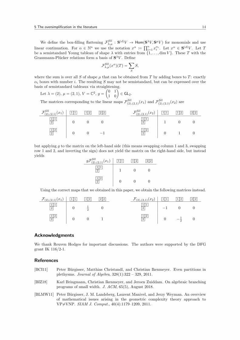
We define the box-filling flattening Ffillλ,µ : S(d)V → Hom(SλV,SµV ) for monomials and use

linear continuation. For α ∈ Nn we use the notation xα :=∏ni=1 x

αii . Let xα ∈ S(d)V . Let T

be a semistandard Young tableau of shape λ with entries from {1, . . . ,dimV }. These T with theGrassmann-Plucker relations form a basis of SλV . Define

Ffillλ,µ(xα)(T ) =

∑S

S,

where the sum is over all S of shape µ that can be obtained from T by adding boxes to T : exactlyαi boxes with number i. The resulting S may not be semistandard, but can be expressed over thebasis of semistandard tableaux via straightening.

Let λ = (2), µ = (2, 1), V = C2, g =

(0 11 0

)∈ GL2.

The matrices corresponding to the linear maps Ffill(2),(2,1)(x1) and Ffill

(2),(2,1)(x2) are

Ffill(2),(2,1)(x1) 1 1 1 2 2 2

1 12 0 0 0

1 22 0 0 −1

Ffill(2),(2,1)(x2) 1 1 1 2 2 2

1 12 1 0 0

1 22 0 1 0

but applying g to the matrix on the left-hand side (this means swapping column 1 and 3, swappingrow 1 and 2, and inverting the sign) does not yield the matrix on the right-hand side, but insteadyields

gFfill(2),(2,1)(x1) 1 1 1 2 2 2

1 12 1 0 0

1 22 0 0 0

Using the correct maps that we obtained in this paper, we obtain the following matrices instead.

F(2),(2,1)(x1) 1 1 1 2 2 2

1 12 0 1

2 0

1 22 0 0 1

F(2),(2,1)(x2) 1 1 1 2 2 2

1 12 −1 0 0

1 22 0 − 1

2 0

Acknowledgments

We thank Reuven Hodges for important discussions. The authors were supported by the DFGgrant IK 116/2-1.

References

[BCI11] Peter Burgisser, Matthias Christandl, and Christian Ikenmeyer. Even partitions inplethysms. Journal of Algebra, 328(1):322 – 329, 2011.

[BIZ18] Karl Bringmann, Christian Ikenmeyer, and Jeroen Zuiddam. On algebraic branchingprograms of small width. J. ACM, 65(5), August 2018.

[BLMW11] Peter Burgisser, J. M. Landsberg, Laurent Manivel, and Jerzy Weyman. An overviewof mathematical issues arising in the geometric complexity theory approach toVP6=VNP. SIAM J. Comput., 40(4):1179–1209, 2011.

5 The oversimplification in the literature 15

[EGOW18] Klim Efremenko, Ankit Garg, Rafael Oliveira, and Avi Wigderson. Barriers for RankMethods in Arithmetic Complexity. In Anna R. Karlin, editor, 9th Innovations inTheoretical Computer Science Conference (ITCS 2018), volume 94 of Leibniz Inter-national Proceedings in Informatics (LIPIcs), pages 1:1–1:19, Dagstuhl, Germany,2018. Schloss Dagstuhl–Leibniz-Zentrum fuer Informatik.

[ELSW18] Klim Efremenko, Joseph M. Landsberg, Hal Schenck, and Jerzy Weyman. The methodof shifted partial derivatives cannot separate the permanent from the determinant.Math. Comput., 87(312):2037–2045, 2018.

[Far16] Cameron Farnsworth. Koszul–Young flattenings and symmetric border rank of thedeterminant. Journal of Algebra, 447:664 – 676, 2016.

[GKKS14] Ankit Gupta, Pritish Kamath, Neeraj Kayal, and Ramprasad Saptharishi. Approach-ing the chasm at depth four. J. ACM, 61(6):33:1–33:16, 2014.

[GL19] Fulvio Gesmundo and Joseph M. Landsberg. Explicit polynomial sequences withmaximal spaces of partial derivatives and a question of K. Mulmuley. Theory ofComputing, 15(3):1–24, 2019.

[GMOW19] A. Garg, V. Makam, R. Oliveira, and A. Wigderson. More barriers for rank methods,via a ”numeric to symbolic” transfer. In 2019 IEEE 60th Annual Symposium onFoundations of Computer Science (FOCS), pages 824–844, 2019.

[Hod17] Reuven Hodges. A closed non-iterative formula for straightening fillings of Youngdiagrams. arXiv:1710.05214, 2017.

[Hod20] Reuven Hodges. A non-iterative formula for straightening fillings of Young diagrams.manuscript, based on arXiv:1710.05214, 2020.

[Lan12] Joseph M. Landsberg. Tensors : Geometry and Applications . Providence, R.I. :American Mathematical Society, 2012.

[Lan15] J. M. Landsberg. Geometric complexity theory: an introduction for geometers. Annalidell’ Universita di Ferrara, 61(1):65–117, May 2015.

[LMR13] J. M. Landsberg, Laurent Manivel, and Nicolas Ressayre. Hypersurfaces with degen-erate duals and the geometric complexity theory program. Commentarii MathematiciHelvetici, 88(2):469–484, 2013.

[LO13] J. M. Landsberg and Giorgio Ottaviani. Equations for secant varieties of veronese andother varieties. Annali di Matematica Pura ed Applicata, 192(4):569–606, Aug 2013.

[LO15] Joseph M. Landsberg and Giorgio Ottaviani. New lower bounds for the border rankof matrix multiplication. Theory of Computing, 11(11):285–298, 2015.

[MM14] Laurent Manivel and Mateusz Micha lek. Effective constructions in plethysms andweintraub’s conjecture. Algebras and Representation Theory, 17(2):433–443, Apr 2014.

[MS02] Ketan D. Mulmuley and Milind Sohoni. Geometric complexity theory I: An approachto the P vs. NP and related problems. SIAM J. Comput., 31(2):496–526, 2002.

[MS08] Ketan D. Mulmuley and Milind Sohoni. Geometric complexity theory II: Towardsexplicit obstructions for embeddings among class varieties. SIAM J. Comput.,38:1175–1206, July 2008.

[NW95] Noam Nisan and Avi Wigderson. Lower bounds on arithmetic circuits via partialderivatives. In Proceedings of the 36th Annual Symposium on Foundations of Com-puter Science, FOCS ’95, pages 16–25, Washington, DC, USA, 1995. IEEE ComputerSociety.

5 The oversimplification in the literature 16

[Oed16] Luke Oeding. Border ranks of monomials. arXiv:1608.02530v1, August 2016.

[Oed19] Luke Oeding. Border ranks of monomials. arXiv:1608.02530v3, January 2019.

[Olv82] Peter J. Olver. Differential Hyperforms I. Preprint. University of Minnesota, 1982.available at http://www-users.math.umn.edu/~olver/a_/hyper.pdf.

[Res20] Nicolas Ressayre. Vanishing symmetric kronecker coefficients. Beitrage zur Algebraund Geometrie / Contributions to Algebra and Geometry, 61(2):231–246, Jun 2020.

[Sam08] Steven V. Sam. PieriMaps: A Macaulay2 package. Version 1.0. A Macaulay2 pack-age available at https://github.com/Macaulay2/M2/tree/master/M2/Macaulay2/

packages, 2008.

[Str83] V. Strassen. Rank and optimal computation of generic tensors. Linear Algebra andits Applications, 52-53:645 – 685, 1983.

[Syl52] James J. Sylvester. On the Principles of the Calculus of Forms. Cambridge andDublin Mathematical Journal, 1852.

[Tow77] Jacob Towber. Two new functors from modules to algebras. Journal of Algebra,47:80–104, 1977.

[Tow79] Jacob Towber. Young symmetry, the flag manifold, and representations of gl(n).Journal of Algebra, 61(2):414 – 462, 1979.

[Wey03] Jerzy M. Weyman. Cohomology of Vector Bundles and Syzygies. Cambridge Tractsin Mathematics. Cambridge University Press, 2003.