THESE TERMS GOVERN YOUR USE OF THIS DOCUMENT Your use of this Ontario Geological Survey document (the “Content”) is governed by the terms set out on this page (“Terms of Use”). By downloading this Content, you (the “User”) have accepted, and have agreed to be bound by, the Terms of Use. Content: This Content is offered by the Province of Ontario’s Ministry of Northern Development and Mines (MNDM) as a public service, on an “as-is” basis. Recommendations and statements of opinion expressed in the Content are those of the author or authors and are not to be construed as statement of government policy. You are solely responsible for your use of the Content. You should not rely on the Content for legal advice nor as authoritative in your particular circumstances. Users should verify the accuracy and applicability of any Content before acting on it. MNDM does not guarantee, or make any warranty express or implied, that the Content is current, accurate, complete or reliable. MNDM is not responsible for any damage however caused, which results, directly or indirectly, from your use of the Content. MNDM assumes no legal liability or responsibility for the Content whatsoever. Links to Other Web Sites: This Content may contain links, to Web sites that are not operated by MNDM. Linked Web sites may not be available in French. MNDM neither endorses nor assumes any responsibility for the safety, accuracy or availability of linked Web sites or the information contained on them. The linked Web sites, their operation and content are the responsibility of the person or entity for which they were created or maintained (the “Owner”). Both your use of a linked Web site, and your right to use or reproduce information or materials from a linked Web site, are subject to the terms of use governing that particular Web site. Any comments or inquiries regarding a linked Web site must be directed to its Owner. Copyright: Canadian and international intellectual property laws protect the Content. Unless otherwise indicated, copyright is held by the Queen’s Printer for Ontario. It is recommended that reference to the Content be made in the following form: <Author’s last name>, <Initials> <year of publication>. <Content title>; Ontario Geological Survey, <Content publication series and number>, <total number of pages>p. Use and Reproduction of Content: The Content may be used and reproduced only in accordance with applicable intellectual property laws. Non-commercial use of unsubstantial excerpts of the Content is permitted provided that appropriate credit is given and Crown copyright is acknowledged. Any substantial reproduction of the Content or any commercial use of all or part of the Content is prohibited without the prior written permission of MNDM. Substantial reproduction includes the reproduction of any illustration or figure, such as, but not limited to graphs, charts and maps. Commercial use includes commercial distribution of the Content, the reproduction of multiple copies of the Content for any purpose whether or not commercial, use of the Content in commercial publications, and the creation of value-added products using the Content. Contact: FOR FURTHER INFORMATION ON PLEASE CONTACT: BY TELEPHONE: BY E-MAIL: The Reproduction of Content MNDM Publication Services Local: (705) 670-5691 Toll Free: 1-888-415-9845, ext. 5691 (inside Canada, United States) [email protected]The Purchase of MNDM Publications MNDM Publication Sales Local: (705) 670-5691 Toll Free: 1-888-415-9845, ext. 5691 (inside Canada, United States) [email protected]Crown Copyright Queen’s Printer Local: (416) 326-2678 Toll Free: 1-800-668-9938 (inside Canada, United States) [email protected]
Transcript
THESE TERMS GOVERN YOUR USE OF THIS DOCUMENT
Your use of this Ontario Geological Survey document (the “Content”) is governed by the terms set out on this page (“Terms of Use”). By downloading this Content, you (the
“User”) have accepted, and have agreed to be bound by, the Terms of Use.
Content: This Content is offered by the Province of Ontario’s Ministry of Northern Development and Mines (MNDM) as a public service, on an “as-is” basis. Recommendations and statements of opinion expressed in the Content are those of the author or authors and are not to be construed as statement of government policy. You are solely responsible for your use of the Content. You should not rely on the Content for legal advice nor as authoritative in your particular circumstances. Users should verify the accuracy and applicability of any Content before acting on it. MNDM does not guarantee, or make any warranty express or implied, that the Content is current, accurate, complete or reliable. MNDM is not responsible for any damage however caused, which results, directly or indirectly, from your use of the Content. MNDM assumes no legal liability or responsibility for the Content whatsoever. Links to Other Web Sites: This Content may contain links, to Web sites that are not operated by MNDM. Linked Web sites may not be available in French. MNDM neither endorses nor assumes any responsibility for the safety, accuracy or availability of linked Web sites or the information contained on them. The linked Web sites, their operation and content are the responsibility of the person or entity for which they were created or maintained (the “Owner”). Both your use of a linked Web site, and your right to use or reproduce information or materials from a linked Web site, are subject to the terms of use governing that particular Web site. Any comments or inquiries regarding a linked Web site must be directed to its Owner. Copyright: Canadian and international intellectual property laws protect the Content. Unless otherwise indicated, copyright is held by the Queen’s Printer for Ontario. It is recommended that reference to the Content be made in the following form: <Author’s last name>, <Initials> <year of publication>. <Content title>; Ontario Geological Survey, <Content publication series and number>, <total number of pages>p. Use and Reproduction of Content: The Content may be used and reproduced only in accordance with applicable intellectual property laws. Non-commercial use of unsubstantial excerpts of the Content is permitted provided that appropriate credit is given and Crown copyright is acknowledged. Any substantial reproduction of the Content or any commercial use of all or part of the Content is prohibited without the prior written permission of MNDM. Substantial reproduction includes the reproduction of any illustration or figure, such as, but not limited to graphs, charts and maps. Commercial use includes commercial distribution of the Content, the reproduction of multiple copies of the Content for any purpose whether or not commercial, use of the Content in commercial publications, and the creation of value-added products using the Content. Contact:
FOR FURTHER INFORMATION ON PLEASE CONTACT: BY TELEPHONE: BY E-MAIL:
LES CONDITIONS CI-DESSOUS RÉGISSENT L'UTILISATION DU PRÉSENT DOCUMENT.
Votre utilisation de ce document de la Commission géologique de l'Ontario (le « contenu ») est régie par les conditions décrites sur cette page (« conditions d'utilisation »). En
téléchargeant ce contenu, vous (l'« utilisateur ») signifiez que vous avez accepté d'être lié par les présentes conditions d'utilisation.
Contenu : Ce contenu est offert en l'état comme service public par le ministère du Développement du Nord et des Mines (MDNM) de la province de l'Ontario. Les recommandations et les opinions exprimées dans le contenu sont celles de l'auteur ou des auteurs et ne doivent pas être interprétées comme des énoncés officiels de politique gouvernementale. Vous êtes entièrement responsable de l'utilisation que vous en faites. Le contenu ne constitue pas une source fiable de conseils juridiques et ne peut en aucun cas faire autorité dans votre situation particulière. Les utilisateurs sont tenus de vérifier l'exactitude et l'applicabilité de tout contenu avant de l'utiliser. Le MDNM n'offre aucune garantie expresse ou implicite relativement à la mise à jour, à l'exactitude, à l'intégralité ou à la fiabilité du contenu. Le MDNM ne peut être tenu responsable de tout dommage, quelle qu'en soit la cause, résultant directement ou indirectement de l'utilisation du contenu. Le MDNM n'assume aucune responsabilité légale de quelque nature que ce soit en ce qui a trait au contenu. Liens vers d'autres sites Web : Ce contenu peut comporter des liens vers des sites Web qui ne sont pas exploités par le MDNM. Certains de ces sites pourraient ne pas être offerts en français. Le MDNM se dégage de toute responsabilité quant à la sûreté, à l'exactitude ou à la disponibilité des sites Web ainsi reliés ou à l'information qu'ils contiennent. La responsabilité des sites Web ainsi reliés, de leur exploitation et de leur contenu incombe à la personne ou à l'entité pour lesquelles ils ont été créés ou sont entretenus (le « propriétaire »). Votre utilisation de ces sites Web ainsi que votre droit d'utiliser ou de reproduire leur contenu sont assujettis aux conditions d'utilisation propres à chacun de ces sites. Tout commentaire ou toute question concernant l'un de ces sites doivent être adressés au propriétaire du site. Droits d'auteur : Le contenu est protégé par les lois canadiennes et internationales sur la propriété intellectuelle. Sauf indication contraire, les droits d'auteurs appartiennent à l'Imprimeur de la Reine pour l'Ontario. Nous recommandons de faire paraître ainsi toute référence au contenu : nom de famille de l'auteur, initiales, année de publication, titre du document, Commission géologique de l'Ontario, série et numéro de publication, nombre de pages. Utilisation et reproduction du contenu : Le contenu ne peut être utilisé et reproduit qu'en conformité avec les lois sur la propriété intellectuelle applicables. L'utilisation de courts extraits du contenu à des fins non commerciales est autorisé, à condition de faire une mention de source appropriée reconnaissant les droits d'auteurs de la Couronne. Toute reproduction importante du contenu ou toute utilisation, en tout ou en partie, du contenu à des fins commerciales est interdite sans l'autorisation écrite préalable du MDNM. Une reproduction jugée importante comprend la reproduction de toute illustration ou figure comme les graphiques, les diagrammes, les cartes, etc. L'utilisation commerciale comprend la distribution du contenu à des fins commerciales, la reproduction de copies multiples du contenu à des fins commerciales ou non, l'utilisation du contenu dans des publications commerciales et la création de produits à valeur ajoutée à l'aide du contenu. Renseignements :
POUR PLUS DE RENSEIGNEMENTS SUR VEUILLEZ VOUS
ADRESSER À : PAR TÉLÉPHONE : PAR COURRIEL :
la reproduction du contenu
Services de publication du MDNM
Local : (705) 670-5691 Numéro sans frais : 1 888 415-9845,
Queen's Printer for Ontario 1987 Printed in Ontario, Canada
MINES AND MINERALS DIVISION
ONTARIO GEOLOGICAL SURVEY
Open File Report 5674
Ontario Geoscience Research Grant Program Grant No. 260
Magnetotelluric Mapping of the Destor-Porcupine Fault
by
J.D. Redman, S.K. Zhao, and D.W. Strangway
1987
Parts of this publication may be quoted if credit isgiven. It is recommended that reference to this publicationbe made in the following form:
Redman, J.D., Zhao, S.K., and Strangway, D.W.
1987: Ontario Geoscience Research Grant Program, Grant No. 260 Magnetotelluric mapping of the Destor-Porcupine Fault; Ontario Geological Survey, Open File Report 5674, 37 pages and 14 figures.
Ontario Geological Survey
OPEN FILE REPORT
Open File Reports are made available to the public subject to the following conditions:
This report is unedited. Discrepancies may occur for which the Ontario Geological Survey does not assume liability. Recommendations and statements of opinions expressed are those of the author or authors and are not to be construed as statements of govern ment policy.
This Open File Report is available for viewing at the following locations:
(1) Mines LibraryMinistry of Northern Development and Mines 8th floor, 77 Grenville Street Toronto, Ontario MSS IBS
(2) The office of the Regional or Resident Geologist in whose district the area covered by this report is located.
Copies of this report may be obtained at the user's expense from a commercial printing house. For the address and instructions to order, contact the appropriate Regional or Resident Geologist's offices) or the Mines Library. Microfiche copies (42x reduction) of this report are available for $2.00 each plus provincial sales tax at the Mines Library or the Public Information Centre, Ministry of Natural Resources, W-l 6 40, 99 Wellesley Street West, Toronto.
Handwritten notes and sketches may be made from this report. Check with the Mines Library or Regional/Resident Geologist's office whether there is a copy of this report that may be borrowed. A copy of this report is available for Inter-Library Loan.
This report is available for viewing at the following Regional or Resident Geologists* offices:
All Regional/Resident Geologists 1 Offices.
The right to reproduce this report is reserved by the Ontario Ministry of Northern Development and Mines. Permission for other reproductions must be obtained in writing from the Director, Ontario Geological Survey.
V.G. Milne, Director Ontario Geological Survey
fci
ONTARIO GEOSCIENCE RESEARCH GRANT FUND
Final Research Report
Foreword
This publication is a final report of a research project that was funded under the Ontario Geoscience Research Grant Program. A requirement of the Program is that recipients are to submit final reports within six months after termination of funding.
A final report is designed as a comprehensive summary stating the findings obtained during the tenure of the grant, together with supporting data. It may consist, in part, of reprints or preprints of publications and copies of addresses given at scientific meetings.
It is not the intent of the Ontario Geological Survey to formally publish the final reports for wide distribution, but rather to encourage the recipients of grants to seek publication in appropriate scientific journals whenever possible. The Survey, however, also has an obligation to ensure that the results of the research are made available to the public at an early date. Although final reports are the property of the applicants and the sponsoring agencies, they may also be placed on open file. This report is intended to meet this obligation.
No attempt has been made to edit the report, the content of which is entirely the responsibility .f the author(s).
A. Tensor AMT Technique ....................................... 25
B. Abstract of Presented Paper ................................. 37
-vii-
FIGURE CAPTIONS:
1. Location map for AMT lines and tensor station. The faults shown are taken from Map 2205 (Pyke et al, 1973)...........xv
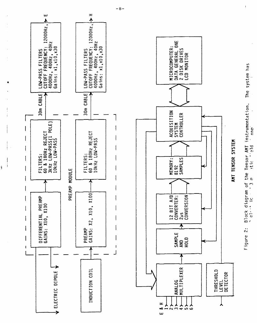
2. Block diagram of the Tensor AMT instrumentation. The system has three electric and three magnetic field channels..........8
3. Flow chart describing the in field data processing that takes place as the time series data are being collected.........9
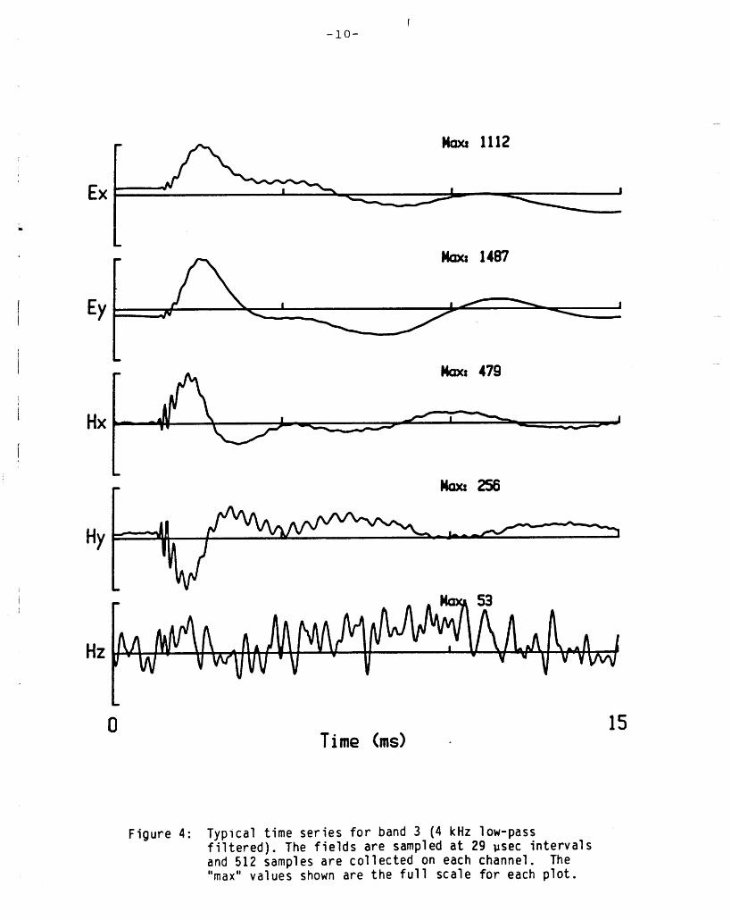
4. Typical time series for band 3 (4kHz low-pass filtered). The fields are sampled at 29 u^sec intervals and 512 samples are collected on each channel. The "max" values shown are the full scale for each plot........ . . . . . . . . . . . . . . . . . . . . . . . . . . . . . . .10
5a. AMT profiling results for line 1. The -computed resistivities for the two dimensional model and the field data for the two measurement orientations are shown........... . . . . . . . . . . . . . 12
5b. Two-dimensional resisitivity model (vertical cross section in the north-south direction) used to fit field data for line 1. The numbers shown in each region are resistivities in ohm-m. The model has infinite extent in the east-west direction...13
6. AMT profiling results for line 2. Field data for the twomeasurement orientations are shown. ... ... ... . . . . . . . . . . . . . . . 16
7. The anisotropy observed in the apparent resistivities forlines l and 2....................... ........................17
8a. Tensor AMT results for station 1. The strike of the minoraxis is only given for frequencies at which the resistivity structure is clearly two-dimensional. Only data for which the coherency was greater than .95 have been plotted......20
8b. Tensor/^MT results for station 2. The strike of the minoraxis is only given for frequencies at which the resistivity structure is clearly two-dimensional. Only data for which the coherency was greater than .95 have been plotted.......21
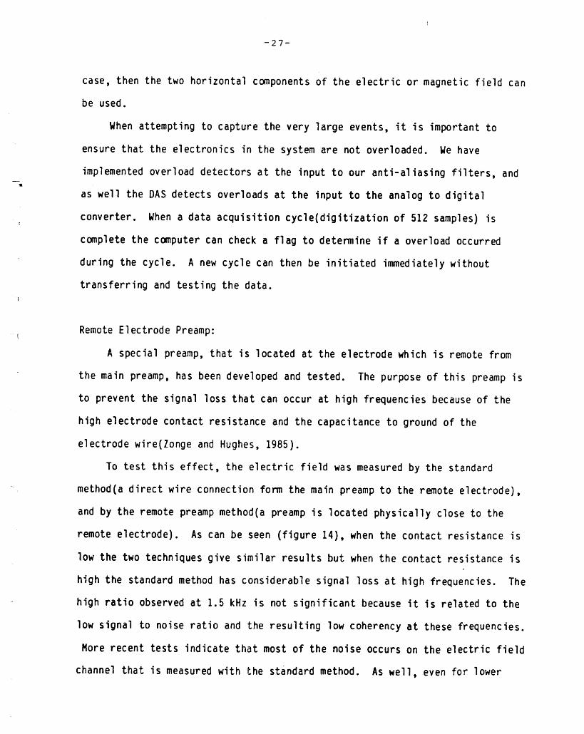
9. Typical time series (512 samples) recorded in band 4 at the output of the low-pass filters. The vertical electric field is also measured for use as trigger source and potentially as a reference...................... ......................29
10. Magnetic field amplitude spectra for 10 separate eventsrecorded in band 4. The characteristic 2 kHz null is clearly seen.............................. .......................30
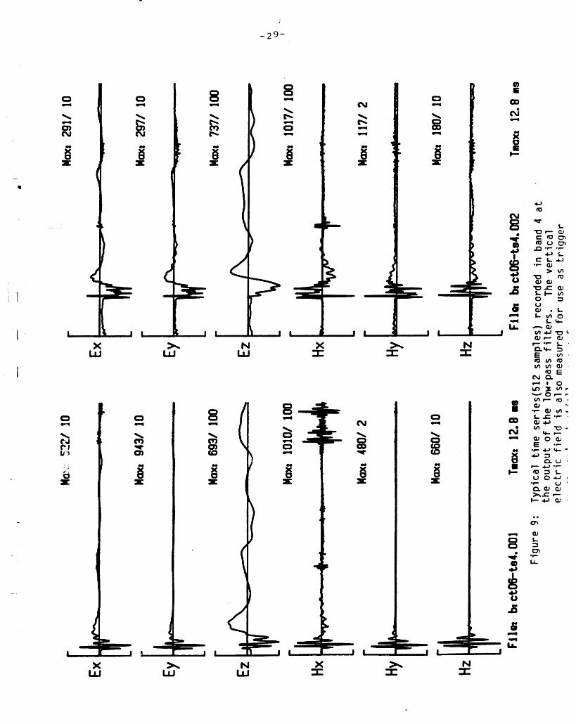
11. Magnetic field amplitude spectra (each spectrum is an average for approximately 20 events) on 4 days. Both the shape and the level of the spectra have a large variation. . . . . ... . . . . . .. .31
-ix-
12. Magnetic field time series (4096 samples) showing the large events in a relatively quite background. It is these large events that the data acquistion system is designed to capture..32
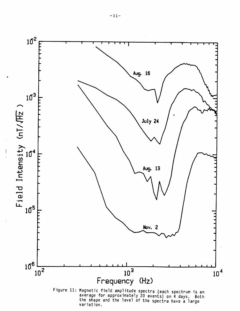
13a. Comparison of the magnetic field amplitude spectra in band2 obtained by acceptance of all data (normal) and by selection of only the large magnitude events (triggered) . ... ... . . . .. . . . . 33
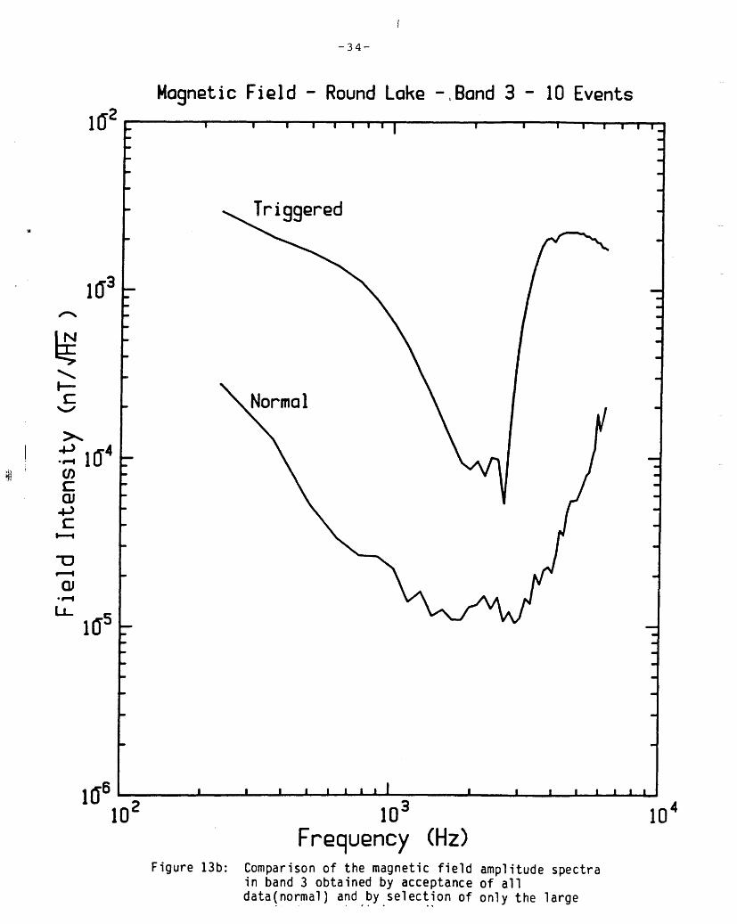
13b. Comparison of the magnetic field amplitude spectra in band3 obtained by acceptance of all data (normal) and by selection of only the large magnitude events (triggered) ... . .. . .. . . . 34
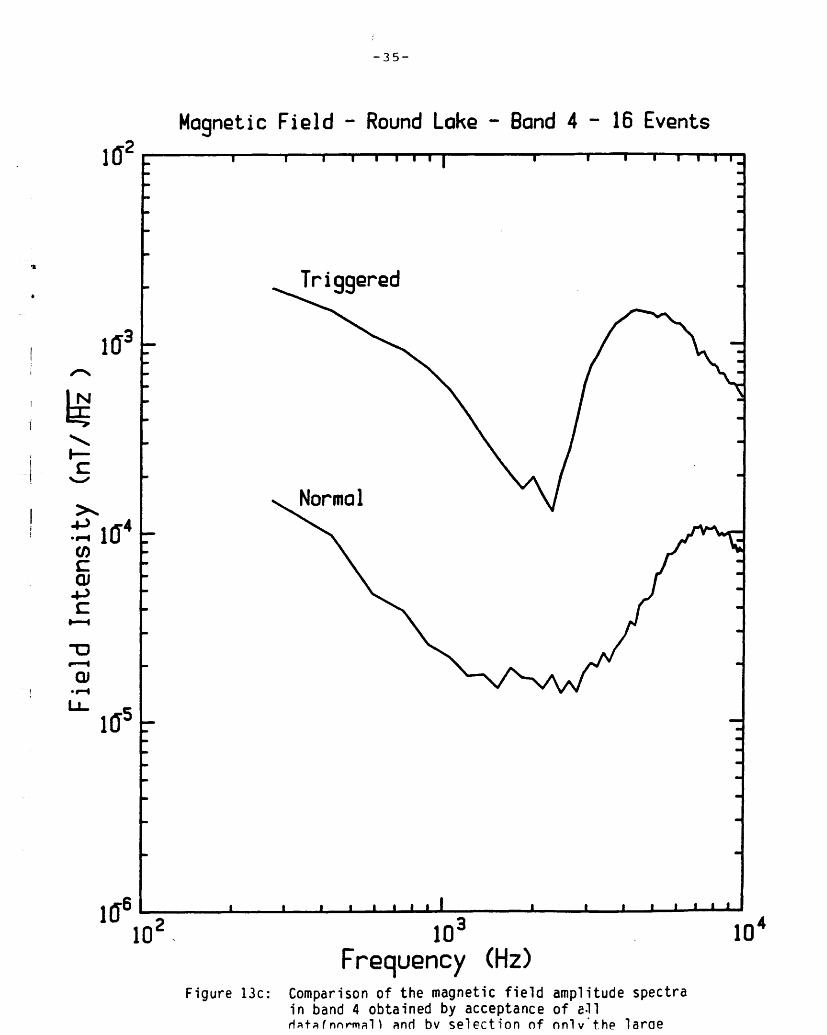
13c. Comparison of the magnetic field amplitude spectra in band4 obtained by acceptance of all data (normal) and by selection of only the large magnitude events (triggered) . .. .. . . . . . . . . .35
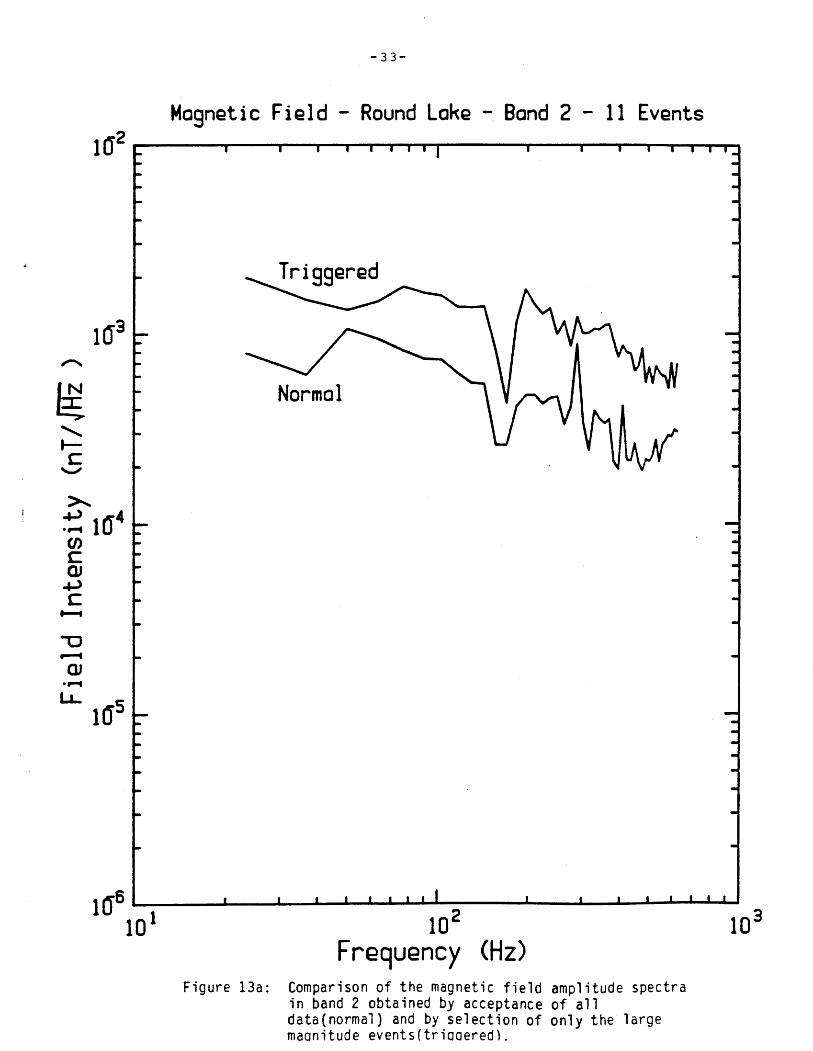
14. Comparison of electric field measurements (band 4) with aremote electrode preamp and the normal method (29m wire length).Clearly, in areas where the contact resistance is high, thenormal method in which a direct unshielded wire connectionis made to the remote electrode has significant loss ofsignal at the high frequencies................................36
-xi-
Abstract
An audio-frequency magnetotelluric(AMT) survey was carried out in Stock Township on two lines that cross the Destor-Porcupine fault(DPF). In the area studied the fault is covered by 20-50 m of conductive overburden. The purpose of the survey was to determine the location and structural features of any conductive zone associated with the DPF. There were 64 stations located on the two lines which were each approximately 2 km in length. Apparent resistivities were measured for two orthogonal directions of the electric field dipoles at 83 Hz and 8.6 kHz. The interpretation of these profiles shows that on one of the lines there is a relatively wide, conductive and anisotropic zone in -the basement. This zone is centered on the previously mapped(Pyke et al, 1973) location of the DPF. On the other line we did not find a distinctive conductive zone that could be attributed to the fault zone. Tensor AMT measurements at two stations show that the strike of the most conductive axis is east-west at low frequencies indicating the principal direction of fractures or an intrinsic anisotropy in the metasediments. The Destor-Porcupine fault appears to be a good electrical conductor on one line and on this line AMT can detect its presence below a significant thickness of overburden. The effect of the fault on the apparent resistivity profiles, when there is a significant thickness of conductive overburden, is subtle and requires very careful measurements with the Scalar AMT method. If the AMT technique is to be applied routinely in these kinds of environments, then it will be necessary to use the normal Tensor AMT method or a profiling method that is a derivative of this technique and thus can provide the higher accuracy that is required.
-xiii-
1-METAVOLCANICS2-METASEDIMENTS
O 1km
Figure 1: Location map for AMT lines and tensor stations. The faults shown are taken from Map 2205(Pyke et al, 1973).
-xv-
MAGNETOTELLURIC MAPPING OF THE DEBTOR-PORCUPINE FAULT
READ DAS STATUS WITH COMPUTER. DID OVERLOAD OCCUR IN DAS OR IN ANALOG FILTERS?
YES
NO
MOVE TIME SERIES FROM DAS TO COMPUTER.
DISPLAY TIME SERIES. IS TIME SERIES ACCEPTABLE?
NO
YES
COMPUTE DFT FOR 6 CHANNELS
COMPUTE AVERAGED AUTO AND CROSS POWERS WITHIN EACH SUB-BAND.
SAVE AUTO AND CROSS POWERS ON DISK AND ADD TO ACCUMULATORS.
DISPLAY POWER SPECTRA AND TENSOR APPARENT RESISTIVITIES.
COLLECT MORE DATA?YES
NO
TENSOR AMT DATA COLLECTION PROCEDURE
Figure 3: Flow chart describing the in field data processing that takes place as the time series data are being collected.
-10-
Hoxt 1112
OTime Cms)
15
Figure 4: Typical time series for band 3 (4 kHz low-passfiltered). The fields are sampled at 29 ysec intervals and 512 samples are collected on each channel. The "max" values shown are the full scale for each plot.
-11-
3. RESULTS AND INTERPRETATION
3.1 Scalar AMT Profiling:
Two profiles near Shillington (Figure 1) were measured over the fault zone
that is indicated on geology maps. The geology maps indicate that the fault
structures around line 2 are more complex than around line l and that there is
a change in the character of the fault zone where line l crosses the fault.
Since this region encompassing line l and 2 is buried under 20-50 m of
overburden, there is no direct evidence to locate the fault and the strength of
the evidence for mapping the faults in the location shown on geology maps is
uncertain. In fact, the location and configuration of the faults in this
region are probably not known with accuracy.
The profiles for line l and 2 are shown in figures 5a and 6. In general,
at 83 Hz the apparent resistivities reflect the variation in the bedrock
resistivity and at 8570 Hz they are mainly influenced by variations in the
overburden resistivity or thickness. On both of these lines conductive zones
in the bedrock are indicated by the anisotropy (differences in resistivity for
the two measurement directions) shown in figure 7. The apparent resistivities
at 83 Hz, in the east-west direction are in general lower indicating that there
are conductive structures with relatively long strike length in this direction.
For line l, the presence of a conductive zone is quite evident by simply
examining the 83 Hz profile. The high frequency profile is quite uniform
indicating that the overburden resistivity is relatively constant and that the
overburden thickness does not decrease to any great extent along the line.
The differences in the profiles for the two measurement directions are
characteristic of two-dimensional structures. The computed response for the
-12-
Line l * Field Data Model10
E
E
C/)
SO 910 2
01
oQ. d.
. *
-400
10
E lE
O
O) O!
10-P
Ql
OQ.d.
-400 S
Electric Dipole EW
83 Hz
* *-
8570 Hz
I400 800 Distance (m)
1200 1600
Electric Dipole NS
83 Hz
8570 Hz
I i 1400 800 Distance (m)
1200 1600N
Figure 5a: AMT profiling results for line 1. The computedresistivities for the two-dimensional model and the field data for the two measurement orientations are
-13-
two-dimensional mode1(Figure 5b) of the resistivity structure for line l,
shown in figure 5a, fits our field data quite well for both measurement
orientations. The model response was computed using the finite element
technique(Zhao, 1983 and Xu, 1985). A trial and error technique was used to
arrive at the optimum model shown.
.C •PO.Oa
200
400•400
S
NS-4000EW-1000
i
NS-2200 EW-170
400 600 Distance (m)
8000
1200 1600N
Figure 5b: Two-dimensional resistivity model (vertical cross section in the north-south direction) used to fit field data for line 1. The numbers shown in each region are resistivities in ohm-m. The model has infinite extent in the east-west direction.
In the modelling process an attempt was made to keep the model as simple
as possible while still providing a reasonable fit with the data. There is
likely some topography on the bedrock surface but the uniformity of the 8 kHz
data implies that the thickness of the overburden is relatively uniform.
The main conductive feature in the bedrock observed on line l between 675N
and 1175N has been modelled by a zone in which the resistivity is anisotropic.
The east-west resistivity is 170 ohm-m compared to 2200 ohm-m in the north-
south direction. This observed anisotropy is probably a macroscopic anisotropy
caused by the principal direction of fracturing. This zone of apparent
anisotropic resistivity in the basement could also be modelled with a region of
-14-
vertical dike-like conductive structures embedded in a resistive background
medium. A zone of vertical fractures striking east-west would be an example of
this kind of structure. We were also able to fit our apparent resistivity
profiles with this kind of model. But, in practice, information about the
specific fractures in this zone can not be obtained since there are many models
of this kind that would fit our data. Thus this zone is treated, simply as a
zone in which the resistivity is anisotropic. The 45" dip to the south of this
conductive zone produces an asymmetry in the profile that provides a better fit
to our data than could be obtained with a vertical structure. The zone south
of the major conductive zone is also anisotropic reflecting possibly less
extensive fracturing in the east-west direction.
The profiles for line 2 are more complicated than line l, and as seen on
the anisotropy plots for the 83 Hz data the east-west direction is also more
conductive. The 8570 Hz profile is more variable showing that the overburden
conductivity or thickness is less uniform. There are conductive zones centered
at 1600S and 700S on this line. We have attempted to fit a two-dimensional
model to this data as well, but we were unable to get a good fit to the
apparent resistivity profile. This profile is much more complicated than for
line l and does not show the same distinctive conductive zone. The overburden
thickness and/or resistivity are more variable on this line and this effect
obscures the response of the basement structure.
On line l the DPF appears to be an anisotropic conductive zone, 500 m
wide, centered about 900N. This is consistent with a wide fracture zone with
fractures that strike in the east-west direction. The geology map for this
area places the DPF at approximately 900N. The DPF has been observed in the
subsurface, 5 km to the west at the St Andrew Goldfields deposit, as a system
of chlorite and talc-chlorite shear zones with a width of approximately 150 m
-15-
(Malczak, 1985). This is consistent with the kind of structure suggested by
our interpretation. A similar conductive zone was not observed on line 2. If
the main conductive zone on line l is the DPF, then the profile for line 2
indicates that the DPF is clearly not as conductive on line 2. In fact, there
is no feature seen in the profile that we can clearly attribute to the DPF.
-16-
Ling 2 * FiQld Data10
i
o
O)•f*
O)01 210 2
01
O O-a.
10 l
Electric Dipole EW
83 Hz
: ****S***S^8570 Hz
l l l-2200 -1800 -1400 -1000
Distance (m)-600 -200
10
-P O) * i(O 01
10
OQ.Q.
10l
ElGctric DipolG NS
83 Hz
8570 Hz -
l l i-2200
S-1800 -1400 -1000
Distance (m)-600 -200
N
Figure 6: AMT profiling results for line 2. Field data for the two measurement orientations are shown.
-17-
10CO
LU
OL.-PO(f)
id
Line 2 - Shillington - 1985
i-2200 -1800
83 Hz
-1400 -1000Distance (m)
* 8570 Hz
-600 -200
10CO : Line l - Shillington - 1985
-400 S
0 400 800 1200 Distance (m)
1600N
Figure 7: The anisotropy observed in the apparent resistivities for lines l and 2.
-18-
3.2 Tensor AMT:
Tensor AMT data were collected at two stations. Station l is at the north
end of line l and is situated well within the metasedimentary zone. Station 2
is at 600S on line 2. The station locations were limited to areas in which we
could obtain access with a vehicle since our equipment is mounted in a truck.
The results of these measurements are summarized in figures 8a and 8b.
The impedance tensor has been rotated into its principal directions to give the
major and minor apparent resistivity curves and the strike of the more
conductive direction or minor axis. The strike is only plotted for frequencies
at which the resistivity structure is clearly two-dimensional. A high skew
indicates that the structure is three dimensional. The skews observed for
these stations indicate that the structure is one or two-dimensional.
Both stations show that at high frequencies( above 200 Hz), the structure
is effectively one dimensional. That is, the overburden is a simple layered
structure. At the lower frequencies, there is increasing anisotropy indicating
that the structure is two-dimensional. For both stations the most conductive
direction, at low frequencies, is east-west. For station 2 this is probably
reflecting a conductive zone that is also indicated on the profiles. For
station l, the effect may be the result of an intrinsic anisotropy(possibly on
a large physical scale) similar to what we have observed for metasediments in
Moody township ( Strangway, 1983).
A one-dimensional or layered earth model has been fitted to the average of
the logarithm of the apparent resistivity of the major and minor axes. For
both stations, a simple two layer model, of conductive overburden over
resistive basement, was used to fit the dependence of apparent resistivity on
frequency. For station l , the upper layer is 29 m thick with a resistivity of
41 ohm-m and the lower layer has a resistivity of 7000 ohm-m. For station 2,
l-19-
the upper layer is 31 m thick with a resistivity of 50 ohm-m overlying a
8500 ohm-m section. This one dimensional fitting is used as input for the two-
dimensional modelling process.
-20-
IE
O
10
-PCdil-
i i iiiiiii i i i i i 11 ii i i i i 111 ii
Stn. l - Shillington - 1985i i iiiiiii __i i iiiiiii__i i i i 11 in i i i i 1111
01180
•^ 90-P10
10 10 10 10Frequency (Hz)
Strike of Hinor Axis
10
ut i i i i i.i iii i i i i 1 1 iii i i i i 1 1 iii i 1 1 iii
i i iiiiiii ___ i i i i 1 1 til iiiiiii
10 i10' 10 10 Frequency (Hz)
10
.5
oi
.0
1^ l l l l l III l l l l l f TIITTI l l l l l fill l l l II l 111 l l l l l l IIl II l 111
l l l l l l l M_____l l l l l l l M -l l 111 l l l l t\ 11
10 10 10 10 Frequency (Hz)
10
Figure 8a: Tensor AMT results for station 1. The strike of the minor axis is only given for frequencies at which the resistivity structure is clearly two-dimensional. Only data for which the coherency was greater than .95 have been plotted.
-21-
l
En o
10
C/) •*Hw
-pC 01
l l l l l l II l l III IT*
Hojor
Minor
! Stn.2 -Shillington - 1985i i i i 11 in i.ii i 11 ...l
10' 10 10 10Frgquency (Hz)
180QJ *T'Z 90 -P
Strike of Minor Axisl l l l l l l l l 111
111 l Illll i l l l l l III___l l l l l l III
10 10 10 10Frequency (Hz)
i i 11111
10
l l l l l l M l l l l l l l l
i l lil
10
.0
i i ri l l III T I f l I III! l l l l l 11 IT I l l l l l 11
i i i 11 til
10 10 10 10Frequency (Hz)
10
Figure 8b: Tensor AMT results for station 2. The strike of the minor axis is only given for frequencies at which the resistivity structure is clearly two-dimensional. Only data for which the coherency was greater than .95 have been plotted.
-22-
4. CONCLUSIONS
The interpretation of the apparent resistivity profile for line l clearly
indicates the presence of a wide conductive and anisotropic zone centered at
900N that is attributed to the Destor-Porcupine fault zone. This kind of
structure is also consistent with direct observations of the fault zone in this
area. A conductive zone associated with the presumed location of the DPF on
line 2 was not seen on our profile. Although the interpretation for line 2 is
more difficult, there is clearly not a significant conductive zone in the
basement similar to that seen on line 1. The DPF must be much less conductive
than on line 1. The tensor data for station l show that the strike of the most
conductive axis is east-west at low frequencies indicating the principal
direction of fractures or an intrinsic anisotropy in the metasediments.
This survey has shown that the DPF is a good electrical conductor in one
region and that in this region AMT can detect its presence below a significant
thickness of overburden. f
A fault that is buried below a significant thickness of conductive
overburden, as is the case in this area, produces a subtle effect on the
apparent resistivity profile. The AMT technique, in principal, is an excellent
tool for probing structure such as this. But, if AMT is to be applied
routinely to these kinds of problems then it will require a system that can
provide more accuracy than is available with the present Scalar AMT instruments.
The Tensor AMT technique can provide this accuracy but this method is expensive
to apply routinely to these kinds of structural problems. A fast profiling
method, that is a derivative of the Tensor AMT method and thus also provides
the same kind of accuracy, would be very useful for addressing these problems.
-23-
5. References:
Baker, C.L., Steele, K.G., Mcclenaghan, M.B. and Fortescue, J.A.C., 1985, Location of gold grains in Sonic Drill Core Samples form the Matheson area, Cochrane District, Ontario Geological Survey, Map P2736.
Fyon, J.A. and J.H. Crocket, 1983, Gold exploration in the Timmins area: Using field and lithological characteristics of carbonate alteration zones, Ontario Geological Survey-Study 26.
Kurtz, R.D., and E.R. Niblett, 1984, A Magnetotelluric survey over the East Bull Lake Gabbro-Anorthosite Complex, TR-236, Scientific Document Distribution Office, Atomic Energy of Canada Limited, Research Company, Chalk River, Ontario.
Labson, V.F., A. Becker, H.F. Morrison, and U. Conti, 1985, Geophysical exploration with audio-frequency natural magnetic fields, Geophysics, Vol.50, p.656-664.
Malczak, J., 1985, Preliminary Report on the St. Andrew Goldfields and Maude Lake Gold Deposits, District of Cochrane; in Summary of Fieldwork and Activities 1985, Ontario Geological Survey, edited by John Wood, Owen L. White, R.B. Barlow and A.C. Colvine, Ontario Geological Survey, Miscellaneous Paper 126, p316-319.
Middleton, R.S., 1976, Gravity survey of geological structures in the Timmins and Matheson Area, District of Cochrane, Timiskaming and Sudbury, Ontario Geological Survey, GR135.
Pyke, D.R., 1982, Geology of the Timmins Area, District of Cochrane, Ontario Geological Survey, Report 219.
Pyke, D.R., L.D. Ayres, and D.G. Innes, 1973, Timmins-Kirkland Lake Sheet, Cochrane, Sudbury, and Timiskaming District; Ontario Geological Survey, Geological Compilation Series, Map 2205.
Redman, J.D., D. Hsu, and D.W. Strangway, 1980, Audio frequency magnetotelluric measurements on the Eye-Dashwa Lakes pluton Atikokan, Ontario, Unpublished report , Geology Dept., Univ. of Toronto.
Strangway, D.W., C.M. Swift and R.C. Holmer, 1973, The application of audio-frequency magnetotellurics (AMT) to mineral exploration, Geophysics, Vol.37, p.98-141.
Strangway, D.W., O.M. Ilkisik, and Redman, J.D., 1983, Surface electromagnetic mapping in selected positions of Northern Ontario, 1982-1983, Ontario Geological Survey, Miscellaneous Paper 113.
Sutherland D.B., 1967,AFMAG for electromagnetic mapping, Mining and Groundwater Geophysics/1967, Geological Survey of Canada,.Economic Geology Report No. 26, p.228-237.
-24-
Vozoff, K., 1972, The Magnetotelluric method in the exploration of sedimentary basins, Geophysics, Vol.37, p.98-141.
Xu Shizhe, and Zhao Shengkai, 1985, Solution of magnetotelluric field equations for a two-dimensional, anisotropic geoelectric section by the finite element method, Acta Seismologica Sinica, Vol.7, p.80-90.
Zhao Shengkai, and Xu Shizhe, 1983, Two-dimensional magnetotelluric modelling by finite element method, Computing Techniques for Geophysical and Geochemical Exploration, No.l, p.14-21.
Zonge, K.L., and Hughes, J.L., 1985, Effect of electrode contact resistance on electric field measurements, Expanded Abstract, 55th Annual SEG Meeting.
-25-
6. APPENDICES
6.1 APPENDIX A - TENSOR AMT TECHNIQUE:
Introduction:
Application of the Tensor AMT technique to the problem of mapping the DPF,
also involved further development of the Tensor AMT technique. There has
already been considerable work carried out on this technique in the band from
l Hz to 500 Hz, but little has been published on the technique for the higher
frequencies up to 10 kHz. The particular difficulties in obtaining good
quality data in this higher band and the methods for improving data quality
will be discussed.
Characteristics of Natural Fields in the High Band (300 Hz-10 kHz):
Typical large events (figure 9) that were obtained in band 4 have energy
concentrated at both low and high frequencies with a low energy band in
between. The well known 2 kHz null is clearly seen in the magnetic field
amplitude spectra(figure 10) for individual events. The width and depth of
this null is quite variable for different events, as one would expect, since
the spectral shape depends both on the source characteristics and the
propagation path.
The events shown in figure 10 were collected over a period of approximately
one hour. The long term variability in the field intensities is much greater
as indicated in figure 11(average spectra for approximately 20 events). This
is one of the characteristics of the AMT source fields that makes the
measurements difficult. Even during the summer months there is a considerable
variation in signal strength. Because of the low field intensity for
-26-
frequencies between l kHz and 4 kHz, it is often difficult to obtain useful
apparent resistivity data at these frequencies.
Capturing Large Events:
Our equipment was designed to capture large magnitude events in real time.
Because the DAS(Data Acquisition System) operates independently from the field
computer, it continues to recycle until an event occurs that has sufficient
amplitude. After initiating the acquisition cycle(512 samples on 6 channels),
the DAS will start a new acquisition cycle at sample 128, if the threshold was
exceeded on the threshold channel during the first 64 samples or if it was not
exceeded between sample 65 and sample 128. Since the DAS and computer operate
in parallel, then the data that has been accepted can be analyzed while new
data is being acquired. In practice, this can speed up the operation
significantly since the large amplitude events occur infrequently.
Figure 12 shows that the large events in band 4 are well spaced in time.
When measurements are made at lower frequencies or when signal strengths are
low, it is sometimes necessary to wait for up to 5 minutes for a sufficiently
large event. As shown in figure 13a,b,c, it is possible to increase the signal
level dramatically, particularly at high frequencies, by only accepting the
large magnitude events for processing. Clearly, this also increases the signal
to noise ratio for instrumental and wind induced noise, and for cultural
noise(60 Hz and its harmonics).
To implement this technique on our system, it is necessary to select one
channel for the threshold detection. Recently, we have been using the vertical
electric field for this purpose, since it does not bias the accepted events in
favour of any particular source direction. However, the vertical electric
field can be considerably influenced by wind induced noise. If this is the
-27-
case, then the two horizontal components of the electric or magnetic field can
be used.
When attempting to capture the very large events, it is important to
ensure that the electronics in the system are not overloaded. We have
implemented overload detectors at the input to our anti-aliasing filters, and
as well the DAS detects overloads at the input to the analog to digital
converter. When a data acquisition cycle(digitization of 512 samples) is
complete the computer can check a flag to determine if a overload occurred
during the cycle. A new cycle can then be initiated immediately without
transferring and testing the data.
Remote Electrode Preamp:
A special preamp, that is located at the electrode which is remote from
the main preamp, has been developed and tested. The purpose of this preamp is
to prevent the signal loss that can occur at high frequencies because of the
high electrode contact resistance and the capacitance to ground of the
electrode wire(Zonge and Hughes, 1985).
To test this effect, the electric field was measured by the standard
method(a direct wire connection form the main preamp to the remote electrode),
and by the remote preamp method(a preamp is located physically close to the
remote electrode). As can be seen (figure 14), when the contact resistance is
low the two techniques give similar results but when the contact resistance is
high the standard method has considerable signal loss at high frequencies. The
high ratio observed at 1.5 kHz is not significant because it is related to the
low signal to noise ratio and the resulting low coherency at these frequencies.
More recent tests indicate that most of the noise occurs on the electric field
channel that is measured with the standard method. As well, even for lower
-28-
contact resistances of 10 kohm, the electric field would be reduced by 152 at
10 kHz if the direct wire connection was used.
-29-
co
CD
CNJ
N
.5 5
(O
73 r— O)C IO C^re o o*
C t. -4J•t- Q;
^D ^3
O) O)•o -c o) J- H- too 3 uO) . J-i- to o i- M-
•~* O)
QJ ^~ QJr- **~ l.O.**- 3E to(O tO (Cto to d)
10 E CSJ Q.•-H l OLO 5 t/* "•-^ O f— 'to i— co•^ tt) t/) "
O 4J
O) O O)
-M 3^^ CJ
03 3 ^O O *-*
•r- OCL O) O)
h- 4J O.'
O^
(UL. 13
N
-30-
Iff'
COcQ) •PC
"D
Q)
ti
10'
i i i i i i i i i i i i r
i i t i t i i
10 10FrQquency (Hz)
Figure 10: Magnetic field amplitude spectra for 10 separateevents recorded in band 4. The characteristic 2 kHz null is clearly seen.
-31-
Iff1
ICP
C/)Cdi -pc
iff'
iff'10
j i i i i i l
10 10FroquQncy (Hz)
Figure 11: Magnetic field amplitude spectra (each spectrum is an average for approximately 20 events) on 4 days. Both the shape and the level of the spectra have a large variation.
-32-
Or\j
c/)
JBUUDIJ3
Figure 12: Magnetic field time series(4096 samples) showing the large events in a relatively quite background. It is these large events that the data acquisition system is designed to capture.
-33-
l Cl
:tTlff4(OcOJ-pc
ID
QJ
iff:
iff'
MognQtic FiQ!d - Round Lake - Band 2-11 Events
10
Triggered
Normal
10 10FrQquQncy (Hz)
Figure 13a: Comparison of the magnetic field amplitude spectra in band 2 obtained by acceptance of all data(normal) and by selection of only the large maanitude eventsftriaaered).
-34-
MognQtic FiQ!d - Round Lakg -.Band 3-10 EvgntsIff2 r
lff;
C/)cQ)
TD Ql
iff:
iff'10
i i i i i i
Trigggrgd
• l10
FrgquGncy (Hz)
t l L
10
Figure 13b; Comparison of the magnetic field amplitude spectra in band 3 obtained by acceptance of all data(normal) and by selection of only the large
-35-
l(Tr
lff;
N
•tTlff4COC 01
4-)cl—l
TDr—l
QJ
Iff5
Iff'10
Magnetic Field - Round Lake - Band 4-16 Events
Triggered
i iii
10 10FrgquQncy (Hz)
Figure 13c: Comparison of the magnetic field amplitude spectra in band 4 obtained by acceptance of e-11
normal) and bv selection of onlv't.he larae
-36-
LU
CMUJ
LU
O• t—l4-)oo:•oQ)
•i—ili-
O• H
C-p oOJ
LU
E - RemotQ Electrode Preomp
10' 10' 10'
ocO)t-QJ
.CO
CJ
1.0
.9
Q
^x -7—: \r :-
i i iiiiiii i i iiiiii1.5
10' 1010'
1.0
El - Standard MethodE2 - Remote Electrode Preamp
Contact Resistance—110 kohm-— 10 kohm
10' ID-
FrQquGncy (Hz)
Figure 14: Comparison of electric field measurements(band 4) with a remote electrode preamp and the normal method(29m wire length). Clearly, in areas where the contact resistance is high, the normal method in which a direct unshielded wire connection is made to the remote electrode has significant loss of signal at the high frequencies.
-37-
6.2 APPENDIX B:
Paper presented at the Eighth Workshop on Electromagnetic Induction in the Earth and Moon, Neuchatel, Switzerland, August 1986.
Natural Fields in the Audio Band - Characteristics and Relevance to Tensor AMT Instrumentation DesT^n
J. D. RedmanDepartment of Geology, University of Toronto,Toronto, Ontario, CanadaD. W. StrangwayOffice of the President, University of BritishColumbia, Vancouver, British Columbia, Canada
A tensor magnetotelluric instrument that measures in the AMT band has been developed at the University of Toronto. This equipment has been used to study the characteristics of natural EM fields that are relevant to the design of tensor AMT instruments. The six channel instrument measures from l Hz to 10 kHz in four separate bands. In the audio frequency band, the principal source of natural EM energy at the earths surface is from worldwide thunderstorm activity. The observed magnetic and electric field events, which are usually related to individual lightning strikes, have an extremely large range of signal amplitudes during a normal measurement period. Typical field spectra for these events will be shown. The particular characteristics observed for the low signal strength band centered around 2 kHz will also be discussed. Real time analysis of all the received data on six channels in our highest band would require the processing of 468 time series (of length 512) per second which is clearly not feasible with field microcomputers. A large number of these time series would, in any case, have an insufficient signal to noise ratio to be useful. Since the data rate in the audio band is high, one can afford to wait for the events with the largest amplitudes. AMT tensor systems have thus required some means of selecting good data segments in real time. In our system, this procedure is carried out in hardware so that "good" signals are not ignored except when the data buffer is full. Using this technique and exercising sufficient patience, we were able to collect useful tensor data in Northern Ontario during November, when signal strengths are quite low. Typical power spectra, with and without data segment selection will be presented to illustrate this point.