Noname manuscript No.(will be inserted by the editor)
Interactive Topic Modeling
Yuening Hu · Jordan Boyd-Graber ·Brianna Satinoff · Alison Smith
Received: date / Accepted: date
Abstract Topic models are a useful and ubiquitous tool for understandinglarge corpora. However, topic models are not perfect, and for many users incomputational social science, digital humanities, and information studies—whoare not machine learning experts—existing models and frameworks are often a“take it or leave it” proposition. This paper presents a mechanism for giving usersa voice by encoding users’ feedback to topic models as correlations betweenwords into a topic model. This framework, interactive topic modeling (ITM),allows untrained users to encode their feedback easily and iteratively into thetopic models. Because latency in interactive systems is crucial, we developmore efficient inference algorithms for tree-based topic models. We validatethe framework both with simulated and real users.
Y. HuComputer Science, University of MarylandE-mail: [email protected]
J. Boyd-GraberiSchool and UMIACS, University of MarylandE-mail: [email protected]
B. SatinoffComputer Science, University of MarylandE-mail: [email protected]
A. SmithComputer Science, University of MarylandE-mail: [email protected]
2 Hu, Boyd-Graber, Satinoff, and Smith
1 Introduction
Understanding large collections of unstructured text remains a persistentproblem.1 Unlike information retrieval, where users know what they are lookingfor, sometimes users need to understand the high-level themes of a corpus andexplore documents of interest. Topic models offer a formalism for exposinga collection’s themes and have been used to aid information retrieval (Weiand Croft, 2006), understand scientific ideas (Hall et al, 2008), and discoverpolitical perspectives (Paul and Girju, 2010). Topic models have also beenapplied outside text to learn natural scene categories in computer vision (Li Fei-Fei and Perona, 2005); discover patterns in population genetics (Shringarpureand Xing, 2008); and understand the connection between Bayesian models andcognition (Landauer et al, 2006; Griffiths et al, 2007).
Topic models, exemplified by latent Dirichlet allocation (Blei et al, 2003),are attractive because they discover groups of words that often appear togetherin documents. These are the namesake “topics” of topic models and aremultinomial distributions over the vocabulary words.2 The words which havethe highest probability in a topic evince what a topic is about. In addition, eachdocument can be represented as an admixture of these topics, a low-dimensionalshorthand for representing what a document is about.
The strength of topic models is that they are unsupervised. They do notrequire any a priori annotations. The only input a topic model requires is thetext divided into documents and the number of topics you want it to discover,and there are also models and heuristics for selecting the number of topicsautomatically (Teh et al, 2006).
This is clearer with an example. A “technology”3 topic has high probabilityfor the words “computer, technology, system, service, site, phone, internet,machine”; a topic about “arts” has high probability for the words “play, film,movie, theater, production, star, director, stage”. These topics are “good” topicssince they have semantic coherence, which means the top words are meaningfulenough for users to understand the main theme of this topic. Judging “good”topics is not entirely idiosyncratic; Chang et al (2009) showed that peoplemostly agree on what makes a good topic.
However, despite what you see in topic modeling papers, the topics discov-ered by topic modeling do not always make sense to end users. From the users’perspective, there are often “bad” topics. These bad topics can confuse two ormore themes into one topic; two different topics can be (near) duplicates; andsome topics make no sense at all. This is a fundamental problem, as even if
1 This work significantly revises, extends, and synthesizes our previous work (Hu et al,2011; Hu and Boyd-Graber, 2012a,b).
2 To avoid confusion, we distinguish Platonic exemplars between words themselves (“words”or “word types”) and instances of those words used in context (“tokens”).
3 Topic models do not name the topics that they discover; for discussion, it’s convenient totalk about topics as if they were named. Automatic techniques for labeling (Lau et al, 2011)exist, however. In addition, we underline the topic names to distinguish these abstractionsfrom the actual words in a topic, which are in quotes.
Interactive Topic Modeling 3
everything went perfectly, the objective function that topic models optimizedoes not always correlate with human judgments of topic quality (Chang et al,2009). A closely related issue is that topic models—with their bag-of-wordsvision of the world—sometimes simply lack the information needed to createthe topics end-users expect.
There has been a thriving thread of research to make topic models betterfit users’ expectations by adding more and more information to topic models,including modeling perspective (Paul and Girju, 2010; Lin et al, 2006), syn-tax (Gruber et al, 2007; Wallach, 2006), authorship (Rosen-Zvi et al, 2004;Dietz et al, 2007), etc. That there is such an effort also speaks to a weakness oftopic models. While topic models have captured the attention of researchers indigital humanities (Nelson, 2010; Meeks, 2011; Drouin, 2011; Templeton, 2011)and information retrieval (Wei and Croft, 2006), for users who are not machinelearning experts, topic models are often a “take it or leave it” proposition.There is no understandable, efficient, and friendly mechanism for improvingtopic models. This hampers adoption and prevents topic models from beingmore widely used.
We believe that users should be able to give feedback and improve topicmodels without being machine learning experts, and that this feedback shouldbe interactive and simple enough to allow these non-expert users to craftmodels that make sense for them. This is especially important for users, such asthose in social science, who are interested in using topic models to understandtheir data (Hopkins, 2012; Grimmer, 2010), and who have extensive domainknowledge but lack the machine learning expertise to modify topic modelingalgorithms. In Section 2, we elaborate our user-centric manifesto forinteractive topic models (ITM) and give two examples of how users can usetopic models that adapt to meet their needs and desires.
For example, consider a political scientist who must quickly understanda single US congress’s action on “immigration and refugee issues” over a two-year congressional term. She does not have the time to read every debateand every bill; she must rely on automated techniques to quickly understandwhat is being discussed. Topic modeling can partially answer her questions,but political scientists often want to make distinctions that are not easilyencoded in topic models. For instance, the Policy Agendas Codebook,4 acommon mechanism for analyzing the topical content of political discourse, sep-arates “immigration” into “migrant and seasonal workers, farm labor issues”and “immigration and refugee issues”. If our political scientist is faced witha topic model that conflates “migrant and seasonal workers, farm labor issues”and “immigration and refugee issues” into a single “immigration” topic, herinvestigation using topic models ends there, and she must turn to—for example—supervised techniques (Boydstun et al, 2013). Interactive topic modeling allowsher research with topic models to continue. We will return to this examplethroughout the paper.
We address the political scientist’s dilemma through three major contri-butions: proposing a mechanism for interactive refinement of topic models,extending Yao et al (2009)’s SparseLDA to tree-based topic models, andevaluating the efficacy of interactive topic modeling. In addition, we generalizeAndrzejewski et al (2009)’s tree-based topic model to encode more generalcorrelations and propose techniques to automatically suggest constraints forinteractive topic modeling. We summarize these contributions further in thefollowing paragraphs, which also outline the article’s contents.
First, we need a mechanism for encoding user feedback into interactive topicmodeling. We focus on one specific kind of knowledge—the correlations amongwords within a topic (Petterson et al, 2010)—that can create topics that improvetopic coherence (Newman et al, 2009, 2010; Mimno et al, 2011). We focuson tree-structured priors (Boyd-Graber et al, 2007; Andrzejewski et al, 2009;Jagarlamudi and Daume III, 2010; O Seaghdha and Korhonen, 2012), whichare appealing because tree-based priors preserve conjugacy, making inferenceusing Gibbs sampling (Heinrich, 2004) straightforward. In Section 3, we reviewtree-structured priors for topic models, including the generative process,how to model the correlations into the prior of topic models, and the inferencescheme with mathematical derivations and discussions.
Effectively incorporating feedback into models allows users to understandthe underlying modeling assumptions. In this influential treatise, The Designof Everyday Things, Norman (2002) argues that systems must afford quick,consistent feedback to user inputs for users to build mental models of howcomplicated systems function. Because the efficiency of inference is so critical toaiding user interactivity (Ceaparu et al, 2004), we propose an efficient tree-based topic modeling framework, and show that it dramatically improvesthe efficiency of inference (Section 4).
Once we have encoded the insights and needs from a user, the next step isto support interactivity. In Section 5, we describe the mechanics underneathour interactive topic modeling framework, which retains aspects of a topicmodel that a user is satisfied with but relearns the aspects the user is notsatisfied with. We investigate several techniques for incorporating user feedbackthat draw on techniques from online learning by treating user feedback asadditional data we must learn from.
We then examine how users can use these models to navigate andunderstand datasets (Section 6). We show that our model can accommodatediverse users in a crowdsourced evaluation on general-interest data and can alsohelp users in a task inspired by computational social science: quickly siftingthrough political discourse—an attempt to recreate the situation of a politicalscientist studying “immigration and refugee issues” in a laboratory setting.
We additionally propose techniques to suggest and guide users dur-ing the interactive topic modeling process in Section 7. Section 8 concludeswith a discussion of how interactive topic modeling can be applied to socialscience applications, data beyond text, and larger data.
Interactive Topic Modeling 5
2 How Users Can Benefit from Interactive Topic Models
Users of topic models are the ultimate judge of whether a topic is “good” or“bad”. In this section, we discuss what it means to have effective topic models,effective topic modeling software, and how these technologies interact withusers. After identifying a set of goals that interactive topic models should fulfill,we present two real scenarios where interactive topic models can help a usercope with a surfeit of data.
Are you a good topic or a bad topic? A user might echo one of the manycomplaints lodged against topic models: these documents should have similartopics but do not (Daume III, 2009); this topic should have syntactic coher-ence (Gruber et al, 2007; Boyd-Graber and Blei, 2008); this topic makes nosense at all (Newman et al, 2010); this topic shouldn’t be associated with thisdocument but is (Ramage et al, 2009); these words shouldn’t be the in sametopic but are (Andrzejewski et al, 2009); or these words should be in the sametopic but are not (Andrzejewski et al, 2009).
Many of these complaints can be corrected by encouraging topic modelsthrough correlations. Good topics can be encouraged by having correlationsthat link together words the model separated. A bad topic can be discouragedby correlations that split topic words that should not have been together. Thisis the approach of Andrzejewski et al (2009), who used tree-based priors (Boyd-Graber et al, 2007) to encode expert correlations on topic models. A niceproperty of these correlations is that they form “soft” constraints for themodel, which means the results will match users’ expectations if and only ifthe correlations are supported by the underlying statistical model of the text(For an example of when data override correlations, see the “Macintosh” vs.“Windows” discussion in Section 6.2).
Moreover, Andrzejewski et al (2009)’s assumption of a priori correlationsis inefficient. Users attempting to curate coherent topics need to see where thetopic models go wrong before they can provide useful feedback. This suggeststhat topic models should be interactive—users should be able to see theoutput, give feedback, and continue refining the output.
Another reason to prefer an interactive process is that users invest effort inunderstanding the output of a topic model. They might look at every topicto determine which topics are good and which are bad. After a user givesfeedback, a model should not throw away the topics the user did not have aproblem with. This saves user cognitive load, will lead to a faster end-result bynot relearning acceptable topics, and can perhaps improve overall quality bymaintaining topics that are acceptable to users.
Additionally, any model involving interaction with users should be ascomputationally efficient as possible to minimize users’ waiting time. Inparticular, Thomas and Cook (2005), summarizing a decade of human-computerinteraction research, argue that a system should respond to a user on the orderof one second for a simple response, such as clicking a web link, and on the orderof ten seconds for a response from a complex user-initiated activity. For an
6 Hu, Boyd-Graber, Satinoff, and Smith
iterative model, this requirement demands that we make inference as efficientas possible and to minimize the total number of iterations.
To summarize, we want a system that can help users who may or may nothave prior knowledge of topic modeling, such as a news reporter or politicalanalyst, to obtain or update topics easily, and this system should be:
– Simple enough to allow novices to encode feedback and update topics– Fast enough to get the updates quickly– Flexible enough to update the topics iteratively– “Smart” enough to keep the “good” topics and improve the “bad” topics
We use Andrzejewski et al (2009)’s tree-structured correlations to meetthe first requirement and combine it with a framework called interactive topicmodeling (ITM) to satisfy the other three requirements.
Before discussing the details of how our interactive topic modeling (ITM)works, we begin with two examples of a system that meets the above require-ments. While we gloss over the details of our interactive topic modeling systemfor now, these examples motivate why a user might want an interactive system.
2.1 Example A: Joining Two Topics Separated by a Naıve Topic Model
For the first task, we used a corpus of about 2000 New York Times editorialsfrom the years 1987 to 1996. We started by finding 20 initial topics using latentDirichlet allocation (Blei et al, 2003, LDA), as shown in Table 1 (left). In thesequel, we will refer to this model as “vanilla LDA” as it lacks any correlationsand embellishments from users.
Topic 1 and Topic 20 both deal with “Russia” (broadly construed). Topic 20is about the “Soviet Union”, but Topic 1 focuses on the development of thedemocratic, capitalist “Russian Federation” after the collapse of the SovietUnion. This might be acceptable for some users; other users, however, mayview both as part of a single historical narrative.
At this point, two things could happen. If the user was not a machinelearning expert, they would throw their hands up and assume that topicmodeling is not an appropriate solution. A machine learning expert would sitdown and come up with a new model that would capture these effects, such asa model where topics change (Wang et al, 2008).
However, both of these outcomes are suboptimal for someone trying tounderstand what’s going on in this corpus right now. Our system for creatinginteractive topic models allows a user to create a positive correlation with all ofthe clearly “Russian” or “Soviet” words (“boris”, “communist”, “gorbachev”,“mikhail”, “russia”, “russian”, “soviet”, “union”, “yeltsin”, shown in red andblue in Table 1). This yields the topics in Table 1 (right).5 The two “Russia”topics were combined into Topic 20. This combination also pulled in other
5 Technical details for this experiment that will make sense later: this runs inferenceforward 100 iterations with tree-based topic model (Section 3 and 4) and doc ablationstrategy discussed in Section 5.
Interactive Topic Modeling 7
relevant words that are not near the top of either topic before: “moscow” and“relations”(green in Topic 20, right). Topic 20 concerns the entire arc of thetransition from the “Soviet Union” to the “Russian Federation”, and Topic 1is now more about “democratic movements” in countries other than Russia.The other 18 topics stay almost the same, allowing our hypothetical user tocontinue their research.
Table 1 Five topics from 20 topics extracted topic model on the editorials from the NewYork times before adding a positive correlation (left) and after (right). After the correlation(words in red and blue on left) was added, which encouraged Russian and Soviet terms tobe in the same topic (in red and blue), non-Russian terms gained increased prominence inTopic 1 (in green), and “Moscow” (which was not part of the correlation) appeared in Topic20 (in green).
2.2 Example B: Splitting a Topic with Mixed Content
The National Institutes of Health (NIH), America’s foremost health-researchfunding agency, also has challenging information needs. They need to under-stand the research that they are funding, and they use topic modeling asone of their tools (Talley et al, 2011). After running a 700-topic topic model,an informant from the NIH reported that Topic 318 conflated two distinctconcepts: the “urinary system” and the “nervous system”, shown on the leftof Table 2.
8 Hu, Boyd-Graber, Satinoff, and Smith
This was unsatisfactory to the users, as these are discrete systems andshould not be combined. To address this error, we added a negative correlationbetween “bladder” and “spinal cord” and applied our model to update theirresults. Then, Topic 318 was changed to a topic about “motor nerves” only(as shown on the right of Table 2): in addition to “bladder”, other wordsassociated with the urinary system disappeared; the original words relatedwith “spinal cord” all remained in the same topic; and more related words (ingreen)—“injured”, “plasticity” and “locomotor”—appeared in this topic. Theupdated topic matched with NIH experts’ needs.
These two real-world examples show what is possible with ITM. Morespecifically, they show that topic models do not always satisfy users’ needs;effective topic modeling requires us to provide frameworks to allow users toimprove the outputs of topic models.
Table 2 One topic from 700 topics extracted by topic model on the NIH proposals before(left) adding a negative correlation (between “bladder” and “spinal cord”) and after (right).After the correlation was added to push urinary system terms (red) away from the motornerves terms (blue), most urinary terms went away (red), and some new terms related withmotor nerves appeared (green).
2.3 Improvement or Impatience?
The skeptical reader might wonder if the issues presented above are problemsthat are being solved by interactive topic modeling. It could be merely thatusers are impatient and are looking at topic models before they are fullyconverged. If this is the case, then interactive topic modeling is only a placebothat makes users feel better about their model. The result is that they runinference longer, and end up at the same model. In fact, interactive topicmodels can do more.
From users’ perspective, topic models are often used before the modelsconverge: not only because users despise waiting for the results of inference,but also because normal users, non-machine learning experts, lack the intuitionand tools to determine whether a model has converged (Evans, 2013). Thusinteractive topic modeling might encourage them to more effectively “buyin” to the resulting analysis, as users have more patience when they areactively involved in the process (Bendapudi and Leone, 2003; Norman, 1993).As machine learning algorithms enter mainstream use, it is important not tooverlook the human factors that connect to usage and adoption.
Interactive Topic Modeling 9
From models’ perspective, interactive topic modeling allows models toconverge faster than they would otherwise. As we show in Section 7.2,interactivity can improve ill-formed topics faster than through additionalrounds of inference alone.
In addition, interactive topic models can also allow users to escape fromlocal minima. For example, the example from Section 2.2 was obtained froman inference run after tens of thousands of iterations that, by all traditionalmeasures of convergence, was the best answer that could be hoped for. Byadding correlations, however, we discover topics that are more coherent andescape from local minima (Section 2.2).
3 Tree-based Topic Models
Latent Dirichlet Allocation (LDA) discovers topics—distributions over words—that best reconstruct documents as an admixture of these topics. This sectionbegins by reviewing vanilla LDA. Starting with this simple model also has theadvantage of introducing terminology we’ll need for more complicated topicmodels later.
Because vanilla LDA uses a symmetric Dirichlet prior for all words, itignores potential relations between words.6 This lacuna can be addressedthrough tree-based topic models, which we review in this section. We describethe generative process for tree-based topic models and show how that generativeprocess can, with appropriately constructed trees, encode feedback from usersfor interactive topic modeling.
3.1 Background: Vanilla LDA
We first review the generative process of vanilla LDA with K topics of Vwords (Blei et al (2003) and Griffiths and Steyvers (2004) offer more thoroughreviews):
– For each topic k = 1 . . .K– draw a V−dimensional multinomial distribution over all words: πk ∼
Dirichlet(β)– For each document d
– draw a K−dimensional multinomial distribution that encodes the prob-ability of each topic appearing in the document: θd ∼ Dirichlet(α)
– for nth token w of this document d• draw a topic zd,n ∼ Mult(θd)• draw a token wd,n|zd,n = k, π ∼ Mult(πk)
6 Strictly speaking, all pairs of words have a weak negative correlation when a Dirichletis a sparse prior. However, the semantics of the Dirichlet distribution preclude applyingnegative correlation to specific words.
10 Hu, Boyd-Graber, Satinoff, and Smith
where α and β are the hyperparameters of the Dirichlet distribution. Givenobserved documents, posterior inference discovers the latent variables that bestexplain an observed corpus.
However, the generative process makes it clear that LDA does not know whatindividual words mean. Tokens are mere draws from a multinomial distribution.LDA, by itself, has no way of knowing that a topic that gives high probabilityto “dog” and “leash” should also, all else being equal, also give high probabilityto “poodle”. That LDA discovers interesting patterns in its topic is possibledue to document co-occurrence. Any semantic or syntactic information notcaptured in document co-occurrence patterns will be lost to LDA.
3.2 Tree-structured Prior Topic Models
To correct this issue, we turn to tree-structured distributions. Trees are anatural formalism for encoding lexical information. WordNet (Miller, 1990),a resource ubiquitous in natural language processing, is organized as a treebased on psychological evidence that human lexical memory is also representedas a tree. The structure of WordNet inspired Abney and Light (1999) touse tree-structured distributions to model selectional restrictions. Later, Boyd-Graber et al (2007) also used WordNet as a tree structure and put it into afully Bayesian model for word sense disambiguation. Andrzejewski et al (2009)extended this statistical formalism to encode “must link” (positive correlations)and “cannot link” (negative correlations) correlations from domain experts.
We adopt Andrzejewski et al (2009)’s formalism for these two correlationsto encode feedback to topic models. The first are positive correlations (PC),which encourage words to appear in the same topic; the second are the negativecorrelations (NC), which push words into different topics. In the generativestory, words in positive correlations have high probability to be selected inthe same topic. For example, in Figure 1, “drive” and “ride” are positivelycorrelated and they both have high probability to be selected in Topic 1, while“drive” and “thrust” are both likely to be drawn in Topic 2. On the other hand,if two words are negatively correlated, when one word has high probability toappear in one topic (“space” in Topic 1 in Figure 1), the other word turns tounlikely be selected in the same topic (“tea” in Topic 1 in Figure 1).
These tree-structured distributions replace multinomial distributions foreach of the K topics. Instead, we now have a set of multinomial distributionsarranged in a tree (we will go deeper and describe the complete generativeprocess that creates these distributions soon). Each leaf node is associated witha word, and each of the V words must appear in at least (and possibly morethan) one leaf node.
One tree structure that satisfies this definition as a very flat tree with onlyone internal node with V leaf nodes, a child for every word. This is identicalto vanilla LDA, as there is only a one V -dimensional multinomial distributionfor each topic. The generative process for a token is simple: generate a wordaccording to wd,n ∼ Mult(πzd,n,root).
Interactive Topic Modeling 11
......
Doc1Topic PathToken
T1n0 n2 n7drive
T1n0 n2 n8ride
T2n0 n3movie
T1n0 n1 n6space
T1n0 n2 n7drive
...
......
...
β12β12β1 2β1
β2β31
0
β3 movie
tea space drive ride drive thrust
β2 β2 β22 3
5
4
6 7 8 9 10
0.3 0.689 0.01 0.001
0.0003 0.2997 0.3445 0.3445 0.0004 0.0006
0.1 0.001 0.099 0.8
0.0999 0.0001 0.0006 0.0004 0.3920 0.4080
Topic 1 Topic 2
prior
draw multinomial distributions
Doc2Topic PathToken
T2n0 n4 n9drive
T2n0 n4 n10thrust
T1n0 n3movie
T2n0 n1 n5tea
T2n0 n4 n10thrust
...
......
tea space drive ride movie drive thrust tea space drive ride movie drive thrust
Fig. 1 Example of the generative process for drawing topics (first row to second row) andthen drawing token observations from topics (second row to third row). In the second row,the size of the children nodes represents the probability in a multinomial distribution drawnfrom the parent node with the prior in the first row. Different hyperparameter settings shapethe topics in different ways. For example, the node with the children “drive” and “ride” hasa high transition prior β2, which means that a topic will always have nearly equal probabilityfor both (if the edge from the root to their internal node has high probability) or neither (ifthe edge from the root to their internal node has low probability). However, the node for“tea” and “space” has a small transition prior β3, which means that a topic can only haveeither “tea” or “space”, but not both. To generate a token, for example the first token ofdoc1 with topic indicator z0,0 = 1, we start at the root of topic 1: first draw a child of theroot n0, and assume we choose the child n2; then continue to draw a child of node n2, andwe reach n7, which is a leaf node and associated with word “drive”.
Now consider the non-degenerate case. To generate a token wd,n from topick, we traverse a tree path ld,n, which is a list of nodes starting at the root: westart at the root ld,n[0], select a child ld,n[1] ∼ Mult(πk,ld,n[0]); if the child isnot a leaf node, select a child ld,n[2] ∼ Mult(πk,ld,n[1]); we keep selecting a childld,n[i] ∼ Mult(πk,ld,n[i−1]) until we reach a leaf node, and then emit the leaf’sassociated word. This walk along the tree, which we represent using the latentvariable ld,n, replaces the single draw from a topic’s multinomial distributionover words. The rest of the generative process remains the same as vanilla LDAwith θd, the per-document topic multinomial, and zd,n, the topic assignmentfor each token. The topic assignment zd,n selects which tree generates a token.
The multinomial distributions themselves are also random variables. Eachtransition distribution πk,i is drawn from a Dirichlet distribution parameterizedby βi. Choosing these Dirichlet priors specifies the direction (i.e., positive or
12 Hu, Boyd-Graber, Satinoff, and Smith
negative) and strength of correlations that appear. Dirichlet distributionsproduce sparse multinomials when their parameters are small (less than one).This encourages an internal node to prefer few children. When the Dirichlet’sparameters are large (all greater than one), it favors more uniform distributions.
Take Figure 1 as an example. To generate a topic, we draw multinomialdistributions for each internal node. The whole tree gives a multinomial distri-bution over all paths for each topic. For any single multinomial distribution,the smaller the Dirichlet hyperparameter is, the more sparsity we get amongchildren. Thus, any paths that pass through such a node face a “bottleneck”,and only one (or a few) child will be possible choices once a path touches a node.For example, if we set β3 to be very small, “tea” and “space” will not appeartogether in a topic. Conversely, for nodes with a large hyperparameter, thepath is selected almost as if it were chosen uniformly at random. For example,“drive” and “thrust” are nearly equally likely once a path reaches Node 4.
In Figure 1, words like “movie” are connected to the root directly, whilewords like “drive” and “thrust” are connected through an internal node, whichindicates the correlation between words. In the next subsection, we show howthese trees can be constructed to reflect the desires of users to make topicmodeling more interactive.
3.3 Encoding Correlations into a Tree
So how do we go from user feedback, encoded as correlations (an unorderedset of words with a direction of correlations) to a final tree? Any correlations(either positive or negative) without overlapping words can easily be encodedin a tree. Imagine the symmetric prior of the vanilla LDA as a very flat tree,where all words are children of the root directly with the same prior, as shownin Figure 2 (top). To encode one correlation, replace all correlated words witha single new child node of the root, and then attach all the correlated wordschildren of this new node. Figure 2 (left middle) shows how to encode a positivecorrelation between “constitution” and “president”.
When words overlap in different correlations, one option is to treat themseparately and create a new internal node for each correlation. This createsmultiple paths for each word. This is often useful, as it reflects that tokens ofthe same word in different contexts can have different meanings. For example,when “drive” means a journey in a vehicle, it is associated with “ride”, butwhen “drive” refers to the act of applying force to propel something, it is moreconnected with “thrust”. As in lexical resources like WordNet (Miller, 1990),the path of a word in our tree represents its meaning; when a word appears inmultiple correlations, this implies that it has multiple meanings. Each token’spath represents its meaning.
Another option is to merge correlations. For positive correlations, this meansthat correlations are transitive. For negative correlations, it is a little morecomplex. If we viewed negative correlations as completely transitive—placingall words under a sparse internal node—that would mean that only one of the
Interactive Topic Modeling 13
space
Tree Prior
shuttle
bagel god
constitution
β1β14β1 2β1
tea president
β3 3β3 β2 β2
β2 β2nasa
β1 2β1
Positive correlations:constituion, presidentshuttle, space
Negative correlations:tea, spacetea, nasa
space space
shuttle
tea
nasa
space
shuttle
bagel god
constitution
tea
president
nasashuttle
bagel god
constitution
tea
president
nasa
bagel god
constitution
president
constitution
president
positivenormalnegative
connected component
clique
constitution
president
Symmetric Prior
god
constitution
β1 2β1
president
β2 β2
Positive correlation: constituion, president
...
space
β1
tea
nasa
β1 β1
3β1 ...
Tree Prior
Tree Prior
β3 2β3
nasashuttle space tea bagel god constitution president
shuttle
β1 β1 β1 β1β1 β1β1 β1
god...god...
Negative correlations: tea, space, tea, nasa
space
shuttle
tea nasa
...
space
shuttle
tea nasa
...
Fig. 2 Given a flat tree (Left top) as in vanilla LDA (with hyperparameter β = 0.01 forthe uncorrelated words), examples for adding single/multiple positive(in green)/negative(inred) correlations into the tree: generate a graph; detect the connected components; flipthe negative edges of components; then detect the cliques; finally construct a prior tree.Left middle: add one positive correlation, connect “constitution” and “president” to a newinternal node, and then link this new node to the root, set β2 = 100; Left bottom: add twonegative correlations, set β3 = 10−6 to push “tea” away from “nasa” and “space”, and useβ1 = 0.01 as the prior for the uncorrelated words “nasa” and “space”. Right: two positivecorrelations and two negative correlations. A positive correlation between “shuttle” and“space” while a negative correlation between “tea” and “space”, implies a negative correlationbetween “shuttle” and “tea”, so “nasa”, “space”, “shuttle” will all be pushed away from“tea”; “space”, “shuttle” and “constitution”, president” are pulled together by β2.
words could appear in a topic. Taken to the illogical extreme where every wordis involved in a negative correlation, each topic could only have one word.
Instead, for negative correlations, Andrzejewski et al (2009) view the nega-tive correlations among words as a correlation graph; each word is a nodeand an edge is a negative correlation a user wants represented by the finaltree structure. To create a tree from this graph, we find all the connectedcomponents (Harary, 1969; Hopcroft and Tarjan, 1973) in the graph, and thenfor each component, we run the Bron and Kerbosch (1973) algorithm to findall the cliques (a clique is a subset of vertices where every two vertices areconnected by an edge) on the complement of the component (where nodeswithout an edge in the primal graph are connected in the complement andvice versa). To construct the tree, each component will be a child of the rootand each clique will be child of the component. This whole process is shownwith examples in Figure 2 (bottom left): if we want to split “tea” and “space”,“tea” and “nasa” at the same time (Figure 2), one graph component has threenodes for “tea”, “space” and “nasa” and two edges between “tea” and “space”,“tea” and “nasa”. After flipping the edges, there is only one edge left, whichis between “space” and “nasa”. So there are two cliques in this component:one includes “space” and “nasa”, and the other is “tea”, and the tree can beconstructed as Figure 2 (left bottom).
14 Hu, Boyd-Graber, Satinoff, and Smith
Figure 2 (right) shows a more complex example when there are overlappingwords between positive and negative correlations. We first extract all theconnected components; for components with negative edges, we do a flip(remove the negative edges, and add all possible normal edges); remove theunnecessary edges: in Figure 2, there should be a normal edge between “tea”and “shuttle”, but “tea” should be away from “space”, while “space” and“shuttle” have a positive edge, so the edge between “tea” and “shuttle” isremoved; then we detect all the cliques, and construct the prior tree as shownin Figure 2 (right).
3.4 Relationship to Other Topic Models
Similarly like Pachinko allocation (Li and Mccallum, 2006) and hierarchicalLDA (Blei et al, 2007), tree-structured topic models add additional structureto topics’ distributions over words, allowing subsets of the vocabulary to clustertogether and expose recurring subtopics. However, tree-structured topic modelsadd structure on individual groups of words (not the entire vocabulary) andare derived from an external knowledge source.
This same distinction separates tree-structured topic models from Polyaurn model (Mimno et al, 2011), although their goals are similar. While Polyaurn model does provide additional correlations, these correlations are learnedfrom data and are not restricted to sets of words. Another related model usesPolya trees (Lavine, 1992). Like the tree-based topic models, Polya tree alsoprovides a prior tree structure, which imposes a Beta prior on the children andgenerates binary trees. The tree-based topic models generalize the concept byallowing a “bushier” tree structure.
Adding correlations to topic models can come to either the vocabularydistribution (topics) or the document distribution over topics (allocation),as in correlated topic models (Blei and Lafferty, 2005; Mimno et al, 2008)and Markov random topic fields (Daume III, 2009). While correlated topicmodels add a richer correlation structure, they have been shown not to improveperceived topic coherence (Chang et al, 2009).
3.5 Inference
We use Gibbs sampling for posterior inference (Neal, 1993; Resnik and Hardisty,2010) to uncover the latent variables that best explain observed data. For vanillaLDA, the latent variables of interest are the topics, a document’s distributionover topics, and the assignment of each token to a topic.
Gibbs sampling works by fixing all but one latent variable assignment andthen sampling that latent variable assignment from the conditional distributionof holding all other variables fixed. For vanilla LDA, a common practiceis to integrate out the per-document distribution over topics and the topicdistribution over words. Thus, the only latent variable left to sample is the
Interactive Topic Modeling 15
per-token topic assignment (Griffiths and Steyvers, 2004),
where d is the document index, and n is the token index in that document,nk|d is topic k’s count in the document d; αk is topic k’s prior; Z− are thetopic assignments excluding the current token wd,n; β is the prior for wordwd,n; nwd,n|k is the count of tokens with word wd,n assigned to topic k; V isthe vocabulary size, and n·|k is the count of all tokens assigned to topic k.
For inference in tree-based topic models, the joint probability is
p(Z,L,W, π, θ;α, β) = (2)∏
k
∏
i
p(πk,i|βi)︸ ︷︷ ︸transition
[∏
d
p(θd|α)[∏
n
p(zd,n|θd)︸ ︷︷ ︸assignment
p(ld,n|π, zd,n)︸ ︷︷ ︸path
p(wd,n|ld,n)︸ ︷︷ ︸token
]],
where i is an internal node in the tree. The probability of a path, p(ld,n|π, zd,n),is the tree structured walk described in Section 3.2, and the probability of atoken being generated by a path, p(wd,n|ld,n) is one if the path ld,n terminatesat leaf node with word wd,n and zero otherwise.
Because the conjugate prior of the multinomial is the Dirichlet, we canintegrate out the transition distributions π and the per-document topic distri-butions θ in the conditional distribution
where Z− are the topic assignments, L− are the path assignments excluding thecurrent token wd,n, and the indicator function ensures that the path λd,n endsin a path consistent with the token wd,n. Using conjugacy, the two integrals—canceling Gamma functions from the Dirichlet normalizer that appear in both
16 Hu, Boyd-Graber, Satinoff, and Smith
numerator and denominator—are
p(ld,n = λ|L−, zd,n = k,wd,n;β) =
∏(i,j)∈λ
Γ(ni→j|k + βi→j + 1)Γ(∑
j′(ni→j′|k + βi→j′) + 1)
∏(i,j)∈λ
Γ(ni→j|k + βi→j)Γ(∑
j′(ni→j′|k + βi→j′))
(5)
p(zd,n = k|Z−;α) =
Γ(nk|d + αk + 1)Γ(∑
k′(nk′|d + αk′) + 1)
Γ(nk|d + αk)Γ(∑
k′(nk′|d + αk′))
(6)
where βi→j is the prior for edge i → j, ni→j|k is the count of the number ofpaths that go from node i to node j in topic k. All the other terms are thesame as in vanilla LDA: nk|d is topic k’s count in the document d, and α isthe per-document Dirichlet parameter.
With additional cancellations, we can remove the remaining Gamma func-tions to obtain the conditional distribution7
p(z = k, lw = λ|Z−,L−, w) ∝ (αk + nk|d)∏
(i→j)∈λ
βi→j + ni→j|k∑j′ (βi→j′ + ni→j′|k)
. (7)
The complexity of computing the sampling distribution is O(KLS) for modelswith K topics, paths at most L nodes long, and at most S paths per word.In contrast, computing the analogous conditional sampling distribution forvanilla LDA has complexity O(K). As a result, tree-based topic models con-sider correlations between words at the cost of more complex inference. Wedescribe techniques for reducing the overhead of these more expensive inferencetechniques in the next section.
4 Efficient Inference for Tree-based Topic Models
Tree-based topic models consider correlations between words but result inmore complex inference. SparseLDA (Yao et al, 2009) is an efficient Gibbssampling algorithm for LDA based on a refactorization of the conditional topicdistribution. However, it is not directly applicable to tree-based topic models.In this section, we first review SparseLDA (Yao et al, 2009) and providea factorization for tree-based models within a broadly applicable inferenceframework that improves inference efficiency.
7 In this and future equations we will omit the indicator function that ensures paths endin the required token wd,n by using lw instead of l. In addition, we omit the subscript d,nfrom z and l, as all future appearances of these random variables will be associated withsingle token.
Interactive Topic Modeling 17
president energy world political government ... ...
select a bucketVanilla LDA Sparse LDA
sLDA rLDA qLDA
Total mass = 1 Total mass = 1world
samplesample
weight
Fig. 3 Comparison of inference between vanilla LDA and sparse LDA: vanilla LDA computesthe probability for each topic (sums to 1) and sample a topic; sparse LDA computes theprobability for each topic in the three buckets separately (total still sums to 1), so it willselect a bucket proportional to its weight, and then sample a topic within the selected bucket.Because sLDA is shared by all tokens and rLDA is shared by all tokens in a document, bothof them can be cached to save computation. qLDA only includes topics with nonzero count(only the pink and green topics in this example), which is very sparse in practice, so it savescomputation greatly.
4.1 Sparse LDA
The SparseLDA (Yao et al, 2009) scheme for speeding inference begins byrearranging vanilla LDA’s sampling equation (Equation 1) as
p(z = k|Z−, w) ∝ (αk + nk|d)β + nw|kβV + n·|k
(8)
=αkβ
βV + n·|k︸ ︷︷ ︸sLDA
+nk|dβ
βV + n·|k︸ ︷︷ ︸rLDA
+(αk + nk|d)nw|kβV + n·|k︸ ︷︷ ︸
qLDA
.
Following their lead, we call these three terms “buckets”. A bucket is thetotal probability mass marginalizing over latent variable assignments (i.e.,sLDA ≡
∑k
αkββV+n·|k
, similarly for the other buckets). The three buckets are: a
smoothing-only bucket sLDA with Dirichlet prior αk and β which contributesto every topic in every document; a document-topic bucket rLDA, which isonly non-zero for topics that appear in a document (non-zero nk|d); and thetopic-word bucket qLDA, which is only non-zero for words that appear in atopic (non-zero nw|k). The three buckets sum to one, so this is a “reshuffling”of the original conditional probability distribution.
Then the inference is changed to a two-step process: instead of computingthe probability mass for each topic, we first compute the probability for eachtopic in each of the three buckets; then we randomly sample which bucket weneed and then (and only then) select a topic within that bucket, as shown inFigure 3. Because we are still sampling from the same conditional distribution,this does not change the underlying sampling algorithm.
18 Hu, Boyd-Graber, Satinoff, and Smith
At this point, it might seem counterintuitive that this scheme shouldimprove inference, as we sample from 3K (three buckets for each topic) possibleoutcomes rather than K outcomes as before. However, the probability of atopic within a bucket is often zero in the document-topic r and topic-word qbuckets. Only topics that appear in a document have non-zero contributions tothe document-topic bucket r, and only (topic, path) pairs assigned to a wordhave non-zero contributions to the topic-word bucket q for the word. While alltopics have non-zero contribution to s, this smoothing-only bucket is typicallymuch smaller (i.e., have smaller probability mass) than the other buckets. Wecan also efficiently update the bucket total probabilities through constant-timeupdates (in contrast to O(K) construction of the conditional distribution intraditional LDA sampling schemes). The topic-word bucket qLDA has to becomputed specifically for each token, but only for the (typically) few wordswith non-zero counts in a topic, which is very sparse. Because qLDA often hasthe largest mass and has few non-zero terms, this speeds inference.
Yao et al (2009) proposed further speedup by sampling topics within a bucketin descending probability. The information needed to compute a probabilitywithin a bucket is stored in an array in decreasing order of probability mass.Thus, on average, after selecting one of the three buckets, only a handful oftopics need to be explicitly considered. To maintain (topic, count) tuples insorted order within a bucket more efficiently, the topic and the count arepacked into one integer (count in higher-order bits and topic in lower-orderbits). Because a count change is only a small shift in the overall ordering, abubble sort (Astrachan, 2003) returns the array to sorted order in O(n).
4.2 Efficient Sampling for Tree-based Topic Models
While tree-based topic models are more complicated than vanilla LDA, ourmodel enjoys much of the same sparsity: each topic has a limited number ofwords seen in a corpus, and each document has only a handful topics. In thissection, we take advantage of that sparsity to extend the sampling techniquesfor SparseLDA to the tree-based topic models. This is particularly importantfor interactive topic models, as users can be annoyed by even the slightestlatency (Nah, 2004), and users faced with long wait times may perceive thecontent to be of a lower quality, have trouble remembering what they weredoing or think that an error has occurred (Ceaparu et al, 2004).
In order to match the form of Equation 8, we first define
Nk,λ =∏
(i→j)∈λ
∑
j′(βi→j′ + ni→j′|k)
Sλ =∏
(i→j)∈λβi→j (9)
Ok,λ =∏
(i→j)∈λ(βi→j + ni→j|k)−
∏
(i→j)∈λβi→j .
Interactive Topic Modeling 19
We call Nk,λ the normalizer for path λ in topic k, Sλ the smoothing factorfor path λ, and Ok,λ the observation for path λ in topic k. Notice Nk,λ andOk,λ are path and topic specific, and Sλ is specified for each path. Then wecan refactor Equation 7 as in Equation 10, yielding buckets analogous toSparseLDA’s,
p(z = k, l = λ|Z−, L−, w) ∝ (αk + nk|d)∏
(i→j)∈λ
βi→j + ni→j|k∑j′ (βi→j′ + ni→j′|k)
(10)
∝ (αk + nk|d)N−1k,λ[Sλ +Ok,λ]
∝ αkSλNk,λ︸ ︷︷ ︸s
+nk|dSλNk,λ︸ ︷︷ ︸r
+(αk + nk|d)Ok,λ
Nk,λ︸ ︷︷ ︸q
.
s ≡∑
k,λ
αkSλNk,λ
r ≡∑
k,λ
nk|dSλNk,λ
q ≡∑
k,λ
(αk + nk|d)Ok,λNk,λ
(11)
We use the same bucket names without the subscript “LDA” fromSparseLDA. Unlike SparseLDA, each bucket sums over the probabilityof not only the topics but also paths. However, the sampling process is muchthe same as for SparseLDA: select which bucket and then select a topic andpath combination within the bucket. The resulting algorithm is Algorithm 1.Figure 4 shows a specific example of this proposed inference. However, thecorrelations introduced by the tree-based structure complicate inference.
One of the benefits of SparseLDA was that s is shared across tokens ina document and thus need not be recomputed. This is no longer possible, asNk,λ is distinct for each path in tree-based LDA. This negates the benefit ofcaching the smoothing-only bucket s, but we recover some of the benefits bycaching and updating the normalizer Nk,λ rather than the bucket s. We splitthe normalizer to two parts: the “root” normalizer from the root node (sharedby all paths) and the “downstream” normalizer,
Nk,λ =∑
j′(βroot→j′ + nroot→j′|k)
︸ ︷︷ ︸root normalizer
·∏
(i→j)∈λ′
∑
j′(βi→j′ + ni→j′|k)
︸ ︷︷ ︸downstream normalizer
(12)
where λ′ denotes the path excluding the root. The root normalizer only considersthe children of root, and it is shared by all tokens. As a result, we can cacheit and update it in constant time. The downstream normalizer considers theremaining part of the normalizer, and it is needed only for correlated words(i.e., words that have been placed in correlations); in many situations it isreasonable to assume that these are relatively few (compared to the overallsize of the vocabulary). This normalizer splitting saves memory and improvescomputation efficiency.
A second problem is that the normalizer Nk,λ is coupled; changing transitioncount ni→j|k in one path changes the normalizers of all cousin paths (paths that
20 Hu, Boyd-Graber, Satinoff, and Smith
(↵k + nk|d)0!1 + n0!1|kP
j021,2,3 (0!j0 + n0!j0|k)
1!4 + n1!4|kPj024,5 (1!j0 + n1!j0|k)
0
1 2
4 5
...
movie
drive ride
drive …ride drive
3
6 7drive thrust
Consider topic k, path 0→1→4 =
K = 3 movie ride rideDoc d
Sample from 3 topics and 2 paths
All topics and paths
All topics and paths
All topics and paths
Total mass = 1drive
path λ: 0→1→4path λ: 0→3→6
topic 0 topic 1 topic 2
s r q
Nk,0!1!4
↵k0!11!4
Nk,0!1!4
nk|d0!11!4
Nk,0!1!4
(↵k + nk|d)((0!1 + n0!1|k)(1!4 + n1!4|k) 0!11!4)
Nk,0!1!4
X
k,
↵k
Q(i!j)2 i!j
Nk,
X
k,
nk|dQ
(i!j)2 i!j
Nk,
X
k,
(↵k + nk|d)Q
(i!j)2(i!j + ni!j|k) Q
(i!j)2 i!j
Nk,
Fig. 4 An example of efficient inference for tree-based topic models: color denotes differenttopics; and the shade denotes the paths; like SparseLDA, we need to compute the threebuckets, but instead of just considering all topics, we need to consider all topics and paths.First select a bucket proportional to the probability mass, and then sample a topic and apath within the selected bucket. The normalizer Nkλ changes for each path, as s and r arenot shared by multiple tokens. Because r only includes the terms where nk|d is non-zero, andq only includes the terms where any of ni→j|k along path λ is non-zero, which implies thepart
∏(i→j)∈λ(βi→j + ni→j|k)−∏
(i→j)∈λ βi→j is non-zero (only the red and blue topics
in this example). Both are sparse in practice, so it reduces computation time.
share at least one node i). Take Figure 2 (left middle) as an example: the pathsfor “constitution” and “president” are coupled, because they share an edge.When we change the count for each edge along the path of “constitution”, thecount of the shared edge is changed, so that both downstream normalizers willbe changed. For this problem, we precompute which paths share downstreamnormalizers; all paths are partitioned into cousin sets, defined as sets for whichchanging the count of one member of the set changes the downstream normalizerof other paths in the set. Thus, when updating the counts for path λ, we onlyrecompute Nk,λ′ for all λ′ in the cousin set.
SparseLDA’s computation of q, the topic word bucket, benefits from topicswith unobserved (i.e., zero count) words. In our case, any non-zero path—a pathwith any non-zero edge—contributes to the probability mass of bucket q (noticea path might have zero path count but non-zero edges). To quickly determinewhether a path contributes, we introduce an edge-masked count (EMC) foreach path. Higher order bits encode whether edges have been observed andlower order bits encode the number of times the path has been observed. For
Interactive Topic Modeling 21
example, in Figure 2 (left bottom), if we use 8 bits for EMC and observed thepath ending in “space” seven times and “nasa” zero times, the EMC for “space”is 11100111, and the EMC for “nasa” is 11000000, since the first two edges ofthe path ending at “nasa” have been traversed.
4.3 Sorting Paths
Encoding the path in this way allows us to extend SparseLDA’s sorting strat-egy to consider latent variable assignments in decreasing order of probabilitymass. Unlike SparseLDA, our latent space is richer; we must sample both apath l and a topic z. Considering fewer possible assignments can speed samplingat the cost of the overhead of maintaining sorted data structures.
Sorting topic and path prominence for a word (sT) can improve our abilityto sample from q. If we rank the topic and path pairs for a word in thedecreasing order of edge-masked count (EMC), the order serves as a proxyof ranking the topic and path pairs by their probability mass. That is, whensampling a topic and path from q, we sample based on the decreasing EMC,which roughly correlates with path probability. Thus, we will on average chooseour sample from the conditional distribution more quickly.
Recall that SparseLDA packed the topic and count into one integer to sortmore efficiently. We cannot directly extend this because we need to pack topic,path, and EMC together, and EMC is already a packed integer. Instead, wepack topic and path into one integer, and sort an integer pair (EMC, topic-pathinteger) together according to the value of EMC.
Using Figure 2(left bottom) as example, if we use 8 bits for EMC and 8 bitsfor packing topic and path, and assume we observe the path of “space” (pathindex 3) seven times and “nasa” (path index 4) zero times in topic 5, the integerpair for “space” is (11100111, 01010011) and for “nasa” is (11000000, 01010100).Like SparseLDA, since we only need to update the count by either increasingone or decreasing one, we can use bubble sort to maintain sorted order.
Sorting topics’ prominence within a document (sD) can improve samplingfrom the document-topic bucket r; when we need to sample within a bucket,we consider paths in decreasing order of the document-topic count nk|d, so wecan identify a topic and path more quickly if the bucket r is selected.
4.4 Efficient Sampling with Coarse-to-Refined Buckets
While refactoring and caching the normalizers as described in Section 4.2improves efficiency, the gains are disappointing. This is because while thesmoothing only bucket s is small, recomputing it is expensive because it requiresus to consider all topics and paths (Equation 11). This is not a problem forSparseLDA because s is shared across all tokens.
22 Hu, Boyd-Graber, Satinoff, and Smith
However, when the counts of each edge per topic are all zero, the prior onbucket s gives an obvious upper bound,
s =∑
k,λ
αk∏
(i→j)∈λ βi→j∏(i→j)∈λ
∑j′ (βi→j′ + ni→j′|k)
≤∑
k,λ
αk∏
(i→j)∈λ βi→j∏(i→j)∈λ
∑j′ βi→j′
= s′.
(13)
A sampling algorithm can take advantage of this upper bound by notexplicitly calculating s, which we call sampling with Coarse-to-Refined Bucket(CRB). Instead, we use a larger s′ as proxy, and only compute the smallerrefined bucket s if and only if we hit the coarse bucket s′ (Algorithm 2). Noaccuracy is sacrificed for efficiency in this algorithm. As shown in Algorithm 2,when we sample a bucket, if it is not the coarse bucket s′, we sample a topic anda path based on the other two buckets (these are always explicitly computed,but their sparsity helps); when we choose the coarse bucket s′, we will explicitlycompute the refined bucket s and sample based on the correct probabilities.This approximation does not sacrifice accuracy, as we always sample from thetrue distribution if our sample lands in the approximation gap s′ − s, but wegain efficiency as samples often do not land in the smoothing bucket s or evenin its coarse approximation. This whole process is shown in Figure 5.
Algorithm 1 Efficient sampling
1: for token w in this document do2: sample = rand() ∗(s+ r + q)3: if sample < s then4: return topic k, path λ sampled from
s5: sample − = s6: if sample < r then7: return topic k, path λ sampled from
1: for token w in this document do2: sample = rand() ∗(s′ + r + q)3: if sample < s′ then4: compute s5: sample ∗ = (s+ r + q)/(s′ + r + q)6: if sample < s then7: return topic k, path λ sampled
from s8: sample − = s9: sample − = s′
10: if sample < r then11: return topic k, path λ sampled from
In this section, we compare the running time8 of our proposed samplingalgorithms Fast and Fast-CRB against the unfactored Gibbs sampler (Naıve)and in addition examine the effect of sorting.
8 Mean of five chains on a 6-Core 2.8-GHz CPU, 16GB RAM.
Interactive Topic Modeling 23
0
1 2
4 5
...
movie
drive ride
drive …ride drive
3
6 7drive thrust
Consider topic k, path 0→1→4
K = 3 movie ride rideDoc d
All topics and paths
All topics and paths
All topics and paths
Total mass = 1
compute
Total mass = 1drive
drive
renormalize
renormalize renormalize
Sample from 3 topics and 2 paths
path λ: 0→1→4path λ: 0→3→6
topic 0 topic 1 topic 2
s'r q
qrs
nk|d0!11!4
Nk,0!1!4
(↵k + nk|d)((0!1 + n0!1|k)(1!4 + n1!4|k) 0!11!4)
Nk,0!1!4
X
k,
↵k
Q(i!j)2 i!j
Nk,
X
k,
nk|dQ
(i!j)2 i!j
Nk,
X
k,
(↵k + nk|d)Q
(i!j)2(i!j + ni!j|k) Q
(i!j)2 i!j
Nk,
(↵k + nk|d)0!1 + n0!1|kP
j021,2,3 (0!j0 + n0!j0|k)
1!4 + n1!4|kPj024,5 (1!j0 + n1!j0|k) =Nk,0!1!4
N0k,0!1!4 =
X
j021,2,3
0!j0X
j024,5
2!j0
X
k,
↵k
Q(i!j)2 i!j
N0k,
↵k0!11!4
N0k,0!1!4
Fig. 5 An example of sampling with coarse-to-refined buckets. Computing the exactsmoothing-only s bucket in Figure 4 needs to go over all topics and paths, which is time-consuming. Instead, we use an upper bound of s initially. We call this the coarse bucket s′; ifthe current token doesn’t land in this coarse bucket, we can just sample a topic and a pathin the other two buckets as before; only when the token lands in this coarse bucket do wecompute the actual bucket s. We compute the true normalized distribution then resample atopic and a path.
The first corpus we use is the 20 Newsgroups corpus (20News), 9 whichcontains 18770 documents (originally 18846 documents, short documents aredeleted) divided into 20 constituent newsgroups, 9743 words, and 632032 tokens.In addition, we use editorials from the New York Times (NYT) from 1987 to1996, including 13284 documents, 41554 words, and 2714634 tokens.
For both datasets, we rank words by average tf-idf and choose the top Vwords as the vocabulary. Tokenization, lemmatization, and stopword removalwas performed using the Natural Language Toolkit (Loper and Bird, 2002).WordNet 3.0 generates the correlations between words. We use WordNet
100 200 300 400 500 100 200 300 400 500 4000 6000 8000number of correlations number of topics vocabulary size
aver
age
sec
/ ite
ratio
n
model FAST FAST−CRB FAST−CRB−sD FAST−CRB−sDT FAST−CRB−sT NAIVE
Fig. 6 20 newsgroups’ average running time per iteration (Sec) over 100 iterations, averagedover 5 seeds. Experiments begin with 50 topics, 100 correlations, vocab size 5000 and thenvary one dimension: number of correlations (left), number of topics (middle), and vocabularysize (right).
cons topic vocab
4
8
12
16
0
20
40
60
0
10
20
30
40
50
100 200 300 400 500 100 200 300 400 500 10000 20000 30000number of correlations number of topics vocabulary size
aver
age
sec
/ ite
ratio
n
model FAST FAST−CRB FAST−CRB−sD FAST−CRB−sDT FAST−CRB−sT NAIVE
Fig. 7 New York Times’ average running time per iteration (Sec) over 100 iterations,averaged over 5 seeds. Experiments begin with 100 topics, 100 correlations, vocab size 10000and then vary one dimension: number of correlations (left), number of topics (middle), andvocabulary size (right).
3.0 to generate correlations between words. WordNet organizes words intosets of synonyms called synsets. For each synset, we generate a subtree with allwords in the synset—that are also in our vocabulary—as leaves connected to acommon parent. This subtree’s common parent is then attached to the rootnode. The generated correlations include “drive”, “ride”, “riding”, “drive”,“repel”, etc., which represents three senses of word “drive”.
The hyperparameters for all experiments are α = 0.1, β = 0.01 for uncor-related words, β = 100 for positive correlations and β = 10−6 for negativecorrelations. However, sampling hyperparameters often (but not always) undoesthe correlations (by making β for correlations comparable to β for uncorrelatedwords), so we keep the hyperparameters fixed.
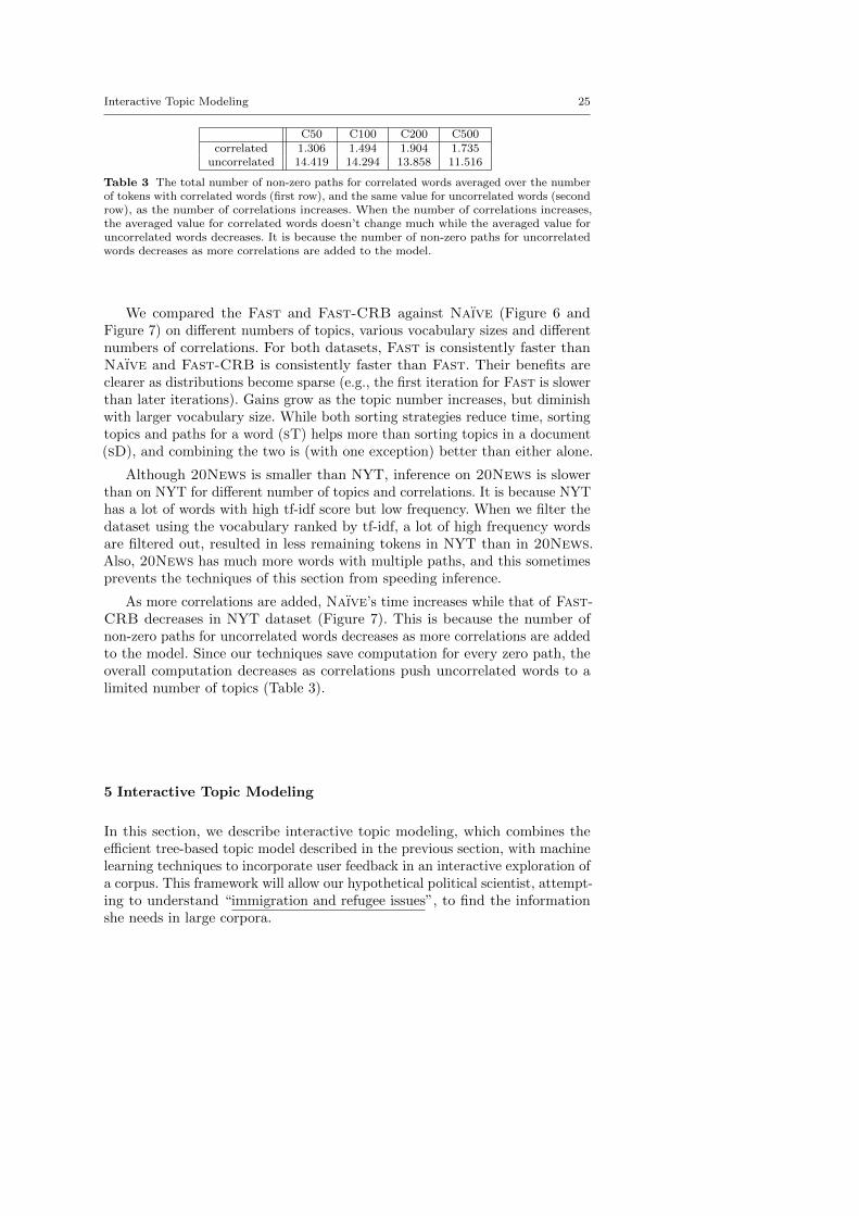
Table 3 The total number of non-zero paths for correlated words averaged over the numberof tokens with correlated words (first row), and the same value for uncorrelated words (secondrow), as the number of correlations increases. When the number of correlations increases,the averaged value for correlated words doesn’t change much while the averaged value foruncorrelated words decreases. It is because the number of non-zero paths for uncorrelatedwords decreases as more correlations are added to the model.
We compared the Fast and Fast-CRB against Naıve (Figure 6 andFigure 7) on different numbers of topics, various vocabulary sizes and differentnumbers of correlations. For both datasets, Fast is consistently faster thanNaıve and Fast-CRB is consistently faster than Fast. Their benefits areclearer as distributions become sparse (e.g., the first iteration for Fast is slowerthan later iterations). Gains grow as the topic number increases, but diminishwith larger vocabulary size. While both sorting strategies reduce time, sortingtopics and paths for a word (sT) helps more than sorting topics in a document(sD), and combining the two is (with one exception) better than either alone.
Although 20News is smaller than NYT, inference on 20News is slowerthan on NYT for different number of topics and correlations. It is because NYThas a lot of words with high tf-idf score but low frequency. When we filter thedataset using the vocabulary ranked by tf-idf, a lot of high frequency wordsare filtered out, resulted in less remaining tokens in NYT than in 20News.Also, 20News has much more words with multiple paths, and this sometimesprevents the techniques of this section from speeding inference.
As more correlations are added, Naıve’s time increases while that of Fast-CRB decreases in NYT dataset (Figure 7). This is because the number ofnon-zero paths for uncorrelated words decreases as more correlations are addedto the model. Since our techniques save computation for every zero path, theoverall computation decreases as correlations push uncorrelated words to alimited number of topics (Table 3).
5 Interactive Topic Modeling
In this section, we describe interactive topic modeling, which combines theefficient tree-based topic model described in the previous section, with machinelearning techniques to incorporate user feedback in an interactive exploration ofa corpus. This framework will allow our hypothetical political scientist, attempt-ing to understand “immigration and refugee issues”, to find the informationshe needs in large corpora.
26 Hu, Boyd-Graber, Satinoff, and Smith
5.1 Making Topic Models Interactive
As we argued in Section 2, there is a need for interactive topic models. Tradi-tional topic models do not offer a way for non-experts to tweak the models,and those that do are “one off” interactions that preclude fine-grained adjust-ments and tweaks that solve users’ problems but leave the rest of the modelunmolested. This section proposes a framework for interactive topic refinement,interactive topic modeling (ITM).
Figure 8 shows the process at a high level. Start with vanilla LDA (withoutany correlations), show users topics, solicit feedback from users, encode thefeedback as correlations between words, and then do topic modeling with thecorresponding tree-based prior. This process can be repeated until users aresatisfied.
Topic Models with a prior structure
Topic 1
Start withsymmetric prior
Build tree prior structure
Incrementaltopic learning
Get feedback from users
Fig. 8 Interactive topic modeling: start with a vanilla LDA with symmetric prior, get theinitial topics. Then repeat the following process till users are satisfied: show users topics, getfeedback from users, encode the feedback into a tree prior, update topics with tree-basedLDA.
Since it takes some effort for users to understand the topics and figure outthe “good” topics and “bad” topics, to save users’ effort and time, ITM shouldbe smart enough to remember the “good” topics while improving the “bad”topics. In this section, we detail how interactively changing correlations can beaccommodated in ITM.
A central tool that we will use is the strategic unassignment of states, whichwe call ablation (distinct from feature ablation in supervised learning). Thestate of a Markov Chain in MCMC inference stores the topic assignment ofeach token. In the implementation of a Gibbs sampler, unassignment is doneby setting a token’s topic assignment to an invalid topic (e.g., -1, as we usehere) and decrementing any counts associated with that token.
Interactive Topic Modeling 27
The correlations created by users implicitly signal that the model putcertain words in the wrong place. In other models, this input is sometimesused to “fix”, i.e., deterministically hold constant topic assignments (Ramageet al, 2009). Instead, we change the underlying model, using the current topicassignments as a starting position for a new Markov chain with some statesstrategically unassigned. How much of the existing topic assignments we useleads to four different options, which are illustrated in Figure 9.
An equivalent (and equally important) way to think about how ablationworks is as technique to handle the inertia of inference. Inference schemesfor topic models can become caught in local optima (Section 2.3); because ofthe way topic models are used, users can often diagnose these local optima.Ablation allows the errors that trap inference in local optima to be forgotten,while retaining the unobjectionable parts of the model. Without ablation,inertia would keep inference trapped in a local optimum.
Fig. 9 Four different strategies for state ablation after the words “dog” and “bark” areadded to the correlation “leash”, “puppy” to make the correlation “dog”, “bark”, “leash”,“puppy”. The state is represented by showing the current topic assignment after each word(e.g. “leash” in the first document has topic 3, while “forest” in the third document has topic1). On the left are the assignments before words were added to correlations, and on the rightare the ablated assignments. Unassigned tokens are given the new topic assignment -1 andare highlighted in red.
All We could revoke all state assignments, essentially starting the samplerfrom scratch. This does not allow interactive refinement, as there is nothingto enforce that the new topics will be in any way consistent with the existingtopics. Once the topic assignments of all states are revoked, all counts will bezero, retaining no information about the state the user observed.
28 Hu, Boyd-Graber, Satinoff, and Smith
Doc Because topic models treat the document context as exchangeable, adocument is a natural context for partial state ablation. Thus if a user addsa set of words S to correlations, then we have reason to suspect that alldocuments containing any one of S may have incorrect topic assignments.This is reflected in the state of the sampler by performing the Unassign(Algorithm 3) operation for each token in any document containing a wordadded to a correlation. This is equivalent to the Gibbs2 sampler of Yao et al(2009) for incorporating new documents in a streaming context. Viewed in thislight, a user is using words to select documents that should be treated as “new”for this refined model.
Algorithm 3 Unassign(doc d, token w)
1: Get the topic of token w: k2: Decrement topic count: nk|d −−3: for path λ of w in previous prior tree do4: for edge e of path λ do5: Decrement edge count: ne|k −−6: Forget the topic of token w
Algorithm 4 Move(doc d, token w)
1: Get the topic of token w: k2: for path λ′ of w in previous prior tree do3: for edge e′ of path λ′ do4: Decrement edge count: ne′|k −−5: for path λ of w in current prior tree do6: for edge e of path λ do7: Increment edge count: ne|k + +
Term Another option is to perform ablation only on the topic assignments oftokens which have been added to a correlation. This applies the unassignmentoperation (Algorithm 3) only to tokens whose corresponding word appears inadded correlations (i.e. a subset of the Doc strategy). This makes it less likelythat other tokens in similar contexts will follow the words explicitly includedin the correlations to new topic assignments.
None The final option is to move words into correlations but keep the topicassignments fixed, as described in Algorithm 4. This is arguably the simplestoption, and in principle is sufficient, as the Markov chain should find a stationarydistribution regardless of the starting position. However, when we “move”a token’s count (Algorithm 4) for word that changes from uncorrelated tocorrelated, it is possible that there is a new ambiguity in the latent state: wemight not know the path. We could either merge the correlations to avoid thisproblem (as discussed in Section 3.3), restricting each token to a unique path,or sample a new path. These issues make this ablation scheme undesirable.
The Doc and Term ablation schemes can be both viewed as online infer-ence (Yao et al, 2009; Hoffman et al, 2010). Both of them view the correlatedwords or some documents as unseen documents and then use the previously seendocuments (corresponding to the part of the model a user was satisfied with)in conjunction with the modified model to infer the latent space on the “new”data. Regardless of what ablation scheme is used, after the state of the Markovchain is altered, the next step is to actually run inference forward, sampling
Interactive Topic Modeling 29
assignments for the unassigned tokens for the “first” time and changing thetopic assignment of previously assigned tokens. How many additional iterationsare required after adding correlations is a delicate tradeoff between interactivityand effectiveness, which we investigate further in Section 6.
The interactive topic modeling framework described here fulfills the require-ments laid out in Section 2: it is simple enough that untrained users can providefeedback and update topics; it is flexible enough to incorporate that feedbackinto the resulting models; and it is “smart” enough—through ablation—toretain the good topics while correcting the errors identified by users. Interactivetopic modeling could serve the goals of our hypothetical political scientist toexplore corpora to identify trends and topics of interest.
6 Experiments
In this section, we describe evaluations of our ITM system. First, we describefully automated experiments to help select how to build a system that canlearn and adapt from users’ input but also is responsive enough to be usable.This requires selecting ablation strategies and determining how long to runinference after ablation (Section 6.1).
Next, we perform an open-ended evaluation to explore what untrained usersdo when presented with an ITM system. We expose our system to users on acrowd-sourcing platform and explore users’ interactions, and investigate whatcorrelations users created and how these correlations were realized on a socialmedia corpus (Section 6.2).
Our final experiment simulates the running example of a political scientistattempting to find and understand “immigration and refugee issues” in a largelegislative corpus. We compare how users—armed with either ITM or vanillatopic models—use these to explore a legislative dataset to answer questionsabout immigration and other political policies.
6.1 Simulated Users
In this section, we use the 20 Newsgroup corpus (20News) introduced inSection 4.5. We use the default split for training and test set, and the top 5000words are used in the vocabulary.
Refining the topics with ITM is a process where users try to map theirtopics in mind with the topics from topic models. The topics in users’ mind, ismostly related the category information. For the 20News corpus, users mighthave some category information in mind, such as, “politics”, “economies”,“energy”, “technologies”, “entertainments”, “sports”, “arts”, etc. They mighthave some words associated with each category. For example, the words “gov-ernment”, “president” for “politics”, and “gas”, “oil” for “energy”. Probablyat the beginning the word list associated with each category is not complete,that is, they have limited number of words in mind, but they might come upwith more words for each category later.
30 Hu, Boyd-Graber, Satinoff, and Smith
This whole process can be simulated by ranking words in each categoryby their information gain (IG).10 We start with the words with high IG foreach category, and gradually consider more words according to the ranking tosimulate the whole process. We treat the words in each category as a positivecorrelation and add one more word each round to refine the topics.
Sorting words by information gains discovers words that should be correlatedwith a classification label. If we believe that vanilla LDA lacks these correlations(because of a deficiency of the model), topics that have these correlationsshould better represent the collection (as measured by classification accuracy).Intuitively, these words represent a user thinking of a concept they believe isin the collection (e.g., “Christianity”) and then attempting to think of wordsthey believe should be connected to that concept.
For the 20News dataset, we rank the top 200 words for each class by IG,and delete words associated with multiple labels to prevent correlations fordifferent labels from merging. The smallest class had 21 words remaining afterremoving duplicates (due to high overlaps of 125 overlapping words between“talk.religion.misc” and “soc.religion.christian”, and 110 overlapping words be-tween “talk.religion.misc” and “alt.atheism”), so the top 21 words for each classwere the ingredients for our simulated correlations. For example, for the class“soc.religion.christian,” the 21 correlated words include “catholic, scripture,resurrection, pope, sabbath, spiritual, pray, divine, doctrine, orthodox.” Wesimulate a user’s ITM session by adding a word to each of the 20 positivecorrelations until each of the correlations has 21 words.
We evaluate the quality of the topic models through an extrinsic classifica-tion task. Where we represent a document’s features as the topic vector (themultinomial distribution θ in Section 3) and learn a mapping to one of thetwenty newsgroups using a supervised classifier (Hall et al, 2009). As the topicsform a better lower-dimensional representation of the corpus, the classificationaccuracy improves.
Our goal is to understand the phenomena of ITM, not classification, sothe classification results are well below state of the art. However, addinginteractively selected topics to state of the art features (tf-idf unigrams) givesa relative error reduction of 5.1%, while adding topics from vanilla LDA givesa relative error reduction of 1.1%. Both measurements were obtained withouttuning or weighting features, so presumably better results are possible.
We set the number of topics to be the same as the number of categoriesand hope the topics can capture the categories as well as additional relatedinformation. While this is not a classification task, and it is not directlycomparable with state of the art classifiers like SVM, we expect it performsbetter than the Null baseline, which is proved by Figure 10 and Figure 11.
This experiment is structured as a series of rounds. Each round addsan additional correlation for each newsgroup (thus 20 per round). After acorrelation is added to the model, we ablate topic assignments according toone of the strategies described in Section 5.1, run inference for some number
10 Computed by Rainbow toolbox, http://www.cs.umass.edu/∼mccallum/bow/rainbow/
Interactive Topic Modeling 31
of iterations, extract the new estimate of the per-document topic distribution,learn a classifier on the training data, and apply that classifier to the test data.We do 21 rounds in total, and the following sections investigate the choiceof number of iterations and ablation strategy. The number of LDA topics isset to 20 to match the number of newsgroups. The hyperparameters for allexperiments are α = 0.1, β = 0.01 for uncorrelated words, β = 100 for positivecorrelations and β = 10−6 for negative correlations.
We start the process after only 100 iterations of inference using a vanilla LDAmodel. At 100 iterations, the chain has not converged, but such small numbersof iterations is a common practice for impatient users initially investigating adataset (Evans, 2013; Carbone, 2012).11 After observing initial topics, the userthen gradually updates the topics, allowing inference to continue.
Moreover, while the patterns shown in Figure 11 were broadly consistentwith larger numbers of iterations, such configurations sometimes had too muchinertia to escape from local extrema. More iterations make it harder for thecorrelations to influence the topic assignment, another reason to start withsmaller numbers of initial iterations.
Investigating Ablation Strategies
First, we investigate which ablation strategy best incorporates correlations.Figure 10 shows the classification accuracy of six different ablation strategiesfor each of 21 rounds. Each result is averaged over five different chains using 10additional iterations of Gibbs sampling per round (other numbers of iterationsare discussed in Section 6.1). As the number of words per correlation increases,the accuracy increases as models gain more information about the classes.
To evaluate whether our model works better, we first compare our modelagainst a baseline without any correlations. This is to test whether the cor-relations help or not. This baseline is called Null, and it runs inference fora comparable number of iterations for fair comparison. While Null sees nocorrelations, it serves as a lower baseline for the accuracy but shows the effectof additional inference. Figure 10 shows that the Null strategy has a loweraccuracy than interactive versions, especially with more correlations.
We also compare our model with non-interactive baselines, which are AllInitial and All Full with all correlations known a priori. All Initial runsthe model for the only the initial number of iterations (100 iterations inthis experiment), while All Full runs the model for the total number ofiterations added for the interactive version. (That is, if there were 21 roundsand each round of interactive modeling added 10 iterations, All Full wouldhave 210 iterations more than All Initial). All Full is an upper baseline forthe accuracy since it both sees the correlations at the beginning and also runsfor the maximum number of total iterations. All Initial sees the correlationsbefore the other ablation techniques but it has fewer total iterations.
11 A machine learning purist would argue that such usage is incorrect, as you only wantsamples from a converged Markov chain. Without commenting on this debate, this experimentreflects the reality of how topic models are used for analyzing text.
32 Hu, Boyd-Graber, Satinoff, and Smith
0.500
0.525
0.550
0.575
0.600
0 5 10 15 20Rounds
Acc
urac
yStrategy
All Full
All Initial
Doc
None
Null
Term
Fig. 10 Accuracy (y-axis) using different ablation strategies as additional correlations areadded (x-axis). We start with 100 iterations, then for each round, add one more word for eachof the 20 positive correlations, and run 10 additional iterations. Null represents standardLDA, as the lower baseline. All Initial and All Full are non-interactive baselines, and AllFull is the upper baseline. The results of None, Term, Doc are more stable (as denotedby the bars), and the accuracy is increased gradually as more correlated words are added.
In Figure 10, both All Initial and All Full show a larger variance (asdenoted by bands around the average trends) than the interactive schemes.This can be viewed as akin to simulated annealing, as the interactive settingshave more freedom to explore in early rounds. For topic models with Docor Term ablation, this freedom is limited to only correlated words or wordsrelated with correlated words. Since the model is less free to explore the entirespace, these ablation strategies result in much lower variance.
All Full has the highest accuracy; this is equivalent to where users know allcorrelations a priori. This strategy corresponds to an omniscient and infinitelypatient user. Neither of these properties are realistic. First, it is hard for usersto identify and fix all problems at once. Often smaller problems are not visibleuntil larger problems have been corrected. This requires multiple iterations ofinspection and correction. Second, this process requires a much longer waitingtime, as all inference must be rerun from scratch after every iteration.
The accuracy of each interactive ablation strategy is (as expected) betweenthe lower and upper baselines. Generally, the correlations will influence notonly the topics of the correlated words, but also the topics of the correlatedwords’ context in the same document. Doc ablation gives more freedom forthe correlations to overcome the inertia of the old topic distribution and movetowards a new one influenced by the correlations.
How Many Iterations do Users Have to Wait?
For a fixed corpus and computational environment, the number of iterationsis the primary factor that determines how long a user has to wait. While more
Fig. 11 Classification accuracy by strategy and number of iterations between rounds. Westart with 100 iterations, then for each round, add one more word for each of the 20 positivecorrelations, and run additional 10 iterations. The Doc ablation strategy performs best,suggesting that the document context is important for ablation correlations. While moreiterations are better, there is a tradeoff with interactivity.
iterations can get closer to convergence, it also implies longer waiting time. Sowe need to balance convergence and waiting time.
Figure 11 shows the effect of using different numbers of Gibbs sampling iter-ations between rounds. For each of the ablation strategies, we run 10, 20, 30, 50,100 additional Gibbs sampling iterations. As expected, more iterations increaseaccuracy, although improvements diminish beyond 100 iterations. With morecorrelations, additional iterations help less, as the model has more a prioriknowledge to draw upon.
For all numbers of additional iterations, while the Null serves as the lowerbaseline for accuracy in all cases, the Doc ablation clearly outperforms theother ablation schemes, consistently yielding a higher accuracy. Thus, there isa benefit when the model has a chance to relearn the document context whencorrelations are added, and Doc provides the flexibility for topic models toovercome the inertia of the old topic distribution but does not throw awaythe old distribution entirely. The difference is greater with more iterations,suggesting Doc needs more iterations to “recover” from unassignment.
The number of additional iterations per round is directly related to users’waiting time. According to Figure 11, more iterations for each round achieveshigher accuracy, while increasing wait time. This is a tradeoff between latencyand model quality, and may vary based on users, applications, and data.
However, the luxury of having hundreds or thousands of additional iterationsfor each correlation would be impractical. For even moderately sized datasets,even one iteration per second can tax the patience of individuals who wantto use the system interactively. Studies have shown that a long waiting timemay affect cognitive load, making it harder for a user to recall what they weredoing or the context of the initial task (Ceaparu et al, 2004). Based on theseresults and an ad hoc qualitative examination of the resulting topics, we foundthat 30 additional iterations of inference was acceptable; this is used in laterexperiments, though this number can vary in different settings.
34 Hu, Boyd-Graber, Satinoff, and Smith
Fig. 12 Interface for Mechanical Turk experiments. Users see the topics discovered by themodel and select words (by clicking on them) to build correlations to be added to the model.
6.2 Users in Loop
To move beyond using simulated users adding the same words regardless ofwhat topics were discovered by the model, we needed to expose the model tohuman users. We solicited approximately 200 judgments from Mechanical Turk,a popular crowd-sourcing platform that has been used to gather linguisticannotations (Snow et al, 2008), measure topic quality (Chang et al, 2009;Stevens et al, 2012), and supplement traditional inference techniques for topicmodels (Chang, 2010). After presenting our interface for collecting judgments,we examine the results from these ITM sessions both quantitatively andqualitatively.
Figure 12 shows the interface used in the Mechanical Turk tests. The leftside of the screen shows the current topics in a scrollable list, with the top 30words displayed for each topic.
Users create correlations by clicking on words from the topic word lists.The word lists use a color-coding scheme to help the users keep track of whichwords they are already in correlations. The right side of the screen displaysthe existing correlations. Users can click on icons to edit or delete each one.The correlation being built is also shown in its own panel. Clicking on a wordwill remove that word from the current correlation.
Interactive Topic Modeling 35
0.427
0.571
0.662
0.682
1.00
1.02
1.04
0 1 2 3 4Round
Rel
ativ
e A
ccur
acy Topics
a
a
a
a
10 Topics
20 Topics
50 Topics
75 Topics
Fig. 13 The relative accuracy improvement (using round 0 as a baseline) of the bestMechanical Turk user session for each of the four numbers of topics, with the actual accuracymarked for the last round. While the 10-topic model does not provide enough flexibility tocreate good correlations, the best users could clearly improve classification with more topics.
Users were not given a specific goal; instead, they were instructed to addcorrelations between words so that the topics (we called them “word groups”in the instructions) made more sense. This was intentionally underspecified, aswe wanted to see what would happen when ITM was placed in the hands ofuntrained users.
As in Section 6.1, we can compute the classification accuracy for users asthey add words to correlations. The best users, who seemed to understand thetask well, were able to increase the classification accuracy (Figure 13). Themedian user, however, had an accuracy improvement indistinguishable fromzero. Despite this, we can examine the users’ behavior to better understandtheir goals and how they interact with the system.
The correlation sizes ranged from one word to over forty. The more words inthe correlation, the more likely it was to noticeably affect the topic distribution.This observation makes sense given our updating method. A correlation withmore words will probably cause the topic assignments to be reset for moredocuments.
Most of the large correlations (more than ten words) corresponded tothe themes of the individual newsgroups. Some common themes for largecorrelations were:
– Themes that matched a single newsgroup: religion, space exploration, health,foreign countries, cars, motorcycles, graphics, encryption
– Themes that spanned multiple related newsgroups: sports, government,computers, cars/motorcycles
– Themes that probably matched a sub-topic of a single newsgroup: homo-sexuality, Israel, computer programming
Some users created correlations with both “baseball” and “hockey” words,while others separated them. (“baseball” and “hockey” are in separate news-groups.) The separate correlations often contained overlapping words. Evenso, the choice of combined vs. separate correlations almost always determined
36 Hu, Boyd-Graber, Satinoff, and Smith
whether baseball and hockey would be in the same topic in the model. Asimilar situation occurred with “cars” and “motorcycles”, which are discussedin separate newsgroups.
Some users created inscrutable correlations, like “better”, “people”, “right”,“take”, “things” and “fbi”, “let”, “says”. They may have just clicked randomwords to finish the task quickly. While subsequent users could delete poorcorrelations, most chose not to. Because we wanted to understand broaderbehavior we made no effort to squelch such responses.
The two-word correlations illustrate an interesting contrast. Some pairs arelinked together in the corpus, like “jesus”, “christ”, “solar”, “sun”. Withothers, like “even”, “number” and “book”, “list”, the users seem to beencouraging collocations to be in the same topic. However, the collocationsmay not be present in any document in this corpus.
Not all sensible correlations led to successful topic changes. Many usersgrouped “mac” and “windows” together, but they were almost never placed inthe same topic. The corpus includes separate newsgroups for Macintosh andWindows hardware, and divergent contexts of “mac” and “windows” overpow-ered the prior distribution.
Other correlations led to topic changes that were not necessarily meaningful.For example, one user created a correlation consisting of male first names. Atopic did emerge with these words, but the rest of the words in that topicseemed random. This suggests that the set of male first names aren’t associatedwith each other in the corpus. Preliminary experiments on newspaper articleshad similar correlations that created a more meaningful topic associated withobituaries and social announcements.
Finally, many correlations depend on a user’s background and perspective,showing the flexibility of this approach. Some users grouped “israeli”, “jewish”,“arab”, and “muslim” with international politics words, and others with religionwords. On the other hand, “christian” was always grouped with religion words.The word “msg” appears to have two different interpretations. Some usersgrouped it with computer words (reading it as a message), while others groupedit with health words (reading it as a food additive).
As mentioned in Section 3, topic models with a tree-based prior can representsituations where words have multiple meanings. In previous work, the paths inthe tree—provided by WordNet—correspond to the distinct meanings of aword (Boyd-Graber et al, 2007). Users found the formalism intuitive enoughto build their own small WordNets to distinguish the different meanings of“msg”.
6.3 User Study
New systems for information access are typically investigated through task-based user studies to determine whether the new approach allows users tocomplete specific tasks as well as with current systems. Wacholder and Liu(2008), for example, compared traditional paper-based book indices with full-
Interactive Topic Modeling 37
text search for answering questions in large text collections. Following theirlead, we compare the information-seeking effectiveness using both interactiveand non-interactive topic modeling.
We asked users to fill the role of the running example a political scien-tist attempting to find legislation relevant to “immigration and refugee issues”(among other topics). Using full-text search aided by either vanilla topic modelsor interactive topic models (ITM), users were asked to answer questions basedcontent in a collection of legislative debates.
We found that users were able to answer the questions equally well in bothgroup with ITM (experimental group) and group without ITM (control group).However, users in the group using ITM had radically different strategies forhow they found information in the corpus. Rather than relying on full-textsearch, users used topic models to find relevant information.
6.3.1 Legislative Corpus
In the process of becoming a law, potential US legislation is sponsored by acongressperson and introduced for debate by a committee in either the USHouse of Representatives (lower chamber) or the US Senate (upper chamber).Once introduced, the bill is debated within the chamber it was introduced.Our corpus contains transcripts of these debates for the 109th congress, whichserved during the 2005 and 2006 calendar years.
The corpus is available online from GovTrack.12 Each page is associatedwith a bill and a vote. Uninteresting procedural bills, with less than 20% “Yea”votes or less than 20% “Nay” votes, are removed. We selected a subset ofthis congressional debate dataset that includes ten bills and their associateddebates. Each debate has multiple turns (a single uninterrupted speech by aunique congressperson), and we use each turn as a document for topic modeling.This yields 2,550 documents in total; we ignore all temporal, speaker-related,or legislative organization. While this is somewhat unrealistic for a real-worldstudy of legislative information, we will use some of this discarded informationto aid evaluation. The subset includes bills on immigration, the estate (death)tax, stem cell research, and others. Detailed information can be found inAppendix A.
6.3.2 Introduction of ITM Interface
The ITM interface is a web-based application.13 It provides a workflow forusers to select model parameters (corpus and number of topics), create aninitial topic model, name the topics, and refine the topics using ITM. Theinterface also provides multiple ways for a user to explore the corpus: a full-textsearch over all documents, a full-text search within a single topic, a listing of
12 http://www.govtrack.us/data/us/109/13 This ITM interface is with a HTML and jQuery ( http://jquery.com/ ) front end,
connected via Ajax and JSON
38 Hu, Boyd-Graber, Satinoff, and Smith
Fig. 14 The start page of ITM interface: users specify the user name, session name, corpus,number of topics, and experimental group (Group A: control group (LDA only); Group B:experimental group (ITM). )
documents associated with each topic, and links to access specific documents.We walk through this workflow in detail below.
From the initial screen (Figure 14), users specify the session information,such as user name, corpus, number of topics, etc. Once users click “start”,the interface loads the initial set of topics, including the top topic words andrelated documents, as shown in Figure 15. The top topic words are displayedsuch that the size of a word is proportional to the probability of this wordappearing in the topic.
After clicking on the topic, users can view additional information and, mostimportantly, edit the topic (editing is disabled for the control group). Afterclicking on a topic, three “bins” are visible: all, ignore, important. Initially, allof the topic words are in the “all” bin. As shown in Figure 16, users can dragwords to different bins based on their importance to the topic: words that areimportant to the topic to the“important” bin, words that should be ignoredin this topic to the “ignored” bin, and words that should be stopwords in thewhole corpus to “trash”. Users can also add new words to this topic by typingthe word and clicking “add”.14
Once the user has finished editing a topic, changes are committed bypressing the “Save” button. The backend then receives the users’ feedback. Themodel adds a positive correlation between all words in the “important” bin, anegative correlation between words in “ignored” bin and words in “important”bin, and removes words in the “trash” from the model. With these changesto the model, the ITM relearns the topics and updates the topics. While inprinciple users may update the topics as many times as they wish, our study
14 Only words present in the model’s vocabulary can be added; this constraint is enforcedvia an autocomplete function.
Interactive Topic Modeling 39
Fig. 15 Two topics displayed in the ITM interface. The most probable words in each topicare displayed with the size proportional to the probability of a word appearing in this topic.The documents most associated with each topic are shown in each topic’s panel. The usercan view all documents by selecting “view all documents”.
Rename your topic here
Type new words here
Limited by vocabulary
Display document (drag up and down to the context)
Fig. 16 ITM interface for refining a topic. Users can put words into different “bins”, nametopics, and add new words to the topic.
limited a user’s exploration and modification of topics to fifteen minutes. Then,the users entered the next phase of the study, answering questions about thecorpus.
In the question answering phase (Figure 17), users have three options toexplore the data to answer the questions: by reading through related documentsassociated with a topic, searching through all of the documents through full-text search, or via a text search restricted to a single topic. The full-textsearch is important because it is a commonly used means of finding datawithin large corpora (Shneiderman et al, 1997) and because it has been usedin previous previous information-seeking studies (Wacholder and Liu, 2008).
40 Hu, Boyd-Graber, Satinoff, and Smith
Fig. 17 Test page of the ITM interface. Users will see one question each time, and theycan answer the question by, searching keywords globally, checking the related topics or topicdocuments, or narrowing query results down by topics, that is, after a global query, click atopic, and the query results will be filtered by the relevance to this topic, displayed belowthe topic you clicked. Click “Next question” to proceed, and users are not allowed to go backto previous questions.
15 Initial studies, where access to the data was restricted to only topic modelinformation, were too difficult. We expect users to use topics when they areuseful and use full-text search when topics are less useful in answering aquestion. After each question, users click “Next question” to proceed; userscannot return to previous questions.
6.3.3 User Population
To evaluate the effectiveness of ITM for information-seeking tasks, we comparethe performance of users in two groups: and experimental group (ITM) and acontrol group (vanilla LDA).
For the experimental group, users start with an initial set of topics andcan refine the topics using ITM for up to fifteen minutes. They then start thetest phase for thirty minutes. They are provided with the refined topics for useduring the test.
The control group also has access to the initial topics, but they cannotrefine the topics. They are given up to fifteen minutes to check the topics,rename the topics, and review documents associated with the topics. This isto avoid experimental differences caused by the experimental group benefitingfrom exploring the corpus rather than from interactive topic modeling. After
15 Some examples where the websites for accessing the legislative data have full-text search:http://thomas.loc.gov/home/LegislativeData.php?n=BillText; http://www.senate.gov/ page-layout/legislative/g three sections with teasers/legislative home.htm.
Interactive Topic Modeling 41
spending up to fifteen minutes exploring the corpus, the control group also hasthirty minutes to answer the test questions.
The study participants are randomly assigned to a group. Each participantviews a video explaining how to use the interface and do the test. During thestudy, the system logs the related information of each user. After the study,participants complete a survey on their educational/technical background andfamiliarity with legislation or topic models.
The study had twenty participants (ten for each group). All of the usersare fluent in English. Participants are either students pursuing a degree inComputer Science, Information Science, Linguistics, or working in a related field.A post-test user survey revealed that most users have little or no knowledgeabout congressional debates and that users have varied experience with topicmodels.
We designed ten free response questions by exploring this legislation corpus,including questions regarding legislation which deals with taxes, the US-Mexicoborder, and other issues. The full text of the questions appears in Appendix B.
6.3.4 User Study Analysis
We examined two aspects of the experiment: how well the experimental group’sfinal topics replicated ground-truth annotations (below, we refer to this metricas refine) and how well both the groups answered the questions (test).
Our experiment views the corpus as an unstructured text collection (a typicaluse case of topic models); however, each turn in the dataset is associated witha single bill. We can view this association as the true clustering of the dataset.We compare this clustering against the clustering produced by assigning eachdocument to a cluster corresponding to its highest-probability topic.
We compare these reference clusters to the clusters produced by ITM usingvariation of information (Meila, 2007). This score has a range from zeroto infinity and represents the information-theoretic “distance” between twopartitions (lower is better). Using this information, we compute the variationof information (Meila, 2007) between the true labels and the topic modelingclusters. While we have a good initial set of topics (the initial variation ofinformation score is low), users in the experimental group—who claimed tohave little knowledge about the legislative process—still can reduce this scoreby refining the topics. To avoid bias from users, users do not know that theirtopics will be evaluated by variation of information.
As shown in Figure 18, ten users in the experimental group started withthe same initial topics and refined refine the topics for multiple rounds. Inthe given fifteen minutes, some users played with ITM for up to eight roundswhile one user only tried two rounds. Although users occasionally increasedthe variation of information, by the end of the refinement phase a majority ofusers successfully reduced the variation of information of the topics.
User “x2” provides an example of a successful ITM round. ’The user sawa topic mixing “energy”-related words with other words. To make a coherenttopic about “energy”, they put “oil”, “natural gas”, “gas”, “production” and
42 Hu, Boyd-Graber, Satinoff, and Smith
5.4
5.6
5.8
6.0
0 2 4 6 8number of rounds
varia
tion
of in
form
atio
n
new_id x0 x1 x11 x14 x15 x16 x19 x2 x6 x7
Fig. 18 Variation of information of users in experimental group at each round. Users arelabeled from x0 to x19. Ten of them are randomly assigned to experimental group. All tenusers start with the same initial topics and are able to refine the topics for the extent of therefinement phase. Most users in the experimental group successfully reduced the variation ofinformation (where lower is better).
“resources” in the important bin, and put “patriot act”, “federal government”,“tex cuts”, “stem cell” into the ignored bin. After updating, this topic be-came a coherent topic about “energy”. After refining topics for eight rounds,they successfully made other topics more coherent; he named these topics“homeland security”, “immigration”, “abortion”, “energy”, “flag burning”, etc.,which match well with the corpus’s true clusters. Thus this user successfullyreduced the variation of information as shown in Figure 18.
In addition to evaluating the variation of information for the experimentalgroup, we also evaluated the users’ answers to content-specific questions. Whilethe difference between the groups’ performance was not statistically significant,ITM changed the usage pattern to favor topic models over full text search.
To evaluate the test, we graded the answers and compared the scores ofusers in two groups. Of the 20 participants, two didn’t use their session namecorrectly, meaning the interface didn’t store their answers properly, and oneuser encountered an issue and wasn’t able to finish the questions. Thus wehave complete answers for 17 participants. Each question was graded by twograders with Scott’s π agreement 0.839 (Artstein and Poesio, 2005). Whilethere is no significant difference between the two groups’ test scores, the scoresfor experimental group had a much smaller variance compared to the controlgroup.
To better understand how users answer the questions, the ITM system logsthe number of full-text searches that include words from any of the topics(queried-topic-words) and the number of times that users used topics to filterquery results (query-in-topic).
The process of modifying topics inspired users in the experimental groupto use queries that included words from the topics (Figure 19); this may bebecause users learned more key terms while exploring and refining the topics.These topic words are helpful to answer questions: users in experimental group
Interactive Topic Modeling 43
0
10
20
30
40
queried−topic−words query−in−topicstatistics type
num
ber
of ti
mes
group control experimental
Fig. 19 Statistics show that users’ search strategies during the user study used topics morethan the control group.
queried topic words an average of 27.8 times, while the control group queriedtopic words 18.2 times on average. Users in the experimental group also used“query-in-topic” (restricting a full text search within a topic) more than the usersin control group. This is probably because those users working with refinedtopics that are better aligned with the underlying bills (several questions wereabout specific bills).
We also found that users in both groups click topics much more whenthe question is about the general understanding of the data set, for example,“Name 5 of the debated legislation in this data set.”. For more detailed questionslike “The Gulf of Energy Security act will provide revenue streams for whichfund?”, users in both groups prefer to use text query directly.
However, Figure 19 shows a large variance, so we should not overstate theseresults. In the conclusion, we discuss additional studies that can untangle theusefulness of topic models for evaluating information-seeking from other effectssuch as how familiar users are to topic models, whether they understand thetask clearly, and whether they are effective consumers of information.
Some users in the control group also performed very well. For example,user “x5” in the control group obtained a high score. During the initial fifteenminute exploration phase, this user clicked on topics to review documents 71times, substantially more than any user in either the control group or theexperimental group. Users such as “x5”, who are topic model-savvy have betterintuitions about how topic models work and how they can be used to helpexplore a corpus. In the post-session survey, the user reported that the interface,designed to facilitate ITM (but disabled for the control group) helped themunderstand the corpus and answer the questions.
Not all users in the experimental group performed well on the task. One useronly refined two topics, and some users failed to improve the topics (failed toreduce the variation of information). Some users complained that they weren’tgiven enough time to update the topics.
In general, most reported liking the interface. Users from both the experi-mental group and the control group commented that the topics helped themanswer some of the questions. Some users also commented that some of the
44 Hu, Boyd-Graber, Satinoff, and Smith
questions were too detailed, suggesting that perhaps additional methods tosearch the corpus may be helpful.
This study provides evidence that the ITM interface assists users in exploringa large corpus and that topic modeling is helpful for users attempting tounderstand legislative documents. Users used ITM to improve the initialclusters; this is especially promising, as these users had little backgroundknowledge of congressional debates and few had familiarity with topic models.
7 Automatically Suggesting Correlations
While we have demonstrated that ITM can encode correlations into topic modelsinteractively, our pilot with users showed that it is often difficult, particularlyfor untrained users, to decide how to guide interactive topic models. This isbecause there are many possible choices: if the vocabulary size is V , there areabout V 2 possible pair correlations (let alone higher order correlations). Inthis section, we build on heuristics proposed for topic coherence to suggestcorrelations automatically.
7.1 Generating New Correlations
Newman et al (2010) argues that topics whose words often appear close togetherin a reference corpus make more sense to users. They measure this throughpointwise mutual information (PMI) averaged over all word pairs present inthe top words of a topic (sorted in order of decreasing probability, as is usuallydone to show topics to a user). Thus, for a topic’s top words T ,
PMIC(T ) ≡∑
(wi,wj):wi 6=wj PMIC(wi, wj)
|T |(|T | − 1), (14)
where C is the corpus to compute PMI, and PMI is computed within a smalllocal window. Topics that have a high score tend to be judged as “makingsense” to users, and those that have lower scores tend to be judged as notmaking sense to users.
Based on this strategy, ITM could seek to improve this score by suggestingpositive correlations for pairs with high PMI score and negative correlationsfor pairs with low PMI score. To ensure that we only suggest meaningfulcorrelations, we weight suggestions by the tf-idf (Salton, 1968) for each word(by taking the max over all documents). This focuses correlations toward pairsthat are highly relevant to at least some subset of the documents (this preventscorrelations capturing syntactic or other dependencies). Combining the PMIand tf-idf score, we rank word pairs by
Fig. 20 The total number of votes across rounds for each topic by users on MechanicalTurk (16 votes for each topic). x-axis is in a decreasing order of the number of votes for ITM.The red colored topics are significantly different from a uniform vote distribution, whilethe others are not (tested by χ2-test). In general, there is no clear preference from usersbetween models with correlations (ITM) and models without (LDA), which is the result inimbalanced attention being focused on some topics more than others.
for positive correlations and by
NC(X,Y ) =maxd(tf-idf(X, d)) ·maxd(tf-idf(Y, d))
PMIC(X,Y )(16)
for negative correlations (NC). The pairs with the highest scores for thesemetrics become the suggestions. Since the number of word pairs is very large,we only consider the word pairs from different topics for PC and the word pairsfrom the same topic for NC.
Although we have an automatic technique for selecting correlations, thisdoes not replace a fully interactive system. This is because PMI ignores wordswith multiple meanings (e.g., “msg” in Section 6.2) and user-specific informationneeds (e.g., the examples in Section 2).
7.2 Human Evaluation over Automatically Generated Correlations
We use the 20 Newsgroups corpus (20News, described in Section 4.5) in thisexperiment. The topic number is set to be 20, and 100 iterations produce initialtopics. Four rounds of interaction are performed with 50 iterations each round.
In this experiment, we have two different topic models: one uses automati-cally generated correlations based on PMI20news (five positive and five negativecorrelations each round) and the other group runs for same number of iterationswithout any correlations. We name the two models as correlation group (ITM)and non-correlation group (LDA), respectively.
For evaluation, we showed the resulting topics to users on Mechanical Turkand asked whether they preferred the correlated topics (ITM), the controltopics (LDA), or they looked equally coherent (Equal). Four users comparedeach pair. The positioning (i.e., left vs. right) and order of words within a topicwere shuffled to avoid bias.
46 Hu, Boyd-Graber, Satinoff, and Smith
We first compared the votes for each group in each topic, as shown inFigure 20, in decreasing order of the number of votes for the correlated group(ITM). Users show significant preference in five of the total 20 topics (coloredin red, by χ2-test). Users did not have a clear preference overall; this wascounter-intuitive, as the correlations were changing the topics dramatically.There were three reasons that the correlations did not always favor the ITMgroup:
– first, topics that are most confusing (as measured by Equation 15 and 16)get the correlations to improve coherence; thus the correlations affect sometopics more than others
– second, because some topics have more correlations, other topics have fewercorrelations; thus those topics are similar to the uncorrelated case
– finally, some topics are ignored by correlations and have side-effects ofcorrelations in the other topics; these are not always good for the coherenceof the ignored topics
We describe each of these scenarios with examples, below.
Confusing Topic Gets the Correlations Some topics did show substantialimprovement, however. For example, Figure 21 shows how Topic 7 changes ascorrelations are added (we only show the correlations related with Topic 7).Initially, the topic mixes “transportation” and “health”, in the first round, anegative correlation between “car” and “cancer” pushed “car” away. Though“cars” remained, additional relevant terms—“medicine”, “pain”, “aids” and“effects” appeared. In the second round, when a negative correlation between“cancer” and “msg” was added, “cars” disappeared and most words in correlatedgroup (ITM) were related with “health”. The non-correlated group (LDA) alsostabilizes but much more slowly than the correlated group (ITM); after thefourth round, however, users do not have a clear preference.
Ignored Topics Stay the Same While Topic 7 was improved, Topic 5, initiallyincluding words “software, data, set, graphics, code, used, sun, user, following,text” etc., seemed the same for users’ observing the LDA and ITM versions ofthe topic, as shown in Table 4. In the second round of Topic 5, one positivecorrelation “window”, “widget” was added in ITM, but LDA already hadthese two correlated words in its topic, so the correlation had little effect onthe topic. In next round, two related negative correlations “max”, “font”and “max”, “window” were added to ITM, which improved the topic, sousers prefer the ITM. In first and last round, users have no preference betweenthe two groups.
Ignored Topics Suffer Side-effects Another case is that users sometimes deci-sively prefer the non-correlated group (LDA). For example, Topic 19, startedwith words “system, good, power, much, research, first, large, data, systems,work” etc., only had one relevant correlation, a negative correlation “max”,“model” added in the last round. However, the result of correlations in previous
Interactive Topic Modeling 47
car article cars insurance engine may water oil msg miles food medical disease doctor cancer health medicine body cause
medical cancer may disease drug water foodhealth treatment msg article cause cars doctor
engine anyone oil car ford used
medicine pain dog people aids effects
LDASPLIT
car, cancerITM
medicine doctor medical people disease drug food health treatment cause article msg water may
used cancer carford long much
body pain dog aidsresearch study
medicine medical cancer doctor food pain people disease drug water health may treatment aids msg article cause study
used could
researchblood
MERGEcancer, aidsmedical, cancercancer, medicine
body cancer doctor food medicine medical disease drug health water may vitamin treatment aids msg article cause study
painpeople
usedresearch
Round 1
LDA SPLIT cancer, msgITM
Round 2
LDA ITM
Round 3
Round 4
LDA ITM
Fig. 21 Compare the “evolution” of Topic 7 between LDA and ITM for four rounds: thecorrelations related with this topic is shown and we compared the topic words between LDAand ITM. At the beginning, Topic 7 is a mixed topic between “transportation” (blue) and“health” (red). While adding more correlations and running for additional iterations, thistopic becomes a pure “health” topic. While after four rounds, LDA and ITM got similarresult, ITM successfully made it the topic converge to a good coherent topic much faster.
rounds negatively impacted Topic 19, which had words “stolen” from it byother topics. This shows that improving some topics (e.g., Topic 7) sometimescomes at the expense of others; Table 4 shows that users preferred the versionof the topic left untouched by correlations.
Table 4 The round votes for Topic 5 and Topic 19. For Topic 5, while users have nopreference in R1 and R4, they prefer LDA in R2: one correlation “MERGE window, widget”was added in ITM, but LDA also had the two correlated words in its topic, so there was noclear improvement; in R3, two related correlations (“SPLIT max, font” and “SPLIT max,window”) were added to ITM, and users prefer the improved topic in ITM. For Topic 19, norelated correlations were added to ITM in the first three rounds; there was one unimportantcorrelation “SPLIT max, model” added in R4, which resulted in no clear improvement. Sousers clearly prefer LDA for Topic 19.
Figure 21 shows that for LDA and ITM, Topic 7 converged to the sametopic clear “health” topic, but ITM helped it converge the faster. We discuss
48 Hu, Boyd-Graber, Satinoff, and Smith
the distinction between improvements and impatience in Section 2.3, which alsogives an example of a topic that remains problematic even in a fully convergedtopic model.
8 Conclusion
Interactive topic modeling is a new framework for using and understandingstatistical models that empowers users of topic models to evaluate and refinetopics based on their unique expertise and perspective. These models offer newopportunities for wider and richer use of topic models, suggest new probabilisticmodels and methods for machine learning, and can serve as an exemplar forallowing users to improve statistical models.
Wider and Richer Uses of Topic Models
Topic models have attracted interest from not only the machine learningexperts, but also non-machine-learning experts in various fields includingcomputational social science (Lazer et al, 2009; Grimmer, 2010; Yang et al,2011), history (Hall et al, 2008; Mimno et al, 2012), psychology (Landauer et al,2006; Griffiths et al, 2007), biology (Ahmed et al, 2009; Ye et al, 2011), andmusic (Hu and Saul, 2009). These researchers have been able to understand,explain, and illustrate data that were, by virtue of their size, inaccessible for a“deep reading”. Study of these data are only possible using technology such astopic models.
But these investigations could be so much richer if this process were nota one-way experience. The adoption of topic models by broader communitiesrepresents an exciting opportunity for topic models to learn from researchers(usually, it’s the other way around). This would have manifold benefits: modelswould reflect expert knowledge, models would be less frustrating and more mal-leable, and different models could reflect disagreements or different perspectivesof model curators.
In addition to facilitating a richer experience for experts, interactive topicmodels offer an opportunity to better engage novices. Even though topic modelshave generated substantial interest from researchers outside machine learning,they remain less than user-friendly. Interactive models do not require users tobe machine learning experts to improve and adjust models; this can help usersslowly build statistical insights and facilitate greater uptake of computationalmethods in the social sciences.
Our future goal is to turn our running hypothetical political scientistinterested in understanding “immigration” into a reality. We are currentlyworking with political scientists to enable them to use topic models to discoverinteresting instances of where politicians have used loss or gain framing Tverskyand Kahneman (1992) to “spin” a topic to appeal to their core constituencies.Our user study showed that even novice users can use ITM to effectively explore
Interactive Topic Modeling 49
political corpora, and we expect better results from motivated researcherswilling to invest time understanding the ITM system.
However, the question of whether topic models assist users in informationseeking requires more experimentation. We showed that ITM encouraged usersto use topics to help them find information, but our population was too diverseand too small to be able to demonstrate that these techniques helped them tobetter or more quickly access the information.
Broadening the number of users for the user study would allow us to drawstronger conclusions about how interactive topic modeling changes or helpsthe way users seek out information from large corpora. In addition, with largerpopulations, a mixed-effects model could potentially untangle the effects ofhow familiar that users are to topic models, whether they understand thetask clearly, their background knowledge of the subject, and whether theyunderstand how to use the interface. Explicitly modeling and measuring theseeffects would effectively reduce the variance and help explain the interactionbetween these nuanced facets of user behavior.
New Probabilistic Models and Inference Techniques
In our attempt to minimize the latency a user could experience during theprocess of interactive topic modeling, we developed new techniques for proba-bilistic inference that take advantage of sparsity in probabilistic models. Whileour approach was more complicated than first method designed specifically forlatent Dirichlet allocation (Yao et al, 2009), it still offered substantial compu-tational speedup. This suggests that taking advantage of sparsity could alsobe used in other probabilistic models such as context-free grammars (Johnsonet al, 2007; Johnson, 2010) and feature-based models (Monroe et al, 2008; Wuet al, 2010).
While this work focused on text in a single language, tree based topicmodels have been used to explore multilingual corpora (Boyd-Graber andResnik, 2010; Jagarlamudi and Daume III, 2010), and from there it is a smallleap to multimodal data. Interactivity could be even more helpful in suchscenarios, as interaction in a user’s native language or in the most naturalmodality could help shape topics in the other language or modality. Forexample, an analyst trying to understand newspapers written in English andArabic might be more comfortable massaging the topics in English, but thosecorrelations would also improve the clustering for Arabic documents. Similarly,a topic-model clustering of image data with captions (Li Fei-Fei and Perona,2005) might be difficult to interact with visually, but suggesting correlationsbased on captions might lead to useful image clustering.
Toward More Interactive Statistical Models
While interactive topic modeling can obviate or replace some of the newertopic models, some models seem apt for interactive topic modeling. For example,combining interactivity with dynamic topic modeling (Blei and Lafferty, 2006;
50 Hu, Boyd-Graber, Satinoff, and Smith
Wang et al, 2008) could help to improve historians or social scientists workingwith datasets over long time periods; supervised topic models could helpresearchers understand how documents interact with external socioeconomicindicators such as the sentiment (Pang and Lee, 2008; Sayeed et al, 2012),consumer price index (Shoemaker, 2011), stock price (Bollen et al, 2010; Koganet al, 2009), or geography (Eisenstein et al, 2010); and topic models that gobeyond the bag of words (Wallach, 2006; Boyd-Graber and Blei, 2008) couldhelp understand syntactic patterns and linguistic structure.
Finally, the interactions that we observe from users could help us understandhow humans organize their mental vocabulary (Feldman et al, 2009). Insteadof just accepting user feedback as a given, we can explicitly model it usingtechniques such as Bayesian coalescents (Teh et al, 2008; Gorur and Teh, 2009).A joint model of both the tree structure and the topic model could learn users’desires and preferences from text; this would be a more statistically-drivenalternative to our approach of suggesting correlations and could help us learnmore from our users.
Learning from users is not just a benefit, but it is an essential goal formachine learning algorithms to be accepted by researchers who are not computerscientists and eventually the broader public. Interactive topic models are anexample of tools that can learn from and help users interact with large datasets,an essential tool for modern text-based research.
Acknowledgements We would like to thank Edmund Talley, Jonathan Chang, and PhilipResnik for their helpful comments. This work was supported by National Science Foundationgrant #0705832, Army Research Laboratory Cooperative Agreement W911NF-09-2-0072,and by National Science Foundation grant #1018625. Any opinions, findings, conclusions,or recommendations expressed are the authors’ and do not necessarily reflect those of thesponsors.
References
Abney S, Light M (1999) Hiding a semantic hierarchy in a Markov model. In:Proceedings of the Workshop on Unsupervised Learning in Natural LanguageProcessing, pp 1–8
Ahmed A, Xing EP, Cohen WW, Murphy RF (2009) Structured correspon-dence topic models for mining captioned figures in biological literature. In:International conference on Knowledge discovery and data mining, pp 39–48
Andrzejewski D, Zhu X, Craven M (2009) Incorporating domain knowledge intotopic modeling via Dirichlet forest priors. In: Proceedings of the InternationalConference of Machine Learning
Artstein R, Poesio M (2005) Kappa3 = alpha (or beta). Technical report,University of Essex Department of Computer Science
Astrachan O (2003) Bubble sort: an archaeological algorithmic analysis. In:Proceedings of the 34th SIGCSE technical symposium on Computer scienceeducation
Interactive Topic Modeling 51
Bendapudi N, Leone RP (2003) Psychological implications of customer partici-pation in co-production. Journal of Marketing 67(1):14–28
Blei DM, Lafferty JD (2005) Correlated topic models. In: Proceedings ofAdvances in Neural Information Processing Systems
Blei DM, Lafferty JD (2006) Dynamic topic models. In: Proceedings of theInternational Conference of Machine Learning
Blei DM, Ng A, Jordan M (2003) Latent Dirichlet allocation. Journal ofMachine Learning Research 3:993–1022
Blei DM, Griffiths TL, Jordan MI (2007) The nested Chinese restaurant processand hierarchical topic models. 0710.0845
Bollen J, Mao H, Zeng XJ (2010) Twitter mood predicts the stock market.CoRR abs/1010.3003
Boyd-Graber J, Blei DM (2008) Syntactic topic models. In: Proceedings ofAdvances in Neural Information Processing Systems
Boyd-Graber J, Resnik P (2010) Holistic sentiment analysis across languages:Multilingual supervised latent Dirichlet allocation. In: Proceedings of Em-perical Methods in Natural Language Processing
Boyd-Graber J, Blei DM, Zhu X (2007) A topic model for word sense dis-ambiguation. In: Proceedings of Emperical Methods in Natural LanguageProcessing
Boydstun AE, Glazier RA, Phillips C (2013) Agenda control in the 2008presidential debates. American Politics Research
Bron C, Kerbosch J (1973) Algorithm 457: finding all cliques of an undirectedgraph. Communications of the ACM 16(9):575–577
Carbone K (2012) Topic modeling: Confusion and excitement.Http://dh201.humanities.ucla.edu/?p=502
Ceaparu I, Lazar J, Bessiere K, Robinson J, Shneiderman B (2004) Determiningcauses and severity of end-user frustration. International journal of human-computer interaction 17(3):333–356
Chang J (2010) Not-so-latent Dirichlet allocation: Collapsed Gibbs sampling us-ing human judgments. In: NAACL Workshop: Creating Speech and LanguageData With Amazon’ss Mechanical Turk
Chang J, Boyd-Graber J, Wang C, Gerrish S, Blei DM (2009) Reading tealeaves: How humans interpret topic models. In: Proceedings of Advances inNeural Information Processing Systems
Daume III H (2009) Markov random topic fields. In: Proceedings of ArtificialIntelligence and Statistics
Dietz L, Bickel S, Scheffer T (2007) Unsupervised prediction of citation influ-ences. In: Proceedings of the International Conference of Machine Learning
Drouin J (2011) Foray into topic modeling. Ecclesiastical Proust ArchiveEisenstein J, O’Connor B, Smith NA, Xing EP (2010) A latent variable model
for geographic lexical variation. In: EMNLP’10, pp 1277–1287Evans P (2013) More fun with topic modeling.
Http://mith.umd.edu/engl668k/?p=1595Feldman NH, Griffiths TL, Morgan JL (2009) Learning phonetic categories
by learning a lexicon. In: Proceedings of the 31st Annual Conference of the
52 Hu, Boyd-Graber, Satinoff, and Smith
Cognitive Science SocietyGorur D, Teh YW (2009) An efficient sequential Monte Carlo algorithm for
coalescent clustering. In: Proceedings of Advances in Neural InformationProcessing Systems
Griffiths TL, Steyvers M (2004) Finding scientific topics. Proceedings of theNational Academy of Sciences 101(Suppl 1):5228–5235
Griffiths TL, Canini KR, Sanborn AN, Navarro DJ (2007) Unifying rationalmodels of categorization via the hierarchical Dirichlet process. In: Proceedingsof the 29th Annual Conference of the Cognitive Science Society
Grimmer J (2010) A bayesian hierarchical topic model for political texts:Measuring expressed agendas in senate press. Political Analysis
Gruber A, Rosen-Zvi M, Weiss Y (2007) Hidden topic Markov models. In:Artificial Intelligence and Statistics
Hall D, Jurafsky D, Manning CD (2008) Studying the history of ideas usingtopic models. In: Proceedings of Emperical Methods in Natural LanguageProcessing
Hall M, Frank E, Holmes G, Pfahringer B, Reutemann P, Witten IH (2009)The WEKA data mining software: An update. SIGKDD Explorations 11
Harary F (1969) Graph Theory. Addison-WesleyHeinrich G (2004) Parameter estimation for text analysis. Tech. rep.,
http://www.arbylon.net/publications/text-est.pdfHoffman M, Blei DM, Bach F (2010) Online learning for latent Dirichlet
allocation. In: NIPSHopcroft H, Tarjan R (1973) Algorithm 447: efficient algorithms for graph
manipulation. Communications of the ACM 16(6):372–378Hopkins DJ (2012) The exaggerated life of death panels: The limits of framing
effects in the 2009-2012 health care debateHu D, Saul LK (2009) A probabilistic model of unsupervised learning for
musical-key profiles. In: International Society for Music Information RetrievalConference
Hu Y, Boyd-Graber J (2012a) Efficient tree-based topic modeling. In: Associa-tion for Computational Linguistics
Hu Y, Boyd-Graber J (2012b) Suggesting constraints for interactive topicmodeling. In: ICML Workshop on Machine Learning in Human Computationand Crowdsourcing
Hu Y, Boyd-Graber J, Satinoff B (2011) Interactive topic modeling. In: Pro-ceedings of the Association for Computational Linguistics
Jagarlamudi J, Daume III H (2010) Extracting multilingual topics from un-aligned corpora. In: Proceedings of the European Conference on InformationRetrieval (ECIR), Milton Keynes, United Kingdom
Johnson M (2010) PCFGs, topic models, adaptor grammars and learningtopical collocations and the structure of proper names. In: Proceedings ofthe Association for Computational Linguistics
Johnson M, Griffiths TL, Goldwater S (2007) Bayesian inference for PCFGs viaMarkov chain Monte Carlo. In: Conference of the North American Chapterof the Association for Computational Linguistics
Interactive Topic Modeling 53
Kogan S, Levin D, Routledge BR, Sagi JS, Smith NA (2009) Predicting riskfrom financial reports with regression. In: Conference of the North AmericanChapter of the Association for Computational Linguistics
Lau JH, Grieser K, Newman D, Baldwin T (2011) Automatic labelling of topicmodels. In: Proceedings of the Association for Computational Linguistics,pp 1536–1545
Lavine M (1992) Some aspects of Polya tree distributions for statistical model-ing. The Annals of Statistics 20(3):1222–1235
Lazer D, Pentland A, Adamic L, Aral S, Barabasi AL, Brewer D, ChristakisN, Contractor N, Fowler J, Gutmann M, Jebara T, King G, Macy M, RoyD, Alstyne MV (2009) Social science: Computational social science. Science323(5915):721–723
Li W, Mccallum A (2006) Pachinko allocation: Dag-structured mixture modelsof topic correlations. In: International Conference on Machine Learning, pp577–584
Li Fei-Fei, Perona P (2005) A Bayesian hierarchical model for learning naturalscene categories. In: Computer Vision and Pattern Recognition, pp 524–531
Lin WH, Wilson T, Wiebe J, Hauptmann A (2006) Which side are you on?identifying perspectives at the document and sentence levels. In: Proceedingsof the Conference on Natural Language Learning (CoNLL)
Loper E, Bird S (2002) NLTK: the natural language toolkit. In: Tools andmethodologies for teaching
Meeks E (2011) Comprehending the digital humanities. Digital HumanitiesSpecialist
Meila M (2007) Comparing clusterings—an information based distance. Journalof Multivariate Analysis 98(5):873–895
Miller GA (1990) Nouns in WordNet: A lexical inheritance system. InternationalJournal of Lexicography 3(4):245–264
Mimno D, Wallach H, McCallum A (2008) Gibbs sampling for logistic normaltopic models with graph-based priors. In: NIPS 2008 Workshop on AnalyzingGraphs: Theory and Applications
Mimno D, Wallach H, Talley E, Leenders M, McCallum A (2011) Optimizingsemantic coherence in topic models. In: Proceedings of Emperical Methodsin Natural Language Processing
Mimno D, Hoffman M, Blei D (2012) Sparse stochastic inference for latentDirichlet allocation. In: Proceedings of the International Conference of Ma-chine Learning
Monroe BL, Colaresi MP, Quinn KM (2008) Fightin’ Words: Lexical FeatureSelection and Evaluation for Identifying the Content of Political Conflict.Political Analysis, Vol 16, Issue 4, pp 372-403, 2008
Nah FFH (2004) A study on tolerable waiting time: how long are web userswilling to wait? Behaviour & Information Technology 23(3):153–163
Neal RM (1993) Probabilistic inference using Markov chain Monte Carlomethods. Tech. Rep. CRG-TR-93-1, University of Toronto
54 Hu, Boyd-Graber, Satinoff, and Smith
Nelson RK (2010) Mining the dispatch. Http://dsl.richmond.edu/dispatch/Newman D, Karimi S, Cavedon L (2009) External evaluation of topic models.
In: Proceedings of the Aurstralasian Document Computing SymposiumNewman D, Lau JH, Grieser K, Baldwin T (2010) Automatic evaluation of topic
coherence. In: Conference of the North American Chapter of the Associationfor Computational Linguistics
Norman DA (ed) (1993) Things That Make Us Smart: Defending HumanAttributes In The Age Of The Machine. Addison-Wesley, Reading MA
Norman DA (2002) The Design of Everyday Things, reprint paperback edn.Basic Books
O Seaghdha D, Korhonen A (2012) Modelling selectional preferences in alexical hierarchy. In: Proceedings of the 1st Joint Conference on Lexical andComputational Semantics
Pang B, Lee L (2008) Opinion Mining and Sentiment Analysis. Now PublishersInc
Paul M, Girju R (2010) A two-dimensional topic-aspect model for discover-ing multi-faceted topics. In: Association for the Advancement of ArtificialIntelligence
Petterson J, Alex S, Caetano T, Buntine W, Shravan N (2010) Word featuresfor latent Dirichlet allocation. In: Neural Information Processing Systems
Ramage D, Hall D, Nallapati R, Manning C (2009) Labeled LDA: A supervisedtopic model for credit attribution in multi-labeled corpora. In: Proceedingsof Emperical Methods in Natural Language Processing
Resnik P, Hardisty E (2010) Gibbs sampling for the uninitiated. Tech. Rep.UMIACS-TR-2010-04, University of Maryland
Rosen-Zvi M, Griffiths TL, Steyvers M, Smyth P (2004) The author-topicmodel for authors and documents. In: Proceedings of Uncertainty in ArtificialIntelligence
Salton G (1968) Automatic Information Organization and Retrieval. McGrawHill Text
Sayeed AB, Boyd-Graber J, Rusk B, Weinberg A (2012) Grammatical struc-tures for word-level sentiment detection. In: North American Association ofComputational Linguistics
Shneiderman B, Byrd D, Croft WB (1997) Clarifying search: A user-interfaceframework for text searches. D-Lib Magazine 3(1)
Shoemaker OJ (2011) Variance estimates for price changes in the consumerprice index. Bureau of Labor Statistics Report
Shringarpure S, Xing EP (2008) mStruct: a new admixture model for inferenceof population structure in light of both genetic admixing and allele mutations.In: Proceedings of the International Conference of Machine Learning
Snow R, O’Connor B, Jurafsky D, Ng A (2008) Cheap and fast—but is itgood? Evaluating non-expert annotations for natural language tasks. In:Proceedings of Emperical Methods in Natural Language Processing
Stevens K, Kegelmeyer P, Andrzejewski D, Buttler D (2012) Exploring topiccoherence over many models and many topics. In: Empirical Methods inNatural Language Processing, vol 20
Interactive Topic Modeling 55
Talley EM, Newman D, Mimno D, Herr BW, Wallach HM, Burns GAPC,Leenders AGM, McCallum A (2011) Database of NIH grants using machine-learned categories and graphical clustering. Nature Methods 8(6):443–444
Teh YW, Jordan MI, Beal MJ, Blei DM (2006) Hierarchical Dirichlet processes.Journal of the American Statistical Association 101(476):1566–1581
Teh YW, Daume III H, Roy DM (2008) Bayesian agglomerative clustering withcoalescents. In: Proceedings of Advances in Neural Information ProcessingSystems
Templeton C (2011) Topic modeling in the humanities: An overview. MarylandInstitute for Technology in the Humanities Blog
Thomas JJ, Cook KA (2005) Illuminating the path: The research and develop-ment agenda for visual analytics. IEEE Computer Society Press
Tversky A, Kahneman D (1992) Advances in prospect theory: Cumulativerepresentation of uncertainty. Journal of Risk and Uncertainty 5(4):297–323
Wacholder N, Liu L (2008) Assessing term effectiveness in the interactive infor-mation access process. Information Processing and Management 44(3):1022–1031
Wallach HM (2006) Topic modeling: Beyond bag-of-words. In: Proceedings ofthe International Conference of Machine Learning
Wang C, Blei DM, Heckerman D (2008) Continuous time dynamic topic models.In: Proceedings of Uncertainty in Artificial Intelligence
Wei X, Croft B (2006) LDA-based document models for ad-hoc retrieval. In:Proceedings of the ACM SIGIR Conference on Research and Developmentin Information Retrieval
Wu X, Yu K, Wang H, Ding W (2010) Online streaming feature selection. In:International Conference on Machine Learning, pp 1159–1166
Yang TI, Torget A, Mihalcea R (2011) Topic modeling on historical newspapers.In: Proceedings of the 5th ACL-HLT Workshop on Language Technology forCultural Heritage, Social Sciences, and Humanities
Yao L, Mimno D, McCallum A (2009) Efficient methods for topic modelinference on streaming document collections. In: Knowledge Discovery andData Mining
Ye X, Yu YK, Altschul SF (2011) On the inference of Dirichlet mixture priors forprotein sequence comparison. Journal of Computational Biology 18:941–954
56 Hu, Boyd-Graber, Satinoff, and Smith
Appendix
Appendix A: Titles of the ten bills used in the user study (Section 6.3)
– H.R. 6061: Secure Fence Act of 2006– H.R. 8: Death Tax Repeal Permanency Act of 2005– S. 2271: USA PATRIOT Act Additional Reauthorizing Amendments Act
of 2006– S. 3711: Gulf of Mexico Energy Security Act of 2006– S. 3711: Gulf of Mexico Energy Security Act of 2006– S. 403: Child Custody Protection Act– H.R. 4297: Tax Increase Prevention and Reconciliation Act of 2005– S.J.Res. 12: Flag Desecration resolution– H.R. 810: Stem Cell Research Enhancement Act of 2005– H.R. 810: Stem Cell Research Enhancement Act of 2005
Appendix B: Questions list in the user study (Section 6.3)
– The flag desecration act gives power to what body to prohibit physicaldesecration of the flag of the United States?
– The child custody protection act makes it what type of crime to take minorsacross state lines to circumvent laws requiring involvement of parents inabortion decisions?
– According to the debate for the secure fence act, what is the length (inmiles) of the border that the U.S. shares with Mexico?
– The Gulf of Energy Security act will provide revenue streams for whichfund?
– A senator compares the immigration debate to the release of what film?– Name 5 of the debated legislation in this data set. Give either the full name
or the number assigned to the debate.– Name 2 of the debated legislation in this data set deals with taxes or the
budget?– What is the name of the debated legislation which proposes an amendment
to the constitution?– Name the 2 debated legislation in this data set that discusses illegal immi-