Zentrum fur TechnomathematikFachbereich 3 – Mathematik und Informatik

Quenching simulation for the inductionhardening process – Thermal and

mechanical effects

J. Montalvo-Urquizo Q. Liu A. Schmidt

Report 13–02

Berichte aus der Technomathematik

Report 13–02 May 2013

Quenching simulation for the induction hardening

process – Thermal and mechanical effects

J. Montalvo-Urquizoa,∗, Q. Liua, A. Schmidta

aZentrum fur Technomathematik, University of Bremen, Germany

Abstract

We investigate the mathematical model for induction hardening of steel andpresent simulation results for the involved cooling process. The model ac-counts for the thermomechanical effects coupled with phase transitions thatare caused by the enormous changes in temperature during the heat treat-ment. The mechanical part of the quenching model includes the transfor-mation strain and transformation plasticity induced by the phase transi-tions (TRIP). The simulations have been performed by assuming a non-homogeneous pre-heated workpiece with an austenite profile generated viahigh-frequency inductive heating. The mathematical ingredients of the modelare presented and the main simulation results are reported for the case of agearing component made of steel 42CrMo4.

Key words: Heat treatment, surface hardening, phase transitions,Transformation induced plasticity, Quenching

1. Introduction

For many applications in industry the surface of steel components is par-ticularly stressed. Therefore, there exists a growing demand of surface hard-ened products. Hardening is a metallurgical and metalworking process usedto increase the hardness of the boundary layers of a workpiece made of steel.The first step for hardening is the heating of the components to a temper-ature at which the iron phase changes from the initial phase into austenite.

∗Corresponding authorEmail addresses: montalvo@math.uni-bremen.de (J. Montalvo-Urquizo),

liu@math.uni-bremen.de (Q. Liu), schmidt@math.uni-bremen.de (A. Schmidt)

Preprint submitted to Berichte aus der Technomathematik May, 2013

Then the material is quenched by applying high cooling rates on it. The rea-son why the hardness of steel can be changed relies on the occurring phasetransitions. In the case of surface hardening, high cooling rates should beachieved so that most of the austenite phase is transformed to martensite bya diffusionless phase transition, producing the desired hardening effect.

Induction hardening is one of the most important surface hardening pro-cedures and has been successfully applied in industry for more than 50 years.In this heat treatment method, an induction coil is connected to the powersupply and the flow of alternating current through the coil generates analternating magnetic field which in turn induces eddy currents in the work-piece. The energy dissipated due to these currents causes heat in the steelcomponent and can be used to heat up only a specific part of it.

Although the inductive hardening is well established among practitioners,the needs for process optimization are still open. In this sense, the modeling,numerical simulation, and optimization remain areas of great interest in theapplied research.

In this paper, we report on the research performed for a subproject ofthe network MeFreSim–Modeling, Simulation and Optimization of Multi-Frequency Induction Hardening as Part of Modern Production formed bythe Weierstraß-Institut fur Angewandte Analysis und Stochastik (Berlin),the Zentrum fur Technomathematik (Universitat Bremen), the Institut furMathematik (Universitat Augsburg), the Stiftung Institut fur Werkstoff-stechnik (Bremen), and the industrial partners EFD Induction GmbH andZF Friedrichshafen AG.

We present here our work performed within the research network, con-sisting of the numerical simulation of thermomechanical effects due to thephase transitions during the quenching process of gear components.

This work deals with the model and simulation for the quenching pro-cess after a high-temperature profile has been achieved with an inductor ona gearing component. The rather general model for quenching of steel ispresented in Section 2, including heat conduction, phase transformations,thermoelasticity and transformation induced plasticity (TRIP) to be consid-ered in the computations. After this, Section 3 presents the material data,simulation setting and main results for an implementation of a gearing com-ponent made of steel 42CrMo4. The final Section 4 draws some concludingremarks and present some ideas for further research.

2

2. The mathematical model

For the complete heat treatment cycle we usually consider four character-istic times: the beginning of the heating process t0 (at room temperature),the end of the heating process t1, the end of a mantained high temperaturet1, and the end of the quenching process t2. In the case of induction hard-ening the stabilization period [t1, t1] is very small and can be neglected suchthat the process is only characterized by the heating interval [t0, t1) and thequenching interval [t1, t2].

At time t0 steel is assumed to consist of a mixture of ferrite, pearlite,bainite, and some martensite (the last one typically representing the smallestamount). Unfortunately the exact phase distribution of such mixture ofphases is unknown in practice and represents an uncertainty factor in themodel. For this reason we introduce the symbol Z0 which will be reserved inthe following for the initial phase mixture prior to the heat treatment. Duringthe heating process Z0 is (partially) transformed to austenite. Later, duringthe (rapid) cooling stage, the austenitic phase is transformed mainly intomarteniste, but it may also be transformed into ferrite, pearlite, and baintein a much smaller portion; the remaining volume fraction of Z0 remainsunchanged.

A good model for describing the heat treatment of steel is based on thethermal and mechanical equations for the description of temperature andmechanical deformations in the material pieces. Similar models with coupledequations for thermomechanical problems have been previously simulated forprocesses like heat treatment, welding and shape rolling, among others (cf.e.g. [1], [5], [12], [14]).

The rapid cooling rates are obtained by prescribing appropriate bound-ary conditions in a heat equation and the temperature gives rise to the timeevolution of the single phases. The coupling between the thermal and themechanical models is determined by the density changes in material resultingfrom temperature and phase changes, as well as by the mechanical dissipa-tion. At the same time, the phases’ evolution is a direct consequence of thetemperature changes, as described below.

2.1. The phase transitions

Mathematical models for phase transitions in steel have been considerede.g. in [4]–[6], [8], [14], [17], [18], [19]. In many works, the description of the

3

diffusive phase transitions in the isothermal case is done via the Johnson-Mehl equation. In order to establish a general model for isothermal multi-phase case during the cooling process we introduce the following notations:

• z0(t): the volume fraction of Z0, i.e., the mixture of phases presentbefore the heating process,

• z10 : the volume fraction of austenite at time t1 which stands for theend-time of the heating process (i.e. the start of quenching)

• z1(t): the volume fraction of remaining austenite during the coolingprocess, and,

• z2(t), · · · , z5(t): volume fraction of ferrite, pearlite, bainite, martensite,which have been transformed from austenite during cooling.

As mentioned, the workpiece has the phase configuration Z0 at time t0,thus we have z0(t0) = 1. Since the outer layers of the workpiece have beentransformed to austenite from Z0 during the heating process, it is observedthat the phases at the end of heating correspond to a portion of Z0 and aportion of austenite, it is z0(t1) + z1(t1) = 1.

During quenching, austenite is transformed into ferrite, pearlite, bainiteand marteniste, then we can conclude

z1(t1) ≡ z10 = z1(t) + z2(t) + z3(t) + z4(t) + z5(t) for t ∈ (t1, t2].

and the remaining fraction of Z0 remains unchanged during cooling andequals to z0(t1).

We describe the evolution of volume fractions during the cooling processwhich occurs for t ∈ [t1, t2] by the following equations

z2(t) + z3(t) = z10

(

1− e−b(θ)(t−t1)a(θ))

for FPf≤ θ ≤ FPs ,

z4(t) = (z10 − (z2(t) + z3(t)))(

1− e−b(θ)(t−t1)a(θ))

for Bf ≤ θ ≤ Bs,

z5(t) = (z10 − z2(t)− z3(t)− z4(t))

(

1−

(

θ −Mf

Ms −Mf

)n)

for Mf ≤ θ ≤Ms,

(1)where the evolutions of ferrite, pearlite and bainite (the first and the secondequations) arise from the Johnson-Mehl-Avrami equation and the austenite-marteniste phase change (the third equation) is from Schroder’s approach,

4

see e.g. [13]. The parameters b(θ), a(θ), b(θ), a(θ) and n have to be identifiedusing experimental data as in [11]. FPs(FPf

), Bs(Bf ), and Ms(Mf ) denotethe start (end) temperatures of formations of ferrite/pearlite, bainite andmartensite, respectively.

The equations (1) may be then be reduced to a system of ODEs. Forsimplicity, let z denote z2+z3, then it is easy to verify from the first equationin (1) that

t− t1 =

ln

(

1−z

z10

)

−b(θ)

1/a(θ)

. (2)

Formal differentiation of (2) with respect to time gives the ordinary differ-ential equation

˙z = −a(θ)b(θ)1/a(θ)(z10 − z)

(

ln

(

1−z

z10

))1−1

a(θ) . (3)

In a similar manner, using the second equation in (1) one gets

z4 = −a(θ)b(θ)1/a(θ)(z10 − z − z4)

(

ln

(

1−z4

z10 − z

))1−1

a(θ)−

z4 ˙z

z10 − z. (4)

and then the problem (1) is equivalent to the initial-value ODEs

˙z = −a(θ)b(θ)1/a(θ)(z10 − z)

(

ln

(

1−z

z10

))1−1

a(θ) H(θ − FPf)H(FPs − θ),

z4 =

−a(θ)b(θ)1/a(θ)(z10 − z − z4)

(

ln

(

1−z4

z10 − z

))1−1

a(θ)−

z4 ˙z

z10 − z

×

×H(θ −Bf )H(Bs − θ),

z5 =

(

d

dt

(

(z10 − z − z4)

(

1−

(

θ −Mf

Ms −Mf

)n)))

H(θ −Mf )H(Ms − θ),

z(t1) = z4(t1) = z5(t1) = 0,

(5)

where H denotes the heaviside step function.

5

2.2. Thermomechanical modelingWe assume small deformations and consider the balance law of momen-

tum without inertial term together with the balance of internal energy as

− div σ = 0, (6)

e+ div q = σ : ε(u) + h, (7)

which are essential to determine the displacement u, the stress tensor σ andthe temperature θ. Here is the mass density, q is the heat flux, e the specificinternal energy, ε(u) = 1

2(∇u +∇uT ) the symmetric part of the strain rate

tensor and h the external heat source. Further, we assume that the totalstrain ε(u) can be additively decomposed in an elastic part εel, a thermalpart εth, and a TRIP part εtrip (cf. [7] for details), i.e.

ε(u) = εel + εth + εtrip. (8)

We describe the thermal strain as the thermal expansion produced bydensity changes, it is

εth =

(

(

0(θref )

(θ, z)

)13

− 1

)

I.

where 0(θref ) stands for the homogenous measured density of the initialphase configuration z0(t0) at reference temperature θref and we make a mix-ture ansatz for the density as

(θ, z) =5∑

i=0

zii(θ), (9)

where i(θ) is the homogenous temperature-dependent density of the phasezi at temperature θ. Moreover the thermal part εth can be subsequentlydecomposed in an isothermal phase transition effect at reference temperatureθref and a thermal expansive part without phase transitions, i.e.

εth ≈

(

(

0(θref )

(θref , z)

)13

− 1

)

I +5∑

i=0

ziαi(θ)(θ − θref )I

≈ −1

3

(

(θref , z)

0(θref )− 1

)

I +5∑

i=0

ziαi(θ)(θ − θref )I

= −1

3

5∑

i=0

zi(

i(θref )

0(θref )− 1

)

I +5∑

i=0

ziαi(θ)(θ − θref )I,

(10)

6

here αi(θ) is the linear thermal expansion coefficient of the phase zi wherewe assume the density i(θ) to be expressed as

i(θ) ≈ i(θref )(

1 + αi(θ)(θ − θref ))−3

. (11)

The model of transformation induced plasticity (TRIP) applied only dur-ing the cooling process is based on Franitza-Mitter-Leblond proposal (cf. [2],[3], [9] and [16]). The corresponding equation for the case of multi-phaseformations reads:

εtrip(t) = 0, t ≤ t1

εtrip(t) =3

2σ∗

5∑

l=2

Kgjl

(

θ(t), zl(θ(t), t)) dφl(x)

dx

∣

∣

∣

∣

zl(θ(t),t)

zl(θ(t), t), t1 ≤ t ≤ t2

(12)where

σ∗ = σ −1

3trσI (13)

is the stress deviator, Kgjl ∈ C(R× [0, 1]) the respective Greenwood-Johnson

parameter possibly depending on θ, zl(l = 2, · · · , 5), t and φl ∈ C[0, 1] ∩C1(0, 1) the monotone saturation function with φl(0) = 0, φl(1) = 1. Herewe assume volume conservation for the TRIP deformation, i.e.

tr(εtrip) = 0. (14)

According to (8) and to Hooke’s law

σ = Cεel, (15)

with C being the elastic tensor we obtain

σ = C(ε(u)− εth − εtrip). (16)

For isotropic materials we introduce the commonly used Lame coefficients λ,µ and the compression modulus K = λ+ 2

3µ to get the expressions of stress

tensor for isotropic materials

σ = λ div uI + 2µε(u)− 3Kεth − 2µεtrip. (17)

Substituting (17) into (13), we obtain

σ∗ = (λ−K)divuI + 2µε(u)− 2µεtrip.

7

In the equation of internal energy, Fourier’s law gives

q = −k∇θ, (18)

with k the thermal conductivity.To derive a constitutive relation for the internal energy e we introduce

the Helmholtz-free energy Φ and the entropy s which are related by thethermodynamic identity

e = Φ(εel, θ, z1, · · · , z5) + θs. (19)

With this definition, and following the ideas in [7, Section 2.3.2], we canobtain the thermo-mechanical equation for the heating process (without anyTRIP effects) as

e = cεθ + σ : εel + LAz1, (20)

and for the cooling process as

e = cεθ + σ : εel − (LF z2 + LP z

3 + LB z4 + LM z

5), (21)

where cε is the specific heat capacity and the constants LA LF , LP , LB, andLM denote the latent heats of the Z0−austenite, austenite-ferrite, austenite-pearlite, austenite-bainite, and austenite-martensite phase changes, respec-tively.

Inserting the above expressions (20) and (21) into (7), and using equations(8) and (18) we obtain the equations describing the heating process

cεθ − div(k∇θ) = −LAz1 + σ : εth + h (22)

and the cooling process

cεθ − div(k∇θ) = LF z2 + LP z

3 + LB z4 + LM z

5 + σ : (εth + εtrip). (23)

The mechanical dissipation is given by

σ : (εth + εtrip) = σ : εth + σ : εtrip (24)

with (cf. (10))

σ : εth

=

[(

5∑

i=0

ziαi(θ) + (θ − θref )5∑

i=0

ziαiθ

)

θ + (θ − θref )5∑

i=0

ziαi(θ)

−1

3

5∑

i=0

zi(

i(θref )

0(θref )− 1

)

]

× trσ

(25)

8

where (cf.(10), (14), (17))

trσ = 3K div u− 9K(θ − θref )5∑

i=0

ziαi(θ) + 3K5∑

i=0

zi(

i(θref )

0(θref )− 1

)

(26)

and

σ : εtrip =3

2|σ∗|2

5∑

l=2

Kgjl (θ(t), z

l(θ(t), t))dφl(x)

dx

∣

∣

∣

∣

zl(θ(t),t)

zl(θ(t), t). (27)

Based on (17) the thermomechanical equations (6) and (23) during coolingprocess can be reformulated as a coupled problem using a differential matrixoperator A in the form

A

(

uθ

)

= R(θ, u, z, z) (28)

with

A :=

−µ− (λ+ µ) grad div 3K div5∑

i=0

ziαi(θ)PI

f1(θ, z, z) div (cε + f2(θ, u, z, z))∂t + f3(θ, u, z, z)Pi −∇ · k∇

,

(29)

where the functions f1, f2 and f3 are the remainders obtained from the aboveequations, the operators PI , Pi are defined as

PI(θ) := θI, (30)

Pi(θ) := θ, (31)

and R(θ, u, z, z) is the corresponding right-hand side.The main differences between the model presented here and the one in [7]

is our approach for the TRIP modeling based on [3] and the decompositionof the thermal expansion in terms of density changes according to equation(10). This decomposition makes possible the implicit coupling between thetemperature and the mechanical effects through thermal expanssion.

9

3. Simulations of the quenching process for the steel 42CrMo4

This section presents the simulation setting and some results of the quench-ing simulation applied to a gear component made of steel 42CrMo4. Themodel presented in Section 2 has been implemented on the toolbox pdelib[15] developed and maintained at WIAS-Berlin.

The simulation of the cogwheel has been performed making use of theinherent symmetries of the geometry constructed using the parameters asgiven in Table 1 and Figure 1. The simulation domain has been reducedfrom the complete piece to only one fourth of a tooth, which for the 21teeth1 means a total reduction of the simulation volume by a factor 84. Theperiodic geometry used for the simulations is shown in Figure 2.

Parameter Value

Module m 2.00 [mm]Pitchdiameter d 42.00 [mm]Outside diameter D 47.75 [mm]

Pressure angle θ 20.00 []Face width w 8.00 [mm]Helix angle ψ 0.00 []Gear bore diameter b 16 [mm]Gear total surface a ca. 25.00 [cm2]

Table 1: Characteristic values for the simulated cogwheel.

In order to perform a correct implementation of the component’s geome-try and properties, appropriate boundary conditions are required for the cal-culation of temperature, phases, and mechanical effects. The discrete systemresulting from time and FEM discretization also includes the bi-directionalcoupling from temperature and mechanical deformation in the form presentedin Section 2 (cf. equations (28)–(29)).

The next parts of this section are devoted to the description of the properboundary conditions for the thermomechanical quenching problem, the math-ematical weak formulation of the problem and its discretization, the materialproperties used for 42CrMo4, the initial values for the simulation and finallysome numerical results on the evolution during the simulation.

1The number of teeth is defined as the ratio N = d/m.

10

Figure 1: Definition of some parameters from Table 1.

3.1. Boundary conditions

In general, the thermal and mechanical boundary conditions of a domainΩ must be independently defined. For the mechanical boundaries, the bound-ary conditions might be set in terms of displacements, strains or stresses. Themost common case is to define boundaries with predefined displacement oracting forces, i.e. split the mechanical boundaries into a part Γp where apressure p is applied onto the surface of the boundary, and a part Γu wherethe deformation is fixed as u (including the case of fixed boundary). Themechanical boundary conditions on ∂Ω = Γp ∪ Γu can be set as

σijνj = p, on ∂Γp, (32)

u = u, on ∂Γu. (33)

For the case of the gear component we are interested in, the computationscan be simplified by reducing the domain to a fourth of a tooth (cf. Figure 2).The reduction is obtained by considering the existent workpiece symmetriesand using the corresponding constraints into the displacements’ boundaryconditions. The simulation geometry is obtained out of a single tooth fromthe 21 identical teeth. From this single cog, we consider only the fourthresulting from a radial cut from the middle of the tip towards the center ofthe gear, and another cut in traversal direction to the gear, slicing it at thehalf of its face width.

In this sense, outer faces in the computational domain do not necessarilyrepresent outer faces in the real cogwheel geometry. The different nature

11

of the outer faces can be produced by considering a set of five differentboundaries to form the complete boundary of Ω as Γ = Γ1∪Γ2∪Γ3∪Γ4∪Γ5.The symmetry planes correspond to the planes z = 0 at Γ5, y = 0 at Γ4 andthe oblique plane Γ2.

Figure 2: Computational domain Ω obtained as one fourth of a tooth.

According to Figure 2, the boundary Γ1 corresponds to the real outerfaces of the cogwheel and here we assume the boundary to be free of anyacting force on them (p is zero according to the equation (32)). Anotherouter cogwheel boundary is Γ3 and we assume the component as fixed fromthis side (u = (0, 0, 0) in equation (33)).

The other three boundaries correspond to inner parts of the real cogwheelgeometry and must be included as symmetric cuts in the simulation domain.

For example, for the symmetry plane corresponding to the vertical cutat z = 0 (i.e. the boundary Γ5), the z component of the displacement mustequal zero. If we consider the existence of a neighboring domain Ω formingthe symmetric counterpart of the domain Ω and sharing the boundary Γ5,the deformation of the symmetric boundary must be equal to zero in the or-thogonal direction to this boundary. A similar idea supports the statementthat the changes (space derivatives) in the components x and y of the de-formation u must be also zero, as any positive (negative) value would meana negative (positive) value in the symmetric domain, causing the strain andstress tensors to have singularities in form of jumps at the symmetry planeΓ5. These two ideas for Γ5 can be written in the form uz = 0, ∇ux · ~n5 = 0and ∇uy · ~n5 = 0, where the superscripts on the deformation variable rep-resent its three components, i.e.u = (ux, uy, uz) and ~n5 the normal to the

12

surface Γ5.Following similar ideas for the symmetry planes Γ2 and Γ4, the complete

set of boundary conditions for the balance law of momentum (6) read

σ · ~n1 = 0, on Γ1

u · ~n2 = 0, on Γ2

∇uz · ~n2 = 0, on Γ2

∇(u · ~n⊥

2 ) · ~n2 = 0, on Γ2

u = 0, on Γ3

u · ~n4 = 0, on Γ4

∇ux · ~n4 = 0, on Γ4

∇uz · ~n4 = 0, on Γ4

u · ~n5 = 0, on Γ5

∇ux · ~n5 = 0, on Γ5

∇uy · ~n5 = 0, on Γ5

(34)

where each vector ~ni represents the normal to the surface Γi and ~n⊥2 is the

direction on the surface Γ2 which is orthogonal to both ~n2 and the z-direction.Particularly according to our selected Cartesian coordinate system we obtainthe vectors

~n4 = (0 1 0)T , ~n5 = (0 0 − 1)T ,~n2 = (nx

2 ny2 0)T , ~n⊥

2 = (nxs ny

s 0)T(35)

with nx2n

xs +n

y2n

ys = 0. The values of the components nx

2 and ny2 can be easily

obtained by using the value of the plane-to-plane angle between Γ2 and Γ4

which is equal to

φ =1

2·360

d/m≈ 8.5714. (36)

The boundary conditions for the heat equation are much simpler, as thetemperature is a scalar unknown and there are only two types of boundaries:the ones which have a thermal flow during quenching and the ones consideredas symmetry planes at which the thermal flow must be assumed to be zero.The heat equation (23) has then the boundary conditions

−k∇θ · ~n1 = δ(θ − θext), on Γ1

−k∇θ · ~ni = 0, on Γi(i = 2, · · · , 5)(37)

13

where θext is the temperature of the cooling solution being sprayed at thecomponent to quench it.

3.2. Weak formulation and Discretization

Having in mind all previous boundary conditions we introduce the weakformulation of the problems (6) and (23):

Find θ(t) ∈ H1(Ω) and u(t) ∈ Xu with

Xu := ϕ ∈ (H1(Ω))3; ϕ · ~n2|Γ2 = 0, ϕ · ~n4|Γ4 = 0, ϕ · ~n5|Γ5 = 0, ϕ|Γ3 = 0(38)

such that∫

Ω

σ · ∇ϕdx =0,∫

Ω

cεθψdx+

∫

Ω

k∇θ · ∇ψdx =

∫

Ω

(LF z2 + LP z

3 + LB z4 + LM z

5)ψdx

+

∫

Ω

(σ : (εth + εtrip) + h)ψdx

(39)

for all ϕ ∈ Xu, ψ ∈ H1(Ω) and a.e. t ∈ [t1, t2).

Remark. Based on the boundary conditions (34) and the formula forintegration by parts, it is easy to verify that

∫

Ω

−(div σ) · ϕdx =

∫

Ω

σ : ε(ϕ) = 0 (40)

due to the absence of any stresses in orthogonal direction at any domainboundary.

Allowing for variable time-step sizes let M1,M2 ∈ N be fixed, t0 = t0 <t1 < · · · < tM1 = t1 < tM1+1 < · · · tM2 = t2 be a partition of interval[t0, t2] and tm = tm − tm−1. Since we consider here the cooling processlet M1 < m ≤ M2. Define zim (i = 0, · · · , 5) as an approximation of thephases’ volume fraction at time tm. The phases zim can be calculated asthe discrete solutions of the ODE-system in (5) (this can be performed bye.g. an explicit-Euler method on then system). Similarly, let um := u(tm)and θm := θ(tm).

14

Figure 3: Two different views of the domain discretization using tetrahedral elements.The different boundaries are labeled according to the equations in (34).

For the spatial discretization of the PDEs we apply the Finite Elementmethod. We choose a conforming triangulation of Ω (cf. Figure 3) and thenuse piecewise polynomial Lagrange Finite Elements φ for the definition ofthe corresponding FE-space Xu

h according to Xu.More precisely, let NΓ1 , NΓ2 , NΓ4 , NΓ5 , NΩ, NΩ/Γ denote sets of numbers

which indicate degrees of freedom (in linear case also the vertices) of Γ1,Γ2, Γ4, Γ5, all degrees of freedom, and the interior discrete points of Ω,respectively. Then we can write the discrete space Xu

h as the direct sum ofthe five subspaces for the sets of degrees of freedom as

Xuh := U1 ⊕ U2 ⊕ U4 ⊕ U5 ⊕ Uin (41)

15

where

U1 := span

φi

00

,

0φi

0

,

00φi

i∈NΓ1

, (42)

U2 := span

nxs

nysφl

φl

0

,

00φl

l∈NΓ2

, (43)

U4 := span

φj

00

,

00φj

j∈NΓ4

, (44)

U5 := span

φk

00

,

0φk

0

k∈NΓ5

, (45)

Uin := span

φs

00

,

0φs

0

,

00φs

s∈NΩ/Γ

. (46)

The exact solutions θm, um will be approximated as linear combinations of thebasis of Vh := spanφii∈NΩ

⊂ H1(Ω) and Xuh respectively, more precisely,

θm ≈∑

i∈NΩ

T imφi, (47)

um ≈∑

i∈NΩ

U1,im

φi

00

+ U2,im

0φi

0

+ U3,im

00φi

(48)

where

U1,im = 0 for all i ∈ NΓ3 , (49)

U2,im = 0 for all i ∈ NΓ3 ∪NΓ4 , (50)

U3,im = 0 for all i ∈ NΓ3 ∪NΓ5 , (51)

n1sU

2,im = n2

sU1,im for all i ∈ NΓ2 . (52)

In order to get a numerical solution, we introduce the time-discrete versionof the system (28)–(29) as

Am−1

(

umθm

)

= Rm−1, (53)

16

where

Am−1 =

−µ− (λ+ µ) grad div 3K div5∑

i=0

zim−1αi(θm−1)PI

f1m−1 div (m−1cεm−1 + f2m−1)1

tm+ f3m−1Pi −∇ · km−1∇

.

(54)

the right hand side is

Rm−1 = R

(

θm−1, um−1, zm,zm − zm−1

∆tm

)

+

(

0

(m−1cεm−1 + f2m−1)1

∆tmθm+1

)

,

(55)and the phase fractions correspond to the previously computed values usingthe temperature evolution up to the previous time step.

Let Tm,Um be the corresponding coefficient vectors of (47)–(48), thenapplying Galerkin’s method to the time discrete system (53)–(55) we canassemble the global matrix Am−1 using boundary conditions (34), (37) and(49)–(52) to obtain a set of linear equations

Am−1

(

Um

Tm

)

= Rm−1. (56)

The solution of the equations for the phase fractions as well as the coupledsystem of equations (56) give the values of the discretized temperature andthe deformation at the time tm. This is done for all time steps in the completetime interval [t1, t2].

3.3. Material parameters for 42CrMo4

The numerical simulations using the geometry in Figure 3 are carried outon a cogwheel made of steel 42CrMo4, which has a chemical compositionaccording to Table 2.

C Si Mn P S Cr Ni Mo Sn Al0.431 0.301 0.707 0.019 0.13 1.003 0.098 0.197 0.013 0.021

Table 2: Chemical composition of the steel 42CrMo4 (taken from [11]).

All material parameters throughout this paper have been provided by theIWT (Stiftung Institut fur Werkstoffstechnik Bremen, Germany) and some

17

of them are taken from the reference [11] if not specified otherwise. Thefollowing list presents all used parameters as implemented in the numericalsimulation:

• Reference temperature: θref = 20C

• External temperature: θext = 20C

• Reference density, [kg/m3]:

0ref 1ref 2ref 3ref 4ref 5ref7820.7 8037 7825 7825 7782 7783

The reference density of the initial phases’ mixture z0 has been obtainedby assuming a composition of the material with 90% ferrite-pearlite and10% bainite volume fractions. These fractions are used as weights toobtain 0ref =

∑5i=1

iref . The resulting mixed density coincides with

the measured density for our steel 42CrMo4.

• Thermal expansion coefficient [10−6 K−1]:

α0(θ) α1(θ) α2(θ) α3(θ) α4(θ) α5(θ)14.5 23.3 14.5 14.5 14.5 14.5

• Specific heat capacity cε(θ) [J/kgK]:

This material constant has been approximated to experimental data byone cubic polynomial for low temperatures, a linear polynomial for hightemperatures, and a series of linear interpolations for the intermediatetemperatures as

cε(θ) =

aθ3 + bθ2 + cθ + d for θ ≤ 706.8C,

I(θ) for 706.8C < θ < 786.8C,

eθ + f for θ ≥ 786.8C,

where θ represents the non-dimensional temperature θ = θ/C. Thepolynomial coefficients are given as

18

Parameter Value [J/KgK]

a 1.10 E-8b 3.45 E-4c 4.94 E-1d 4.00 E+2e 1.55 E-1f 4.73 E+2

and I represents the linear interpolation operator for the intermediatetemperatures with the points

θ 706.8 786.8cε [J/kgK] 973 595

• Heat conductivity, [W/mK]

k(θ, z) =

(

−0.000024θ2 − 0.000978θ + 43.275917)

WmK for θ < 810C,

(

0.008148θ + 20.211620)

WmK for 810C ≤ θ.

• Lame coefficients [kg/m s2]:

λ = 1.07× 1011, µ = 6.88× 1010

• Heat transfer coefficient: δ = 12× 103 Wm2K

• Parameters for the phase transitions according to equations (1) and(5), mainly taken from [11].

Critical temperatures for the activation of phase transformations

FPs FPfBs Bf Ms Mf

750C 580C 600C 140C 340C 140C

Parameter b(θ) = 10c+c1θ+c2θ2+c3θ3 where

c c1 c2 c3-309.075 1.45 -0.00227 0.000001175

Parameter a(θ) = d+ d1θ + d2θ2 + d3θ

3 where

d d1 d2 d337.44 -0.238 0.000474 -0.000000295

19

Parameter b(θ) = 10c+c1θ+c2θ2+c3θ3 where

c c1 c2 c3-7.763 0.0168 0.000001078 -0.0000000253

Parameter a(θ) = d+ d1θ + d2θ2 + d3θ

3 where

d d1 d2 d341.365 -0.222 0.000398 -0.000000232

Parameter n = 2.5

• Latent heat [MJ/m3]:

LA LF LP LB LM

652 652 652 652 326

• TRIP parameters according to equation (12):

Greenwood-Johnson Parameter

Kgjl = 5.2 · 10−11 Pa−1 (l = 2, · · · , 5).

Saturation function: Identity function.

3.4. Initial values

The initial values z1(t1), u(t1), θ(t1) to use in the simulation of the coolingprocess need to be obtained experimentally or through a simulation of theheating process. The latter can be performed by solving the coupled systemof equations (5), (6), and (22) with an appropriate external heat sourceh. In the case of induction hardening, this thermal source consists of thecontribution of the Joule heat.

Since we consider here only the simulation of the quenching process, weuse initial values for z1(t1) and θ(t1) taken from a heating simulation cali-brated for the inductive heating of the same component2.

Figure 4 shows the values of temperature on the three-dimensional sim-ulation domain (cf. Figures 2 and 3). The temperature corresponds to thefinal stage after inductive heat with high frequency has been introduced intothe workpiece. The shown deformation is an effect of thermal expansion

2The simulations presented here make use of the heating results provided by our cooper-ation partner WIAS. The provided data include the component temperature and austeniteprofile.

20

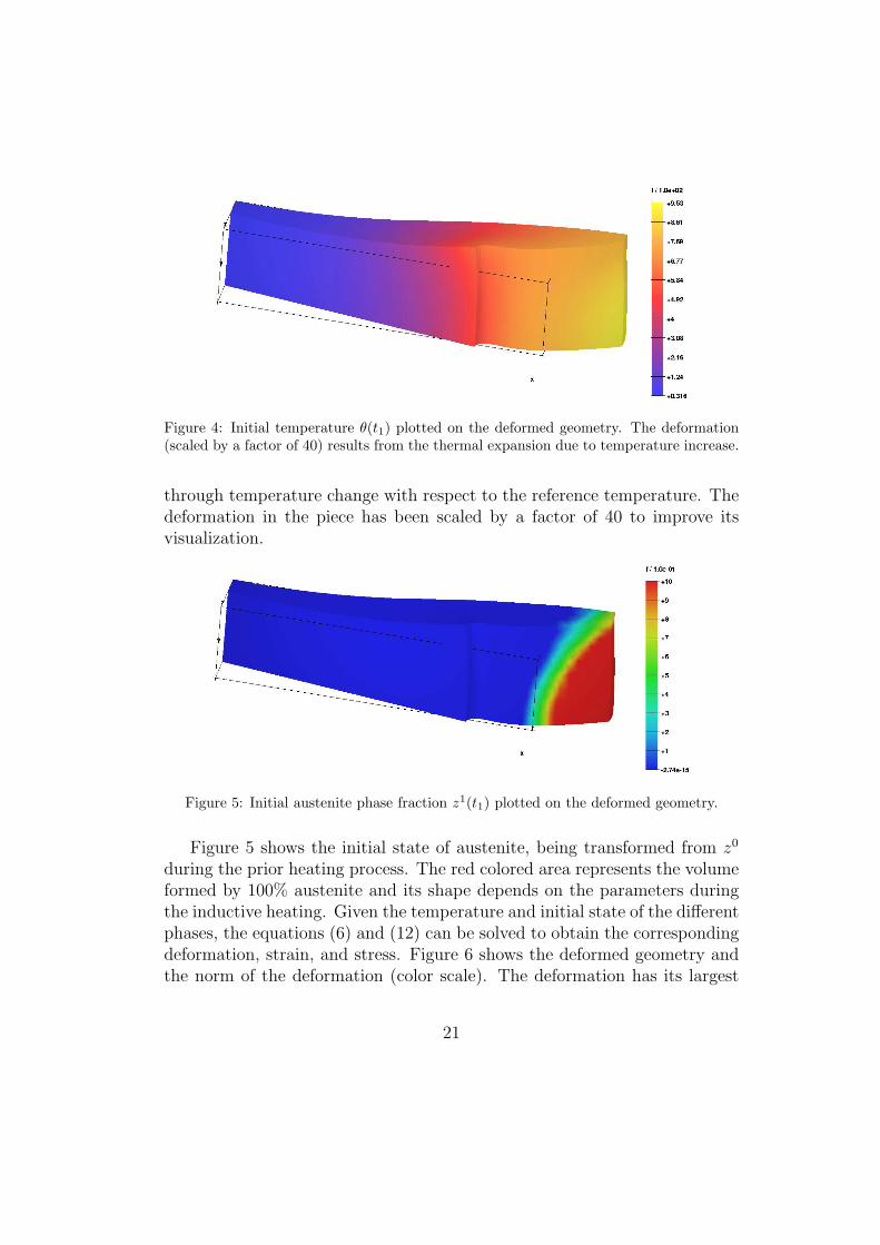
Figure 4: Initial temperature θ(t1) plotted on the deformed geometry. The deformation(scaled by a factor of 40) results from the thermal expansion due to temperature increase.

through temperature change with respect to the reference temperature. Thedeformation in the piece has been scaled by a factor of 40 to improve itsvisualization.

Figure 5: Initial austenite phase fraction z1(t1) plotted on the deformed geometry.

Figure 5 shows the initial state of austenite, being transformed from z0

during the prior heating process. The red colored area represents the volumeformed by 100% austenite and its shape depends on the parameters duringthe inductive heating. Given the temperature and initial state of the differentphases, the equations (6) and (12) can be solved to obtain the correspondingdeformation, strain, and stress. Figure 6 shows the deformed geometry andthe norm of the deformation (color scale). The deformation has its largest

21

Figure 6: Computed norm of the initial deformation ||u(t1)||L2(Ω).

values in the area where the temperature has the largest values as a directeffect of the thermal expansion.

3.5. Numerical results

The simulation based on the material data and initial values from Sections3.3 and 3.4 computes the discrete solutions using the system in equation (56).Table 3 shows the computational expenses to get the results presented below,using the tetrahedral discretization of the geometry as displayed in Figure 3.

Processor: Intel Core i7-2600, 3.4 GHzInstalled RAM: 16.0GBTotal computation time: ca. 26 hMesh nodes: 6514Tetrahedral elements 32246Number of time steps: 11000

Table 3: Computational expenses.

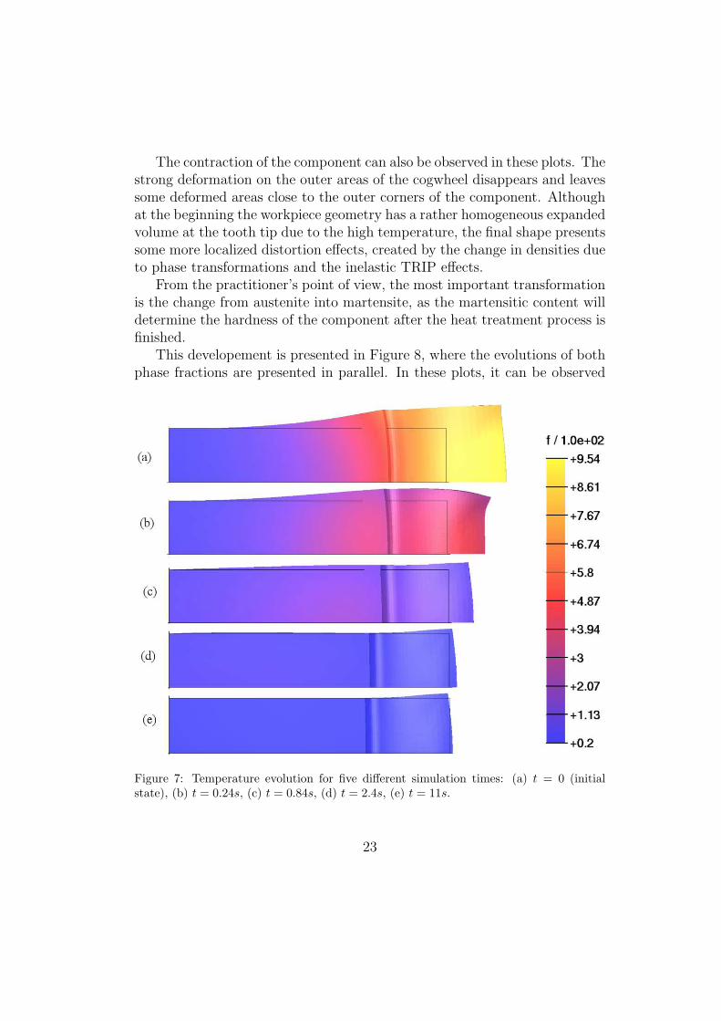
For the quenching simulation, it is clear that the temperature shoulddecrease, producing changes also in the deformation and the phases. Figure7 shows the progressive temperature values on the side view of the deformedgeometries for five different simulated times. In the plots from Figure 7 itcan be observed how the very hot areas cool down in less than one second,getting homogeneous values close to the reference temperature for an elapsedtime of 2.4 seconds.

22

The contraction of the component can also be observed in these plots. Thestrong deformation on the outer areas of the cogwheel disappears and leavessome deformed areas close to the outer corners of the component. Althoughat the beginning the workpiece geometry has a rather homogeneous expandedvolume at the tooth tip due to the high temperature, the final shape presentssome more localized distortion effects, created by the change in densities dueto phase transformations and the inelastic TRIP effects.

From the practitioner’s point of view, the most important transformationis the change from austenite into martensite, as the martensitic content willdetermine the hardness of the component after the heat treatment process isfinished.

This developement is presented in Figure 8, where the evolutions of bothphase fractions are presented in parallel. In these plots, it can be observed

Figure 7: Temperature evolution for five different simulation times: (a) t = 0 (initialstate), (b) t = 0.24s, (c) t = 0.84s, (d) t = 2.4s, (e) t = 11s.

23

how the austenite content gradually disappears, first in the areas close to thecomponent corners (these are also the areas with the fastest heat outflow)and later in the not so close areas. The opposite occurs with the martensiticphase, being inexistent at the beginning and becoming the dominant phase inthe areas close to the corners of the component. Note that all the times shownin Figure 8 correspond to the first second of the quenching process. Afterthis time nothing else is changed, as the minimal activation temperature ofmartensite has already been reached (cf. equation (5)).

The final deformation of the domain corresponds to the typical volumegrowth in areas where the austenite phase is transformed into martensite,changing the density to a lower value (cf. material parameters in Section3.3) and producing the increment in volume.

Much less important is the evolution of ferrite, pearlite and bainite, asthey do not appear in such a fast cooling process. The results in Figure 9 con-firm this, showing the final states for these phase fractions. They are all farfrom reaching any significant amount, so that they can be considered as non

Figure 8: Comparison of austenite and martensite evolutions at different simulation times:(a) t = 0 (initial state), (b) t = 0.24s, (c) t = 0.38s, (d) t = 0.5s, (e) t = 0.98s.

24

existent. Their evolution might become important for different temperatureevolutions and we present them here only for completeness.

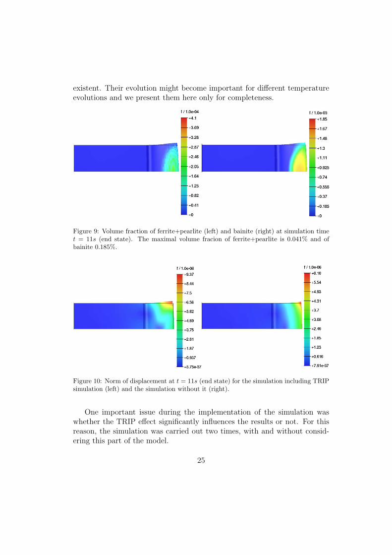
Figure 9: Volume fraction of ferrite+pearlite (left) and bainite (right) at simulation timet = 11s (end state). The maximal volume fracion of ferrite+pearlite is 0.041% and ofbainite 0.185%.

Figure 10: Norm of displacement at t = 11s (end state) for the simulation including TRIPsimulation (left) and the simulation without it (right).

One important issue during the implementation of the simulation waswhether the TRIP effect significantly influences the results or not. For thisreason, the simulation was carried out two times, with and without consid-ering this part of the model.

25

Figure 11: Equivalent (von Mises) stress at t = 11s (end state) for the simulation includingTRIP simulation (left) and the simulation without it (right).

The results of deformation and stress are shown in Figures 10 and 11.It is obvious that both the final deformation and the stress present differentresults in the simulations. Regarding the von Mises stress, the model withTRIP seems to have a smaller area affected by large stresses. The stressdistributions at the end of the simulations are also quantitatively different,giving maximum values of 461 MPa and 816 MPa for the models with andwithout TRIP, respectively. Note that the stress value for the model withoutTRIP can be by far over the yield stress for the 42CrMo4 steel, with valuesaround the 600 MPa.

4. Conclusions

A thermomechanical model for induction surface hardening including oc-curring phase transitions that produce the hardening effect has been inves-tigated. In the simulations of cooling process presented here, owing to highcooling rates most of the austenite is transformed to martensite and the for-mations of ferrit, perlit and bainite are negligible (always less than 0.2%).Concerning the effect of TRIP, a comparison has shown that the consider-ation of TRIP produces significant differences in the results and thereforecannot be neglected.

Although the differences in the models with and without TRIP producedifferent results, it is still not clear if the TRIP is the only inelastic term tobe considered, as also the use of a model for classical plasticity might be of

26

interest.Since only the cooling process has been simulated, the consideration of

efficient solvers for the heating process, i.e. coupled problem of Maxwell’sequation, heat equation and deformation behavior under consideration ofphase transformations is an important direction of further research. An op-tion would be to obtain a heat source from the electromagnetic simulationand then use it for a complete thermomechanical simulation where the heat-ing and quenching processes will be computed together. The simulation ofthe heating process would also allow the consideration of inelastic effects ap-pearing during the temperature increase, either through phase changes orclassical plasticity effects.

Acknowledgements

The authors gratefully acknowledge the financial support of the “Bun-desministerium fur Bildung und Forschung” (BMBF) within the project“Modellierung, Simulation und Optimierung des Mehrfrequenzverfahrens furdie Induktive Warmebehandlung (MeFreSim)” at the University of Bremen.Special thanks go to our cooperation partners within the MeFreSim researchnetwork for providing the material properties and initial data for the simu-lation.

Symbols

θ temperatureθref reference temperatureθext external temperatureiref density of zi(i = 0, . . . , 5) at θref(θ, z) densitycε(θ, z) specific heatk(θ, z) heat conductivityq heat fluxh heat sourceδ(θ, z) heat transfer coefficientu displacementε(u) = 1

2(∇u+∇uT ) strain tensor

εel elastic strainεth thermal strain

27

εtrip TRIP strainσ stress tensorαi(θ) thermal expansion coefficient of phase zi

λ, µ Lame coefficientsK = λ+ 2

3µ bulk modulus

z = (z0, z1, . . . , z5)T vector of phasesLA z0–austenite latent heatLF austenite–ferrite latent heatLP austenite–pearlite latent heatLB austenite–bainite latent heatLM austenite–martensite latent heatFPs ferrite and pearlite start temperatureFPf ferrite and pearlite end temperatureBs bainite start temperatureBf bainite end temperatureMs martensite start temperatureMf martensite end temperature

Kgjl Greenwood-Johnson parameter

References

[1] N. Bontcheva, G. Petzov: Total simulation model of the thermo-mechanical process in shape rolling of steel rods. Comp. Mater. Sci., 34,No. 1, (2009) 377-388.

[2] F.D. Fischer, Q.P. Sun, K. Tanaka: Transformation-Induced Plasticity(TRIP). Appl. Mech. Rev., Vol 49, (1996), p 317-364

[3] F.D. Fischer, G.Reisner, E. Werner, K. Tanaka, G.Cailletaud, T. Antret-ter: A new view on transformation induced plasticity (TRIP). Interna-tional Journal of Plasticity 16 (2000), 723-748.

[4] D. Homberg: A mathematical model for the phase transitions in eutectoidcarbon steel. IMA Journal of Applied Mathematics 54 (1995), 31-57.

[5] D. Homberg: A numerical simulation of the Jominy end-quench test.Acta Mater., 44 (1996), 4375-4385.

[6] D. Homberg: Irreversible phase transitions in steel. Math. Methods Appl.Sci., 20 (1997), 59-77.

28

[7] D. Homberg: A mathematical model for induction hardening includingmechanical effects. Nonlinear Anal. Real World Appl. 5 (2004), 55-90.

[8] J.-B. Leblond, J. Devaux: A new kinetic model for anisothermal metal-lurgical transformations in steels including effect of austenite grain size.Acta Met. 32, (1984), 137-146.

[9] J.-B. Leblond, J. Devaux, J.C. Devaux: Mathematical Modelling of Trans-formation Plasticity in Steels. I: Case of Ideal-Plastic Phases. Int. J. Plast.,Vol 5, (1989), p 551-572

[10] J. Lemaitre, J.-L. Chaboche: Mechanics of Solid Materials. CambridgeUniversity Press, Cambridge, 1990.

[11] T. Miokovic: Analyse des Umwandlungsverhaltens bei ein- undmehrfacher Kurzzeithartung bzw. Laserstrahlhartung des Stahls 42CrMo4.Dissertation, Shaker Verlag Aachen 2005.

[12] J. Montalvo-Urquizo, Z. Akbay, A. Schmidt: Adaptive finite elementmodels applied to the laser welding problem. Comp. Mater. Sci., 46 No. 1,(2009) 245-254.

[13] R. Schroder: Untersuchung zur Spannungs- und Eigenspannungsausbil-dung beim Abschrecken von Stahlzylindern. Dissertation, Universitat Karl-sruhe, 1985.

[14] C. Simsir, C. H. Gr: A FEM based framework for simulation of thermaltreatments: Application to steel quenching. Comp. Mater. Sci. 44 No. 2,(2008) 588-600.

[15] T. Streckenbach, J. Fuhrmann, H. Langmach, M. Uhle: Pdelib–A software toolbox for numerical computations http://www.wias-berlin.de/software/pdelib/ (2010) Retrieved 31.1.2013.

[16] L. Taleb, F. Sidoroff: A Micromechanical Modeling of the Greenwood-Johnson Mechanism in Transformation-Induced Plasticity. Int. J. Plast.,19, (2003), 1821-1842

[17] C. Verdi, A. Visintin: A mathematical model of the austenite-pearlitetransformation in plain steel based on the Scheil’s additivity rule. ActaMetall., 35, No. 11 (1987), 2711-2717.

29

[18] A. Visintin: Mathematical models of solid-solid phase transitions in steel.IMA J. Appl. Math., 39 (1987), 143-157.

[19] M. Wolff, M. Bohm, S. Bottcher: Phase transformations in steel in themulti-phase case - gerneral modelling and parameter identification. Tech-nical Report 07-02, Universitat Bremen, Berichte aus der Technomathe-matik, 2007.

30