Baldwin: Graduate Institute, Geneva, 11a Ave de la Paix, Geneva, Switzerland, baldwin@hei.unige.ch. Harrigan: International Research Department, Federal Reserve Bank of New York, 33 Liberty Street, New York NY 10045, james.harrigan@ny.frb.org. We thank seminar audiences at Columbia, LSE, and the NBER. This paper was written while Harrigan was a Visiting Professor at Columbia University. The views expressed in this paper are those of the authors and do not necessarily reflect the position of the Federal Reserve Bank of New York or the Federal Reserve System.

ZEROS, QUALITY AND SPACE: TRADE THEORY AND TRADE EVIDENCE

Richard Baldwin

Graduate Institute, Geneva, CEPR, and NBER

James Harrigan Federal Reserve Bank of New York, Columbia University, and NBER

June 2007

Abstract Product-level data on bilateral U.S. exports exhibit two strong patterns. First, most potential export flows are not present, and the incidence of these “export zeros” is strongly correlated with distance and importing country size. Second, export unit values are positively related to distance. We show that every well-known multi-good general equilibrium trade model is inconsistent with at least some of these facts. We also offer direct statistical evidence of the importance of trade costs in explaining zeros, using the long-term decline in the relative cost of air shipment to identify a difference-in-differences estimator. To match these facts, we propose a new version of the heterogeneous-firms trade model pioneered by Melitz (2003). In our model, high quality firms are the most competitive, with heterogeneous quality increasing with firms’ heterogeneous cost.

1

1. INTRODUCTION The gravity equation relates bilateral trade volumes to distance and country size. Countless gravity

equations have been estimated, usually with “good” results, and trade theorists have proposed various

theoretical explanations for gravity’s success1. However, the many potential explanations for the

success of the gravity equation make it a problematic tool for discriminating among trade models2.

As a matter of arithmetic, the value of trade depends on the number of goods traded, the amount

of each good that is shipped, and the prices they are sold for. Most studies of trade volumes have not

distinguished among these three factors. In this paper we show that focusing on how the number of

traded goods and their prices differ as a function of trade costs and market size turns out to be very

informative about the ability of trade theory to match trade data.

We establish some new facts about product-level U.S. trade. First, most potential export flows

are not present, and the incidence of these “export zeros” is strongly correlated with distance and

importing country size. Second, export unit values are positively related to distance and negatively

related to market size. We show that every well-known multi-good general equilibrium trade model is

inconsistent with at least some of these facts. We also offer direct statistical evidence of the importance

of fixed costs in explaining export zeros, using the long-term decline in the cost of air shipment to

identify a difference-in-differences estimator.

We conclude the paper with a new version of the heterogeneous-firms trade model pioneered by

Melitz (2003). Our model maintains the core structure of Melitz, which shows how heterogeneity in

firms’ exogenous productivity leads to a market structure where only the most productive firms export.

Unlike Melitz, however, firms in our model differ both in marginal cost and the quality of their goods,

with higher quality goods being both more costly and more profitable. Our model’s predictions are

borne out by the facts established in our data analysis.

Plan of paper

In section 2 we generate testable predictions concerning the spatial pattern of trade flows and

prices. The predictions come from three multi-good general equilibrium models that are representative

1 See Harrigan (2003) for a review. 2 An important exception to this principle is Feenstra, Markusen, and Rose (2001), who show and test how different trade models imply different variations on the gravity model. Our paper is similar in approach, though different in focus.

2

of a wide swath of mainstream trade theory – one based purely on comparative advantage (Eaton and

Kortum 2002), one based purely on monopolistic competition (a multi-country Helpman-Krugman

(1985) model with trade costs), and one based on monopolistic competition with heterogeneous firms

and fixed market-entry costs (a multi-country version of the Melitz (2003) model). These models

predict very different spatial patterns of zeros, i.e. the impact of country size and bilateral distance on

the likelihood of two nations trading a particular product. They also generate divergent predictions on

how observed trade prices should vary with bilateral distance and country size.

Section 3 confronts the theoretical predictions elucidated in Section 2 with highly disaggregated

U.S. data on bilateral trade flows and unit values. On the quantity side, we focus on the pattern of zeros

in product-level, bilateral trade data since this data contains information that is both rich and relatively

unexploited3. Another advantage of focusing on zeros (the extensive margin) rather than volumes of

positive flows (the intensive margin), is that it allows us to avoid issues such as the indeterminacy of

trade flows at the product level in comparative advantage theory and the lack of data on firms’ cost

functions. On the price side, we focus on bilateral, product-specific f.o.b. unit values. When it comes to

empirically confronting the theoretical implications of changes in trade costs, we exploit the fact that

air shipping costs have fallen much faster than the surface shipping costs in recent decades. This opens

the door to a difference-in-difference strategy since our data includes product-level information on air-

versus-surface shipping modes.

All three models fail to explain the broad outlines of the data along at least one dimension. The

best performance is turned in by the heterogeneous-firms trade (HFT) model based on Melitz (2003).

However, this model fails to account for the spatial pattern of trade prices, in particular the fact that

average unit values clearly increase with distance while the HFT model predicts that they should

decrease with distance. Section 4 therefore presents a new model in which firms compete on the basis

of heterogeneous quality as well as unit costs, with high quality being associated with high prices.

Since a nation’s high-quality/high-price goods are the most competitive, they more easily overcome

distance-related trade costs so the average price of goods in distant markets tends to be higher.

3 We are not the first to exploit zeros. Haveman and Hummels (2004) is similar in sprit to our paper, although they focuses on import zeros. Feenstra and Rose (2000) and Besedes and Prusa (2006a, 2006b) have looked at time-series variation in product level zeros to test trade models.

3

2. ZEROS AND PRICES IN THEORY This section derives testable hypotheses concerning the spatial pattern of zeros and trade prices in

models that represent a broad swath of trade theory. In the three models selected, trade is driven by: 1)

comparative advantage, 2) monopolistic competition, and 3) monopolistic competition with

heterogeneous firms.

The models we study share some assumptions and notation. There are C countries and a

continuum of goods. Preferences are given by the indirect CES function,

( )1

1 1, , 1ii

EU P p diP

σ σ σ− −

∈Θ= ≡ >∫ . (1)

where E is nominal expenditure, pi is the price of variety i, and Θ is a set of available varieties.

Transport costs are assumed to be of the iceberg form, with τod ≥ 1 representing the amount of a good

which must be shipped from nation-o to nation-d for one unit to arrive (o stands for “origin”, and d

stands for “destination”). All the models assume just one factor of production in fixed supply, labor,

which is paid a wage w.

2.1. Comparative advantage: Eaton-Kortum

Economists have been thinking about the effects of trade costs on trade in homogeneous goods since

Ricardo, but we had to wait for Eaton and Kortum (2002) to get a clear, rigorous, and flexible account

of how distance affects bilateral trade in a competitive general equilibrium trade model. Appendix 1

presents and solves a slightly simplified Eaton-Kortum model (EK for short) explicitly. Here we

provide intuition for the EK model’s predictions on the spatial pattern of zeros and prices.

Countries in the EK model compete head-to-head in every market on the basis of c.i.f. prices,

with the low-price supplier capturing the whole market4. This “winner takes all” form of competition

means that the importing country buys each good from only one source. As usual in Ricardian models,

the competitiveness of a country’s goods in a particular market depends upon the exporting country’s

technology, wage and bilateral trade costs – all relative to those of its competitors. A key novelty of the

EK model is the way it describes each nation’s technology. The EK model does not explicitly specify

each nation’s vector of unit-labor input coefficients (the a’s in Ricardian notation). Rather it views the 4 c.i.f. and f.o.b. stand for “cost, insurance, and freight” and “free on board”, respectively, i.e. the price with and without transport costs. Without domestic sales taxes, c.i.f. and f.o.b. correspond to the consumer and producer prices respectively.

4

national vectors of a’s as the result of a stochastic technology-generation process – much like the one

used later by Melitz (2003). Denoting the producing nation as nation-o (‘o’ for origin), and the unit

labor coefficient for a typical good-j as ao(j), each ao(j) is an independent draw from the cumulative

distribution function (cdf)5

0[ ] 1 , , 0, 1, 1,...,oT aoF a e a T o N

θ

θ−= − ≥ > = (2)

where To > 0 is the nation-specific parameter that reflects the nation’s absolute advantage, and N is the

number of nations.

Equation (2) makes it possible to calculate the probability that a particular nation has a

comparative advantage in a particular market in a typical good. Since the ao(j)’s for all nations are

random variables, determining comparative advantage becomes a problem in applied statistics. Perfect

competition implies that nation-o will offer good-j in destination nation-d at a price of

)()( jawjp ooodod τ= where wo is nation-o’s wage. As the appendix shows, this implies that the

distribution of prices in typical market-d in equilibrium is

1

[ ] 1 exp ; ,( )

N cd d d id cdc

c cd

TG p p T Tw

θθτ=

⎡ ⎤= − −∆ ∆ ≡ ≡⎣ ⎦ ∑ (3)

Given (3) and (2), the probability that origin nation-o has comparative advantage in destination nation-

d for any product is6

odod

d

Tπ =∆

(4)

This probability, which is the key to characterizing the spatial pattern of zeros in the EK model, reflects

the relative competitiveness of nation-o’s goods in market-d. Namely, Tod is inversely related to o’s

average unit-labor cost for goods delivered to market-d, so πod is something like the ratio of o’s average

unit-labor cost to that of all its competitors in market-d.7

5 EK work with z=1/a, so their cdf is exp(-T/zθ). 6 Technology draws are independent across goods, so this is valid for all goods. See the appendix for details. 7 Nation-o’s unit-labour cost, averaged over all goods with (2), for goods delivered to d is τodw/T1/θ ; this equals 1/(Tod)θ.

5

The EK model does not yield closed-form solutions for equilibrium wages, so a closed form

solution for πod is unavailable. We can, however, link the Tod’s to observable variables by employing

the market clearing conditions for all nations (see appendix for details). In particular, wages must

adjust to the point where every nation can sell all its output and this implies

1( / )

dod o

od d d c d c c oc

PYY P Y P

θ

θ θπτ τ≠

⎛ ⎞ ⎛ ⎞= ⎜ ⎟ ⎜ ⎟+ Σ⎝ ⎠ ⎝ ⎠

(5)

where the Y’s are nations’ total nominal output (GDP), the P’s are nations’ price indices from (1), and

the set of the continuum of goods [ ]0,1Θ = . While this is not a closed form solution, the export

probability is expressed in terms of endogenous variables for which we have data or proxies.

2.1.1. Predicted spatial pattern of zeros and trade prices in the Eaton-Kortum model

Equation (5) gives the sensible prediction that the probability of o successfully competing in

market-d is decreasing in bilateral transport costs. The incidence of export zeros (that is, products

exported to at least one but not all potential markets) should be increasing in distance if distance is

correlated with trade costs, and import zeros (products imported from at least one potential source but

not all) should predominate since each importer buys each good from just one supplier.

For tractability, the EK model assumes that iceberg trade costs are the same for all goods that

travel from o to d. Harrigan (2006) shows that allowing for heterogeneity in trade costs across goods in

a simplified version of EK introduces a further role for relative trade costs to influence comparative

advantage. For our purposes here, the main interest of Harrigan (2006) is the result that a fall in

variable trade costs for a subset of goods leads to an increase in the probability that they will be

successfully exported.

The role of market size in determining the probability of exporting can also be studied with (5).

The bigger is market-d, as measured by its GDP Yd, the smaller is the probability that o successfully

sells in d. There are two elements to the intuition of this result. Large countries must sell a lot so they

need, on average, low unit-labor-costs (as measured by woθ/To) and this means that large nations are

often their own low-cost supplier. The second is that there are no fixed market-entry (i.e. beachhead)

costs, so that an exporter will supply all markets where it has the lowest c.i.f. price regardless of how

tiny those markets might be. Expression (5) also predicts that nation-d imports more goods from larger

exporters, with size measured by Yo.

6

The EK model makes extremely simple predictions for the spatial distribution of import prices.

The distribution of prices inside nation-d is given by (3) and each exporting nation has a constant

probability of being the supplier of any given good. Consequently, the c.i.f. price of nation-o’s exports

to nation-d is just a random sample from (3), which means (3) also describes the distribution of import

prices for every exporting nation. The average c.i.f. price of goods imported from every partner should

be identical and related to nation-d price index by (see appendix for details)

⎟⎟⎠

⎞⎜⎜⎝

⎛+Γ+−Γ

=]/)1[(

]/)1[(θθθθσ

deod Pp (6)

where Γ[.] is the Gamma function. Since trade costs are fully passed on under perfection competition,

the average bilateral export (f.o.b.) price, odeodp τ/ , should be increasing in the destination nation’s

price index and declining in bilateral distance.

2.1.2. Extensions and modifications of the Eaton-Kortum model

The EK model is a multi-country Ricardian model with trade costs. In all Ricardian models, the

locus of competition is within each destination nation. This means that exporters must meet the

competitive demands in each nation if they are to export successfully. Given this basic structure, the

prediction of equal average import prices from all source nations is quite robust. Putting it differently,

highly competitive nations export a wider range of goods than less competitive nations but the average

import price of their goods does not vary with exporter’s competitiveness, size or distance from the

importing market. Staying in the Ricardian-Walrasian framework limits the range of modifications and

extensions, so most extensions and modifications of the EK model lead to quite similar spatial

predictions for zeros and prices.

One important extension of EK is Bernard, Eaton, Jensen and Kortum (2003). This model

introduces imperfect competition into the EK framework with the low-cost firm in each market

engaging in limit pricing. Limit pricing ties the market price to the marginal cost of the second-best

firm, rather than the first-best as in EK. However with randomly generated technology, the outcome for

the spatial pattern of zeros and prices is qualitatively unaltered.

Eaton, Kortum and Kramarz (2005) modify the EK framework model further, and the resulting

model is completely out of the Walrasian framework. The paper introduces monopolistic competition

(thus deviating from perfect competition) and fixed market-entry, i.e. beachhead costs (thus deviating

7

from constant returns). Eaton, Kortum and Kramarz (2005) is thus best thought of as an HFT model,

which we consider in Section 2.3.

2.1.3. Summary of empirical implications of the Eaton-Kortum model

We conclude this section with a recap of what the EK model predicts about zeros and prices across

space.

Export zeros The probability that exporter-o sends a good to destination-d is decreasing in the

distance between o and d, and also decreasing in the size of d. A fall in trade

costs reduces the incidence of zeros.

Export prices Considering a single product sold by o in multiple destinations d, the f.o.b price

is decreasing in the distance between o and d, and unrelated to the size of d.

2.2. Monopolistic competition

Monopolistic competition (MC) models constitute another major strand in trade theory. The particular

MC model that we focus on, like the Eaton-Kortum model, has N countries, iceberg trade costs and a

single factor of production L. The trade structure, however, is starkly different. Because of the love-of-

variety in demand, every good is consumed in every country and the same f.o.b. prices are charged to

every market. Goods are produced under conditions of increasing returns and Dixit-Stiglitz

monopolistic competition. Firms are homogenous in that they all face the same unit-labor requirement,

a. The model is very standard, so we will move quickly (see Appendix for details).

Dixit-Stiglitz competition implies that ‘mill pricing’ is optimal, i.e. firms charge the same f.o.b.

export price regardless of destination, passing the iceberg trade cost fully on to consumers. With mill

pricing and CES demand, the value of bilateral exports for each good is

11

1; [0,1], .1 1/

o d dod od d od od d

d

w a w Lv B BP

σσ

σφ φ τσ

−−

−

⎛ ⎞= ≡ ∈ ≡⎜ ⎟−⎝ ⎠ (7)

where vod is the value of bilateral exports for a typical good, φod reflects the ‘freeness’ of bilateral trade

(φ ranges from zero when τ is prohibitive to unity under costless trade, i.e. τ = 1), Bd is the per-firm

demand-shifter in market-d, and Pd is as in (5), with Θ being the set of goods sold in d.

8

2.2.1. Spatial pattern of zeros and prices in the monopolistic competition model

Consumers in the MC model buy some of every variety with a finite price, so there should be

no zeros in exporters’ bilateral trade matrices: if a good is exported to one country it is exported to all.

The size of the export market has no bearing on this prediction, since in the absence of fixed market

entry costs firms find it profitable to sell even in tiny markets.

The MC model also has sharp predictions for the spatial pattern of trade prices. Mill pricing is

optimal, so the f.o.b. export price for all destinations should be identical. Since trade costs are passed

fully on to consumers, the c.i.f. import prices should increase with bilateral distance but there should be

no connection between market size and pricing (f.o.b. or c.i.f).

2.2.2. Extensions and modifications of the monopolistic competition model

The core elements of the MC model are imperfect competition, increasing returns and

homogenous firms. Since imperfect competition can take many forms, many variants of the standard

MC model are possible. The general formula for optimal pricing under monopolistic competition sets

consumer price to 11od

d

aτε −−

, where εd is the perceived elasticity of demand in market-d. Different

frameworks link εd to various parameters. Under Dixit-Stiglitz monopolistic competition, εd equals σ.

Under the Ottaviano, Tabuchi and Thisse (2002) monopolistic competition framework firms face linear

demand, so εd rises as firms move up the demand curve. This means that the markup falls as greater

trade cost drive consumption down. In other words, producers absorb some of the trade costs, so the

f.o.b. export prices should be lower for more distant markets. Linear demand also implies that there is a

choke-price for consumers and thus trade partners that have sufficiently high bilateral trade costs will

export nothing to each other. A corollary is that a fall in trade costs will reduced the incidence of zeros.

Finally, if demand curves are sufficiently convex, higher bilateral trade costs raise the markup and this

implies that f.o.b. prices can rise with distance. Because this degree of convexity implies a

counterfactual more-than-full pass-through of cost shocks (e.g., more than 100% exchange rate pass-

through) such demand structures are not typically viewed as part of the standard MC model.

Likewise, many forms of increasing returns are possible. The no-zeros prediction of the

standard MC model stems from the fact that consumers buy some of every good provided only that

prices are finite. If in additional to iceberg trade costs, one assumes that there are beachhead costs (i.e.

fixed market entry costs), then nation-o sell its varieties to nation-d only if bilateral trade is sufficiently

9

free. With the Ottaviano et. al. framework, the predicted pattern of zeros is very stark. Nation-o’s

export matrix has either no zero with respect to nation-d, or all zeros.

2.2.3. Summary of empirical implications of monopolistic competition model

We conclude this section with a recap of what the monopolistic competition model predicts about zeros

and prices across space. We consider both the baseline model with CES preferences as well as the

Ottaviano et. al. model with linear demand.

Export zeros The baseline model predicts zero zeros: if an exporter-o sends a good to any

destination-d it will send the good to all destinations. With linear demand, the

probability of a zero is increasing in the distance between o and d, but unrelated

to the size of d. A fall in trade costs will reduce the probability of zeros with

linear demand.

Export prices Considering a single product sold by o in multiple destinations, the baseline

model predicts no variation in f.o.b export prices. With linear demand, the f.o.b

price is decreasing in the distance between o and d, and unrelated to the size of d.

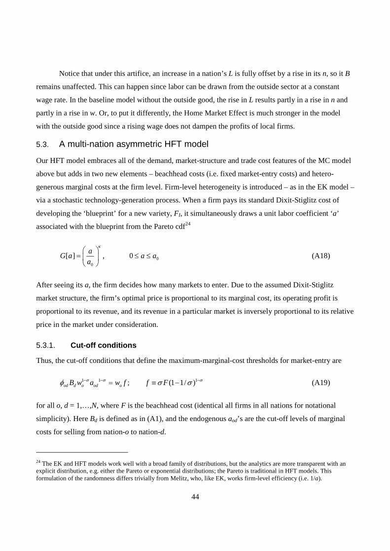
2.3. A multi-nation asymmetric heterogeneous firms trade model

One of the beauties of the original Melitz (2003) heterogeneous firms trade (HFT) model is that it

provides a clean and convincing story about why some products are not exported at all. But since

Melitz (2003) works with two or more symmetric countries, it can not address the spatial pattern of

export zeros or export prices. Here we develop a multi-country HFT model with asymmetric countries

and arbitrary trade costs to generate testable hypotheses concerning zeros and prices.

The HFT model we work with embraces all of the features of the baseline monopolistic

competition model and adds in two new elements – fixed market-entry (beachhead) costs and

heterogeneous marginal costs at the firm level. Firm-level heterogeneity is introduced – as in the Eaton-

Kortum model – via a stochastic technology-generation process. When a firm pays its set-up cost FI it

simultaneously draws a unit labor coefficient from the Pareto distribution,8

8The HFT model is easily solved with an exponential cdf like (2), but (8) is more traditional and can be justified by reference to data on the U.S. firm size distribution (Axtell, 2001). This formulation of randomness differs trivially from Melitz, who, like EK, works firm-level efficiency (i.e. 1/a).

10

00

[ ] ; 1, 0aG a a aa

κ

κ⎛ ⎞

= > ≤ ≤⎜ ⎟⎝ ⎠

(8)

After seeing its’ a, the firm decides how many markets to enter. As in the MC model, Dixit-Stiglitz

competition means that a firm’s optimal price is proportional to its marginal cost, its operating profit is

proportional to its revenue, and its revenue is inversely proportional to its relative price. Thus a firm

that draws a relatively high marginal cost earns little if it does produce. If this amount is insufficient to

cover the beachhead cost in any market, the firm never produces. Firms that draw lower marginal costs

may find it profitable to enter some markets (especially their local market where the absence of trade

costs provides them with a relative cost advantage). More generally, each export market has a threshold

marginal cost for every origin nation, i.e. a maximum marginal cost that yields operating profit

sufficient to cover the beachhead cost. Using (7), the cut-off conditions that define the bilateral

maximum-marginal-cost thresholds aod are9

1 1; (1 1/ )od d o odB w a f f Fσ σφ σ σ− −= ≡ −

so

111 d

o odod

Bw af

σ

τ

−⎛ ⎞= ⎜ ⎟

⎝ ⎠ (9)

for all nations.

In Melitz’ original model with symmetric countries, the additional assumption of the Pareto

distribution for marginal cost makes it possible to obtain analytical solutions for all the endogenous

variables, including wages and per-firm demands (Baldwin (2005)). With asymmetric countries

solution is more difficult. The approach taken by Helpman, Melitz, and Yeaple (2004) is to assume the

existence of a costlessly traded constant returns numeraire sector10. If all countries produce the

numeraire good in equilibrium (which parameter restrictions can guarantee), then wages are equalized

across countries and the per-firm demand levels Bd are independent of market size (see appendix). This

9 Here we have chosen units (without loss of generality) such that a0=1. We also assume the regularity condition κ > σ -1, and that beachead costs are the same everywhere for notational simplicity. 10 This solution approach has also been taken by Demidova (2006) and Falvey, Greenaway, and Yu (2006) in their analyses of a two-country asymmetric HFT model.

11

has the counterfactual implication that, controlling for distance, a given exporting firm has the same

level of sales in every market. The economics behind this result is that larger markets attract greater

numbers of entrants, which reduces demand levels facing every firm below what they would be in the

absence of entry. In equilibrium, entry exactly offsets country size differences, so that demand levels

for a given firm are the same regardless of which market they sell in.

An alternative solution procedure is to dispense with the assumption of a costlessly traded

equilibrium and to analyze Melitz’ original model with the single change of allowing for differences in

country size. As we show in the appendix, it is not possible to solve this model analytically, but

numerical simulation is straightforward. We show that larger countries have larger per-firm demands,

and as a result any given firm sells more to larger countries than to smaller ones (controlling for trade

costs). The mechanism is that larger countries have endogenously higher nominal wages, which leads

to less entry than there would be if wages were equalized. A way to see the contrast between the two

solutions is to note that incipient entry raises the demand for labor in the larger country, but that this

has different effects depending on the behavior of wages. When wages are fixed by the numeraire

sector, all the adjustment takes place through entry. Without the numeraire sector, part of the

adjustment comes through higher nominal wages in the larger country, which dampens entry and

consequently leaves per-firm demand higher in the larger country.

2.3.1. Asymmetric HFT’s spatial pattern of zeros and prices

The spatial pattern of zeros comes from the cut-off thresholds. The probability that a firm producing

variety-j with marginal costs woao(j) will exports to nation-d is the probability that its marginal cost is

less than the threshold defined in (9), namely

1/

1Pr ( ) d do o

od od

B Bw a jf f

κ

β κ βτ τ

⎧ ⎫⎛ ⎞⎪ ⎪< =⎨ ⎬⎜ ⎟⎝ ⎠⎪ ⎪⎩ ⎭

(10)

where we used (8) to evaluate the likelihood. In our empirics, we only have data on products that are

actually exported to at least one market so it is useful to derive the expression for the conditional

probability, i.e. the probability that firm h exports to market j given that it exports to at least one

market. This conditional probability of exports from o to d by typical firm j is

12

min

od d

i o oi i

BB

κ

κ

ττ

−

−≠

(11)

Since we work with data for a single exporting nation, the denominator here will be a constant for all

products. Thus the probability that an exporting firm exports to a given market is predicted to decline

as the distance to that market increases, and increase as the market size rises. A fall in variable trade

costs increases the marginal cost cutoff for profitable exporting, and hence reduces the probability of

export zeros.

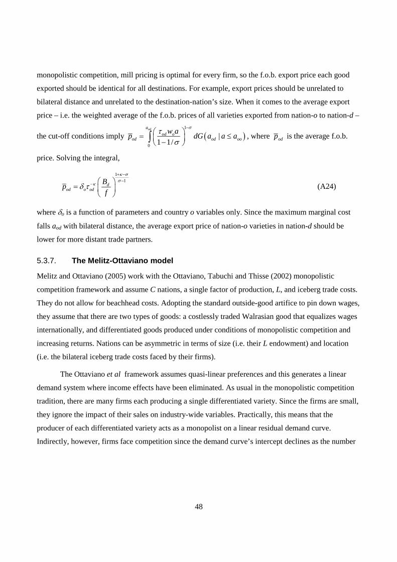
The spatial pattern of prices in the asymmetric HFT model is also simple to derive. We consider

both the export (f.o.b.) price for a particular good exported to several markets, and the average export

(f.o.b.) price for all varieties exported by a particular nation. Because the model relies on Dixit-Stiglitz

monopolistic competition, mill pricing is optimal for every firm, so the f.o.b. export price of each good

exported should be identical for all destinations. In particular, the export price for any given good

should be unrelated to bilateral distance and unrelated to the size of the exporting and importing

nations. However, the range of goods exported does depend on bilateral distance and size, so the

average bilateral f.o.b. export price will differ systematically. The cut-off conditions (9) imply that the

weighted average of the f.o.b. prices of all varieties exported from nation-o to nation-d, odp , is

( )1

0

|1 1/

odaod o

od od oow ap dG a a a

στσ

−⎛ ⎞= ≤⎜ ⎟−⎝ ⎠∫

Using (8) to evaluate the integral and eliminating the cutoff aod using (9), this becomes

11

o dod

od

Bpf

κ σσ

κ

δτ

+ −−⎛ ⎞

= ⎜ ⎟⎝ ⎠

(12)

where δo is a function of parameters and country o variables only. Equation (12) implies that the

relative average export price to any two markets c and d from a single origin o depends only on relative

distance from o and relative market size:

11

od oc d

oc od c

p Bp B

κ σκστ

τ

+ −−⎛ ⎞ ⎛ ⎞

= ⎜ ⎟ ⎜ ⎟⎝ ⎠ ⎝ ⎠

13

The logic of (12) is that since the cut-off marginal cost, aod, falls with bilateral distance and increases

with market size, the average export price of nation-o varieties to nation-d should be decreasing in

distance and increasing in the size of the export market. The intuition is that the cheapest goods are the

most competitive in this model, so they travel the furthest.

2.3.2. Extensions and modifications of the asymmetric HFT model

The asymmetric HFT model, like the monopolistic competition model, has imperfect

competition and increasing returns as core elements. As noted above, there are many different forms of

imperfect competition and scale economies. The other core elements of the HFT model are beachhead

costs or choke-prices (these explain why not all varieties are sold in all markets) and heterogeneous

marginal costs (these explain why some nation-o firms can sell in a market but others cannot). This

suggests three dimensions along which HFT models can vary: market structure, source of scale

economies, and source of heterogeneity.

For example, Eaton, Kortum, and Kramarz (2005) present a model that incorporates beachhead

and iceberg costs in a setting that nests the Ricardian framework of Eaton-Kortum (2002) and Bernard

et al (2003) with the monopolistic competition approach of Melitz (2003). Eaton et. al. does not include

set-up costs since firms’ are endowed with a technology draw. Another difference is that they work

with a technology-generating function from the exponential family. Demidova (2005) and Falvey,

Greenaway and Yu (2006) allow for technological asymmetry among nations but embrace Dixit-

Stiglitz competition with icebergs, beachhead and set-up costs. Yeaple (2005) assumes the source of

the heterogeneous marginal costs stems from workers who are endowed with heterogeneous

productivity; he works with Dixit-Stiglitz monopolistic competition with icebergs and beachhead costs.

As these models all involve Dixit-Stiglitz monopolistic competition, icebergs and beachhead costs,

their spatial predictions for zeros and price are qualitatively in line with the model laid out above.

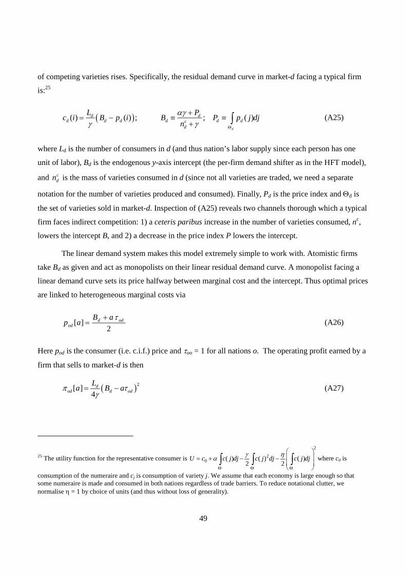
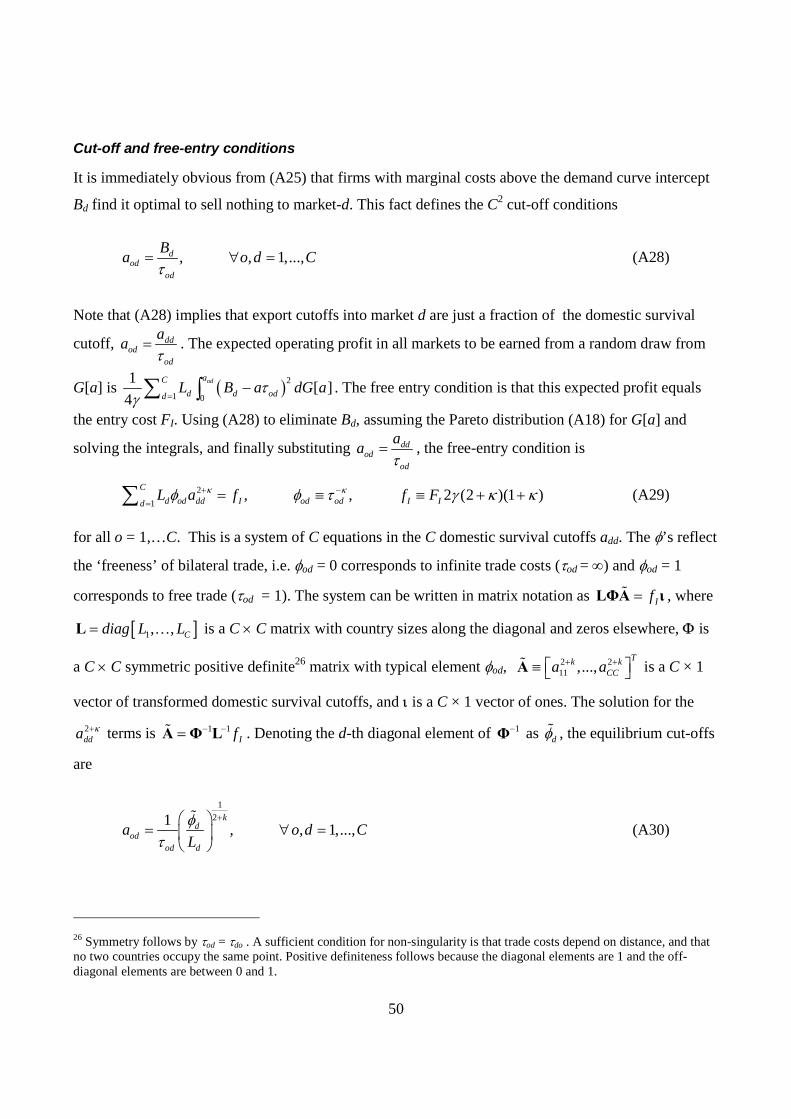
Melitz and Ottaviano (2005) work with the Ottaviano, Tabuchi, and Thisse (2002) monopolistic

competition framework with linear demands. The implied choke-price substitutes for beachhead costs

in shutting off the trade of high-cost varieties. The Melitz-Ottaviano prediction for the spatial pattern of

zeros matches that of the asymmetric HFT model with respect to bilateral distance, but not with respect

to market size. As our appendix illustrates, the cut-off marginal cost in Melitz-Ottaviano is tied to the

y-axis intercept of the linear residual demand curve facing a typical firm. More intense competition

14

lowers this intercept (this is how pure profits are eliminated in the model) and thus the cut-off (aod in

our notation) falls with the degree of competition. Since large nations always have more intense

competition from local varieties, Melitz-Ottaviano predicts that large countries should have lower cut-

offs, controlling for the nation’s remoteness. In other words, Melitz-Ottaviano predicts a positive

relationship between the size of the partner nation and the number of zeros in an exporter’s matrix of

bilateral, product-level exports. As far as the spatial pattern of prices is concerned, Melitz-Ottaviano

predict that export prices should decline with the market’s distance and with market size, a result which

follows from the result that the cutoffs are declining in distance and market size.

2.3.3. Summary of empirical implications of asymmetric HFT model

We conclude this section with a recap of what the asymmetric HFT model predicts about zeros and

prices across space. We consider both the baseline model with CES preferences as well as the Melitz-

Ottaviano et. al. model with linear demand.

Export zeros The probability of an export zero is increasing in bilateral distance. The effect of

market size on the probability of an export zero is negative in the baseline

model, and positive in the Melitz-Ottaviano variant. A decline in trade costs

reduces the incidence of zeros.

Export prices Considering a single product sold by o in multiple destinations, the f.o.b price is

decreasing in the distance between o and d. The effect of market size on average

f.o.b. price is positive in the baseline model, and negative in the Melitz-

Ottaviano variant.

3. ZEROS AND PRICES IN TRADE DATA The models described in the previous section all make predictions about detailed trade data in a

many country world. These predictions are collected for easy reference in the first five rows of Table 1.

To evaluate these predictions, we use the most detailed possible data on imports and exports – the trade

data collected by the U.S. Customs Service and made available on CD-ROM.

For both U.S. imports and U.S. exports, the Census reports data for all trading partners

classified by the 10-digit Harmonized System (HS). For each country-HS10 record, Census reports

value, quantity, and shipping mode. In addition, the import data include shipping costs and tariff

15

charges. Our data analysis also includes information on distance and various macro variables, which

come from the Penn-World Tables.

The Census data are censored from below, which means that very small trade flows are not

reported. For imports, the cut-off is $250, so the smallest value of trade reported is $251. For exports,

the cut-off is 10 times higher, at $2500. This relatively high censoring level for exports is a potential

problem, since there may be many economically meaningful export relationships which are

inappropriately coded as nonexistent. One hint that this problem is not too prevalent comes from the

import data, where only 0.8% of the non-zero trade flows are between $250 and $2500.

3.1. How many zeros?

We define a zero as a trade flow which could have occurred but did not. For exports, a zero

occurs when the U.S. exports an HS10 product to at least one country but not all. The interpretation of

an export zero is simple, since they are defined only for goods actually produced. For imports, a zero is

an HS10 good which is imported from at least one country but not all. The interpretation of an import

zero is not as simple; they may be defined in cases when the country in question does not even produce

the good (the U.S. has zero imports of bananas from Canada, for example).

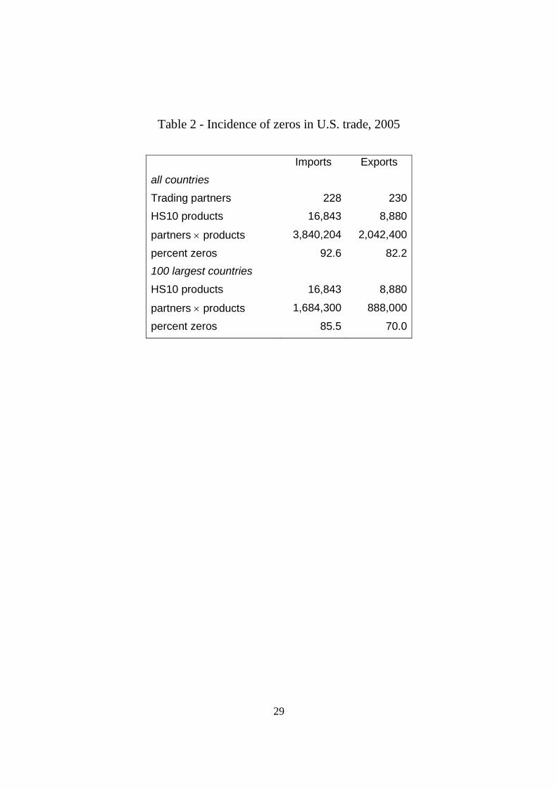
The incidence of zeros in U.S. trade in 2005 is reported in Table 2. The United States imported

in nearly 17,000 different 10-digit HTS categories from 228 countries, for a total of over 3.8 million

potential trade flows. Over 90% of these potential trade flows are zeros. The median number of

supplier countries was 12, with a quarter of goods being supplied by at least 23 countries. Only 5% of

goods have a unique supplier. In principle this pattern of imports is consistent with a homogeneous

goods model, since if we define a good narrowly enough it will have just one supplier (“red wine from

France”). However, the large number of suppliers for the majority of narrowly defined goods seems

instead to be suggestive of product differentiation11. This well-known phenomenon is part of what

motivated the development of monopolistic competition trade models.

Zeros are almost as common in the export data as in the import data. Table 2 shows that in 2005

the U.S. exported 8,880 10-digit goods to 230 different destinations, for a total of more than 2 million

potential trade flows. Of these, 82% are zeros. Unlike the import zeros these have an unambiguous

interpretation, since a zero is defined only if a good is exported to at least one country, which 11 The largest number of trading partners for any product is 125, for product 6204.52.2020, “Women’s trousers and breeches, of cotton, not knitted or crocheted”. This is not a homogeneous goods category.

16

necessarily means the good is produced in the U.S. The median number of export markets is 35, with a

quarter of goods exported to at least 59 markets. Only 1% of products are sent to a unique partner.

Many of the 230 places that the U.S. trades with are tiny to the point of insignificance (Andorra,

Falkland Islands, Nauru, Pitcairn, Vatican City, and the like). Restricting attention to the 100 large

countries for which we have at least some macroeconomic data reduces the incidence of zeros

somewhat (86% for imports, 70% for exports), but does not fundamentally change the message that

zeros predominate.

The predominance of export zeros is at odds with the “zero zeros” prediction of the baseline

monopolistic competition model with CES preferences discussed in Section 2. Thus even before we

proceed to formal statistical analysis we conclude that this model is a non-starter.

3.2. Export zeros across space

The gravity equation offers a flexible and ubiquitous statistical explanation for the aggregate

volume of trade between countries. The basic logic of the gravity equation is simplicity itself: bilateral

trade volumes depend positively on country size and negatively on distance. Here we adopt the gravity

approach to explain not the volume of trade but rather its incidence. This descriptive statistical exercise

is intended to help us understand the pattern of export zeros summarized in Table 2.

We focus on U.S. export zeros because of their unambiguous interpretation as products which

the U.S. produces and ships to at least one, but not all, countries. Extending the gravity logic suggests

that exports should be more likely the larger the production of the good, the larger the export market,

and the shorter the distance the good would have to travel. We have no information on production

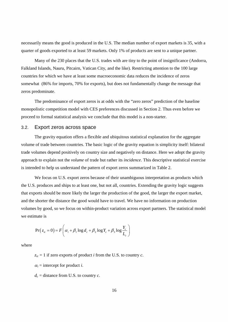
volumes by good, so we focus on within-product variation across export partners. The statistical model

we estimate is

( ) 1 2 3Pr 0 log log log cic i c c

c

Yz F d YL

α β β β⎛ ⎞

= = + + +⎜ ⎟⎝ ⎠

where

zic = 1 if zero exports of product i from the U.S. to country c.

αi = intercept for product i.

dc = distance from U.S. to country c.

17

Yc = real GDP of country c.

Lc = labor force in country c.

and F is a probability distribution function. There is no particular reason to expect the relationship to be

linear, so we allow the relationship between zeros and distance to be a step function and also include

GDP per worker (aggregate productivity) as a control. The distance step function is specified by

looking for natural dividing points in the raw distance data, and the countries in each category are listed

in Table 3. As indicated in Table 2, the dimensions of the data in 2005 are 8,880 HS10 products and

100 countries. As is well known, fixed effects logit and probit estimators are not consistent when the

number of effects is large. As a consequence, we estimate two other statistical models, the linear

probability and random effects logit models, with results reported in Table 3.

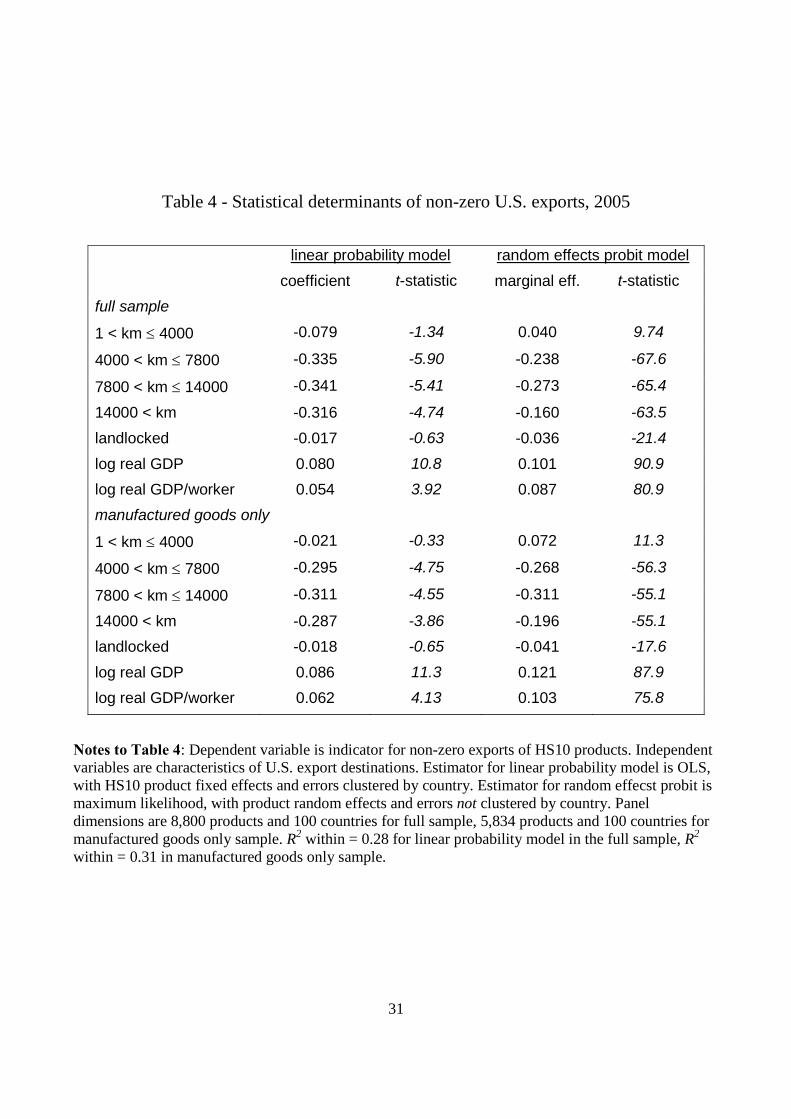
The first two columns of Table 4 report the results of the linear probability model. The

coefficients have the simple interpretation as marginal effects on the probability of a good being

exported to a particular country, conditional on being exported to at least one country. The excluded

distance category of 0 kilometers includes the United States and Canada. For nearby countries distance

has no statistically significant effect on zeros, an effect which jumps to about 0.33 for distances greater

than 4000km. Country size also has a very large effect, with a 10% increase in real GDP of the

importing country lowering the probability of a zero by 8 percentage points. The importer’s aggregate

productivity also has a large effect, with a 10% increase raising the probability of trade by more than 5

percentage points. Except for the aggregate productivity effect the sign of the estimated effects is not

surprising, but it is useful to see how large the magnitudes are.12 The within R2 of 0.28 is quite high by

the standards of cross-section regressions. The results are very similar for the sample restricted to HS

codes that belong to SITC 6 (manufactured goods), 7 (machinery and transport equipment), and 8

(miscellaneous manufactures).

The final two columns of Table 4 report marginal effects from the random effects logit. There

are two strong technical assumptions behind these computations which give reasons to be skeptical of

the results: first, the assumption that the random product effects are orthogonal to country

characteristics is a strong one which can be rejected statistically, and second, the covariance matrix

estimator doesn’t permit clustering errors by country (which amounts to assuming that errors for each

12 The large effect of aggregate productivity may be related to the mechanism recently studied by Choi, Hummels and Xiang (2006).

18

export market are independent across goods). In any event, the marginal effects from the logit are

broadly consistent with the coefficients of the linear probability model, which suggests that the

functional form assumption of the former model doesn’t do too much violence to the data. As with the

linear probability model, splitting the sample does not change much.

While in many respects not surprising, the results of Table 4 are not consistent with most of the

models summarized in Table 1. Only the heterogeneous firm model with CES preferences is consistent

with the positive market size and negative distance effects identified in the data.

3.3. Export unit values across space

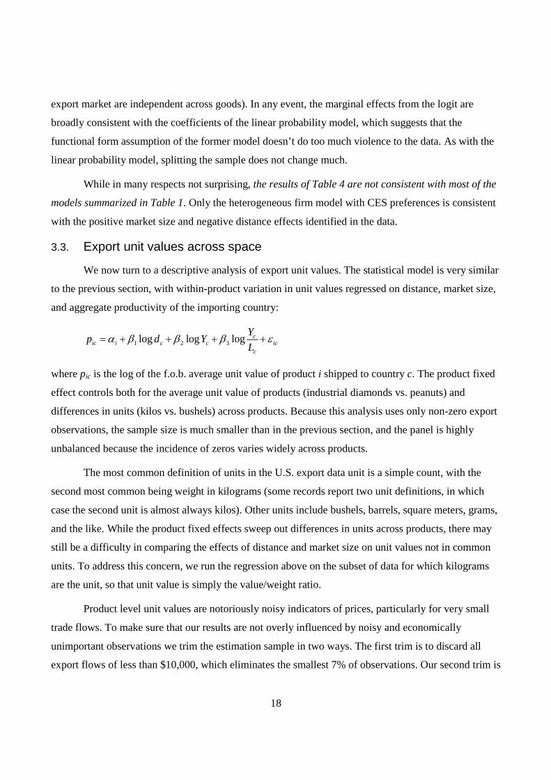
We now turn to a descriptive analysis of export unit values. The statistical model is very similar

to the previous section, with within-product variation in unit values regressed on distance, market size,

and aggregate productivity of the importing country:

1 2 3log log log cic i c c ic

c

Yp d YL

α β β β ε= + + + +

where pic is the log of the f.o.b. average unit value of product i shipped to country c. The product fixed

effect controls both for the average unit value of products (industrial diamonds vs. peanuts) and

differences in units (kilos vs. bushels) across products. Because this analysis uses only non-zero export

observations, the sample size is much smaller than in the previous section, and the panel is highly

unbalanced because the incidence of zeros varies widely across products.

The most common definition of units in the U.S. export data unit is a simple count, with the

second most common being weight in kilograms (some records report two unit definitions, in which

case the second unit is almost always kilos). Other units include bushels, barrels, square meters, grams,

and the like. While the product fixed effects sweep out differences in units across products, there may

still be a difficulty in comparing the effects of distance and market size on unit values not in common

units. To address this concern, we run the regression above on the subset of data for which kilograms

are the unit, so that unit value is simply the value/weight ratio.

Product level unit values are notoriously noisy indicators of prices, particularly for very small

trade flows. To make sure that our results are not overly influenced by noisy and economically

unimportant observations we trim the estimation sample in two ways. The first trim is to discard all

export flows of less than $10,000, which eliminates the smallest 7% of observations. Our second trim is

19

to look only at flows where the data reports a count (as in, “number of cars” or “dozens of pairs of

socks”), and to discard all observations with a count of one. Since there are almost no products where

both a count and kilos are reported, we do not analyze this subset of data.

Table 5 reports the results of our export unit value regressions. A striking message is that

distance has a very large positive effect on unit values. For manufactured goods, compared to the

excluded Canada/Mexico category, small distances (less than 4000km) increase unit values by 16 log

points, while larger distances increases unit values by 60-70 log points, which is a factor of about 2.

For goods where units are reported in kilos, so that unit value is also value/weight, the effect of small

distance is somewhat larger at 26 log points, while the effect of larger distances is about the same as for

manufactured goods. For the subset of goods where units are a count, and the count is greater than 1,

results are broadly similar.

Table 5 also shows that market size has a small but statistically significant negative effect on

export unit values of manufactured goods, with an elasticity of -0.06 when small values are excluded.

This effect is also apparent when nonmanufactured goods are pooled with manufactured goods. For

goods measured in kilos the effect is zero when small values are excluded. The effect of aggregate

productivity is fragile: there is a small positive effect when the sample is restricted to products

measured in kilos, while it is either zero and or small and negative in other sub samples.

The strong positive relationship between export unit values and distance seen in Table 5 is

inconsistent with all of the models presented in section 2. The baseline monopolistic competition

model predict a zero relationship, while the other models predict a negative relationship between export

unit values and distance, the exact opposite of what shows up so strongly in the data. Only the Melitz-

Ottaviano model is consistent with the negative market size effect on prices.

3.4. Variable trade costs and zeros

Table 3 shows conclusively that zeros are increasing in distance. If variable trade costs are

increasing in distance, then this result is consistent with all of the models except the baseline

monopolistic competition model, which is a bit of a straw man in light of Table 2. Nonetheless, the

evidence of Table 3 is only indirect, since it does not include direct measures of trade costs. In this

section we use more direct evidence on falling variable trade costs to confirm their importance in

explaining zeros.

20

Shipping costs are probably the largest component of variable trade costs (other components

include the cost of insurance and the interest cost of goods in transit). While most observers take it for

granted that shipping costs have fallen dramatically since World War II, hard data is surprisingly

difficult to come by and the trends are ambiguous when the data is analyzed (Hummels, 1999).

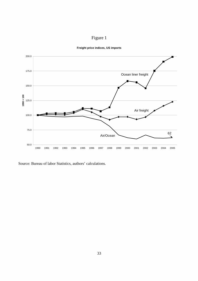
However, there is no doubt that the relative cost of air shipment has declined precipitously. Hummels

(1999) shows the decline in air shipment costs to 1993, though Hummels’ data (as he notes) is not a

price index. Since 1990, the U.S. Bureau of Labor Statistics has been collecting price indices on the

transport costs borne by U.S. imports. Figure 1 uses this data to illustrate that between 1990 and 2005,

the relative price of air to ocean liner shipping for U.S. imports fell by nearly 40%, continuing the trend

documented by Hummels (1999). As illustrated in the figure, this drop in the relative price of air

shipment is partly due to the increasing nominal cost of ocean liner shipping, and partly due to a drop

in the nominal price of air shipment. Micco and Serebrisky (2006) show that the drop in air shipment

rates is partly due to economic policy: the United States implemented a series of “Open Skies

Agreements” between 1990 and 2003 which reduced nominal air transport costs by 9%. There is no

comparable data on the price of shipping by train and truck, modes used exclusively on imports from

Canada and Mexico. The BLS also reports a price index for air freight on exports, but does not report a

price index for ocean liner shipping on exports. Not surprisingly, there is no trend in the relative price

of air shipping for imports and exports. In what follows we assume that the trend illustrated in Figure 1

holds for exports as well.

The fall in the relative price of air shipment since 1990 implies that products shipped by air saw

a fall in their variable trade costs compared to products shipped by ocean liner. This has direct

implications for the incidence of export zeros: export zeros should have disappeared more often for air

shipped than for surface shipped goods. We test this implication with a simple but powerful

differences-in-differences empirical strategy.

The data used in this section is 6-digit HS U.S. exports for 1990 and 2005. We use HS6 rather

than the more disaggregated HS10 data of the previous sections because HS10 definitions change

frequently, making an accurate match of products over 15 years impossible.13

13 Even using HS6 data we had to discard about 20% of exports by value because of matching problems, mainly having to do with differences in units over time

21

Consider export zeros in 1990. By 2005, some of these zeros have disappeared for various

reasons. Conditional on a good being exported, firms choose the optimal shipment mode, and those

who choose to ship by air benefit from the falling cost of air shipment. If the theory prediction is

correct, then new export flows in 2005 will be more likely when they are shipped by air. Define

xict = exports of product i to country c in year t.

zict = 1 if xict = 0, 0 otherwise.

aict = 1 if exports shipped by air, 0 otherwise

yic = 1 if (zic1990 = 1 and zic2005 = 0), 0 otherwise

The variable yic is an indicator of a new trade flow starting sometime between 1990 and 2005: there

were no exports in 1990, and positive exports in 2005. Note that yic = 0 for three distinct reasons:

a. (zic1990 = 0 and zic2005 = 0) export in both years

b. (zic1990 = 1 and zic2005 = 1) export in neither year

c. (zic1990 = 0 and zic2005 = 1) export in 1990 but not in 2005

An empirical model to explain yic is

( ) ( )2005Pr 1ic i c icy F aα α β= = + +

where F is the normal or logistic cdf, and the α’s are country and product fixed effects. That is, the

probability of a new export depends on country and product effects and the shipment mode in 2005.

Note that since aic2005 is undefined if zic2005 = 1, the statistical model includes observations only on

active trade flows in 2005, and compares the characteristics of new flows (yic = 1) versus old flows (yic

= 0). Under the null β > 0: the new flows are more likely to be sent by air.

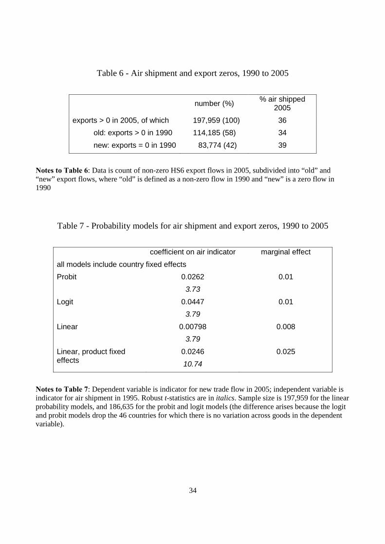
Table 6 summarizes the data. There were nearly 200,000 non-zero HS6 export flows in 2005, of

which more than 40% were zeros in 1990. Of these “new” trade flows, 39% were shipped by air,

compared to 34% shipped by air among “old” flows. Thus there is a 5 percentage point difference in

the likelihood of air shipment for new flows.

Given all the other changes in the global economy since 1990, Table 6 is certainly not definitive

evidence of the importance of falling variable trade costs in explaining disappearing export zeros.

Table 7 reports estimates of the dichotomous probability model above. For technical reasons it is not

22

possible to estimate two-way logit or probit fixed effects models with product indicators, so the first

three rows of the Table report results with country effects only. The final row of the Table is the most

interesting, since it includes country and product fixed effects. The effect of air shipment is precisely

estimated: exports shipped by air in 2005 are 2.5 percentage points more likely to be new. This is a

substantial effect compared to the overall share of new exports in 2005 (42 percent), so that the air

shipment dummy accounts for almost 6 percent of new trade flows in 2005.

We conclude from this section that higher variable trade costs increase the incidence of export

zeros.

4. TRADE WITH HETEROGENEOUS QUALITY The empirical evidence presented above has a clear message: the Melitz (2003) model extended

to multiple asymmetric countries does a good job of explaining export zeros, but can not explain spatial

variation in prices. By contrast, the predictions of the Eaton-Kortum, monopolistic competition, and

Melitz-Ottaviano models are inconsistent with both zeros and spatial price variation. In this section we

build a model that has the virtues of the asymmetric HFT model without this vice. Since firms compete

on the basis of quality as well as price in the model, we refer to it as the quality heterogeneous firms

model, QHFT for short14. In supposing that firms compete on quality as well as price, we follow a

number of important recent papers, including Schott (2004), Hummels and Klenow (2005), and Hallak

(2006) among others.

Most of the assumptions and notation are as in section 2.3 above. There are two main changes –

one on the demand side – consumers now care about quality – and one on the supply side – firms

produce varieties of different quality. More precisely, consumers regard some varieties as superior to

others. This superiority could be regarded purely as a matter of taste, but we will interpret superiority

as a matter of “quality.” The utility function is

14 A recent paper, Helble and Okubo (2006), independently develops a different model of trade with heterogeneous quality.

23

( ) 1;)()/11/(1/11 >=

−

Θ∈

−∫ σσσ

i ii diqcU (13)

where c and q are the quantity and quality of a typical variety and Θ is the set of consumed varieties.

The corresponding expenditure function for nation-d is

1/(1 )1 1( ) ( )( ) ( ) ;

( ) ( )d d

d d d d j

p j p jp j c j B P djq j q j

σσ σ −− −

∈Θ

⎛ ⎞⎛ ⎞ ⎛ ⎞⎜ ⎟= ≡⎜ ⎟ ⎜ ⎟⎜ ⎟⎝ ⎠ ⎝ ⎠⎝ ⎠∫ (14)

where p(j)/q(j) has the interpretation of a quality-adjusted price of good-j, P is the CES index of

quality-adjusted prices, and Θ the set of consumed varieties; Bd is defined as above. The standard CES

preferences are a special case of (13) with q(j)=1, for all j.

As in the standard HFT model, manufacturing firms draw their a from a random distribution

after paying a fixed innovation cost of FI units of labor. In the QHFT model, however, high costs are

not all bad news, for higher quality is assumed to be come with higher marginal cost. In particular

( ) 1,)()( 1 −>= + θθjajq (15)

where 1 + θ is the ‘quality elasticity’, namely the extent to which higher marginal costs are related to

higher quality (setting θ = -1 reduces this to the standard HFT model).

At the time it chooses prices, the typical firm takes its quality and marginal cost as given, so the

standard Dixit-Stiglitz results apply. Mill-pricing with a constant mark-up, σ/(σ-1), is optimal for all

firms in all markets and this means that operating profit is a constant fraction, 1/σ , of firm revenue

market by market. Using (15) in (14), operating profit for a typical nation-o firm selling in nation-d is

(1 )( )1 1/

o dw a j Bθ σ

σ σ

−⎛ ⎞⎜ ⎟−⎝ ⎠

(16)

The only difference between this and the corresponding expression for profits without quality

differences is the θ in the exponent. Plainly, the properties of this model crucially depend on how

elastic quality is with respect to marginal cost. For [ )1,0θ ∈ − , quality increases slowly with cost and

the optimal quality-adjusted consumer price, namely ( )od ow a θφ − , increases with cost. In this case, a

firm’s revenue and operating profit fall with its marginal cost. For 0θ > , by contrast, quality increases

24

quickly enough with cost so that the quality-adjusted price falls as a rises, so higher a’s are associated

with higher operating profit. Henceforth we focus on the 0θ > case because, as the empirics above

suggested, it is the case that is most consistent with the data.

With (16), the cut-off condition for selling to typical market-d is ( ) (1 )od o od dw a B fθ σφ − = ,

which can be rewritten as

1( 1)

od do od

Bw af

θ σφ −⎡ ⎤= ⎢ ⎥⎣ ⎦

(17)

Assuming 0θ > , this tells us that only firms with sufficiently high-price/high-quality goods find it

worthwhile to sell to distant markets. This is the opposite of Melitz (2003) and all other HFT models.

In standard HFT models, competition depends only on price, so it is the lowest priced goods that make

it to the most distant markets. In the QHFT model, competition depends on quality-adjusted prices and

with θ > 0, the most competitive varieties are high-price/high-quality. This means that distance selects

for high-priced varieties rather than low-priced variety as in the HFT model.

4.1. Quality HFT’s spatial pattern of zeros and prices

The spatial pattern of zeros in the QHFT model conforms to those of the HFT model, as a

comparison of the cut-off conditions of the two models, (9) and (17), reveals. The key, new implication

has to do with the relationship between prices and distance. Since a high price indicates high

competitiveness (quality-adjusted price falls as the price rises), the marginal cost thresholds are

increasing in distance, rather than decreasing as in the HFT model. Given that mill pricing is optimal,

this means that both landed (c.i.f.) and shipping (f.o.b.) prices increases with the distance between trade

partners. (See the Appendix for the exact relationship.)

Thus, average f.o.b. prices are increasing in distance. This is consistent with the evidence

presented in Section 3. Finally, we note that the logic of the model is that average f.o.b. quality-

adjusted prices are decreasing in distance, but since the data report only average unit values this is not a

testable implication. Equation (17) also implies that the relationship between average f.o.b. prices and

market size is decreasing, the opposite of the relationship given by (12) in the baseline asymmetric

HFT model. The reason for the different prediction is that as export market size increases lower quality

firms will find it profitable to enter, which lowers average f.o.b. price in larger markets.

25

We summarize the quality HFT model’s predictions as

Export zeros The probability of an export zero is increasing in bilateral distance, and

decreasing in market size.

Export prices Considering a single product sold by o in multiple destinations, the f.o.b price is

increasing in the distance between o and d. The effect of market size on average

f.o.b. price is negative in the baseline model.

These predictions are noted in the last line of Table 2. Once again, the QHFT model is the only one that

we considered which matches the findings of the data analysis in Section 3.

5. CONCLUDING REMARKS This paper has shown that existing models of bilateral trade all fail to explain key features of

the product-level data. In particular, the well-known models of Eaton and Kortum (2002), Melitz

(2003) and Helpman and Krugman (1985) all fail to match at least some of the following facts, which

we document using product-level U.S. trade data:

• Most products are exported to only a few destinations.

• The incidence of these “export zeros” is positively related to distance and negatively related to

market size.

• The average unit value of exports is positively related to distance.

We also show that falling air shipment costs are related to the disappearance of export zeros.

We finish the paper by proposing a modification to Melitz’ (2003) model which fits all of the

facts just summarized. In this new model, firms compete on quality as well as price, and differ in their

relative location.

26

REFERENCES Alvarez, Fernando, and Robert E. Lucas Jr., 2005, “General Equilibrium Analysis of the Eaton-Kortum

Model of International Trade”, NBER Working Paper 11764 (November). Axtell, Robert L., 2001, “Zipf Distribution of U.S. Firm Sizes”, Science 293(5536): 1818 - 1820

(September 7).

Baldwin, Richard, 2005, “Heterogeneous firms and trade: testable and untestable properties of the Melitz model”, NBER Working Paper 11471 (June).

Bernard, Andrew B., Jonathan Eaton, J. Bradford Jensen, and Samuel Kortum, 2003, “Plants and Productivity in International Trade”, American Economic Review 93(4): 1268-1290 (September).

Besedeš , Tibor, and Thomas J. Prusa (2006a), “Ins, outs, and the duration of trade” Canadian Journal of Economics 39(1): 266–295.

Besedeš , Tibor, and Thomas J. Prusa (2006b), “Product differentiation and duration of US import trade” Journal of International Economics 70(2): 339-358.

Choi, Yo Chul, David Hummels, and Chong Xiang, 2006, “Explaining Import Variety and Quality: The Role of the Income Distribution”, NBER Working Paper 12531 (September).

Deardorff, Alan V., 1998, "Determinants of Bilateral Trade: Does Gravity Work in a Neoclassical World?", in Jeffrey A. Frankel, Ed., The Regionalization of the World Economy, Chicago: University of Chicago Press for the NBER, 7-22.

Deardorff, Alan, 2004, "Local Comparative Advantage: Trade Costs and the Pattern of Trade", University of Michigan RSIE Working paper no. 500.

Demidova, Svetlana, 2006, “Productivity Improvements and Falling Trade Costs: Boon or Bane?,” http://demidova.myweb.uga.edu/research.html.

Eaton, Jonathan and Samuel Kortum, 2002, “Technology, Geography, and Trade”, Econometrica 70(5): 1741-1779 (September).

Eaton, Jonathan, Samuel Kortum and Francis Kramarz (2005). “An Anatomy of International Trade: Evidence from French Firms,” October version.

Falvey, Rod, David Greenaway, and Zhihong Yu, 2006,. “Extending the Melitz Model to Asymmetric Countries,” University of Nottingham GEP Research Paper 2006/07.

Feenstra, Robert C., James R. Markusen, and Andrew K. Rose, 2001, “Using the gravity equation to differentiate among alternative theories of trade” Canadian Journal of Economics 34 (2): 430-447 (May).

Feenstra, Robert C.; and Andrew K. Rose, 2000, “Putting Things in Order: Trade Dynamics and Product Cycles”, Review of Economics and Statistics 82(3): 369-382.

Hallak, Juan Carlos, 2006, “Product Quality and the Direction of Trade”, Journal of International Economics 68(1): 238-265.

27

Harrigan, James, 2003, “Specialization and the Volume of Trade: Do the Data Obey the Laws?” in Handbook of International Trade, edited by James Harrigan and Kwan Choi, London: Basil Blackwell.

Harrigan, James, 2006, “Airplanes and comparative advantage”, revision of NBER Working Paper 11688.

Haveman, Jon and David Hummels, 2004, “Alternative hypotheses and the volume of trade: the gravity equation and the extent of specialization”, Canadian Journal of Economics 37 (1): 199-218 (February).

Helble, Mathias, and Toshihiro Okubo, 2006, “Heterogeneous quality and trade costs,” HEI mimeo, Geneva.

Helpman, Elhanan and Paul Krugman, 1985, Market Structure and Foreign Trade, Cambridge, MA: MIT Press.

Helpman, Elhanan, Marc Melitz, and Stephen Yeaple, 2004, “Export Versus FDI with Heterogeneous Firms”, American Economic Review 94(1): 300-316.

Helpman, Elhanan, Marc Melitz, and Yona Rubinstein, 2007, “Estimating Trade Flows: Trading Partners and Trading Volumes”, NBER Working Paper 12927.

Hummels, David, 1999, “Have International Transportation Costs Declined?”, http://www.mgmt.purdue.edu/faculty/hummelsd/

Hummels, David, and Peter Klenow, 2005, “The Variety and Quality of a Nation’s Exports”, American Economic Review 95(3): 704-723 (June).

Melitz, Marc, 2003, “The impact of trade on intraindustry reallocations and aggregate industry productivity”, Econometrica 71(6): 1695-1725 (November).

Melitz, Marc and Gianmarco Ottaviano, 2005, “Market Size, Trade, and Productivity”, revision of NBER Working Paper No. 11393.

Micco, Alejandro and Tomas Serebrisky, 2006, “Competition regimes and air transport costs: The effects of open skies agreements”, Journal of International Economics 70(1): 25-51 (September).

Ottaviano G., T. Tabuchi, and J. Thisse, 2002, “Agglomeration and Trade Revisited” International Economic Review 43(2): 409-436 (May).

Schott, Peter K., 2004, “Across-product versus within-product specialization in international trade”, Quarterly Journal of Economics 119(2):647-678 (May).

Yeaple, Stephen Ross, 2005, “A simple model of firm heterogeneity, international trade, and wages.” Journal of International Economics 65(1): 1-20.

28

Table 1 - Summary of model predictions

Pr(export zero) f.o.b. export price

distance importer size distance importer

size

Eaton-Kortum

+ + - 0

Monopolistic competition, CES n/a n/a 0 0

Monopolistic competition, linear demand + 0 - 0

Heterogeneous firms, CES

+ - - +

Heterogeneous firms, linear demand + + - -

Heterogeneous firms, quality competition

+ - + -

Notes to Table 1 The first five rows of the table summarize the theoretical comparative static predictions discussed in Section 2, with the last row giving the predictions of the model that we develop in Section 4. The six models under discussion are listed in the first column. Each entry reports the effect of an increase in distance or importer size on the probability of an export zero or f.o.b. export price. An export zero is defined to occur when a country exports a good to one country but not all.

29

Table 2 - Incidence of zeros in U.S. trade, 2005

Imports Exports all countries

Trading partners 228 230 HS10 products 16,843 8,880

partners × products 3,840,204 2,042,400

percent zeros 92.6 82.2 100 largest countries

HS10 products 16,843 8,880

partners × products 1,684,300 888,000

percent zeros 85.5 70.0

30

Table 3 - Countries classified by distance from United States country km country km country km country km Canada 0 Mexico 0 7800-14000km 1-4000km Burkina.Faso 7908 Japan 10910 Jamaica 2326 Costa.Rica 3300 Bulgaria 7920 China 11154 DominicanRep 2376 Venezuela 3317 Romania 7985 Korea 11174 Belize 2670 Panama 3341 Chile 8079 Pakistan 11389 Honduras 2936 Barbados 3345 Niger 8146 Yemen 11450 El.Salvador 3049 TrinidadTobago 3501 Cote.D'Ivour 8175 Ethiopia 11530 Guatemala 3110 Colombia 3829 Greece 8261 Rwanda 11629 Nicaragua 3115 Argentina 8402 Burundi 11670 4000-7800km Uruguay 8488 Uganda 11679 Ecuador 4357 Gambia 6535 Ghana 8488 India 12051 Iceland 4518 Switzerland 6607 Togo 8572 Kenya 12152 Ireland 5448 Sweden 6641 Benin 8669 Nepal 12396 Peru 5671 Guinea.Bissau 6730 Turkey 8733 Zambia 12400 Portugal 5742 Brazil 6799 Nigeria 8737 South.Africa 12723 United.Kingdom 5904 Algeria 6800 Chad 9351 Tanzania 12759 Spain 6096 Finland 6938 Egypt 9358 Malawi 12781 Morocco 6109 Guinea 7050 Syria 9445 Zimbabwe 12835 France 6169 Austria 7130 Israel 9452 Bangladesh 12943 Netherlands 6198 Poland 7183 Jordan 9540 Hong.Kong 13129 Belgium-Lux 6221 Italy 7222 Cameroon 9622 Mozambique 13428 Bolivia 6235 Mali 7328 Gabon 9686 Comoros 13442 Norway 6238 Hungary 7344 Iran 10190 Philippines 13793 Senegal 6379 Tunisia 7347 Congo 10515 Germany 6406 Paraguay 7421 over 14000km Denmark 6518 New.Zealand 14098 Mauritius 15224 Thailand 14169 Malaysia 15350 Madagascar 14291 Australia 15958 Sri.Lanka 14402 Indonesia 16371 Seychelles 15095

31

Table 4 - Statistical determinants of non-zero U.S. exports, 2005

linear probability model random effects probit model coefficient t-statistic marginal eff. t-statistic full sample

1 < km ≤ 4000 -0.079 -1.34 0.040 9.74

4000 < km ≤ 7800 -0.335 -5.90 -0.238 -67.6

7800 < km ≤ 14000 -0.341 -5.41 -0.273 -65.4

14000 < km -0.316 -4.74 -0.160 -63.5

landlocked -0.017 -0.63 -0.036 -21.4

log real GDP 0.080 10.8 0.101 90.9

log real GDP/worker 0.054 3.92 0.087 80.9

manufactured goods only

1 < km ≤ 4000 -0.021 -0.33 0.072 11.3

4000 < km ≤ 7800 -0.295 -4.75 -0.268 -56.3

7800 < km ≤ 14000 -0.311 -4.55 -0.311 -55.1

14000 < km -0.287 -3.86 -0.196 -55.1

landlocked -0.018 -0.65 -0.041 -17.6

log real GDP 0.086 11.3 0.121 87.9

log real GDP/worker 0.062 4.13 0.103 75.8

Notes to Table 4: Dependent variable is indicator for non-zero exports of HS10 products. Independent variables are characteristics of U.S. export destinations. Estimator for linear probability model is OLS, with HS10 product fixed effects and errors clustered by country. Estimator for random effecst probit is maximum likelihood, with product random effects and errors not clustered by country. Panel dimensions are 8,800 products and 100 countries for full sample, 5,834 products and 100 countries for manufactured goods only sample. R2 within = 0.28 for linear probability model in the full sample, R2 within = 0.31 in manufactured goods only sample.

32

Table 5 - Statistical determinants of U.S. export unit values, 2005 unrestricted sample value ≥ $10,000 number ≥ 2

all manuf. kilos all manuf. kilos all manuf.

1 < km ≤ 4000 0.182

2.51

0.160

1.64

0.263

4.66

0.185

2.63

0.161

1.65

0.273

5.41

0.207

1.78

0.209

1.81

4000 < km ≤ 7800 0.664

12.2

0.713

9.01

0.687

19.1

0.608

11.8

0.665

8.64

0.600

19.4

0.774

7.77

0.777

7.85

7800 < km ≤ 14000 0.594

10.2

0.647

7.65

0.614

17.8

0.547

9.90

0.612

7.43

0.535

19.1

0.688

6.37

0.690

6.42

14000 < km 0.584

10.3

0.651

7.48

0.606

15.2

0.523

9.91

0.591

7.14

0.527

13.1

0.683

5.91

0.686

5.93

landlocked 0.098

1.03

0.032

0.34

0.250

2.73

0.117

1.19

0.057

0.56

0.252

2.76

-0.060

-0.52

-0.060

-0.52

log real GDP -0.063

-4.65

-0.076

-4.63

-0.029

-2.54

-0.047

-3.56

-0.062

-3.79

-0.004

0.34

-0.098

-4.97

-0.098

-5.00

log real GDP/ worker

-0.007

-0.26

-0.043

-1.25

0.093

3.95

0.006

0.23

-0.030

-0.89

0.111

5.38

-0.110

-2.64

-0.109

-2.62

R2 within 0.028 0.029 0.047 0.027 0.029 0.052 0.029 0.029

num. products 7,880 4,908 4,626 7,831 4,886 4,582 2,370 2,322

number of obs 218,025 150,077 112,537 181,020 123,547 92,085 87,902 87,268

Notes to Table 5: Dependent variable is log unit value of exports by HS10 product and export destination. Independent variables are characteristics of export destinations. Estimator is OLS, with HS10 product fixed effects and errors clustered by country. t-statistics in italics. See text for discussion of different subsamples.

33

Figure 1

Freight price indices, US imports

50.0

75.0

100.0

125.0

150.0

175.0

200.0

1990 1991 1992 1993 1994 1995 1996 1997 1998 1999 2000 2001 2002 2003 2004 2005

1990

= 1

00

Ocean liner freight

Air freight

Air/Ocean62

Source: Bureau of labor Statistics, authors’ calculations.

34

Table 6 - Air shipment and export zeros, 1990 to 2005

number (%) % air shipped 2005

exports > 0 in 2005, of which 197,959 (100) 36 old: exports > 0 in 1990 114,185 (58) 34 new: exports = 0 in 1990 83,774 (42) 39

Notes to Table 6: Data is count of non-zero HS6 export flows in 2005, subdivided into “old” and “new” export flows, where “old” is defined as a non-zero flow in 1990 and “new” is a zero flow in 1990

Table 7 - Probability models for air shipment and export zeros, 1990 to 2005

coefficient on air indicator marginal effect all models include country fixed effects Probit 0.0262

3.73 0.01

Logit 0.0447 3.79

0.01

Linear 0.00798 3.79

0.008

Linear, product fixed effects

0.0246 10.74

0.025

Notes to Table 7: Dependent variable is indicator for new trade flow in 2005; independent variable is indicator for air shipment in 1995. Robust t-statistics are in italics. Sample size is 197,959 for the linear probability models, and 186,635 for the probit and logit models (the difference arises because the logit and probit models drop the 46 countries for which there is no variation across goods in the dependent variable).

35

Appendix for “Zeros, quality and space: Trade theory and trade evidence”

by Richard Baldwin and James Harrigan, June 2007.

This appendix provides a more complete treatment of the models discussed in the paper.

5.1. Comparative advantage: Eaton-Kortum

The slightly simplified version of the Eaton-Kortum (EK) model that we work with has C nations each

of which is endowed with a single factor of production (labor) used to produce a continuum of goods

under conditions of perfect competition and constant returns. The transport costs between a typical

origin nation (nation-o) and a typical destination nation (nation-d) are assumed to be of the iceberg type

and captured by the parameters τod ≥ 1 where τod is the amount of the good that must be shipped from o

to sell one unit in d. The double-subscript notation follows the standard ‘from-to’ convention, so τoo = 1

for all nations (intra-nation trade costs are zero). Consumer preferences are identical across nations and

defined over the continuum of goods. They are described by a CES utility function, and expenditure on

any given variety by a typical destination nation (nation-d) is

( ) ( )1

11 1

1( ) ( ) ( ) ; , ( )dd d d d d d d

d j

Ep j c j p j B B P p j djP

σσ σ

σ

−− −

−∈Θ

⎛ ⎞= ≡ ≡ ⎜ ⎟⎜ ⎟

⎝ ⎠∫ (A1)

where cd(j) and pd(j) are nation-d’s consumption and consumer price of good-j, Pd is the ideal CES

price index, Ed is total expenditure (GDP in equilibrium), and σ is the elasticity of substitution among

varieties. Without loss of generality, we order product indices such that the set of available goods Θ

equals the unit interval.

Each nation’s manufacturing technology – its’ vector of unit labor input coefficients – comes

from a stochastic technology-generation process much like the one used later by Melitz (2003). In the

EK model, this exogenous process is costless and realizations are drawn before the analysis opens.

Denoting nation-o’s unit labor coefficient for good-j as ao(j), the model assumes that each ao(j) is an

independent draw from the nation-specific cumulative distribution function (cdf)15

15 EK work with firm productivity as the random variable rather than the standard Ricardian labour input coefficient, namely z =1/a, so their cdf is exp(-T/zθ).

36

0,1][ ≥−= − aeaF aTo

oθ

(A2)

where To > 0 is a technology parameter that differs across countries. The expectation of ao(j) is

1/ 11T θ

θ− ⎡ ⎤Γ +⎢ ⎥⎣ ⎦

, where Γ is the gamma function, so To can be thought of as nation-o’s average absolute

advantage parameter, i.e. its technology level. Importantly, the draws are independent across goods and

nations.

Although all nations can make all goods, perfect competition means only the lowest cost

supplier actually sells in destination d. The price that each nation-o could offer for good-j in destination

nation-d is:

)()( jawjp ooodod τ= (A3)

where wo and ao(j) are nation-o’s wage and unit labor coefficient in good-j, respectively. Perfect

competition implies that the equilibrium price for good-j in nation-d satisfies:

1...( ) min ( )d o C od o op j w a jτ== (A4)

Finding comparative advantage

The next step is to find the probability that a particular nation is the lowest cost supplier in a particular

good in a particular market. This task involves a series of probability calculations that use two

implications of (A2) and (A3). First, the cdf of pcd(j) is [ ] 1 exp( )cd cdG p p Tθ= − − where

( )cd c c cdT T w θτ −≡ .16 Thus the probability that pcd(j) > k equals exp( )cdk Tθ− . Second, pod(j) is lower than

the offer price of all other nations with probability 1 minus the probability that all other prices are

higher. Since all draws of the a’s are independent across nations, the probability that all other prices are

higher is ( )exp cd cdc o

p Tθ≠

−∏ , which simplifies to exp od cdc o

p Tθ

≠

⎛ ⎞⎛ ⎞−⎜ ⎟⎜ ⎟

⎝ ⎠⎝ ⎠∑ . Since pod(j) is just one of many

offer-prices that nation-o may have drawn, we must integrate over all possible pod(j), weighting each by

16 Dropping subscripts where clarity permits, ( ) ( )Pr Pr Pr 1 expk kp k aw k a Tw w

θ

ττ τ

⎛ ⎞⎛ ⎞ ⎛ ⎞≤ = ≤ = ≤ = − −⎜ ⎟⎜ ⎟ ⎜ ⎟⎜ ⎟⎝ ⎠ ⎝ ⎠⎝ ⎠, where k is an

arbitrary price level. Noting that this holds for all k and the supports of p and a are identical, we get the result in the text.

37

its probability. Thus the probability of nation-o having a comparative advantage in good-j in market d

is 0

exp [ ]od cd odc o

p T dG pθ∞

≠

⎛ ⎞⎛ ⎞−⎜ ⎟⎜ ⎟⎝ ⎠⎝ ⎠∑∫ where [ ] 1 exp( )od odG p p Tθ= − − . Solving the integral,

1

;C

odod d cd

cd

T Tπ=

= ∆ ≡∆ ∑ (A5)

Here πod is the probability that nation-o exports any given good-j to nation-d. Since the technology

draws are independent across goods, πod applies to each of the continuum of goods j∈[0,1]. Notice that

∆d is akin to the inverse of the remoteness variable in standard gravity equations, i.e. it is an inverse

index of the distance between nation-d and its trade partners, assuming that trade costs rise with

distance.

Given the complexity of the model, it is remarkable that the expression for ‘stochastic

comparative advantage’, πod, is so simple and intuitive. Thinking of the Tid’s as the expected

competitiveness of nation-i’s goods in nation-d’s market, the probability that nation-o is the most

competitive in any given good is just the ratio of nation-o’s expected competitiveness to that of the sum

of all nations. Notice that the probability πod falls as the bilateral trade costs rises but rises with nation-

o’s average absolute advantage parameter, To. As we shall see, expression (A5) is the key to

characterizing the spatial pattern of zeros in the EK model.

Finding the equilibrium prices

To characterize the predictions for the spatial pattern of prices, we draw on two further implications of

(A2) and (A3). First, with all draws independent across nations, the probability that we have pcd(j) > k

for all origin-nations equals ( )1

expC

cdc

k Tθ=

−∏ , which simplifies to ( )exp dkθ− ∆ . Second, the probability

of at least one nation having a pcd(j) < k is 1 minus the probability that pcd(j) > k for all nations, or

( )1 exp dkθ− − ∆ .17

17 ( )Pr 1 1 exp expc ccd

c cd c cd

T k T kp kw w

θ θ

τ τ⎛ ⎞⎛ ⎞ ⎛ ⎞− −

> = − − =⎜ ⎟⎜ ⎟ ⎜ ⎟⎜ ⎟⎝ ⎠ ⎝ ⎠⎝ ⎠. Since the draws are independent, the joint probability that they are

all higher is 1

expC

c

c c cd

T kw

θ

τ=

⎛ ⎞−⎜ ⎟⎝ ⎠

∏ . Simplification yields the result in the text.

38

Since we do not know each nation’s actual a’s, we cannot determine the price for any given

good. Rather we find the distribution of the prices nation-d pays for a typical good. Due to competition,

the price paid – i.e. the equilibrium price – is the lowest offer price as described by (A4). By definition,

the cdf that describes the equilibrium price gives the probability that the equilibrium price is less than

or equal to any particular level. To find the distribution that describes this ‘lowest price’, we use

[ ] 1 exp( )cd cdF p p Tθ= − − and the independence of prices across goods and suppliers. Specifically, the

probability that all pod(j)’s are greater than an arbitrary level pd is ( )exp d dp θ− ∆ , so the probability that

at least one pod(j) is below pd is ( )1 exp d dp θ− − ∆ . This holds for all possible pd and for any good-j so

the nation-specific distribution that describes the equilibrium price for any good is

( )[ ] 1 expd dG p pθ= − − ∆ (A6)

Because each good’s a is identically and independently distributed, Gd[p] describes the price

distribution for any nation-d, d=1,…,C for any good j ∈ [0,1].

Using (A1), (A6) and switching the variable of integration, it is easy to find the equilibrium CES price

index for nation-d, namely σ−1dP which is defined as ( )1( )di

p i diσ

θ

−

∈∫ . As noted, we cannot determine

the equilibrium price of any given good-j, but we know its cdf to be (A6). Moreover, with a continuum

of varieties (which implies an infinite number of draws from Gd[p]), we know that the distribution of

equilibrium prices across all varieties is identical to the underlying distribution Gd[p] for any given

variety. This means that σ−1dP equals 1

0[ ]dp dG pσ∞ −∫ . Solving the integral

1/(1 )1/ 1

d dPσ

θ σ θθ

−− − +⎛ ⎞⎡ ⎤= ∆ Γ⎜ ⎟⎢ ⎥⎣ ⎦⎝ ⎠

(A7)

where the term in large parenthesis is the gamma function. This makes sense assuming the regularity

condition 1 - σ + θ > 1 holds.

The final task is to determine the distribution of prices for the goods that nation-o exports to

nation-d. Since the probability of nation-o exporting any particular good to nation-d is πod for all

goods, the goods that nation-o actually exports to d is a random sample of all the goods that d buys.

Thus, Gd[p] also describes the cross-good distribution of the prices for the exports from every origin

39

nation to nation-d. This elegant and somewhat surprising result follows from the fact that it is

competition inside nation-d that determines prices, not the characteristics of any particular exporting

nation. Successful exporting countries sell a large number of goods but do not on average charge lower

prices. As we shall see, this result is the key to characterizing the spatial price implications in the EK

model.

Linking export probability to observables

It is impossible to explicitly solve the EK model for general trade costs. The reason is that all nations’

wages enter the system non-linearly, so we cannot use market clearing conditions to determine what

wage a nation must have in order to sell all its output. More specifically, every Tcd contains the inverse

of the wage of nation-c. This, together with the form of πod means that each πod is of order C in each

wage. While solutions exist for C ≤ 5, in practice the solution even for a pair of quadratic equations is

typically too complicated to be useful. One can, however, easily find the wages in the case of autarky

and free trade, as EK show. Without explicit solutions for the w’s, we cannot find a closed form

solution for πod and thus we cannot solve the precise pattern of zeros predicted by the model. Although

this is a major drawback for a theoretical investigation, it poses no problems for our empirical work.

We use data from a single exporting nation for a single year so all identification comes from the spatial

variation in the data which occurs regardless of the level of wages.

We can link the Tod’s and thus the πod’s to observable variables that allow estimation of the

impact of distance and destination market-size on the probability of observing a zero. To this end, we

specify the market-clearing condition for each origin nation. The share of nation-d’s total expenditure

on manufactures from nation-o is πod times Ed, where Ed is d’s total expenditure on manufactures.

Rearranging yields a version of EK’s expression 10, namely

dodod EV π= (A8)

where Vod is the value of all exports from nation-o to nation-d, and Ed is nation-d’s expenditure.18

Nation-o’s market clearing condition is the summation of (A8) over all destination nations. Using (A5),

18 Note that this is the expected expenditure of nation-d on nation-o goods, but since o exports an infinite number of goods to d, the realisation will be identical to the expectation by the law of large numbers.

40

the total sales of nation-o to all markets (including its own) equals the value of its total output, Yo i.e.

GDP, when19

1

No

o od d ddo

TY Ew

θ θθ τ − −

=

⎛ ⎞= ∆⎜ ⎟

⎝ ⎠∑ (A9)

Solving (A9) for To/woθ, using the definitions in (A5), and substituting out the ∆’s using (A7), noting

that the gamma functions cancel, we get

o od dod

od d d cd c cc d

Y PE P E P

θ θ

θ θ θ θ

τπτ τ

−

− −

≠

=+∑

(A10)

5.2. Monopolistic competition

Our version of the monopolistic competition model has C countries and a single primary factor L that is

used in the production of differentiated goods (manufactures) whose trade is subject to iceberg trade

costs. Preferences are CES, so expenditure on manufactured good-j in typical nation-d is given by (A1).

Manufactured goods are produced under conditions of increasing returns and Dixit-Stiglitz

monopolistic competition. Unlike the EK model, all firms in all countries face the same unit labor

requirement, a. According to well-known properties of Dixit-Stiglitz monopolistic competition, nation-

o firms charge consumer (i.e. c.i.f.) prices in nation-d equal to 1od o odp w aσ τ

σ=

−. Consequently, the

shipping (f.o.b.) price for any good is the same for every bilateral trade flow. The CES price index for

typical nation-d involves the integral over all prices

1 1

1

C

d cd c cc

P n wσ σφ− −

=

= ∑ , 1 [0,1]od odσφ τ −≡ ∈

where we have, without loss of generality, chosen units such that a = 1-1/σ. The parameter φod reflects

the ‘freeness’ of bilateral trade (φ ranges from zero when τ is prohibitive to unity under costless trade,

i.e. τ = 1). nc is the number of goods produced in c.

5.2.1. Free entry conditions

With Dixit-Stiglitz competition, a typical nation-o firm’s operating profit from selling in market-d is20

19 This is related to EK’s unnumbered expression between their expressions 10 and 11.

41

1 dod o

Bw σφσ

− (A11)

Summing across all C markets, total operating profit of a typical firm in nation-o is 1

1

Co

oc cc

w Bσ

φσ

−

=∑ .

Developing a new variety involves a fixed set-up cost, namely an amount of labor FI (I for

innovation).21 In equilibrium, free entry ensures that the benefit and cost of developing a new variety

match, so the free-entry condition for nation-o is

1

1

C

o oc c o Ic

w B w Fσ φ σ−

=

=∑ (A12)

for all o = 1,…,C. The equilibrating variables here are the per-firm demand shifters Bd and the wage.

5.2.2. Employment condition and National budget constraint

In equilibrium, all labor must be employed. The amount of labor used per variety is Iax F+ , where x is

production of a typical good. Using the demand function, iceberg trade costs and equilibrium prices,

the total production of a typical variety produced in o is 1

( )C

oc o cc

w Bστ −

=∑ . Solving the integral and using

the expression for P, the full employment condition for typical nation-o is:

1

( )C

o oc o c I oc

n w B F Lστ −

=

⎛ ⎞+ =⎜ ⎟⎝ ⎠∑ (A13)

The final equilibrium expression requires that expenditure equals income. Since free entry eliminates

pure profits, all income comes from labor income, and so equals woLo. The national budget constraint is

thus:

o o oE w L= (A14)

5.2.3. Equilibrium

There are three endogenous variable here for each nation, w, n and E and three equilibrium conditions,

the free entry, employment and national budget constraint conditions. As usual, the three equilibrium

20 Operating profit is proportional to firm revenue since the first order condition p(1-1/σ)=a implies (p-a)c, equals pc/σ. 21 To relate this model to the previous one and the next, it is as if a firm must pay FI to take a draw from the technology-generating distribution, but the distribution is degenerate, always yielding a=1-1/σ.

42

conditions – the free entry, employment and national budget constraint conditions – are not

independent since we derived the demand equations imposing individual budget constraints. This

redundancy allows us to drop one equilibrium condition and choose the labor of one nation as the

numeraire.

Unfortunately, it is impossible to solve the model analytically for the same reason the EK model

could not be solved – the wages enter the model in a highly non-linear manner. Specifically, we can use

(A14) to eliminate the E’s and our expression for the price index to get the free entry condition in terms

of the n’s and w’s only. Then we can use mill pricing to express the free-entry condition as

o o Ix w Fσ σ−= , where xo is the output of a typical firm in nation-o, so that the employment condition

becomes /{ ( ( 1) 1)}o o I on L F w σ σ−= − + . This gives us two equations per nation in the n’s and w’s.

However, the w’s enter these equations with non-integer powers and this renders analytic solutions

impossible.

As before, this lack of tractability is not a problem for our empirics since we work with a single

exporter and a single year of data. The key is that given the CES demand structure, the choke-point

price is infinity so every importing nation will buy some of every variety produced by every nation.

Moreover, given Dixit-Stiglitz monopolistic competition, mill pricing is optimal so the export (i.e.

f.o.b.) price should be the same for every destination regardless of transportation costs.

5.2.4. Aside: MC with an ‘outside’ sector

A standard theoretical artifice yields analytic solutions pinning down the wage in all nations. The trick

is to introduce a Walrasian sector whose output is costlessly traded. Assuming nations are similar

enough in size for all nations to produce some of this ‘outside’ good, free trade equalizes wages

globally. Choosing the outside good as numeraire and choosing its units such that its prices equals the

wage, free trade equalizes all wages to unity worldwide. Under this artifice, the free entry condition for

nation-o is

1

C

oc c Ic

B Fφ σ=

=∑ (A15)

43

The equilibrating variables here are the per-firm demand shifters Bd. The C free-entry conditions are

linear in the Bd’s and so easily solved.22 In matrix notation

1IFσ−=B Φ (A16)

where Φ is an C × C matrix of bilateral trade freeness parameters (e.g., the first row of Φ is φ11,…,φ1C),

and B is the C × 1 vector of Bd’s. This shows that the equilibrium B’s depend upon bilateral trade

freeness in a complex manner; all the φ’s affect every B. The complexity can be eliminated by making

strong assumptions on trade freeness, e.g. imposing φod=φ for all trade partners, but we retain arbitrary

φod’s. Importantly, the equilibrium B’s are completely unrelated to market size; they depend only upon

the parameters of bilateral trade freeness. The deep economic logic of this has to do with the Home

Market Effect; big markets have many firms since firms enter until the per-firm demand is unrelated to

market size.23

We can characterize the equilibrium without decomposing the B into their components (E’s and

n’s) but doing so is awkward because the B’s do not map cleanly into real world variables. The natural

equilibrating variable – the mass of firms in each nation, nc – can be extracted from the B’s. Using the

definition of the CES price index, Dixit-Stiglitz mark-up pricing and nation-wise symmetry of

varieties, 1

1

C

d c cdc

P nσ φ−

=

= ∑ . Using this, along with the definition of Bd in (A1), we write the C definitions

of the B’s (with a slight abuse of matrix notation) as ' /=Φ n E B , where n is the C × 1 vector of nc’s

and BE / is defined as (E1/B1, …, EC/BC). Solving the linear system

1 1

1

' ,..., C

C

E EB B

− ⎡ ⎤= ⎢ ⎥

⎣ ⎦n Φ (A17)

Each no directly involves all the φ’s, all the E’s, and all the B’s (each of which involves all the φ’s).

Solutions for special cases are readily available, but plainly the equilibrium n’s are difficult to

characterize for general size and trade cost asymmetries. The complexity of (A17) is the heart of the

difficulties the profession has in specifying the Home Market Effect in multi-country models (see

Behrens, Lamorgese, Ottaviano and Tabuchi 2004). 22 This solution strategy follows Behrens, Lamorgese, Ottaviano and Tabuchi (2004). 23 In the terminology of Chamberlinian competition, the extent of competition rises until the residual demand curve facing each firm (i.e. p-σB) shifts in to the point where each firm is indifferent to entry. Since entry costs are identical in all markets, the residual demand-curve must be in the same position in every market.

44

Notice that under this artifice, an increase in a nation’s L is fully offset by a rise in its n, so it B

remains unaffected. This can happen since labor can be drawn from the outside sector at a constant

wage rate. In the baseline model without the outside good, the rise in L results partly in a rise in n and

partly in a rise in w. Or, to put it differently, the Home Market Effect is much stronger in the model

with the outside good since a rising wage does not dampen the profits of local firms.

5.3. A multi-nation asymmetric HFT model

Our HFT model embraces all of the demand, market-structure and trade cost features of the MC model

above but adds in two new elements – beachhead costs (i.e. fixed market-entry costs) and hetero-

generous marginal costs at the firm level. Firm-level heterogeneity is introduced – as in the EK model –

via a stochastic technology-generation process. When a firm pays its standard Dixit-Stiglitz cost of

developing the ‘blueprint’ for a new variety, FI, it simultaneously draws a unit labor coefficient ‘a’

associated with the blueprint from the Pareto cdf24

00

[ ] , 0aG a a aa

κ⎛ ⎞

= ≤ ≤⎜ ⎟⎝ ⎠

(A18)

After seeing its a, the firm decides how many markets to enter. Due to the assumed Dixit-Stiglitz

market structure, the firm’s optimal price is proportional to its marginal cost, its operating profit is

proportional to its revenue, and its revenue in a particular market is inversely proportional to its relative

price in the market under consideration.

5.3.1. Cut-off conditions

Thus, the cut-off conditions that define the maximum-marginal-cost thresholds for market-entry are

1 1 1; (1 1/ )od d o od oB w a w f f Fσ σ σφ σ σ− − −= ≡ − (A19)

for all o, d = 1,…,N, where F is the beachhead cost (identical all firms in all nations for notational

simplicity). Here Bd is defined as in (A1), and the endogenous aod’s are the cut-off levels of marginal

costs for selling from nation-o to nation-d.

24 The EK and HFT models work well with a broad family of distributions, but the analytics are more transparent with an explicit distribution, e.g. either the Pareto or exponential distributions; the Pareto is traditional in HFT models. This formulation of the randomness differs trivially from Melitz, who, like EK, works firm-level efficiency (i.e. 1/a).

45

5.3.2. The free entry conditions

From the cut-off conditions, we know that not all blueprints will be produced. Thus the mass of

blueprints in typical nation o – what we call mo – exceeds the mass of produced varieties – what we call

no in line with standard MC model notation. Usual Dixit-Stiglitz results imply that the mass of

blueprints rises to the point where potential entrants are just indifferent to sinking the development

costs woFI and taking a draw from the technology-generating distribution (A18).

A potential entrant in o knows the various a’s that may be drawn will result in different levels

of operating profit. Before paying woFI to take a draw from (A18), the firm forms an expectation over

all possible draws using its knowledge of the thresholds defined by (A19). The expected value of

drawing a random a is ( )( )11 1

01

( ) [ ] / 1 1/odC a

od d o od

B w a w f dG a σσ σφ σ σ −− −

=

− −∑∫ . Here each term in the sum

reflects the expected operating profit from selling to a particular market (net of the beachhead cost)

taking account of the fact that the firm only finds it profitable to sell to the market if it draws a

marginal cost below the market-specific threshold marginal cost, aod. Potential entrants are indifferent

to taking a draw when this expectation just equals the set-up cost, woFI, so the free-entry conditions

hold when 1 1 1

01

( ) [ ] (1 1/ )odC a

od d o o o Id

B w a w f dG a w Fσ σ σφ σ σ− − −

=

− = −∑∫ for each nation o. Solving the

integrals (assuming the regularity condition 1 - σ + κ > 0 so the integrals converge), the free-entry

condition for nation-o is

1 1

1

1

( ) ; (1 1/ ) , 11 1/ 1

Cod d o od

o od o I I Id

B w a w f a w f f Fσ σ

κ σφ κσ σ ββ σ

− −−

=

− = ≡ − ≡ >− −∑

We use the cut-off conditions to write the free entry condition more simply as

1

( 1)N kod Id

f a fβ=

= −∑ (A20)

Here we have, without loss of generality, chosen units such that a0 is unity.

46

5.3.3. Employment condition and National budget constraint

The labor demand arising from the sale of produced varieties in market-d is

1

0[ ]

1 1/oda

od o

w a B F m dG aσ

σ

σ

−−

⎡ ⎤⎛ ⎞ +⎢ ⎥⎜ ⎟−⎝ ⎠⎢ ⎥⎣ ⎦∫ . Solving the integral yields

11 1/ 11 1/ 1 1/

o odod o d

o

w aa m B Fw

σκ σ

β σ

−⎡ ⎤⎛ ⎞− ⎛ ⎞ +⎢ ⎥⎜ ⎟⎜ ⎟− −⎝ ⎠⎢ ⎥⎝ ⎠⎣ ⎦. Using the cut-off condition, this simplifies to

11o odm F aκσβ

β⎛ ⎞−⎜ ⎟−⎝ ⎠

. Summing over the labor demand from sales to all markets, adding in the labor

demand from developing new blueprints and setting this equal to the labor supply in nation o, the full

employment condition is

1

11

C

o od o I od

m F a m F Lκσββ =

⎛ ⎞−+ =⎜ ⎟−⎝ ⎠

∑

Using the free entry condition this simplifies even further to

, 1,oo

I

Lm o CFσβ

= = … (A21)

Finally, the national budget constraint is just Eo = woLo since there are no pure profits in equilibrium

(the pure profits earned by active firms just pays for the pure losses incurred by firms that abandon

their blueprints and never produce).

5.3.4. Equilibrium

There are C2 threshold aod’s, and C m’s, E’s and w’s; these are determined by the C2 cut-off conditions,

C free entry conditions, employment conditions and national budget constraints. We can eliminate the

E’s with the national budget constraints and lack of pure profit, and the m’s with (A21). This leaves C2

cut-off thresholds and the C w’s to be determined from the C2 cut-off conditions and the C free entry

conditions. Since the w’s enter the cut-off and free-entry conditions with different non-integer powers,

there is no analytic solution to the system. Numerical solutions, however, are readily available.

Simulation results (available upon request) demonstrate that the B’s for big nations (i.e. nations with

high L’s) are larger than the B’s for small nations. Thus a nation’s real GDP can be used as a proxy for

its B.

47

5.3.5. Aside: Asymmetric HFT with an ‘outside’ sector

In earlier drafts of this paper, we worked with an outside sector. The result, as in the MC-with-outside-

sector model considered above, was that the B’s are completely unrelated to market size. This implies

that the threshold marginal costs are independent of market size and thus the number of export zeros

should be independent of market size. Since this is clearly counterfactual (see Table 4), we decided to

eliminate the theoretical artifice of an outside sector despite the fact that this modeling choice implies a

lack of analytic solutions.

5.3.6. HFT’s spatial pattern of zeros and prices

The spatial pattern of zeros comes from the cut-off thresholds. For a typical nation’s export matrix,

there should be more zeros with more distant partners. More formally, consider the firm that produces

variety-j with marginal costs a(j). The probability of this firm exporting to nation-d is the probability

that its marginal cost is less than the threshold defined in (A19), namely

1/( 1)

1/( 1)0

Pr ( ) d d

od o od o

B Ba jw f w f a

σ β

σ σ κ σκ β κτ τ

−

−

⎧ ⎫< =⎨ ⎬

⎩ ⎭ (A22)

where we used the Pareto distribution to evaluate the probability. In our empirics, we only have data on

products that are actually exported to at least one market so it is useful to derive the expression for the

conditional probability, i.e. the probability that a firm exports to market j given that it exports to at least

one market. This conditional probability of exports from o to d by typical firm j is

min

od d

c o oc c

BB

κ β

κ βτ

τ

−

−≠

(A23)

The wage drops out since we work with data for a single exporting nation. Again, for a typical

exporting nation-o, the denominator is the same for all destination markets. As discussed in the

previous subsection, market size in d will be positively related to GDP in d. Equation (A23) thus

illustrates that the probability of a good being exported from nation-o depends positively on the

destination nation’s GDP and negatively on trade costs between o and d.

The spatial pattern of prices in the HFT model is also simple to derive. We consider both the

export (f.o.b.) price for a particular good exported to several markets, and the average export (f.o.b.)

price for all varieties exported by a particular nation. As the HFT model relies on Dixit-Stiglitz

48

monopolistic competition, mill pricing is optimal for every firm, so the f.o.b. export price each good

exported should be identical for all destinations. For example, export prices should be unrelated to

bilateral distance and unrelated to the destination-nation’s size. When it comes to the average export

price – i.e. the weighted average of the f.o.b. prices of all varieties exported from nation-o to nation-d –

the cut-off conditions imply ( )1

0

|1 1/

odaod o

od od oow ap dG a a a

στσ

−⎛ ⎞= ≤⎜ ⎟−⎝ ⎠∫ , where odp is the average f.o.b.

price. Solving the integral,

11

dod o od

Bpf

κ σσ

κδ τ

+ −−

− ⎛ ⎞= ⎜ ⎟

⎝ ⎠ (A24)

where δo is a function of parameters and country o variables only. Since the maximum marginal cost

falls aod with bilateral distance, the average export price of nation-o varieties in nation-d should be

lower for more distant trade partners.

5.3.7. The Melitz-Ottaviano model

Melitz and Ottaviano (2005) work with the Ottaviano, Tabuchi and Thisse (2002) monopolistic

competition framework and assume C nations, a single factor of production, L, and iceberg trade costs.

They do not allow for beachhead costs. Adopting the standard outside-good artifice to pin down wages,

they assume that there are two types of goods: a costlessly traded Walrasian good that equalizes wages

internationally, and differentiated goods produced under conditions of monopolistic competition and

increasing returns. Nations can be asymmetric in terms of size (i.e. their L endowment) and location

(i.e. the bilateral iceberg trade costs faced by their firms).

The Ottaviano et al framework assumes quasi-linear preferences and this generates a linear

demand system where income effects have been eliminated. As usual in the monopolistic competition

tradition, there are many firms each producing a single differentiated variety. Since the firms are small,

they ignore the impact of their sales on industry-wide variables. Practically, this means that the

producer of each differentiated variety acts as a monopolist on a linear residual demand curve.

Indirectly, however, firms face competition since the demand curve’s intercept declines as the number

49

of competing varieties rises. Specifically, the residual demand curve in market-d facing a typical firm

is:25

( )( ) ( ) ; ; ( )d

d dd d d d d dc

d

L Pc i B p i B P p j djnαγ

γ γ Θ

+= − ≡ ≡

+ ∫ (A25)

where Ld is the number of consumers in d (and thus nation’s labor supply since each person has one

unit of labor), Bd is the endogenous y-axis intercept (the per-firm demand shifter as in the HFT model),

and cdn is the mass of varieties consumed in d (since not all varieties are traded, we need a separate

notation for the number of varieties produced and consumed). Finally, Pd is the price index and Θd is

the set of varieties sold in market-d. Inspection of (A25) reveals two channels thorough which a typical

firm faces indirect competition: 1) a ceteris paribus increase in the number of varieties consumed, nc,

lowers the intercept B, and 2) a decrease in the price index P lowers the intercept.

The linear demand system makes this model extremely simple to work with. Atomistic firms

take Bd as given and act as monopolists on their linear residual demand curve. A monopolist facing a

linear demand curve sets its price halfway between marginal cost and the intercept. Thus optimal prices

are linked to heterogeneous marginal costs via

2][ odd

odaB

apτ+

= (A26)

Here pod is the consumer (i.e. c.i.f.) price and τoo = 1 for all nations o. The operating profit earned by a

firm that sells to market-d is then

( )2[ ]4

dod d od

La B aπ τγ

= − (A27)

25 The utility function for the representative consumer is

2

20 ( ) ( ) ( )

2 2U c c j dj c j dj c j djγ ηα

Θ Θ Θ

⎛ ⎞⎜ ⎟= + − −⎜ ⎟⎝ ⎠

∫ ∫ ∫ where c0 is

consumption of the numeraire and cj is consumption of variety j. We assume that each economy is large enough so that some numeraire is made and consumed in both nations regardless of trade barriers. To reduce notational clutter, we normalise η = 1 by choice of units (and thus without loss of generality).

50

Cut-off and free-entry conditions

It is immediately obvious from (A25) that firms with marginal costs above the demand curve intercept

Bd find it optimal to sell nothing to market-d. This fact defines the C2 cut-off conditions

, , 1,...,dod

od

Ba o d Cτ

= ∀ = (A28)

Note that (A28) implies that export cutoffs into market d are just a fraction of the domestic survival

cutoff, ddod

od

aaτ

= . The expected operating profit in all markets to be earned from a random draw from

G[a] is ( )2

1 0

1 [ ]4

odaCd d odd

L B a dG aτγ =

−∑ ∫ . The free entry condition is that this expected profit equals

the entry cost FI. Using (A28) to eliminate Bd, assuming the Pareto distribution (A18) for G[a] and

solving the integrals, and finally substituting ddod

od

aaτ

= , the free-entry condition is

21

, , 2 (2 )(1 )Cd od dd I od od I Id

L a f f Fκ κφ φ τ γ κ κ+ −=

= ≡ ≡ + +∑ (A29)

for all o = 1,…C. This is a system of C equations in the C domestic survival cutoffs add. The φ’s reflect

the ‘freeness’ of bilateral trade, i.e. φod = 0 corresponds to infinite trade costs (τod = ∞) and φod = 1

corresponds to free trade (τod = 1). The system can be written in matrix notation as If=LΦA ι , where

[ ]1, , Cdiag L L=L … is a C × C matrix with country sizes along the diagonal and zeros elsewhere, Φ is

a C × C symmetric positive definite26 matrix with typical element φod, 2 211 ,...,

Tk kCCa a+ +⎡ ⎤≡ ⎣ ⎦Α is a C × 1

vector of transformed domestic survival cutoffs, and ι is a C × 1 vector of ones. The solution for the 2dda κ+ terms is 1 1

If− −=A Φ L . Denoting the d-th diagonal element of 1−Φ as dφ , the equilibrium cut-offs

are

121 , , 1,...,

kd

odod d

a o d CLφ

τ

+⎛ ⎞= ∀ =⎜ ⎟

⎝ ⎠ (A30)

26 Symmetry follows by τod = τdo . A sufficient condition for non-singularity is that trade costs depend on distance, and that no two countries occupy the same point. Positive definiteness follows because the diagonal elements are 1 and the off-diagonal elements are between 0 and 1.

51

Using this and the optimal pricing rule in (A26) with the cutoff condition (A28), the equilibrium cif

import prices are

121[ ]

2

kd

od odd

p a aLφ τ

+⎛ ⎞⎛ ⎞⎜ ⎟= +⎜ ⎟⎜ ⎟⎝ ⎠⎜ ⎟⎝ ⎠

Weighted average f.o.b. export prices are computed by dividing [ ]odp a by bilateral trade costs, and

integrating over the density of a conditional on exporting from o to d:

[ ] ( ) ( )

12

0

1 2|2 2

odaod d

od odod d

p ap dG a a a

L

κκ φτ κ τ

+⎛ ⎞+= ≤ = ⎜ ⎟+ ⎝ ⎠∫ (A31)

MO’s spatial pattern of zeros and prices

Inspection of (A30) and (A31) yield the predictions for zeros and prices. Expression (A30) shows that

the threshold marginal cost falls with bilateral trade costs and with the size of the destination market27.

Using these facts with the distribution of a’s, we see that zeros are more likely with partners that are

distant and large. The counter-intuitive (and counter-factual) prediction for market size on zeros is an

implication of the Home Market Effect; large markets have many local firms which implies more

severe competition for foreign firms (i.e. a lower Pd and thus lower Bd). Given this intuition for the

cutoffs, expression (A31)is not surprising: average f.o.b. export prices are falling with bilateral distance

and will be lower for partners with big markets.

5.4. The Quality HFT model

Here we lay out all the assumptions and solve the quality-based heterogeneous-firms trade model that

was introduced in the text.

As usual, we assume a world with C nations and a single factor of production L. The goods

produced consist of a continuum of goods that we refer to as manufactures. All goods are traded; labor

is internationally immobile and inelastically supplied. CES preferences are as usual with one major

difference, which is that consumers value “quality”. The utility function is

27 The bilateral thresholds for exporting to d also depend in a complex way on the full distribution of world transport costs through the term dφ . In a world where all countries are equidistant, dφ will not vary across countries.

52

( ) 1;)()/11/(1/11 >=

−

Θ∈

−∫ σσσ

i ii diqcU (A32)

where c and q are the consumption and quality of a typical variety and Θ is the set of consumed

varieties. The corresponding expenditure function for nation-d is

11 1 1

1

( ) ( )( ) ( ) ; ,( ) ( )

d d dd d d d d j

d

p j E p jp j c j B B P djq j P q j

σ σ σ

σ

− − −

− ∈Θ

⎛ ⎞⎛ ⎞ ⎛ ⎞⎜ ⎟= ≡ ≡⎜ ⎟ ⎜ ⎟⎜ ⎟⎝ ⎠ ⎝ ⎠⎝ ⎠∫ (A33)

where ( )( )

dp jq j

is the quality-adjusted price of good-j, E is expenditure, and P the CES index of quality-

adjusted prices.

Manufacturing firms have constant marginal production costs and three types of fixed costs.

The first fixed cost, FI, is the standard Dixit-Stiglitz cost of developing a new variety. The second and

third fixed costs are beachhead costs that reflect the one-time expense of introducing a new variety into

a market. Its cost F units of L to introduce a variety into any market and potential manufacturing firms

pay FI to take a draw from the random distribution of unit labor coefficients, the a’s. By assumption,

quality is linked to marginal cost (the a’s) by

( ) 1,)()( 1 −>= + θθjajq (A34)

where 1+θ is the elasticity of quality with respect to a. We could easily generalize the model by

allowing a positive correlation between costs and quality, but doing so would raise the level of

complexity without providing any compensating insight. The assumed distribution of the a’s is

00[ ] 1 ,aG a a a

a

κ⎛ ⎞= − ≤⎜ ⎟⎝ ⎠

(A35)

(This G is distinct from the one in the baseline HFT model.) Notice that it is necessary to flip the usual

Pareto distribution for a’s to ensure that there are fewer high quality (i.e. high a) firms than low quality

firms. Without loss of generality, we choose units of manufactures such that a0 = 1.

At the time it chooses prices, the typical firm takes its quality and marginal cost as given, so it

faces a demand that can be written as ( )( ) / ( ) dp j q j Bσ− where q(j) is its quality. Since p enters this in

the standard way, the standard Dixit-Stiglitz results therefore obtain; mill-pricing with a constant mark-

53

up, σ/(σ-1), is optimal for all firms in all markets and operating profit is a constant fraction, 1/σ , of

firm revenue market by market. Using these facts, operating profit for a typical nation-o firm selling in

nation-d is

1

1 1/o da w B

σθ

σ σ

−−⎛ ⎞⎜ ⎟−⎝ ⎠

(A36)

The only substantial difference between this and the corresponding expression for profits without

quality differences is the θ in the exponent.

Plainly, the properties of this model depend crucially on how elastic quality is with respect to

the unit input coefficient. For [ )1,0θ ∈ − , quality increases slowly with cost and the optimal quality-

adjusted consumer price increases with cost. In this case, a firm’s revenue and operating profit fall with

its marginal cost. For 0θ > , by contrast, quality increases quickly enough with marginal cost to ensure

that the quality-adjusted price falls as a rises. The means that higher a’s are associated with higher

operating profit. Henceforth we focus on the 0θ > case.

5.4.1. Cut-off conditions

The cut-off condition for selling to typical market-d is

1 ( 1) 1; (1 1/ )od o od d ow a B w f f Fσ θ σ σφ σ σ− − −= ≡ − (A37)

(This f is distinct from the f in the HFT model.) With 0θ > , this tells us that only firms with

sufficiently high-price/high-quality goods find it worthwhile to sell in a given market. Moreover,

controlling for the per-firm demand, the threshold quality rises for more distant markets (since φ falls

with distance). Notice that the aod(j)’s here are minimum cost thresholds rather than maximums as in

the standard HFT model.

5.4.2. Free-entry conditions

Turning to the free-entry conditions, a potential entrant pays FI to develop a new variety with a

randomly assigned a and associated quality 1a θ+ . After observing its a, the potential entrant decides

which markets to enter. In equilibrium, free entry drives expected pure profits to zero. The free entry

condition for typical nation-o is

54

1 ( 1) 11

( ) [ ] ; (1 1/ )od

Nod o d o o I I Id a

w a B w f dG a w f f Fσ θ σ σφ σ σ∞ − − −

=− = ≡ −∑ ∫

Assuming the regularity condition θ(σ-1)-k < 0, this solves to28

1 ( 1)1

1

/; (1 1/ ) , 11 1/ 1

N od o d odo od o I I Id

w B a kw f a w f f Fσ θ σ

κ σφ θσ σ ββ σ

− −− −

=

⎛ ⎞− = ≡ − ≡ >⎜ ⎟− −⎝ ⎠

∑

Using the cut-off conditions as in the HFT model, the free entry condition is

1

( 1)Nod Id

f a fκ β−=

= −∑ (A38)

Inspection of the N(N-1) equilibrium conditions defined by (A38) reveals that the QHFT model is

isomorphic to the HFT model apart from the definition of the constants, powers and the fact that the

aod’s are minimums rather than maximums. Thus our analysis of the HFT model applies here directly

and so need not be repeated.

One point that bares some study is the spatial implications for average prices. As in the HFT

model, distance acts as selection device on varieties, but the highest priced variety are the most

competitive, the basket of varieties sold in distant markets (controlling for Bd of course) will have a

higher average price than the basket for a near-by market. The impact of distance and market size on

zeros, however, will be identical to that of the HFT model.

Appendix Reference

Behrens, Kristian, Andrea Lamorgese, Gianmarco Ottaviano, and Takatoshi Tabuchi, 2004, "Testing the Home Market Effect in a Multi-Country World: The Theory," CEPR Discussion Papers 4468.

28 The typical integral is 1 ( 1) 10 0( )

odod o d oa

w B a w f a a a daσ θ σ κ κ κφ κ∞ − − − − −−∫ . As long as θ(σ-1)-k<0, this solves to

1 ( 1)

( 1)od o d od

o odw B a w f a

σ θ σκκφ

κ θ σ

− −−⎛ ⎞

−⎜ ⎟− −⎝ ⎠. Using the definition of β yields (A38).