arX

iv:2

109.

0569

9v1

[m

ath.

AG

] 1

3 Se

p 20

21

Zeta functions of certain K3 families : application of

the formula of Clausen

M. Asakura*

Abstract

Based on the theory of rigid cohomology, we provide an explicit formula of zeta

functions of certain K3 families, which we call the hypergeometric type. The central

point of our argument is the comparison between the 2nd rigid cohomology of a K3 and

the symmetric product of an elliptic curve, that is brought from the classical formula of

Clausen.

1 Introduction

A projective smooth surface X is called a K3 surface if

H1(X,OX) = 0, KX∼= OX .

The subject of this paper is the l-adic Galois representation

GQ = Gal(Q/Q) −→ Aut(H2et(X,Ql)), X := X ×Q Q

for a K3 surface X overQ such that the Picard number ρ(X) := rankNS(X) is≥ 19. Thanks

to the theorem of Morrison [Mo], X is isogenous to a Kummer K3 surface Km(E × E) of

an elliptic curve E (not necessarily defined over Q), which is often referred to as the Shioda-

Inose structure. Then one finds that the Galois representation H2et(X,Ql) is potentially iso-

morphic to the symmetric product Sym2H1et(E,Ql) up to a simple factor. Morrison’s theo-

rem asserts only the existence of the Kummer K3, the problem on finding an explicit E is

nontrivial. Besides, the isogeny is not necessarily defined over Q (even when so is E), and

then it is another new task to explore the GQ-representation.

In this paper, we study the characteristic polynomial

det(1− φ−1p T | H2

et(X,Ql)) (1.1)

*Hokkaido University, Sapporo 060-0810, JAPAN. asakura@math.sci.hokudai.ac.jp

1

of the p-th Frobenius φp ∈ GQ for a K3 surface X whose “period” is the hypergeometric

series

Fα(t) = 3F2

(α0, α1, α2

1, 1; t

)=

∞∑

n=0

(α0)nn!

(α1)nn!

(α2)nn!

tn, (α)n := α(α+1) · · · (α+n−1)

where α = (α0, α1, α2) is either of the following,

(1

2,1

2,1

2

),

(1

3,2

3,1

2

),

(1

4,3

4,1

2

),

(1

6,5

6,1

2

). (1.2)

In precise, we consider a projective smooth family

f : X −→ T = SpecQ[t, (t− t2)−1]

of K3 surfaces such that the generic fiber X t = X ×T Q(t) satisfies ρ(X t) = 19. Put

VdR(X /T ) = Coim[H2dR(X /T ) → H2

dR(X t)/NS(X t)⊗Q(t)]

a free O(T )-module of rank 3. Let D = Q[t, (t− t2)−1, ddt] be the Wyle algebra of T , and let

Pα = D3 − t(D + α0)(D + α1)(D + α2), D := td

dt

be the hypergeometric differential operator, which annihilates Fα(t). Then we call f of

hypergeometric type Fα(t) if there is an isomorphism

VdR(X /T ) ∼= D/DPα

of D-modules (Definition 3.3). Here are examples of K3 families of hypergeometric type.

(i) The Dwork family (cf. [Ka])

tx40 + x4

1 + x42 + x4

3 − 4x0x1x2x3 = 0 (1.3)

of quartic surfaces is of hypergeometric type F 14, 34, 12(t).

(ii) The K3 family (cf. [AOP])

z2 = xy(1 + x)(1 + y)(x− ty) (1.4)

is of hypergeometric type F 12, 12, 12(t).

(iii) The K3 family (cf. [As1, §6.3])

(1− x2)(1− y2)(1− z2) = t (1.5)

is of hypergeometric type F 12, 12, 12(t). This is isogenous to the family (1.4) overQ ([As1,

Lemma 6.3]).

2

(iv) Let n = 3, 4, 6, and E ±n → T the elliptic K3 surface constructed in [As2, 6.4]. Then

this is of hypergeometric type F 1n,n−1

n, 12(t).

The purpose of this paper is that for each α in (1.2), we describe the characteristic poly-

nomial (1.1) by a specific elliptic curve

Eα,s =

y2 = x(x− 1)(x− s) α = (12, 12, 12)

y2 = x3 + (3x+ 4− 4s)2 α = (13, 23, 12)

y2 = x(x2 − 2x+ 1− s) α = (14, 34, 12)

y2 = 4x3 − 3x+ 1− 2s α = (16, 56, 12).

(1.6)

Theorem 1.1 (Theorem 3.4) Let f : X → T be a K3 family of hypergeometric type Fα(t).Let p > 3 be a prime at which there is an integral regular flat model

fZ(p): XZ(p)

−→ TZ(p)

over the ring Z(p) ⊂ Q such that fZ(p)is smooth projective. Let a ∈ Zp such that a(1−a) 6≡ 0

mod p, and Xa the fiber at t = a. Let

Vet(Xa)Ql:= Coim[H2

et(Xa,Ql) → H2et(Xt,Ql)/NS(X t)⊗Ql] ∼= Q3

l .

Put b = 12(1 −

√1− a), and let Eα,b be the elliptic curve (1.6). Let 1 − ap2(Eα,b)T + p2T 2

be the characteristic polynomial of the p2-th Frobenius φp2 ∈ GQ, namely ap2(Eα,b) ∈ Z

satisfies

1− ap2(Eα,b) + p2 = ♯Eα,b(Fp2).

Let

dα =

−1 α = (12, 12, 12), (1

6, 56, 12)

−2 α = (14, 34, 12)

−3 α = (13, 23, 12)

and put

Aa,p =

ap2(Eα,b)√1− a ∈ Zp

(dαp)ap2(Eα,b)

√1− a 6∈ Zp, Eα,b: ordinary at p

2p√1− a 6∈ Zp, Eα,b: supersingular at p.

where (∗p) denotes the Legendre symbol. Then

det(1−φ−1p T | Vet(Xa)Ql

) =

(1−

(1− a

p

)χX /T (φp)pT

)(1−χX /T (φp)Aa,pT + p2T 2)

where χX /T : GQ → {±1} is the character (3.2) defined in §3.2.

Notice that Aa,p does not depend on the choice of b as Eα,b and Eα,1−b are isogenous over

Fp(b,√

dα) (see (2.37), . . . ,(2.40) below). For the families (i), . . . , (iv), the character χX /T

is trivial (Remark 3.9).

As a byproduct of the proof of Theorem 1.1, we have the following description of the

Galois representation over Q(√1− a).

3

Corollary 1.2 (Theorem 3.5) Let F be a number field and let a ∈ F \ {0, 1} be arbitrary.

Then there is an isomorphism

Vet(Xa)Ql∼= Sym2H1

et(Eα,b,Ql)⊗ χX /T (1.7)

of GF (√1−a)-representations.

If α = (12, 12, 12) or (1

6, 56, 12), we have an alternative description of the characteristic polyno-

mial by another elliptic curve,

Cα,t =

{y2 = x3 − 2x2 + t

t−1x α = (1

2, 12, 12)

y2 = 4x3 − 3(1− t)x+ (1− t)2 α = (16, 56, 12).

(1.8)

Theorem 1.3 (Theorem 3.6) Let α be either of (12, 12, 12) or (1

6, 56, 12). Then

det(1− φ−1p T | Vet(Xa)Ql

)

=

(1−

(1− a

p

)χX /T (φp)pT

)(1−

(1− a

p

)χX /T (φp)ap2(Cα,a)T + p2T 2

).

Hence, for arbitrary a ∈ Q \ {0, 1}, there is an isomorphism

Vet(Xa)Ql∼= Sym2H1

et(Cα,b,Ql)⊗ χX /T ⊗ χ1−a (1.9)

of GQ-representations where χ1−a denotes the Kronecker character for Q(√1− a).

There are lots of works concerning zeta functions of K3 surfaces or Calabi-Yau mani-

folds with hypergeometric functions, the author does not catch up all of them though. For

instance, there are a number of papers describing the zeta functions in terms of finite hyper-

geometric series, [Go1], [Go2], [Ko], [Mc], [Mi], [O] etc. On the other hand, the author finds

only a few papers which exhibit a characteristic polynomial of φp (not φpm for a particular

m) for all but finitely many p. Concerning the Dwork family (i), the Shioda-Inose structure

is provided by Elkies-Schutt [E-S], which imposes the Galois representation Vet(Xa)Qlpo-

tentially. Corollary 1.2 for X the Dwork family can be derived from Naskrecki [Na, Cor.6.7]

or Otsubo [O, Thm.7.4] where they discuss the family in a context of finite hypergeometric

series. However these results are not enough to determine the GQ-representation. As long

as the author sees, Theorem 1.1 is a new formula for the Dwork family. Concerning the K3

family (ii), the isomorphism (1.9) is proved in [AOP], and the Shioda-Inose structure (de-

fined over Q) is exhibited in [vG-T]. For this family, Theorem 1.3 is nothing new, while our

proof is entirely different from theirs.

For the proof of Theorems 1.1 and 1.3, we follow the argument of Dwork [Dw2]. The

key tool is the rigid cohomology (the Monsky-Washnitzer cohomology) (cf. [LS]). The

characteristic polynomial of Frobenius can be obtained from the Frobenius structure on the

rigid cohomology

H2rig(XFp

/TFp)

4

where XFp:= XZ(p)

×Z(p)Fp etc. We then compare it with the symmetric product

Sym2H1rig(Eα,Fp

/SFp)

in a direct way, where S = SpecQ[t,√1− t, (t− t2)−1] and Eα → S is the family of elliptic

curves Eα,s with s = 12(1 −

√1− t). See Theorem 2.8 for the detail. The comparison is

brought from the classical formula of Clausen ([NIST, 16.12.2])

3F2

(2a, 2b, a+ b

a+ b+ 12, 2a+ 2b

; t

)= 2F1

(a, b

a+ b+ 12

; t

)2

. (1.10)

The idea is sketched in [Dw2, p.92–93] for the Dwork family, while we take more thorough

discussion in this paper. Besides, to work out on the “sign” such as (dαp), we need addi-

tional argument that is not suggested in loc.cit. As a final comment, Otsubo’s approach is

comparable with ours. He obtains an analogue of Clausen’s formula in a context of finite

hypergeometric series ([O, Thm. 6.5]), and proves a similar (but weaker) result to Theorem

1.1 for the Dwork family ([O, Thm. 7.4]).

Acknowledgement. The author is grateful to Noriyuki Otsubo for the stimulating discussion

on the Dwork family and for encouraging him to write this paper.

2 Characteristic polynomial for Hypergeometric differen-

tial equations

Let p be a prime number. Let W = W (Fp) be the Witt ring of the algebraic closure Fp of Fp.

Let K = Frac(W ) be the fractional field.

2.1 F -isocrystals of hypergeometric differential equations

For α ∈ Zp, we denote by α′ the Dwork prime which is defined to be (α + l)/p where

l ∈ {0, 1, . . . , p− 1} such that a + l ≡ 0 mod p. We define α(i) := (α(i−1))′ with α(0) = α.

For α = (α0, α1, . . . , αn) ∈ Zn+1p , we denote α(i) = (α

(i)0 , α

(i)1 , . . . , α

(i)2 ). We write

Fα(t) = n+1Fn

(α0, . . . , αn

1, . . . , 1; t

)=

∞∑

i=0

(α0)ii!

· · · (αn)ii!

ti ∈ Zp[[t]]

the hypergeometric series where (α)i = α(α+1) · · · (α+ i−1) is the Pochhammer symbol,

and

Pα = Dn+1 − t(D + α0)(D + α1) · · · (D + αn), D := td

dt(2.1)

the hypergeometric differential operator whose solution is Fα(t).

Let n = 2 and α = (α0, α1, α2) ∈ Z3p. Let D = K[t, (t− t2)−1, d

dt] be the Wyle algebra,

and let

Vα := D/DPα = D ωα (2.2)

5

be a left D-module where the symbol ωα denotes 1D + DPα a generator of Vα. The module

Vα is a free K[t, (t− t2)−1]-module of rank 3,

Vα =

2⊕

i=0

K[t, (t− t2)−1]Diωα.

We denote by ∇ the connection on Vα induced by ddt

. Put

y2 = (1−t)Fα(t), y1 = −(α0+α1+α2)t

1− ty2−Dy2, y0 = −(α0α1+α1α2+α0α2)

t

1− ty2−Dy1

and letting α = (1− α0, 1− α1, 1− α2),

ωα =1

Fα(t)ωα (2.3)

ξα = −(1− t)α0+α1+α2−1 1

Fα(t)(DFα(t) · ωα − Fα(t) ·Dωα) (2.4)

ηα = y0ωα + y1Dωα + y2D2ωα. (2.5)

Since

ωα = Fαωα

Dωα = DFα · ωα + (1− t)1−α0−α1−α2Fα

Fα

ξα

D2ωα = −y−12 (y0Fα + y1DFα)ωα − (1− t)−α0−α1−α2

y1Fα

ξα + y−12 ηα

it turns out that {ωα, ξα, ηα} forms a free basis of W [[t]]⊗W [t] Vα. Let

Gα(t) := (1− t)1−α0−α1−α2Fα(t)−2Fα(t), Gα(t) := (1− t)α0+α1+α2−2Fα(t)

−2Fα(t),

then it is straightforward to see

Dωα = Gα(t)ξα, Dξα = Gα(t)ηα, Dηα = 0. (2.6)

Let σ be the p-th Frobenius on W [[t]] given by σ(t) = ctp with c ∈ 1 + pW . Letting A†

denote the weak completion of a ring A (e.g. [LS, p.135]), we put

V †α := K[t, (t− t2)−1]† ⊗K[t,(t−t2)−1] Vα. (2.7)

Lemma 2.1 Suppose αi ∈ Zp∩Q and 0 < αi < 1 for each i. Let m ≥ 1 be the least integer

such that α(m) and α agree up to permutation. Then there is unique σ-linear p-th Frobenius

endomorphism Φ on⊕m−1

i=0 V †α(i) satisfying pΦD = DΦ, Φ(V †

α(i)) ⊂ V †α(i−1) and

Φ(ωα(i)) ≡ p2ωα(i−1) mod 〈ξα(i−1) , ηα(i−1)〉. (2.8)

6

Proof. The uniqueness follows from [Dw2]. The existence follows from the fact that there is

a motive corresponding to ⊕V †α(i) . Such a motive is given in [As2]. Let

U = SpecW [t, (t− t2)−1][x0, x1, x2]/((1− xn00 )(1− xn1

1 )(1− xn22 )− t)

be an affine scheme over T = SpecW [t, (t− t2)−1]. Then for 0 < ik < nk,

V i0n0

,i1n1

,i2n2

∼= W2H2dR(UK/TK)(i0, i1, i2)

as D-module, and the Frobenius on

⊕W2H2rig(UFp

/TFp)(i0, i1, i2)

satisfies the conditions in the lemma ([As2, Theorems 3.3, 4.5]). �

Definition 2.2 We define an F -isocrystal

V crys(α, σ) =

(m−1⊕

i=0

Vα(i) ,

m−1⊕

i=0

V †α(i),∇,Φ, σ

).

Note V crys(α, σ) = V crys(α(i), σ). Define Frob(σ)α to be the 3× 3-matrix defined by

(Φ(ωα(1)) Φ(Dωα(1)) Φ(D2ωα(1))

)=(ωα Dωα D2ωα

)Frob(σ)α .

By a simple computation, it is possible to describe the matrix Frob(σ)α explicitly except the

“constant terms”. Let

Φ(ωα(1)) = p2ωα − p2E1(t)ξα + p2E2(t)ηα, (2.9)

Φ(ξα(1)) = pǫξα − pE3(t)ηα (2.10)

Φ(ηα(1)) = ǫ′ηα (2.11)

with ǫ, ǫ′ ∈ K and Ei(t) ∈ K[[t, t−1]]. Apply D on (2.9). It follows from (2.6) that we have

pGα(1)(tσ)Φ(ξα) = p2(Gα(t)− tE ′1(t))ξα mod 〈ηα〉.

This implies ǫ = 1 by (2.10), and

tE ′1(t) = Gα(t)−Gα(1)(tσ)

which characterizes the series expansion of E1(t) except the constant term. Apply D on

(2.10). We have

pGα(1)(tσ)Φ(ηα) = p(Gα(t)− tE ′3(t))ηX ,

which implies ǫ′ = 1 by (2.11) and

tE ′3(t) = Gα(t)−Gα(1)(tσ).

We again apply D on (2.9). We have

tE ′2(t) = Gα(t)E1(t)−Gα(1)(tσ)E3(t).

This implies E1(0) = E3(0). Summing up the above, we have

7

Proposition 2.3 We have ǫ = ǫ′ = 1 and Ei(t) ∈ K[[t]] satisfy

tE ′1(t) = Gα(t)−Gα(1)(tσ)

tE ′3(t) = Gα(t)−Gα(1)(tσ)

tE ′2(t) = Gα(t)E1(t)−Gα(1)(tσ)E3(t)

and E1(0) = E3(0).

2.2 Formula on Characteristic polynomial of Frob(σ)α

In what follows, let α be either of the following,(1

2,1

2,1

2

),

(1

3,2

3,1

2

),

(1

4,3

4,1

2

),

(1

6,5

6,1

2

). (2.12)

In each case, since α(1) and α agree up to permutation, the F -isocrystal V crys(α, σ) is of rank

3,

Vα =2⊕

i=0

K[t, (t− t2)−1]Diωα

The following is the main result in this section.

Theorem 2.4 Suppose p > 3. Let a ∈ Zp satisfy a(1−a) 6≡ 0 mod p. Put b = 12(1−

√1− a).

Let Eα,s be the elliptic curves as in (1.6). Let 1 − ap2(Eα,b)T + p2T 2 be the characteristic

polynomial of the p2-th Frobenius φ−1p2 ∈ GF

p2, namely ap2(Eα,b) ∈ Z satisfies

1− ap2(Eα,b) + p2 = ♯Eα,b(Fp2).

Let

dα =

−1 α = (12, 12, 12), (1

6, 56, 12)

−2 α = (14, 34, 12)

−3 α = (13, 23, 12)

and put

Aa,p =

ap2(Eα,b)√1− a ∈ Zp(

dαp

)ap2(Eα,b)

√1− a 6∈ Zp, Eα,b: ordinary at p

2p√1− a 6∈ Zp, Eα,b: supersingular at p.

Let σa(t) = a1−ptp. Then

det(I − Frob(σa)α |t=aT ) =

(1−

(1− a

p

)pT

)(1−Aa,pT + p2T 2).

By isogeny (2.37), (2.38), (2.39) and (2.40) in below, one finds ap2(Eα,b) = ap2(Eα,1−b), and

hence Aa,p does not depend on the choice of b.

The proof of Theorem 2.4 shall be given in §2.5.

8

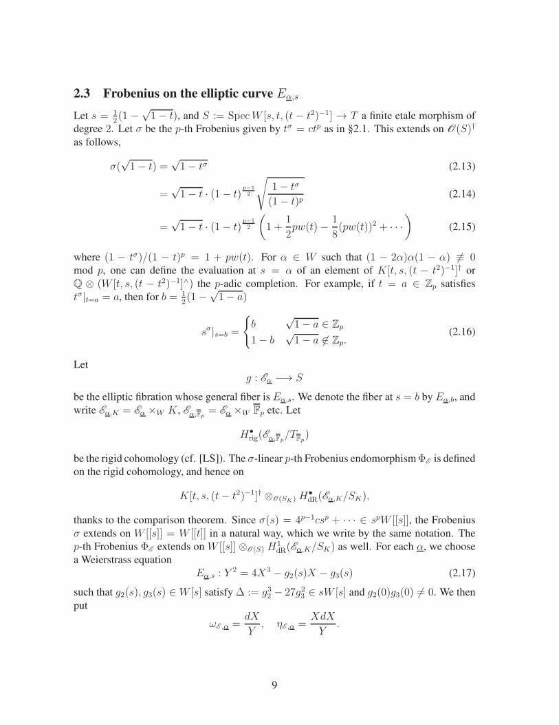
2.3 Frobenius on the elliptic curve Eα,s

Let s = 12(1 −

√1− t), and S := SpecW [s, t, (t − t2)−1] → T a finite etale morphism of

degree 2. Let σ be the p-th Frobenius given by tσ = ctp as in §2.1. This extends on O(S)†

as follows,

σ(√1− t) =

√1− tσ (2.13)

=√1− t · (1− t)

p−12

√1− tσ

(1− t)p(2.14)

=√1− t · (1− t)

p−12

(1 +

1

2pw(t)− 1

8(pw(t))2 + · · ·

)(2.15)

where (1 − tσ)/(1 − t)p = 1 + pw(t). For α ∈ W such that (1 − 2α)α(1 − α) 6≡ 0mod p, one can define the evaluation at s = α of an element of K[t, s, (t − t2)−1]† or

Q ⊗ (W [t, s, (t − t2)−1]∧) the p-adic completion. For example, if t = a ∈ Zp satisfies

tσ|t=a = a, then for b = 12(1−

√1− a)

sσ|s=b =

{b

√1− a ∈ Zp

1− b√1− a 6∈ Zp.

(2.16)

Let

g : Eα −→ S

be the elliptic fibration whose general fiber is Eα,s. We denote the fiber at s = b by Eα,b, and

write Eα,K = Eα ×W K, Eα,Fp= Eα ×W Fp etc. Let

H•rig(Eα,Fp

/TFp)

be the rigid cohomology (cf. [LS]). The σ-linear p-th Frobenius endomorphismΦE is defined

on the rigid cohomology, and hence on

K[t, s, (t− t2)−1]† ⊗O(SK) H•dR(Eα,K/SK),

thanks to the comparison theorem. Since σ(s) = 4p−1csp + · · · ∈ spW [[s]], the Frobenius

σ extends on W [[s]] = W [[t]] in a natural way, which we write by the same notation. The

p-th Frobenius ΦE extends on W [[s]] ⊗O(S) H1dR(Eα,K/SK) as well. For each α, we choose

a Weierstrass equation

Eα,s : Y2 = 4X3 − g2(s)X − g3(s) (2.17)

such that g2(s), g3(s) ∈ W [s] satisfy ∆ := g32 − 27g23 ∈ sW [s] and g2(0)g3(0) 6= 0. We then

put

ωE ,α =dX

Y, ηE ,α =

XdX

Y.

9

Lemma 2.5 Let Ds = s dds

and put E := 2g2Dsg3 − 3Dsg2 · g3. Then

DsωE ,α = −Ds∆

12∆ωE ,α +

3E

2∆ηE ,α,

DsηE ,α = −g2E

8∆ωE ,α +

Ds∆

12∆ηE ,α.

Proof. This is well-known, e.g. [A-C, Theorem 7.1]. �

Lemma 2.6 Let DS = K[s, t, ddt] be the Wyle algebra of S. Let Ds := s d

ds. Then for

α = (α0, α1,12), we have isomorphisms

DS/DSPα0α1

∼=−→ H1dR(Eα,K/SK), 1DS

7−→ ωE ,α, (2.18)

O(SK)⊗O(T ) Vα = DS · ωα

∼=−→ Sym2H1dR(Eα,K/SK), ωα 7−→ ω2

E ,α (2.19)

of left DS-modules, see (2.1) for the definition of Pα0α1 and (2.2) for Vα.

Proof. We may replace K with C. It is a standard exercise to show that there is a homology

cycle γ ∈ H1(Eα,s,Q) that is a vanishing cycle at s = 0, such that

∫

γ

ωE ,α = 2πi 2F1

(α0, α1

1; s). (2.20)

This implies DSωE ,α ( H1dR(Eα,K/SK), and hence DSωE ,α = 0 as H1

dR(Eα,K/SK) is ir-

reducible. This shows that the arrow (2.18) is well-defined. Since both side of (2.18) are

irreducible, it turns out to be bijective.

Next we show (2.19). Employing Clausen’s formula (1.10) together with the transforma-

tion formula [NIST, 15.8.18], we have

3F2

(α0, α1,

12

1, 1; t

)= 2F1

(α0, α1

1; s)2

, s =1

2(1−

√1− t). (2.21)

Therefore we have ∫

γ⊗γ

Pα(ω2E ,α) = 0

and hence that the map

O(S)⊗O(T ) Vα∼= DS/DSPα −→ Sym2H1

dR(Eα,K/SK), A 7−→ A(ω2E ,α)

is well-defined. Since both sides are irreducible, this is bijective. �

10

Let us describe the Frobenius ΦE . Let W ((t))∧ be the p-adic completion of W ((t)) =W [[t]][t−1]. Let α = (α0, α1,

12). According to [A-M, §5.1], there is a basis (de Rham

symplectic basis)

ωα,E , ηα,E ∈ W ((t))∧ ⊗O(S) H1dR(Eα,K/SK)

which satisfies (cf. [A-C, Propositions 4.1, 4.2])

(Ds(ωE ,α) Ds(ηE ,α)

)=(ωE ,α ηE ,α

)( 0 0Dsqq

0

)(2.22)

where q ∈ W [[s]] is defined by j(Eα,s) = 1/q + 744 + 196884q + · · · , and

(ΦE (ωE ,α) ΦE (ηE ,α)

)=(ωE ,α ηE ,α

)( p 0−pτ (σ)(s) 1

)(2.23)

where τ (σ)(s) ∈ W [[s]] is the power series given in [A-C, Proposition 4.2]. The explicit

relation with the basis {ωE ,α, ηE ,α} is

ωE ,α =κ

Fα0,α1(s)ωE ,α, ηE ,α = −H(s)ωE ,α + κ−1Fα0,α1(s)ηE ,α, κ :=

√− g2(0)

18g3(0)(2.24)

where H(s) is the power series given in [A-C, Propositions 7.3].

We pick up the results which shall be necessary in our proof of Theorem 2.4.

Proposition 2.7 Let

(ΦE (ωE ,α) ΦE (ηE ,α)

)=(ωE ,α ηE ,α

)(pA0 B0

pA1 B1

). (2.25)

Then all of A0, . . . , B1 belong to W [s, t,√1− t]† and they satisfy

A0B1 −A1B0 = 1 (2.26)

and

B1 ≡ ǫFα0α1(s)

Fα0α1(sσ)

mod p, ǫ := F (κ)/κ = ±1. (2.27)

Proof. See [A-C, Propositions 4.3]. Note that (2.26) and (2.27) directly follow from the

explicit descriptions of A0, . . . , B1 in loc.cit. �

2.4 Comparison Theorem

Theorem 2.8 Under the isomorphism

O(SK)† ⊗O(TK ) Vα

∼= O(SK)† ⊗O(SK ) Sym

2H1dR(Eα,K/SK), (2.28)

induced from (2.19), the Frobenius Φ on the left agrees with Sym2ΦE on the right.

11

Proof. It follows from the main theorem of [Dw2] that they agree up to a constant c, namely

Φ = c Sym2ΦE . We show c = 1. To do this we employ the basis {ωE ,α, ηE ,α}. Since

〈ξα, ηα〉 = 〈Dωα, D2ωα〉 ⊂ W ((t))∧ ⊗O(T ) Vα

by (2.6), one finds that under the isomorphism (2.28), this corresponds to the subspace

〈D(ω2E ,α), D

2(ω2E ,α)〉 = 〈ωE ,αηE ,α, η

2E ,α〉 ⊂ W ((t))∧ ⊗O(S) Sym

2H1dR(Eα,K/SK)

where the above equality follows from (2.22). Hence the isomorphism (2.28) induces an

isomorphism

(W ((t))∧ ⊗O(T ) Vα)/〈ξα, ηα〉∼=

// (W ((t))∧ ⊗O(S) Sym2H1

dR(Eα,K/SK))/〈ωE ,αηE ,α, η2E ,α〉

W ((t))∧ ωα W ((t))∧ ω2E ,α

compatible with respect to Φ and c Sym2ΦE . It sends ωα to κ2ω2E ,α by (2.3) and (2.24)

together with (2.21). Since

Φ(ωα) ≡ p2ωα mod 〈ξα, ηα〉 by (2.8)

Sym2ΦE (ω2E ,α) ≡ p2ω2

E ,α mod 〈ωE ,αηE ,α, η2E ,α〉 by (2.23)

one has

c =F (κ2)

κ2= 1

as required. �

Corollary 2.9 Let Frob(σ)α be the matrix defined in Definition 2.2, and let A0, . . . , B1 be as

in (2.25). Let X be the 3× 3 matrix defined by

(ωα Dωα D2ωα

)=(ω2

E ,α ωE ,αηE ,α η2E ,α

)X

under the identification (2.28). Then

Frob(σ)α = X−1

p2A20 pA0B0 B2

0

2p2A0A1 p(A0B1 + A1B0) 2B0B1

p2A21 pA1B1 B2

1

Xσ

Proof. Immediate from Theorem 2.8. �

12

2.5 Proof of Theorem 2.4

Lemma 2.10 Let q = pm, and let φq = (φp)m ∈ GFp

be the q-th Frobenius. Let a ∈ W (Fq)satisfy that a(1−a) 6≡ 0 mod p. Put b = 1

2(1−

√1− a). Let σa be given by tσa = F (a)a−ptp

where F is the p-th Frobenius on W (Fq). Then

det(I − (Frob(σa)α )2m|t=aT ) = det(1− (φ2

q)−1T | Sym2H1

et(Eα,b,Fp,Ql)) (2.29)

where GFq2

acts on H•et(Eα,b,Fp

,Ql) as the reduction of Eα,b is defined over Fq2 . If√1− a ∈

W (Fq), then

det(I − (Frob(σa)α )m|t=aT ) = det(1− (φq)

−1T | Sym2H1et(Eα,b,Fp

,Ql)) (2.30)

where GFqacts on H•

et(Eα,b,Fp,Ql) as the reduction of Eα,b is defined over Fq.

Proof. Let K0 be the fractional field of W (Fq), and we denote by V †α,K0

the module (2.7)

replacing K with K0. Then Φ|t=a acts on V †α,K0

|t=a as a F -linear map, and the m-fold com-

position Φm|t=a is a K0-linear map providing the characteristic polynomial of (Frob(σa)α )m.

On the other hand, Φ2E|s=b acts on H1

dR(Eα,b/K0) as a F -linear map, and the K0-linear map

Φ2mE

|s=b provides the right hand side of (2.29). If√1− a ∈ W (Fq), then ΦE |s=b acts on

H1dR(Eα,b/K0), and Φm

E|s=b provides the right hand side of (2.30). Therefore the lemma

follows by Theorem 2.8. �

Lemma 2.11 Let a ∈ Zp satisfy that a(1− a) 6≡ 0 mod p, and b := 12(1−

√1− a). Then

det Frob(σ)α |s=b =

(1− a

p

)p3. (2.31)

Let A0, . . . , B1 be as in (2.25). If√1− a 6∈ Zp, then

TrFrob(σa)α |t=a =

(pA0 − B1)2|s=b + p α = (1

2, 12, 12), (1

6, 56, 12)

(p(A0 + 2A1)−B1)2|s=b + p α = (1

3, 23, 12)

(p(A0 − 13A1)−B1)

2|s=b + p α = (14, 34, 12).

(2.32)

Proof. One has det Frob(σ)α = p3(1− 2s)3/(1− 2sσ)3 by (2.26) and Corollary 2.9. So (2.31)

is immediate by (2.16). To show (2.32), we need an explicit computation of the matrix X .

For example, in case α = (12, 12, 12), one has

X =

1 −1

37s2−7s+118(2s−1)2

0 12s−1

−10s2+10s−13(2s−1)3

0 0 12(2s−1)2

by Lemma 2.5, and then (2.32) follows. For other α’s, the proof is similar (left to the reader).

�

13

Proof of Theorem 2.4. We want to compute the characteristic polynomial

det(I − Frob(σa)α |t=aT ) = (1− γ1T )(1− γ2T )(1− γ3T ) ∈ Z[T ].

If√1− a ∈ Zp, then Theorem 2.4 is immediate from (2.30). We suppose

√1− a 6∈ Zp until

the end of the proof. We have

γ1γ2γ3 = −p3 (2.33)

by (2.31). Let

det(1− φ−1p2 T | H1

et(Eα,b,Fp,Ql)) = (1− αp2(Eα,b)T )(1− βp2(Eα,b)T ) ∈ Z[T ]

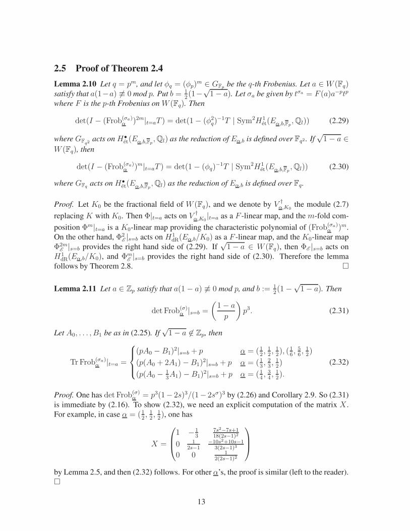
be the characteristic polynomial for the p2-th Frobenius φp2 ∈ GFp2

. We know from (2.29)

that the triplet (γ21 , γ

22 , γ

23) agrees with (p2, αp2(Eα,b)

2, βp2(Eα,b)2) up to permutation. We

may let

γ1 = ±p, γ2 = εαp2(Eb), γ3 = ε′βp2(Eα,b) (2.34)

where ε, ε′ = ±1.

If Eα,b has a supersingular reduction at p, then ordp(αp2(Eα,b)) > 0 and ordp(βp2(Eb)) >0, and hence ordp(γi) > 0 for every i. By (2.32), there is e ∈ W such that

γ1 + γ2 + γ3 = e2 + p

which is zero modulo p, whence

γ1 + γ2 + γ3 ≡ p mod p2. (2.35)

Suppose γ1 = p. Then γ2 + γ3 ≡ 0 mod p2 by (2.35) and γ2γ3 = −p2 by (2.33). Since

γ2 + γ3 is a rational integer satisfying |γ2 + γ3| ≤ 2p, it turns out that γ2 + γ3 = 0 and

hence (γ2, γ3) = (p,−p) or (−p, p). Suppose γ1 = −p. Then γ2 + γ3 ≡ 2p mod p2 and

γ2γ3 = p2. Since |2p+np2| ≤ 2p⇔ n = 0 as p ≥ 5, one concludes γ2+ γ3 = 2p and hence

γ2 = γ3 = p. In both cases the triplet (γ1, γ2, γ3) agrees with (p, p,−p) up to permutation.

This completes the proof of Theorem 2.4 when Eα,b has a supersingular reduction.

The rest is the case that Eb has an ordinary reduction. We may let ordp(αp2(Eα,b)) = 0and ordp(βp2(Eα,b)) > 0. We first see that ε = ε′ in (2.34). Indeed, if ε 6= ε′, then

αp2(Eα,b)−βp2(Eα,b) is a rational integer as γ1+γ2+γ3 ∈ Z. Since αp2(Eα,b)+βp2(Eα,b) ∈Z, it turns out that αp2(Eα,b) is a rational integer satisfying |αp2(Eb)| = p, and hence

αp2(Eα,b) = ±p. This contradicts with the assumption ordp(αp2(Eα,b)) = 0. We thus

have ε = ε′. We want to show

ε =

(dαp

), (2.36)

which finishes the proof of Theorem 2.4 by (2.33). We denote f(s)<n =∑

i<n aisi the

truncated polynomial for a series f(s) =∑∞

i=0 aisi. It follows from (2.27) and (2.32) that

we have

εαp2(Eα,b) ≡(

Fα0α1(s)

Fα0α1(sσ)

)2 ∣∣∣∣s=b

≡ (Fα0α1(s)<p)2|s=b mod p

14

where the second congruence follows from the Dwork congruence ([Dw1, Theorem 3]). On

the other hand, Dwork’s unit root formula ([VdP, (7.14)]) yields

αp2(Eα,b) =Fα0α1(s)

Fα0α1(sσ2)

∣∣∣∣s=b

=Fα0α1(s)

Fα0α1(sσ)

Fα0α1(sσ)

Fα0α1(sσ2)

∣∣∣∣s=b

(2.16)=

Fα0α1(s)

Fα0α1(sσ)

∣∣∣∣s=b

· Fα0α1(s)

Fα0α1(sσ)

∣∣∣∣s=1−b

≡ Fα0α1(s)<p|s=b · Fα0α1(s)<p|s=1−b mod p

Therefore we have

ε ≡ Fα0α1(s)<p|s=b · (Fα0α1(s)<p|s=1−b)−1 mod p.

We compute the right hand side. To do this, we see the Cartier operator C for the reductions

of Eα,b and Eα,1−b respectively. Let α = (12, 12, 12). Recall that the elliptic curve Eα,s is

defined by the Weierstrass equation y2 = x(x− 1)(x− s). Then one has

C

(dx

y

)= (−1)

p−12 (F 1

2, 12(s)<p|s=b)

dx

y, C

(dx

y

)= (−1)

p−12 (F 1

2, 12(s)<p|s=1−b)

dx

y

for Eα,b and Eα,1−b respectively. Using an isomorphism

E 12, 12, 12,b : y

2 = x(x− 1)(x− b) −→ E ′12, 12, 12,1−b

: −y2 = x(x− 1)(x− 1 + b) (2.37)

(x, y) 7−→ (1− x, y),

it follows

ε ≡F 1

2, 12(s)<p|s=b

F 12, 12(s)<p|s=1−b

≡ (√−1)p/

√−1 =

(−1

p

)mod p.

This completes the proof of (2.36) in case α = (12, 12, 12). The proof in the other cases goes

in the same way with use of the isogeny

E 13, 23, 12,b : y

2 = y2 = x3 + (3x+ 4b)2 −→ E ′13, 23, 12,1−b

: −3y2 = y2 = x3 + (3x+ 4− 4b)2

(2.38)

(x, y) 7−→(x3 + 12x2 + 48bx+ 64b2

−3x2,x3 − 48bx− 128b2

9x3y

),

E 14, 34, 12,b : y

2 = x(x2 − 2x+ 1− b) −→ E ′14, 34, 12,1−b

: −2y2 = x(x2 − 2x+ b) (2.39)

(x, y) 7−→(−1

2x+ 1 +

b− 1

2x,y(x2 + b− 1)

4x2

)

E 16, 56, 12,b : y

2 = 4x3 − 3x+ 1− 2b −→ E ′16, 56, 12,1−b

: −y2 = 4x3 − 3x− 1 + 2b (2.40)

(x, y) 7−→ (−x, y).

This completes the proof of Theorem 2.4.

15

2.6 Cases α = (12,12,

12), (

16,

56,

12)

Theorem 2.12 Let α be either of (12, 12, 12), (1

6, 56, 12). Let Cα,t be the elliptic curves in (1.8).

Then

det(I − Frob(σa)α |t=a) =

(1−

(1− a

p

)pT

)(1−

(1− a

p

)ap2(Cα,a)T + p2T 2

)

for any a ∈ Zp such that a(1− a) 6≡ 0 mod p.

Proof. The proof goes in a similar way to that of Theorem 2.4 and it is simpler. We sketch

the outline. The details are left to the reader.

The key formula on the hypergeometric function is

3F2

(α0, α1,

12

1, 1; t

)= 2F1

( 12α0,

12α1

1; t

)2

(Clausen)

= (1− t)−α02F1

(12α0, 1− 1

2α1

1;

t

t− 1

)2

([NIST, 15.8.1]).

Let α = (12, 12, 12). Then

3F2

(12, 12, 12

1, 1; t

)= (1− t)−

12 2F1

(14, 34

1;

t

t− 1

)2

.

Since the “2F1” in the right is the period of the elliptic curve Cα,t, one can show an isomor-

phism

Vα∼= Sym2H1

dR(Cα,t/T )⊗ O(T )√1− t

of F -isocrystals in a similar way to the proof of Lemma 2.6, where O(T )√1− t denotes

the minus part H0dR(S/T )

− with respect to the involution in Aut(S/T ) ∼= Z/2Z. The rest is

automatic.

Let α = (16, 56, 12). Then

3F2

(16, 56, 12

1, 1; t

)= 2F1

(112, 512

1; t

)2

and the period of Cα,t is

(1− t)−14 2F1

(112, 512

1; t

).

Therefore one can show

Vα∼= Sym2H1

dR(Cα,t/T )⊗ O(T )√1− t

as well.

�

16

3 Galois representations of K3 surfaces of Hypergeometric

type

3.1 Lemmas on Galois representations of Kummer surfaces

For an abelian surface A over a field F of characteristic 0, the minimal resolution of the quo-

tient A/〈−1〉 is a K3 surface, which we write by Km(A) and call the Kummer K3 surface.

Then one finds that there is a natural bijection

H2et,tr(Km(A),Ql)

∼=−→ H2et,tr(A,Ql)

on the transcendental part H2et,tr(X,Ql) := H2

et(X,Ql)/NS(X)⊗Ql of the l-adic cohomol-

ogy.

Lemma 3.1 Suppose that F is a number field.

(1) The GF -representation H2et(Km(A),Ql) is semisimple.

(2) Let VQl⊂ H2

et(Km(A),Ql) and V ′Ql

⊂ H2et(Km(A′),Ql) be sub GF -representations.

Suppose that there is a set S of primes of F with density 1 such that

Tr(φ℘ | VQl) = Tr(φ℘ | V ′

Ql) (3.1)

for every ℘ ∈ S where φ℘ is the Frobenius at ℘. Then there is an isomorphism VQl∼=

V ′Ql

of GF -representations.

Proof. (1) follows from a theorem of Faltings which asserts that H1et(A,Ql) is semisimple.

(2) follows from the fact that VQland V ′

Qlare semisimple (cf. [Se, I, 2.3]). �

Lemma 3.2 Let X be a K3 surface over a number field F such that ρ(X) ≥ 19. Then Xis singular (i.e. ρ(X) = 20) if and only if dimQl

H2et(X,Ql(1))

GF ′ = 20 for some finite

extension F ′/F .

If we admit the Tate conjecture for cycles on X ×X of codimension 2, then we can drop the

condition “ρ(X) ≥ 19”.

Proof. By the assumption, X has the Shioda-Inose structure, namely there is an elliptic curve

E over a number field such that the Kummer surface Km(E × E) is isogenous to X. Then

X is singular if and only if E has a CM. The isogeny induces a surjective map

Sym2H1et(E,Ql) −→ H2

et(X,Ql)/NS(X)⊗Ql

of GL-representations for some finite extensionL/F . Suppose that dimQlH2

et(X,Ql(1))GF ′ =

20 for some F ′/F . We may assume L ⊂ F ′. We want to show ρ(X) = 20. Suppose

that ρ(X) = 19. Then since the above map is bijective, the fixed part (Sym2H1et(E,Ql) ⊗

Ql(1))GF ′ is 1-dimensional. This is equivalent to that dimQl

End(H1et(E,Ql))

GF ′ = 2. Since

End(E)⊗Ql∼= End(H1

et(E,Ql))GF ′ by a theorem of Faltings, this implies that E has a CM

and hence that X is singular. This is a contradiction. This completes the proof of the “if”

part. The “only if” part is obvious. �

17

3.2 K3 surfaces of Hypergeometric type

Let

f : X −→ T = SpecQ[t, (t− t2)−1]

be a projective smooth family of K3 surfaces. Let D = Q[t, (t − t2)−1, ddt] be the Wyle

algebra of T . Put X t := X ×T Q(t) and set

VdR(X /T ) = Coim[H2dR(X /T ) → H2

dR(X t)/NS(X t)⊗Q(t)]

a D-module which is free of finite rank over O(T ).

Definition 3.3 We call f of hypergeometric type Fα(t) if the following conditions hold.

(i) ρ(X t) = 19 or equivalently VdR(X /T ) is of rank 3 over O(T ).

(ii) There is an isomorphism VdR(X /T ) ∼= D/DPα of left D-modules, where Pα is the

hypergeometric differential operator (2.1).

Let α be either of the following as before,

(1

2,1

2,1

2

),

(1

3,2

3,1

2

),

(1

4,3

4,1

2

),

(1

6,5

6,1

2

).

Let p > 3 be a prime and put W = W (Fp) and K = FracW . Suppose that there is an

integral regular flat model

fZ(p): XZ(p)

−→ TZ(p)

over the ring Z(p) ⊂ Q such that fZ(p)is smooth projective. For a ∈ Z(p) such that a(1 −

a) 6≡ 0 mod p, we denote by Xa the fiber at t = a. We denote XW = XZ(p)×Z(p)

W ,

XK = XW ×W K, . . . as before. Recall from Definition 2.2 the F -isocrystal

V crys(α, σ) =(Vα, V

†α ,∇,Φ, σ

).

Thanks to the comparison

K[t, (t− t2)−1]† ⊗O(TK ) H2dR(X /T ) ∼= H2

rig(XFp/TFp

)

of the de Rham and rigid cohomology, the p-th Frobenius on

K[t, (t− t2)−1]† ⊗O(TK ) VdR(XK/TK)

is defined, which we denote by ΦX . We fix an isomorphism VdR(X /T ) ∼= D/DPα (this

is unique up to scalar as both sides are irreducible). It follows from [Dw2] that there is a

constant εp such that

Φ = εpΦX .

18

Let a ∈ Z(p) such that a(1 − a) 6≡ 0 mod p and let σ = σa given by σa(t) = a1−ptp. By

Theorem 2.4, the characteristic polynomial of ΦX |t=a on VdR(Xa/Qp) is

(1−

(1− a

p

)pεpT

)(1− εpAa,pT + (εppT )

2).

Since this is a polynomial with coefficients in Z and p± Aa,p 6= 0, it turns out that εp ∈ Q×

(not depend on a). Moreover since (det VdR(Xa/Qp))⊗2 is isomorphic to the Tate object

Qp(−6), one has ε6p = 1 and hence εp = ±1. Using the l-adic cohomology,

Vet(Xa)Ql:= Coim[H2

et(Xa,Ql) → H2et(X t,Ql)/NS(X t)⊗Ql], Xa := Xa ×Z(p)

Q,

one has

det(φ−1p | (det Vet(Xa)Ql

)⊗Ql(3)) = ε3p

(1− a

p

)= εp

(1− a

p

).

Define a quadratic character χX /T by

χX /T : GQ −→ Aut((detVet(Xa)Ql)⊗Ql(3)⊗ χ1−a) ∼= Q×

l (3.2)

where χ1−a denotes the quadratic character for Q(√1− a). This does not depend on either

a or l, takes value in {±1} and satisfies χX /T (φp) = εp for almost all p.

Summing up the above, we have

Theorem 3.4 Let the notation and assumption be as above. Then

det(1−φ−1p T | Vet(Xa)Ql

) =

(1−

(1− a

p

)χX /T (φp)pT

)(1−χX /T (φp)Aa,pT +p2T 2).

Theorem 3.5 Let F be a number field. Let a ∈ F \ {0, 1} be arbitrary. Then there is an

isomorphism

Vet(Xa)Ql∼= Sym2H1

et(Eα,b,Ql)⊗ χX /T

of GF (√1−a)-representations where Eα,b is the elliptic curve in Theorem 2.4.

Proof. By virtue of Lemma 3.1 (2), it is enough to show that

Tr(φ℘ | Vet(Xa)Ql) = Tr(φ℘ | Sym2H1

et(Eα,b,Ql)⊗ χX /T ).

for almost all primes ℘ of F (√1− a). However this follows from Lemma 2.10 (2.30). �

In the case α = (12, 12, 12) or (1

6, 56, 12), the same discussion replacing Theorem 2.4 with

Theorem 2.12 yields the following.

Theorem 3.6 Let α be either of (12, 12, 12) or (1

6, 56, 12). Then, for a ∈ F \ {0, 1}, there is an

isomorphism

Vet(Xa)Ql∼= Sym2H1

et(Cα,a,Ql)⊗ χX /T ⊗ χ1−a

of GF -representations where Cα,a is the elliptic curve in Theorem 2.12.

19

Theorem 3.7 Let a ∈ Q \ {0, 1}. Then Xa is singular (i.e. the Picard number 20) if and

only if Eα,b has a CM.

Proof. Immediate from Theorem 3.5 and Lemma 3.2. �

It is known that there are 13 rational CM j-invariants, and 58 CM j-invariants that are

quadratic numbers but not rational ([D-LR]). The complete list of them is available by

SAGE. We thus have the complete list of rational a’s such that Xa is singular.

a ∈ Q \ {0, 1} such that Xa is singular

α =

(1

2,1

2,1

2

)−1, 4,

1

4,−8,−1

8, 64,

1

64

α =

(1

3,2

3,1

2

)−4,

1

2,−1

24,−1

210,−32

24,33

24,2

33,33

2,−1

245,4

53,−1

2456,

−1

23337

α =

(1

4,3

4,1

2

) −1

22,1

32,1

34,−1

243,−24

32,−1

2234,25

34,28

34,

−1

26345,1

74,

−1

223474,−28

3472,

1

34112,

1

38114

α =

(1

6,5

6,1

2

) −1

29,−33

29,22

53,−26

53,

−1

21253,−32

2953,33

53,23

113,

−1

2953113,

26

53173,

−1

21253233293

Remark 3.8 It is natural to expect that the Shioda-Inose structure ofXa is given by Km(Eα,b×Eα,b), the author does not have a proof though.

Remark 3.9 For the K3 families (i), . . . , (iv) in §1, the character χX /T is trivial. For exam-

ple, let X → T be the family (iii). There is an isomorphism ([As1, Corollary 3.6])

D/DPα

∼=−→ VdR(X /T ), A 7−→ Aω1,1,1

where ωi,j,k is the regular 2-form defined in [As1, (2.7)]. Letting ω := ω1,1,1, we construct a

basis {ω, ξ, η} in the same as in §2.1. Then it is shown that

ΦX (ω) ≡ p2ω mod 〈ξ, η〉

in the proof of [As2, Theorem 4.5]. This shows εp = 1, namely χX /T is trivial. For the other

K3 families, one can show that χX /T is trivial in the same way (the argument in the proof of

[As2, Theorem 4.5] works).

20

References

[AOP] Ahlgren, S.; Ono, K.; Penniston, D., Zeta Functions of an infinite family of K3

surfaces. American Journal of Mathematics, Vol. 124, No. 2 (Apr., 2002), pp.

353–368.

[As1] Asakura, M., A generalization of the Ross symbols in higher K-groups and hyper-

geometric functions I, arXiv.2003.10652

[As2] , A generalization of the Ross symbols in higher K-groups and hypergeo-

metric functions II, arXiv:2102.07946.

[A-C] Asakura, M. and Chida, M., A numerical approach toward the p-adic Beilinson

conjecture for elliptic curves over Q. arXiv:2003.08888

[A-M] Asakura, M. and Miyatani, K., Milnor K-theory, F -isocrystals and syntomic reg-

ulators. arXiv:2007.14255.

[D-LR] Daniels, H-B., Lozano-Robledo, A., On the number of isomorphism classes of CM

elliptic curves defined over a number field. J. Number Theory 157 (2015), 367–

396.

[Dw1] Dwork, B., p-adic cycles. Publ. Math. IHES, tome 37 (1969), 27–115.

[Dw2] , On the uniqueness of Frobenius operator on differential equations. in

Algebraic Number Theory - in Honor of K. Iwasawa, Advanced Studies in Pure

Math. 17, Academic Press, Boston, 1989, 89–96.

[E-S] Elkies, N. and Schutt, M., K3 families of higher Picard rank. preprint.

[vG-T] van Geemen, B., Top, J., An isogeny of K3 surfaces. Bull. London Math. Soc. 38

(2006), no. 2, 209–223.

[Go1] Goodson, H., Hypergeometric functions and relations to Dwork hypersurfaces.

Int. J. Number Theory, Volume 3 (2), 2017, 439–485.

[Go2] , A complete hypergeometric point count formula for Dwork hypersur-

faces. J. Number Theory, Volume 179, 2017, 142–171.

[Ka] Katz, N., Another look at the Dwork family, Algebra, arithmetic, and geometry: in

honor of Yu. I. Manin. Vol. II, 89–126, Progr. Math., 270, Birkhauser, 2009.

[Ko] Koblitz, N., The number of points on certain families of hypersurfaces over finite

fields. Compositio Math., tome 48, 1983, 3–23.

[Mc] McCarthy, D., The number of Fq-points on Dwork hypersurfaces and hypergeo-

metric functions. Res. Math. Sci., Volume 4 (4), 2017, 1–15.

21

[Mi] K. Miyatani, K., Monomial deformations of certain hypersurfaces and two hyper-

geometric functions. Int. J. Number Theory, Volume 11 (8), 2015, 2405–2430.

[Mo] Morrison, D. R., On K3 surfaces with large Picard number, Invent. Math. 75,

(1984), 105–121.

[Na] Naskrecki, B., On a certain hypergeometric motive of weight 2 and rank 3.

arXiv:1702.07738

[O] Otsubo, N., Hypergeometric functions over finite fields. arXiv:2108.06754.

[VdP] Van der Put, M., The cohomology of Monsky and Washnitzer. Introductions aux

cohomologies p-adiques (Luminy, 1984). Mem. Soc. Math. France (N.S.) No. 23

(1986), 33–59.

[Se] Serre, J-P., Abelian l-adic representations and elliptic curves. Benjamin, 1968.

[LS] Le Stum, B., Rigid cohomology. Cambridge Tracts in Mathematics, 172. Cam-

bridge University Press, Cambridge, 2007. xvi+319 pp.

[NIST] NIST Handbook of Mathematical Functions. Edited by Frank W. J. Olver, Daniel

W. Lozier, Ronald F. Boisvert and Charles W. Clark. Cambridge Univ. Press, 2010.

22