25
Zhen Tian Jeff Lee Visut Hemithi Huan Zhang Diana Aguilar Yuli Yan A Deep Analysis of A Random Walk
| Date post: | 30-Dec-2015 |
| Category: |
Documents |
| Upload: | paul-duncan |
| View: | 44 times |
| Download: | 0 times |

Zhen Tian
Jeff Lee
Visut Hemithi
Huan Zhang
Diana Aguilar
Yuli Yan
A Deep Analysis of A Random WalkA Deep Analysis of A Random Walk

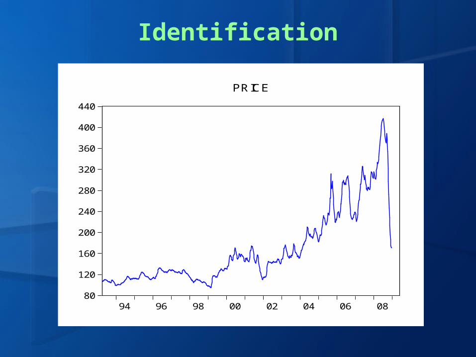
Identification
80
120
160
200
240
280
320
360
400
440
94 96 98 00 02 04 06 08
PRICE
0
20
40
60
80
100
120
140
120 160 200 240 280 320 360 400
Series: PRICESample 4/05/1993 5/25/2009Observations 821
Mean 169.6928Median 144.0000Maximum 416.5000Minimum 94.90000Std. Dev. 72.61291Skewness 1.377958Kurtosis 4.121595
Jarque-Bera 302.8479Probability 0.000000
Identification
80
120
160
200
240
280
320
360
400
440
94 96 98 00 02 04 06 08
PRICE
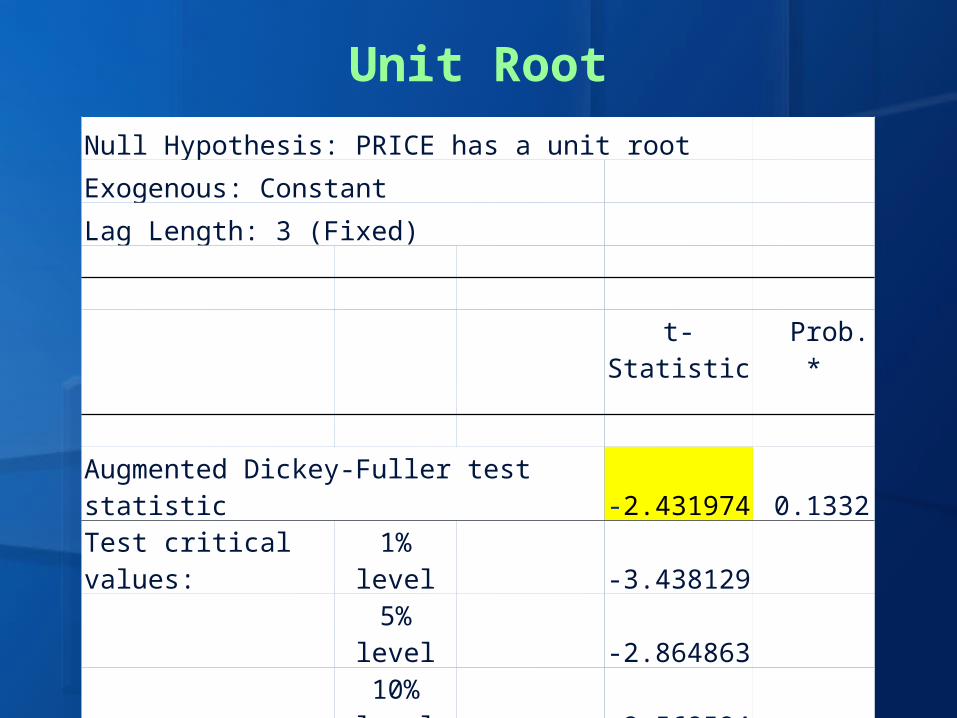
Unit Root
Null Hypothesis: PRICE has a unit root
Exogenous: Constant
Lag Length: 3 (Fixed)
t-Statistic Prob.*
Augmented Dickey-Fuller test statistic -2.431974 0.1332
Test critical values: 1% level -3.438129
5% level -2.864863
10% level -2.568594

Pre-Whitening
-.15
-.10
-.05
.00
.05
.10
.15
.20
94 96 98 00 02 04 06 08
DLNPRICE
Log Transformation
Trend in Var.
Difference
Trend in Mean

Pre-Whitening
0
40
80
120
160
200
240
280
-0.10 -0.05 -0.00 0.05 0.10 0.15
Series: DLNPRICESample 4/05/1993 5/25/2009Observations 820
Mean 0.000574Median -0.000909Maximum 0.161180Minimum -0.098922Std. Dev. 0.019665Skewness 0.259126Kurtosis 11.59559
Jarque-Bera 2533.555Probability 0.000000

Unit Root
Null Hypothesis: DLNPRICE has a unit root
Exogenous: Constant
Lag Length: 4 (Fixed)
t-Statistic Prob.*
Augmented Dickey-Fuller test statistic -9.819079 0.0000
Test critical values: 1% level -3.438149
5% level -2.864872
10% level -2.568599

Dependent Variable: DLNPRICEMethod: Least SquaresSample (adjusted): 5/17/1993 12/22/2008Included observations: 815 after adjustmentsConvergence achieved after 6 iterationsBackcast: 1/11/1993 5/10/1993
Variable Coefficient Std. Error t-Statistic Prob.
C 0.000421 0.001769 0.238003 0.8119AR(1) 0.503803 0.034771 14.48920 0.0000AR(2) 0.104044 0.039420 2.639331 0.0085AR(3) 0.143444 0.036466 3.933679 0.0001AR(5) -0.124364 0.032993 -3.769439 0.0002MA(8) 0.103332 0.037023 2.791007 0.0054
MA(18) 0.118155 0.036499 3.237194 0.0013
R-squared 0.389743 Mean dependent var 0.000545Adjusted R-squared 0.385211 S.D. dependent var 0.019718S.E. of regression 0.015461 Akaike info criterion -5.492468Sum squared resid 0.193141 Schwarz criterion -5.452073Log likelihood 2245.181 F-statistic 86.00538Durbin-Watson stat 2.000720 Prob(F-statistic) 0.000000
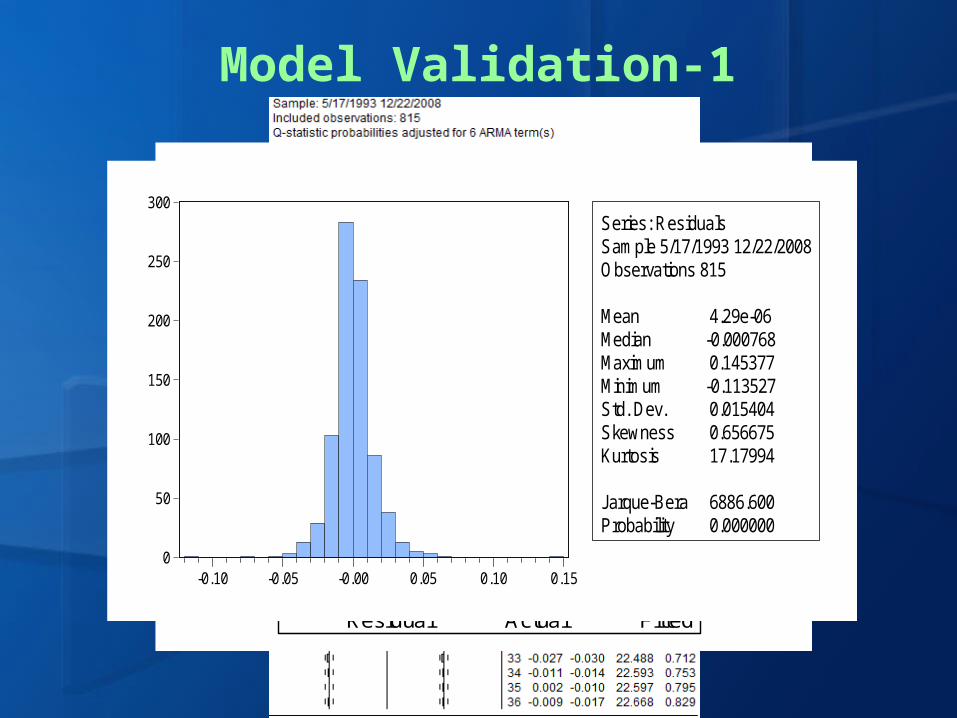
Model Validation-1
-.12
-.08
-.04
.00
.04
.08
.12
.16
-.2
-.1
.0
.1
.2
1994 1996 1998 2000 2002 2004 2006 2008
Residual Actual Fitted
0
50
100
150
200
250
300
-0.10 -0.05 -0.00 0.05 0.10 0.15
Series: ResidualsSample 5/17/1993 12/22/2008Observations 815
Mean 4.29e-06Median -0.000768Maximum 0.145377Minimum -0.113527Std. Dev. 0.015404Skewness 0.656675Kurtosis 17.17994
Jarque-Bera 6886.600Probability 0.000000

Model Validation-2
Breusch-Godfrey Serial Correlation LM Test:
F-statistic 0.105569 Prob. F(2,806) 0.899825
Obs*R-squared 0.213376 Prob. Chi-Square(2) 0.898806.000
.004
.008
.012
.016
.020
.024
1994 1996 1998 2000 2002 2004 2006 2008
RESIDSQ


Model Validation-ARCH GARCH (1)
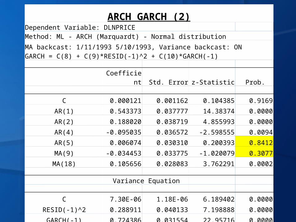
ARCH GARCH (2)Dependent Variable: DLNPRICEMethod: ML - ARCH (Marquardt) - Normal distribution
MA backcast: 1/11/1993 5/10/1993, Variance backcast: ONGARCH = C(8) + C(9)*RESID(-1)^2 + C(10)*GARCH(-1)
Coefficient Std. Error z-Statistic Prob.
C 0.000121 0.001162 0.104385 0.9169
AR(1) 0.543373 0.037777 14.38374 0.0000
AR(2) 0.188020 0.038719 4.855993 0.0000
AR(4) -0.095035 0.036572 -2.598555 0.0094
AR(5) 0.006074 0.030310 0.200393 0.8412
MA(9) -0.034453 0.033775 -1.020079 0.3077
MA(18) 0.105656 0.028083 3.762291 0.0002
Variance Equation
C 7.30E-06 1.18E-06 6.189402 0.0000
RESID(-1)^2 0.288911 0.040133 7.198888 0.0000
GARCH(-1) 0.724386 0.031554 22.95716 0.0000

ARCH GARCH (3)Dependent Variable: DLNPRICEMethod: ML - ARCH (Marquardt) - Normal distribution
MA backcast: 1/11/1993 5/10/1993, Variance backcast: ONGARCH = C(8) + C(9)*RESID(-1)^2 + C(10)*GARCH(-1)
Coefficient Std. Error z-Statistic Prob.
C 0.000359 0.001198 0.299488 0.7646
AR(1) 0.539575 0.037382 14.43418 0.0000
AR(2) 0.198400 0.038456 5.159169 0.0000
AR(4) -0.094842 0.030904 -3.068937 0.0021
MA(18) 0.106256 0.027612 3.848250 0.0001
Variance Equation
C 7.55E-06 1.21E-06 6.252662 0.0000
RESID(-1)^2 0.294422 0.040314 7.303273 0.0000
GARCH(-1) 0.718210 0.031285 22.95731 0.0000

Model Validation-ARCH GARCH (3)

Correlogram
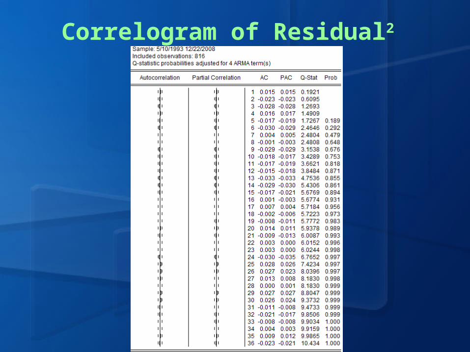
Correlogram of Residual2

Histogram
0
20
40
60
80
100
120
-2.50 -1.25 0.00 1.25 2.50 3.75 5.00
Series: Standardized ResidualsSample 5/10/1993 12/22/2008Observations 816
Mean 0.048932Median -0.086097Maximum 5.942007Minimum -2.775767Std. Dev. 0.999207Skewness 1.024413Kurtosis 6.494198
Jarque-Bera 557.8417Probability 0.000000

ARCH Test
ARCH Test:
F-statistic 0.190541 Prob. F(1,812) 0.662583
Obs*R-squared 0.190965 Prob. Chi-Square(1) 0.662115

Forecast
-.12
-.08
-.04
.00
.04
.08
.12
2008M07 2008M10 2009M01 2009M04
DLNPRICEF1DLNPRICEF1+2*SEFDLNPRICEF1-2*SEFDLNPRICE

Forecast

Recolor
100
150
200
250
300
350
400
450
08M01 08M04 08M07 08M10 09M01 09M04
LOWERUPPER
PRICEFPRICE

Comparison
100
150
200
250
300
350
400
450
08M01 08M04 08M07 08M10 09M01 09M04
PRICEALOWER
UPPERPRICEF
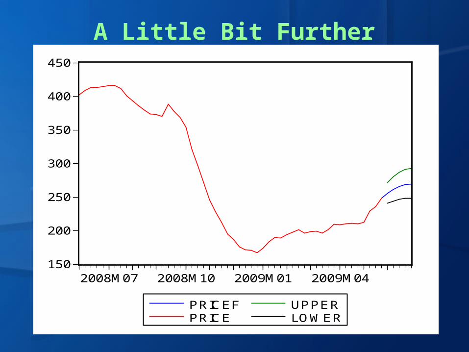
A Little Bit Further
-.12
-.08
-.04
.00
.04
.08
.12
2008M07 2008M10 2009M01 2009M04
DLNPRICEF1+2*SEFDLNPRICEF1-2*SEFDLNPRICEF1DLNPRICE
150
200
250
300
350
400
450
2008M07 2008M10 2009M01 2009M04
PRICEFPRICE
UPPERLOWER

Story Behind the Scene
To Investigate the Sources of Shock Geopolitical Events (War & Disasters)
GDP / Mean Personal Income
Vehicle Sales (SUV Sales)
China Petro Consumption
Speculation (Future Contract Price)
Key Bibliography “Causes and Consequences of the Oil Shock of 2007-08”
James D. Hamilton, UCSD (2009)


