Scientiae Mathematicae Japonicae Online, e-2004, 251–262 251

SPIRAL TRANSITION CURVES AND THEIR APPLICATIONS

Zulfiqar Habib and Manabu Sakai

Received August 21, 2003

Abstract. A method for family of G2 planar cubic Bezier spiral transition from

straight line to circle is discussed in this paper. This method is then extended to apair of spirals between two straight lines or two circles. We derive a family of cubictransition spiral curves joining them. Due to flexibility and wide range of shape controlparameters, our method can be easily applied for practical applications like high waydesigning, blending in CAD, consumer products such as ping-pong paddles, roundingcorners, or designing a smooth path that avoids obstacles.

1 Introduction A method for smooth G2 planar cubic Bezier spiral transition fromstraight line to circle is developed. This method is then extended to a pair of spirals tran-sition between two circles or between two non-parallel straight lines. We also derive anupper bound for shape control parameter and develop a method for drawing a constrainedguided planar spiral curve that falls within a closed boundary. The boundary is composedof straight line segments and circular arcs. Our constrained curve can easily be controlledby shape control parameter. Any change in this shape control parameter does not effect thecontinuity and neighborhood parts of the curve. There are several problems whose solutionrequires these types of methods. For example:

• Transition curves can be used for blending in the plane, i.e., to round corners, or forsmooth transition between circles or straight lines.• Consumer products such as ping-pong paddles or vase cross section can be designed byblending circles.• User can easily design rounding shapes like satellite antenna by surface of revolution ofour smooth transition curve.• For applications such as the design of highways or railways it is desirable that transitionsbe fair. In the discussion about geometric design standards in AASHO (American Associa-tion of State Highway officials), Hickerson [7] (p. 17) states that “Sudden changes betweencurves of widely different radii or between long tangents and sharp curves should be avoidedby the use of curves of gradually increasing or decreasing radii without at the same timeintroducing an appearance of forced alignment”. The importance of this design feature ishighlighted in [2] that links vehicle accidents to inconsistency in highway geometric design.• A user may wish to design a curve that fits inside a given region as, for example, whenone is designing a shape to be cut from a flat sheet of material.• A user may wish to design a smooth path that avoids obstacles as, for example, when oneis designing a robot or auto drive car path.

Parametric cubic curves are popular in CAD applications because they are the low-est degree polynomial curves that allow inflection points (where curvature is zero), so they

2000 Mathematics Subject Classification. 65D07, 65D10, 65D17, 65D18.Key words and phrases. G2 continuity; Spiral; Spline; Cubic Bezier; Curvature; Mathematica.

252 ZULFIQAR HABIB AND MANABU SAKAI

are suitable for the composition of G2 blending curves. To be visually pleasing it is desir-able that the blend be fair. The Bezier form of a parametric cubic curve is usually usedin CAD/CAM and CAGD (Computer Aided Geometric Design) applications because of itsgeometric and numerical properties. Many authors have advocated their use in differentapplications like data fitting and font designing. The importance of using fair curves in thedesign process is well documented in the literature [1, 10].

Cubic curves, although smoother, are not always helpful since they might have unwantedinflection points and singularities (See [3, 9]). Spirals have several advantages of containingneither inflection points, singularities nor curvature extrema (See [5, 4, 13]). Such curvesare useful for transition between straight lines and circles. Walton [11] considered a planarG2 cubic transition spiral joining a straight line and a circle. Its use enables us to join twocircles forming C- and S-shaped curves such that all points of contact are G2. Recently,Meek [8] presented a method for drawing a guided G1 continuous planar spline curve thatfalls within a closed boundary composed of straight line segments and circles. The objec-tives and shape features of our scheme in this paper are:

• To obtain a family of fair G2 cubic transition spiral curve joining a straight line anda circle.• To obtain a family of transition curves between two circles or between two non parallelstraight lines.• To simplify and extend the analysis of Walton [11].• To achieve more degrees of freedom and flexible constraints for easy use in practical ap-plications.• To find the upper bound for shape control parameter specially for guided G2 continuousspiral spline that falls within a closed boundary composed of straight line segments andcircles. Our guided curve has better smoothness than Meek [8] scheme which has G1 con-tinuity.• Any change in shape parameter does not effect continuity and neighborhood parts of ourguided spline. So, our scheme is completely local.

The organization of our paper is as follows. Next section gives a brief discussion ofthe notation and conventions for the cubic Bezier spiral with some theoretical backgroundand description of method. Its use for the various transitions encountered in general curve,guided curve and practical applications is analysed followed by illustrative examples, con-cluding remarks and future research work.

C

W

q

O

r

z(0)

z(1)

L

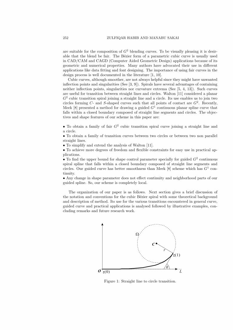
Figure 1: Straight line to circle transition.

SPIRAL TRANSITION CURVES AND THEIR APPLICATIONS 253

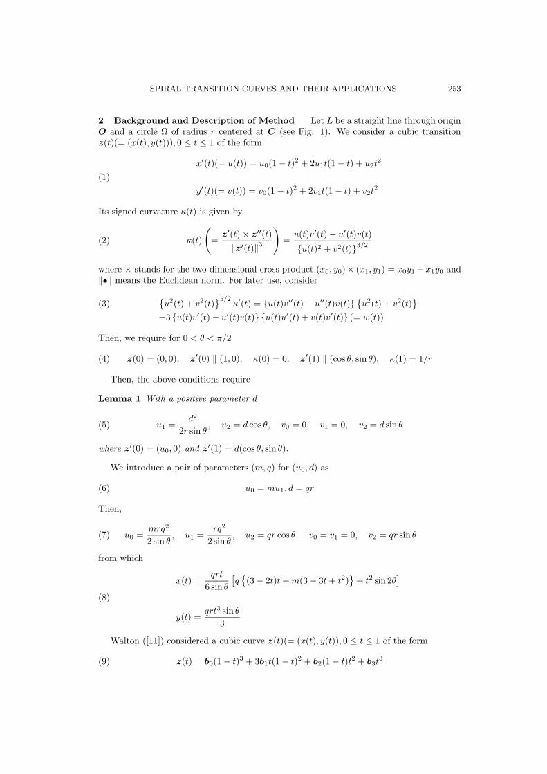
2 Background and Description of Method Let L be a straight line through originO and a circle Ω of radius r centered at C (see Fig. 1). We consider a cubic transitionz(t)(= (x(t), y(t))), 0 ≤ t ≤ 1 of the form

x′(t)(= u(t)) = u0(1 − t)2 + 2u1t(1 − t) + u2t2

(1)

y′(t)(= v(t)) = v0(1 − t)2 + 2v1t(1 − t) + v2t2

Its signed curvature κ(t) is given by

(2) κ(t)

(

=z′(t) × z

′′(t)

‖z′(t)‖3

)

=u(t)v′(t) − u′(t)v(t)

u(t)2 + v2(t)3/2

where × stands for the two-dimensional cross product (x0, y0)× (x1, y1) = x0y1 − x1y0 and‖•‖ means the Euclidean norm. For later use, consider

u2(t) + v2(t)5/2

κ′(t) = u(t)v′′(t) − u′′(t)v(t)

u2(t) + v2(t)

(3)

−3 u(t)v′(t) − u′(t)v(t) u(t)u′(t) + v(t)v′(t) (= w(t))

Then, we require for 0 < θ < π/2

(4) z(0) = (0, 0), z′(0) ‖ (1, 0), κ(0) = 0, z

′(1) ‖ (cos θ, sin θ), κ(1) = 1/r

Then, the above conditions require

Lemma 1 With a positive parameter d

(5) u1 =d2

2r sin θ, u2 = d cos θ, v0 = 0, v1 = 0, v2 = d sin θ

where z′(0) = (u0, 0) and z

′(1) = d(cos θ, sin θ).

We introduce a pair of parameters (m, q) for (u0, d) as

(6) u0 = mu1, d = qr

Then,

u0 =mrq2

2 sin θ, u1 =

rq2

2 sin θ, u2 = qr cos θ, v0 = v1 = 0, v2 = qr sin θ(7)

from which

x(t) =qrt

6 sin θ

[

q

(3 − 2t)t + m(3 − 3t + t2)

+ t2 sin 2θ]

(8)

y(t) =qrt3 sin θ

3

Walton ([11]) considered a cubic curve z(t)(= (x(t), y(t)), 0 ≤ t ≤ 1 of the form

(9) z(t) = b0(1 − t)3 + 3b1t(1 − t)2 + b2(1 − t)t2 + b3t3

254 ZULFIQAR HABIB AND MANABU SAKAI

where Bezier points bi, 0 ≤ i ≤ 3 are defined as follows

(10) b1 − b0 = b2 − b1 =25r tan θ

54 cos θ(1, 0), b3 − b2 =

5r tan θ

9(cos θ, sin θ)

Simple calculation gives

x′(t)(= u(t)) = u0(1 − t)2 + 2u1t(1 − t) + u2t2

(11)

y′(t)(= v(t)) = v0(1 − t)2 + 2v1t(1 − t) + v2t2

where

(12) u0 = u1 =25r tan θ

18 cos θ, u2 =

5r sin θ

3, v0 = v1 = 0, v2 =

5r tan θ sin θ

3

Hence, note that their method is our special case with m = 1 and q = 5 tan θ/3.With help of a symbolic manipulator, we obtain

(13) κ′

(

1

1 + s

)

=

8(1 + s)5(

5∑

i=0

aisi

)

sin3 θ

r

q2s2(2 + ms)2 + 2qs(2 + ms) sin 2θ + 4 sin2 θ5/2

where

a0 = 4 3q cos θ − (4 + m) sin θ sin θ, a1 = 2

6q2 − q(5 − 4m) sin 2θ − 10m sin2 θ

a2 = 2q (−2 + 13m)q − 2m(4 − m) sin 2θ , a3 = 2mq (−3 + 10m)q − 2m sin 2θa4 = 5m3q2, a5 = m3q2

Hence, we have a sufficient spiral condition for a transition curve z(t), 0 ≤ t ≤ 1, i.e.,ai ≥ 0, 0 ≤ i ≤ 5:

Lemma 2 The cubic segment z(t), 0 ≤ t ≤ 1 of the form (1) is a spiral satisfying (5) ifm > 3/10 and

q ≥ q(m, θ)

(

= Max

[

(4 + m) tan θ

3,

2m(4 − m) sin 2θ

13m − 2,

2m sin 2θ

10m − 3,

1

6

(5 − 4m) cos θ +√

60m + (5 − 4m)2 cos2 θ

sin θ

])

(14)

As in [11], we can require an additional condition κ′(1) = 0. Then a0 = 0, i.e., q =4+m

3tan θ. Therefore the above condition (14) gives a spiral one:

Lemma 3 The cubic segment z(t), 0 ≤ t ≤ 1 of the form (1) is a spiral satisfying (5) andκ′(1) = 0 for θ ∈ (0, π/2] if m ≥ 2(−1 +

√6)/5(= c0)(≈ 0.5797)

Proof. Letting z = tan θ(> 0), we only have to notice that the terms in brackets of (13)reduce

(4 + m)z

3(= A1),

4m(4 − m)z

(13m − 2)(1 + z2)(= A2),

4mz

(10m − 3)(1 + z2)(= A3),

z

5 − 4m +√

25 + 16m2 + 20m(1 + 3z2)

6(1 + z2)(= A4)

SPIRAL TRANSITION CURVES AND THEIR APPLICATIONS 255

Here, we have to check that the first quantity is not less than the remaining three oneswhere

A1 ≥ A2 (m ≥ 1

25(−1 +

√201)(≈ 0.5270))

A1 ≥ A3 (m ≥ 1

20(−25 +

√1105)(≈ 0.4120))

A1 ≥ A4 (m ≥ c0)

2.1 Circle to Circle Spiral Transition A method for straight line to circle transitionis being extended to C- or S-shaped transition between two circles Ω, Ω with centers C0,C1 and radii r0, r1 respectively. Now, z(t, r)(= (x(t, r), y(t, r)), 0 ≤ t ≤ 1 denotes thecubic spline satisfying (5). Then, a C-shaped pair of cubic curves: (x(t, r0), y(t, r0)) and(−x(t, r1), y(t, r1)) is considered to be a pair of spiral transition curves joining two circleswith radii r0, r1, respectively. Then, the distance ρ(= ‖C0 − C1‖) of the centers of the twocircles is given with q ≥ q(m, θ)

(15) ρ =√

g21(r0 + r1)2 + g2

2(r0 − r1)2

where

g1(= g1(m, θ, q)) =

(

1

6 sin θ

)

(1 + m)q2 + q sin 2θ − 6 sin2 θ

g2(= g2(m, θ, q)) =1

3(q sin θ + 3 cos θ)(16)

A simple calculation gives

(i) (g1(m, θ, q(m, θ)), g2(m, θ, q(m, θ))) → (0, 1) (θ → 0)

(17)

(ii) g1(m, θ, q(m, θ)), g2(m, θ, q(m, θ)) → ∞ (θ → π

2)

Hence we have

Theorem 1 If ‖C0 − C1‖ > |r0 − r1|, a C-shaped pair of cubic curves (x(t, r0), y(t, r0))and (−x(t, r1), y(t, r1)) is a pair of spiral transitions of G2-continuity from Ω to Ω for aselection of θ ∈ (0, π/2).

Next, a pair of an S-shaped cubic curves (x(t, r0), y(t, r0)) and (−x(t, r1),−y(t, r1)) isconsidered to be a pair of spiral transition curves from Ω to Ω. Then, the distanceρ(= ‖C0 − C1‖) of the centers of the two circles is given by

(18) ρ =√

g21 + g2

2(r0 + r1)

Note (16) to obtain

Theorem 2 If ‖C0 − C1‖ > r0 + r1, an S-shaped pair of cubic curves (x(t, r0), y(t, r0))and (−x(t, r1),−y(t, r1)) is a pair of spiral transitions of G2-continuity from Ω to Ω fora selection of θ ∈ (0, π/2).

256 ZULFIQAR HABIB AND MANABU SAKAI

q qg

r

C

W

O

P0

P1

d0d

1

P

Figure 2: Transition between two straight lines.

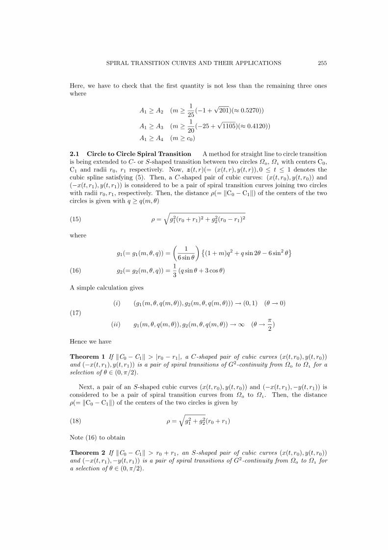
2.2 Straight Line to Straight Line Spiral Transition Here, we have extendedthe idea of straight line to circle transition and derived a method for Bezier spiral transitionbetween two nonparallel straight lines (see Fig. 2). We note the following result that is ofuse for joining two lines. For 0 < θ < π/2, we consider a cubic curve satisfying

(19) z(0) = (0, 0), z′(0) ‖ (1, 0), κ(0) = 1/r, z

′(1) ‖ (cos θ, sin θ), κ(1) = 0

Since Bezier curves are affine invariant, a cubic Bezier spiral can be used in a coordinatefree manner. Therefore transformation, i.e., rotation, translation, reflection with respect toy-axis and change of variable t with 1 − t to (9) gives z(t)(= (x(t), y(t)) by

x(t) =qrt

6 sin θ

[

qt 3 − (2 − m)t cos θ + 2(3 − 3t + t2) sin θ]

(20)

y(t) =q2rt2

63 − (2 − m)t

Now, z(t,m, θ)(= (x(t,m, θ), y(t,m, θ)), 0 ≤ t ≤ 1 denotes the cubic spline satisfying (19).Assume that the angle between two lines is γ (< π). Then, (x(t,m, θ0), y(t,m, θ0)) ofthe form (21) with q = q0(≥ q(m, θ0)) and (−x(t, n, θ1), y(t, n, θ1)) of the form (21) withq1(≥ q(n, θ1)) with θ0 + θ1 = π − γ is a pair of spiral transition curves whose join isG3. In addition, when θ0 = θ1 (= θ = (π − γ)/2) are fixed and m,n ≥ c0 (then, noteq0 = (4 + m)/3 tan θ and q1 = (4 + n)/3 tan θ), the distances between the intersection O

of the two lines and the the end points P i, i = 0, 1 of the transition curves are given byd(m,n, r, θ) and d(n,m, r, θ) where

(21) d(m,n, r, θ) = (r/c)

4 + (3 + m)3 + 3(3 + n)

, c = 54 cos2 θ/ sin θ

Here we derive a condition on r for which the following system of equations has the solutionsm,n(≥ c0) for given nonnegative d0, d1:

(22) d(m,n, r, θ) = d0, d(n,m, r, θ) = d1

Let (α, β) = (3 + m, 3 + n) reduce the above system to

(23) α3 + 3β = λ(= cd0/r − 4), β3 + 3α = µ(= cd1/r − 4)

where require m,n ≥ c0 to note α, β ≥ c1(= c0 + 3) and λ, µ ≥ c2(= c31 + 3c1). Delete α

from (1.23) to get a quartic equation f(β) = 0:

(24) f(β) = β9 − 3µβ6 + 3µ2β3 − 81β + 27λ − µ3

SPIRAL TRANSITION CURVES AND THEIR APPLICATIONS 257

Restrictions: α, β ≥ c1 require that at least one root β of f(β) = 0 must satisfy

(25) c1 ≤ β ≤ (µ − 3c1)1/3

Intermediate value of theorem gives a sufficient condition: f(c1) ≤ 0 and f((µ − 3c1)1/3) ≥ 0

where

f(c1) = −µ3 + 3c31µ

2 − 3c61µ + 27λ + c9

1 − 81c1 = −

µ − c31 − 3(λ − 3c1)

1/3

×[

(µ − c2)2 + 3

2c1 + (λ − 3c1)1/3

(µ − c2) + 9

c21 + c1(λ − 3c1)

1/3 + (λ − 3c1)2/3

]

(26)

f((µ − 3c1)1/3) = 27

λ − c31 − 3(µ − 3c1)

1/3

Since the quantity in brackets is positive for µ ≥ c2, the sufficient one reduces to

(27) λ − c31 ≥ 3(µ − 3c1)

1/3, µ − c31 ≥ 3(λ − 3c1)

1/3

Note λ, µ ≥ c2 to obtain

Lemma 4 Given d0, d1, assume that r satisfies λ − c31 ≥ 3(µ − 3c1)

1/3 ≥ 0, µ − c31 ≥

3(λ − 3c1)1/3 ≥ 0. Then the system of (23) has the required solutions α, β (≥ c1).

Note λ, µ = O(1/r), r → 0 to obtain that a small value of r makes the inequalities (27) bevalid for any d0, d1. Next, for an upper bound for r, we require

Lemma 5 If d0 ≥ d1, then µ − c31 = 3(λ − 3c1)

1/3 and λ, µ ≥ c2 by (23) has a uniquepositive solution r∗.

Proof. Let t = 1/r to reduce µ − c31 = 3(λ − 3c1)

1/3 to

(28) f(t)(

= (cd1t − 4 − c31)

3 − 27(cd0t − 4 − 3c1))

= 0

where λ, µ ≥ c2 are equivalent to t ≥ (c2 + 4)/(cd1). First, note with d0 = k2d1 (k ≥ 1)

f(+∞) = +∞, f

(

c2 + 4

cd1

)

= −27(c1 + 1)(c21 − c1 + 4)(k2 − 1)(≤ 0)

In addition, f(t) has its relative maximum at t = (c31 + 4 − 3k)/(cd1) (< (c2 + 4)/(cd1)).

Therefore, f(t) = 0 has just one root t = t∗(= 1/r∗) (≥ (c2 + 4)/(cd1)). As r increases from

zero, ’equality” in the second inequality of (27) is first valid. Hence, we obtain

Theorem 3 Assume that d0 ≥ d1. Then the system of equation (22) in m,n (≥ c0) issolvable for 0 < r ≤ r∗ where r∗ is the positive root no greater than cd1/(c2 + 4):

(4 + c31)r − cd1

3 − 27r2 (4 + 3c1)r − cd0 = 0, c1 = c30 + 3c0(29)

Then, for the angle γ (< π) between the two straight lines with θ = (π − γ)/2, (x(t,m, θ),y(t,m, θ)), q = (4 + m)/3 tan θ of the form (21) and (−x(t, n, θ), y(t, n, θ)), q = (4 + n)/3 tan θof the form (21) is a pair of spiral transition curves between the two lines.

This result enables the pair of the spirals to pass through the given points of contact onthe non-parallel two straight lines. For example, Lemma 4 shows that for γ = π/3 and(d0, d1) = (3, 1) (Figure 8 in Numerical Example), r∗ ≈ 0.2326. For fixed θ, r∗ could beenlarged as follows. That is, for θ = π/3, we only have to notice q(m, θ) = (4 + m)/3 tan θ

258 ZULFIQAR HABIB AND MANABU SAKAI

-4 -2 2

0.51

1.52

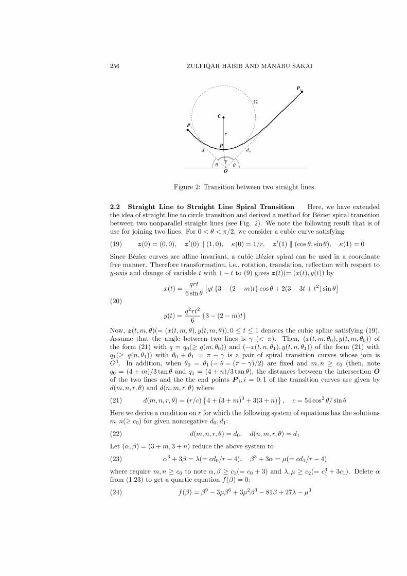
Figure 3: Graphs of z(t) with (r0, r1, θ) = (0.5, 1, π/3).

-4 -2 2

-2.5-2

-1.5-1

-0.5

0.51

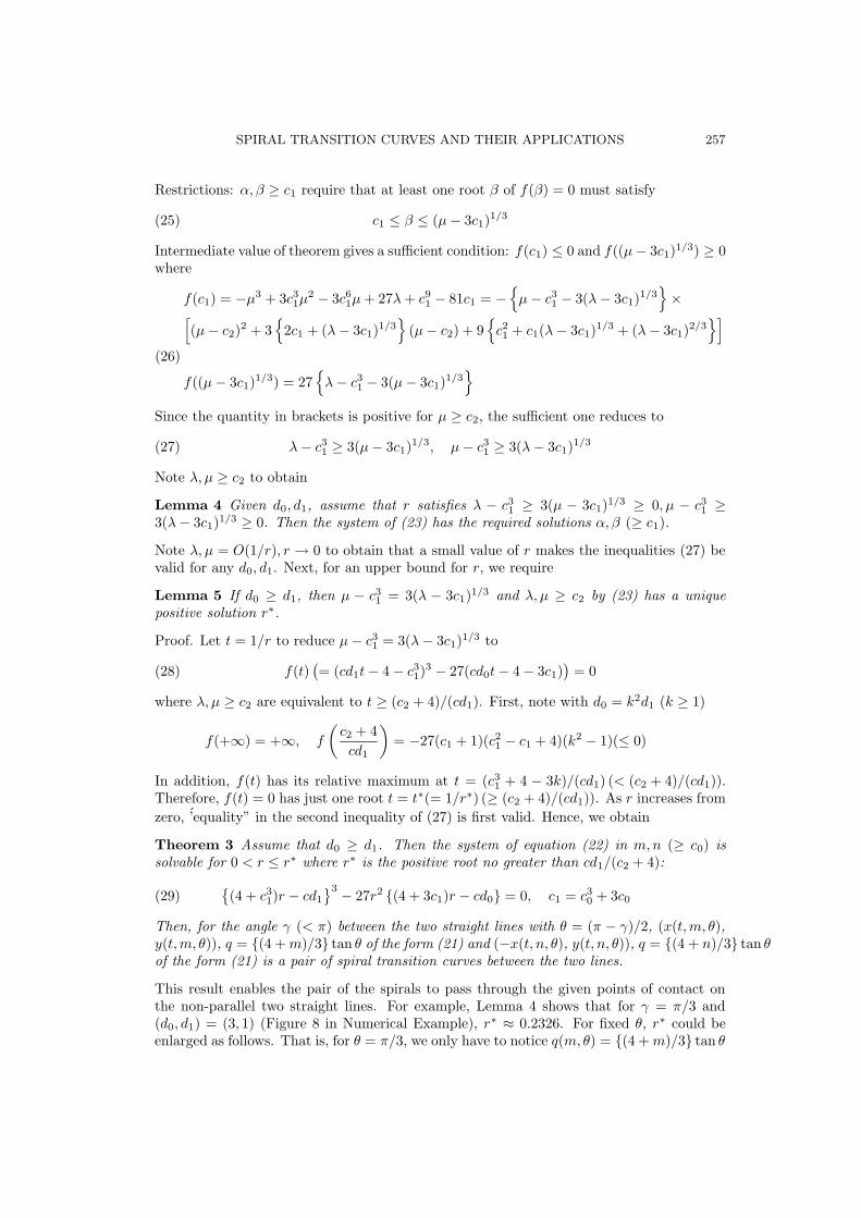
Figure 4: Graphs of z(t) with (r0, r1, θ) = (0.5, 1, π/3).

-3 -2 -1 1

0.5

1

1.5

2

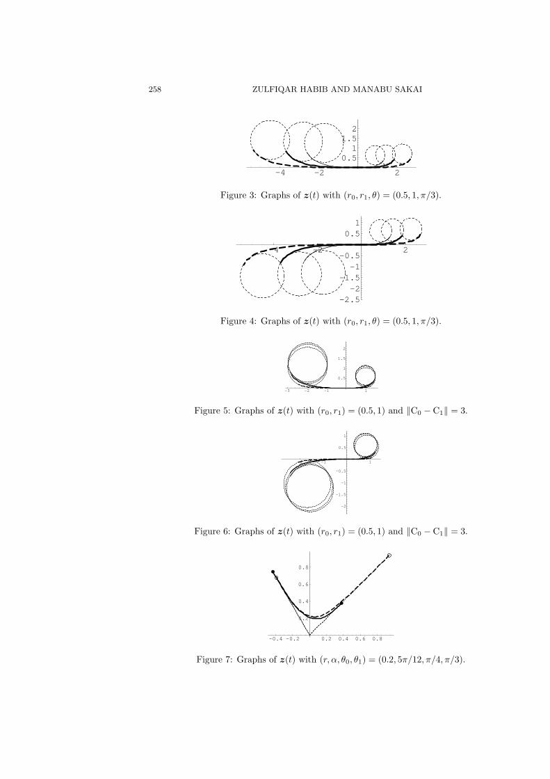
Figure 5: Graphs of z(t) with (r0, r1) = (0.5, 1) and ‖C0 − C1‖ = 3.

-2 -1 1

-2

-1.5

-1

-0.5

0.5

1

Figure 6: Graphs of z(t) with (r0, r1) = (0.5, 1) and ‖C0 − C1‖ = 3.

-0.4 -0.2 0.2 0.4 0.6 0.8

0.2

0.4

0.6

0.8

Figure 7: Graphs of z(t) with (r, α, θ0, θ1) = (0.2, 5π/12, π/4, π/3).

SPIRAL TRANSITION CURVES AND THEIR APPLICATIONS 259

for m ≥ c0 = (√

409 − 17)/10(≈ 0.3223) instead of m ≥ c0(≈ 0.5797). Then, for(d0, d1) = (3, 1), r∗ ≈ 0.2742 with (m,n) ≈ (2.38, 0.32).

Finally we remark the next result for the limiting case (r → 0):

(30) P =r

18

(

(m − n) tan θ,−(8 + m + n) tan2 θ)

→ O(= (0, 0))

since r → 0 gives m,n = O(

r−1/3)

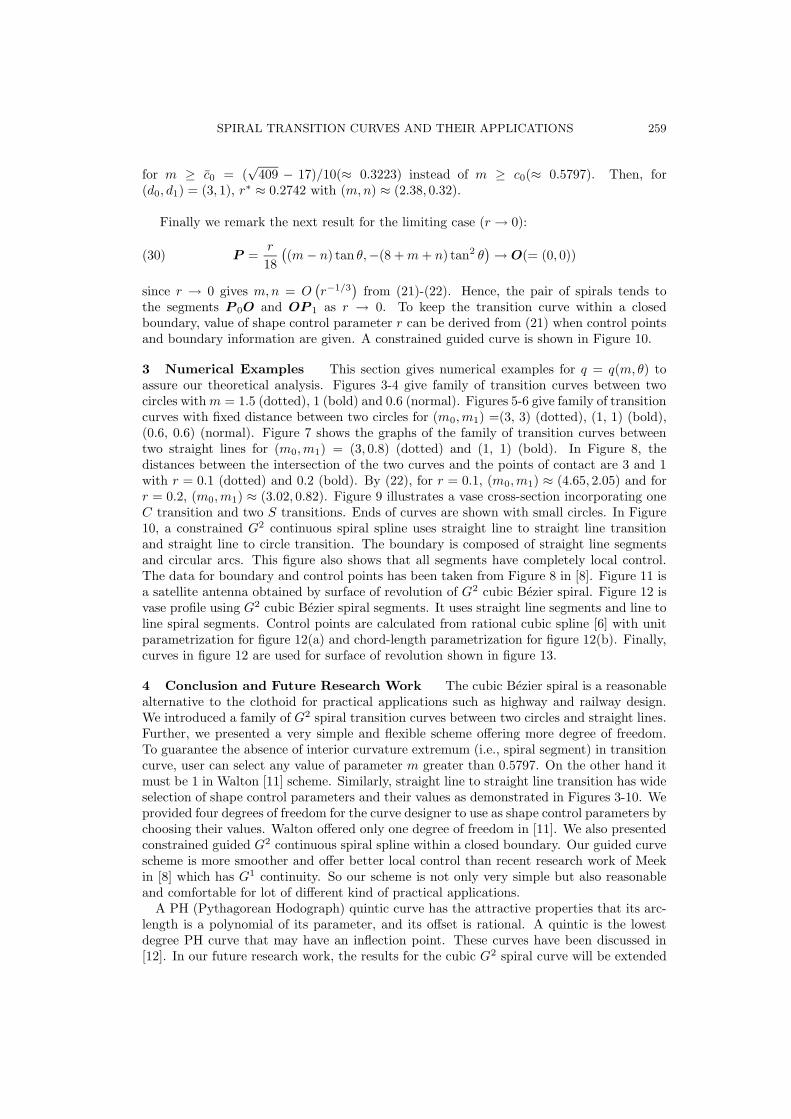
from (21)-(22). Hence, the pair of spirals tends tothe segments P 0O and OP 1 as r → 0. To keep the transition curve within a closedboundary, value of shape control parameter r can be derived from (21) when control pointsand boundary information are given. A constrained guided curve is shown in Figure 10.

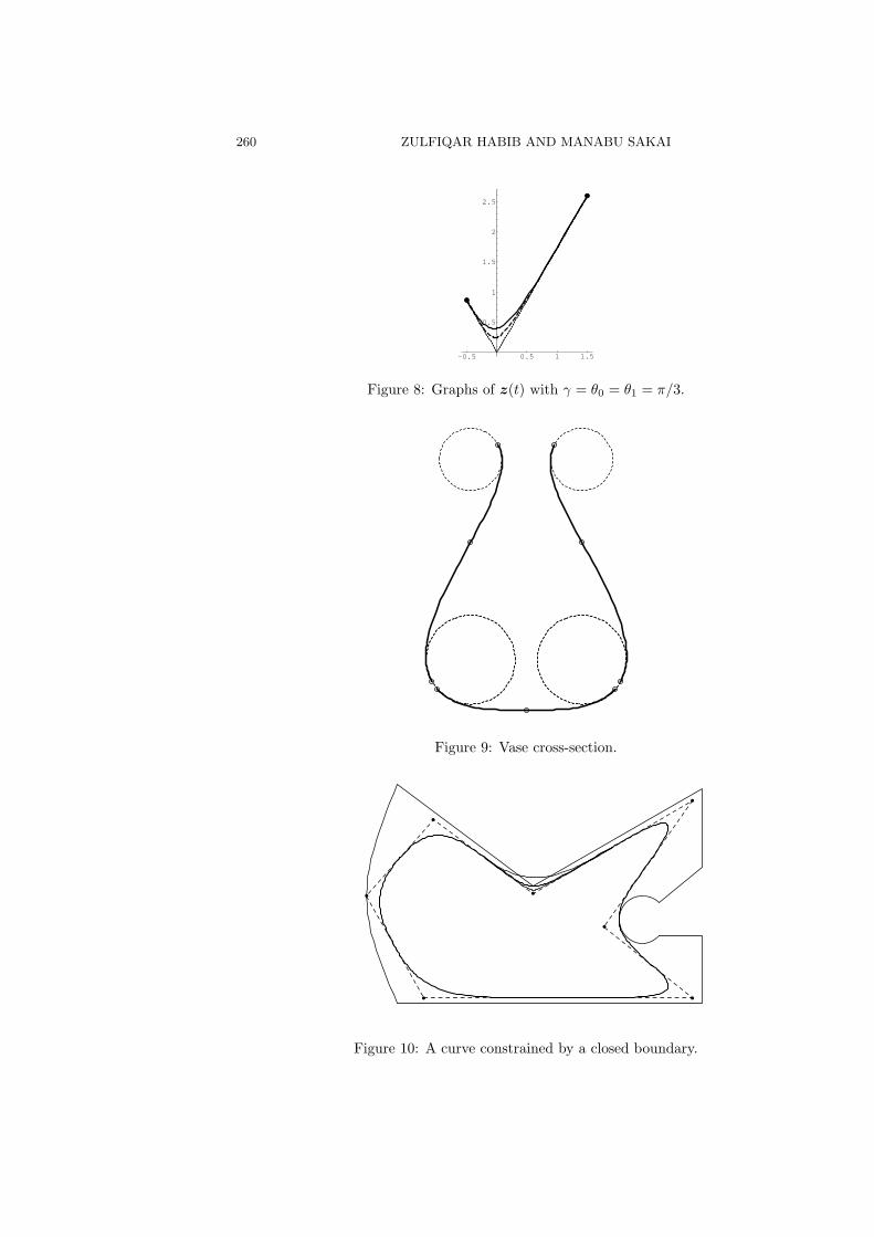
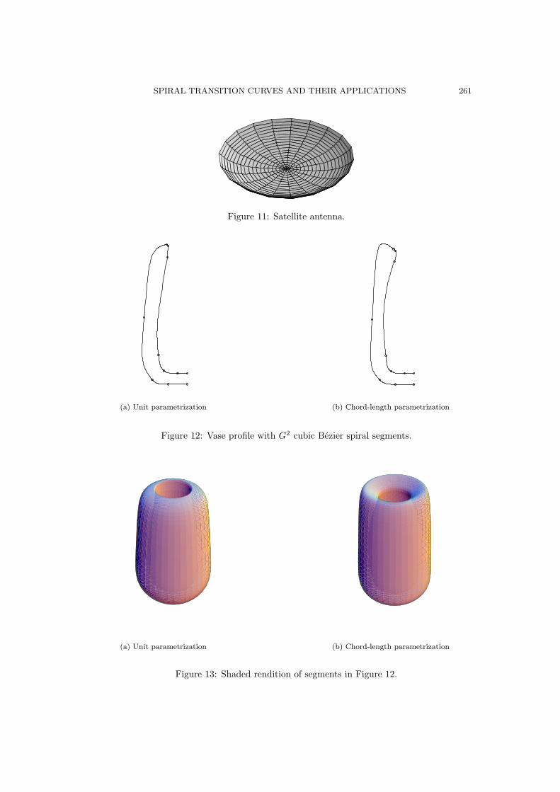
3 Numerical Examples This section gives numerical examples for q = q(m, θ) toassure our theoretical analysis. Figures 3-4 give family of transition curves between twocircles with m = 1.5 (dotted), 1 (bold) and 0.6 (normal). Figures 5-6 give family of transitioncurves with fixed distance between two circles for (m0,m1) =(3, 3) (dotted), (1, 1) (bold),(0.6, 0.6) (normal). Figure 7 shows the graphs of the family of transition curves betweentwo straight lines for (m0,m1) = (3, 0.8) (dotted) and (1, 1) (bold). In Figure 8, thedistances between the intersection of the two curves and the points of contact are 3 and 1with r = 0.1 (dotted) and 0.2 (bold). By (22), for r = 0.1, (m0,m1) ≈ (4.65, 2.05) and forr = 0.2, (m0,m1) ≈ (3.02, 0.82). Figure 9 illustrates a vase cross-section incorporating oneC transition and two S transitions. Ends of curves are shown with small circles. In Figure10, a constrained G2 continuous spiral spline uses straight line to straight line transitionand straight line to circle transition. The boundary is composed of straight line segmentsand circular arcs. This figure also shows that all segments have completely local control.The data for boundary and control points has been taken from Figure 8 in [8]. Figure 11 isa satellite antenna obtained by surface of revolution of G2 cubic Bezier spiral. Figure 12 isvase profile using G2 cubic Bezier spiral segments. It uses straight line segments and line toline spiral segments. Control points are calculated from rational cubic spline [6] with unitparametrization for figure 12(a) and chord-length parametrization for figure 12(b). Finally,curves in figure 12 are used for surface of revolution shown in figure 13.

4 Conclusion and Future Research Work The cubic Bezier spiral is a reasonablealternative to the clothoid for practical applications such as highway and railway design.We introduced a family of G2 spiral transition curves between two circles and straight lines.Further, we presented a very simple and flexible scheme offering more degree of freedom.To guarantee the absence of interior curvature extremum (i.e., spiral segment) in transitioncurve, user can select any value of parameter m greater than 0.5797. On the other hand itmust be 1 in Walton [11] scheme. Similarly, straight line to straight line transition has wideselection of shape control parameters and their values as demonstrated in Figures 3-10. Weprovided four degrees of freedom for the curve designer to use as shape control parameters bychoosing their values. Walton offered only one degree of freedom in [11]. We also presentedconstrained guided G2 continuous spiral spline within a closed boundary. Our guided curvescheme is more smoother and offer better local control than recent research work of Meekin [8] which has G1 continuity. So our scheme is not only very simple but also reasonableand comfortable for lot of different kind of practical applications.

A PH (Pythagorean Hodograph) quintic curve has the attractive properties that its arc-length is a polynomial of its parameter, and its offset is rational. A quintic is the lowestdegree PH curve that may have an inflection point. These curves have been discussed in[12]. In our future research work, the results for the cubic G2 spiral curve will be extended

260 ZULFIQAR HABIB AND MANABU SAKAI

-0.5 0.5 1 1.5

0.5

1

1.5

2

2.5

Figure 8: Graphs of z(t) with γ = θ0 = θ1 = π/3.

Figure 9: Vase cross-section.

Figure 10: A curve constrained by a closed boundary.

SPIRAL TRANSITION CURVES AND THEIR APPLICATIONS 261

Figure 11: Satellite antenna.

(a) Unit parametrization (b) Chord-length parametrization

Figure 12: Vase profile with G2 cubic Bezier spiral segments.

(a) Unit parametrization (b) Chord-length parametrization

Figure 13: Shaded rendition of segments in Figure 12.

262 ZULFIQAR HABIB AND MANABU SAKAI

to family of PH quintic G2 spiral transition curves. We will try for simplified and moreflexible shape parameter values.Acknowledgement

We acknowledge the financial support of JSPS (Japan Society for the Promotion ofScience).

References

[1] G. Farin. NURB Curves and Surfaces. A K Peters, 1995.

[2] G. M. Gibreel, S. M. Easa, Y. Hassan, and I. A. El-Dimeery. State of the art of highwaygeometric design consistency. ASCE Journal of Transportation Engineering, 125(4):305–313,1999.

[3] Z. Habib and M. Sakai. G2 two-point Hermite rational cubic interpolation. International

Journal of Computer Mathematics, 79(11):1225–1231, 2002.

[4] Z. Habib and M. Sakai. G2 planar cubic transition between two circles. International Journal

of Computer Mathematics, 80(8):959–967, 2003.

[5] Z. Habib and M. Sakai. Quadratic and T-cubic spline approximations to a pla-nar spiral. Scientiae Mathematicae Japonicae, 57(1):149–156, 2003. :e7, 107-114,http://www.jams.or.jp/scmjol/7.html.

[6] Z. Habib and M. Sarfraz. A rational cubic spline for the visualization of convex data. pages744–748, USA, July 2001. The Proceedings of IEEE International Conference on InformationVisualization-IV’01-UK, IEEE Computer Society Press.

[7] T. F. Hickerson. Route Location and Design. McGraw-Hill, New York, 1964.

[8] D. S. Meek, B. Ong, and D. J. Walton. A constrained guided G1 continuous spline curve.

Computer Aided Design, 35:591–599, 2003.

[9] M. Sakai. Osculatory interpolation. Computer Aided Geometric Design, 18:739–750, 2001.

[10] B. Su and D. Liu. Computaional Geometry: Curve and Surface Modeling. Academic Press,New York, 1989.

[11] D. J. Walton and D. S. Meek. A planar cubic Bezier spiral. Computational and Applied

Mathematics, 72:85–100, 1996.

[12] D. J. Walton and D. S. Meek. A Pythagorean hodograph quintic spiral. Computer Aided

Design, 28:943–950, 1996.

[13] D. J. Walton and D. S. Meek. Curvature extrema of planar parametric polynomial cubiccurves. Computational and Applied Mathematics, 134:69–83, 2001.

Department of Mathematics and Computer Science, Graduate School of Science and Engi-neering, Kagoshima University, Kagoshima 890-0065, Japan.Phone: ++81-99-2858049; Fax: ++81-99-2858051Email: habib@eniac.sci.kagoshima-u.ac.jp; msakai@sci.kagoshima-u.ac.jp