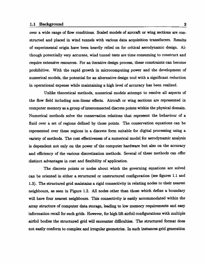
Adapt ive Solution of Viscous Aerodynamic Flows - TSpace

Adapt ive Solution of Viscous Aerodynamic Flows Using Unstructured Grids

Paul Charles Walsh

A thesis submitted in conformi@ with the requirements

for the degree of Doctor of Philomphy

Graduate Department of Aerospace Science and Engineering

University of Toronto

@Copyright by Paul Chsrles Walsh 1998

National Library Bibiioîhèque nationale du Canada

Acquisitions and Acquisitions et Bibliographie SeMces services bibliographiques

395 WeUingbDn Street 395. rue Wellington OttawaON K 1 A W Ottawa ON K1A OCJ4 canada CaMda

The author has granted a non- L'auteur a accordé une licence non exclusive licence allowing the exclusive permettant à la National Library of Canada to Bibliothèque nationale du Canada de reproduce, loan, distribute or sel1 reproduire, prêter, distribuer ou copies of this thesis in microfoq vendre des copies de cette thèse sous paper or electronic formats. la forme de microfiche/nlm, de

reproduction sur papier ou sur format électronique.

The author retains ownership of the L'auteur conserve la propriété du copyright in this thesis. Neither the droit d'auteur qui protège cette thèse. thesis nor substantial extracts ~ o m it Ni la thèse ni des extraits substantiels may be printed or otherwise de celle-ci ne doivent être imprimés reproduced without the author's ou autrement reproduits sans son permission. autorisation.

Adaptive Solution of Viscous Aerodynamic Flows Using Unstructured Grids

Paul Charles Walsh

University of Toronto, Institute for Aerospace Studies

Doctor of Philosophy, 1998

Abstract

Unstnictured grids are used in numericd models applied to aerodynamic design

for their ability to conform easily to complex geometries. Their lack of rigid connectivity

d o m the grid generation process to be highly automated, reducing the expertise needed.

The ~n~tnict~red grid is idedy suited for bcal refinement basecl on the flow field solu-

tion, providing an opportunity for faster, less memory intensive operation for a specific

level of accuracy. The purpose of this research is to develop such an algorithin using

solution-adaptive unstmctured triangular grids to solve the compressible Navier-Stokes

equations on two-dimensiond airfoi1 profiles. The basic solver utilizes a finite-volume

methodology with Runge-Kutta time rnarching to produce steady-state solutions. An

improved artificid dissipation method is developed that provides reduced grid sensitiv-

ity and improved accuracy for high-aspect-ratio grids. The solution-adaptive gridding

method identifies under-resolved regions of the solution through an adaptation parameter

based on nomalized grid edge différences of the flow field variables. New grid nodes are

added in regions where the magnitude of the adaptation parameter is greatest, yielding

a local grid refhement. The hi&-aspectratio nature of the grid in viscous regions of the

flow is preserved after adaptation through the development of a solutiondependent retri-

mgdation routine. Several test cases on laminar and turbulent flows are presented that

demonstrate the performmce of the algorithm. It is shown that the adaptation configu-

ration that achieves the greatest improvement in remlution uses an adaptation parameter

consisting of a combination of Mach number and densi@ edge differences, with 55% of the

adapted nodes added in the first pass and 45% in the second to yield a four-fold increase

in the number of grid nodes. The test cases also demonstrate that the adaptation rou-

tine is capable of providing at least a 40% reduction in Mt and pressure drag coefficient

errors over d flow regimes compared to solutions obtained on unadapted grids with an

equivalent number of nodes. The effectiveness of the algorithm as a design tool is realized

in a final cornparison of an adapted solution to experimentally determineci results on a

cornplex three-element airfoil configuration.

Acknowledgement s

1 wodd like to express my gratitude to my supervisor Dr. D.W. Zingg for his support

and inspiration throughout the development of this research and in the writing of this

thesis. 1 would also like to thank the other members of my doctoral cornmittee, Dr. J. J.

Gottlieb and Dr. J.S. Hansen for th& efforts and suggestions.

1 also wish to extend m y thanks to the N a t d Sciences and Engineering Re-

search Councü of Canada, the Goveniment of Ontario, and the University of Toronto for

providing funding which made this work possible.

During my studies at the Universi@ of Toronto my family and &ends provided

ready encouragement, which was indispensible in the completion of this research. To

them 1 offer my gratitude and appreciation. Findy, I would like to extend my sincerest

appreciation to Ruth Boehme for her unflagging support and assistance in the preparation

of this thesis.

Contents

Acknawledgement s iii

List of Tables vü

List of Figures ix

Nomenclature mri

1 Introduction 1

. . . . . . . . . . . . . . . . . . . . . . . . . . . . . . . . . . . 1.1 Background 1

. . . . . . . . . . . . . . . . . . . . . . . . . . . . . . . . 1.2 Literature Review 7

. . . . . . . . . . . . . . . . . . . . . . . . . . 1.2.1 Unstructureci Solvers 7

. . . . . . . . . . . . . . . . . . . . . . . . . . 1.2.2 Turbulence Modehg 12

. . . . . . . . . . . . . . . . . . . . . . . . . . . . . 1.2.3 Grid Generation 12

. . . . . . . . . . . . . . . . . . . . . . 1.2.4 Solution-Adaptive Gridding 13

. . . . . . . . . . . . . . . . . . . . . . . . . . . . . . . . . . . . 1.3 Objectives 16

. . . . . . . . . . . . . . . . . . . . . . . . . . . . . . 1.4 Document Ovewiew 17

2 Numerid Algorithm 19

. . . . . . . . . . . . . . . . . . . . . . . . . . . . . . 2.1 Governing Equations 19

. . . . . . . . . . . . . . . . . . . . . . . . . . . . . . 2.2 Turbulence Modelling 23

. . . . . . . . . . . . . . . . . . . . . . . . . . . . . . 2.3 Spatial Discretization 27

. . . 2.4 Temporal Discretization . . . . . . . . . . . . . . . . . . . . . . . ... 33

2.5 Boundary Conditions . . . . . . . . . . . . . . . . . . . . . . . . . . . . . . 37

2.5.1 Free Stream Conditions . . . . . . . . . . . . . . . . . . . . . . . . 37

2.5.2 Far-Field Boundary Conditions . . . . . . . . . . . . . . . . . . . . 38

2.5.3 Airfoil Surface Conditions . . . . . . . . . . . . . . . . . . . . . . . 41

2.6 Convergence Enhancement . . . . . . . . . . . . . . . . . . . . . . . . . . . 48

2.6.1 Local T h e Stepping . . . . . . . . . . . . . . . . . . . . . . . . . . 48

2.6.2 Residual Srnoothing . . . . . . . . . . . . . . . . . . . . . . . . . . 49

2.6.3 The Multigrid Method . . . . . . . . . . . . . . . . . . . . . . . . . 50

2.7 Grid Generation . . . . . . . . . . . . . . . . . . . . . . . . . . . . . . . . . 56

3 Artificial Dissipation 67

3.1 Motivation . . . . . . . . . . . . . . . . . . . . . . . . . . . . . . . . . . . . 67

3.2 Jarneson's Artiticial Dissipation . . . . . . . . . . . . . . . . . . . . . . . . 70

3.3 Stretched Artificial Dissipation . . . . . . . . . . . . . . . . . . . . . . . . 73

3.4 Higher Order Artificial Dissipation . . . . . . . . . . . . . . . . . . . . . . 75

3.5 Higher Order Stretched Dissipation . . . . . . . . . . . . . . . . . . . . . . 78

4 Solution Adaptation 84

. . . . . . . . . . . . . . . . . . . . . . . . . . . . . . . . . . . . 4.1 Motivation 84

. . . . . . . . . . . . . . . . . . . . . . . . . . . . . 4.2 Adaptation parameters 85

. . . . . . . . . . . . . . . . . . . . . . . . . . 4.3 Airfoil Boundary Adaptation 91

4.4 Solution Adaptive &trimgdation . . . . . . . . . . . . . . . . . . . . . . . 95

5 Resdts 101

5.1 TestCases . . . . . . . . . . . . . . . . . . . . . . . . . . . . . . . . . . . . 101 5.2 Casel: NACA 0012 . . . . . . . . . . . . . . . . . . . . . . . . . . . . . . . 103 5.3 Case 2: NACA 0012 . . . . . . . . . . . . . . . . . . . . . . . . . . . . . . 122 5.4 Case 3: NACA 0012 . . . . . . . . . . . . . . . . . . . . . . . . . . . . . . 130

5.5 Case 4: NACA 0012 . . . . . . . . . . . . . . . . . . . . . . . . . . . . . . 136 5.6 Case 5: RAE 2822 . . . . . . . . . . . . . - . . . . . . . . . . . . . . . . . 149 5.7 Case6: AGARDAR303A2 . . . . . . . . . . . . . . . . . . . . . . . . . 152

6 Conclusions, Contributions, and Recommendations 166

6.1 Conclusions . . . . . . . . . . . . . . . . . - - - . . . . . . . . . . . . . . . 166 6.2 Contributions . . . . - . . . . . . . . . . . . . . , . . . . . . . . . . . . . . 168 6.3 Recommendations . . . . . . . . . . . . . . . . . . . . . . . . . . . - . . . 169

A Spalart-niimnras Turbulence Mode1 183

List of Tables

2.1 Non-reflecting far-field boundary specifications . . . . . . . . . . . . . . . . 42

5.1 Test Case Summary . . . . . . . . . . . . . . . . . . . . . . . . . . . . . . . 101

5.2 Grid specifications for Case 1 . . . . . . . . . . . . . . . . . . . . . . . . . 103

5.3 Unadapted lift and drag r d t s for Case 1 . . . . . . . . . . . . . . . . . . 104

5.4 Percent error for unadapteci grid results . . . . . . . . . . . . . . . . . . . 116

5.5 Lift and drag resdts after adaptation of grid nacaal . . . . . . . . . . . . . 116

5.6 Percent error of lift and drag resuits after adaptation of grid nacaal . . . . 117

5.7 Lift and drag results after adaptation of @d nacaa2 . . . . . . . . . . . . . 117

. . . 5.8 Percent error for lift and drag results after adaptation of grid nacaa2 118

5.9 Lift and drag results after adaptation of grid nacaa3 . . . . . . . . . . . . . 118

. . . 5.10 Percent error for lift and drag results after adaptation of grid nacaa3 119

. . . . . . . . . . 5.11 Lift and drag results after two adaptations of grid nacaal 119

5.12 Percent error for lift and drag results after two adaptations of grid nacaal 119

. . . . . . . . . . . . . . . . . . . . . . . . . 5.13 Grid specifications for Case 2 122

. . . . . . . . . . . . . . . . . . . . 5.14 Drag results ushg lower order damping 124

5.15 Absolute value of the percent error of drag results ushg lower order dampingl24

5.16 Drag results using higher order dsmping . . . . . . . . . . . . . . . . . . . 124

5.17 Absolute d u e of the percent error of drag remilts using higher order dampingl25

5.18 Drag r d t s after adaptive gridding and higher order damping . . . . . . . 125

5.19 Absolute value of the drag error after adaptive gridding and higher order

damping . . . . . . . . . . . . . . . . . . . . . . . . . . . . . . . . . . . 125

5.20 Grid specifications for Case 3 . . . . . . . . . . . . . . . . . . . . . . . . . 130

5.21 Unadapted lift and drag results for Case 3 . . . . . . . . . . . . . . . . . . 132

5.22 Percent error for unadapted grid r d t s . . . . . . . . . . . . . . . . . . . 133

5.23 Percent error for adapted grid r d t s . . . . . . . . . . . . . . . . . . . . . 133

List of Figures

1.1 Exampie of a structured grid . . . . . . . . . . . . . . . . . . . . . . . . . . 4

1.2 Details of structured grid connectivity . . . . . . . . . . . . . . . . . . . . 4

1.3 ~ p l e o f a u n s t m c t u r e d g r i d . . . . . . . . . . . . . . . . . . . . . . . . 5

1.4 Details of unstructured grid connectivity . . . . . . . . . . . . . . . . . . . 5

1.5 Adapted grid for NACA 0012 airfoil . . . . . . . . . . . . . . . . . . . . . 6

1.6 Mach number field about a NACA 0012 airfoil, M, = 0.8, a = 10.OO, Re =

500 . . . . . . . . . . . . . . . . . . . . . . . . . . . . . . . . . . . 6

2.1 m p l e of a cell centered control volume about node k . . . . . . . . . . . 31

2.2 Example of a node centered control volume about node k with the control

. . . . . . . . . . . . . . . volume boundary indicated with the dashed line 32

2.3 Example of a control volume adjacent to the airfoil surface centered about

nodek . . . . . . . . . . . . . . . . . . . . . . . . . . . . . . . . . . . . . . 44

2.4 Mach number contours about a NACA 0012 at M,=O.S, cr=O.O, Re, =

5000 . . . . . . . . . . . . . . . . . . . . . . . . . . . . . . . . . . . . . . . 45

2.5 Mach number profile at ~0.70 on the upper airfoil surfme . . . . . . . . . 46

2.6 Temperature profile at z=0.?0 on the upper airfoi1 surf'hce . . . . . . . . . 46

2.7 Enlargement of the temperature profile near the airfoil d a c e . . . . . . . 47

2.8 Density prose at -0.70 on the upper airfoil d a c e . . . . . . . . . . . . 47

2.9 Pressure profile at x=0.70 on the upper aidoil surface . . . . . . . . . . . 48 2.10 Example of a high and low fiequency error on a 1-D grid showing the

appwance of the low frequency error after transfer to the coarse grid . . . 52

2.11 The saw-tooth multigrid cycle development on a series of three gr&. . . . 54

2.12 Portion of a sample coarse and h e grid showing overlapping triangles . . . 55

2.13 Airfoil d a c e nodes showing Steiner vectors and gradations of off-wall

spacing . . . . . . . . . . . . . . . . . . . . . . . . . . . . . . . . . - . . . . 60

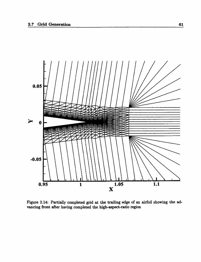
2.14 Partidy completed grid at the trailing edge of an airfoi1 showing the ad-

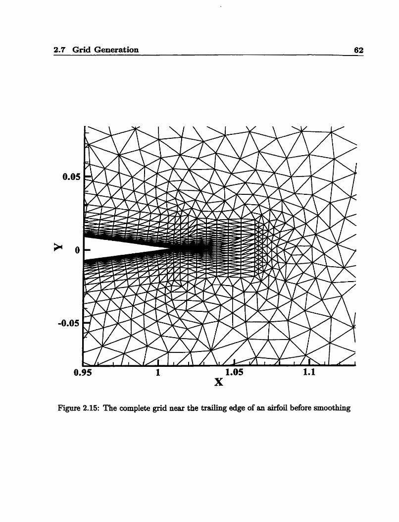
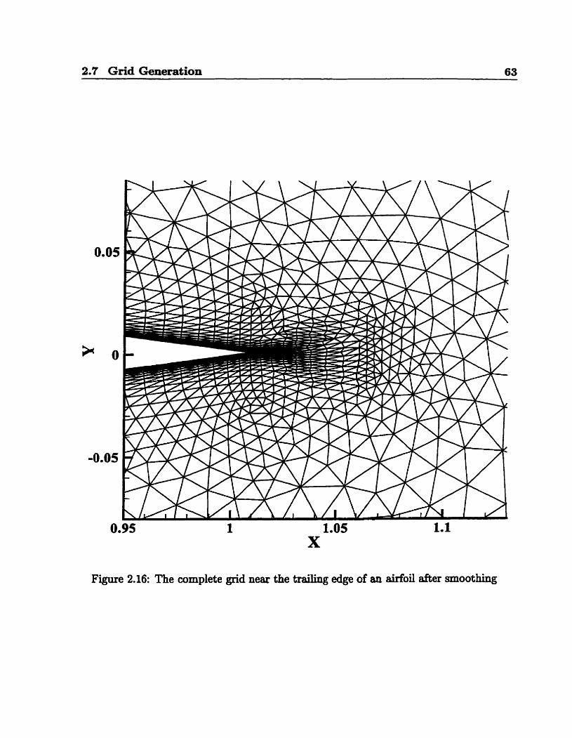
vancing &ont after having completed the high-aspect-ratio region . . . . . 61 2.15 The complete grid near the traüing edge of an airfoi1 before smoothing . . 62 2.16 The complete grid near the trailing edge of an airfoil after smoothing . . . 63

2.17 Example of a complete unstructured grid . . . . . . . . . . . . . . . . . . . 64 2.18 ~nstmctured grid near an airfoil surface . . . . . . . . . . . . . . . . . . . 65

2.19 'Eansition fiom near quilateral triangles to high-aspect-ratio at the leading

edge of an aidoil . . . . . . . . . . . . . . . . . . . . . . . . . . . . . . . . 66

One error mode possible on an unstructured grid; A and B are different

values of the local solution . . . . . . . . . . . . . . . . . . . . . . . . . . . 69

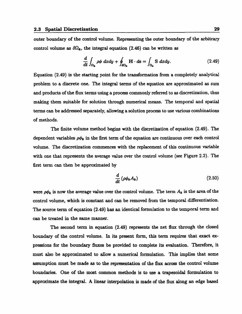
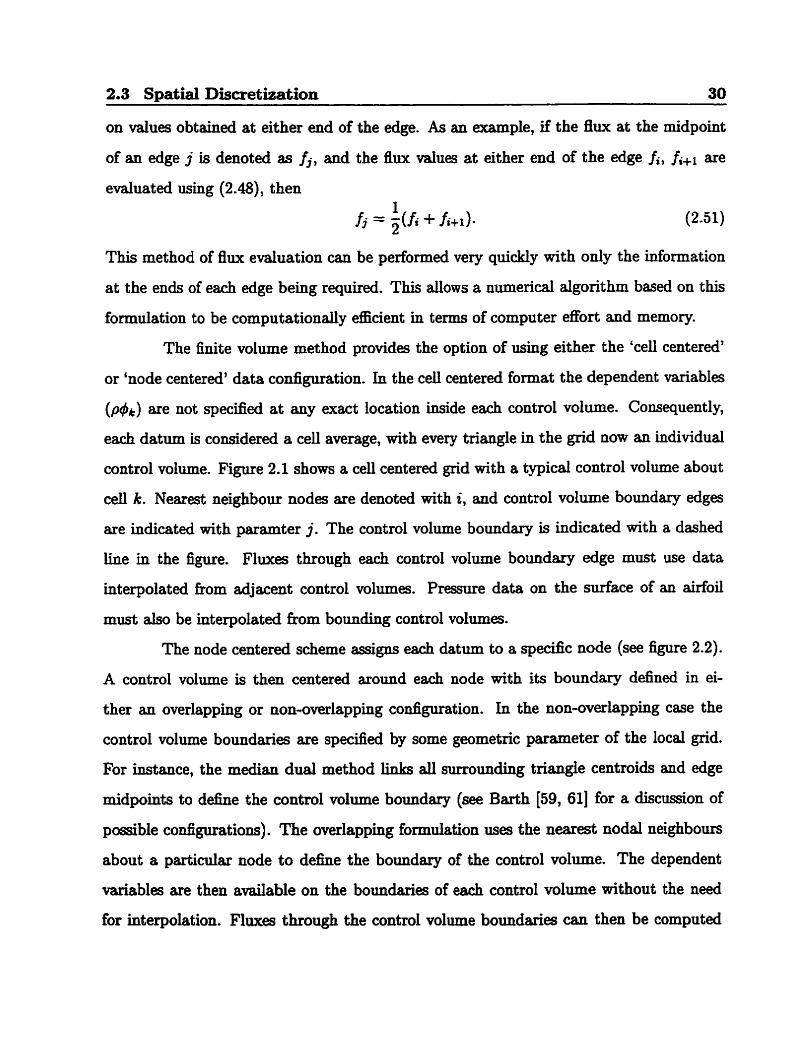
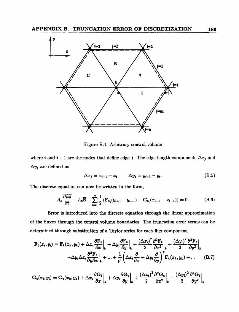
Arbitrary control volume about a central node k, with neighbour nodes i

fiom 1 to n, and boundary edges j numbered 1 to m . . . . . . . . . . . . 70 Typical stretched control volume with stretching vector and reference angle

6 i - - . . . . . . . . . . . . . . . . . . . . . . . . . . . . . . . . . . . . . - - 75

Example of an irregular control volume . . . . .. . . . . . . . . . . . . . . . 77 Error imposed on an arbitrary control volume . . . . . . . . . . . . . . . . 80 Trailing edge grid of a NACA 0012 air£oil, unsmoothed, 12420 nodes . . . . 82

Pressure field produced with lower order stretched artificial dissipation,

M,=0.5,a!=O.O, Rel=50ûû . . . . . . . . . . . . . . . . . . . . . . . . 83 Pressure field produced with higher order corrected artificial dissipation,

M,=0.5,0=0.0,&~=5000 . . . . . . . . . . . . . . . . . . . . . . . . 83

The possible refinement with a twwpass adaptation . . . . . . . . . . . . . 87

The refinement of an edge creates two new triangles and three new edges. . 87

4.3 The portion of the grid forrning the airfoil boundary- A new node is to be

. . . . . . . . . . . . . . . . . . . . . . . inserted at the body edge midpoint 93

4.4 A Line normal to the boundary edge is drawn through the interior grid.

. . . . . . . . . . . . . . . . . . . . . . . . . . m m h g points of intersection 94

4.5 The new boundary node is moved to the location specined by the spline

routine. the column of nodes above it moves in conjunction . . . . . . . . . 94

4.6 The angles considered in the Minmax edge-swapping triangulation . The

broken line indicates the other possible edge configuration . . . . . . . . . . 96

4.7 A new node is introduced into a high-aspect-ratio region of the grid near

. . . . . . . . . . . . . . . . . . . . . . . . . . . . . . . . . an airfoil surface 97

4.8 The Minmax retriangulation can generate near equilaterd triangles in high-

. . . . . . . . . . . . . . . . . . . . . . aspect-ratio regions of adapted grids 98

4.9 The stretched Minmax retriangulation avoids creating near quilateral tri-

angles in high-aspect-ratio regions of adapted grids . . . . . . . . . . . . . . 98

4.10 Adapted grid, with retriangulation . . . . . . . . . . . . . . . . . . . . . . 99

. . . . . . . . . . . . . . . . . . . . . . . . 4.1 1 Adapted grid, no retriangulation 99

. . . . . . . . . . . . . . . 4.12 Adapted grid. stretched Minrnax retriangulation 100

4.13 Adapted grid, regular Minmax retriangulation showing inappropriate tri-

. . . . . . . . . . . . . . . . . . . . . angles in the high-aspect-ratio regions 100

. . . . . . . . . . . . . . . . . . . 5.1 Unadapted grid nacaa2 with 2736 nodes 109

5.2 Extrapolation of the grid independent liR for case 1. N= total number of

. . . . . . . . . . . . . . . . . . . . . . . . . . . . . . . . . . . . gridnodes 110

5.3 Extrapolation of the grid independent total drag for case 1. N= total n u -

. . . . . . . . . . . . . . . . . . . . . . . . . . . . . . . . ber of grid nodes 110

5.4 Extrapolation of the grid independent m i o n drag for case 1. N= total

. . . . . . . . . . . . . . . . . . . . . . . . . . . . . number of grid nodes 111

5.5 Extrapolation of the grid independent pressure drag for case 1. N= total

. . . . . . . . . . . . . . . . . . . . . . . . . . . . . number of grid nodes 111

5.6 Mach number field using grid nacaa2 for case 1 . . . . . . . . . . . . . . . 112

5.7 Adapted grid using Mach number as adaptation parameter. 2887 nodes . . 112

5.8 Density field using grid nacaa2 for case 1 . . . . . . . . . . . . . . . . . . . 113 5.9 Adapted grid using density as adaptation panuneter. 2884 nodes . . . . . . 113

5.10 Pressure field using grid nacaa2 for case 1 . . . . . . . . . . . . . . . . . . 114 5.11 Adapted grid using pressure as adaptation parameter. 2882 nodes . . 114

5.12 Vorticity fidd using grid nacaa2 for case 1 . . . . . . . . . . . . . . . . . . 115 5.13 Adapted grid using vorticity as adaptation parameter. 2891 nodes . 115

5.14 Cornparison of lift results using adapted and unadapted grids. N=number

. . . . . . . . . . . . . . . . . . . . . . . . . . . . . . . . . . of grid nodes 120

5.15 Comparison of total drag results using adapted and unadapted grids. N=number

. . . . . . . . . . . . . . . . . . . . . . . . . . . . . . . . . . of grid nodes 120

5.16 Cornparison of fiction drag r d t s using adapted and unadapted grids.

. . . . . . . . . . . . . . . . . . . . . . . . . . . . N=number of grid nodes 121

5.17 Cornparison of presnire drag results using adapted and unadapted grids.

. . . . . . . . . . . . . . . . . . . . . . . . . . . . N=number of grid nodes 121

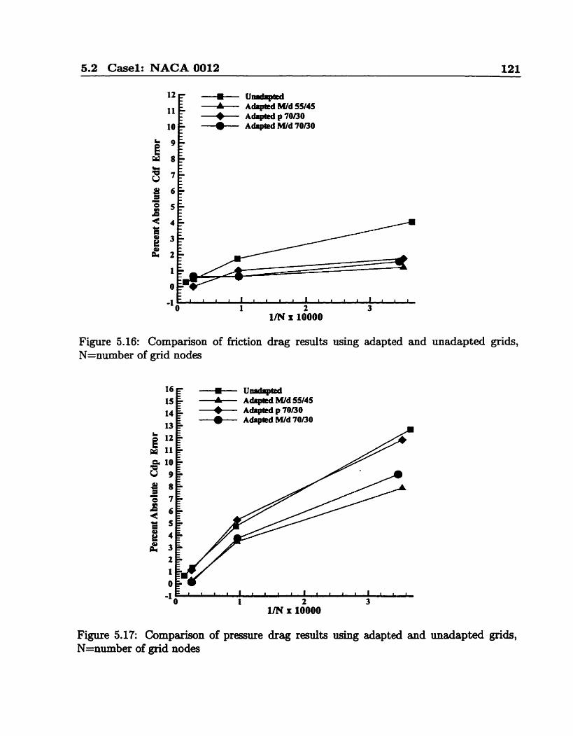
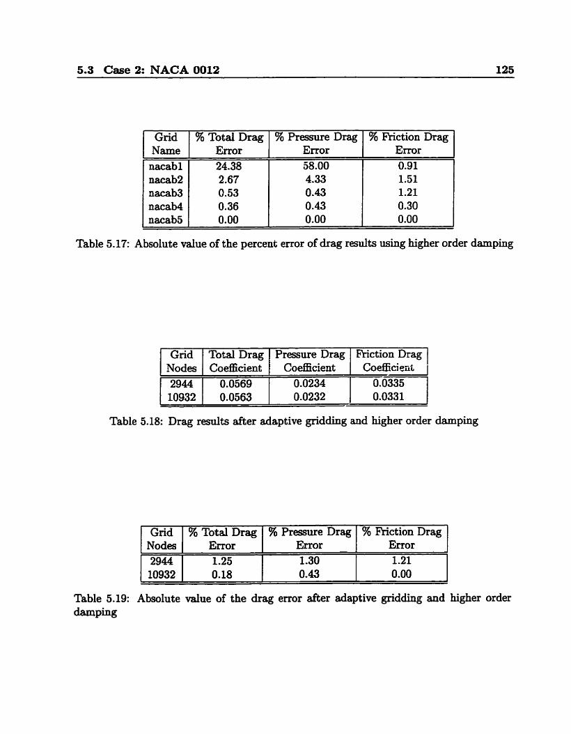
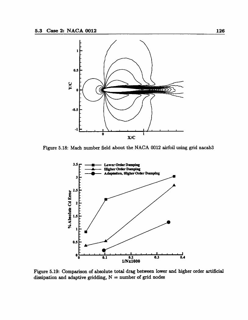
5.18 Mach number field about the NACA 0012 airfoil using grid nacab3 . . . . 126 5.19 Cornparison of absolute total drag between lower and higher order artificial

. . . . . . . dissipation and adaptive gridding. N = number of grid nodes 126

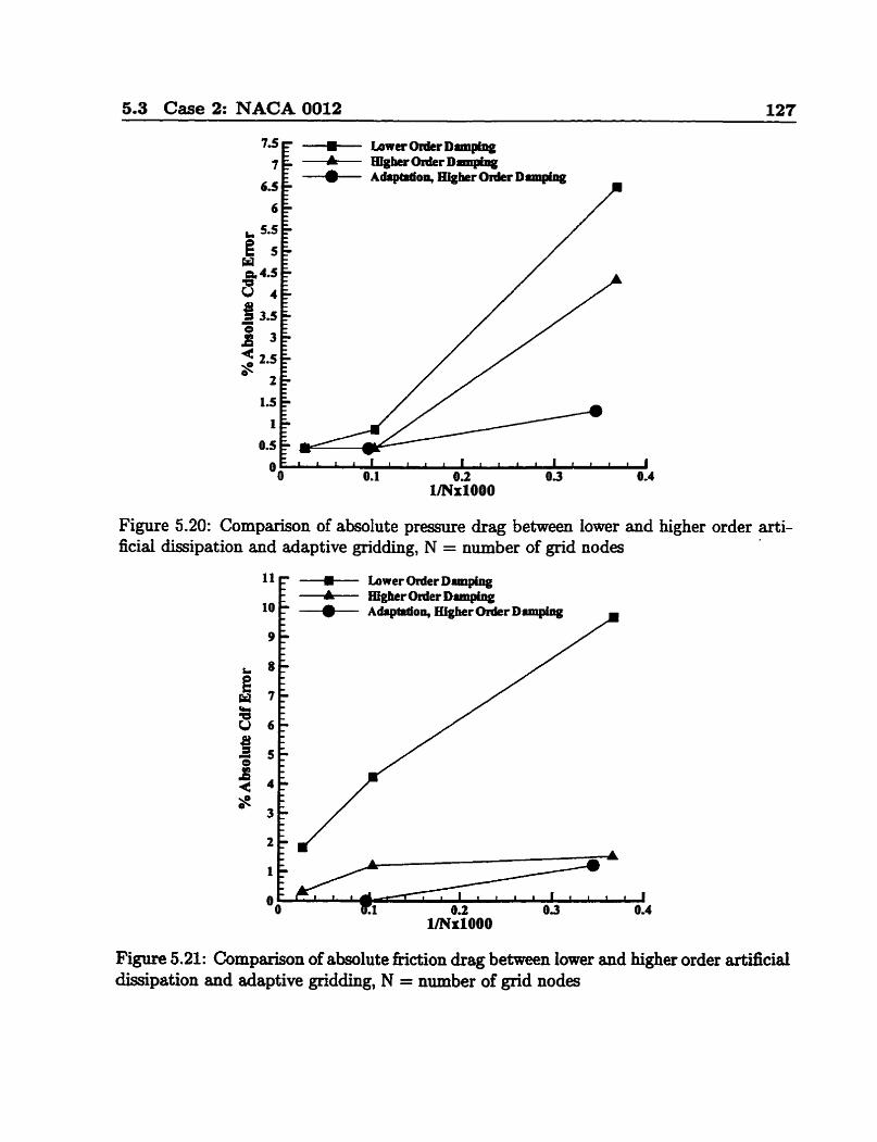
5.20 Comparison of absolute pressure drag between lower and higher order ar-

tificiai dissipation and adaptive gridding. N = number of grid nodes . . . 127 5.21 Cornparison of abso1ute fnction drag between lower and higher order arti-

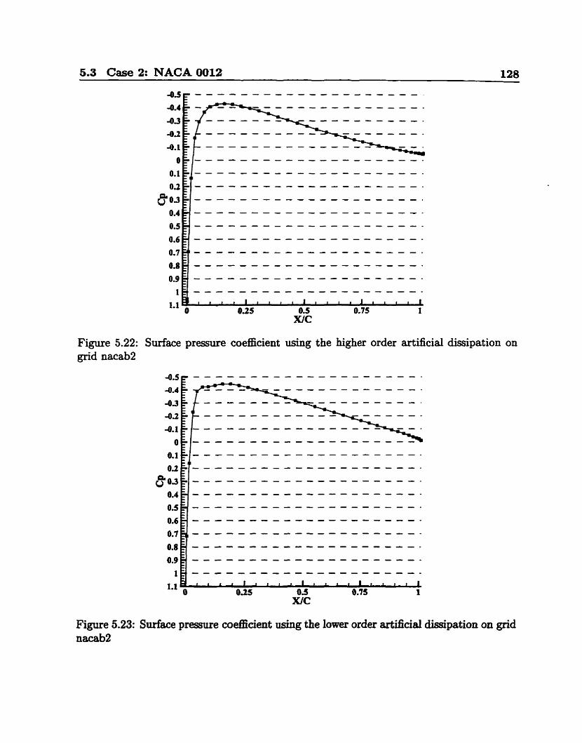
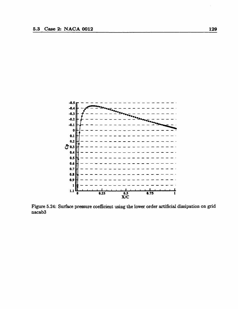
ficial dissipation and adaptive gridding. N = number of grid nodes . . . . 127 5.22 Surface pressure coefficient using the higher order artificial dissipation on

. . . . . . . . . . . . . . . . . . . . . . . . . . . . . . . . . . . grid nacab2 128

5.23 Surface pressure coefncient using the lower order artificial dissipation on

. . . . . . . . . . . . . . . . . . . . . . . . . . . . . . . . . . . grid nacab2 128

5.24 Surface pressure coefficient using the lower order artificial dissipation on

. . . . . . . . . . . . . . . . . . . . . . . . . . . . . . . . . . . grid nacab3 129

5.25 Comparison of lift coefficient produced by adapted and unadapted grids.

. . . . . . . . . . . . . . . . . . . . . . . . . . . N = number of grid nodes 133

5.26 Comparison of pressure drag coefficient produced by adapted and un-

. . . . . . . . . . . . . . . . . . adapted grids. N = number of grid nodes 134

5.27 Comparison of fiction drag coefficient produced by adapted and unadapted

. . . . . . . . . . . . . . . . . . . . . . . grids. N = number of grid nodes 134

5.28 Comparison of pressure coefficient produced by adapted grid and ARC2D 135

5.29 Comparison of pressure coeflicient produced by unadapted grid and ARC2D

135

. . . . . . . . . . . . . . . 5.30 Mach number field for the adapted grid. case 4 138

. . . . . . . . . . . . . . . . . . 5.31 Pressure field for the adapted grid. case 4 139

. . . . . . . . . . . . . . . . . . . . . . . . . . . . . . 5.32 Adapted grid. case 4 140

. . . . . . . . . . . . . . 5.33 Mach number field for the unadapted grid. case 4 141

. . . . . . . . . . . . . . . . . 5.34 Pressure field for the unadapted grid. case 4 142

. . . . . . . . . . . . . . . . . . . . . . . . . . . . 5.35 Unadapted grid. case 4 143

. . . . . . . . . . 5.36 Mach number field for the enlarged adapted grid. case 4 144

. . . . . . . . . . . . . 5.37 Pressure field for the enlarged adapted grid. case 4 145

. . . . . . . . . . . . . . . . . . . . . . . . . 5.38 Enlarged adapted grid. case 4 146

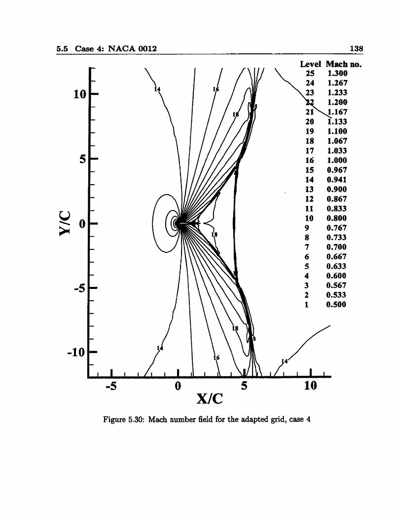
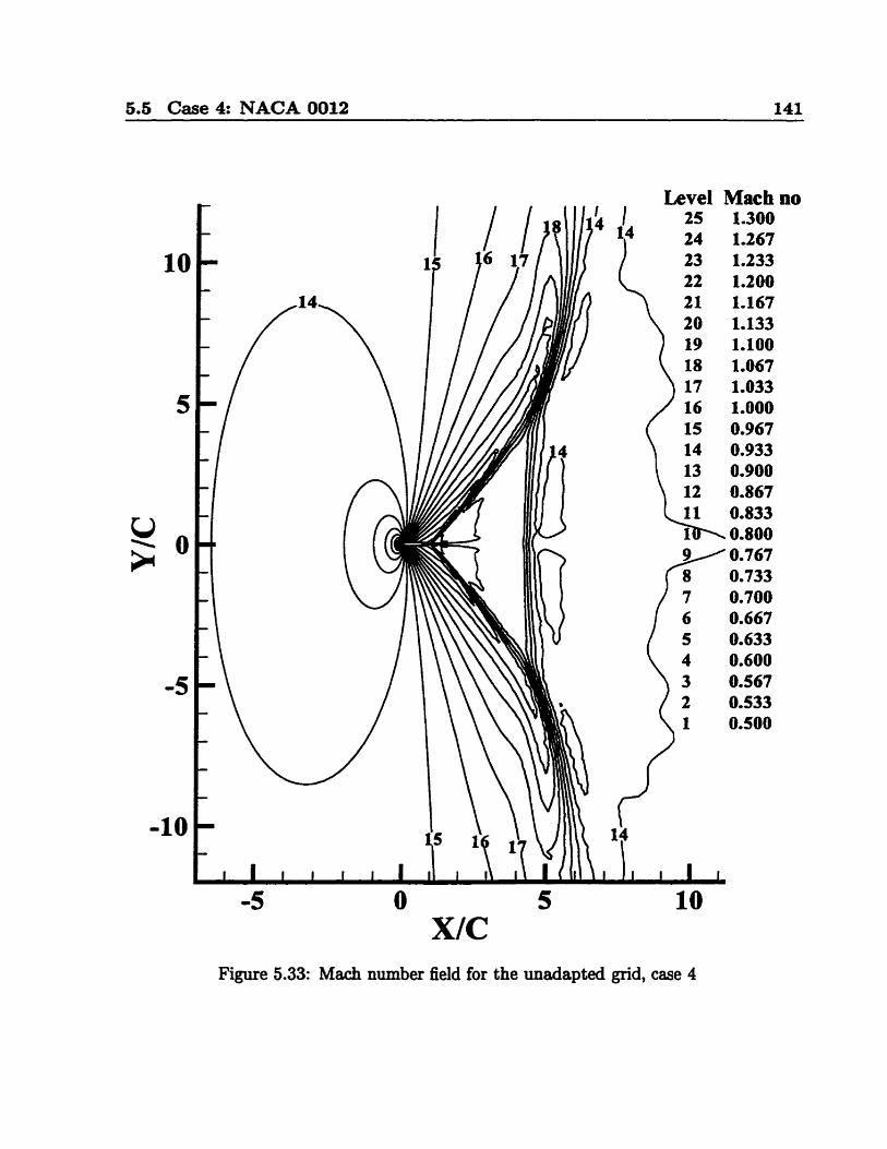
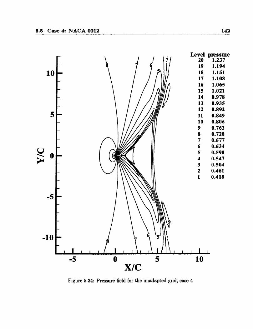
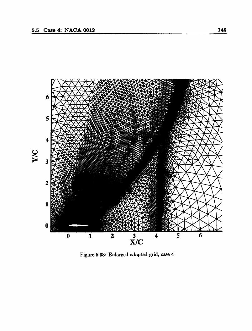
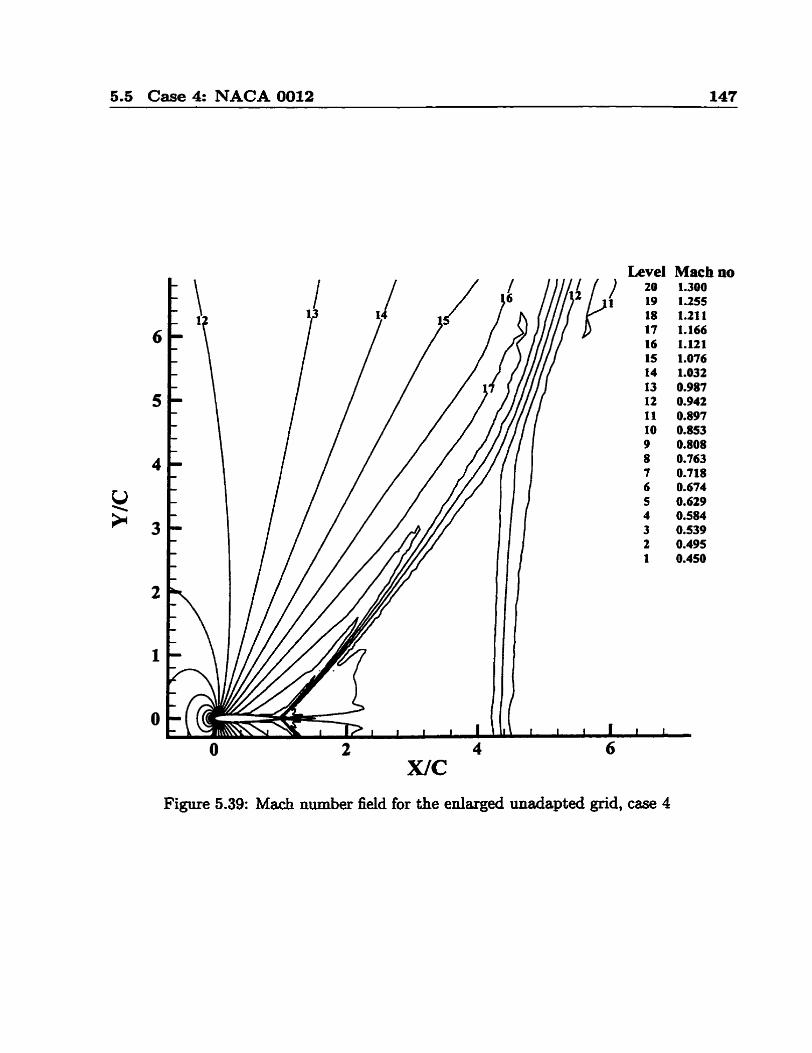
. . . . . . . . . 5.39 Mach number field for the enlargecl unadapted grid. case 4 147

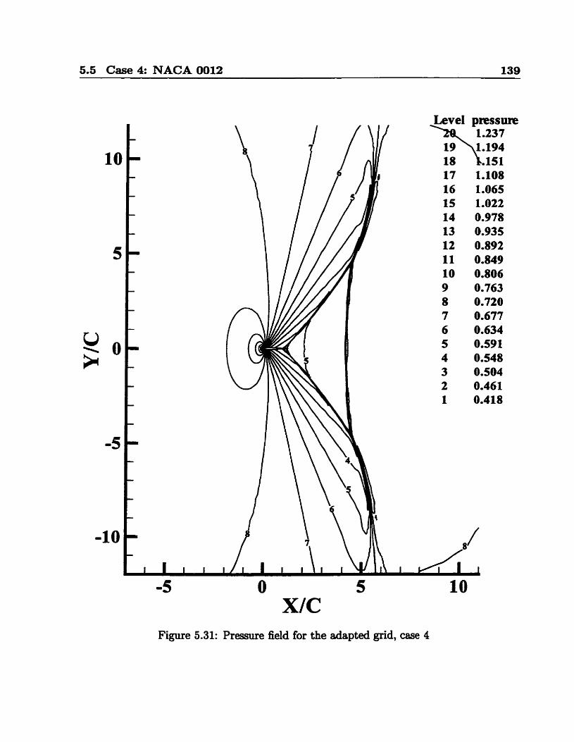
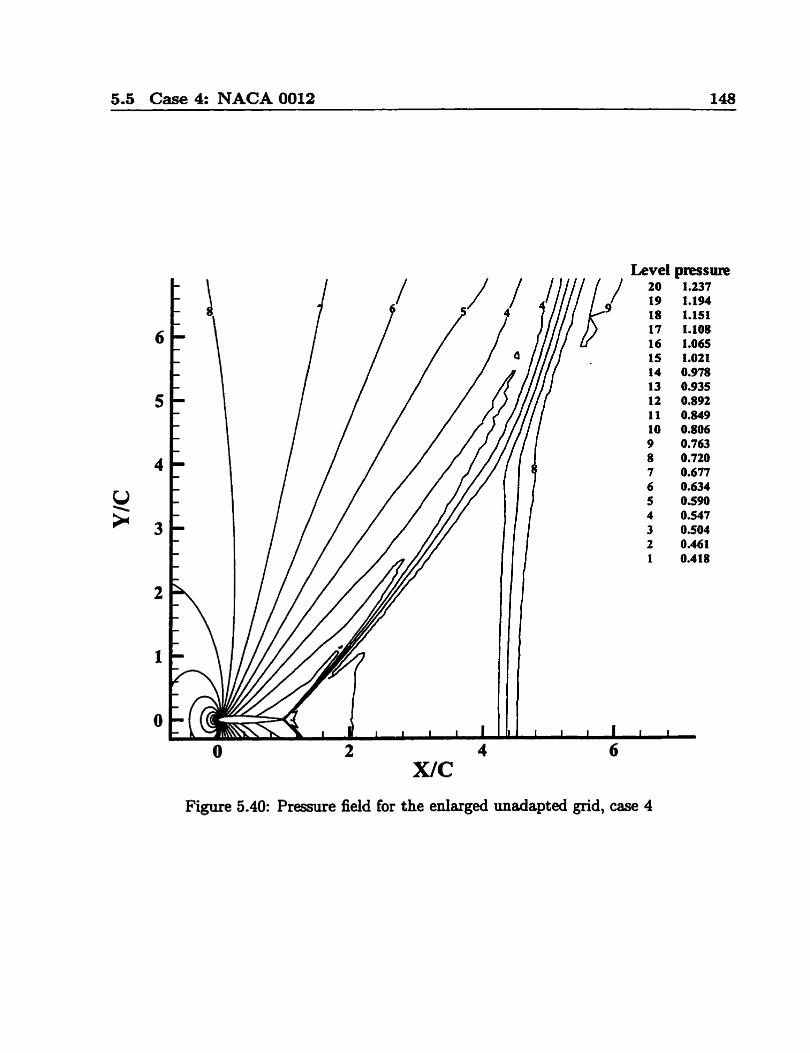
. . . . . . . . . . . . 5.40 Pressure field for the enlarged unadapteci grid. case 4 148

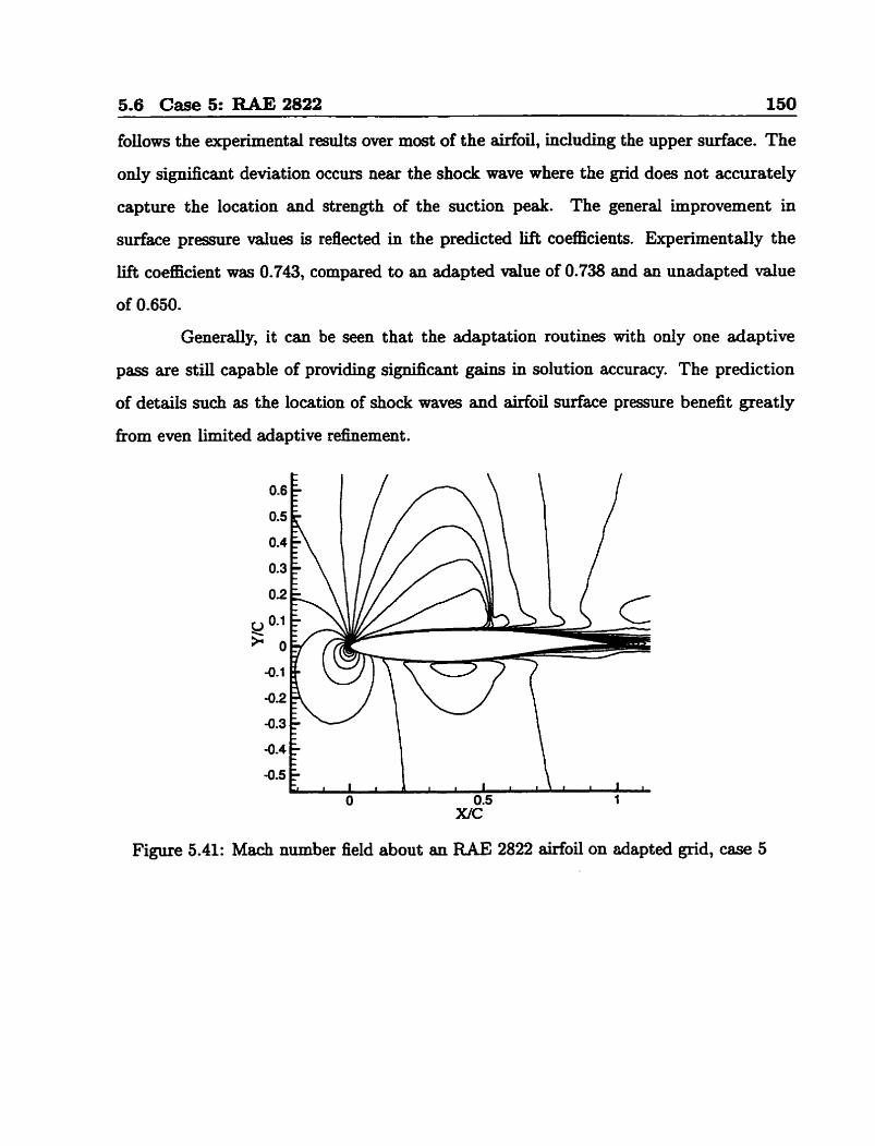
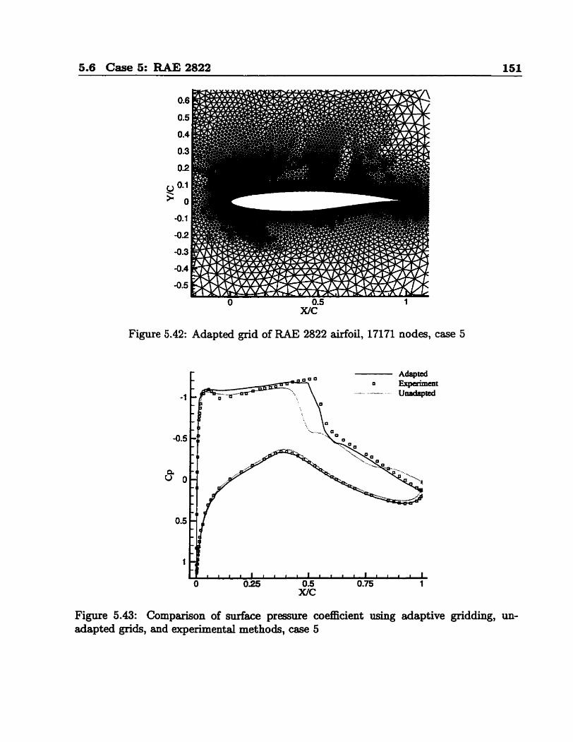
5.41 Mach number field about an RAE 2822 sirfoil on adapted grid. case 5 . . 150 5.42 Adapted grid of RAE 2822 aidoil. Inn nodes. case 5 . . . . . . . . . . . 151

5.43 Cornparison of d & c e pressure coefficient using adaptive gridding, un-

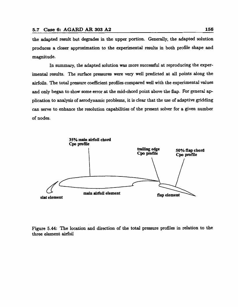
adapted grids, and experimental methods, case 5 . . . . . . . . . . . . . . 151 5.44 The location and direction of the total pressure profiles in relation to the

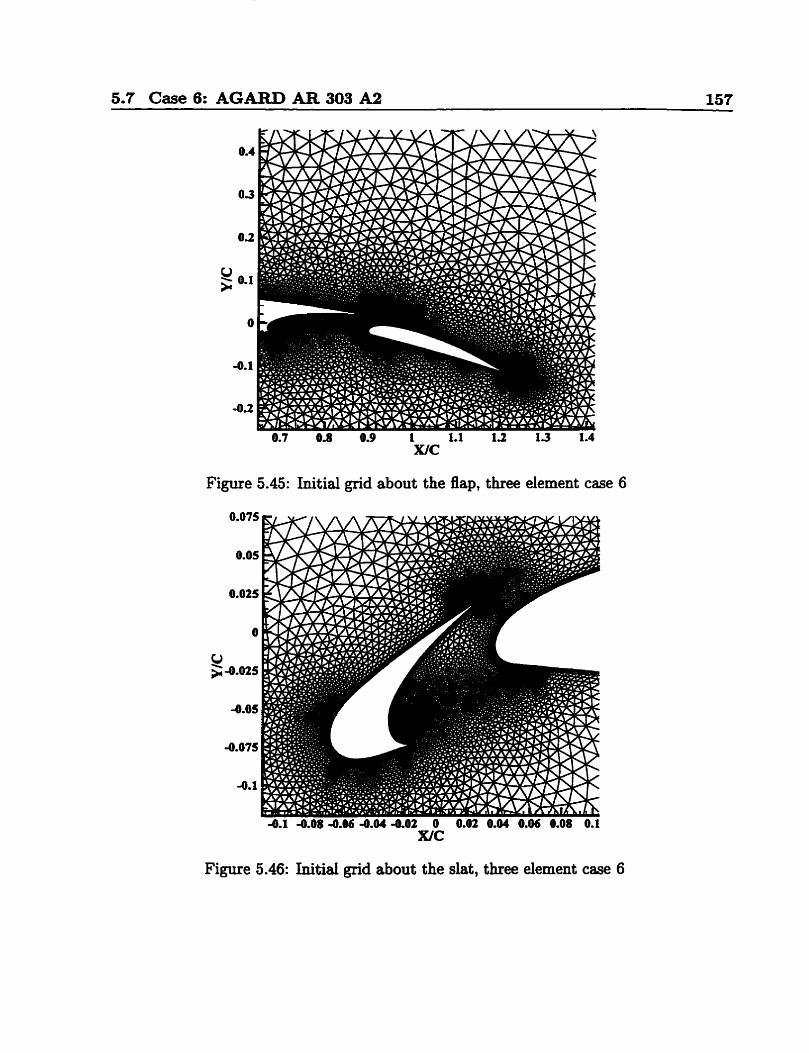
three element airfoil . . . . . . . . . . . . . . . . . . . . . . . . . . . . . . . 156 5.45 Initial grid about the flap, three element case 6 . . . . . . . . . . . . . . . 157

5.46 Initid grid about the slat, three element case 6 . . . . . . . . . . . . . . . 157

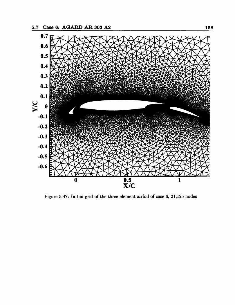
5.47 Initial grid of the three element airfoil of case 6, 21,125 nodes . . . . . . . 158

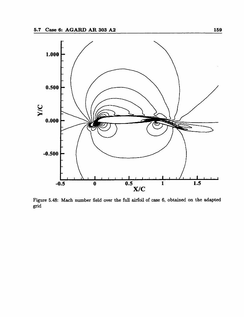
5.48 Mach number field over the fdl airfoi1 of case 6, obtained on the adapted

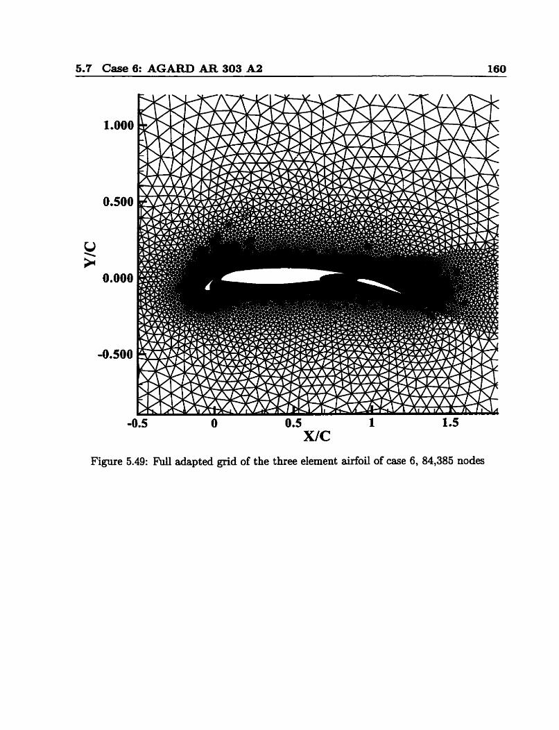
grid . . . . . . . . . . . . . . . . . . . . . . . . . . . . . . . . . . . . . . . 159 5.49 M adapted grid of the three element airfoil of case 6, 84,385 nodes . . . 160

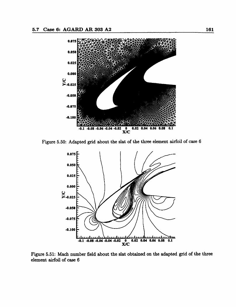
5.50 Adapted grid about the slat of the three element airfoil of case 6 . . . . . 161 5.51 Mach number field about the slat obtained on the adapted grid of the three

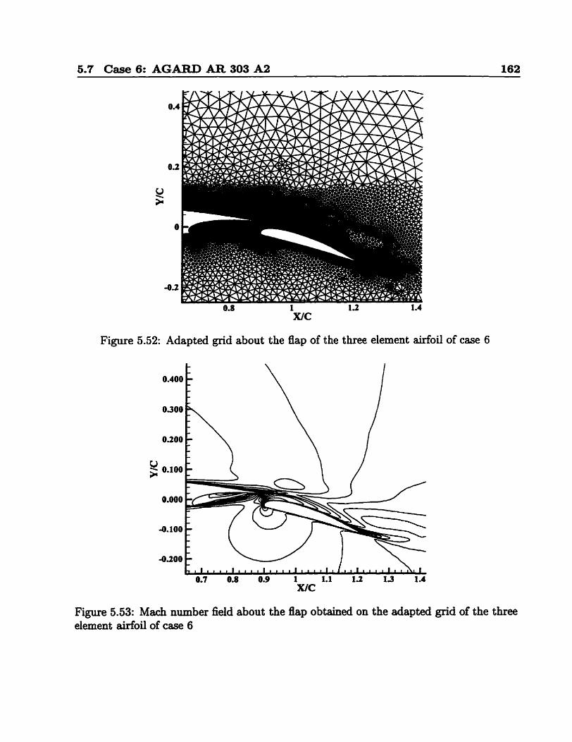
element airfoil of case 6 . . . . . . . . . . . . . . . . . . . . . . . . . . . . 161 5.52 Adapted grid about the flap of the three element airfoil of case 6 . . . . . 162 5.53 Mach number field about the flap obtained on the adapted grid of the three

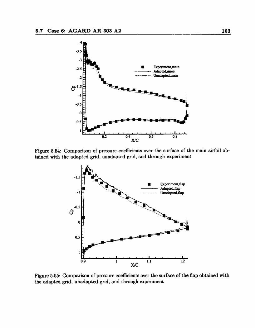
element airfoil of case 6 . . . . . . . . . . . . . . . . . . . . . . . . . . . 162 5.54 Cornparison of pressure coefficients o w the sudace of the main airfoil

obtained with the adapted grid, unadapted grid, and through experiment - 163

5.55 Comparison of pressure coefficients over the sudace of the flap obtained

with the adapted grid, unadapted grid, and through experiment . . .. . . . 163

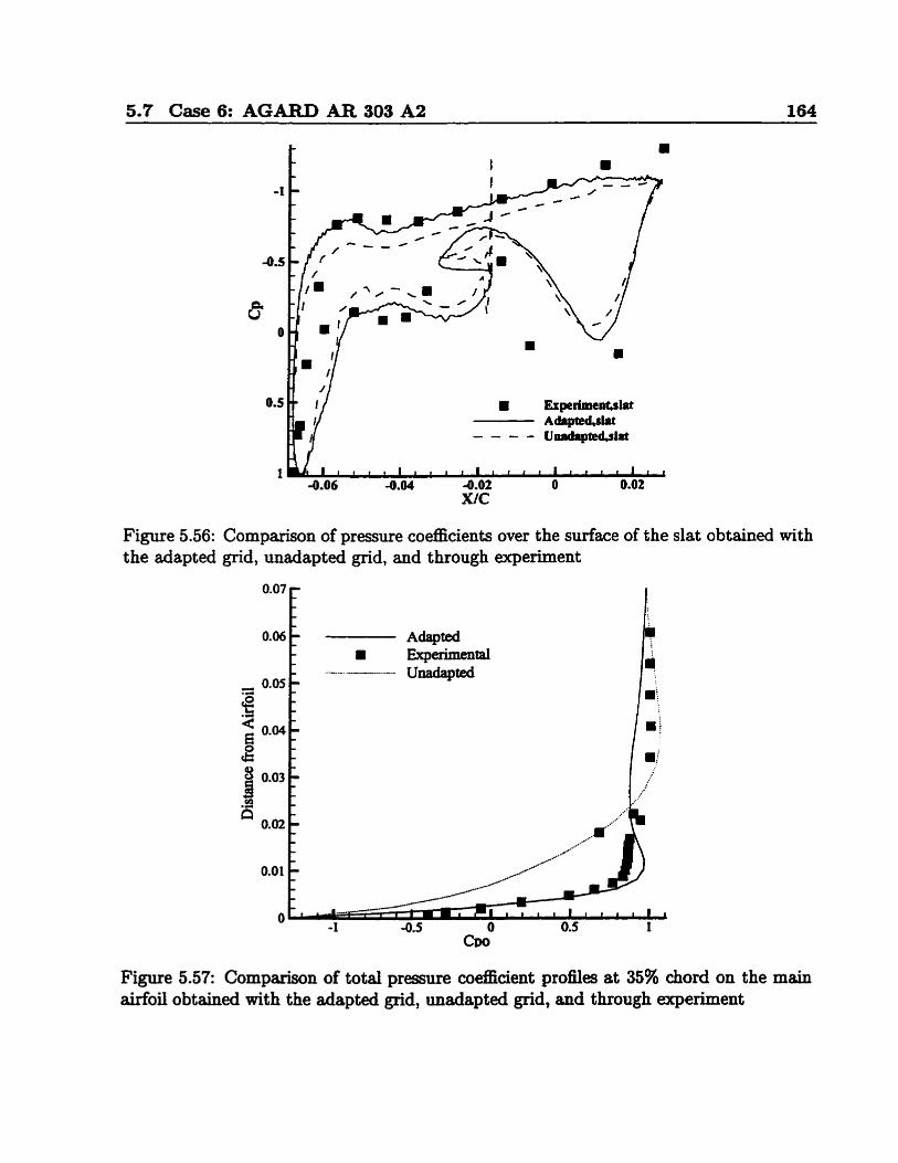
5.56 Comparison of pressure coefficients over the surface of the slat obtained

with the adapted grid, unadapted grid, and through expriment . . . . . . 164

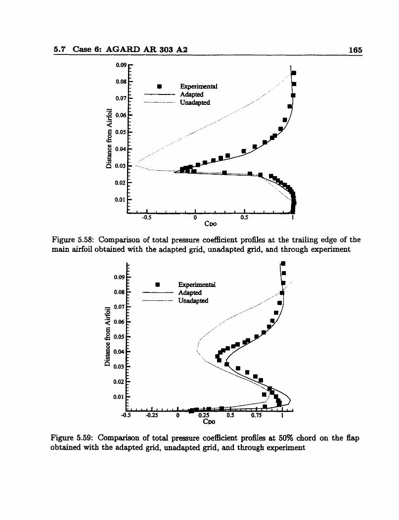
5.57 Comparison of total pressure coefficient profiles at 35% chord on the main

Mail obtained with the adapted grid, anadaptecl grid, and through exper-

iment . . . . . . . . . . . . . . . . . . . . . . . . . . . . . . . . . . . . . . 164

5.58 Cornparison of total pressure coefiicient profiles at the trsiling edge of the

main airfoi1 obtained with the adapted grid, unadapted grid, and through

. . . . . . . . . . . . . . . . . . . . . . . . . . . . . . . . . . . experiment 165

5.59 Cornparison of total pressure coefficient profiles at 50% chord on the flap

obtained with the adapted grid, unadapted grid, and through experiment 165

. . . . . . . . . . . . . . . . . . . . . . . . . . . . B.l Arbitrary control volume 186

Nomenclature

area of control volume k

control volume aspect ratio

speed of sound (non-dimensional &er page 22)

far field speed of sound

axial force coefficient

normal coefficient

lift coefficient

total drag coefficient

friction drag coefficient

pressure drag coefficient

pressure coacient

total pressure coefficient

airfoil chord length

to td artincial Mpation

distance to airfoil wail

Laphcian approximation

biharmonic approximation

distance to the turbulence trip point

total energy per unit mas (non-dimensional after page 22)

h e Stream totd energy per unit mass

interna1 energy per unit mass

artificial dissipation pressure switch

artScid dissipation pressure switch

convective flux vector, x direction

total flux vector, x direction

viscous flux vector, x direction

viscous flu tem, energy equation, x cartesisian coordinate direction

general flux term

convective flux vector, y direction

total flux vector, y direction

viscous flux vector, y direction

viscous flux term, energy equation, y direction

total flux vector

free stream enthalpy

general grid spacing

tramfer coefficients for multigrid

unit vector, x direction

unit vector, y direction

thermal conductivity (non-dimensional zrfter page 22)

free stream thermal conductivrn

artificial dissipation constant

artscia1 dissipation constant

edge length

total number of nodes forming a control volume boundw

unit normal vector in x direction at airfoil body d a c e

unit normal vector in y direction at airfoii body d a c e

hx stream Mach number

total number of edges fonning a control volume boundw

forcing fiuiction for multigrid

pressure (non-climensional &er page 22)

total pressure

fkee stream pressure

I&ar Prandtl number

turbulent Prandtl number

solution vector, [p, pu, pv, pE, pi]

universal gas constant for air

Riemann invariants at the far field boundary

Reynolds number based on speed of sound (ccrlv)

Reynolds number based on free stream velocity (cU,/v)

residual for control volume k

radial distance fkom quarter chord point to a far field node

total turbulence production variable

source term vector

stretching vector for a control volume

temperature (non-dimensional after page 22)

*ee Stream temperature

t h e (nondimemional Bfter page 22)

total rnaxknum t h e step size

m h u m convective time step size

mBlLimum viscous time step size

cartesian coordinate direction (non-dimensional after page 22)

edge length in z coordinate direction

cartesian coordinate direction (nondimemional after page 22)

edge length in y coordiaate direction

tangentid velocity at the far field boundary

normal velocity at the far field boundary

velocity difference between the airfoil wall and the local node

velocity in the z direction (non-dimensional after page 22)

fke stream velocity in the x direction

fa. field velocity in the x direction

velocity in the y direction (non-dimensional after page 22)

fkee stream velocity in the y direction

far field velociw in the y direction

angle of attack

circulation correction

ratio of constant volume to constant pressure specific heats for air

boundary for the control volume about node k

grid spacing parameters for a Stnict~red grid

polar angle between the position vector and camber line

Von Karman turbulence constant

convective spectral radius

viscous spectral radius

spectral radü for stmctured grid coordinstes

kinernatic lsrminar viscosity (non-dimensional sfter page 22)

dynarnic laminar viscosity (non-dimensional after page 22)

turbulent eddy viscosi~

fiee stream dynamic Iaminar viscosity

turbulence parameter

density (nonimensional after page 22)

fiee stream density

viscous shear stresses

general conservation variable

turbulence variable (Glu)

control volume about node k

relaxation factor for grid smoothing

vorticity at the turbulence trip point

Chapter 1

Introduction

Background

In the last few decades, the world has seen a revolution in technological achievement

brought about by the introduction of the compter microprocessor. Manufacturing au-

tomation and computer-aided design have becorne cornmonplace technologies in most

heavy industrial production enviroaments. The aerospace manufacturing industry has

evolved in the ssme m m e r . This fact was made apparent on June 12, 1994 when the

nrst prototype of the Boeing 777 made its maiden Eght. The aircraft had been predom-

inantly designecl and manufsctured with digital cornputers. The result of such increased

automation in the design and manufacture was a significant inprovernent in the overd

production efficiency. The t h e between conception and prototype completion had been

reduced fiom a typical 10 years to approximately five years. The Boeing 777 illustrates

the extent to which increased automation can impact design and manufacture and subse-

quent costs. Numerical analysis applied to the aerodynamic performance of aircraft f o m

an integral part of this design methodology.

Tkadïtionslly, aerodynamic snalysis of airmaft design was performed using both

theoretid and experirnental methods. The theoretical approach approitimates realistic

non-linear flow field phenornena with simplified mathematical relations. Although this

method can produce r d t s quickly with xninimal expense, it

ing cornplex fiow fatues. Experimental methods, however,

is ineffective in accomodat-

caa produce accurate data

1.1 Background 2

over a wide range of flow conditions. Scaled models of aircraft or wing sections are con-

stmcted and placed in wind t m e k with various data acquisition transducers. Results

of experimental origin have been heavily relied on for critical aerodynamic design. Al-

though potentially very accurate, wind tunnel tests are t h e consuming to construct and

require extensive resources. For an iterative design process, these constraints can become

prohibitive. With the rapid growth in microcomputing power and the development of

numerical models, the potential for an alternative design tool with a significant reduction

in operational expense while maintaining a high level of accuracy has been realized.

Unlike t heoretical methods, numerical models attempt to resolve all aspects of

the flow field including non-linear effets. AircraR or wing sections are represented in

computer memory as a group of interco~ected discrete points within the physical domain.

Numerical methods solve the conservation relations that represent the behaviour of a

0uid over a set of regions defined by those points. The conservation equations can be

represented over these regions in a discrete form suitable for digital processing using a

variety of methods. The cost effectiveness of a numericd model for aerodynamic analysis

is dependent not only on the power of the computer hardware but also on the accuracy

and efficiency of the various discretization methods. Several of these methods can offer

distinct advantages in cost and flexibility of application.

The discrete points or nodes about which the governing equations are solved

can be oriented in either a s t ~ c t ~ e d or unstmctured configuration (see figures 1.1 and

1.3). The structured grid maintains a rigid connectivity in relating nodes to thw nearest

neighbours, as seen in Figure 1.2. Al1 nodes other than those which define s boundary

will have four nearest neighbours. This co~mectivi@ is easily accommodated within the

array structure of computer data storage, leading to low memory requirements and easy

information r e d for such grids. However, for high lift airfoil configurations with multiple

airfoil bodies the dructured grid will enconter difücdties. The ~ t ~ c f u ~ e d format does

not easily conform to complex and irregular geometries. In such instances grid generation

1.1 Background 3

can be a complicated and t h e consuming process. The unstmctured grid does not have

this limitation since the connectivity is completeiy arbitrary (see Figure 1.4). Such grids

can conform to virtually any airfoil geometry easily, leading to grid generation processes

that are rapid and can be completely automated. The possibility then exïsts for the

creation of a completely coupled grid generator and solution algorithm that can model

flows about complex geometries while requiring ver- litt le user expertise.

The potential for an automated unstructured solver to produce weil resolved

solutions is enhanced through a solution-adaptive gridding method. Adaptive gridding

recognizes that the effectiveness of the numerid model is strongly dependent on how well

critical features of the Bow field are predicted. The presence of boundary layers, wakes,

shock waves and separated flows as well as their interactions must be accurately defined

in order to predict the lift and drag of an airfoil accurately. One possibility is the global

refinement of a grid with the knowledge that the critical features will be covered by some

parts of the fine mesh. However, since additional nodes in the simulation represent added

computational expense, using globdy fine meshes to obtain a high degree of resolution

may not be feasable. Adaptive gridding seeks to obtain the resolution of the globally

fine mesh but without the excessive numbers of nodes. Solutions on grids of moderate

resolution are initially obtained and used as the starting point for new node addition.

The solution-adaptive gridding seeks to locally refine these grids only in regions were the

solution is determined to be poorly resoIved. Thus the accuracy of the algorithm is im-

proved with fewer nodes than the global refinement. U n s t ~ ~ t ~ r e d grids are ideally suited

to adaptive gridding due to their arbitrary connectivity. New nodes cm be placed in the

grid individudy with a minimum of disniption. A structured grid requires the addition

of entire aolumns or rom of nodes to locally rehe a grid. The result is an introduction

of a large number of superfluous nodes rendering the stmctured grid impractical for node

addition adaptive gridding.

A mical example of an adapted unstmctured grid is shown in Figure 1.5. The

1.1 Background 4

Figure 1.1: Example of a structured grid

Figure 1.2: Details of structurecl grid connectivity

Figure 1.3: Example of a unstructured grid

Figure 1.4: DetaiLs of umtmctured grid comectivity

Figure 1.5: Adapted grid for NACA 0012 d o i l

Figure 1.6: Mach number field about a NACA 0012 airfoil, Mm = 0.8, a = 10.O0, Re = 500

1.2 Literature Review 7 -

influence of solution-adaptive gridding is clearly visable in the node distribution shown in

the figure. The Mach number field of the solution that lead to the creation this mesh is

presented in Figure 1.6. Through local refinement of the pertinent flow features, adapted

grids such as this are capable of producing well resolved solutions with relatively few

nodes compared to a global refmement. The development of mch unstmctured solution-

adaptive methodologies provides a means of creating an accurate aerodynamic design tool

functional over a range of flow field conditions which can be operated with minimal user

input.

Literature Review

2 1 Unstructured Solvers

The use of numerical methods as a standard design tool in the field of engineering can

trace its history back to the late 1950's. It was at this t h e that the fundamental ideas

that form the fondation of the contemporary finite element method were documented by

Greenstadt [l, 21. His theories permittecl the solution of continuous problems on a finite

set of contiguous subdomains of irreguiar shape. It was the ability of the finite element

method to resolve complex continuum problems disaetely through the unstructured na-

ture of its grids that permitted it to become an acceptecl design tool at the tirne. By the

eady 1960's the finite element method had corne into common use for structural analy-

sis in the aerospsce industry [l, 31. However, i . ~ the numerical analysis of aerodynamic

performance of aircraft the development was sornewhat slower.

In the early 1960's the fmt panel methods started to appear which permitted

the analysis of idealized flow fields about cornplex bodies [4, 51. The panel methods

assume that the 0ow field about an aerodynamic body can be approximated by a potential

function, whose behaviour can be describecl through Laplaces's equation. The simplifying

assumptions inberent to these potential solvers is that the flow field remains inviscid,

irrotational and incompressible. Panel methods detennine the appropriate distribution

1.2 Literature MW 8

of potential singularities, such as sources, sinks, and vortices, within a body such that

in a d o r m flow the streamlines codorm to the desired body shape. Tkansonic flows

can also be modeued with the linearized, s m d disturbance form of the compressible

potential equation. In 1971, Murman and Cole [6] were the first to solve the linearized

fom numerically. They used a dineremhg method that adjusted itseif to the character

of the solution. In subsonic regions of the 0ow field where the nature of the potentid

relation is elIiptic, a standard central ciifference method was adopted. However, in areas

of supersonic fiow in which the governing equation is hyperbolic, a h t order upwind

differencing method was used. The work of Murman and Cole generated considerable

activity in the field of trmsonic potential solvers and, not long after, their method was

extendecl to three dimensions [7]. Despite idealized flow assumptions, potential methods

have proven to been effective as design tools and are still in use [8]. However, some

critical aspects of realistic aerodynamic flows are characterimi by vorticity and entropy

production, and cannot be modelled with potential methods.

The inviscid Navier-Stokes equations, commonly referred to as the Euler equa-

tions, are capable of greater realisn than the potential methods. The effects of com-

pressibility can be introduced once an equation of state is specified to close the system.

Transonic flow features such as shock waves and their associated entropy production can

be modelled. Jarneson, Schmidt, and Turkel in 1981 [9] created an Euler solver that per-

mitted the independent solution of the temporal and spatial components of the system of

equations. Their algorithm solved the Euler equations on a dmctured grid using a central

dinerencing finite volume solver that achieved second order spatial accuracy on smooth

grids. Once discretized, the Euler equations were reduced to a system of ordinary Mer-

ential equations which were expLcit1y marched in time to a steady state solution using a

four step Rung+Kutta tirne march routine. Since the central merencing scheme had no

inherent damping mechsnism to control oseillatory behsviour as a solution is marched in

t h e , an artificial dissipation term was included. Jameson et al. use a term composed of

1.2 Literature Review 9

undivided dinerences of the dependent variables which approximate Laplacian and bihar-

monic operators. Switching tenns based on a LaplaQan approximation of pressure control

the emphasis of the damping term on either the Laplacian or the biharmonic component.

Shock mves require relatively heavy damping, in these regions the Laplacian damping

component is emphssized. Elsewhere, where lesser damphg is needed, the biharmonic

operator is accentuated.

The work of Jameson and Mavriplis incorporated into unstmctured triangular

solvers many of the lessons learned in the structureci solvers. In 1985 Jameson and

Mavriplis [IO] presented an algorithm that was very similar to Jarneson's 1981 solver in

that it used a central Merence finite volume scheme. However, in this work several meth-

O& of convergence acceleration originally developed on structureci solvers were adopteci.

Local time depping dowed each control volume to be marched explicitly through tirne

at its largest permissible t h e step rate. Residuals computed at each controi volume were

redistributeci to their nearest neighbours in a semi-implicit smoothing operation using

several Jacobi iterations. Residual smoothing dowed the algorithm to be rnarched in

time at more than twice the original rate. A multigrid algorithm developed by Jameson

[Il] was implemented. The method uses a series of grids of increasing coarseness to sys-

tematicdy remove erors of various fiequencies in an &&nt rnannner. Coarser meshes

were generated by strategically removing altemathg edges of a fine grid. Flow variables

and residuals computed on the h e r meshes are transferred to the next coarsest mesh

where tirne stepping is conducted. A correction factor is obtained on the coarser meshes

and is tranderred to the solution on the h e r meshes. The effediveness of the multigrid

method derives fkorn the fact that low frequency error can be removed faster with a coarse

mesh than with a very fine mesh. Jameson and Mavriplis found that they could obtain

the same accuracy and an quivalent convergence rate for the triangular grid as for an

q u i d e n t grid made of quadrilateral elements.

One drawback of this multigrid scheme is its reliance on grids that are related to

1.2 Literature Review 10 -

each other through a one-twne correspondence in the location of nodes between a fine

and coarse mesh. This precludes the possibility of adaptive gridding adding new nodes on

the hest mesh at any desired location. Jarneson and Mavriplis in 1987 [12, 131 showed

how a mdtigrid scheme could be constnicted using a sequence of progressively h e r grids

with no relation in node location. They demonstrated that this method could solve the

Euler equations on unrelated meshes as quickly as an equivalent solver h g multigrid on

a series of structureci grids.

The solution of the Euler equations on unstructured grids with the multigrid con-

vergence enhancement provides rapid analysis of many aerodynamic problems. However,

on complex problems in which the effects of viscosity have a strong influence on the so-

lution, the full Navier-Stokes equations must be solved. High lift multi-element airfoils

frequently contain some interaction between boundary layers and wakes and often create

separated boundary layer flows, all of which can only be rnodelIed through the eEects of

viscosity. One of the most significant diflEiculties with this class of problems is resolving

the boundary layer accurately. Gradients of velocity normal to an airfoi1 surface will be

severai orders of magnitude larger than those in the streamwise direction, especially for

high Reynolds number flows. To adequately resolve such features requires a high nodal

density normal to the wall relative to the streamwise density. The result is a layer of c e h

that are highly stretched, commonly known as high-aspectratio cells. Numerous works

have been conducted with the intent of soIving such problems using trianguiar unstruc-

tured meshes. Some of these include Anderson and Bonhaus [14], Barth [15], nirkel and

Swgnson [16], Peraire et al. Il?], Luo et al. [18], and Lober (191.

Much of the work done in resolving viscous flows on unstmctured grids has been

developed on solvers other than the finitevolume central difierence type. One of the

drawbacks of the central difference type methods is the insensitivity of the scalar arti-

ficiai dissipation to the various wave components of the conservation equations. In the

1980's the upwinding technique was developed that adjusted the magnitude of the dis-

1.2 Literature Review I l

sipation to each wave component. Desideri and D e ~ e u x developed one of the earli-

upwinding schemes on unstructured gnds in 1988 [201. Other algorithms used to sohe

fluid flow on unstructured grids include the finite element method, originally developed

for stress analysis. Many finite element schemes used in fluid andysis use the G a l e r h

method where the bas& and test functions are identicd [Zl]. Other established methods

include the Total Variation Diminishing (TM) scheme initiated by Harten (221, and the

Monotonie Upstream-centered Scheme for Conservation Lam (MUSCL) by Van Leer (231.

Comprehensive reviews of may unstructurecl solvers used in fluid flow analysis have been

prepared by Vdcatakrishnan [24] and by Mavriplis [25].

Work has continuecl on h i t e volume central Werencing schemes direct& to-

wards improvements in solution accuracy through enhancements to scalar artdicial dis-

sipation. In 1989 Mavriplis et al. [26] expanded on the scalar dissipation scheme that

he reported in 1985. His new method scaled the contribution of each node in the cre-

ation of the dissipation operator according to the aspect ratio and the orientation of the

l o d grid. In this manner he was able to create an artificial dissipation operator that

resembles that of sorne scalar operators on stmctured meshes that use different magni-

tudes of damping depending on the local grid aspect ratio. This new operator reduces

the magnitude of the artScid dissipation in the boundary lsyers of viscous flows reducing

solution contamination. Lindquist [27] demonstrated how an improved Laplacian opera-

tor codd be constructed by application of Gauss' theorem in the plane. Her Laplacian

formulation pennitted second order accuracy on grids formed of irregularly shaped tri-

angles. Lindquia provided several solutions of the Euler equations on transonic flow to

demonstrate improved remlution and the presemed accuracy of the scheme. Although

the improved Laplacian appraicimation produces accurate solutions on inviscid fiows, it

encounters instabiIity on stretched grids used in viscous problems. It is this difnculty

which is addressed in the higher order dissipation formulation presented in this work.


1.2.2 Turbulence Modellhg

The viscous regions about airfoils flying under realistic Eght conditions are characterized

by turbulence. Instabüities in the shear layers create turbulent fluctuations of the flow

field properties that are manifesteci through increased transport rates in these regions. If

accurate models of the fluid dynamics about aerodynamic bodies in realistic conditions

are to be achieved, the effects of turbulence must be induded. A cornmon approach to

turbulence m o d e h g is with the inclusion of an additional eddy viscosity in the conser-

vation equations. The value of the eddy viscosity is modelled through any one of a range

of methods which vary greatly in sophistication and computational expense. Algebraic

turbulence models determine the value of the eddy viscosity based on empiricism and

the local solution. Mamiplis implemented the Baldwin-Lomax [28] algebraic model on

an unstructured solver [29]. He needed to use a stmctured background grid on which to

solve the turbulence model in order to accommodate its non-local nature. It was found

that in separated regions of flow on multi-element airfoils the Baldwin-Lomax model was

unable to predict surface pressure accurately [30, 311. More cornplex turbulence models

require the solution of additional transport relations. The two-equation k - c model solves

a separate equation for both production and dissipation of turbulent kinetic energy, and

has been used widely. Two oneequation models are used frequently on unstructured

grids, the Baldwin-Barth [32] model and the Spalart-Allmaras [33] model. The Baldwin-

Barth model is a combinecl form of the k - E model. The Spalart-Allmaras model was

derived through empirical arguments, and has been shown to be effective in aerodynamic

applications [Ml.

1.2.3 Grid Generation

Before any numerical model can be used to provide a flow field andysis, a suitable grid

must be generated throughout the computational domain. The generation of unstmctured

grids has followed fiom a number of algorithm that permit a high degree of automation.

Barth [35], Mavriplis [25], and Peraire [36] have all produced reports reviewing numerous

unstructured grid generation methods, not ail of which are presented here. Unstructured

grid generation methods have usually foilowed two approaches, the advancing fiont tech-

nique or the Delaunay point insertion routines. The advancing &ont method fills a domain

by creating new triangles at the leading edge of a group of preemsting triangles (371. The

front begins with the discretized airfoil body and outer boundary, and procedes into the

computational domain. One advantage of the advancing &ont method is its ability to con-

form to the regions surroundhg complex airfoil geometries. The Delaunay point insertion

method assumes that a valid grid exists and procedes to insert new points according to

the Delaunay criterion. If a circle is dram through the three nodes at the vertices of a

triangle, the Delaunay criterion is met if no other node in the grid is within the circle.

Grid generation begins with a Delaunay grid composed of the airfoil and boundary nodes

only, and procedes with node insertion at triangle centeroids or with some other method

[38]. The high-aspect-ratio region near the Sulcfkce of an airfoi1 is often generated with the

admcing fiont method and the Steiner point insertion stratetegy [39]. The Steiner method

creates vectors rsdiating outward from the airfoi1 surfxe nodes and inserts new points

along their lengths at user s p d e d distances fkom the surface. In such grids it has been

shown by Barth [35] that the Minmax grid criterion produces smoother hi&-aspect-ratio

grids than the Delaunay method. The Minmax criterion is achieved when each edge is

orienteci in such s manner that the largest interior angle of the two triangles that share

this edge is minimixeci.

1.2.4 Solution-Adaptive Gridding

Solution-sdaptive gridding is used to irnprove the solution resolution in regions that are

determineci to contain a high degree of error. Adaptation ean be divided into three

classes, designated as r-adaptivity, h-adaptivity, and padaptiviw- In padaptation the

order of acmacy in the local discretization is increased. For a finite eiement routine this

translates to a local increase in order of the bas& function used to obtain the soliition.


In conceptual t e m the simplest adaptive method is the r-adaptive approach. In this

method, the node locations are altered to minimize a local m e m e of error. For highly

stretched grïds in high-Reynolds-number flows this could lead to diaiculties in skewness

or inappropriately srnd triangle sizes [24, 401. For compressible unstnictured flow solvers

the most commonly used adaptation method is the h-adaptive method. Here, nodes are

simply added to regions that are determined to la& refinement. A review of adaptive

methods is given in the survey paper of Powell et d. [41].

One common aspect of ad adaptive routines is their need to mesure the local

error the numerical solution in order to direct refinement. Approaches to error caku-

lation have used either a direct calculation of the truncation error or a heuristic method

using undivided differences or flow gradients. In 1985 Dannenhoffer [42] presented an

investigation of the improved performance using several undivided difference adaptation

parameters. He solved transonic inviscid flows using an embedded grid with h-adaptation

implemented in two passes. Cornparisons were made between the computation times of

adapted grids and globally rehed meshes. Adaptation was directed by undivided first and

second differences of density, pressure, velocity, and entropy. It was found that undivided

differences of density provided the greatest improvement in solution times for a given

level of solution accuracy. The adapted grids based on undivided second differences were

more irregular than the fust dinerences, and contained isolated regions of rehement. The

topologid difnculties created by the second difïerence adaptation lead to unreasonably

long nui times.

Fhrther stuclies in adaptation parameters were conducted by Warren et al. [43]

using an h-adaptive invisciid unstructured flow solver. The location of a normal shockwave

for a well known problem was used as an estimate of the solution error. Two adaptation

parameters were used to estimate the local solution error, undivided velocity dinerences

and the absolute value of the second derivatives of density. Grid edges that exceeded a

t h h o l d value of error based on the standard deviation of all edge values were flagged for

adaptation. It was found that excessive adaptation of the shock wave at the expense of

the smooth regions of flow lead to an incorrect location of the shock wave. hirthermore,

they found that improvements in the accuracy of a solution through adaptation were best

achieved when smooth regions of the flow adjacent to discontinuities were also rehed.

Other studies on error estimators were conducted using gradient measurements [44, 451.

In this instance the error indicators over shockwaves tended towards weasonably large

values as repeated refinements were conducted.

Numerous works using unstructurecl adaptive grids have been developed. Holmes

and Conne11 (461 in 1989 used a hybrid grid of quadrilateral and triangular cells for the

adaptation of a high Fkynolds number Navier-Stokes flow. The quadrilateral cells were

restricted to areas adjacent to the body and in anticipated d e regions, while triangular

cells Eüed the remaining regions. Node addition adaptive gridding was performed using

undivideci Merences of pressure and velocity dong grid &es. Holmes and Conneil

applied their algorithm successfully to attached interna1 Bows. They later extended their

algorithm to solve three-dimensional Euler flows [47].

Mavripiis applied his methodology for adaptation on t r i a n d m grids [48, 491 to

high Reynolds number serodynarnic problems in 1991 [50]. The thin boundary layers

of such flows present special problems to adaptation. The high aspect ratio of the celis

adjacent to the airfoil created a large number of cell edges located very cbse to the surface.

DifEculties c m arise in regions of cumrture when the new body node is rnoved into the

interior of the flow field where it may c r m over edges located near the body surface.

Mavripüs uses a method of edge tagging and relocation for edges above a new boundary

node that are at risk of creating c r d edges. Mavriplis also uses a modified Delaunay

retriangulation method tu realign the edges of the grid to create a smoother configuration.

Prestretching is applied to the grid according to a predetermined stretching vector before

edge mpping. This prevents the retnanguiation fkom destroying the high aspect ratio

nature of the grid in viscous regions of the flow. Stretching vectors are determined fiom

an unadapted grid before a solution is computed.

A number of methods have been developed that achieve adaptation through the

r-adaptive approach. Most such methods use a spring equilibrium method with variable

spring constants. Edges attached to each node are considerd to act in a manner equivalent

to springs, with each spring constant proportional to some m e m e of the local error or

grid quality. After several Jacobi iterations, the 'springs' wiU attain some equilibrium

state dehing the new location of the node. An edge with a high error and therefore a

high spring constant will draw the node in such a manner as to shorten the edge length

and increase the local node densi* A number of researchers have recently investigated

such methods for inviscid unstructurecl grids, such as Trepanier and Camarero (511 and

Richter and Leyland [52]. Habashi et al [53] have recently developed a finite element

solver that uses both node addition and node movement. They have applied their solver

to a number of inviscid and laminar aerodynamic problems and have successfdly shown

a global reduction in truncation error.

1.3 Objectives

The ultimate objective of this work is to construct a numerical algorithm that is capable

of accurately modelling the flow field about both single-element airfoils and cornplex

hi& lift aidoil codigurations. To be a relevant aeronautical design tool, the algorithm

must be capable of performing such calculations over a range of Reynolds numbers and

incident angles. The algorithm must therefore be sufnciently flexible in its operation to

accommodate all such demands. Such goals are embodied in the following list of objectives

which are used to guide the development of this algorithm.

1. The first objective of this work is to develop an unstructured finite-volume solver

that produces accurate solutions of redistic aemdynamic flows over two-dimensional

airfoil profiles.

1.4 Document Overview 17 --

2. The second objective of this thesis is to develop a solution-adaptive gridding scheme

using nodeaddition rehement. The procedure here is to determine which va.riables

and node allocation schernes provide the adaptive gridding scheme with the most

successful error detection as indicated by a reduction in lift and drag coefficient

error.

3. The final objective of this work is to demonstrate the effectiveness of the solution-

adaptive gridding strategy in providing well resolved solutions. Several test cases

of l h a r and turbulent airfoil flows are used to judge on both a qualitative and

quantitative basis, the improvernent in accuracy achieved through adaptation.

Document Overview

This document is divided into six chapters that cover both the details of the solution-

adaptive solver and a series of test cases used to assess its performance. The second

chapter outhes the solution of the compressible twdimensional Navier-Stokes qua-

tions through the tev volume methodology. Implementation of the turbulence model,

the t h e marching scheme, the flux integration, the boundary conditions, and the multi-

grid routine are all reviewed in this chapter. The third chapter concentrates on the

application of artficial dissipation to the solver. A traditional dissipation method and a

higher-order scheme are both presented. The higher-order method is shown to produce

srnoother solutions in the presence of irreguiar and high-aspect-ratio grids. The fowth

chapter reviews the solution-adaptive gridding method. The edge selection process and

a solution dependent retriangulation scheme are presented. Solutions to a nurnber of

aerodynamic problems for both laminar and turbulent flows are presented in Chapter 5.

Various flow field variables are investigated as possible adaptation parameters to deter-

mine the configuration that produces the lowest solution error. The adaptive gridding

scheme is shown to produce results that are more accurate than an equident unadapted

solution. Chapter 6 reviews the signifiaut features and contributions of this research and

1.4 Document Overview 18

makeç recornmendations for future work.

Chapter 2

Numerical Algorit hm

2.1 Governing Equations

The behaviour of the fluid flow about aerodynamic bodies is describecl by a coupled

set of non-linear partial differential equations collectively known as the Navier-Stokes

equations. These equations describe the conservation of mass, momentum, and total

energy of a homogeneous fluid. The simultaneous solution of these equations provides

the densi@ (p), the components of the moment- vector (pu, pu) in the x, y cartesian

coordinate directions respectively, and the total energy (pE) of the fluid. The density is

obtained through application of the conservation of mas, yielding a relation known as

the continuity equation. The mornentum components are obtained through application of

Newton's second law to yield one expression for momenturn conservation for each cartesian

component. The fmt law of thermodynarnics provides a relation to determine the total

energy of the fluid. The four goveming equations written in two-dimensional consemitive

form are given by the following expression:

where

These relations contain the laminar dynamic viscosity, denoted as p, the thermal conduc-

tivity of the fluid k, the pressure p, and the temperature T given in the Kelvin scale.

The governing relations given in equations (2.1) through (2.8) contain eight un-

known quantities (p, u, w , E, p, T , p, k). To close the system of equations four more rela-

tions are required. An equation of state can be obtEhined if the fluid medium is assumeci

to behave as a perfect gas aceording to the ided gas law, which is given as:

where R is the ideal gas constant for air. The assumption of a perfect gas allows the use

of the following thermodynmnic relations:

where e is the intemal energy of the fluid per unit maos, and Cp and C. are the specific

heats at constant pressure and constant volume respectively. The ratio of the specific heats

2.1 Goveming Equations 21

y , is assumed to have a constant value, 1.4 for air. For subsonic and transonic flows in the

absence of chernicd reaction the ratio of specik heats has negligible variation throughout

the fiow field, allowing this assumption. The total energy of the fluid per unit mass is

viewed as cornprising only of intemal and kinetic energies:

where u and v are the velocity components in the z, y cartesian coordinates respectively.

Using equations (2.10) and (2.11), the equation of state can be written in a form that

makes direct use of the solution vector Q shown in equation (2.2):

The two remaining transport properties p and k must be related to the known ther-

modynamic variables to close the system. Under subsonic and transonic aerodynamic

conditions these properties csn be considered to be dependent on the air temperature

only. Sutherland's law is used to relate the air temperature, in the Kelvin scale, to the

Here p, and T, are conditions in the fieestrearn far enough from the aerodynamic body

to negate its influence on these parameten, and are assumed to be constant. The thermal

conductivity is related to the dynamic viscosity through the Prandtl number:

In lnminm subsonic and transonic flows of air, the Prandtl number assumes a constant

value of 0.72. The Prandtl number is introduced into the total energy equation through

a change of variable in the thermal diffusivity tem. The speed of sound squared a2, is

substituted for the temperature variable based on the relation:

2.1 Governing Equations 22

The thermal diffusivity terms can be written in the foLIowing forms:

The algorithm is intended for use over a range of initial conditions and airfoil

geometries. The input parameters are the keestrearn Mach number, the laminar and tur-

bulent Prandtl numbers, and the Reynolds number based on the chord length of the airfoil

under consideration. To investigate each of these parameters independently, the governing

equations are placed in non-dimensiond form. The chord length of the airfoil, denoted

as c, and the fkeestream values of densi@ (p,), sound speed (a-), dynamic viscosity

(p-), temperature (T,), and thermal conductivity (km) are used to non-dimensionalize

the primitive variables according to:

The prime notation indicates the non-dimensional form of the variable and is omitted

fkom all subsequent variable referaces. Application of the non-dimensional format to the

governing equations yields a scaling factor:

P o o c a , Re, = Cr,

This relation is a Reynolds number based on the keestream sound speed and the chord

length. It is related to the more traditional form of the Reynolds number (Re) through

the keestream Mach number (M,):

The governing equatiom in nondimensional form now have the form:

2.2 Wbulence Modelling 23

2.2 Turbulence Modelling

It is intended that the numencd algorithm describeci in this work be applicable to re-

alistic high Reynolds number aerodynamic flows. In reality, aircraft wing sections are

used exc1usively in flow regimes that are characterized by Reynolds numbers well above

the critical value for turbulence. Such flows are defined by the fluctuations of ail the

dependent variables over a range of scales. The Navier-Stokes equations, as they have

been previously stated, are M y capable of resolving such fluctuations. Unfortunately, to

adequately resolve the length and time scales of the turbulent fluctuations would exceed

contemporary computational resowces 1541. An alternative practice is to reduce the vari-

ables into a sum of mean and fluctuating components. T i e averaging of the compressible

Navier-Stokes equations with the fluctuating components isolates the effects of turbulence

and yields the Favre form of these equations. Several additional terms proportional to

products of the fluctuating components are created. In the momentum equations, the new

terms act as additional stress terms and are commonly referred to as the Reynolds stress.

The Boussinesq approximation relates the turbulence stress terms to the mean rate of

strain through a scalar parameter referred to as the eddy viscosity. Numerous turbulence

models atternpt to determine the value of the eddy viscosity through algebraic or difFer-

ential equations. Classification of such models is ofken based on the number of additional

dinerential equations the modd introduces into the numerical environment. Models that

introduce only one additional equation are referred to as 'one equation models' and so

forth.

Recently, Godin, Nelson, and Zingg [34, 551 investigated the performance of

several one and two equations models commonly used in aerodynamic snaiysis. They

tested the Menter tw-uation mode1 and the Spalart-Aumaras and Baldwin-Barth on+

equation models on a stmctured grid solver. Test cases included single-element and

multiple-eiement high lift auf0i.k. They concluded that ad of these models performed

well based on experimentaüy determined d a c e pressures and velocity profiles. When

2.2 Turbulence Modelling 24

considering complex fiows with several confluent boundary layers and wakes the Spalart-

h a r a s model perfomed slightly better. It was &O demonstrated that for attached and

slightly separated boundary layers this model &O performed well. The Spalart-Allrnaras

is ais0 advantageous in that it requires only one additional field equation to solve, con-

serving cornputer memory and computation effort. It does not require any specific grid

structure, making it ideal for an unstructurecl algorithm.

The SpalartAharas turbulence model used in this algorithm solves a differential

expression for a turbulence parameter ü. The equation consists of convective and dinusive

components as weli as several source t e m . In conservative non-dimensional form the

dinerential expression is

+ P cb2 [ ( ~ ) ~ + ( g ) ~ ] + -- -- Re, 0 Re, (z 8s

The hemat ic eddy viscosity ut, is obtained from the following relation

where

fol = 2

2 + Gl


with the laminar bernatic viscosity u used to dehe X,

The turbulence production variable S, is dehed as the magnitude of the vorticity in the

flow field

Spalart and Allmaras use the vorticity for production based on the obsenmtion that

vorticity is present wherever turbulence exists in an aerodynamic context. The production

term (2.25) contains d, the distance to the closest waU and id, which is defined as

The destruction tenn (2.26) contains the functions

where

and

with

The function fa is defined as

Turbulence is initiateci at trip points along the airfoil d a c e at locations specified

by the user. At these points, the trip term (2.27) appearing in the turbulence mode1 attsins

sufticient value to initiate turbulence. The && of the trip term is local, meaning that

its value decreases rapidly with distance from the trip point. Tkip points are specined on


the upper and lower surfkes of each airfoil element. However, the localized nat,ure of the

trip term is such that every point near an airfoi1 d a c e will be predominantly effected

by only one trip point. The functions ftl and gt of the trip term are defined as

f t l = e t 1 gt exp (-G&[# + dg])

gt =- min 0.1, - ( ,). The distance fiom the field point to the nearest trip point is designated as 4. The

vorticity at the nearest trip point is denoted as wt. The term AU is the ciifference in

velocity between the field point and the trip, with Az being the node spacing at the

trip dong the body surface. Numerous constants are used in the mode1 which have the

following values

The Spalart-Allmaras turbulence equation is solved in the same msnner as the

general governing equation. Once resolved, the turbulence variable can be used to derive

the kinematic eddy viscosity fiom equation(2.28). Following the Favre form of the conser-

vation equations with the Boussinesq approximation the totd shear stress terms (2.42.6)

and thermal dinusvïity terms (2.16-2.17) become

2.3 Spatial Discret ization 27

Here, the dynamic eddy viscosity is denoted as b, and the turbulent Prandtl number

Prt is assigned the value 0.90 based on empincism. Traditionally, an additional term

is included in the normal stresses of the Boussinesq approximation proportional to the

turbulent kinetic energy. These terms are not present in the SpaIart-Allmaras mode1 and

are therefore not included here [33].

2.3 Spatial Discretization

The governing equations presented in the previous sections are written in a differential

format describing a continuum flow field at a discrete point. To extend the conservation

of the dependent variables to arbitrary regions of the real space domain, it is necessary

to write these relations in integral form. Considering an arbitrary control volume Qk,

integration of a generalized conservation equation yields the following expression

In this relation, C$ represents sny conservative variable on a per unit

as the z velocity component u, the y velocity component v , the total

turbulence variable Y . In the mass conservation equation the value of

mass basis, such

energy E, or the

q5 wiU be 1. The

vector H represents both convedive and diffusive fluxes for esch dependent variable.

The vector S, contains the source terms for each equation. If sources or si& of mas,

momentum, or energy e t within the flow field, the components of S will have a non-

trivial value. However, for homogeneous fluids in the a h c e of chemical reaction, such

as air in an external aerodynamic context, such influences are not present [56]. The rnass,

momentum, and energy equations will not contain source tenns. However, for turbulence

2.3 Spatial Discretkation 28

models that solve one or more conservation equations, source terms wiU be present. The

Spalart-Allmaras mode1 contains a number of terms that can be treated as source terms,

iisted in equations (2.24-2.27). If these turbulence source terms are represented by St , and

the diffusive flux terms given in equations (2.41-2.45) are used, the vectors of equation

(2.46) can be written as,

The partial derivatives of the turbulence variable in the x, y cartesian directions respec-

tively are i,,i,. The vectors fix and îi, are unit vectors in the z,y coordinate directions,

and Ft and Gt are the total flux vectors.

The integral equation (2.46) can be further simpMed such that it is more amenable

to discretization methods. The control volumes over which the integral equation is solved

are h e d in space with no movement of nodes or edges during solution. The Leibnitz

theorem [57] then allows the first term of (2.46) to be written as a function of time only.

This is a direct result of the fact that the domain of integration is not a function of time

but of space only. The divergence term can also be e x p r d in a simplifieci format.

Gauss' theorem in the plane allows the integral of the flux &vergence to be expressecl as

a line integral of the flux through the control volume boundary [58, 59, 601. This d o w s

s simplined evaluation of the convective and diffusive fluxes through the reduction of the

order of Werentiation. Uistead of calculating the spatial derivatives of the convective

fluxes, the simplifieci form only requires the dculstion of the flux components about the

outer boundary of the control volume. hpreseoting the outer boundary of the arbitrary

control volume as 6&, the integral equation (2.46) can be written as

Equation (2.49) is the starting point for the trazlsformation fkom a cornpletely analytical

problem to a discrete one. The integral terms of the equation are approximated as sum

and products of the flw terms using a process commonly referred to as discretization, thus

making them suitable for solution through numerical means. The temporal and spatial

terms can be addressed separateiy, allowing a solution process to use various combinations

of methods.

The finite volume method begins with the discretization of equation (2.49). The

dependent variables p$k in the fmt term of the equation are continuous over each control

volume. The discretization commences with the replacement of this continuous variable

with one that represents the average

fkst term can then be approximated

value over the control volume (see Figure 2.2). The

by

were dk is now the average value over the control volume. The term Ak is the area of the

control volume, which is constant and can be removed fkom the temporal differentiation.

The source term of equation (2.49) has an identical formulation to the temporal term and

can be treated in the same manner.

The second term in equation (2.49) represents the net flux through the closed

boundary of the control volume. In its present foxm, this term requires that exact ex-

pressions for the boundary fluxes be provided to complete its evaluation. Therefore, it

must also be approximated to d o w a numerical formulation. This implies that some

assumption must be made as to the representation of the flux across the control volume

boudaries. One of the most common methods is to use a trapezoidal formulation to

a p p r h a t e the integral. A linear interpolation is made of the flux h g an edge based

on values obtaineà at either end of the edge. As an example, if the flux at the midpoint

of an edge j is denoted as fi, and the flux values at either end of the edge f i , are

evaluat ed using (2.48), t hen

This method of flux evaluation can be performed very quickly with only the information

at the ends of each edge being required. This allows a numerical algorithm based on this

formulation to be computationally efficient in terms of computer effort and memory.

The finite volume method provides the option of using either the 'cell centered'

or 'node centered' data codguration. In the c d centered format the dependent variables

(p&) are not specified at any exact location inside each control volume. Consequently,

each datum is considered a cell average, with every triangle in the grid now an individual

control volume. Figure 2.1 shows a cell centered grid with a typical control volume about

cell k. Nearest neighbour nodes are denoted with i, and control volume boundary edges

are indicated with paramter j . The control volume boundary is indicated with a dashed

h e in the figure. Fluxes through each control volume boundary edge must use data

interpolated fkom adjacent control volumes. Presnve data on the surface of an airfoil

must also be interpolated from bounding control volumes.

The node centered scheme assigns each datum to a s p d c node (see figure 2.2).

A control volume is then centered around each node with its boundw defined in ei-

ther an overlapping or non-overlapping configuration. In the nonsverlapping case the

control volume boundaries are specified by some geometric parameter of the local d d .

For instance, the median dual method links all surrounding triangle centroids and edge

midpoints to d&e the control volume boundary (see Barth [59, 611 for a discussion of

possible configurations). The overlapping formulation uses the nearest nodal neighbours

about a particulaz node to define the boundary of the control volume. The dependent

vatlables are then a d a b l e on the boundaries of each control volume without the need

for interpolation. Fluxes through the control volume boundaries can then be computed

Figure 2.1: Example of a cell centered control volume about node k

directly using equation (2.5 1).

Based on its grid storage requirements and the ease of boundary flux calculations

the node centered scheme with overlapping control volumes was used in this algorithm.

Since there are a p p r h a t e l y twice as many ceh as nodes in a twdimensional unstruc-

tured grid, the ceii centered scheme will requVe additional data storage costs above that of

the node centered scheme. The non-overlapping control volume formulation sufZers from

similar difficulties. In this instance, two grids must be stored simultaneously; a primary

grid to store the nodes and their connectivity, and a secondary grid to store the control

volume boundaries. In the overlapping contml volume grid, only the primary grid will be

required for the flux dcdations (see figure 2.2). One of the primary objectives of any

numerical aemdynamic snalysis is to produce an accurate represe$ation of the conditions

on the d a c e of an airfoil. The cell centered scheme will require data extrapolations fiom

the interior of the domain to obtain airfoil d a c e pressure, density, and energy. The node

centered scheme can have nodes located on the d h c e of the airfoil negating the expense

2.3 Spatial Discretization 32

Figure 2.2: Example of a node centered control volume about node k with the control volume boundary indicated with the dashed line

and potential inaccuracy of an extrapolation of data. A comprehensive discussion of these

methods is given by Wilkinson [62], Barth [59, 611, and Swanson and Radespiel [63].

Using equations (2.50) and (2.51) the integrated conservation equation (2.49) can

be written in discrete form for a control volume centered about a node k,

The te- AZ, and Ayj are the length components of the edge j in the x and y cartesian

coordinate directions respectively. This flux term is summed over a l l m edges that form

the outer boundary of control volume k. The format of this ordinary differentid equation

permits any number of time marching stnrtegies to be applied. The five-step Runge-Kutta

method applied to the discretized equation will be reviewed in the next section.

The flues listed in equation (2.48) contain fht derivatives of the dependent

variables which must be apprcncimated at each node. FoUowhg the strategy presented

in the flux discretization, whereby Gauss' theorem in the plane was used to determine a

2.4 Teniporal Discretkation 33

control volume averaged value, the derivative evaluation can be written as,

In this expression the convention presented in figure 2.2, with the edges j forming the

boundary of the control volume numbered koom 1 to m, and the nodes i bounding the

control volume numbered 1 to n, is followed.

With the spatial discretization presented in this section, and the conservative

relations outlined in the previous section, a range of subsonic and transonic aerodynamic

problems can be attempted. The discretization att& second-order spatial accuracy

[IO, 641 on smooth grids and can be marched in time to obtain a steady-state solution.

2.4 Temporal Discretization

The previous section demonstrated a procedure for the finite volume discretization of the

advection and source terrns while neglectulg the time dependent terms. This section will

address the treatment of the time dependent terms in a manner that perxnits a solution

of the coupled set of governing equations. The objective of this numerical mode1 is to

produce a solution that is independent of any transient effects. Instead of neglecting the

transient terms of the governing equations, their presence does d o w a simple and effective

relaxation procedure in the solution of the system. The format of equation (2.52) is that

of an initial value problem on a coupled set of ordinary dinerential equations. ExpIicit

time march methods, snch as the Runge-Kutta routines, rely on the transient nature of

these equations to integrate the systern from one point in time to the next. The simplicity

and low cornputer mernory requirements of such methods highlight their effectivenets for

large problems.

The Runge-Kutta explicit time march methods have a number of advantages over

2.4 Temporal Discretkation 34

other explkit s01vers. These schemes are c l d e c i as 'one-step' methods since they ad-

vance the system in time using only the information provided in the previously computed

time step, as oppased to several previous tirne steps. This implies that the Runge-Kutta

methods need only store one additional t h e step other than the present one, reducing

the need for cornputer memory. The start up procedure is also very simple since one-step

methods need only an initial solution at t = O. A five stage Runge-Kutta scheme has been

developecl by Mavriplis [64] specincally for numerical models that rely on a multigrid rou-

tine for convergence acceleration. Multigrid routines enhance convergence through the

rapid damping of a range of error kequencies. Multigrid methods will be discussed in

greater detail in section 2.6. Mamiplis's five-stage method damps the highest error fre

quencies, which are not scted on by the multipid routine. The scheme begias with the

calculation of the fluxes and source tenns bom equation (2.52) using the dependent vari-

ables Q determined at an initial point in t h e ta. Thus, the dependent variables a t the

l outset are denoted as

by Q(3). The residual

Qb and for example at the third stage in the Runge-Kutta scheme

R over a control volume k at time step t , is defineci as,

The five stage Runge-Kutta routines cornputes the dependent variables at the new t h e

level Qb+*' using the following sequence of relaxation steps,

In these expressions, Ar is the control volume ares, At is the time step size, and D(Q)

is the artScid dissipation which is used to control numericd instabilities, and will be

discussed in detail in Chapter 3. The dissipation is calculated at the first, third, and fifth

stages only. The Runge-Kutta co&cients are defined by Mavriplis as,

Explicit time march schemes such as the five-stage Runge-Kutta have aa inherent

limit on the rate at which they can advance in tirne. This is a direct result of the limited

domain of influence prescribed by such schemes. The residuals that determine the flow

characteristics at a point are functions of the local conditions at the previously determined

t h e level Qk. Disturbances can therefore travel no faster than one local node spaeing

between updates of the solution field. This limitation is known as the Courant-F'riedrichs-

Lewy condition and for a fixed grid places a limit on the local time step size.

The speed at which a solution csn be found through the numerical mode1 can be

enhanced by advancement at the large& possible tirne step. The magnitude of the largest

time step size is determined fkom local grid characteristics and disturbance speed. In the

Navier-Stokes equations disturbances may travel through both convective and difhisive

mechanians. Any upper bound on the time step size must reflect both these Miuences.

The convedive t h e step limit Atc, and its diffusive counterpart At. can be combined to

produce a locd time step Mt,

~t = CFL ( ) Atc + At, The CFL parameter scales the time march rate by an amount specifkd by the stabüity

limits of the time march method. In this algorithm, the largest possible value of CFL

that can be used was found to be 4.

The lmgest time step size permissible is computed through the quotient of a

local grid length and the largest disturbance speed. The convective disturbance speed is

obtai~ed from the rnmchnum eigenvalue of the inviscid flux Jacobian, IU( + a, where U is

the fluid velocity and a is the local wave speed [65]. On a structured grid the convective

time step size limit in the coordinate direction 5 with local grid spacing Ac and Buid

velocity u in this direction is

The final t h e step size limit on the stmctured two-dimensional mesh would be the smd-

est of the time step &es computed fiom (2.59) in either coordinate direction. The sim-

plicity of mch a procedure is a direct result of the structured mesh having only two grid

directions that need be considered. For unstructured grids which tend to be isotropie,

order of this nature is cornpletely absent, complicating matters.

In the unstmctured mesh, the t h e step size constraints cannot be defhitively

dehed by consideration of the grid and flow field characteristics in only two coordinate

directions. A more generalized approach recognizing the arbitrary orientation of the

unstructured grid is needed. Calculating the normal flux of disturbances through the

boadaries of a control voIume k, the

matrix is dehed as

spectral radius of the convective flux Jacobian

The variables aj,uj,vj represent the linear average speed of sound and the averaged velocity

components respectively on edge j. The spectral radius in the context of equation (2.60)

is proportional to the largest possible disturbance speed integrated over a control volume

boundary. It offers a means of scaling the maximum t h e step size estimate with a

parameter that is dependent on the highest disturbance speed and independent of the

control volume orientation. The maximum convective time step size can be determined

following Mavriplis p6] and Johnston and Stolcis [60],

where Ak is the control volume area.

2.5 Boundary Conditions 37

An equident expression can be constructecl for the diffusive thne step limit.

Following the same procedure as in the convective t h e step ümit and using the maximum

eigenvalue of the diffusive operator in the Navier-Stokes equations, the diffusive time step

limit in non-dimensional temm is

A: At, = ,.

2.5 Bo-mdary Conditions

Boundary conditions must be specified at both the fsr-field boundary and at the nirfoil

surface. The manner in which these conditions are imposed and the information they

provide will determine what problem is solved. The Navier-Stokes equations contain

second-order viscous stress operators and heat flux terms. The presence of these te-

ailows not only Dirichlet boundary conditions, where specific values of the dependent

variables are imposed, but also Neumann boundary conditions where gradients of the

flow variables are specined. The following sections use both of these boundary conditions

to create realistic models of high Reynolds number steady-state aerodynamic flows.

2.5.1 Free Stream Conditions

The fiee stream flow conditions are those that would aûst if the Mail and its associ-

ated flow field disruptions were absent. Specification of these conditions is of primary

importance since they are used to set far-field boundary conditions and initial conditions.

Before the fht t h e step is taken the entire flow field is set to free Stream conditions as

an initial solution. In the next section on far-field conditions it will be apparent that ad-

justment of the flow field at the outer boundary d l require knowiedge of the free stream

conditions. Therefore, a statement concerning the derivation and d u e of the free stream

dependent variables in non-dimensional form is provided.

2.5 Boundary Conditions 38 -- - - - -- - -- - - - - - -- -- -

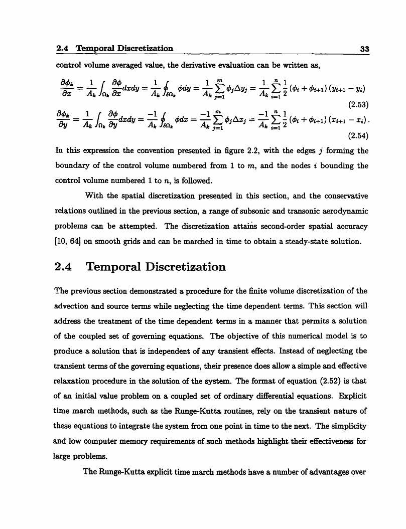
The fiee stream velocity components are determined fkom the angle of attsck

incident on the airfoil a, and the free stream Mach nurnber hioo both provideci to the

algorithm by the user.

uoo = M, cos a! v, = M, sin a. (2.64)

The pressure, density, and sound speed in the fiee stream are obtained fiom equations

(2.9,2.15,2.18,2.19) and by specifying p = p, and p = p, to yield,

Poo Poo=- - Poo - 1 -1 P m = - - - POO pooam

The kee stream total energy term is found kom equation (2.12) and the previously de-

terminecl d u e s of p,,u,,v, ,p, through,

Poo 1 E, = + -(uL + vm). - 2

The free stream total enthalpy (H,)is found fkom E,, p,, and p, using,

Pm H,=E,+-- Poo

2.5.2 Far-Field Boundary Conditions

As aircraft wings pass through the atmosphere, the aVtlow about thern is disturbed by

their presence. The domain over which this disturbance is significant c m extend a consid-

erable distance from the aidoil. Since numerical models are applied over finite regions, an

outer boundary must be placed on the computational domain. The distance of the outer

fm-field boundary fiom the aidoil and the type of boundary condition applied there can

have a significant influence on the lift and drag compnted at the aidoil surface. Pulliam

[65] conducted a numerical investigation to determine what effect the outer boundq

location had on the lift coefficient of a single element NACA 0012 airfoil. Freestream

conditions were applied at the outer boundary of a stnictured grid while the location of

the boundary was altered by successive r e m d of the outer mesh rings. This procedure

2.5 Boundarv Conditions 39 -- -- -

maintained a constant grid spacing for each case studied, dowing the effects of the outer

boundary location to be isolat&. What was shown is that the lift coefficient was adversely

affecteci by the location of the outer boundary up to the point where it was about 100

chords from the d a c e of the aidoil.

The implication of this result is that if fieestream conditions are to be imposeci a t

the outer fm-field boundary of a grid, its distance from the airfoil surface must be consid-

erable if performance characteristics are to be unaffected. Placing the far-field more than

100 chords from the airfoi1 sUTface requires either a large number of nodes in the outer

regions near the boundary or very stretched c h , both of which rnay be detrimental to

the performance of the algorithm. Additional nodes in the fax-field require greater com-

putational resources, while stretched c e h may lead to a degradation of solution accuracy.

An alternative method is to impose a correction on the far-field fiee stream conditions

in order to simulate the &ect of a larger domain had it been present. This allows the

far-field boundary to be rnoved closer to the airfoil without any l o s of accuracy. Salas et

al. [66, 671 provide a correction in the form of a velocity perturbation added to the free

stream velocities u ~ , v,. The perturbation velocities are denved assuming the effects of

the lifting airfoil can be replaced by a point vortex placed at the quarter chord location.

The circulation r induced by a point vortex is cornputed using the chord length c, and

the lift coacient Cr according to

The liR coefficient is obtained through a closeci integration of the pressure p and surface

shear stress T., about the d a c e of the airfoil. Initidy, the axial and normal force

coefficients Ca ,C, are obtained,

2.5 Boundary Conditions 40 -

where nz and n, are unit outward normal vectors in the z and y cartesian directions

respectively. The lift and drag coefficients are then determined fkom

Cd = Cn sin + Ca COS a. (2.72)

Once the lift coefficient is obtained the circulation c m be used to compute the final

far-field correc ted velocities,

The location of the nodes that define the far-field boundary are provided by their radius r

and polar angle B relative to the quarter chord point. Enforcement of constant free stream

enthalpy provides a corrected far-field sound speed which is used in the non-reflective

boundary conditions,

The solution process generates disturbances that propagate throughout the corn-

putational domain. Simple imposition of the circulation corrected fiee Stream conditions

at the far-field boundary may cause outgoing disturbances to be reflected back into the

computational domain. Non-reflective boundary conditions can be applied by consider-

ing the flow through the fa-field boundary to be l o d y one-dimensional normal to the

boundary surface. The Riemann invariants of the one-dimensionai problem are given by,

where Un is the local velocity normal to the boundary. The associateci characteristic

velocities of the Riemann invariants Ri,R2 are respectively,


The Riemann invariants are determineci through the corrected Mnables provided by equa

tions (2.73-2-75). Two additional quantities must also be specified in order to d e b e all

pertinent flow vaaiables at the boundary. These two quantities are the entropy and tan-

gential velocity Ut dehed as,

Both of these quantities are convected with the fluid flow and are therefore associated

with the normal velocity Un. The turbulence variable remains at zero on the boundary

since it is only associated with viscous effects near the airfoil surface.

Thomas and Salas [66] impose a sign convention on the characteristic boundary

conditions that determines if kee stream conditions are to be used in the calcdation of

the invariant terms or if values extrapolateci fkom the interior computational domain are

to be used instead. Fluid and disturbances moving from the interior of the computational

domain out through the far-field boundary are ansignecl a positive convention. Therefore,

at a subsonic outflow boundary node O < Un < a and X2 > O while Xi < 0, imply-

ing that invariants associated with Un and Az are defined by information interior to the

boundary. Invariants R2,R3, and & can then by determuied by values obtained fkom the

nearest interior neighbour to the boundary node in what is commonly referred to as a

'zeroth order' extrapolation. The invariant associated wit h Al, RI, represents character-

istics moving into the computational domain and must be determined from free stream

information. For a subsonic idow boundary node, -a < Un < O and invariant R2 must

again be extmpolated, whüe &,Ra, and & must now be obtained fkom the free stream.

This information is summarîzed in the following table.

2.5.3 Airfoil Surface Conditions

In viscous flow problems, such as air moving over an aidoil surfixe, the region adjment

to the airfoil inside the boundary layer will be dominated by the dects of viscosi~. The


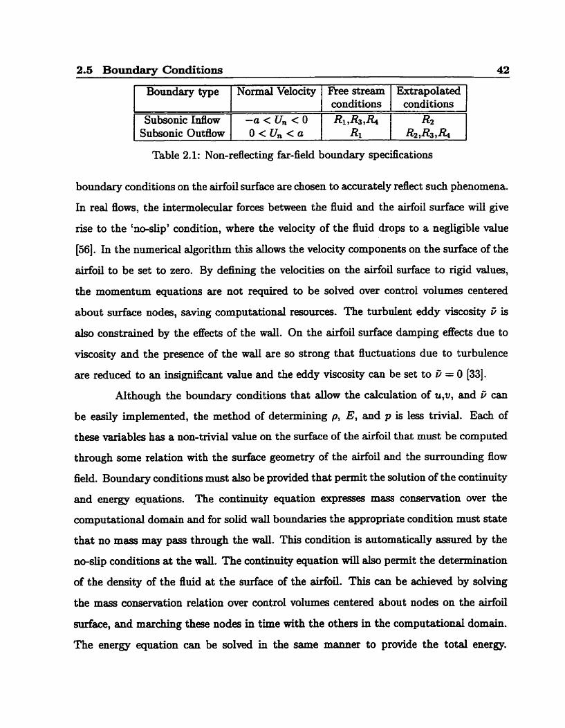
1 Boundary type 1 Normal Velocity 1 F'ree stream 1 Extrapolated 1

Table 2.1: Non-reflecting far- field boundary speciûcations

Subsonic Inflow

boundary conditions on the airfoil surface are chosen to accurately reflect such phenornena.

In real flows, the intermolecular forces between the 0uid and the airfoil surface will give

rise to the 'no-slip' condition, where the velocity of the fluid drops to a negligible d u e

[56]. In the numericd algorithm this dows the velocity components on the surface of the

airfoil to be set to zero. By defining the velocities on the airfoil surface to rigid values,

the momentum equations are not required to be solved over control volumes centered

about surface nodes, saving computational resources. The turbulent eddy viscosity B is

also constrained by the efkcts of the d. On the airfoil s d a c e damping effects due to

viscosity and the presence of the wall are so strong that fluctuations due to turbulence

are reduced to an insignScant value and the eddy viscosity can be set to 6 = O [33].

Although the boundary conditions that allow the cdculation of u,v, and i can

be easily implemented, the method of detennining p, E, and p is less trivial. Each of

these variables has a non-trivial value on the surface of the airfoil that must be computed

through some relation with the surface geometry of the ahfoi1 and the surroundhg flow

field. Boundary conditions must a h be provided that permit the solution of the continuity

and energy equations. The continuity equation expresses mass conservation over the

computational domain and for solid wall boundaries the appropriate condition must state

that no m a s may pass through the d. This condition is automaticdy assurecl by the

no-slip conditions at the d. The continuiw equation will a h permit the determination

of the demi@ of the fluid at the surface of the airfoil. This can be achieved by solving

the m a s co~~~ervation relation over control volumes centered about nodes on the airfoil

surface, and rnaxching these nodes in time with the others in the computational domain.

The energy equation can be solved in the same manner to provide the total energy.

-a < Un < O conditions

&,R3 ,& conditions

R2


However, two possibilities exist as to the themal state of the airf0i.i surface. The d a c e

termperature can be imposed by specifjhg a Dirichlet boundsry condition creating an

isothemd condition at each boundary point. The alternative is to specify the rate of

heat flux through the w d in a Neumann condition. Since the objective of this numerical

algorithm is to determine steady state solutions, the condition most consistent with the

objective is to impose an adiabatic thermal boundary condition. This condition specifies

that no thermal energy passes through the wd. It is imposed by defining the temperature

gradient normal to the d as being zero. In using the no-slip conditions, the only energy

flux that c m pass through the wall is thermal. Therefore, to impose the adiabatic wall

condition in the h i t e volume context, the heat flux terms in the energy equation along

the walls are neglected. Along waM boundaries this states

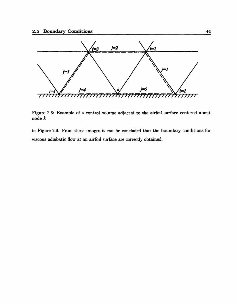
where n is the direction normal to the w d and ds is the waU edge length. Figure 2.3 shows

an example of a control volume adjacent to the airfoi1 surface. The adiabatic conditions

according to equation (2.79) will be imposed by neglecting the heat flux components

through eàges j = 4 and j = 5. Once p and E are obtained on the wd, the equation of

state (2.12) can be used to find p.

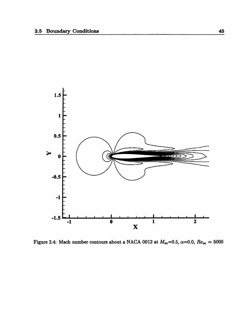
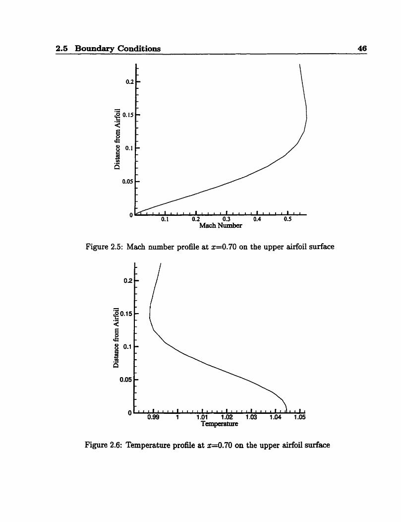
An example of the flow field near an airfoil d a c e provided by the no-slip adia-

batic boundary conditions is shown in Figures 2.4 to 2.9. The flow is about a NACA 0012

airfoil at a free stream Mach number of 0.5 et 0.0 degrees angle of attack with a Reynolds

number of 5000. Figure 2.4 shows the Mach number field about the airfoil surface. A plot

of the Mach number profde with distance from the airfoil &&ce taken at x=0.70 along

the upper surf' is given in Figure 2.5. Figures 2.6 provides the temperature profile

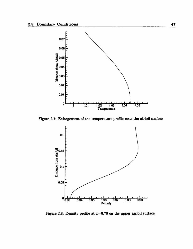
at the same point, while 2.7 gives an enlargement of this profile near the airfoil surface.

The profile dearly shows that implementation of the adiabatic boundary conditions as

describeci produces the desired zero n o d gradient at the airfoil surface. The zero nor-

mal gradient also appears in the densi@ profile in Figure 2.8 and the pressure profile


Figure 2.3: Example of a control volume adjacent to the airfoil surface centered about node k

in Figure 2.9. Rom these images it can be concluded that the boundary conditions for

viscous adiabatic flow at an aufoil surface are correctly obtained.


Figure 2.4: Mach number contours about a NACA 0012 at M,=0.5, a=O.O, R%, = 5000

2.5 Boundariv Conditions 46

Mach Number

Figure 2.5: Mach number profile at z=0.70 on the upper airfoil surface

Figure 2.6: Temperature profile at x=0.70 on the upper airfoil sudace


Figure 2.7: Enlargement of the temperature profile near the airfoil surface

Figure 2.8: Density profile at ~ 0 . 7 0 on the upper airfoil surface

2.6 Convergence Enhancement 48

9 .C

0.1 5 .d

4

B Ck

Figure 2.9: Pressure profile at z=0.70 on the upper airfoil surface

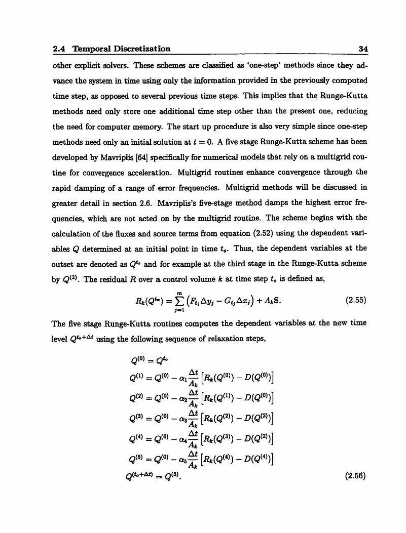
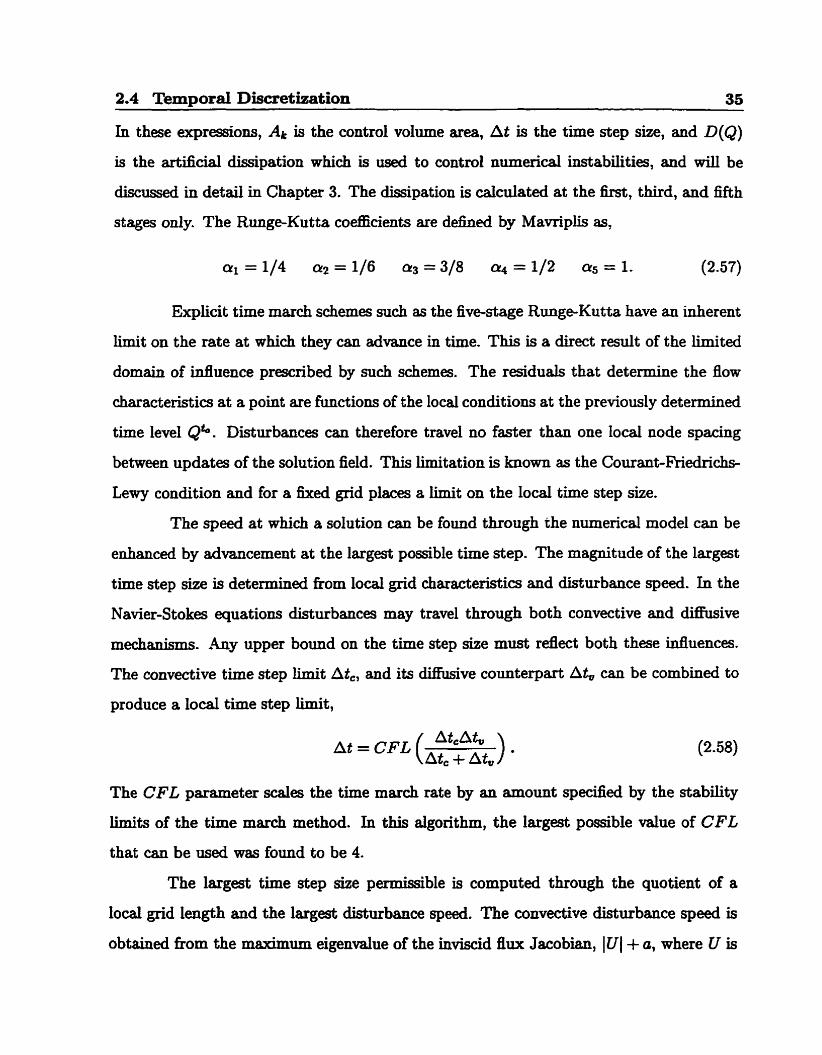
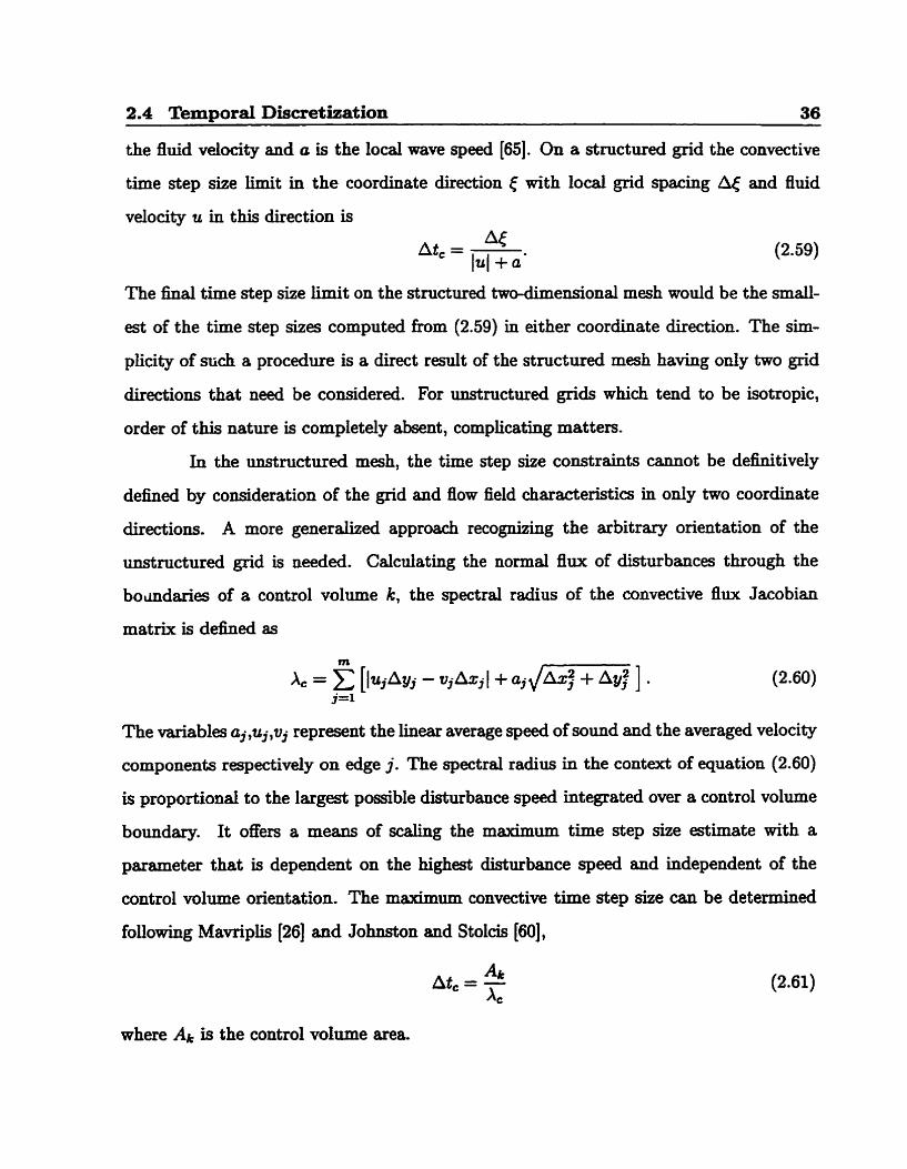
2.6 Convergence Enhancement

In section 2.4 it was seen that the explicit Runge-Kutta time m a c h method was con-

strained in the size of the largest allowable t h e step. In practical terms, information

propagating across a computational domain must do so over numerous thne steps in

order to maintain stability. For large grids with a high nodal density the amount of corn-

putation t h e to obtain a convergecl solution will be great. In cases such as high Reynolds

number flows where the off wall spacing near an airfoil body will be extremely s m d this

problem will be particularly acute. To address this diflicdm a nwnber of convergence

acceleration methods have been implemented.

2.6.1 Local Time Stepping

The maximum dowable t h e step size over an arbitrary control volume is speciiied in

equation (2.58). Each control volume will have a unique time step size limit based on the


control volume geometry and local 00w conditions. If the desireci outcome of the algorithm

was a t h e accurate evolution of a flow field, the entire computational domain must then

be advanceci at the smaüest time step found within its bounds in order to maintain a

d o m time development at each node. Since the objective of this algorithm is the

steady state solution, a uniform tirne development at each node is not required. Every

control volume is marched in time at the rate specified by its own t h e step b i t . This

permits every region of the domain to approach convergence at the maximum possible

rate based on the local grid and flow field constraints.

2.6.2 Residual Smoothing

The convergence rates of explicit tirne march schemes are restricted by the limiteci range

that disturbances may travel within a given tirne step. Increasing the distance over which

information is provided prior to any time march will permit a larger maximum time step

size. The residual smoothing method enhances the support of the algorithm by providing

each node with a residual correction based on an averaging procedure of the surroundhg

residuals [IO]. The residual used in the convergence enhancement methods is defined in

equation (2.55) with the artificial dissipation term included,

The total residual at node k is corrected based on the following implicit equation,

The total residuals designated as 'old' are the uncorrectecl values and those with 'new' are

the co~esponding corrected ones. The equation can be written in the following format,

This system of equations produces a sparse coefficient matrix which must be inverted to

cdculate &-). However, an algorithm to exactly invert this rnatrix wi l l signincantly


increase the cornputationd d o r t required for each time step. As an aitemative, restricting

the constant c to the range O < c < 1, will assure that the matrix is diagondy dominant

and the inexpensive approximate Point-Jacobi method can be used,

The residual smoothing method is applied to the newly calculated total rmidual term be-

fore t h e marchhg is conducted. The most effective configuration of the residual smooth-

h g occurs when two Point-Jacobi iterations are done, and the constant a is set to 0.175,

as determineci by Jarneson et al. [IO] and Predovic [68]. Residual smoothing was found

to approximately double the maximum time step size Limit with approxixnately a 25%

increase in computational expense.

2.6.3 The Multigrid Method

Both local time stepping and residual smoothing are effective means of enhancing conver-

gence. However, their success is limitecl by the local nature of their domain of auence .

Local time stepping influences the convergence rate of the control volume over which it

is applied. Residud smoothing uses information provided by the nearest neighbours of

a given node. Any disturbance extending over an area with a large population of nodes

will not be detected, and under such circitmstrnces the local methods will be completely

ineffective at enhmcing convergence. In this instance, only a convergence acceleration

method whose influence extends well beyond the nearest neighbours of a given node will

be effective.

The multigrid method was constructed to extend its domain of Muence to cover

the enth grid. This pefmits disturbances that extend over a large number of nodes,

oRen calied low frequency mors, to be resolved in a small number of time steps. While

this leaves the disturbances that cover only a small number of nodes, usually identifid

as high frequency error, to be reduced by the local convergence enhancement techniques.

The multigrid method recognizes the faet that mors which cover a large part of the


computational domain can best be reduced by coarse grids. The s m d nurnber of nodes

and the large tirne step sizes due to the greater node spacing allows the corne grid to

rapidly resdve such errors. Residuals and flow field information including the errors are

initidy tranderred fiom a fine mesh to a coarser one. A time step is taken on the coarse

mesh and a correction is created that is tranderred back and appüed to the fine grid.

With a series of grïds of increasing coarseness, various error fkequencies present on the

finest grid can be reduced rapidly. This is the essence of the multigrid method. On the

finest grid, high frequency errors are reduced quickly by the local convergence methods,

while the lower fiequency errors are reduced by the coarse meshes of the multigxid routine.

On a series of grids with a four-fold decrease in the number of nodes between successively

coarser meshes, the increase in cornputational efFort in multigridding is approximately

50% over the single grid solver on the hest grid per time step. However, the benefit of

this additional computational effort is an order of magnitude increase in the convergence

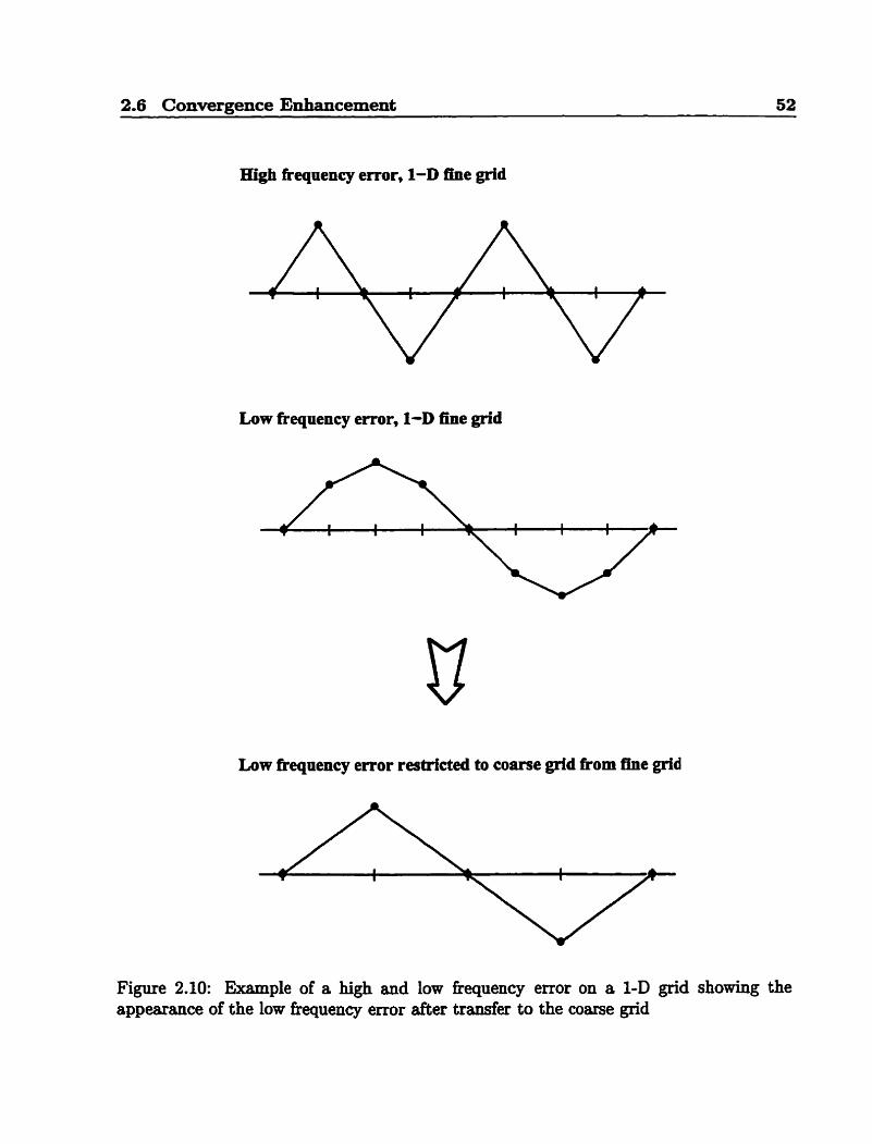
rate [64,10]. Figure 2.10 displays the appearsnce of both high and low frequency errors on

a one-dimensional grid segment. The appearance of the low frequency error after transfer

fiom the fine to the corne grid is also shown.

The full multigrid method begins with a solution obtained on the coarsest grid

of a series @ds that have a successive increase in node density. The convergence rate on

this grid is rapid due to the small number of nodes. The solution is then transferred to

the next hest grid and used as an initiai guess of the solution on this grid. The proces

of moving information fkom a coarse mesh to a finer one is referred to as 'prolongation'.

The process of prolonghg the coarse grid solution on to the fine grid is represented by

the expression

Qh = 1: Qu&* ( 2 - w

Here, Q refers to the solution vector of dependent variables Q = [p, pu, pu, pE, and

h,2h indicate the node spacing present on the grid. Thus, a grid with '2h' spacing will have

a greater distance between nodes than one with h spacing. The operator I i represents the


High frequency error, 1-D fhe grid

Low fkequency error, 1-D 5 e grid

Low fiequency error restricted to coarse grid fkom fine grid

Figure 2.10: Example of a high and low frequency error on a 1-D grid showing the appearance of the low frequency error after trader to the coarse grid


linear interpolation of information fiom the coarse grid to the finer. Once the prolongation

hom 2h to h is complete, a time step is taken on h to reduce high fiequency error. Any low

frequency error that persists is transferred back to the coarse grid dong with the solution

vector and the residuals in a process referred to as 'restriction', which is represented by

Qui = r: ~h

It should be observed that the restriction operator on the solution vector is not the

same as the operator on the residuals c. The low fiequency error is reduced quickly by

a time step on the coarser mesh.

However, since the objective of the multigrid routine is to reduce low frequency

errors on the finest grid only, the tirne step on the coarser grids should be driven by the

residuals of the finest grid. This is achieved by adding a forcing function P to the residual

on the coarse grid based on the finest grid residud,

The residual Ryi of the forcing function is computed on the coarse grid based on the

restricted fine grid solution. The forcing function is determined before any Runge-Kutta

stages are made and held fixed for the entire coarse grid time step. The Runge-Kutta

relaxation routines for stage b on the coarse grid are now,

Changes to the coarse grid solution field are a function of the fine grid residual only due to

residual cancellation of Ra in the i h t Runge-Kutta stage. In the event that the restricted

residual nom the fine grid vanishes, no changes will be made on the coarse grid solution.

If some adjustment of the coarse grid solution has been made, a correction (AQ), csn be

prolongated to the fine grid solution by


Fine Grid

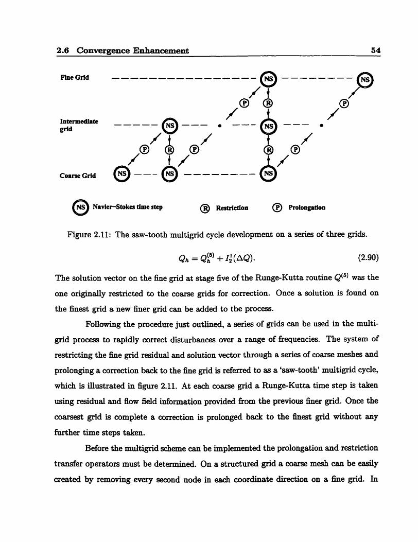
Figure 2.11: The saw-tooth mdtigrid cycle development on a series of three @ds.

Qh = ~ f ) + Ii(AQ). (2.90)

The solution vector on the fine grid at stage five of the Runge-Kutta routine Q(5) W ~ S the

one origindy restricted to the corne grids for correction. Once a solution is found on

the finest grid a new fmer grid can be added to the process.

Following the procedure just outlined, a series of grids can be used in the multi-

grid process to rapidly correct disturbances over a range of frequencies. The system of

restricting the fine grid residual and solution vector through a series of corne meshes and

prolonghg a correction back to the fine grid is referred to as a 'saw-tooth' multigrid cycle,

which is illustratecl in figure 2.11. At each coarse grid a RungeKutta t h e step is taken

using residual and flow field information provided fkom the previous ber grid. Once the

coar~est grid is complete a correction is prolonged back to the h e s t grid without any

furt her tirne steps taken.

Before the multigrid scheme can be implemented the prolongation and restriction

trander operators must be determinecl. On a structureci grid a coarse mesh can be easily

created by removing every second node in each coordinate direction on a fine grid. In


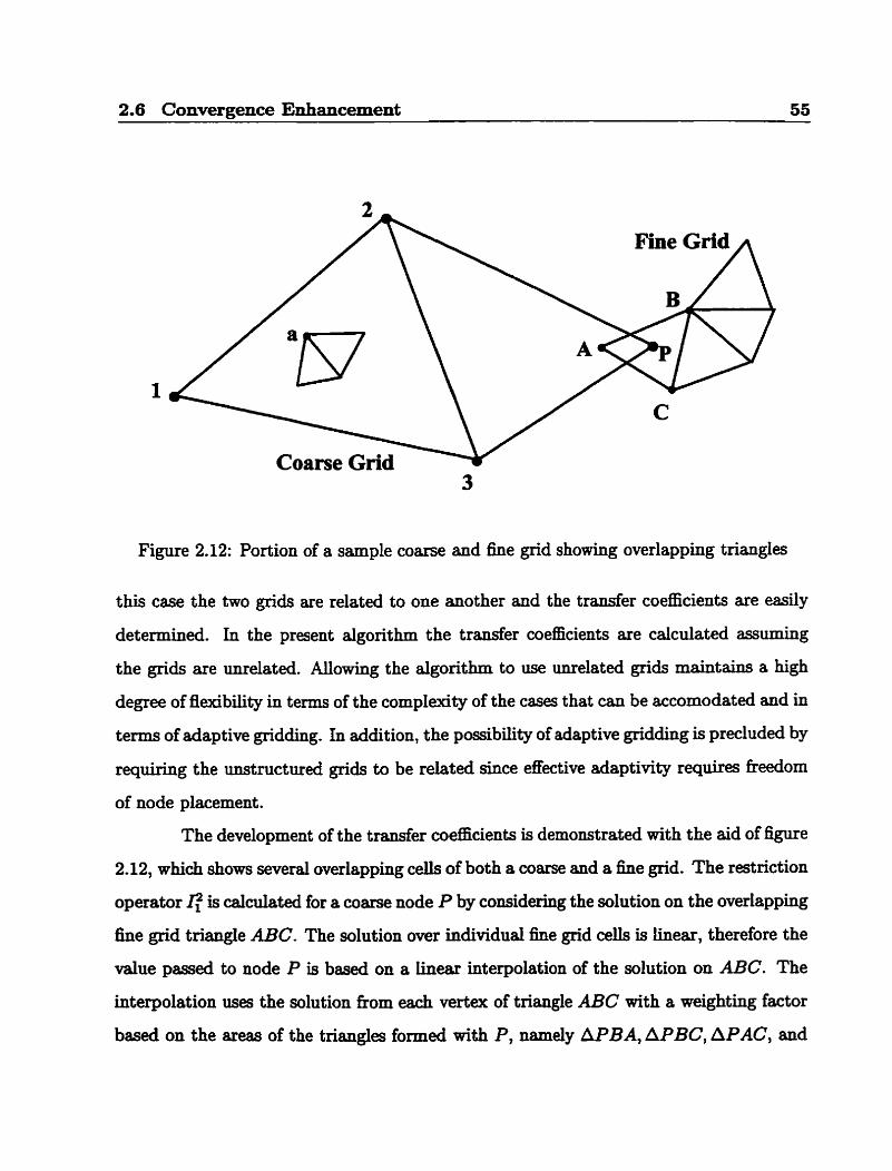
Figure 2.12: Portion of a sample coarse and fine grid showing overlapping triangles

this case the two grids are related to one another and the transfer coefficients are easily

determined. In the present algorithm the transfer coefficients are calculateci assuming

the grids are unrelatecl. Allowing the algorithm to use unrelated grids maintains a high

degree of flexibility in t e m of the complexity of the cases that can be accomodated and in

terms of adaptive gridding. In addition, the possibility of adaptive gridding is precluded by

requiring the unstructured grids to be related since effective adaptivity requires fkeedom

of node placement.

The development of the t r a d e r coefficients is demonstrated with the aid of figure

2.12, which shows several overlapping cells of both a coarse and a fme grid. The restriction

operator is calculated for a coame node P by considering the solution on the overlapping

fine grid triangle ABC. The solution over individual fine grid celle is linear, therefore the

value passecl to node P is based on a hear interpolation of the solution on ABC. The

interpolation uses the solution fiom each vertex of triangle ABC with a weighting factor

based on the areas of the triangles formed with P, namely APBA, APBC, M A C , and

2.7 Grid Generation 56

normalized with the area of ABC, M C . The value at node P is then a function of the

values at each vertex of ABC with its respective weighting factor,

APBC APAC QP = Q A - ~ +QB

APBA AABC + QcMC. (2.91)

The restriction operator that movg the fine grid residual to the coarse mesh (c) performs a dinerent function than the flow field restriction operator. The entire residual

field of the fine grid must be precisely t r d e r r e d to the came grid so that the proper

error will be reduced. AU of the residual at a fine grid node a must be distributed to

the nodes of the coarse grid triangle that encloses it (123), seen in figure 2.12. A hear

interpolation using weighting functions similar to that of the solution vector restriction

is used to distribute the fine grid residud. For the fine grid node a the residual will be

distributed according to,

The solutions and corrections that are prolonged fiom the coarse grid to a finer me&

are done so with the same operator 1'. This is accomplished using a linear interpolation

similm to that of the restriction operator. The fine grid node a is assigned the values of

the surrounding coarse grid nodes according to

The transfer coefncients are all a function of the grid geometry only. They only need

be calculateci before the solution process begins and recalled as necessary. This leads to

a computationdy efficient routine which makes multigrid a very effective convergence

enhancement method.

2.7 Grid Generation

Before any numerical flow field models can be attempted, the region about an aerodynamic

body must be reduced to a grid of control volumes over which the discretized equations


can be solved. The grid generation process is independent of, and precedes the solution

algorithm. It begins with a representation of the airfoil cross-section profile as a set of

discrete points. Profles are obtained from continuous representations of airfoil shape

through a series of spline funetions between a fked set of points [69]. The outer boundary

of the computational dornain is also represented by a series of points, which are added to

the airfoi1 data set. With both inner and outer boundaries specified the dornain can be

Wed 6 t h non-overlapping elements fiom which the control volumes can be constnicted.

The most commonly used elements to W two-dimensional cornputational domains

are triangles and quadrilatersls. The triangle is selected as the basic grid element based on

its Qmplicity and the large number of algorithms available which use it for grid generation

and postprocessing. A detailed description of a number of these methods is given by

Barth (591. Invariably these methods generate grids by trianpuiating a predetennined

set of interior points or by an advancing front method. In a given set of mesh points

a triangulation routine creates a field of non-overlapping triangles within a prescribed

geometric constraint. A triangulation that maximizes the smaLlest interior angle of a pair

of adjacent triangles that share a cornmon edge is known as a Delaunay or equilangular

triangulation. If the geometric constraint is to minimire the largest angle of the triangle

pair, the triangulation is d e d a Minmax routine. Numencal models of viscous flows

comrnonly use the Minmax routine in grid generation to avoid the possibility of creating

near quilaterd triangles in boundary layer regions that might otherwise be created with

the Delaunay method. The advancing &ont method assumes that a set of intenor points

is not a d a b l e and creates the interior grid in a series of steps. An active set of edges

forming a closed loop is definecl as the 'front'. The &ont is advancd by introducing a

new layer of points adjacent to the fiont which will serve as the new active front. With

the airfoil body and the outer boundary as the initial fronts, the entire domain is fillecl

as the imo fronts advance and ultimately rnerge.

The grid genemtion algorithm used in this numerid mode1 is a combined admc-


ing front method and Minmax triangulation. The advancing nont is used to progressively

fill the interior portions of the grid, with the Minmax triangulation used to specify the

comectivity. One of the advantages of the advancing fiont method is the ability to

specify the location of the next level of nodes according to any desired criterion. The

option is available to generate triangles that are nearly equilateral in shape or ones that

are stretched. This abiliw is critical if fi& are to be generated for use in modelling

viscous flows. The boundary layers adjacent to airfoil sUTfaces in viscous flows will con-

tain gradients in the cross-Stream direction several orders of magnitude larger than the

strearnwise direction. Efficient modelling of such flows requires high nodal density in the

cross-stream direction with sparse nodal spacing in the streamwise direction, leading to

highly stretched, high aspect ratio triangles adjacent to the airfoil surface. The advanc-

ing nont method anticipates the presence of the boundary layers by starting the node

addition process with nodes placed very near the airfoil surface. As the front moves away

fiom the airfoil, the node spacing gradually increases to the point where the triangles are

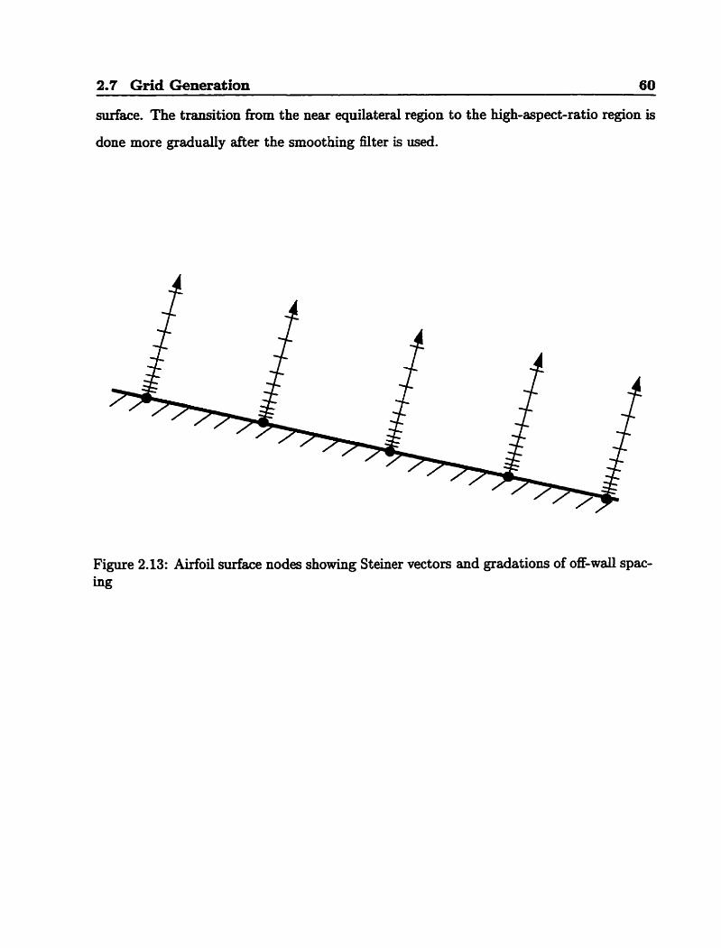
nearly equilaterd. Node placement is directed by a vector that emanates fiom the airfoil

surfsce in what is known as a stretched Steiner methodology [59]. A portion of an airfoil

surface is shown in Figure 2.13 with the direction vectors and the specified node spacing

indicated. The initial node spacing normal to the airfoil d a c e and the expansion raze

of the node spacing is set by the user prior to grid generation. Once the triangles become

nearly equilateral, the Steiner methodology is tenninated, and the advancing fkont con-

tinues with the creation of generally equilateral triangles based on the average local node

spacing dong the fiont [70].

The boundary layers on the sUTf8ce of the airfoil extend into the interior of the

computationd domain to form the wake at the traüing edge. For this reason the high-

aspect-ratio region extends downstream into the domain at the trailing edge of each airfoil

element. Figure 2.14 shows the trailing edge region of a partially completed grid. The

advancing fkont has progressed to the point where the rernaining domain is to be filled with

2.7 Grid Generation --

near equilateral triangles. Edges rdiating fiom the grid surface connect the advancing

front at the airfoil surface to the front approaching £rom the outer boundary. This is done

to ensure a smooth transition at the confluence of the two fronts. As the wake region of

the grid extends into the coniputational domain, the normal node spacing imposed at the

airfoil sudace is gradually equalized. At the end of the wake region the node spacing is

uniform, permitting a smooth transition between the hi&-aspect-ratio wake region and

the equilateral interior domain. Figure 2.15 shows the completed grid at the trailing edge.

Abrupt changes in triangle aspect ratio and control volume irregularity can cause

inflated local tnincation errors. Although every effort has been made in the construction

of the grid generation process to ensure that smooth grids are consistently produced,

some irregularity may still remain. A smoothing filter based on the undivided first-order

approximation to the Laplacian operator is applied to the x,y location of each interior

node according to

Here, the smoothing factor w is less than UXUty and n represents the number of nearest

neighbour nodes i to the central node of the control volume k. The parameter is the

control volume stretching factor, which is the ratio of the largest to the srnailest distance

fiom node k to a node i. This factor is included to prevent undesirable reductions in

normal node spacing in high-aspect-ratio regions that contain control volumes of a concave

nature. The trailing edge region of Figure 2.15 is shown after 10 sweeps of the smoothing

filter in Figure 2.16.

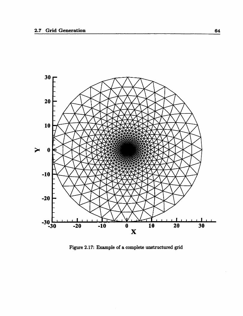
A complete grid showing both the b e r gnd and the outer boundary is presented

in Figure 2.17. This figure clearly demonstrates the disparity in node density between the

inner regions of the @d near the airfoil and the outer regions An enlargement of this

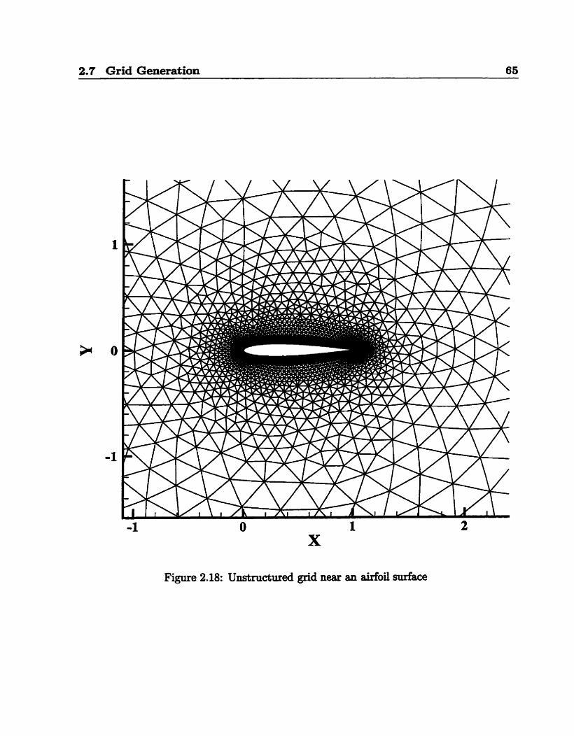
figure showing the details of the grid near the airfoil is given in Figure 2.18 . The triangles

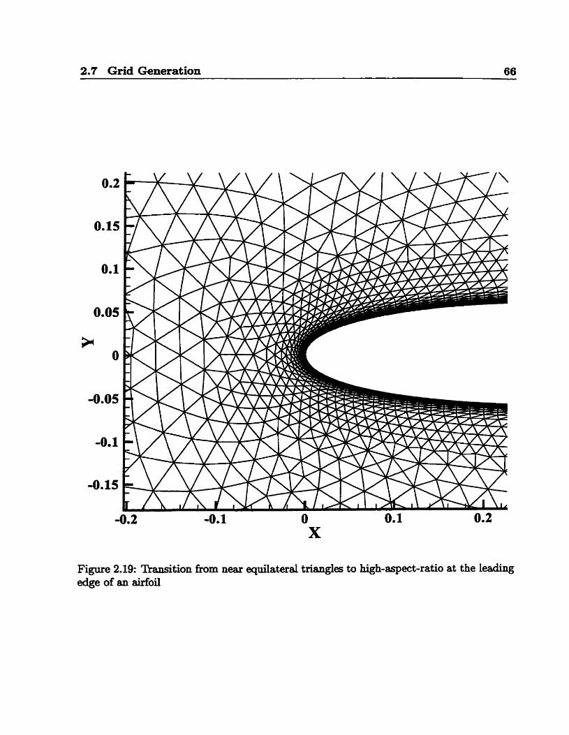
of the grid remain near equilateral over most of the computational domain. Figure 2.19

shows a further enlargement of the grid to reveal the details very close to the airfoil

surface. The transition from the near equilateral region to the high-aspect-ratio region is

done more gradually aRer the smoothhg filter is used.

Figure 2.13: Airfoi1 surface nodes showing Steiner vectors and gradations of off-wall spac-

Figure 2.14: PartialIy completed grid at the trailing edge of an aidoil showing the advancing fiont after having completed the hi&-aspect-ratio region

Figure 2.15: The complete grid near the traüing edge of an airfoil before smoothing

Figure 2.16: The complete grid near the trailing edge of an airfoil after smoothing


Figure 2.17: Exarnple of a complete unstmctured grid


Figure 2.18: UIlStTUctured grid near an aufoil surface


Figure 2.19: Thmition fiom near equilateral triangles to high-aspect-ratio at the leading edge of an Moi1

Chapter 3

Art ificial Dissipation

3.1 Motivation

The numerical algorithm outlined in the previous chapter describeci a method which com-

putes the temporal change of the dependent flow variables inside a control volume. The

value of each flow field parameter was shown to be a function of the flux through the

outer boundary of each control volume. The implications of this method is that the value

of each flow field variable is dependent on the values of its nearest nodal neighbours only,

and not on its own value. This characteristic is analogous to a central differencing approx-

imation of a fi& derivative term often used in the finite difference discretization method.

On stmctured grids central differences a p p r h a t e fi& derivatives by computing the

difference between the variables (4) on either side of a aven node and dividing by twice

the node spacing (Az),

Central Merencing achemes on uni fody spaced e d s maintain second order spatial

accuracy. This meam that the first tnincation error term of this difference method is

scaled by e, and contains the third derivatives of the field variables.

Due to the similari@ in construction, tmcation error, and stability, the finite

volume method ontlined in section 2.3 is commonly referred to as a centrd dinerencing

type fordation. The truncation error of the h i t e volume method which was used to

3.1 Motivation 68

discretize the conservation equations, is denved in Appendùc B. On smooth grids the trun-

cation error is similar to the centrai dineremhg scheme in the order of the error terms

present. Second derivative t e m are again completely absent and third derivative t e m

are the first tnuication error terms seen. Second derivative terms appear in the conser-

vation equations as difFusive phenornena, which has the effect of reducing high gradients

and dispersing any local extrema of the field variables. The absence of such damping

effects in the truncation te- leads to numerical instsbility, where s m d fluctuations in

the solution c m grow without bound as the scheme is rnarched in tirne [58]. One of the

possible instabiliw modes of an unstructured centml differencing finite volume method is

shown in Figure 3.1. Here, the values A and B represent two separate extreme values of

the field variables. The net Bux through each control volume is zero based on the linear

average of the control vohme boundary values. The field variables in each control volume

will not be altered and this osciuating field will be preserved. Additional smoothing in

the fonn of an artificial viscosity must be included to dissipate such error modes.

The purpose of artificid viscosity, or artificial dissipation as it is otherwise known,

is to simulate the error damping effécts of the d.BÛsive terms present in the consemation

equations. Once numerical stability is impsrted to the central differencing method, its sec-

ond order spatial accuracy can be used, as opposed to methods with inherent dissipation

but with lowa spatial accuracy. The diffusive effects of viscosity and thermal conductivity

create natural error damping in ail equations except the continuity equation. However,

this natural damping is confined to regions where viscous effects are well resolved and

sipnincant in value, such as in boundary layers and wakes. The majority of the computa-

tional domain is not influenced by the fluid viscosi@ and numerical instabilities remain

unchecked. An &&ive artificial dissipation method must therefore be effective over the

entire domain. The m o r mode shown in Figure 3.1 is of a high fiequency, mmeaning an

artificial dissipation scheme must also be of a local nature to control these high fkquency

components. In addition to such pmperties, an artincial dissipation method must also

3.1 Motivation 69

Figure 3.1: One error mode possible on an unstructureci grid; A and B are dinerent values of the local solution

remain dXbive with a low magnitude relative to the control volume flux. A dissipation

scheme with a large magnitude or one that introduces a convective component will not

preserve the original accuracy of the discretization method. Fhthermore, a dissipation

scheme must retain the conservative nature of the original governing equations. This is

achieved if the dissipation contribution made at a node by a neighbour i s equal in mag-

nitude and of oppusite sign to a sirnilm contribution made at a neighbouring node. In

so doing, the net flux created by the dissipation will sum to zero over the computational

domain. Not enforcing a conservative damping scheme may lead to the creation of spuri-

ous mas, momentwn, energy, or eddy viscosity. One final characteristic of concern in the

development of an artificial dissipation scheme is compntational &ciency. The dissipa-

tion parameter d l be evsluated repeatedly in the tirne marching process. Therefore, it

must be fairly simple in construction so as not to add signincantly to the computational

overhead of the complete algorithm.

3.2 Jarneson's Artificial Dissipation 70 -- - -

3.2 Jameson's Art ificial Dissipation

One of the fkst dissipation methods on unstructured grids wss proposed by Jarneson

[9, IO]. His dissipation method relies on a simple first order undividecl approximation to

the Laplacian of the field variables. The operator that he developed is easy to constmct

and accomodates the irregular nature of unstructured grids without Mculty. The Jame-

son dissipation operator is derived in a manner similar to h i t e diaerence derivations of

derivative t erms through judicious application of a two dimensional Taylor series.

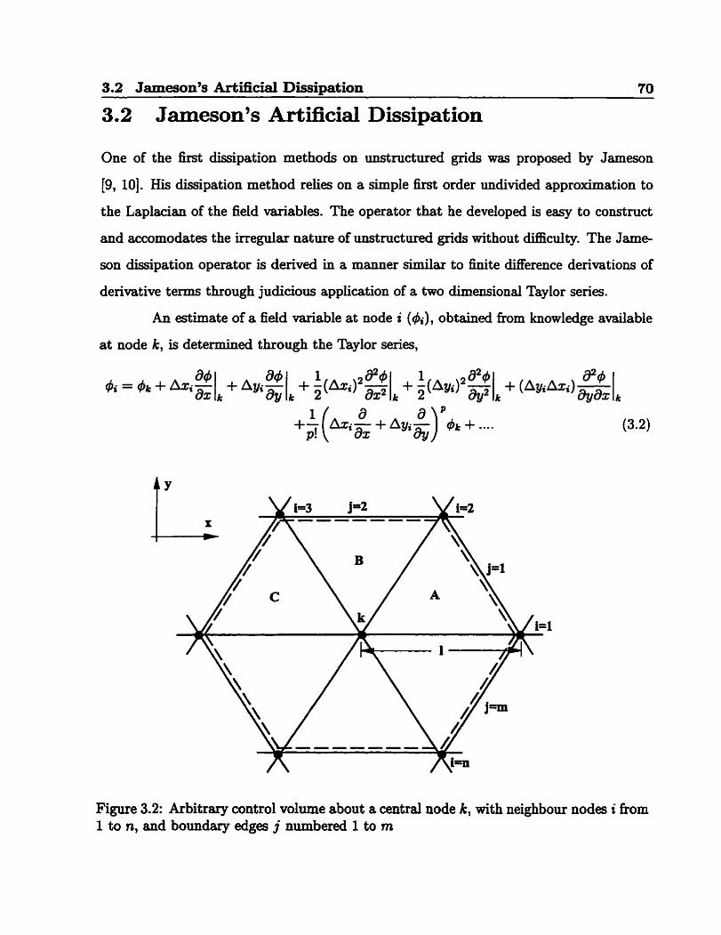
An estimate of a field variable at node i (di) , obtained nom knowledge available

at node k, is determined through the Taylor series,

Figure 3.2: Arbitrary control volume about a centrai node k, with neighbour nodes i from 1 to n, and boundary edges j numbered 1 to m

3.2 JarnesonYs ArtifkW Dissipation 71

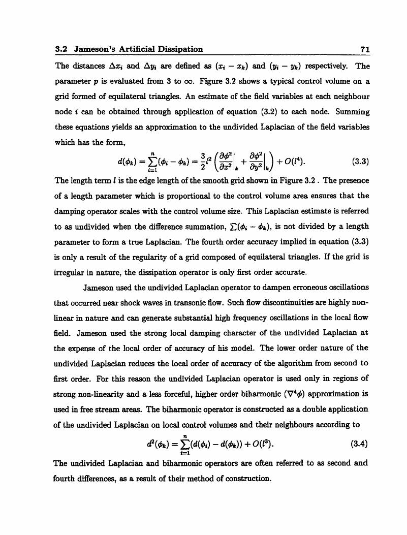
The distances hi and Agc are defhed as (xi - xk) and (yi - W) respectively. The

parameter p is evaluated h m 3 to W. Figure 3.2 shows a typical control volume on a

grid formed of equilateral triangles. An estimate of the field variables at each neighbour

node i can be obtained through application of equation (3.2) to each node. Siimming

these equations yields an approximation to the undivided Laplacian of the field variables

which has the form,

The length term 2 is the edge length of the smooth grid shown in Figure 3.2 . The presence

of a length parameter which is proportional to the control volume area ensures that the

damping operator scales with the control voLume size. This Laplacian estimate is referred

to as undivided when the dinerence summation, C(& - &), is not divided by a length

parameter to form a true Laplacian. The fourth order accuracy implied in equation (3.3)

is only a r d t of the regulari~ of a grid composed of quilateral triangles. If the grid is

irregular in nature, the dissipation operator is only first order accurate.

Jameson used the undivided Laplacian operator to dampen erroneous oscillations

that occurred near shock waves in transonic flow. Such flow discontinuities are highly non-

linear in nature and can generate substantial high frequency oscillations in the local flow

field. Jameson used the strong local darnpuig character of the undivided Laplacian at

the expense of the local order of accuacy of his model. The lower order nature of the

undivideci Laplscian reduces the local order of accuracy of the algorithm from second to

first order. For this reason the undivided Laplacian operator is used only in regions of

strong non-lineariw and a legs forceful, higher order biharmonic (V49) approximation is

used in fiee stream areas. The bihannonic operator is constructed as a double application

of the undivided Laplacian on local control volumes and theh neighbours according to

The undivided Laplacian and biharmonic operators are often referred to as second and

fourth dinerences, as a r e d t of their method of const~ction.

3.2 Jameson's Artficial Dissipation 72

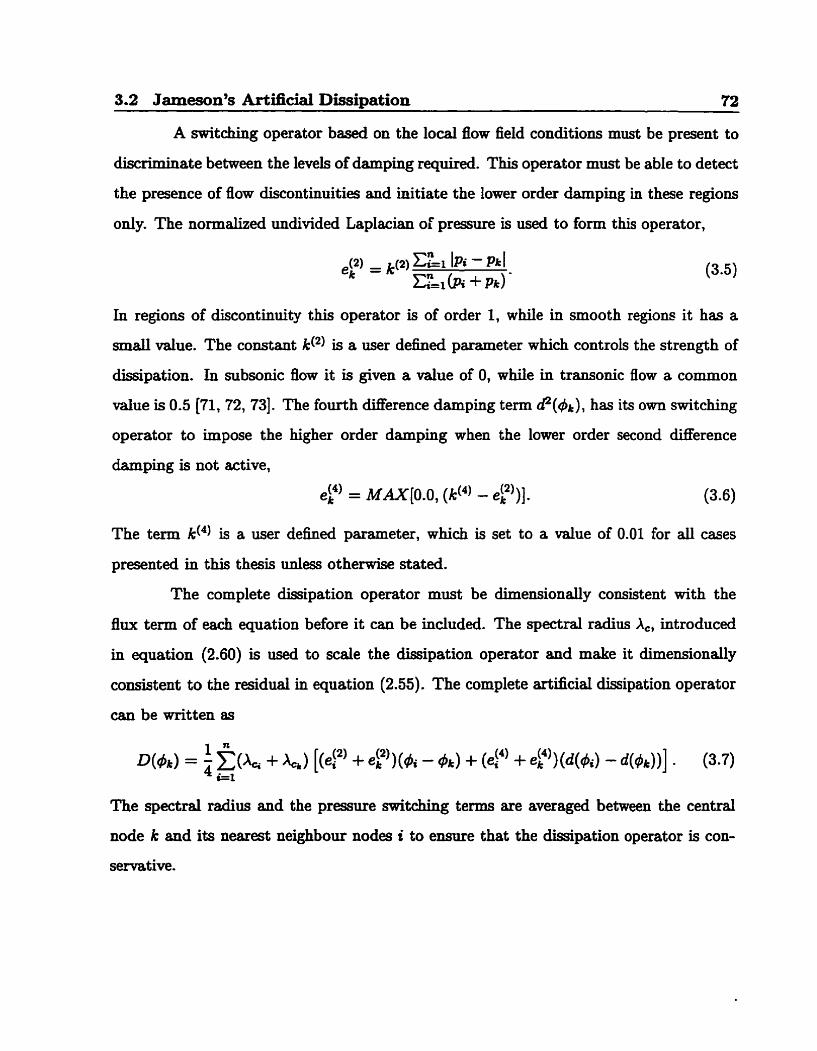
A switching operator based on the locd flow field conditions must be present to

discriminate between the levels of damping required. This operator must be able to detect

the presence of fiow discontinuities and initiate the lower order damping in these regions

ody. The normalized udivided Laplacian oiC pressure is used to form this operator,

In regions of discontinuity this operator is of order 1, while in smooth regions it has a

small value. The constant k(*) is a user defineci parameter which controls the strength of

dissipation. In subsonic flow it is given a value of O, while in transonic flow a common

d u e is 0.5 [71, 72, 731. The fourth Merence damping term dZ (~JJ, has its own switching

operator to impose the higher order damping when the lower order second Merence

damping is not active,

The term k(4) is a user defineci parameter, which is set to a value of 0.01 for all cases

presented in this thesis unless otherwise stated.

The complete dissipation operator must be dimemiondy consistent with the

flux term of each equation before it can be included. The spectral radius &, introduced

in equation (2.60) is used to scale the dissipation operator and make it dimensionally

consistent to the residual in equation (2.55). The complete artincial dissipation operator

can be written as

The spectral radius and the pressure switclhing tenns are averaged betweeo the central

node k and its nearest neighbour nodes i to ensure that the dissipation operator is con-

semative.

3.3 Stretched Artificial Dissipation 73

3.3 Stretched Artificial Dissipation

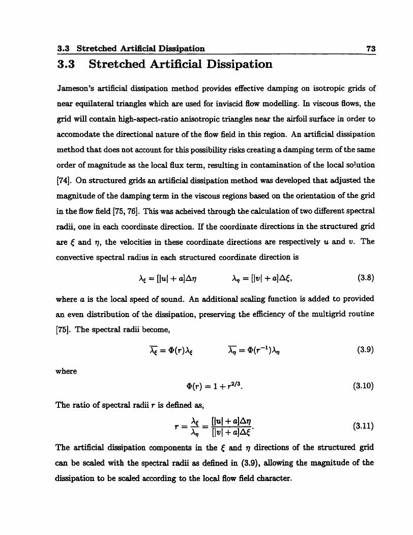
Jarneson's artScid dissipation method provides effective damping on isotropie gnds of

near equilateral triangles which are used for inviscid flow modeiling. In viscous flows, the

grid will contain high-aspect-ratio anisotropic triangles near the airfoil d a c e in order to

accomodate the directional nature of the flow field in this region. An artficial dissipation

method that does not account for this possibility risks creating a damping tenn of the same

order of magnitude as the local flux tem, resulting in contamination of the local so!ution

[74]. On structured grids an artificial dissipation method was developed that adjusted the

magnitude of the damping term in the viscous regions based on the orientation of the grid

in the flow field [75,76]. This was acheived through the calculation of two different spectral

radii, one in each coordinate direction. If the coordinate directions in the structured @d

are and r) , the velocities in these coordinate directions are respectively u and v. The

convective spectral radius in each stmctured coordinate direction is

where a is the local speed of sound. An additional scaIing function is added to providecl

an even distribution of the dissipation, preserving the efEciency of the multigrid routine

[75]. The spectrai radii become,

where

a(,) = 1 + rai3.

The ratio of spectral radii r is d&ed as,

The artificial dissipation components in the < and q directions of the ~ t ~ C t ~ e d grid

can be d e d with the spectral radii as defined in (3.9), dowing the magnitude of the

dissipation to be d e d according to the local flow field character.

3.3 Stretched Artificial Dissipation 74

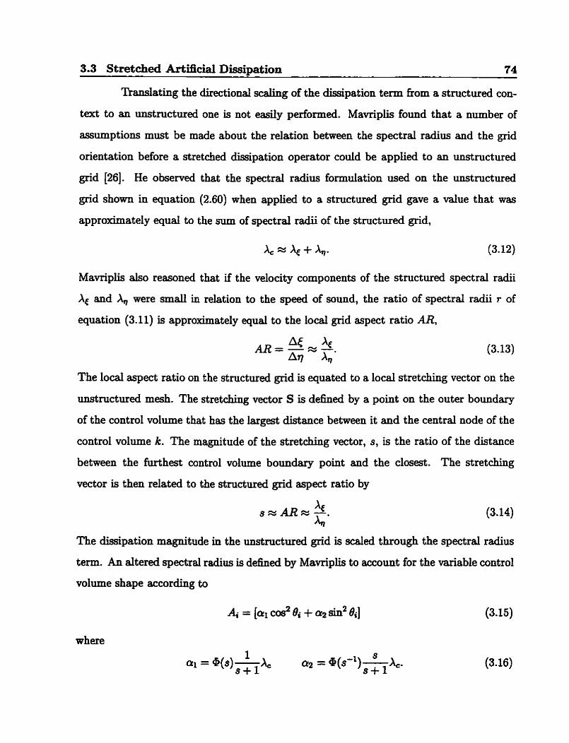
'I1ansIating the directional scaluig of the dissipation term fiom a çtmctured con-

text to an unstmctured one is not easily performed. Mavriplis found that a number of

sssumptions must be made about the relation between the spectral radius and the grid

orientation before a stretched dissipation operator could be applied to an unst ructured

grid [26]. He obsewed that the spectral radius formulation used on the unstructurecl

grid shown in equation (2.60) when applied to a structureci grid gave a value that was

approximately equal to the sum of spectral radii of the structured grid,

Mavriplis also reasoned that if the velocity components of the structurecl spectral radii

Ac and 4 were s m d in relation to the speed of sound, the ratio of spectral radii r of

equation (3.11) is approximately qua1 to the local grid aspect ratio AR,

The local aspect ratio on the strnctured grid is equated to a local stretching vector on the

unstructured mesh. The stretching vector S is defined by a point on the outer boundary

of the control volume that has the largest distance between it and the central node of the

control volume k. The magnitude of the stretching vector, s, is the ratio of the distance

between the furthest control volume boundary point and the closest. The stretching

vector is then related to the structureci grid aspect ratio by

The dissipation magnitude in the unstructured grid is scaled through the spectral radius

term. An dtered spectral radius is defined by Mavriplis to sccount for the variable control

volume shape according to

where

3.4 Higher Order Artaciai Dissipation 15

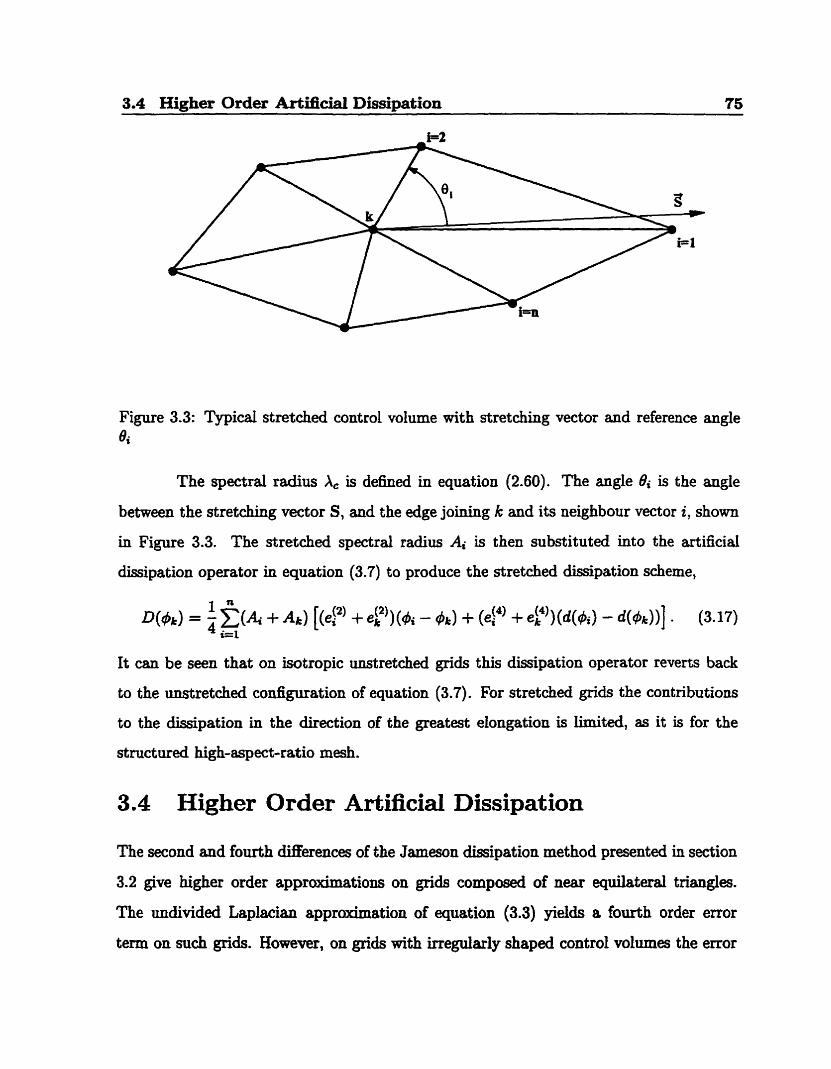
Figure 3.3: Typicd stretched control volume with stretching vector and reference angle 4

The spectral radius A, is defined in equation (2.60). The angle Bi is the angle

between the stretching vector S, and the edge joining k and its neighbour vector i, shown

in Figure 3.3. The stretched spectral radius 4 is then substituted into the artificial

dissipation operator in equation (3.7) to produce the stretched dissipation scheme,

It can be seen that on isotropie unstretched grids this dissipation operator reverts back

to the unstretched configuration of equation (3.7). For stretched grids the contributions

to the dissipation in the direction of the greatest eiongation is limited, as it is for the

structured high-aspect-ratio mesh.

3.4 Higher Order Artificial Dissipation

The second and fourth dineremes of the Jarneson dissipation method presented in section

3.2 give higher order approximations on grids c o m p d of near equilateral triangles.

The undivided Laplacian apprcnrimation of equation (3.3) yields a fourth order error

term on such grids. However, on gnds with irregularly shaped control volumes the e m r

3.4 Higher Order Artificial Dissipation 76

cancellation of the lower order terms in the Taylor series, which gives the higher order

approximation on the regular mesh, does not occur. The undivided Laplacian operator

will then approxhate not only the desirecl disapative terms, but also a number of first

order convective ones. The presence of these terms can create a significant contamination

of the local solution on irreguiar grids. Ideally, the dissipation operator should have a

negligible magnitude when the solution is smooth. In most cases the converged solution

wiII be a p p r h a t e l y linear over each control volume, and the dissipation should be s m d .

In the extreme case where the local solution is entirely h e a r , a dissipation method based

on a higher order Laplacian approximation will have a zero magnitude regardless of the

control volume shape. A dissipation method that approximates first order convective

tenns will have a non-zero magnitude in most such circumstances. The local solution

will be erroneously altered to compensate for the spurious flux created by lower order

dissipation methods which approximate these terms.

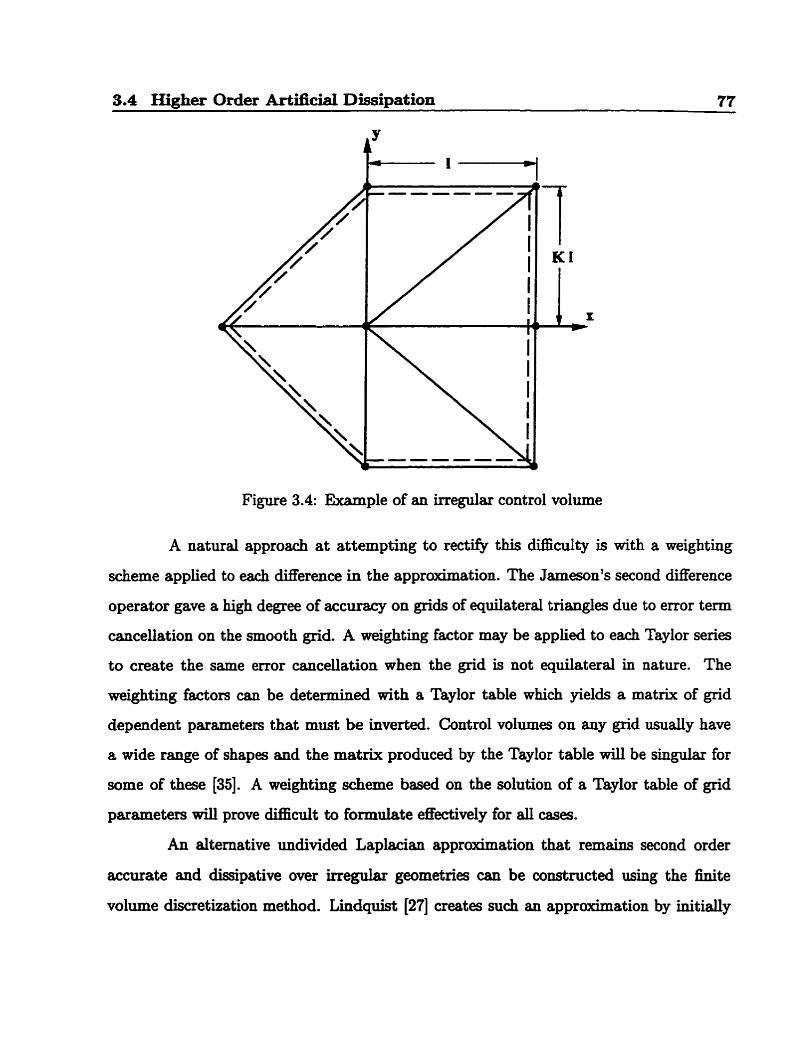
The potential for solution contamination by lower order dissipation has been in-

vestigated by Wilkinson [62] on a nurnber of irregular control volume shapes. An example

of which is shown in Figure 3.4. A two-dimemional Taylor series approximation can be

written for the solution at each neighbour node i in the same manner as was used for the

derivation of the difference expression of (3.3). Writing the resulting terms of the second

ciifference approximation yields the expression,

The fust term approximated by this difference expression on this control volume

is £imt order and convective in nature. A linear solution applied over such a control

volume can cause this dissipation operator to corrupt the local solution. As the gradient

on the linear solution inmeases, the magnitude of the dissipation operator will grow, even

through the local solution is linear. Near airfoi1 surfaces where gradients are relatively

high, irreguiar control volumes can reduce the 8ccuracy of the solution when a simple

clifference methad is used to a p p r h a t e diffusive terms.

3.4 Higher Order Artifidal Dissipation 77

Figure 3.4: Example of an irregular control volume

A natural approach at attempting to rectify th% difliculty is with a weighting

scheme applied to each clifference in the approximation. The Jarneson's second difference

operator gave a high degree of accwacy on grids of equilateral triangles due to error term

cancellation on the smooth grid. A weighting factor may be applied to each Taylor series

to create the same error cancellation when the grid is not equilateral in nature. The

weighting factors can be determined with a Taylor table which yields a matrix of grid

dependent parameters that must be inverted. Control volumes on any grid usually have

a wide range of shapes and the matrix produced by the Taylor table will be singular for

some of these [35]. A weighting scheme based on the solution of a Taylor table of grid

parameters will prove difficutt to formulate effectively for all cases.

An alternative undivided Laplacian apprdmation that rem- second order

accurate and dissipative over irreguiar geornetries c m be constructeci using the finite

volume discretization method. Lindquist [27] creates such an approximation by initially

3.5 Higher Order Stretched Dissipation

reducing the Laplacian using,

The higher order second dinerence operator can be con~tnicted by discretization of the

right hand side,

This difference operator is determined through an integration of the first derivative con-

vective terms about a control volume boundary, similar to the f i t e volume discretization

method. The operator is not divided by the control volume area, yielding an undivided

Laplacian approximation. The convective terms on each boundary edge are evduated

over the triangular c d of the control volume that contains the edge. The derivative for-

mulations of equations (2.53) and (2.54) are used on each triangle of the control volume

with integration conducted over each t n ~ g l e boundary. Derivatives are edua ted on each

control volume triangle as opposed to the control volume of each boundary node for two

reasom. First, integration about the three edges of each triangle is less computationdy

intensive than integration about the approximately six edges that form an average con-

trol volume boundary. Second, determinhg the second difference expression using only

information fiom the control volume maintains the local nature of the operator. This

differencing method creates an operator that is second order accurate and entirely dissi-

pative. This can clearly be seen by considering an irrepuiar control volume over which an

entirely linear solution is imposed. The convective terms will be constant over the control

volume and integration will yield a zero value of the diffaence operator, regardless of

the control volume shape. The fourth Merence free stream smoothing operator can be

constructed by using the higher order second Merence formulation with equation (3.4).

3.5 Higher Order S tretched Dissipation

The undivided LaplaQan approximation presented in the previous section was shown to

give second order sccuracy on irregularly shaped control volumes. This has the potential

3.5 Higher Order Stretched Dissipation 79

to provided smooth, highly accurate solutions on complex unstructured grids that contain

considerable irregularity. Adapted grids can be expected to be more irregular than an

unadapted mesh as a result of the adapted node placement. An effective higher order

artificial dissipation will be a complement to an adaptive solver. It has been shown that

the higher order dissipation method provided in the previous section was able to maintain

the second order spatial accwacy of an unstmctured central Werencing type scheme on

an irregular mesh with inviscid flow [27].

This artificial dissipation method can however encounter instabilities on viçcous

problems. The high-aspect-ratio control volumes near the surface of aVfoils can cause the

magnitude of the dissipation term to be exaggerated, even when the grid is smooth. This

can be demonstrated by considering an arbitrary control vohme over which is imposed an

entirely linear solution; #(x, y) = az + by + c. At the central node of this control volume

an error of magnitude is added (see Figure 3.5). Following the numbering scheme shown

in Figure 3.2, the first derivative terms at ceil A are cornputeci,

where AA is the area of triangle A. Simüar expressions are denved for each of the other

edges about the control volume. The higher order second Merence expression can be

created using equation (3.20). The contribution to the second ciifference from edge 1-2 is,

Summing all of the contributions fkom each edge leads to the final second difference

expression,


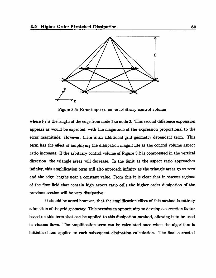
Figure 3.5: Error imposed on an arbitrary control volume

where 112 is the length of the edge fkom node 1 to node 2. This second difference expression

appears as would be expected, with the magnitude of the expression proportional to the

error magnitude. However, there is an additional grid geometry dependent term. This

term has the effect of amphfjhg the dissipation magnitude as the control volume aspect

ratio increases. If the arbitrary control volume of Figure 3.2 is compresseci in the vertical

direction, the triangle areas will decrease. In the Mt as the aspect ratio approaches

infini@, this amplification term will also approach infini@ as the triangle areas go to zero

and the edge lengths near a constant value. Rom this it is clear that in viscous regions

of the flow fidd that contain high aspect ratio ce& the higher order dissipation of the

previous section will be very dissipative.

It should be noted hocRever, that the amplification effect of this method is entirely

a function of the grid geometry. This permits an opportunity to develop a correction factor

based on this term that csn be applied to this dissipation method, allowing it to be used

in viscous flows. The ampUcation term can be calculated once when the algorithm is

initialized and applied to esch subsequent dissipation calculation. The final corrected

3.5 Higher Order Stretched Dissi~afion 81

higher order undivided Laplacian approximation can be written as,

The higher order nature of this artincial dissipation method with the amplification

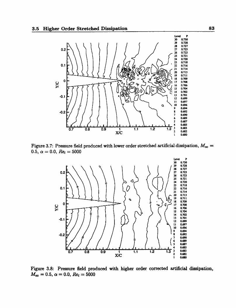
correction c m be demonstrated with the calculation of a flow field problern. The pressure

field is computed near the trailing edge of a NACA 0012 aidoil using both the stretched

iower order dissipation and the higher order method. The free stream Mach number is

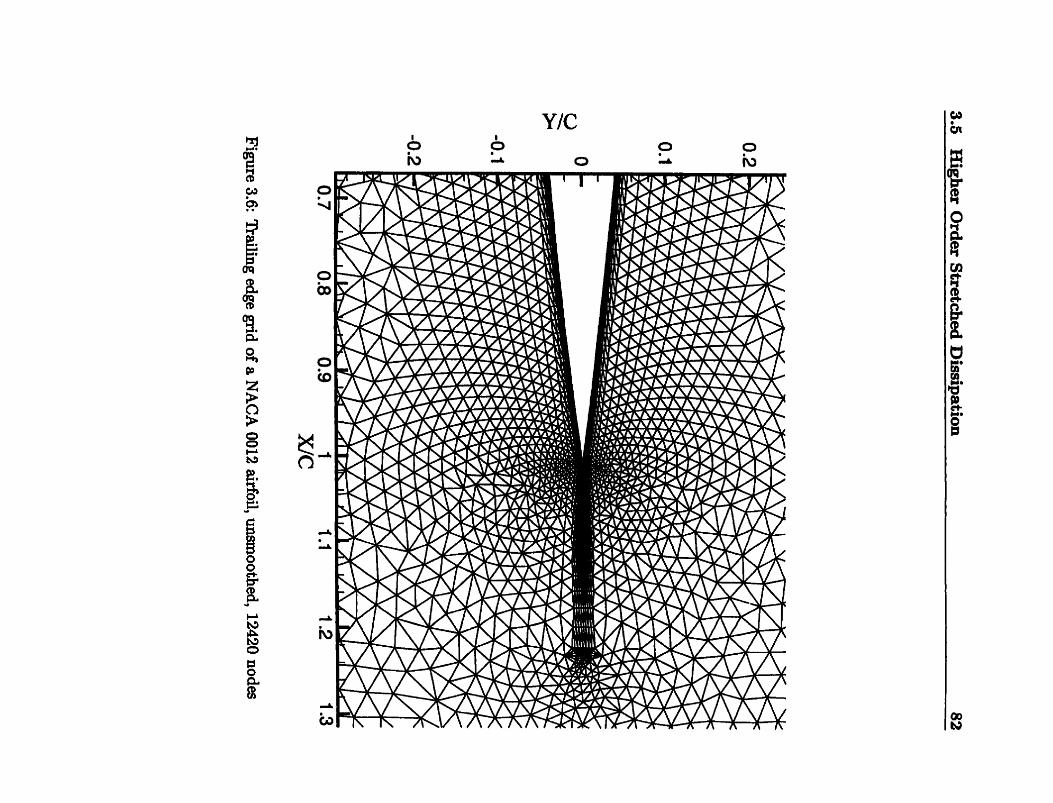
0.5 at 0.0 degrees angle of attack with a Reynolds number of 5000. Figure 3.6 shows the

tail region of the unsmoothed grid which contains numerous irregular control volumes.

The pressure field determineci using the stretched artificial dissipation method of section

3.3 is given in Figure 3.7. The corresponding pressure field computed with the higher

order corrected method is shown in Figure 3.8. The flow field about this airfoil is fkee of

shockwaves and should have a smoothly varying pressure field. The higher order corrected

dissipation produces a smoother pressure field than its lower order counterpart. This

suggests that the higher order method is less sensitive to the irregular control volumes

and high gradients present near the trading edge of this case.


Figure 3.7: Pressure field produced with lower order stretched artificiai dissipation, M, = 0.5, ai = 0.0, Rel = 5000

Figure 3.8: Pressure field produced with higher order correctecl artificial dissipation, M . = 0.5, O = 0.0, Rer = 5000

Chapter 4

Solution Adaptation

4.1 Motivation

The local truncation error in a numerical mode1 based on a central Merence f i t e volume

scherne is presented in Appendix B. The leading error terms are proportional to the second

and third derivatives of the total flux components in the x and y directions, and to the grid

conûguration expresseci through local edge length parameters. Reducing the local error for

a given problem has traditionally been accomplished through either a local Unprovernent

in the order of accuracy of the discretkation method itself or with some alteration of the

local grid characteristics. In this research, error reduction is achieved through refinement

of the grid using local node addition. Inserting an additionai node at the midpoint of each

edge in the grid will reduce each grid length parameter appearing in the truncation error

by half. In this manner the local t ~ n c a t i o n error can be reduced uniformly over the entire

grid in a 'global refinement' process. Although a global rehement is assureci of improving

the solution accuracy, renning each edge of an unstructured grid will inctease the number

of nodes by a factor of four, and substantidy increase the computational effort needed

for a solution. Repeated global refinements will only compound this increase in effort.

When it is considered that the laxgest truncation errors are predominantly located in or

nesr boundary layers, d e s , shock waves, and stagnation points, the wastefulness of a

global refinement becornes apparent. Additional nodes placed in free stream or smooth

regions of fiow have little influence on the global solution accuracy. If the edge refinement

4.2 Adaptation parameters 85

process is directed to occur in regions expected to contain a relativeiy high degree of

error only, the number of nodes needed for a global increase in accuracy will be less than

that of the global refhement. The process of detecting the error and locally refining and

restructuring the grid is the essence of the adaptive gridding process presented in this

t hesis .

Adaptive gridding in a h i t e volume soIver can be conducted using either a node-

additive (h-adaptive) method, or in a node-redistibutive ( r-adaptive) manner [24]. The

node-redistribution method does not insert additional nodes into the mesh but simply

rnoves the preemsting ones in an attempt at local error reduction. The improvement in

solution accuracy in one region may corne at the expense of another region as nodes are

removed fiom it. One common method of implementation of such schemes is with the

spring analogy formulation, where the edges that join a node to its nearest neighbours

are considered to act as springs. The spring constants are proportional to the local error

estimate on the edge, causing the edge iength to be shortened as an equilibriurn position

is found [53, 51, 781. The nodeadditive method introduces new nodes into the grid at

points specified by a local error indicator. New nodes are located at the midpoint of each

edge that is found to have a high levei error associated with it. Once all of the designated

edges have been rehed, the grid edges are reoriented to recover a smooth configuration

in a process referred to as retriangulation. The details of the adaptive gridding routine

used in this algorithm are presented in the following sections.

4.2 Adaptation parameters

The primary adaptation tool of this algorithm is a node-additive scheme. The adaptation

procers begins with the partidy convergeci solution on the finest grid. Convergence is

indicated by the summation over all control volumes in the computational domain of the

residuals of the mass conservation equation. Typically, when this total residual &op 1.5

orders of magnitude £kom its initial value, adaptation is initiated. Critical features of the


solution, such as boundary layers, wakes, and shock waves, will be well developed by this

point. Convergence hom the start dom to this level of residual is usuaily quite rapid

as the low fiequency errors are removed quickly by the multigrid routine. Any further

time marching beyond this IeveI will not contribute to the effectiveness of the adaptation

routine and will only consume computational resources. Fiirthermore, the final solution

will be obtained on the adapted grid, therefore, as Little effort as possible should be spent

on any intermediate grid.

The adaptation routine begins with the complete reproduction of the grid and

solution in the cornputer memory. The new adapted grid will be generated nom the

copied version. A completely new grid is created since the adapted grid wiil become the

new finest grid in the multigrid sequence. After the grid and solution are copied, the

adaptation proceeds with the selection of edges for rehernent. The edges selected are

determined by the dculation of an adaptation panuneter on each edge. The value of

the parameter gives an indication of the prionty assignecl to this edge in the adaptation

hierarchy. The adaptation parameter of each edge is then placed in descending numerical

order. A specific number of edga are selected by the user for adaptation. The multigrid

routine has providecl effective convergence acceleration when unadapted gnds have had an

appraimate four-fold increase in the number of nodes fkom coaRest to finest. In general,

this rate of increase in node density is maintained as new adapted @ds are generated.

Creating a factor of four increase in the number of nodes as a new adapted grid is created

would require that every edge in the parent grid be selected for adaptation. Since this will

defeat the purpose of adaptive gridding, adaptation is conducted in two passes. The user

WU specify the percentage of nodes to be selected in each pass as a &action of the total

number of edges in the parent grid. The adaptation passes are conducted consecutively

without using the solver between. Any particular triangle in the parent grid then has the

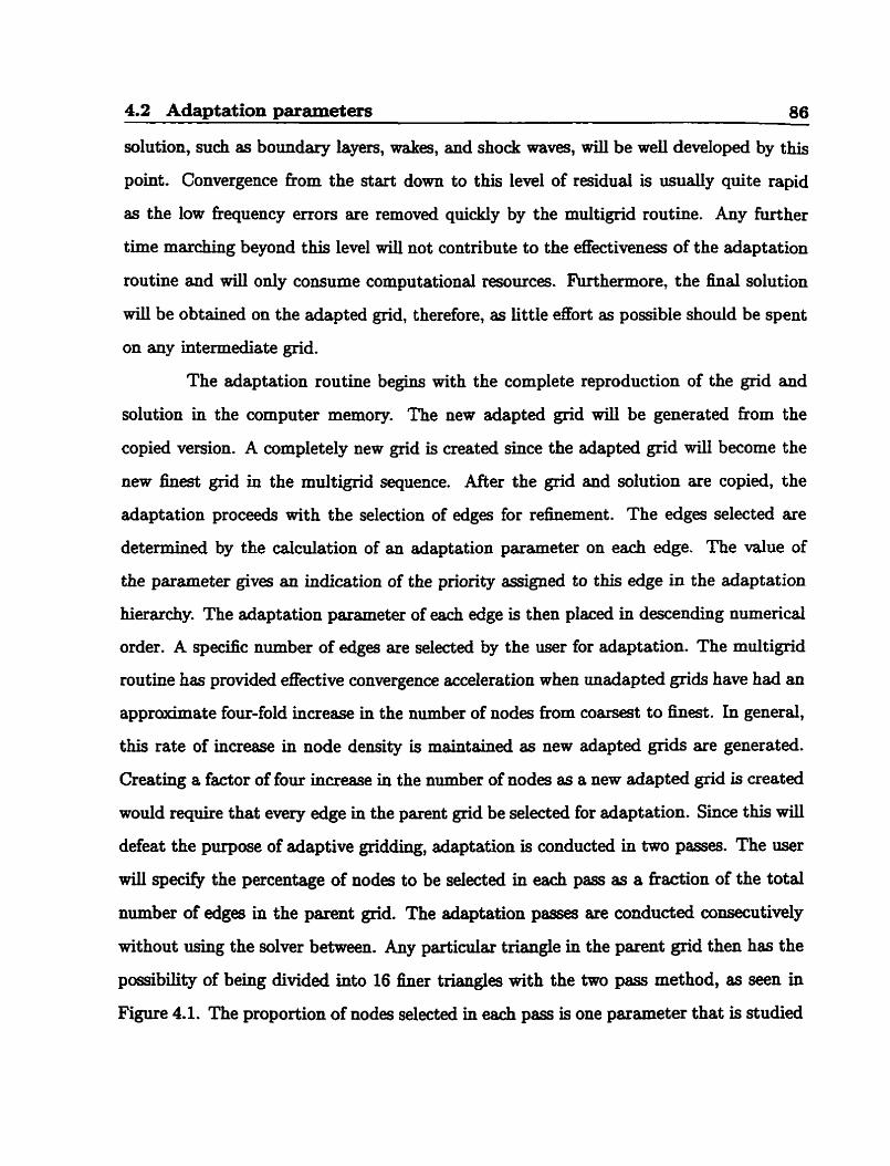
pmibility of being divided into 16 finer triangles with the two p a s method, as seen in

Figure 4.1. The proportion of nodes selected in each pass is one parameter that is studied


for its effect on solution iu:curacy in Chapter 5.

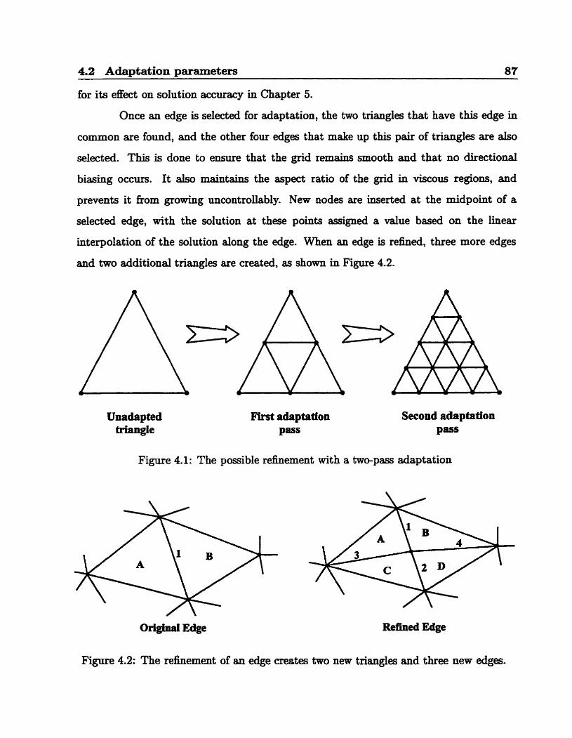
Once an edge is selected for adaptation, the two triangles that have this edge in

common are found, and the other four edges that make up this pair of triangles are also

selected. This is done to ensure that the grid remains smooth and that no directional

biasing occurs. It also maintains the aspect ratio of the grid in viscous regions, and

prevents it fkom growing uncontroIlably. New nodes are inserted at the midpoint of a

selected edge, with the soiution at these points assigned a value based on the h e a r

interpolation of the solution dong the edge. When an edge is refined, three more edges

and two additional triangles are created, as shown in Figure 4.2.

Unadapted triangle

First adaptation P*S

Second adaptation P=s

Figure 4.1: The possible rehernent with a two-pass adaptation

Figure 4.2: The refineement of an edge creetes two new triangles and three new edges.


The adaptation parameter can be calculated using any one of a number of philoso-

phies. The parameter is intended as an estimate of the error in the solution resulting hom

the local grid contiguration. The direct approach to the creation of an adaptation pa-

rameter wodd be a calculation of the local tnincation error of the spatial discretization.

Appendùr B gives an estimate of such an error term. The truncation error contains second

and third derivatives of the flux temm scaled with terms dependent on the local grid con-

figuration. The tmcation error is not a practical choice for the adaptation parameter in

this algorithm for several reasons. First, calculation of both the second and third deriva-

tive flux terms wilI be necessary since the grid dependent scaling terms on the second

derivatives will vanish in the presence of grids composed of near quilaterd triangles. On

inviscid portions of the flow field the grid will be c o m p d entirely of near equilateral

triangles. Secondly, a significant amount of computational effort will be needed to deter-

mine second and third derivatives of the flux components at each node. A least squares

polynomial approximation using the solution obtained from the surrounding grid cm be

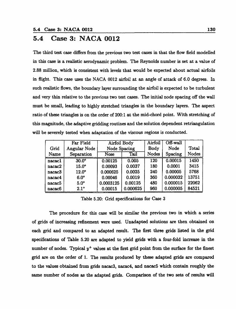
created that will permit the evaluation of second and third order derivatives However,

such rnethods may s d e r fiom inaccuracies, especially near flow discontinuities like shoek

mves. The third difEculty encolmtered when using the truncation error as an adaptation

parameter results fkom increased sensitivity. Since the adaptation routine uses a partially

converged solution as a staxting point, some high frequency error d still rernain. For

an error of hed magnitude the second and third derivatives of the solution will give in-

creasingly larger values. This can be demonstrated by considering a one-dimensional gid

with sn erroneous solution imposed on it of the fom,

where A is the amplitude and 1 the wave length. Second and third derivatives of this

solution will yield the following values,


As the wavelength shrinks, the amplitude of the second and third derivatives of the

solution will grow considerably. An adaptation parameter using such terms will have

an exaggerated magnitude compared to the amplitude of the error. In this instance,

adaptation will be driven by the high frequency error and less by the flow field features.

Additional nodes may well be placed in regions that in fact are found to be well resolved

without them, thereby wasting computational effort. Fùrthermore, a greater degree of

convergence prior to adaptation is not always successful at removing difEculties of this

nature. The caldation of the second and third derivative components of the leading

truncation error terms assumes that the continuous solution of the flow field is known.

If this known continuous solution is apprcarllnated with the numerical solution, as would

be the case, any discontinuities in the numerical result may lead to inflated estimates of

truncation error. This algorit hm produces piecewise linear continuie between triangles,

but not continuity of slope. On a coarse grid a M y converged solution may have slight

discontinuities in slope between triangles sufficient to cause erroneous estimates of the

second and third derivative tnuication error components.

Another possible adaptation parameter assumes that bcal error is associated with

the rate of change of the flow variables, and uses the field gradients dong each edge of

the domain. These are easily computed dong each edge by differencing the field variable

(q) between the two nodes that d e h e an edge (i j) and nomaliPng by the edge length 2

Unlike second and third derivative approximations which can contain some error, terms

computed in this rnanner are an exact representation of the derivative of the field variables

dong an edge since the numerid solution given on each edge is linear. However, an adap

tation parameter based on first derivatives wiU suffer fiom the same error exaggeration as

the tnuication term parameter, although to a lesser extent. One critical dificul@ expe-

rienced when using flow gradients as adaptation parameters was investigated by Warren

et al. [43]. They found that repeated adaptations would place new nodes at the same


location in the %ow field, regardless of the local level of refinement. Once an edge was

selected for adaptation, the new node placed at its midpoint would be given field variables

based on the linear average of the values at the edge endpoints. The two new edges will

then have exactly the same field gradients as the original edge. Consecutive adaptations

using gradients to dwct refinement wiU then be confined to the same features in the

flow field. Idedy, an adaptation parameter should be rdective of the local level of error

reduction with repeated refinement. As additional nodes are placed in a region, the local

truncation error wi l l be reduced. An adaptation parameter that reduces its value to reflect

the improved local resolution will permit repeated adaptations to redirect refinement to

regions that then become the most under resolved.

The difEculty ansociated with the edge gradient as an adaptation parameter stems

from the fact it is divided by the edge length. Under repeated adaptations the edge length

will be reduced by the same factor as the fieId variable clifference, thereby preserving the

value of the gradient. An alternative formulation is to omit the edge length and adapt

on an undivideci dinerence. An adaptation parameter based on undivided differences will

require very little computational expense. It will also maintain a fixeci magnitude in

the presence of an oscülating error of constant amplitude, regardless of the wavelength.

F'urthermore, the undivided difference will drop in magnitude after repeated adaptations

on a given solution, similar to the expected behaviour of the actuai tnincation error after

such rehernents.

An adaptation parameter based on undivided Merences can use any of the a d -

able flow field variables. Numerical experiments on inviscid aerodynamic problems have

been conducted by Dannenhoffer [42] to determine the the most effective adaptation vari-

able. It was found that undivided differences of density were able to provide smooth

adapted regions and the m a t rapid convergence for a giwn level of arxuracy. In addi-

tion, it was also found that adaptation on second differences, similar to the Laplscian

approximation in artificial dissipation, created irregularly shaped adapted regions which

4.3 M o i l Boundary Adaptation 91

adversely effected the convergence rate. In the present algorith, a number of variables,

including densi@, pressure, Mach number, and vorticity, will be studied as adaptation pa-

rameters for their influence on solution accuracy for a given level of computational effort.

The undividecl clifference used as an adaptation panuneter (O) in this study, computed

between the two nodes ( i j ) that define an edge, will have the form

In this instance the parameter is calculateci as the combined dinerences of density ( p )

and Mach number (M) nomalized by the extreme Merence value over the grid. The

merences are normalized to d o w combinations of severd variables in the formation of

the adaptation parameter.

Airfoil Boundary Adaptation

Far fiom an airfoil surfice, a new node added through adaptation is simply placed at

the midpoint of an edge. On airfoil surfaces new nodes must proceed through a more

complex procedure. The edges that form the airfoil swface are an approximation to the

tme aidoil shape. The sctud shape of the aidoil is represented by a series of spline c w e s

that span the distance between the nodes that form the airfoil body 1791. If a new node is

added to the midpoint of an edge that forms the airfoi1 body, the original approximation

is preserved and not refined. Zn order to improve the aVfoil shape appromation, the

new nodes added to the Moi1 edges must be moved into the midspan locations suggested

by the spline curves. However, this may create difEculties on high-Reynolds-number

flows where the normal OW spacing of nodes is very s m d . The movement of the new

boundary node into the interior of the domain may cross pre-e)Listing edges. This problem

is graphically presented in Figure 4.3, where a section of the grid at an airfoil boundary is

shown. The spline representation of the Moi1 is shown as a broken line. The edges that

approurimate the airfoil surface are the heavy lines at the base of the grid. The location of

a new boundary point specined by the spline curve is indicated. Clearly, if a new node is


plsced at the midpoint of the boundary edge show, and moved to the location indicated

by the spline curve, a number of edges wil l be crossed over and the grid will be defective.

To overcome this difliculty, Mavriplis [50] developed a method of displacing ail

of the edges above these problematic boundary nodes. A line is & a m from the new

midpoint node in Figure 4.4, normal to the original edge into the interior of the corn-

putational domain. The edges that are crossed and the points of intersection on these

edges are recorded. The distance between the new midpoint node and its ha1 location

specified by the spline curve is caUed the reference length. The distance between the

new midpoint node and the h t intersection point of a crossed edge is computeâ. If this

distance is greater than twice the reference length, then the routine is terminated and the

new point is simply inserted at the boundary edge midpoint and moved into its proper

location. However, if this distance is l e s than twice the reference length then there is a

possibility of creating crossed edges or triangles with areas near zero. In this instance,

the distance between the next pair of intersection points dong the normal h e is deter-

mined. Consecutive pairs of intersecting points are checked until their spacing is twice

the refewice distance. At th.& point the process is stopped snd ail edges crossed have

new nodes inserted at their intersection points. This column of nodes is moved with the

new boundary node as it is placed in its proper location. The new grid configuration will

then be the defect fiee mesh shown in Figure 4.5.

Figure 4.3: The portion of the grid forming the d o i l boundary. A new node is to be inserted at the body edge midpoint.


- New boundary point 0 - Normal Une intersedon point

- - Airfofl body approximation - - - Splhe curve

Figure 4.4: A line normal to the boundary edge is drawn through the interior grid, marking points of intersection.

Figure 4.5: The new boundary node is moved to the location specsed by the sphe routine, the column of nodes above it moves in conjunction.

4.4 Solution Adaptive Retriangulation 95

4.4 Solution Adaptive Retriangulation

Once additional nodes have been introduced into the grid in an adaptation procedure,

the srnoothness of the original grid is usually lost. The @cl edge orientation that resulted

in control volumes of approximately six near equilaterd triangles will most certainly be

dismpted. It was shom in Appendix B that control volumes composed of six near-

equilateral triangles attain a second order spatial accuracy. In order to preseme this

spatial accwacy on inviscid portions of the flow field, the edges of the adapted grid must

be re-oriented in a retriangulation process to recover an equilateral configuration. The

Minmax triangulation procedure described in section 2.7 was used to generate grids of

near eqdaterd triangles. This routine is used again in the adaptive gridding procedure

to recover the eqda te rd configuration.

The Minmax retriangulation is imposed tbough a global edge swapping routine.

Every non-boundary edge is assessed to determine if it meets the Minmax criterion. This

is done by considering the pair of triangles that have a given edge in C O ~ O ~ , as shown

in Figure 4.6. The common edge is in one of two possible configurations, the second

configuration in the figure is represented by the broken %e. The largest of the six intenor

angles of both configurations is determined, and the orientation that minimizes this angle

conforms to the Minmax criterion. Every interior edge in the computational domain is

assessecl in this manner until no more edges need to be reconfigured.

On inviscid regions of the flow field the Minmax retriangdation will easily recover

a near-equilangular grid. In regions of the grid expected to be dominated by viscous ef-

fects, the grïd is characterized by stretched high-aspect-ratio triangles. The sdaptive

gridding routine can disrupt the structured node placement of this region in such a man-

ner that the Minmax retriangulation procedure creates near-equilateral triangles as it

does in the inviscid regions. For example, Figure 4.7 shows a high-aspect-ratio portion of

a grid near an airfoil. A new node is added which introduces a degree of irrepuiarity into

the local node placement. The Minmax retriangulation, shown in Figure 4.8, generates

4.4 Solution Adaptive RetrianRulation 96

Figure 4.6: The angles considered in the Minmax edge-swapping triangulation. The broken line indicates the other possible edge configuration.

near-equilateral triangles in regions where the grid is expected to be highly stretched.

The presence of such triangles within boundary layer regions will introduce severe tm-

cation error. To prevent the possibili3 of such undesirable retriangulations, the grid is

stretched in the direction of the local Mach number gradient before the retrianguiation is

implemented. Once the Minmax criterion is imposed, the grid nodes are returned to their

previous location. Initially, the gradient of the Mach number is found on the four nodes

of the pair of tnmgles that shsse a common edge. These values are averaged to give one

pair of derivatives valid on the edge itself (M,,M,). The stretching parameter Si is used

to temporarily place the four nodes in their stretched locations (X,',Y;.'),

The lengths Axi and Ayi are the distaces in the z,y coordinate directions fiom the

midpoint of the edge to each of the four surrounding nodes. The location X,O,y,O is the

original location of the node. The term 1 is the length of the edge, and ( is a small positive

value used to avoid singularities. The factor C is used to s a l e the stretching effect and

is set at a value of 2.0. The resulting grid &ter the stretched Minmax retriangdation is

shown in Figure 4.9. The grid retaim the stretched nature desired in the viscous regions.

4.4 Solution Adaptive Retriangulation 97 - - - - --

The modified retriangulation method is now solution adaptive in nature since it now

reconfigures the grid based on the local flow field conditions.

The eff'tiveness of the stretched Minmm retrimgulation in maintaining a smooth

grid configuration can be demonstrated through the folIowing example. An adapted grid

is generated fkom the solution about an airfoil at a Reynolds number of 500, and 0.0

degrees angle of attack. The adapted grid without retriangulation displays a significant

level of irreguiarity as seen in Figure 4.11. The retriangulated version, seen in Figure 4.10,

clearly demonstrates the improvement afforded by such a process. Near the airfoil body,

Figure 4.12 shows the adapted grid dter retriangulation using the undterd Minmax

routine, while Figure 4.13 shows the r d t s of the stretched retriangulation. The regular

Minmax routine fkequently creates the near equilateral triangles that can be detrimental

to accurate boundary layer resolution. The stretched retriangulation is completely free of

such triangles.

Cg - New Node

Figure 4.7: A new node is introduced into a high-aspect-ratio region of the grid near an airfoîl d i t c e .

4.4 Solution Adaptive Retriangulation 98

t@ - New Node Figure 4.8: The Minmax retriangulation can generate near equilateral triangles in high- aspect-ratio regions of adapted grids.

- New Node

Figure 4.9: The stretched Minmax retrimgdation ami& creating near equilateral trian- g1es in high-aspect-ratio regions of adapted grids.

4.4 Solution Adaptive Retriandtion

Figure 4.10: Adapted grid, with retriangulation

Figure 4.11: Adapted grid, no retrianpuiation

4.4 Solution Adaptive Retrianguiation 100

Figure 4.12: Adapted grid, stretched Minmax retriangulation

k 1 I I I 1 1 i I i l i 1

0.1 0.2 W C

Figure 4.13: Adapted grid, reguiar Minmax retriangulation showing inappropriate triangles in the high-aspect-ratio regions

Chapter 5

5.1 Test Cases

Previous chapters have presented the details of the adaptive finite-volume solution algo-

rithm. This chapter presents the results of six test cases based on aerodynamic problems

which will permit an assessrnent of the performance of the algorithm. TWO test cases will

be used to optimize the solution adaptive gridding routine such that the lift and drag

coefkients predicted by the algorithm will be as close as possible to the grid independent

result for a given number of grid nodes. The test cases were selected to provide a wide

range of flow field conditions over whkh the algorithm would be expected to perform.

Two laminar cases are included that contain both attached and separated boundary lay-

ers in addition to well developed wake regions. Four turbulent cases are presented which

provide a range of physidy reaiistic fight conditions. The foilowing table summarizes

the details of each test case.

Case 1 Case 2 Case 3 Case 4 Case 5 Case 6

Test Case

NACA 0012 NACA 0012 NACA 0012 NACA 0012 RAE 2822

AGARD AR 303 A2

M o i 1 Free Stream Mach Number

Table 5.1: Test Case Summary

101

Angle of Attack

10-0" 0.0" 6.0" 0.0" 2-70" 4.0"

Reyno1ds Number

500 5000

2.88x106 9.Ox1O6 6.50 x 106 3.52x106

Reference

[84 PSI [81]

[82,83] [84]

185,861

5.1 Test Cases 102

The multigrid convergence acceleration method requires a series of grids with

increasing rehement to perform properly. Grid refinement is imposed through successive

reductions in the off-wali spacing and node spacing on the aidoil body, in addition to

increases in the number of nodes that form the body. A grid series provides an ideal

opportunity to calibrate and assess the pedormance of the adaptive gridding routines. In

cases 1 and 3, the undivideci clifference of various flow variables and their combinations

are tested as adaptation parameters, dong with several variations on the number of

nodes adapted in each p a s . Solutions are obtahed on a series of grids generated through

adaptation and compared to results obtained on a co~~esponding series of unadapted grids

with an equident number of nodes. Given that the adaptive gridding scheme incurs only

an additional 3% to 5% in total computation t h e , grids with equivalent numbers of nodes

will incur approximately the same computational expense to achieve a solution. Therefore,

the mod effective adaptation configuration is the one which attains the smallest error in

lift and drag prediction for a given number of nodes. Fhrther evidence of the solution

improvement provided by the higher order artificial dissipation presented in section 3.4 is

examined in case 2. In each of the test cases the higher order artificial dissipation is used

d e s s otherwise stated. High speed flow is considemi in case 4 where a weli developed

sbock wave pattern emerges behind a NACA 0012 airfoil, presenting a good test for the

adaptive gridding routine. A cornparison is made in case 5 between the predicted surface

pressure and experimentally determineci values on a co~ll~llonly used test case using the

RAE 2822 airfoil. The final test case examines the results on a complex multi-dement

aidoil in a hi& lift configuration. T h e 1st four cases contain high-Reynollds-number flows

which require highly stretched grids in the viscous regions, providing challenging problems

for not only the Navier-Stokes solution routine but for the adaptation procedures as wd.

5.2 Casel: NACA 0012 103

5.2 Casel: NACA 0012

The first case is taken from the GAMM Workshop on Numerical Simulation on Compress-

ible Navier-Stokes flows [80]. It uses a NACA 0012 airfoi1 in a free stream flow of Mach

number 0.8 at an angle of attack of 10 degrees with a chord-based Reynolds number of

500. This case was selected since it exhibits an extensive solution field with a number of

flow features that are commonly encountered in viscous aerodynamic problems. The lower

surface of the airfoi1 experiences an attachecl boundary layer all dong its length, while

the upper airfoil surface encounters boundary layer separation very near the leading edge.

With a low Reynolds number of 500, viscous effects will dominate the flow field giving rise

to thick boundary layers and a well developed wake region extending far downstrearn of

the airfoil. Flow field variables such as the local Mach number, the density, the pressure

and vorticity will show large vaxiations extendhg far fkom the airfoil d a c e , providing an

ideal environment for testing and calibration of nurnerous possible adaptation parameten.

Tsble 5.2: Grid specifications for Case 1

The analpis begins with a series of five grids, starting with a corne me& of 752

nodes and ending with a fine g15d of 78,459 nodes. The outer far field boundary of each

Totd Nodes

752

@d is 60 chords fiom the airfoil d m with an 'O' shape identical to that shown in

Figure 2.16. The specifications for each grid are shown in Table 5.2 above. The far field

angular node separation is the distance between each outer b o u n d q node in degrees of

arc. This parameter is used to control the node density in the outlying regions of the

computational domain. The airfoil body node spacing is the initial body node separation

Off-wall Node

Spaci~g 0.01

Airfoi1 Body Nodes

60

Grid Name nacaal

Far Field Angular Node

Separation 20.0"

Airfoil Body Node Spacing Nose 0.004

Tai1 '

0.02

5.2 Casel: NACA 0012 104

mea~u~ed dong the camber line of the airfoil starting at both the leading and trailing

edges. Rekement is conducted by dividing in haIf each of the airfoil grid specifications

and doubling the number of nodes on the airfoil, yielding a global refinement.

As the node spacing is reduced through global refinement, the numerical error

in the solution is also diminished. After numerous consecutive refinements, the predicted

lift and drag of a particular problern will approach specific values. At this point the grid

independent values of Li2 and drag are obtained since any further rehements will yield

only insignificant changes. These values are of importance in determinhg the effectiveness

of an adaptive gridding method since they represent a solution with very Iow global

numerical error. An effective adaptive gridding strateg, will refine the regions of highest

local error initiaDy, rapidly reducing the global error. The lift and drag predicted by

adaptation can be compared to the grid independent values to meanire the progress

towards a low error state. The ultimate success of an adaptive gridding method is revealed

when, in cornparison to the unadapted global refinement, the adaptive method achieves

the low error state with far fewer nodes.

Grîd 1 Total 1 Lift Name 1 Nodes 1 Coefficient

0.5965 0.5208

Total Drag Pressure Drag fiction Drag Coefficient Coefficient Coefficient

O. 2840 0.1 709 0.1131 0.2695 0.1589 0.1 106 0.2629 0.1537 0.1092 0.2617 O. 1527 0.1090

Table 5.3: Unadapted liR and drag results for Case 1

Table 5.3 provides the predicted lift coefficient (C,), total drag coefficient (Cd),

fnction drag coeflicient (Cg), and pressure drag coefncient (C,) for the unadapted grids.

Comparing the d u e s of the two finest grids indicates that signifiant changes axe still

occurring with dnement, and therefore the grid independent solution has not yet been

reached. An dtemative to h d h g the solution on grids with extremely large numbers

of nodes is to extrapolate the grid independent solution from the known data. Since

5.2 Casel: NACA 0012 105

the corne grid resuits are expected to contain a high level of emr , only the data fiom

the hest three grids are used. After performing a linear regression on the data, the

grid independent solutions are obtained when the number of grid nodes is brought to

infinity. Figures (5.2-5.5) graphically show the data for the finest three grids and the

linear approximation to the results. The grid independent solution was found to be,

The optimal adaptation parameter is one that can direct grid refinement to re-

gions that contain si&cant error. Flow features that are expected to be regions of

numericd error such as shock waves and boundary layers require a high degree of res-

olution. However, Warren et al. [43] found that regions adjacent to such features also

contain significant error and must also be adequately resolved to obtain an accurate s*

lution. Therefore, the search for the most effective adaptation parameter focusses on

variables that offer the a b i l i ~ to detect critical features but also d o w adaptation of re-

giom near those fatures. The variables considered for the adaptation parameter are: the

flow field Mach number, densi@, pressure, and vorticity. These variables wil l be denoted

by 'M', 'd', 'p', and 'v' respectively in subsequent data tables. The solution field for each

of these variables obtained on grid nacaa2 is presented in Figures 5.6, 5.8, 5.10, 5.12. The

correspondhg series of adapted grids, generated using each of these variables as adapta-

tion parameters, is presented in Figures 5.7, 5.9, 5.11, 5.13. The adaptation is conducted

in two passes as outlined in section 4.2, with 55% of the nodes added in the first pass and

45% in the second. The unadapted grid nacaa2 is provided in Figure 5.1 as a reference.

The Mach number field shown in Figure 5.6 dehes the location of the boundary layer

and wake regions, but has a small variation in the regions surrounding these features. The

resulting adapted grid, shown in Figure 5.7, concentrates nodes primarily on the viscous

f a t u m at the expense of the surroundhg grid. The densi@ field shown in Figure 5.8 also

follows the viscous fatmes, but without the high level of variation as the Mach nurnber.

However, the density contains signinmt gradients in regions adjacent to these features

5.2 Casel: NACA 0012 106

where the Mach number does not. The adapted grid based on density in Figure 5.9 shows

that this feature leads the adaptation routine to refhe the grid over a more general area

at the expense of the viscous regions. This raises the possibility that a combination of

variables will provide the most effective adaptation parameter. The pressure field shom

in Figure 5.10, gives no indication of the viscous flow features, but contains strong vari-

ations near the Ieading edge of the airfoil, similar to the density. The correspondhg

adapted grid shows none of the viscous regions of the previous variables, but does give a

general refinement over the entire region surromding the airfoil. The absolute value of the

vorticiw, shown in Figure 5.12, contains strong gradients in the attached regions of the

boundary layer but nowhere else. Its adaptation places nodes in the attached boundary

layers exclusive1 y.

Assessrnent of the various possible adaptation parameters is conducted with a

series of adapted solutions. The first three coarsest grids in Table 5.2 are adapted to create

grids with the sarne number of nodes as the next finest grid. For instance, grid nacaal

WU be adapted to create a grid with the sarne number of nodes as nacaa2. In this manner

a direct cornparison c m be made between the results of the unadapted grids and their

adapted counterparts. The four variables under consideration are used to adapt each grid,

dong with combineci Mach number/pressure and Mach number/density formulations.

Three different node allocation schemes for each adaptation pass are considered as weU.

The k t allocation places 70% of the refinement nodes in the first pass and 30% in the

second. The next allocation uses 55% in the first and 45% in the second, while the last

method uses three passes each docated 33% of the refinement nodes. Tables 5.5, 5.7,

and 5.9 provide the Lift and drag coefücients for each of the adapted grids. Tables 5.6,

5.8, and 5.10 give the percentage error of each of these results in cornparison to the grid

independent dues. The percentage error of the unadapted results are listed in table 5.4.

Rom the results it is ckar that certain variable and allocation combinations

perform better that others. Comparing the unadapted error for the grid nacaa2 with the

5.2 Casel: NACA 0012 107

adapted error for pressure and vorticity adaptation, it is clear that these variables perform

poorly in general. The error for each lift and drag performance characteristic using these

two variables is comparable to the error level for the unadapted results at each grid size.

The inability of these variables to detect and adequately resolve all the regions that contain

a high level of error, compromises their capabiiity as adaptation parameters. Adaptation

parameters based on Mach number and density appear to fair better. At every adapted

grid level and for each node docation method the Mach number and density adaptation

had a lower error than the unadapted results for each performance characteristic. In fact

the error produced by these two adaptation variables is very similar, even though they

emphasize slightly different regions of the grid. For Instance, at the 2800 node level with

55%/45% allocation the lift error is 12.45% for the Mach number and 13.73% for the

density. The total drag error is similar with 5.07% for the Mach nurnber and 5.22% for

the density. Considering that the error for the unadapted grid is 17.4346 for lift and 9.06%

for total drag, these two variables have achieved a significant reduction in global error over

the unadapted grid. At the 10500 node level the results are similar, with lift and total

drag error at 4.74% and 2.42% respectively for Mach number and 4.76% and 2.15% fgr the

density. Since the Mach number and density r e h e somewhat different regions of the @d

and stiU obtain the ssme error reduction, it must be concluded that the regions that these

two variables refine are equally important to global error reduction. The effects of a linear

combination of these adaptation parameters was investigated. The results show that a

combined Mach number and density adaptation parameter with 5596145% allocation gives

the iowest error of any configuration. At the 2800 node level, the improvement in Mt error

over the unadapted results is appraximately 30%, while for total drag it is 44% with the

combined adaptation parameter. At the 10500 level, the rermlts are similar with a 30%

improvement in lift error and 34% for total drag.

Of the three node docation schemes for each adaptive pas, the methods that

use a 55%/45% distribution generally tend to produce less error. Comparing the error

5.2 Casel: NACA 0012 108 - .- - . -- -- . . - -- - . - . -. . -

for the Mach number or density adaptive parameters, the error in lift and drag is lower

for 55%/45% than 70%/30% at both 2850 nodes and 10500. This trend is l e s apparent

for the combined Mach number/density or Mach number/pres~ure adaptive parameten.

In the Mach number/density case the 5596145% docation remain superior. However, for

the Mach number/pressure case 70%/30% is best at 10500 nodes. The allocation method

with the poorest overd performance is the three p a s method. The lift and drag error

using this allocation is generdy larger than the other methods. For instance, the 1%

and total drag error at 2850 nodes for Mach number 55%/45% adaptation is 12.45% and

5 .O?% respectively. Using the three pass 33%/33%/33% method yields the values 15.06%

and 6.61% for lift and total drag error.

For the largest grid size, the adaptation results using either Mach number, density,

or both produce errors that are almost entirely below 0.5% of the grid independent value.

The fact that the results on this grid size are nearly identical to the grid independent

values inclkates that adaptation methods ushg these variables are capable of obtaining

the grid independent values of lift and drag with far fewer nodes than the unadaptecl global

refmement. Clearly, adaptation directed by edge clifferences is successful at detecting the

local error in a solution and reducing such error to produce a reduction in global error.

Further experirnents were conducted with multiple adaptation using combined

Mach nurnber/density and Mach nurnber/pressure parameters with both the 70%/30%

and 55%/45% node allocations. The coarsest grid, nacaal with 752 nodes was adapted

once to produce a grid of apprcarimately 2850 nodes and then again to yield a @d of

nearly 10700 nodes. Tables 5.11 and 5.12 give the Iift and drag results dong with the

e m r for the multiple adaptations. The results indiate that even further error reduction

is possible with multip1e adaptation. The best multiple adaptation liR and total drag

error is 3.27% and 1.46% respectively using the Mach number/densi@ 70%/30%. The

best results using one adaptation for an eqUiwent grid size yielàs values of 4.42% and

2.30%. The unadaptecl 1 3 and total drag error for this grid size is 6.27% and 3.49%.

5.2 Casel: NACA 0012 109

The double adaptation method therefore provides an approlcimate error reduction on the

order of 50% for both liR and drag over the unadapted grids. It shouid be noted that

the dinerence in error between the double adaptation Mach number/density 55%/45%

method and the 70%/30% version was süght.

The trends expresseci in this study of various adaptive methods are portrayed

graphically in Figures 5.145.17. The results of the unadapted grids are shown with

those of the two most effective adaptation methods dong with one of intermediate per-

formance. The magnitude of the error for each performance characteristic is plotted in

relation to the inverse of the number of nodes in the grid. It is clear fkom these plots

that the most effective adaptation stnrtegies, Mach numberldensity adaptation at either

55%/45% or 70%/30%, are consistently superior to the unadapted grids. For each per-

formance characteristic the Mach number/density adaptation demonstrated an ability to

provide results with less error. Overall, the Mach number/density 55%/45% configuration

produces slightly better results that the 70%/30% allocation for single adaptation, whiie

both methods are appmxirnately quivalent in performance with double adaptation.

Figure 5.1: Unadapted grid nacaaj! with 2736 nodes

5.2 Casel: NACA 001 2 110

Figure 5.2: Extrapolation of the grid independent lift for case 1, N= total number of grid nodes

Figure 5.3: Extrapolation of the grid independent total drag for case 1, N= total number of grid nodes

5.2 Casel: NACA 0012 111

Figure 5.4: Extrapolation of the grid independent fiction drag for case 1, N= total number of grid nodes

Figure 5.5: Extrapolation of the grid independent pressure drag for case 1, N= total number of grid nodes

5.2 Casel: NACA 0012 112

Figure 5.6: Mach number field using grid nacaa2 for case 1

Figure 5.7: Adapted grid using Mach number as adaptation panuneter, 2887 nodes

5.2 Casel: NACA 0012 113

Figure 5.8: Density field using grid nacaa2 for case 1

Figure 5.9: Adapted grid using density as adaptation parameter, 2884 nodes

5.2 Casel: NACA 0012 114

Figure 5.10: Pressure field using grid nacaa2 for case 1

Figure 5.11: Adapted grid using pressure as adaptation parameter, 2882 nodes

5.2 Casel: NACA 0012 115

Figure 5.12: Vorticity field using grid n a d for case 1

WC

Figure 5.13: Adapted grid using vorticity as adaptation parameter, 2891 nodes

5.2 Casel: NACA 0012 116

Total Nodes 2887 2882 2884 2891 2863 2857 2857 2859 2834 2832 2833 2857 2834 2834 2885 2885

1 Grid 1 Total 1 % Lift 1 % Total 1 % fiction 1 % Pressure 1

Lift (CL) 0.5025 0.5146 0.5063 0.5346 0.5103 0.5633 0.5170 0.5695 0.4987 0.5254 0.5044 0.5622 0.4990 0.4977 0.4987 0.5047

Name nacaal

-

Table 5.4: Percent error for unadapted grid results

Total Drag (CD) 0.2765 0.2802 0.2757 0.2827 0.2776 0.2889 0.2741 0.2902 0.2736 0.2806 0.2740 0.2889 0.2754 0.2736 0.2757 0.2776

Nodes 752

Fnction Drag (Gf 0.1102 0.1106 O. 1093 0.1104 0-1117 0-1112 O. 1072 0.1121 O. 1097 0- 1087 O. 1083 O. 1118 0.1111 0.1100 0.1104 0.1108

Pressure Drag (CDP) 0. 1663 0.1696 0.1664 0.1723 O. 1659 0.1777 O. 1669 0.1781 0.1639 0.1719 0.1657 0. 1771 0. 1643 O. 1636 0.1653 0.1668

Error 34-50

Adaptation Variable (s)

M P d v M P d v M P d v

M/P M/d Mid

Node Allocation 70130 70130 70/30 70130

33/33/33 33/33/33 33/33/33 33/33/33 55/45 55/45 55/45 55/45 55/45 55/45 70130 70130

Drag Error 13.56

Table 5.5: Lift and drag r d t s after adaptation of grid nscsal

Drag Error 4.51

Drag Error 20.04

5.2 Casel: NACA 0012 117

Total Nodes 2736 2887 2882 2884 2891 2863 2857 2857 2859 2834 2832 2833 2857 2834 2834 2885 2885

% Lift Error 17.43 13.30 16.03 14.16 20.54 15.06 27.01 16.57 28.41 12.45 18.47 13.73 26.76 12.51 12.22 12.45 13.80

% Total Drag Error

9.06 6.18 7.60 5.88 8.56 6.61 10.94 5.26 11.44 5.07 7.76 5.22 10.94 5.76 5.07 5.88 6.61

% Wction Drag Error

4-05 1.38 1.75 0.55 1.56 2.76 2.30 - 1-38 3.13 0.92 0.00 -0.37 2.85 2.21 1.20 1.56 1.93

% Pressure Drag Error

12.66 9.62 11.80 9.69 13.57 9.36 27.14 10.01 17.40 8.04 13.32 9.23 16.74 8.31 7.84 8.97 9.95

Adaptation Variable (s) Unadapted


M/P MId M/d MIP

Node AUocat ion

Table 5.6: Percent error of lift and drag results after adaptation of grid nacaal

Totd Nodes 10491 10488 10492 10504 10674 10670 10670 10675 10558 10555 10557 10584 10557 10555 10494 10489

Lift (CL) 0.4661 0.4727 0.4669 0.4792 0.4664 O A948 0.4696 0.4935 0.4645 0.4767 0.4646 0.4796 0.4657 0.4631 O. 4647 0.4642

Totd Drag (CD) 0.2675 0.2695 0.2666 0.2713 0.2671 O. 2754 0.2671 0.2755 0.2667 0.2711 0.2660 0.2709 0.2676 0.2664 0.2673 0.2668

Friction Drag ( C D ~ ) 0.1096 0.1098 0.1091 0.1102 0.1098 O. 1108 O. 1084 0.1111 0.1095 0.1098 0.1087 0.1100 0.1099 0.1094 0.1097 0.1094

Pressure Drag (Cm)

O. 1579 0.1597 0-1575 0.161 1 0.1573 0.1646 0.1587 0.1644 0.1572 0.1613 O. 1573 O. 1609 0.1577 0.1570 0.1576 0.1574

Adaptation Variable (s)


M/P Mid M/P M/d

Table 5.7: Lift and drag d t s aRer adaptation of grid n a d

5.2 Casel: NACA 0012 118

Total Nodes 10769 10491 10488 10492 10504 10674 10670 10670 10675 10558 10555 10557 10584 10557 10555 10494 10489

% Lift Error 6.27 5.10 6.58 4.83 8.05 5.16 11.57 5.89 11.27 4.74 7.49 4.76 8.14 5.01 4.42 4.78 4.67

% Total Drag Error

3.49 2.73 3.49 2.38 4.19 2.57 5.76 2.57 5.80 2.42 4.11 2.15 4.03 2.76 2.30 2.65 2.46

% Friction Drag Error

1.75 0.83 1.01 0.37 1.38 1.01 1.93 -0.28 2.21 0.74 1.01 0.00 1.20 1.10 0.64 0.92 0.64

% Pressure Drag E m r

4.75 4.09 5.27 3.82 6.20 3.69 8.50 4.6 1 8.37 3.63 6.33 3.69 6.06 3.96 3.49 3.89 3.76

Adaptation Variabie(s) Unadapted


M/P M/d M/P Mid

Node Allocation

Table 5.8: Percent error for lift and drag results after adaptation of grid nacaa2

Lift (CL)

0.4429 0.4489 0.4442 0.4481 0.4428 0.4576 0.4451 0.4527 0.4422 0.4511 0.4-432 0.4470 0.4424 0.4431 0.4427 0.4438

Total Drag (CD)

0.2596 0.2621 0.2599 0.2616 0.2596 0.2653 0.2601 0.2634 0.2594 0.2636 0.2596 0.2611 0.2594 0.2599 0.2595 0.2600

Friction 1 Pressure Adaptation Variable (s)

M P d v M P d V

M P d V

M/d M/P M/d M/P

Node Allocation

70130 70130 70130 70/30

33/33/33 33/33/33 33/33/33 33/33/33

55/45 55/45 55/45 55/45 55/45 55/45 70130 70/30

Table 5.9: Lift and drag results aRer adaptation of grid nacaa3

5.2 Casel: NACA 0012 119

Tot al Nodes 39635 41286 41282 41284 41313 42000 41998 40921 40936 41550 41548 41548 41572 41549 41550 41284 41283

% Lift &or 1.78 -0.14 1.22 0.16 1 .O4 -0.16 3.18 0.36 2 .O7 -0.29 1 .7l -0.07 0.79 -0.25 -0.09 -0.18 0.07

% Total Drag &or

0.96 -0.31 0.65 -0.19 0.46 -0.31 1.88 -0.12 1.15 -0.38 1.23 -0.31 0.27 -0.38 -0.19 -0.35 -0.15

% Friction Drag Error

0.46 -0.55 0.00 -0.64 -0.18 -0.46 0.64 -0.74 0.28 -0.55 0.27 -0.74 -0.28 -0.55 0-46 -0.64 -0.46


1.32 -0.13 1.12 0.13 0.92 -0.20 2.77 0.33 1-18 -0.26 1-91 0.00 0-66 -0.26 0.00 -0.13 0.06

Adaptation Variable (s ) Unadapted


M/d M/P M/d M/P

Table 5.10: Percent error for lift and drag results after adaptation of grid nacaa3

1 Total 1 LiR 1 Total 1 fiction 1 Pressure 1 Adaptation 1 Node 1

- -

Table 5.11: Lift and drag results after two adaptations of grid nacaal

Nodes 10693

% Lifk 1 % Total 1 % Ftiction 1 % Pressure 1 Adaptation 1 Node 1

(CL) 0.4388

Table 5.12: Percent error for lift and drag results after two adaptations of grid namal

Enor Drag Error 6.27 3.49

Drag (CD) 0.2634

Drag Error 1.75

Drag (CDf) O. 1088

Drag Error 4.75

Drag (Cm) 0.1546

VariabIe(s) Unadapt ed

Variable(s)

M/d

Allocation

Allocation 2x55145

5.2 Casel: NACA 0012 120

Figure 5.14: Cornparbon of lift results using adapted and unadapted grids, N=number of

Figure 5.15: Cornparison of totai drag r d t s using adapted and unadapted grids, N=number of grid nodes

5.2 Casel: NACA 0012 121

Figure 5.16: Cornparison of friction drag results using adapted and unadapted grids, N=number of grid nodes

Figure 5.17: Cornparison N=number of grid nodes

of pressure drag resuits using adapted and unadapted grids,

5.3 Case 2: NACA 0012 122

5.3 Case 2: NACA 0012

The next test case uses the NACA 0012 airfoil with a kee stream Mach number of 0.5

and a Reynolds number of 5000, with an angle of attack of 0.0 degrees. This case pro-

vides an environment in which viscous dects are not as strong as in the f i t test case.

The boundary layers are attached to the airfoil and are thinner with stronger gradients

within them. These conditions will require high-aspect-ratio triangles in the boundary

layer regions for effective resolution. This test case is used primarily to investigate any

advantages in solution accuracy provided by the higher order artificial dissipation method

presented in section 3.4. This case follows a simüar format to the previous test case. A

series of grids of increasing refinement are used to obtain solutions using both the scaled

method of section 3.3 and the higher order method. A summary of the grid specifications

is presented in the following table.

1 1 Far Field 1 Airfoil Body 1 Airfoil 1 Off-wall 1 1

Table 5.13: Grid specifications for Case 2

Grid Name

nacabl nacab2 nacab3 nacab4 nacab5

The drag coefficient r d t s using the d e d artSual dissipation method of section

3.3 are presented in table 5.14. The same calculation is made using the higher order

Angular Node Separation

20.0" 9.0" 4. O" 1.8" 1.5"

dissipation method, producing the results shown in table 5.16. In this case the viscous

regions, which are shown cleariy in Figure 5.18 by the smaller and thinner boundary layer

and wake, are not nearly as large or extensive as in the previous test case. Lt is not

Node Spacing

unexpected then that a grid independent solution can be obtained with fewer nodes than

Body Nodes

36 72 144 288 580

Nose 0.004 0.002 0.001 0.0005 0.00025

the previous case. The results of the hest grids using both dissipation methods show a

Tail 0.004 0.002 0.001 0.0005 0.00025

convergence to a particular set of drag dues . The results of the finest me& are therefore

Node Spacing 0.0008 0.0004 0.0002 0.0001 0.00005

Total Nodes 736 2733 9682

38541 50400

5.3 Case 2: NACA 0012 -

used for cornparison to obtain the error of the results of the coarser gr&. Tables 5-15

and 5.17 give the absolute value of the percentage error of each drag coefficient for both

the scaled lower order and higher order dissipation methods respectively. AIso included

in the analysis are two adapted results. G d s nacabl and nacab2 were adapted using the

combined Mach number/density adaptation with the 55%/45% node allocation together

with the higher order dissipation. The drag results of the adaptation are presented in

table 5.18 with the error shown in table 5.19. The total drag error for the results of case

2 are presented graphicaily in Figure 5.19, in addition to the pressure drag error plot in

Figure 5.20, and the friction drag error plot in Figure 5.21.

The results show a general trend towards a greater degree of accuracy with the

higher order dissipation. At appraximately 10,000 nodes the lower order dissipation pro-

duces a total drag coefficient error of 2.14%, with pressure drag error at 0.87% and friction

drag error at 4.23%. The results for the higher order dissipation at the sarne grid size

show total drag error of 0.5396, with pressure drag error at 0.43% and friction drag error

at 1.21%. With grid adaptation, the solution accuracy is improved further still. At the

10,000 node level, the adapted results show a total drag error of 0.18%, with a pressure

drag error of 0.43% and a fiction drag error of 0.0%.

The improvement in the results offered by the higher order dissipation is reflected

in the appearance of the surface pressmes. Figure 5.22 shows the surface pressure coef

ficient on the upper surface of the airfoil obtained on the grid nacab2 using the higher

order dissipation. In Figure 5.23, similar r d t s are presented using the lower order dis-

sipation. The higher order method provides a smoath pressure profile, while the lower

order dissipation produces some abrupt changes in SUrfiwe pressure near the leading edge.

The greater accuracy provided by the higher order method is evident when the surface

pressure using the lower order method is computed on the b e r grid nacab3, which is

shown in Figure 5.24 . The lower order dampiilg method requires a greater nodal density

to produce the same .mooth solution that the higher order method can provide with a

5.3 Case 2: NACA 0012 124

relatively coarse mesh.

Table 5.14: Drag r d t s using lower order damping

Grid 1 % Total Drag

Fnction Drag Coefficient 0.0285 0.0299 0.0317 0.0325 0.0331

Grid Name


Name 1 Error nacab1 18.86 nacab2 nacab3 nacab4 nacab5 0 .O0

Total Drag Coefficient 0.0668 0.0545 0.0550 0.0557 0.0562

Table 5.15: Absolute value of the percent error of drag results using lower order damping

Pressure Drag Coacient 0.0383 0.0246 0.0233 0.0232 0.0231

% Pressure Drag Error 65.80 6.49 0.87 O .43 0.00

Grid 1 Total Drag 1 Pressure Drag 1 Fnction Drag 1

% Ftiction Drag Error 13.90 9.67 4.23 1.81 0.00

Table 5.16: Drag r d t s using higher order damping

Name nacaal n a d

Coefficient 0.0699 0.0577



5.3 Case 2: NACA 0012 125

Table 5.17: Absolute value of the percent error of drag results using higher order darnping

'

Table 5.18: Drag results after adaptive gridding and higher order damping

Grid Name


% Pressure Drag Error 58.00 4.33 0.43 0.43 0.00

% Total Drag Error 24.38 2-67 0.53 0.36 0.00

Friction Drag Coefficj eüt 1 0.0331

Table 5.19: Absolute value of the drag error after adaptive gridding and higher order

% F'riction Drag Error 0.91 1.51 1.21 0.30 0.00

Pressure Drag Coefficient

Grid Nodes

damping

Totd Drag Coefficient

% Nction Drag Error 1.21 0-00

2944 10932

% Pressure Drag Error 1.30 0.43

Grid Nodes 2944 10932

% Total Drag Error 1.25 0.18

0.0569 0.0563

0.0234 0.0232

5.3 Case 2: NACA 0012 126

Figure 5.18: Mach number field about the NACA 0012 airfoil using grid nacab3

Figure 5.19: Cornparison of absolute total drag between lower and higher order artifkial dissipation and adaptive gridding, N = number of grid nodes

5.3 Case 2: NACA 0012 127

Figure 5.20: Comparison of absolute pressure drag between lower and higher order artificid dissipation and adaptive gridding, N = number of grid nodes

Figure 5.21: Comparison of absolute friction drag between lower and higher order artScia.1 dissipation and adaptive gridding, N = nnmber of grid nodes

5.3 Case 2: NACA 0012 128

Figure 5.22: Surface pressure coefficient using the higher order artificial dissipation on grid nacab2

Figure 5.23: Surface pressure co&cient using the lower order artificial dissipation on grid nacab2

5.3 Case 2: NACA 0012 129

Figure 5.24: Surface pressure coefficient ushg the lower order artificial dissipation on grid nacab3

5.4 Case 3: NACA 0012 130

5.4 Case 3: NACA 0012

The third test case ciiffers £iom the previous two test cases in that the flow field modelled

in this case is a realistic aerodynamic problem. The Reynolds number is set at a value of

2.88 million, which is consistent with levels that would be expected about actual airfoils

in flight. This case uses the NACA 0012 airfoil at an angle of attack of 6.0 degrees. In

such realistic flows, the boundary layer surroundhg the airfoiI is expected to be turbulent

and very thin relative to the previous two test cases. The initial node spacing off the wail

must be small, leading to highly stretched triangles in the boundary layers. The aspect

ratio of these triangles is on the order of 200:l at the mid-chord point. With stretching of

this magnitude, the adaptive gridding routines and the solution dependent retriangulation

will be severely tested when adaptation of the viscous regions is conducted.

1 1 Far Field 1 Airfoil Body 1 Airfoil 1 Off-wd

Table 5.20: Grid specifications for Case 3

Grid Name nacacl nacac2 nacac3 nacac4 nacac5 nacac6

The procedure for this case will be Qmilar the previous two in which a series

of grids of increasing refinement were used. Unadapted solutions are then obtained on

each grid and compared to an adapted r d t . The fkst three grids listed in the grid

specifications of Table 5.20 are adapted to yield grïds wîth a four-fold increase in the

number of nodes. Typid y+ d u e s at the first grid point fkom the sudace for the finest

grid are on the order of 1. The r d t s produced by these Bdapted grids are compared

to the values obtained fÎom grids nacac3, nacac4, and nacac5 which contain roughly the

same number of nodes as the adapted grids. Cornparison of the two sets of r d t s will

Angular Node Separation

Node Spacing Body Nodes Nose

Node Spacing

120 180 240 360 480 960

Tai1 0.005

0.0037 0.0025 0.0019 0.00125 0.000625

30.0" 15.0" 12.0" 6.0" 5.0" 2.1"

0.00015 0.0001 0.00005

0.000032 0.000015 0.000005

0.00125 0.00093 0.000625 0.00046

0.0003125 0.00015

5.4 Case 3: NACA 0012 131

be made in relation to a benchmark solution obtained on the h e s t unadapted grid (

nacac6 ). A grid independent solution is not aïailable due to the excessive computational

requirements of grids with an extremely large number of nodes.

Three parameters are used to assess any improvement in solution accuracy; the

lift coefficient, the pressure drag coefficient, and the fiction drag coefficient. The un-

adapted results shown in Table 5.21 indicate that the coarser grids tend to overestimate

the pressure drag while underestimating the frictional drag. Combining the two results

to yield a total drag coefficient wil l produce sigdicant error cancellation, creating a mis-

leadingly accurate estimate. For this reason the total drag coefficient was not used as a

indicator of improved remlution in this case.

The results presented in case 1 indicated that the greatest error reduction was

produced by an adaptation parameter formed fiom a combineci Mach number / density

edge difference with 55% of the adaptive nodes inserted in the k t adaptive pass and

45% in the second. A study using numerom possible adaptation parameters and node

allocation configurations similar to case 1 was conducted in case 3. The results of this

study in case 3 did not d8er fkom the optimal configuration learned in case 1. Therefore,

in this case only the results of the optimal configuration are presented. The error relative

to the benchmark solution produced by the unadapted grids is given in Table 5.22, while

the corresponding error for the adapted grids is given in Table 5.23. The results comparing

lift, pressure drag, and fiction drag error are presented in Figures 5.25, 5.26, and 5.27

respectively. The reduction in lift and pressure drag error is substantial. For a M d size

of approximately 14,000 nodes, the LiR coefficient benchmark was underestimated by the

unadapted grid by 6.72%, while the corresponding figure for the adapted grid was 0.04%.

In terms of pressure drag the error on the unadapted grid was 91 .?O%, with the adapted

grid yielding 50.71%. This represents an improvement in accwacy of apprcocimately 40%

in the case of pressure drag. The r d t s are nearly the same when the large 24,000 node

grid is considered. However, in each grid size considered there is no indication that the

5.4 Case 3: NACA 0012 132

adaptive gridclhg routines improve the estimate of Ection drag.

The adapted and unadapted results of the 24,000 node grid were also compared to

the r e d t s produced by a stmctured grid solver developed by the NASA Ames Research

Center called ARC2D. The ~ t ~ c t ~ r e d grid used in ARC2D contained 40,000 nodes and

had an initial off-wall spacing of 1 x IO-^. The pressure coefficient dong the airfoil suface

produced by ARC2D is compared to that predicted by the adapted grid in Figure 5.28.

The same cornparison is made in Figure 5.29 only in this case the unadapted resdts are

compared to the structurecl grid. The d a c e pressure promes of both the adapted and

unadapted grids compare well to the structured r d t s . However, in the adapted case

the suction peak value is closer to the stmctured result than the unadapted profile. The

pressure values produced by the adapted grid coincide more closely with the stmctured

result than the unadapted case over the entire airfoil. At the t r a i h g edge of the airfoil

the result is the same, the adapted grid reproduces the structurecl result more closely.

Grid Name

Table 5.21: Unadapted lift and h g results for Case 3

Pressure Drag Coefficient

0.02775 0.01378 0.008586 0.006192 0.004528 0.003230

Fnction Drag Coefficient 0.0007523 0.0008122 0.001 128 0.001339 0.001861 0.003639

Total Nodes

Lift Coefficient

5.4 Case 3: NACA 0012 133

% Lift 1 % Pressure 1 % Ection 1

Grid Name nacacl nacac2 nacac3 nacac4 nacac5

Table 5.23: Percent error for adapted grid results

Table 5.22: Percent error for unadspted grid results


759.13 326.62 165.8 91.70 40.25

Error Drag Error -6-34 61.75

Figure 5.25: Cornparison of lift coefficient produced by adapted and unadapted grids, N = number of grid nodes

% Friction Drag Error -79.33 -77.68 -69.00 -63.18 -48.90

Total Nodes 1450 3415 5768 13751 22062

Drag Error -73.32

% Lift Error -14.77 -10.10 -7.31 -6.72 -4.68

5.4 Case 3: NACA 0012 134

Figure 5.26: Comparison of pressure drag coefficient produced by adapted and unadapted grids, N = number of grid nodes

Figure 5.27: Comparison of fiction drag coefficient produced by adapted and unadapteci grids, N = number of grid nodes

5.4 Case 3: NACA 0012 135

Figure 5.28: Cornparison of pressure coefficient produced by adapted grid and ARC2D

Figure 5.29: Cornparison of pressure coefficient produced by unadaptecl grid and ARCZD

5.5 Case 4: NACA 0012 136

5.5 Case 4: NACA 0012

The first three test cases were concemed with the effective operation of the adaptive grid-

ding routines and with demonstrating the accuracy of the solution algorithm. Test case

4 and the last two test cases will not be coocerned so much with the operations of the

adaptive gridding methodology, but will focus on a range of realistic aerodynamic prob

lems designed to highlight the ut* of the overall algorithm. The format for these cases

will be to present the resuits of an adapted solution in cornparison to unadapted resdts

and to other available solutions, either from other algorithms or through experiment.

Test case 4 uses the NACA 0012 airfoil with a free stream Mach number of 0.95

and an angle of a t t d of 0.0 degrees. The free stream Mach number of this case is close to

sonic speed; therefore the effects of compressibiüty are very pronounced. This particular

case maintains a complex shock wave systern emanating from its trailing edge. The wave

pattern consists of two oblique shock waves on either side of the trailing edge with a weak

normal shock joining them several chords downstream. The shock wave systern of this

case is extensive and presents a considerable challenge to the adaptive gridding routines,

especidy in Light of the difEculty in capturing the nomal shock due to its weakness.

This case was taken fiom the AGARD Advisory Report no. 211, which outlined several

problems analyzed on inviscid flow solvers. The Reynolds number for this case was set

to a high value in order to localize the viscous effects to the thin boundary layer and

the short wake. Muiimizm . . . . g viscous effects WU d o w the cornparison of results from

the present solver to those obtained by other researchers with inviscid algorithms. The

location and strength of the shock waves should remain unchmged between the inviscid

and high Reynolds number results.

The Mach number field for this case is shown in Figure 5.30, with the corre-

sponding pressure field presented in Figure 5.31. These r d t s were obtained after two

applications of the adaptive gridding mutine using the 5596145% Mach number/density

f o d t a t i o n , generating a final grid of 81412 nodes. The adapted grid is shown in Figure

5.5 Case 4= NACA 0012 . . - - - - - - - - - -- - -

5.32. The same case was nin on an unadapted grid with approximately the same number

of nodes. The unadapted Mach number field is shown in Figure 5.33, with the pressure

field in Figure 5.34, and the grid shown in Figure 5.35. The adaptive gridding method was

clearly successful at capturing both oblique shocks and the weak normal shock. The con-

tours of pressure and Mach number are smooth and the shock waves are captured sharply.

The unadapted resdts however, are not nearly as precise. The contours of pressure and

Mach number are l e s smooth in this case, and the shock waves are smeared over a large

area.

An enlargement of the adapted grid is presented in Figure 5.38, with the corre-

sponding Mach number and pressure fields shown in Figures 5.36, 5.37 respectively. The

enlarged unadapted Mach number field is given in Figure 5.39, with the pressure field

given in Figure 5.40. The improvement in shock capturing abilities with the adapted grid

becornes even more apparent with the enlarged figures. The adapted shock waves remain

fairIy sharp, with the unadapted shock waves appearing very diffuse. Fkom Figures 5.36

and 5.37, it appears that the n o d shock wave is located approximately 3.20 chords

downstream fkom the traiüng edge. This compares w d with Mavriplis [82] who obtained

3.06 chords using an inviscid solver on an adapted grid of 16,000 nodes and with Richter

and Leyland [52] who found the normal shock location at 3.23 chords from the trading

edge using an adapted grid of 108,000 nodes again using an inviscid solver.

5.5 Case 4 NACA 0012 138

Level Mach no,

Figure 5.30: Mach number field for the adapted grid, case 4

5.5 Case 4: NACA 0012 139

Figure 5.31: Pressure field for the adapted grid, case 4

5.5 Case 4: NACA 0012 140

Figure 5.32: Adapted grid, case 4

5.5 Case 4: NACA 0012 141

Mach no 1.300 1.267 1.233 1.200 l.167 1.133 1.100 1.067 1.033 1.000 0,967 0.933 0.900 0.867 0.833

Figure 5.33: Mach number fieid for the unadapted grid, case 4

5.5 Case 4: NACA 0012 142

Figure 5.34: Pressure field for the uuadapted grid, case 4

5.5 Case 4: NACA 0012 143

Figure 5.35: Unadaptecl grid, case 4

5.5 Case 4: NACA 0012 144

Figure 5.36: Mach number field for the enlarged adapted grid, case 4

5.5 Case 4: NACA 0012 145

Figure 5.37: Pressure field for the enlarged adapted grid, case 4

5.5 Case 4: NACA 0012 146

Figure 5.38: Enlarged adapted grid, case 4

5.5 Case 4= NACA 0012 147

Mach 1300 1.255 1.21 1 1.166 1.121 1 .O76 1.032 0.987 0.942 0.897

Figure 5.39: Mach number field for the enlarged unadapted grid, case 4

5.5 Case 4: NACA 0012 148

Figure 5.40: Presnire field for the enlmged unadapted grid, case 4

5.6 Case 5: RAE 2822 149

5.6 Case 5: RAE 2822

This test case is found in the AGARD Advisory Report no. 138, and is classifieci in that

report as case 6. It uses an RAE 2822 airfoil at a Reynolds number of 6.5 million with a

corrected fkee stream Mach number of 0.729 and corrected angle of attack of 2.70 degrees.

This case was selected for andysis since it is a commonly used test case for validation of

numerical algorithm. Experimentally obtained surface pressure profiles over the airfoi1

make this case particdarly useful in assessing the performance of the algorithm.

The format for this test case wiU be altered fiom the other cases in terms of

the node docation per adaptation pas . In the other test cases multiple passes per

adaptation have been investigated, providing an approximate four-fold increase in the

number of nodes. This test case will study the potential improvement in resolution using

a single adaptation pass with an approximate two-fold increase in the number of nodes.

The adaptation begins with the solution on a grid of 8198 nodes, and is adapted once

with only one pass to yield a grid of 17171 nodes. The Mach number field produced

by the adapted grid is shown in Figure 5.41. One prominent feature of the solution is

a small wesk shock wave located near the midpoint of the upper surface of the airfoil.

Effectively capturing the location and strength of this shock wave will be critical to

determining the proper lift coefficient of this problem. Figure 5.42 shows the adapteà

grid for this case. Near the location of the shock wave the adaptation routine has clearly

refined the region about the shock wave. This results in a general improvernent in the

prediction of the shock wave location when compared to the solution on an unadapted grid

of approximately equal node density. Figure 5.43 shows the pressure coefficient along the

&oil surface obtained from the adapted grid cornpared to r d t s from the unadapted grid

and to experimentally obtained values. The location of the shock wave is clearly evident

in the experimental r d t s by the sudden jump in pressure along the upper surface of

the aidoil. The unadapted pressure profile follows the experimental d u e s over the lower

half of the airfoil, but deviates QgniIicantly over the upper surface. The adapted resulta

5.6 Case 5: RAE 2822 150

follows the experimentai results over most of the airfoil, includhg the upper sdace. The

only significant deviation occurs nesr the shock wave where the grid does not accurately

capture the location and strength of the suction peak. The general improvement in

surface pressure values is reflected in the predicted lift coefficients. Ekperimentally the

lift coefficient was 0.743, compared to an adapted value of 0.738 and an unadapted value

of 0.650.

Generally, it can be seen that the adaptation routines with only one adaptive

pass are still capable of providing significant gains in solution accuracy. The prediction

of details such as the location of shock waves and airfoil surface pressure benefit greatly

from even lllnited adaptive rehement.

Figure 5.41: Mach number field about an RAE 2822 aidoil on adapted grid, case 5

5.6 Case 5: RAE 2822 151

Figure 5.42: Adapted grid of RAE 2822 airfoil, 17171 nodes, case 5

Figure 5.43: Compazison of surface pressure coefficient using adaptive gridding, unadapted grids, and experimentd methods, case 5

5.7 Case 6: AGARD AR 303 A2 152

5.7 Case 6: AGAFLD AR 303 A2

The last case presents the most complex flow field encountered in this research. Instead

of using a single airfoil as in the previous test cases, this case uses a three element airfoi1

in a high-lift configuration. It is taken fkom the AGARD Advisory Report no. 303 and

designatecl as case A2. It consists of a main airfoil element with a slat element ahead of

it, and a flap element in its wake. The free stream Mach number is 0.197 with a Reynolds

number of 3.52 million at an angle of attack of 4.0 degrees. The flow field is characterized

by a number of complex flow features. Boundary layers are generated on the surfaces of

the slat and the main airfoil element which subsequently become separatecl and disturb

the 0ow patterns about elements further down stream. Strong recirculation regions form

behind the slat and under the trading edge of the main airfoil. The wakes emanating fkom

the slat and the main airfoil influence the flow field surrounding the elements downstream.

AU such features present a formidable problem for both the adaptive gridding routine and

also the Navier-Stokes solution algorithm. Accuracy is mwured by comparing the results

obtained fiom an adapted solution to that of an unadapted solution and to experimentaily

determineci values. The surface pressure coefficients over dl three elements are available

along with transverse total p r m e coefficient profiles acrm the flow at three stations

on the airfoils. The total pressure coefficient (Cp, ) is defined in

where

The three profiles of C p , are taken normal to the airfoil d 8 c e s

terms of the stagnation

(5-3)

along the lines specified

in Figure 5.44. The airfoil elements are also d&ed in relation to each other in this figure.

The test case begins with an unadapted grid containing 21,125 nodes typified by

an even node distribution about the airfoil, as seen in Figures 5.45, 5.46, and 5.47. The

adaptation is conducted with a Mach number/density formulation using 55%/45% node

5.7 Case 6: AGARD AR 303 A2 153

ailocation to yield a grid of 84,385 nodes. The Mach number field over the entire airfoi1

generated with the adapted grid is presented in Figure 5.48. The difiiculty associated with

this test case is expresseci by the complexity of the Mach number field about the airfoil.

The confluent wake and boundary layer at the trailing edge of the main airfoi1 create au

elaborate wake systern that the adaptive gridding routine must detect and r e h e if an

accurate solution is to be obtained.

The N1 adapted grid presented in Figure 5.49 shows that the adaptive routines

are able to detect such features on a large scale. The wake region generated by the

three elements has been clearly refhed along with the upper surface of the main element.

Further detaüs of the adaptation are made clear only with enlargement of the leading

and t r a ihg edge regions. Figures 5.50 and 5.51 show an enhanced view of the adapted

grid and Mach number field about the slat element. The mail wake trailing from the top

surface of the slat over the leading edge of the main element has been heavily refined. The

separated boundary layer at the cusp point on the lower edge of the slat has been refined

as it moves between the main element and the slat. The recîrculation region behind the

slat and the stagnation region on its leading edge have also been addressed. The adaptive

algorithm shows the same ability at capturing significant flow features in the flap region

as it does near the slat, as seen in Figures 5.52 and 5.51. The gap between the trailing

edge of the main aufoil element and the leading edge of the flap is the site of interactions

between several conjoining features of the flow field. The separated boundary layer fiom

the cusp point on the lower half of the main moi1 joins the wake of trailing edge of the

main elernent and the leading edge boundary layer of the flap. These features and their

confluence have all been detected and rehed by the adaptive routines. Although the

adaptive gridding routines have been effective at detecting and refining aU of the criticsl

features of this problem, the ultimate indication of success is through cornparison to the

actud fiow solution.

The next series of results compares the numerically determinecl SUTface pressure

5.7 Case 6: AGARD AR 303 A2 154

coefficient with values provided through experiment. In Figures 5.54, 5.55, and 5.56,

the d a c e pressure coefficient produced through the adapted grid is compared to values

produced by experiment and to r d t s obtained from an unadapted grid with apprax-

imately the same number of nodes as the adapted grid. The surface pressure profiles

on the main airfoi1 produced through these methods give very similar results, as shown

in Figure 5.54. However, on the upper surfsce there is a visible ciifFerence between the

unadapted results and the others. Generally, the unadapted surface pressure is slightly

greater on this surface than both the experimental and adapted d u e s . The level of

error in the experimental values is expected to be small in relation to the pressure dif-

ferences between the experiment and the unadapted values. Therefore, the improvement

in surface pressure prediction indicated on the main airfoil element through the adaptive

algorithm is expected to be reaüstic. Overail, the adapted results compare very welI with

the experimentd d u e s ail almg the main airfoil surface. This trend continues with the

surface pressures dong the SUllf'es of the 0ap shown in Figure 5.55. Both adapted and

unadapted resdts compare well with the experimental values, although in this instance

there is no clear improvement in d x e pressure prediction between the adapted and

unadapted grids. On the upper surface the pressure predicted by the adapted grid is

slightly less that the experimental d u e s , while for the unadapted grid it is slightly more.

The largest Merence in sudace pressures occurs on the slat, as seen in Figure 5.56. The

adapted grid produces values that foIIow the experimental values reasonable weU, while

the unadapted grid shows less agreement. The adapted results also produce a more ir-

regular pressure profile than on the other airfoi1 bodies. On close inspection of the grid,

the small pressure fluctuations correspond to portions of the grid with highly stretched

triangles that form irregulsr control volumes. Fortunately, these fluctuations are smaU

and WU diminish with further refhement based on the fact that the truncation error on

even the most irregular grids will decrease with grid spacing, according to Appendix B.

The next series of r d t s presents the three total pressure coefficient profiles

5.7 Case 6: AGARD AR 303 A2 155

obtained fiom the adapted and unadapted grids in cornparison to experimentai dues.

The profiles are taken dong paths emanating at right angles from the surfaces of the

airfoils. The profiles nit across the flow field through the boundary layers into regions

of inviscid flow. At the trailing edge of the main aidoil, the profile moves from the

leading edge of the flap past the traüing edge of the main airfoil into the interior of the

domain. The profile taken at the 35% chord point on the main airfoil is presented in

Figure 5.57. The adapted values compare reasonably weU to the experimentd results.

The portion through the boundary layer at the bottom of the profile is captured very

accurately. The abrupt change in dope of the profile occurs at the same point above

the airfoil d a c e in the adapted results as it does in the experimental results. The

unadapted results fair more poorly through the lower half of the profile. The abrupt

change in slope of the profile is not captured at all, reflecting a lack of resolution. The

to td pressure profile at the trailing edge of the main airfoil, shown in Figure 5.58, gives

a similar result. The adapted profile captures the experimentai results very accurately.

The region above the flap is resolved very well, capturing the shape of the profile with

precision. The value of the total pressure at the traiüng edge of the main airfoil predicted

by the adapted result compares very closely to the experimental value. Between the flap

and the main airfoil the unadapted grid a h produces a reasonable estimate of the total

pressure profile. However, above the main airfoi1 the unadapted profile maintains the

shape of the experimentd result but with somewhat lower values. The total pressure

coefficient profile above the midpoint of the flap is given in Figure 5.59. The adapted grid

produces a profde that captures the variation of the experimental values. The adapted

solution süghtly overestimates the value of the fkst peak of total pressure above the 0ap

but correctly predicts its location. It somewhat underestimates the d u e at the lowest

point in the trough in total pressure above the first peak and slightly overestimates its

location. The unadapted solution underestimates the value of both the first peak and the

subsequent trough. The lower portion of the unadapted solution compares favorably with

5.7 Case 6: AGARD AR 303 A2 156

the adapted result but degracies in the upper portion. Generally, the adapted solution

produces a closer approximation to the experimental results in both profile shape and

magnitude.

In summary, the adapted solution was more successful at reproducing the exper-

imental results. The d h c e pressures were very well predicted at all points along the

airfoils. The total pressure coacient profiles compared well with the experimental values

and only began to show some error at the mid-chord point above the Bap. For generd ap-

plication to andysis of aerodynarnic problems, it is clear that the use of adaptive gridding

can serve to enhance the resolution capabilities of the present solver for a given number

main airfoit element slat etement

Figure 5.44: The location and direction of the total pressure profiles in relation to the three element airfoi1

5.7 Case 6: AGARD AR 303 A2 157

0.7 0.8 0.9 1 1.1 1 3 1 3 1.4 WC

Figure 5.45: Initial grid about the flap, three element case 6

Figure 5.46: Initial grid about the slat, three element case 6

5.7 Case 6: AGARD AR 303 A.2 158

Figure 5.47: Initial grid of the three element airfoi1 of case 6, 21,125 nodes

5.7 Case 6: AGARD AR 303 A2 159

Figure 5.48: Mach number field over the N1 aidoil of case 6, obtained on the adapted pnd

5.7 Case 6: AGARD AR 303 A2 160

Figure 5.49: Full adapted grid of the three element airfoil of case 6, 84,385 nodes

5.7 Case 6: AGARD AR303 A2 161

Figure 5.50: Adapted grid about the slat of the three element sirfoi1 of case 6

Figure 5.51: Mach number field about the slat obtained on the adapted grid of the three elernent airfoil of case 6

5.7 Case 6: AGARD AR 303 A2 162

Figure 5.52: Adapted grid about the flap of the three element d o i l of case 6

Figure 5.53: Mach number field about the 0ap obtained on the adapted grid of the three element airfoil of case 6

5.7 Case 6: AGARD AR 303 A2 163

W C

Figure 5.54: Comparison of pressure coefficients over the d a c e of the main airfoil obtained with

Figure 5.55: the adapted

the adapted grid, unadapted grid, and through experiment

Comparison of pressure coefficients over the surface of the flap obtained with grid, unadapted grid, and through experiment

5.7 Case 6: AGARD AR 303 A2 164

Figure 5.56: Cornparison of pressure coefficients over the surface of the slat obtained with the adapted grid, unadapted grid, and through experiment

Figure 5.57: Cornparison of total pressure coefficient profiles 8t 35% chord on the main airfoil obtained with the adapted grid, unadapted grid, and through experiment

5.7 Case 6: AGARD AR 303 A2 165

Figure 5.58: Comparison of total pressure coacient profles at the trailing edge of the main aufoil obtained with the adapted grid, unadapted grid, and through experiment

Figure 5.59: Comparison of total pressure coefficient profiles at 50% chord on the 0ap obtained with the adapted grid, unadapteci grid, and through experiment

Chapter 6

Conclusions, Contribut ions, and Recommendat ions

6.1 Conclusions

The previous chapters have presented the details of a solution-adaptive unstructureci solver

appropriate for aerodynamic problems. The results have demonstrated that the solver and

adaptive gridding methodology are effective at producing well resolved solutions over a

range of Reynolds numbers and aerodynamic configurations. GeneraJly, the six test cases

have shown that the research objectives üsted in the introduction of the thesis have been

accomplis hed.

The fht objective of this study was to create an algorithm using unstructureci

gnds to solve the Navier-Stokes equations for both laminar and turbulent flows appro-

priate for application to aerodynamic problems. Esch of the six test cases presented the

results of an analysis performed on a specinc problem. The second test case demonstrated

that the improved higher order artificid dissipation method allows greater insensitivity to

irregulax grid geometries than more traditional methods, and produces accurate, srnooth

solutions. However, the most convincing evidence of the success of this algorithm is r e

vealed in cases 5 and 6 in which cornparisons are made directly to experimental evidence.

In these cases the surface pressures obtained through the algorithm are shown to be ex-

trernely clme to d u e s determined through experiment. The total pressure coefficient

6.1 Conclusions 167

profles shown in case 6 a h compare w d with the experimental values. Rom these

cornparisons it can be concluded that the algonthm developed c m succesduly produce

solutions to aerodynamic problems that are consistent with reality.

The second objective of this research was to develop a solution-adaptive gridding

routine applicable over a wide range of Reynolds numbers. In chapter 4 the adaptive grid-

ding methodology was developed using an adaptation parameter based on a normaked

Merence dong grid edges of the flow field variables. It was shown that solution-dependent

retriangulation is necessary to presewe the stretched nature of the grid in viscous regions

following adaptation. The first test case indicated that the adaptive gridding configura-

tion that produces the greatest error reduction consists of an adaptation parameter of

Mach number and density Merences piacing 55% of the adapted nodes in the first pass

and rest in the second pas.

The final objective of this study was to demonstrate that the solution-adaptive

gridding routine produces an increase in solution accuracy over unadapted grids with an

equivaient nurnber of nodes, in addition to demonstrating its effectiveness in applications

to realistic problems. In the nrst case it was shown that with two applications of adapta-

tion it was possible to reduce the error in the calculation of lift, pressure drag, and friction

drag coefficients by at least 50% over an unadapted grid with the same number of nodes.

In case 3 the turbulent flow produced a similsr result. In this case a single adaptation was

able to achieve approximately a 40% reduction in pressure drag coefficient error and an

even greater reduction in lift error. This case also demonstrated that the adapted &il

surf'e pressure compared very favorably to that produced by a stnictured grid solver.

Case 4 showed that the adaptive methodology was able to detect and substantially refine

the shock waves that developed in this problem. The shockwaves were sharply de- and

correctly located unlike the unadapted grid which gave poorer shock wave resolution. In

cases 5 and 6 the predicted surface pressures of the adapted grids were shown to be doser

to the experimental d u e s than the unadapted grids with the same number of nodes. In

6.2 Contributions 168

case 6 the total pressure coefficient profiles produced through adaptation were shown to

have superior resolution over profiles obtained on unadapted grids. In the last two cases

the performance of the adapted grîdding methods vindicate the algorithm as an eff'tive

analytical tool for realistic aerodynamic problerns. Generally, from the error reductions

in the Lift and drag and with the surface pressures and total pressure profiles, it can be

concluded that the adaptive methodology is s u c c d at defining regions of the grid that

Iack resolution and capable of providing a reduction in global error.

Contribut ions

The conclusions have shown that the work presented in thiç thesis has achieved the objec-

tives specified in the introduction. A number of these accomplishments represent signif-

icant contributions to the body of knowledge associated with solution-adaptive gridding

on unstructureci grids in viscous flows. A brief summary of these contributions is now

provided.

The primary contributions of this work occur in regards to the solution-adaptive

gridding strategy. A number of developments are required in the solver and in the adaptive

gridding routines in order to attain the thesis objectives. The adaptive gridding process

introduces an increased level of irregulanty into the grid as new nodes are added. The

high-aspect-ratio scaling factor used with the higher order artificial dissipation method

was created to d u c e the sensitivity of the dissipation to irregular and highly stretched

triangles. This perrnitted the algorithm to maintsin smooth solutions in the presence of

increased grid irregulanty due to adaptation. Further developments are required in post-

processing the grid afker adaptation. The retriangulation procedure is shown to generate

inappropriate @ds in the viscous regions about the aixfoil profiles following adaptation.

Stretching the grid in the direction of the Mach number gradient prior to retriangulation

d o w s the recovery of the high-aspect-ratio nature of the grïd in the viscous regions.

The most signinmt contributions of this work are seen in the applications of

6.3 Recommendations 169

the adaptive gridding routine. An investigation of its performance on both low and high

Reynolds number flows using numerous possible adaptation parameters was conducted.

Although similar studies on inviscid flows using undivided ciifferences indicated that an

adaptation parameter based on density provideci the greatest e m r reduction, it was not

clear if this also applied to viscous flow problems. This study demonstrated that an adap

tation parameter formed fiom undivided ciifferences of Mach number and density achieves

optimal performance in viscous flows. Within the constraint of a four-fold increase in the

number of nodes with each adaptation, it was demonstrated that adaptation conducted

in two passes with 55% of the nodes introduced in the h t pass and 45% in the second

achieved the greatest error reduction. It is these two developments that form the most

signiücant contributions of this work.

6.3 Recommendat ions

The numerical algorithm presented in this thesis was developed to obtain well resolved s e

lutions over a range of aerodynamic flight problems. The test cases demonstrated that the

adaptive methods used, in particular the edge difference adaptation parameter combined

with the solution dependent retriangulation, achieved these goals. Although the creation

of an adaptive gridding algorithm for the solution of high-Reynolds-number aerodynamic

problems using unstmctured grids is a significant accomplishment, it remah as ody one

step in the development of a u n i v e d y functional design tool. Ultimately, the lessons

leatned here wilI be used to guide the creation of a three-dimensional adaptive unstmc-

tured algorithm for use in the aerospace industry. This section of the thesis is intended

to serve as a suggestion for further development in the pursuit of such an algorithm.

The ~ r u c t u r e d grids which form the foundation of this research work are d e

fineci using a memory intensive format. Each grid is specified by several data arrays; the

x and y cartesian cooràinates of each node, a list of neighbour nodes surrounding a given

node, a list of the triangles that form a control d u m e œntered about a node, a list of

nodes that form each triangle, and a pointer array to direct the partitioning of neighbour

node and triangle control volume lists. Through experience it was found that for grids

under 50,000 nodes in size this format presents no diffidty in terms of cornputer rnemory

for either storage of the grid or for use in the algorithm. However, above 50,000 nodes

this format became increasingly cumbersome. One format that is often used for defining

an unstructureci grid is the edge based configuration. In this format the grid is defined

by the edges that connect the nodes. Therefore, to d e h e a grid the only information

r e q M is a list of the two nodes that defme each edge and the x and y coordinates of

each node. This format simplifies the storage requirements and provides an opportunity

for more efficient flux calculations. It is recommended that any future development on

two-dimensional unstmctured grids take advantage of this format.

On several adapted solutions on high-Reynolds-number flows it was observed that

small pressure fluctuations were present on portions of the airfoil surfaces. The regions

where these oscillations occur correspond to portions of the gxid that contain irregular

control volumes. Although these fluctuations were too small to alter the generd solu-

tion, they are nevertheless physically unrealistic. The condition diminishes considerably

depending on the local level of grid refinement or on the magnitude of the artiiicial dis-

sipation operator. The solution to this diffidty is either a repeated use of the adaptive

gridding routine to the point where the local refinement is such that the problem is al-

leviated, or through improvements in the spatial resolution of the soiver. Additional

rehements entail added computational expense, hindering the algorithm in achieving an

eEcient solution process. Therefore, to preserve the gains brought about in computational

efficiency through the adaptive gridding process, the difiEiculties in the solution algorithm

must be addressed. The behaviour of the pressure fluctuations with respect to artificial

dissipation indicates that although the higher order artificid dissipation method makes

some progress towards grid insensitivity, there remains room for improvement. A more

sophisticated Laplacian operator approximation through a least-squares approach may be

effective in improving the performance of the dissipation scheme. Using such an opera-

tor over the entire grid will be computationally expensive. mus, using the least-squares

approximation only in the viscous regions where they are needed may be more efficient.

One other means of addressing this difEculty may also be through an Mprovement in

the flux approximations through the control volume surfaces. At present, the integration

about each control volume boundary assumes a linear flux profile on each bounding edge.

Using a higher order method to reconstruct the flux profile may address the loss of ac-

curaey in the presence of irrepuiar grids as shown in Appendix B, and may alleviate the

surface pressure fluctuations to some extent. A review of several reconstruction methods

including quadratic algorithms has been documented by Barth [35].

The solution-adapt ive gridding methodology presented in this thesis has been

shown to be effective at reducing the global error over a range of aerodynarnic problems.

However, in certain areas such as the prediction of d a c e skin friction in high-Reynolds-

number flows, the algorithm remains ineffective, as demonstrated in case 3. A number of

developments caa be introduced to the adaptive algorithm in order to address such con-

c e m and possibly gain further error reduction. The normalized undivided edge Merences

that form the adaptation parameter give only an indirect estirnate of the magnitude of

the local error. A more aggressive approach through a direct truncation enor estimate

will enhance the ability of an adaptive algorithm in identifying regions that la& resolu-

tion. An adaptive gridding scheme that uses such an e m r estimate will require a number

of fatures beyond those of the present algorithm. In Chapter 4 it was indicated that

such an approach, within the context of a purely node-additive adaptation, &ers kom

exaggerated error estimates due to fluctuations in the solution. This causes excessive grid

rehement in regions where the solution variability does not warrant such heavy adap-

tation. To overcome this difficul~ a grid coarsening algorithm must be adopted, which

detects over-refined regions of the grid and removes S U ~ ~ U O I I S nodes. A strategy such

as this will require an alternative approach to adaptive gridding than the method used in

6.3 Recommendations 172

this thesis. At present, the adaptive gridding routine generates a four-fold increase in the

number of grid nodes with each adaptation. This process must be abandoned in favour of

repeated applications of the refhement/coarsE?ning method, where the number of nodes

added or removed in one application is governeci by the error estimate only and not by

limits imposed by the multigrid routine. AR error cut-off point must then be imposed

on the tmcat ion error estimate, below which a grid edge will not trigger the adaptation

routine. The cut-off point will need to be s p d e d by the algorithm user or through limits

determineci heuristically.

Another adaptive methodology that can be directly applied to the algorithm in

this work is the r-adaptive or node movement adaptation approach. This method differs

kom the refinement techniques in that no additional nodes are added. Node movement

methods h p l y re-orient the d i n g nodes such that some enor measure is minimized.

The error detection methods that apply to node addition adaptation can also be used for

the node movement approach. One common technique for implementing node movement

is with the spring equüibrium anaiogy approach where the 'spring constants' of the edges

c o ~ e c t e d to a node are proportional to the local error measure. siionilar to the node

addition methods, the node movement technique can be applied repeatedly with the

unstmctured solver used between each application. This method can be applied dVectly to

the present solver or can be used in conjunction with the rehement/coarsening technique

described previously. Recently, Habashi et al. [53] have had success with this method on

subsonic and supersonic laminar airfoi1 problems.

References

[l] Huebner, K.H., Thornton, E.A., Byrom, T.G., The FiBite Element Method for En-

ginews 9rnl ed., John Wiley & Sons, Inc., New York, 1995, pp. 812.

[Z] Greenstadt , J., "On the Reduction of Continuous Problems to Discret e Formn , IBM

Jour. R a . Dev. Vol. 3, 1959, pp. 355363.

[3] Lewis, P.E., Ward, J.P., The Finite Element Method, Penciples and Applications,

Addison-Wesley Pub. Co., New York, 1991, pp. 1-3.

[4] Hess, J.L., Smith, A.M.O., "Calculation of Non-Lifting Potential Flow about h b i -

trary Three-Dimensiond Bodies" , Douglas Aircraft Report, ES 40622, 1962.

[5] Rubbert , P.E., Saaris, G .R , "A General Three-Dimensional Potential Flow Method

Applied to V/STOL Aerodyn81L1icsn, SAE paper 680304, 1968.

[6] Murman, E.M., Cole, J.D., "Calcuiation of Plane Steady Transonic Flows", AIAA

Jour. Vol. 9, 1971, pp. 114121.

[7] BaIlhaus, W.F., Bailey, F-R., "Numerid Calculation of Tkansonic Flow about Swept

Wings", AIAA paper, 72-67'?, 1972.

[8] Anderson, J., Etrndamentuls of Aemdgnamics, McGraw-Hü1 Inc., New York, 1991,

pp. 218-228.

REFERENCES 174

[9] Jameson, A., Schmidt, D., and 'Iùrkel, E., "Numerical Solutions of the Euler Equa-

tions by Finite Volume Method Using Runge-Kutta The-Stepping Schemes", AIAA

14th Fluid and Plasma Dynamics Conference, AIAA-81-1259, June 23 -25, 1981.

[IO] Jameson, A., and Mavriplis D., "Finite Volume Solution of the Two-Dimensional

Euler EQuations on a Regular Tkiangu1a.r Mesh", AIAA 23rd Aerospace Sciences

Meeting, AIAA-85-0435, January 1417, 1985.

[Il] Jameson, A., "Solution of The Euler Equations by a Multigrid Method" , Applzed

Mathematics and Computation, Vol. 13, 1983, pp. 327-356.

[12] Mavriplis, D., and Jameson, A.? "Multigrid Solution of the Euler Equations on Un-

stmctured and Adaptive Meshes" , NASA Langley Research Center, Contractor Re-

port 178346, July 1987.

[13] Mavriplis, D., Jameson, A., "Multigrid Solution of the Two-Dimensional Euler Equa-

tions on Unstructureci ?tiangular Meshes", AIAA paper, 87-0353, Jsnuary, 1987.

[14] Anderson, W .K., Bonhaus, D.L., "Navier-Stokes Computations and Experimental

Cornparisons for Multielement Airfoil Configurations", AIAA paper, 93-0645, Jan-

uaq, 1993.

[15] Barth, T. J., "Numerical Aspects of Computing Viscous High Reynolds Number Flows

on Unstructured Meshesn, AIAA paper, 91-0721,1991.

[16] Swanson, RC., Turkel, E., "Aspects of a High Resolution Scheme for the Navier-

Stokes Equations" , AIAA paper, 93-3372-CP, 1993.

[17] Thareja, RR., Prabhu, R.K., Morgan, K., PersVe, J., Peiro, J., Soltani, S., "Ap

plications of an Adaptive Unstructured Solution Algorithm to the Analysis of High

Speed Flows", AIAA paper, 90-0395, 1990.

REFERENCES 175

[18] Luo, H., Baum, J.D., Lohner, R, "An Improved Finite Volume Scheme for Corn-

pressible Flows on Unstmctured Gridsn, AIAA puper, 9.54348, January, 1995.

(191 Lohner, R., Morgan, K., Peraire, J., V ' d a t i M., "Finite Element Flux-Corrected

Tkansport (Fm) for the Euler and Navier-Stokes Equations", Comput. Methods

Appl. Mech. Eng., Vol. 7, 1987, pp. 1093.1109.

[20] Desideri, J. A., Dervieux, A., "Compressible Flow Solvers Using Unstmctured Grids" ,

VKI Lec. Set., 198805, pp. 1-115.

[21] Peraire, J., Vahdati M., Peiro, J., "The Construction au Behaviour of some Unstmc-

tured Grid Algorithms for Compressible Flows", unstructud Gnd Algo~thms for

Compressible Flows, John Wiley & son, New York, 1993, pp. 221-239.

[22] Harten, A., "On a Class of High Resolution Total-Variation-Stable Finite DSerence

Schernes", SIAM Jour. Numer. Anal., Vol. 21, 1984, pp. 1-23.

[23] Van Leer, B., Towards the Ultimate Consemative Difference Scheme V. A second

Order Sequel to Godunov's Method", Jour, Comp. Phys. , Vol. 32, 1979, pp. 101-136.

[24] Venkatakrishnan, V., "A Perspective on Unstructured Grid Flow Solvers", AIAA

33rd Aerospace Sciences Meeting and Exhibit, AIAA 95-0667, Reno, Nevada, January

9-12, 1995.

[25] Mavriplis, D., uUnstructured Grid Techniques", Annu. Rev. Fluzd Medi., Vol. 29,

1997, pp. 473-514.

[26] Mavripiis, D., Jarneson, A., and Martinelli, L., "Multigrid Solution of the Navier-

Stokes Equations on Tnangular Meshesn, NASA Langley Research Center, Contrac-

ter Report 181786, Febmary 1989.

[27] Lindquist, D.R, "A Cornparison of Numerical Schemes on Trianguiar and Quadri-

lateral Meshes" , Computation Fluid Dynamics Laboratory Massachusetts Institute

of Technology, CFDLTR-88-6, May 1988.

[28] Baldwin, B.S., Lomax, H.J., Thin Layer Approximation and Algebraic Model for

Separated nirbdent Flows", AIAA paper, 78-257, 1978.

[29] MaMiplis, D., '%bulent Flow Calculationç Using Unstmctured and Adaptive

Meshes", NASA Langley Research Center, Contractor &port 182102, September

1990.

[30] MavripIis D., "Tûrblent Flow Calculations Using Unstmctured and Adaptive

Meshes", NASA Contractor Report 182102, ICASE Report No. 9û-61, September,

1990.

[31] Mavripiis D., "Algebraic Turbulent Modelhg for U n S t ~ c t ~ e d and Adaptive

Meshes", NASA Contractor Report 182035, ICASE Report No. 90-30, May, 1990.

[32] Baldwin, B.S., Barth, T. J., "A One-Equation Turbulence Tkas1sport Model for High

Reynolds Wall-Bounded Flows" , AIAA paper, 91-0610, January, 1991.

1331 Spdart, P.R., and Allmaras, S.R., "A One-Equation Thbuleme Model For Aerody-

narnic Flows", Boeing Commercial Airplane Group, Seattle, Washington, 1992.

[34] Godin, P., Zingg, D.W., and Nelson, T.E., "High-Lift Aerodynamic Computations

with One- and Two- Equation Turbulence Models", AIAA J., Vol. 35, No. 2, pp.237-

243.

[35] Barth, T.J., "Aspects of Unstructureci Grids and Finite-Volume Solvers for the Euler

and Navier-Stokes Equationsn , Von Karmen Inst. for Fluid Dynamics, Lecture Series

1994-05.

REFERENCES 177

[36] P e n h , J., Morgan, K., Peiro, J., "Unstructureci Mesh Methods for CFD" , Imperid

Coilege of Science Technology and Medicine, London, U.K., I.C. Aero Report 90-04,

June, 1990.

[37] 10, S.H., "A New Mesh Generation Scheme for Arbitrary Planar Domains", Int. Jour.

Numer. Methods Eng., Vol. 21, 1985, pp. 1403-1426.

[38] Bowyer, A, "Cornputhg Dirichlet Tessalationsn, Comput. Jour., Vol. 24, No. 2, pp.

162-166, 1981.

[39] Chew, L.P., "Guaranteed-Quality Mesh Generation for Curved Surfaces'', ACM

Press, Proceedings of the 9th Annual Symposium on Computational Geometry, San

Diego, CA, 1993.

[40] Hawken, D.F., "Review of some Adaptive Node Movement Techniques in Finite

Element and Finite DifEerence Solutions of Partial DifTerential Equations" , Jour.

C O ~ P . Phv~ . , VOL 95, 1991, pp. 254-302.

[41] Powell, KG., Roe, P.L., Quirk, J. J., "Adaptive Mesh Algorithms for Computational

Fluid Dynarnicsn , Algorithmic %nds in Computational Fluid Dyramics, Springer

Verlag Co., New York, 1992, pp.301-337.

[42] Dannenhoffer, J.F., Baron, J.R, "Grid Adaptation for the 2-D Euler Equations" ,

AIAA 23rd Aerospace Sciences Meeting, AIAA-85-0484, Reno, Nevada, January 14

17, 1985.

[43] Warren, G.P., Anderson, W.K., Thomas, J.L., and Krist, S.L., "Grid Convergence for

Adaptive Methods", IGFD Conference on Numerical Methods for Fluid Dynamics,

A p d 7-10, 1992.

[44] Rausch, RD., Batina, T.J., Yang, H.T.Y., "Spatial Adaption Procedures on Un-

structured Meshes for Accurate Unsteady Aerodynamic Flow Computationn, AIAA

poper, 91-1106, 1991.

REFERENCES 178 -

[45] Zakeri, G., "Resolution h c t i o n and Adaptive Refhement Method for a System

of Conservations Laws", Fifth Coppet Mountaàn t h f m n c e on Mukagrid Metho&,

March, 1991.

[46] Holmes, D.G., and Connell, S.D., "Solution of the 2D Navier-Stokes Eguations on

Unstmctured Adaptive Grids", AIAA 9th CFD Conference, Buffalo, New York, June

13-15, 1989.

[47] Comeli, S.D., Holmes, D.G., "A 3D Unstructurecl Adaptive Multigrid Scheme for

the Euler Equations", AIAA Jour., Vol. 32, 1994, pp. 16281632.

[48] Mavriplis, D., "Accurate Mdtigrid Solution of the Euler Equations on Unstructured

and Adaptive Meshes" , AIAA Jour., Vol. 28, No. 2, 1990, pp. 213-221.

[49] Mavriplis, D., Jamgon, A., YMultigrid Solution of the Euler Equations on Unstruc-

tured and Adaptive Meshes", NASA Contractor Report 178346, ICASE Report No.

87-53, J*dy, 1987.

(501 Mavriplis, D., "Unstmctured and Adaptive Mesh Generation for High Reynolds

Number Viscous Floias", NASA Langley Research Center, Contractor Report 187534,

February, 1991.

(511 Trepanier, J.Y., Camarero, R., "Moving and Adaptive Grid Methods for Compress-

ible Flows", ICASE/LaRC Workshop on Adoptive Grid Methods NASA Conference

Publication 3316, pp. 111-126 Hampton, Virginia, October, 1995.

[52] Richter, R., Leyland, P., "Auto- Adaptive Finite Element Meshes" , ICASE'LcrR C

Workshop on Adoptive Grid Methoh NASA Conference Publication 3316, pp. 219-

232, Hampton, Viginia, October, 1995.

[53] Habashi, W.G., Fortin, M., UAnisotropic Mesh Optimization: Towards a Solver-

Independent and Mesh-Independent CFD", Von Karman Inst. for Fluid dynamics,

Lecture series 1996-06, August, 1996.

REFERENCES 179

[54] Anderson, D. A., TannehiIl, J.C., and Plet cher, R-Ha, Computotion Fluid Mechanics

and Heat Zhzwfer, Hemisphere Publishing Corporation, New York, 1984, pp.197-235.

[55] Nelson, T.E., Godin, P., and Zingg, D.W., uMulti-Element Airfoil Computations

with On+Equation Wbulence Models", AIAA 33rd Aerospace Sciences Meeting

and Exhibit, AIAA 95-0357, Reno, Nevada, Januaxy 9-12, 1995.

[56] Schlichting, H.,Boundary Loyer Theory, 7th ed., McGraw-Hill Book Co., New York,

1979, pp. 70-72.

(571 Kundu, P.K., Flutd Mechnzcs, Academic Press, Inc., San Diego, 1990, pp. 75-76.

[58] Hirsch, C., Numerid Computatton of Interna1 and Externui Flows, Vol. 1, John

Wiley & Sons, Chichester, 1988, pp. 237-264.

[59] Barth, T.J., "Aspects of Unstnictured Grids and Finite-Volume Solvers for the Euler

and Navier-Stokes Equations", -4dvisory Group for Aerospace Research & Develop

ment AGARD-R-787, von Karman Institute, Rhode-S t-Genese, Belgium, March 2-6,

1992.

[60] Johnston, L.J., and Stoleis, L., "Prediction of the High-Lift Performance of Multi-

Element Aerofoils Using an Unstmctured Navier-Stokes Solver", 71st Fluid Dynamics

Panel Meeting, AGARD-CP-515, B a d , Alberta, October 5-8, 1992.

[61] Barth, T.J., "On Unstructured Grids and Solvers", NASA Ames Research Center,

Moffett Field, CA.

[62] Wilkinson, A.R, "Numerical Solution of the Euler Equations for Th.sonic Airfoii

Flows Using Unstructured Gridsn, Univ. of Toronto, M.A.Sc. thesis, January, 1992.

[63] Swan, RC., and Radespiel, R*, "CeIl Centered and Cell Vertex Multigrid Schemes

for the Navier-Stokes Equationsn , AIAA J., Vol. 29, No. 5, pp. 697-703.

REFERENCES 180

[64] Maniplis, D., "Solution of the Sw+Dimensionai Euler Equations on Unstmctured

Trimgular Meshed', Princeton Universi@, Ph.D. thesis, 1987.

[65] Pulliam, T.H., "Efficient Solution Methods for Navier-Stokes Equations, Lecture

Notes for the von Karman Institute For Fluid Dynamics Lecture Series: Numeri-

cal Techniques for Viicous Flow Computation In Turbomachinery Bladings", von

Kannaa Institute, Rhode-St-Genese, Belgium, 1985.

[66] Thomas, J .La, and Salas, M.D., "Far-Field Boundary Conditions for Transonic Lifting

Solutions to the Euler Equations", AIAA J., Vol. 24, No. 7, pp. 10741080.

[67] Salas, M., Jarneson, A., Melnik, R., "A Comparitive Study of the Nonuniqueness

Problem of the Potential Equations" , AIAA paper 83-1888.

[68] Predovic, D.T., "Multigrid Solution of the Euler Equations Using Unstructured

Adaptive Meshes" , Univ. of Toronto, M. A.Sc. thesis, April 1994.

[69] Abbott, I.H., and Von Doenhoff, A.E., Thwry of Wing Sections, Dover Publications,

Inc., New York, 1959.

[7O] Weatherill, N.P., "A Method for Generating Irreguiar Computationd Grids in M d -

tiply Connected Planar Domains", International Journal for Numerical Methods in

Fluids, Vol. 8, p.181-197, 1988.

[71] Mamiplis, D.J., "Mdtigrid Solution of the Two-Dimensional Euler Equations on

Unstructured Triangular Meshes" , AIAA J., Vol. 26, No. 7, pp.824-831, July 1988.

(721 Swanson, R.C., and Turkel, E., "Aspects of a Hi&-Resolution Scheme for the Navier-

Stokes Equations", AIAA 11th CFD Conference, AIAA paper 93-3372-CP, Orlando,

Florida, July 6-9, 1993.

[73] Turkel, E., and Vatsa, V.N., "Effkct of Artificial Viscosity on Three Dimeasional

Flow Solutions", AIAA J., Vol. 32, No. 1, pp.3945, Janusry 1994.

REFERENCES 181

[74] Allmaras, S.R., "Contamination of Laminar Boundary Layers of Artificial Dissipation

in Navier-Stokes Solutions", Conference on Numerical Methods in Fluid Dynamics,

Reading, UK, April 7-10, 1992.

[75] Martinelli, L., "Calcdations of Viscous Flows with a Mdtigrid Method", Ph.D.

thesis, Department of Mechanicd and Aerospace Engineering, Princeton University,

October 1987.

[76] Radespiel, R., and Swanson, R., "An Investigation of Cell Centered and Cell Vertex

Mdtigrid Schemes for the Navier-Stokes Equations", ALAA 27th Aerospace Sciences

Meeting, AIAA 89-0548, Reno, Nevada, January 9-12, 1989.

[77] Lomax, H., Pulliam, T.P., Zingg, D.W., findamentals of Computational Fluzd Dy-

namics, Course notes, Computational Fluid D ynamics, University of Toront O Insti-

tute for Aerospace Studies, September, 1996.

[78] Thompson, J.R., "Review on the State of the Art of Adaptive Grids" , AIAA-841606,

June 1984.

[79] Spath, H., SpliBe Algorithrns for Curves and SurfBees, UTILITAS Mathematica Pub-

lishing Inc., Winnipeg, 1974.

[80] Bristeau, M.O., Glowinski,R., Periaux, J., Viviand, H . Numericul Simulation of Com-

pressible NaGer-Stokes Flows: A GAMM Wotkshop, F'riedr. Vieweg & Sohn Publish-

ing, Braunschweig, Germany, 1985.

[81] Hall, D. J., Zingg, D. W., Viscous Airfoil Computations Using Adaptive Gnd Redis-

tribution", AIAA Journal Vol. 33 No. 7 pp. 1205-1210.

[82] Maniplis, D. J., "Multigrid Solution Strategies for Adaptive Meshing Problems" , ICASE/IWRC Workshop on Adaptive Grid Methods NASA Conference Publication

3316, Hampton, Virginia, October, 1995.

[83] Viviand, H., "Test Cases for Inviscid Flow Field Methods" , AGARD Advisory Report

NO. 211, May, 1985, pp. (6-29)-(6-35).

[84] Cook, P.H., Mcdondd, M.A., Firmin, M.C.P., '"Fest Cases for Inviscid Flow Field

Methods" , AGARD Advisory Report No. 138, May, 1985, pp. (A&l)-(A6-77).

[85] Burt, M., "A Selection of Experimental Test Cases for the Validation of CFD Codesn,

AGARD Advisory Report No. 303, Vol. 1,2, A U ~ U S ~ , 1994, pp. 5859.

[86] Fejtek, I.G., Pmceedings of the Fourth Annual Conference of the CFD Society of

Canada, CFD Society of Canada, Ottawa, Ontario, June 2-6 1996, pp. 733-735.

Appendix A

Spalart- Allmaras Turbulence Mode1

The Spalart-Allmaras turbulence mode1 was presented in consemative form in Chapter

2. Originally, the turbulence equation was presented by Spalart and Abaras [33] in a

non-conservative format, shown below

The continuity equation is used for the conversion.

Scaling the turbulence equation by p, continuity by fi, and summing these expressions

yields

APPENDIX A. SPALAFU'-AUMARAS TURBULENCE MODEL 184

Combining terms and rewriting the diausion term yidds

The turbulence variable is rendered non-dimensional using the freestrearn kinernatic lam-

inar viscosity

t E;' = -. V

(A-6)

Using this and the non-dimensional variables given in equations (2.18-2.19) the final non-

dimensionalized consenative turbulence equation becomes

Appendix B

Truncat ion Error of Discretizat ion

An estimate of the truncation error due to the spatial discretization of the flux terms of

the generd conservation equation begins with the differential form

The total flux terms Ft and Gt are dehed in equation (2.48). The equations are dis

cretized over an arbitrary control volume Cl centered about a central node k. The node

centered control volume figure is repeated here, with neighbour nodes denoted as i and

boundary edges denoted as j.

Discretization begins with the integrd form of the conservation equation over the

arbitrary control volume

In discrete form this equation is

The overline indicates a controi volume sveraged term. The lux terms dong an edge are

determinecl through a linear interpolation

APPENDLX B. TRUNCATION ERROR OF DISCRETIZATION 186

Figure B. 1 : Arbitrary control volume

where i and i + 1 are the nodes that define edge j. The edge length components Axj and

Agj are dehed as-

aZj = X ~ + I - x i 4yj = yi+l - yi. (B-5)

The discrete equation can now be written in the form,

Error is introduced into the discrete equation through the linear approximation

of the fluxes through the control volume boundaries. The tmcation error terms can be

determined through substitution of a Taylor series for each flux component,

APPENDIX B. TRUNCATION ERROR OF DISCRETIZATION 187

Tho parameter p is specified in the range of p = 3 to p = m. The lengths Axi and Ayi

are defmed as

Once the Taylor series are introduced into the discrete flux term, the subsequent expression

can be simpMed by recognizing that the area of the control volume can be computed from

and that

The flux term is determinecl to be

" 1 m c (F~,(Y.+I - ~ i - 1 ) - ~~(zi+i - zi-1)) = ~ t - 1 ~ âx + A&% aGt I k + T.E. (13. 12) i=1

where the tmcation error T.E. is

n

T.E. = -- 4

APPENDIX B. TRUNCATION ERROR OF DBCRETIZATION 188

Inserting equation B.12 into equation B.6 and dividing by the control volume area Ar,

the equation modelled by the discretization at a node k is shown to be

(B. 14)

The order of accwacy of the scheme is obtained once the control volume area is included

into the truncation error terms. On regular grids, the grid dependent components of the

first six terms of the truncation error in equation B.13 are zero, and the discretization

method achieves second order accuracy.

l MAGE EVALUATION TEST TARGET (QA-3)

APPLIED L I W G E , lnc 1653 fast Main Sûee! =- Rochester. NY 14609 USA -- --= Phone: 71 6/482-00 -- --= Fax. 71ûRû8-5989

Date post:	25-Feb-2023
Category:	Documents
Upload:	khangminh22
View:	0 times
Download:	0 times

Adapt ive Solution of Viscous Aerodynamic Flows - TSpace

Documents