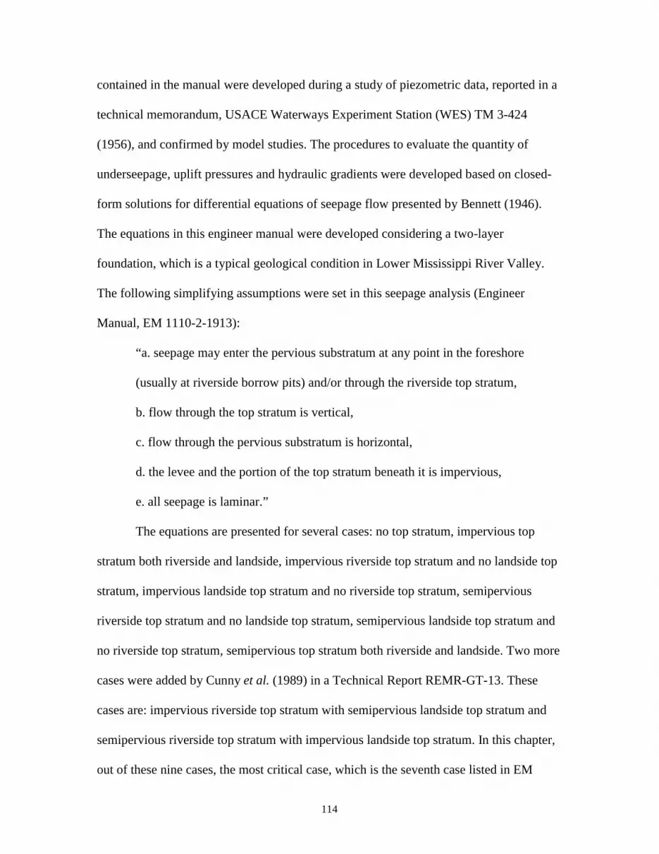
ANALYTICAL STUDY ON FLOOD INDUCED SEEPAGE UNDER RIVER LEVEES A Dissertation Submitted to Graduate Faculty of the Louisiana State University and Agricultural and Mechanical College in partial fulfillment of the requirements for the degree of Doctor of Philosophy in The Department of Civil and Environmental Engineering by Senda Ozkan B.S., Middle East Technical University, 1992 M.S., Louisiana State University, 1996 May 2003
Transcript
ANALYTICAL STUDY ON FLOOD INDUCED SEEPAGE UNDER RIVER LEVEES
A Dissertation
Submitted to Graduate Faculty of the Louisiana State University and
Agricultural and Mechanical College in partial fulfillment of the
requirements for the degree of Doctor of Philosophy
in
The Department of Civil and Environmental Engineering
by
Senda Ozkan B.S., Middle East Technical University, 1992
M.S., Louisiana State University, 1996 May 2003
ii
ACKNOWLEDGMENTS
I am very thankful to my main advisor, Dr. Dean Adrian. He always showed his
full trust, encouragement and support to my efforts. With his vast guidance, I have
experienced the joy of applied mathematics in my research. My appreciation also extends
to my dissertation committee, Dr. Vijay Singh, Dr. Roger Seals, Dr. Mehmet Tumay and
Dr. Nan Walker for their valuable guidance.
I would like to thank the U.S. Army Corps of Engineers (USACE) for funding
this project through contract DACW39-99-C-0028, and Mr. George Sills, USACE
Vicksburg District, who first suggested this research idea. I thank the support and
understanding of my friends, co-workers, and my managers at Gulf Engineers and
Consultants (GEC), Inc. I also thank Mr. William Luellen for his editorial reviews.
I want to acknowledge Ms. Joan Adrian for her continuous support to my family.
The Adrians became my second parents in the U.S.
My special thanks go to my spouse, Ahmet who has supported me through all of
my graduate studies. He has encouraged me and tried to make contributions at every step
of my research. I also owe a lot to my parents and brothers for their inspiration and
encouragement. And my very special thanks go to my little boy, Toros. I wouldn’t finish
this research without his love, joy and cheers.
iii
TABLE OF CONTENTS ACKNOWLEDGMENTS .................................................................................................. ii ABSTRACT .....................................................................................................................v CHAPTER 1 INTRODUCTION .......................................................................................1 1.1 Objectives ................................................................................................................5 1.2 Outline of Dissertation.............................................................................................6 1.2 Scope of Study .........................................................................................................7 CHAPTER 2 BACKGROUND AND LITERATURE REVIEW..........................................10 2.1 Introduction ...........................................................................................................10 2.2 Seepage Erosion ....................................................................................................10 2.3 Development of Underseepage and Sand Boils ....................................................14
2.3.1 Field Observations of Underseepage and Sand Boils ................................15 2.3.2 Soil Properties Susceptible to Piping ........................................................20
2.4 Geology of Lower Mississippi River Valley and Its Influence on Levee Underseepage ........................................................................................................21
2.5 Previous Studies on Levee Underseepage Conducted by USACE........................27 2.6 Current Underseepage Analysis Methods..............................................................31 2.7 Analytical Studies on Transient Flow....................................................................32 2.8 Cumulative Effects.................................................................................................37 2.9 Summary and Concluding Remarks ......................................................................39 2.10 List of Symbols and Acronyms..............................................................................40 CHAPTER 3 TRANSIENT FLOW MODEL IN A CONFINED AQUIFER .................42 3.1 Introduction............................................................................................................42 3.2 Analytical Modeling of Transient Hydraulic Head in a Confined Aquifer by
Laplace Transform Method....................................................................................43 3.3 Analytical Modeling of Transient Hydraulic Head in a Confined Aquifer by an
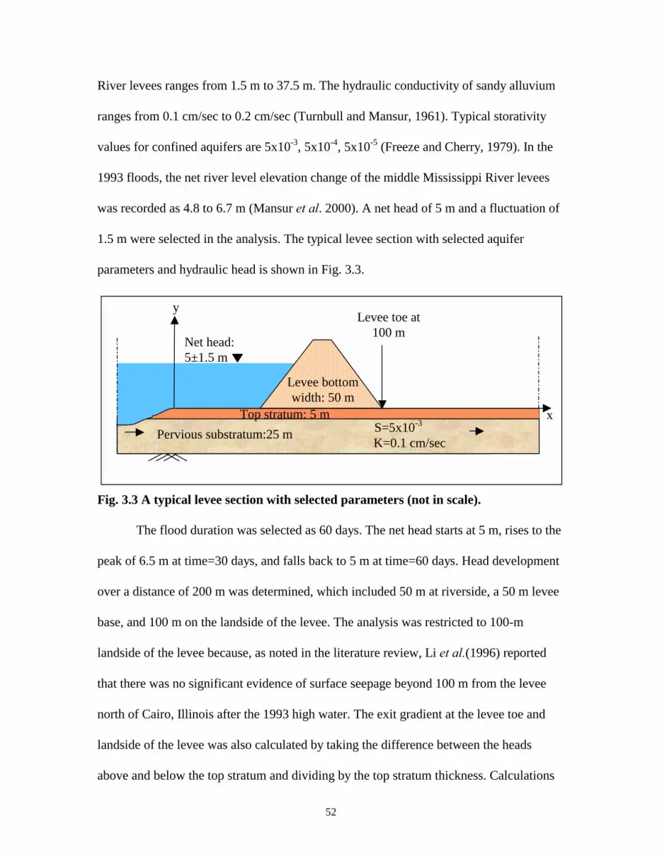
Approximate Method.............................................................................................49 3.4 Results and Discussion ..........................................................................................51 3.5 Summary................................................................................................................60 3.6 List of Symbols ......................................................................................................61 CHAPTER 4 TRANSIENT FLOW MODEL WITH LEAKAGE OUT OF A
CONFINED AQUIFER.............................................................................64 4.1 Introduction............................................................................................................64 4.2 Analytical Modeling of Transient Hydraulic Head with Leakage Out of a
Confined Aquifer by Laplace Transform Method .................................................64 4.3 Analytical Modeling of Transient Hydraulic Head with Leakage Out of a
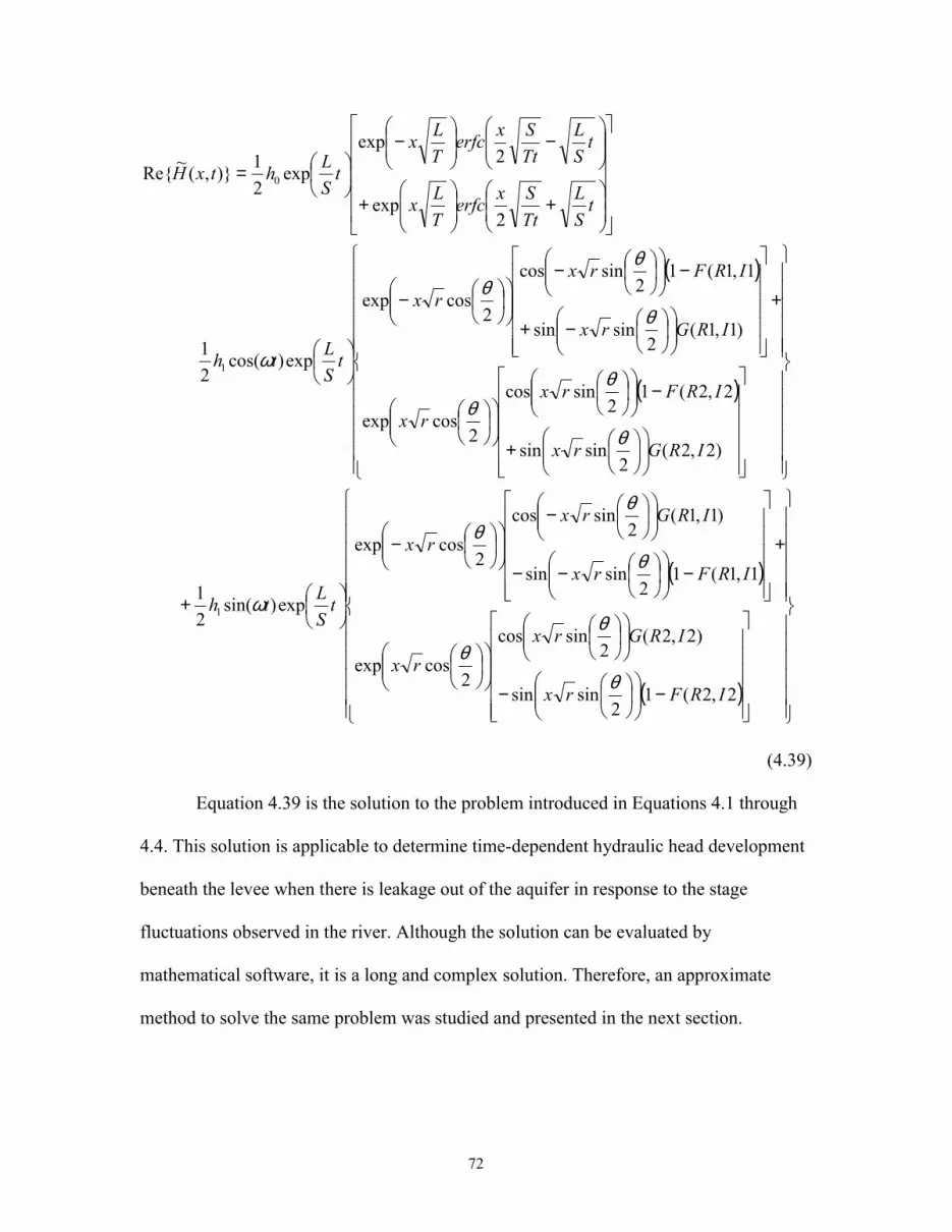
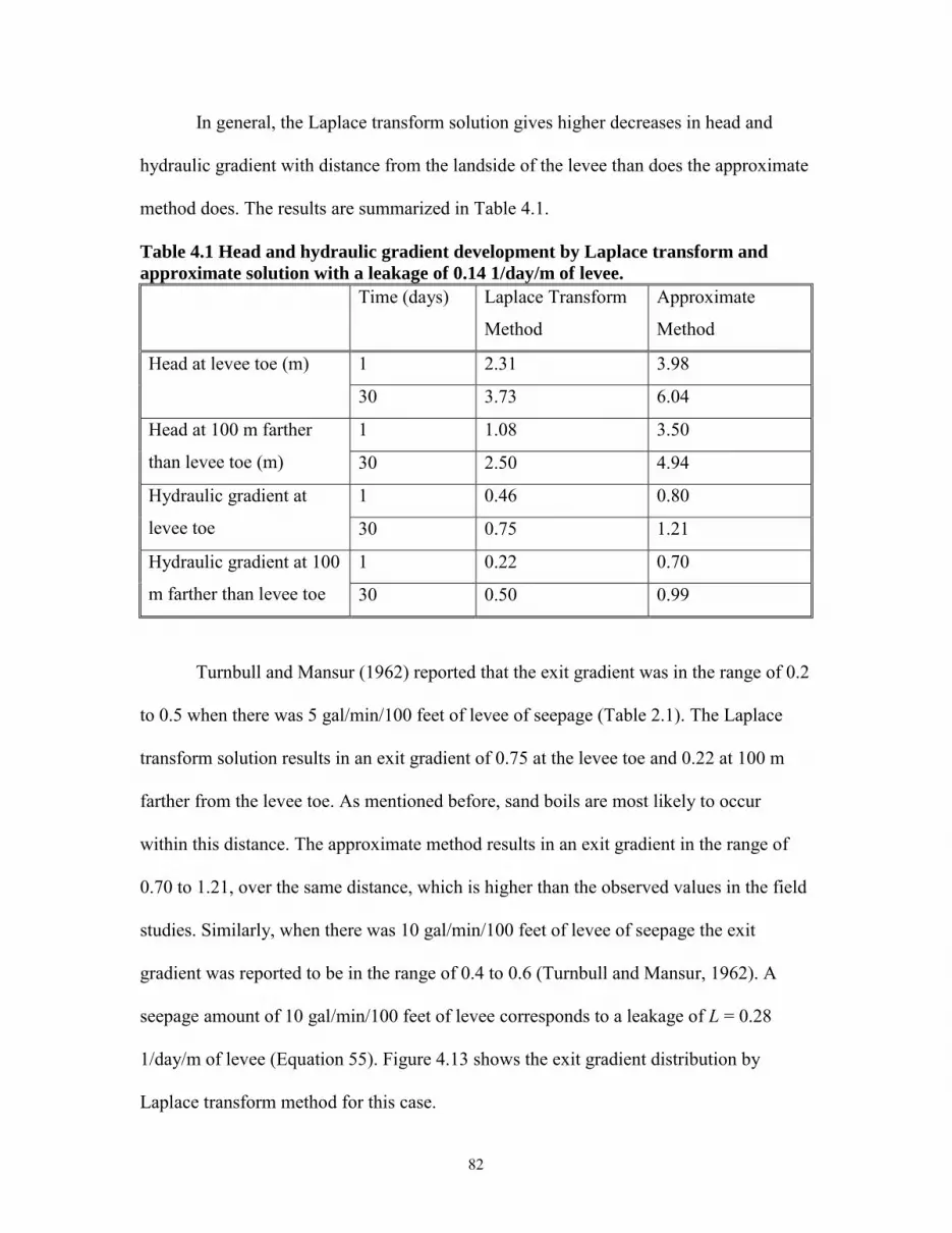
Confined Aquifer by an Approximate Method......................................................73 4.4 Results and Discussion ..........................................................................................75 4.5 Summary................................................................................................................90 4.6 List of Symbols ......................................................................................................91
iv
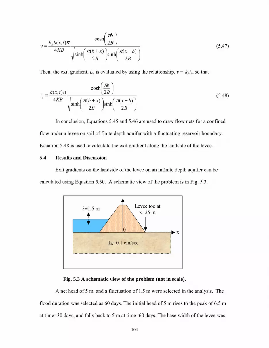
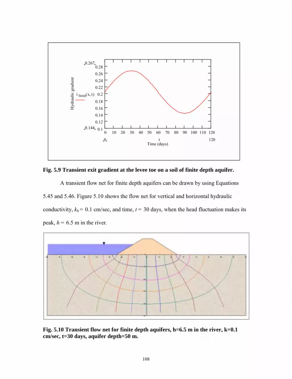
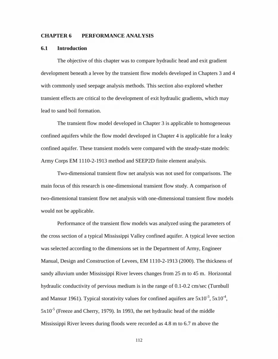
CHAPTER 5 CONSTRUCTION OF TRANSIENT FLOW NETS................................94 5.1 Introduction............................................................................................................94 5.2 Construction of Transient Flow Nets for Infinite Depth Aquifers........................95 5.3 Construction of Transient Flow Nets for Finite Depth Aquifers ........................100 5.4 Results and Discussion ........................................................................................104 5.5 Summary..............................................................................................................109 5.6 List of Symbols ....................................................................................................109 CHAPTER 6 PERFORMANCE ANALYSIS ...............................................................112 6.1 Introduction..........................................................................................................112 6.2 Performance Analysis of Transient Flow Model in a Confined Aquifer.............117 6.3 Performance Analysis Transient Flow Model with Leakage Out of a
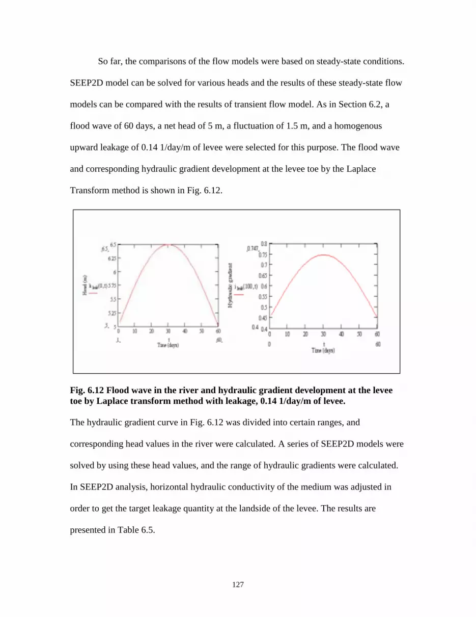
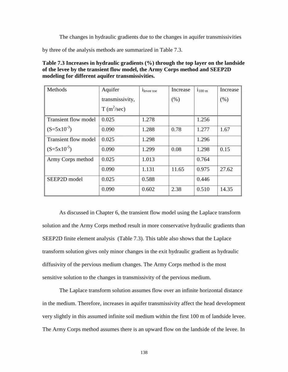
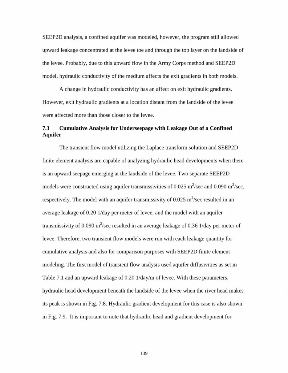
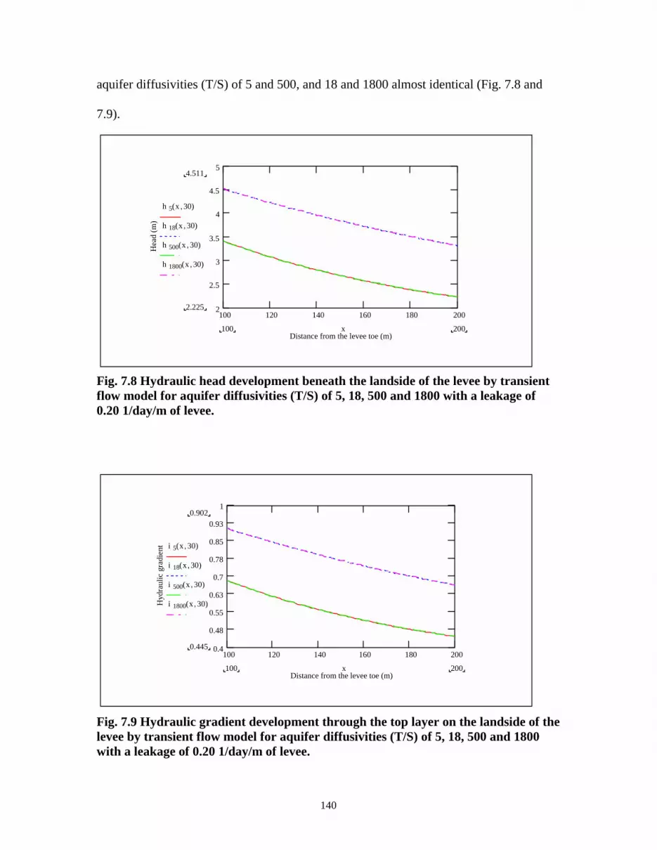
ConfinedAquifer ..................................................................................................123 6.4 Summary and Conclusions ..................................................................................128 6.5 List of Symbols ....................................................................................................130 CHAPTER 7 EVALUATION OF CUMULATIVE EFFECTS ....................................131 7.1 Introduction..........................................................................................................131 7.2 Cumulative Analysis for Underseepage in a Confined Aquifer ..........................133 7.3 Cumulative Analysis for Underseepage with Leakage Out of a Confined
Aquifer .................................................................................................................139 7.4 Summary and Conclusions ..................................................................................147 CHAPTER 8 CONCLUDING REMARKS...................................................................149 REFERENCES ................................................................................................................153 APPENDIX A CALCULATIONS AND GRAPHS IN CHAPTER 3 AND 4 ..........160 APPENDIX B CALCULATIONS AND GRAPHS IN CHAPTER 5 .......................174 APPENDIX C CALCULATIONS AND GRAPHS IN CHAPTER 6 .......................180 APPENDIX D CALCULATIONS AND GRAPHS IN CHAPTER 7 .......................199 VITA ..............................................................................................................................241
v
ABSTRACT A common and potentially dangerous phenomenon associated with flooding is
seepage under levees and the formation of sand boils. Seepage flow due to hydrostatic
head gradients of floods may cause deformation of pervious layers leading to heave,
piping and sand boils. Underseepage may also cause irreversible changes in the
characteristics of the porous medium. A series of independent flood events may have
cumulative effects on pervious layers causing sand boils to grow. Current underseepage
analyses for levees are based on steady-state flow. Transient seepage flow due to rapid
changes in river head may contribute to cumulative effects and cause critical hydraulic
head development under levees and subsequent sand boil formation.
This research examined transient effects on hydraulic head development under
levees during a flood event. While the research is focused on levees, this study is
applicable to any hydraulic structures (e.g., flood walls, dams, and retaining structures)
subject to underseepage. An analytical model was developed for one-dimensional
transient flow in a confined aquifer under a levee in response to river stage fluctuations.
This analytical model was revised by considering leakage out of confined aquifers to
simulate the occurrence of sand boils on the landside of levees. Transient flow nets were
also constructed using complex variables. The performance of these analytical models
was evaluated by comparing with the limited field studies, current U.S. Army Corps of
Engineers underseepage analysis methodology for levees, and a finite element program.
The effects of possible cumulative deformations on development of exit hydraulic
gradients were also evaluated and discussed.
Transient flow models performed reasonably well compared with the limited field
studies, the Army Corps seepage analysis method and SEEP2D finite element program.
vi
Cumulative analysis of underseepage by the transient flow model simulating sand boil
formations showed significant increases in exit hydraulic gradients in response to
possible cumulative changes in aquifer characteristics.
1
CHAPTER 1 INTRODUCTION
Underseepage of water through soil below levees during times of flood is a
natural phenomenon. Seepage becomes a matter of concern for the safety of a levee when
piping occurs and sand boils form. Turnbull and Mansur (1961) summarized the flood
induced seepage problem under levees based on their experience with the U.S. Army
Corps of Engineers (USACE). If the hydrostatic pressure force in the pervious substratum
landward of the levee becomes greater than the submerged weight of the overlying strata,
the excess pressure may cause heaving of the upper soil layers and rupture at weak spots
with a resulting concentration of seepage flow. Flow from these weakened locations may
increase to form sand boils. In addition, the concentrated seepage flow may erode fine
soil particles, and carry these fine particles up to the surface. As the erosion process
continues, a pipe or open channel may form through the top stratum. The pipe-shaped
opening through which water and eroded soil discharge is called a sand boil. A sand boil
opening bears some resemblance to a soil-walled pipe through the top stratum. The
flowing water exiting through a sand boil carries soil particles that have been eroded from
along the water’s seepage path up to the soil surface where it may deposit to form a cone
around the sand boil. Heave and piping are the main mechanisms involved in creating a
pipe that leads to sand boils. Heaving occurs when seepage forces push the substrata
upward. Piping is the phenomenon where seeping water progressively erodes and washes
away soil particles, leaving large voids in the soil. Removal of soil through sand boils by
piping or internal erosion damages levees, their foundations, or both, which may result in
settlement and has the potential to cause catastrophic failures of levees. A schematic view
of the underseepage problem is shown in Fig. 1.1.
2
Fig. 1.1 A schematic representation of seepage problem under levees (U: hydrostatic uplift pressures, W: submerged weight of soil).
Although an exit hydraulic gradient of 0.85 on the landside of a levee is
commonly considered sufficient to initiate sand boil formation, other field measurements
show that sand boils may occur with exit hydraulic gradients in the range of 0.54 -1.02
(Daniel, 1985). A photo of a sand boil in shown Fig. 1.2
While most analyses of underseepage, piping, heaving, and sand boil formation
have been based on steady seepage flow, it is unsteady seepage flow that is more
common for canal embankments and levees (Peter, 1982). This is because during floods
the water level in the river and between the levees changes so quickly that a constant flow
regime is unlikely to be established. Instead, rapid changes of water level may cause a
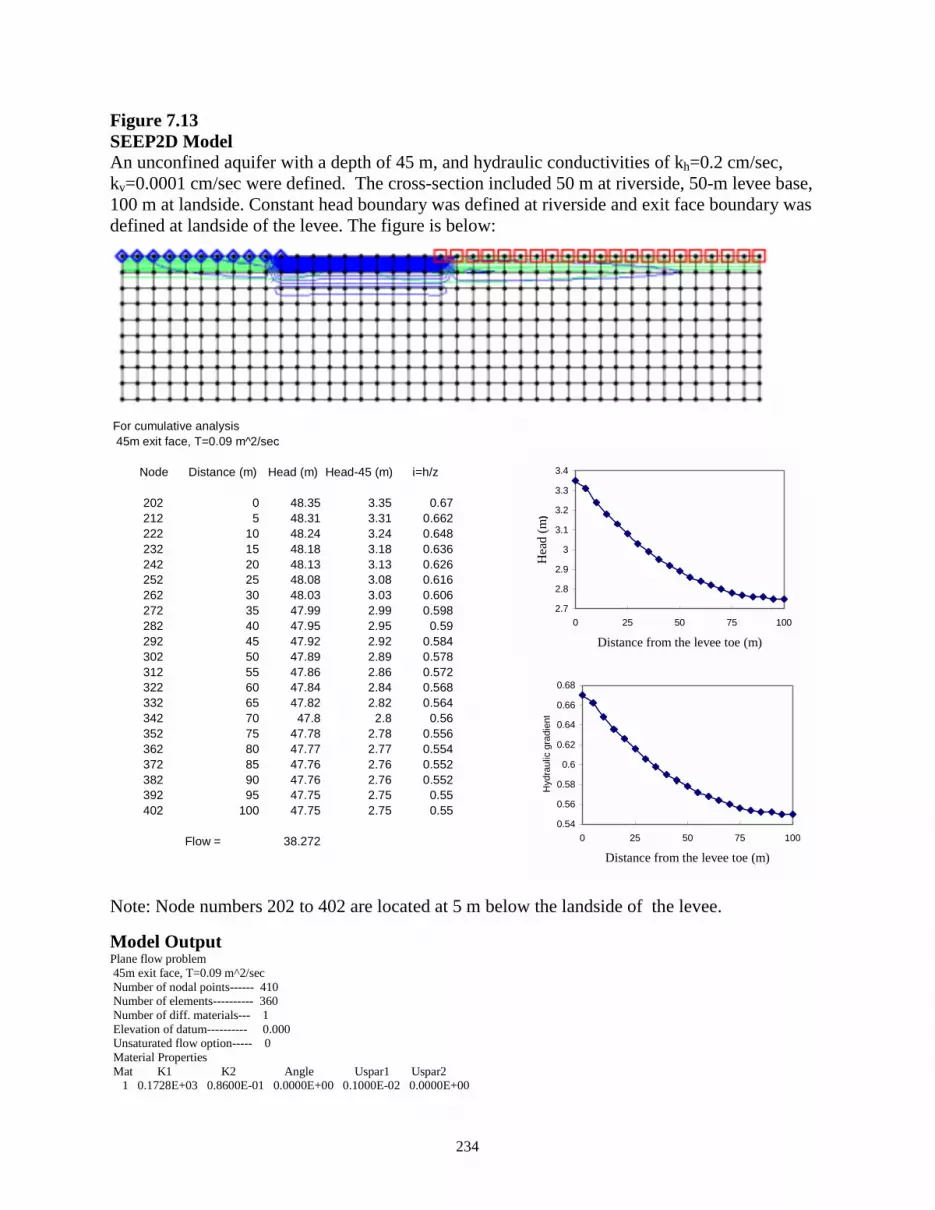
head wave moving with varying velocity in the stratified porous medium. Consider that a
levee is underlain with a layer of high hydraulic conductivity soil, which extends a
distance on the landside of the levee, while a layer of low hydraulic conductivity soil
overlies the high conductivity layer on the landside of the levee (Fig. 1.3).
Top stratum
Leveesand boil
heave, piping
Flooded river
fine particle erosion and
pipe formation
seepage flow
U
W
3
Fig. 1.2 A picture of a sand boil (source: USACE, Vicksburg District).
Fig 1.3 A hydraulic structure and seepage forces acting on sand and gravel layer in its subsoil (after Peter, 1982). When a flood wave occurs in the layer of greater hydraulic conductivity, the head wave
reaches farther in a given time than it does in the top layer. As the head wave develops,
so do uplift pressures that may induce heave and gradual liquefaction of the overlying
4
layer. Static liquefaction is a soil state at which vertical effective stress on soil becomes
zero (Fig. 1.1). A mass of sand in a state of static liquefaction is known as quicksand,
which has lost its strength and behaves like viscous liquid (Budhu, 2000).
If the same problem were to be analyzed as a steady state problem, then the upper
layer would be assumed to be wet and thus heavier than similar dry material, so the heave
would have been less likely to occur. However, steady seepage is frequently assumed in
analyses of levees because the computations are simpler and the steady-state seepage
parameters are less difficult to determine than the corresponding transient parameters
(Peter, 1982). For these reasons, seepage flow based on transient effects due to changes
in river head has not been analyzed in as much detail as has steady flow.
At one time, it was thought that sand boils could “heal” or “repair” themselves
between flood events (Sills, G., personal communication to CE 7265 class, Fall 1997).
After the 1993 floods on the Upper Mississippi River, some engineers with the U.S.
Army Corps of Engineers began to question the extent of the inter-flood healing effect
and whether there is a cumulative effect caused by sand boils. (Sills, G., personal
communication to CE 7265 class, Fall 1997).
A more recent concept is that seepage under levees during a series of independent
flood events may cause sand boils to grow as the flood series grows longer. Researchers
have not examined the concept that there may be cumulative effects from sand boils,
which increase the likelihood of levee failure due to seepage. As a result, the problem of
levee failure due to cumulative effects of underseepage is only now being recognized as a
problem that may have great urgency for evaluating the danger to lives and property in
areas protected by levee systems. Currently, the USACE Engineer Research and
Development Center (ERDC) in Vicksburg, Mississippi, is working on research on the
5
cumulative effects of piping under levees (Wolff, 2002). The research unit operates under
the Innovative Flood Damage Research Program (IFDR) sponsored by USACE.
1.1 Objectives
The objective of this research was to obtain a better understanding of the sand boil
problem. This dissertation explored the following two questions: (1) Is transient flow
analysis due to river head fluctuations critical in the development of exit hydraulic
gradients and the subsequent sand boil formation? and (2) If sand boils develop more
frequently due to cumulative effects associated with repetitive flood events, how can
transient flow analysis in conjunction with current underseepage analysis tools respond to
this problem? Both questions were addressed by developing transient flow models and
comparing them with current underseepage analysis tools. The transient flow models
developed in this study are also expected to contribute to the current literature on
analytical techniques for seepage problems. The following specific objectives were
established for this study:
1. develop an analytical model to describe hydraulic head in response to river head
fluctuations in a confined aquifer under a levee,
2. develop an analytical model to describe hydraulic head in response to river head
fluctuations under a levee with leakage out of a confined aquifer,
3. construct time-dependent flow nets for underseepage analysis,
4. evaluate the performance of these analytical models by comparing them with other
current practice underseepage analysis methods, and
5. evaluate possible cumulative effects in hydraulic head development with new
analytical models and other underseepage analysis methods.
6
1.2 Outline of Dissertation
The dissertation is organized as follows: This chapter gives an introduction to the
research, an outline of the problem, the main questions asked, and the specific objectives
of the study.
The second chapter gives background information and literature review. It
provides detailed information on seepage erosion, previous studies on underseepage of
levees conducted by USACE, current underseepage analysis tools, analytical studies on
transient flow, and possible cumulative effects due to repetitive flood events.
The third and fourth chapters present transient analytical hydraulic head models;
for a confined aquifer in the third chapter and with leakage out of a confined aquifer in
the fourth chapter. In both, a solution with Laplace transform method and an approximate
solution are presented. The fifth chapter details analytical construction of transient flow
nets for infinite-depth aquifers and finite-depth aquifers. The results and a discussion
about the transient models and flow nets are given in each chapter.
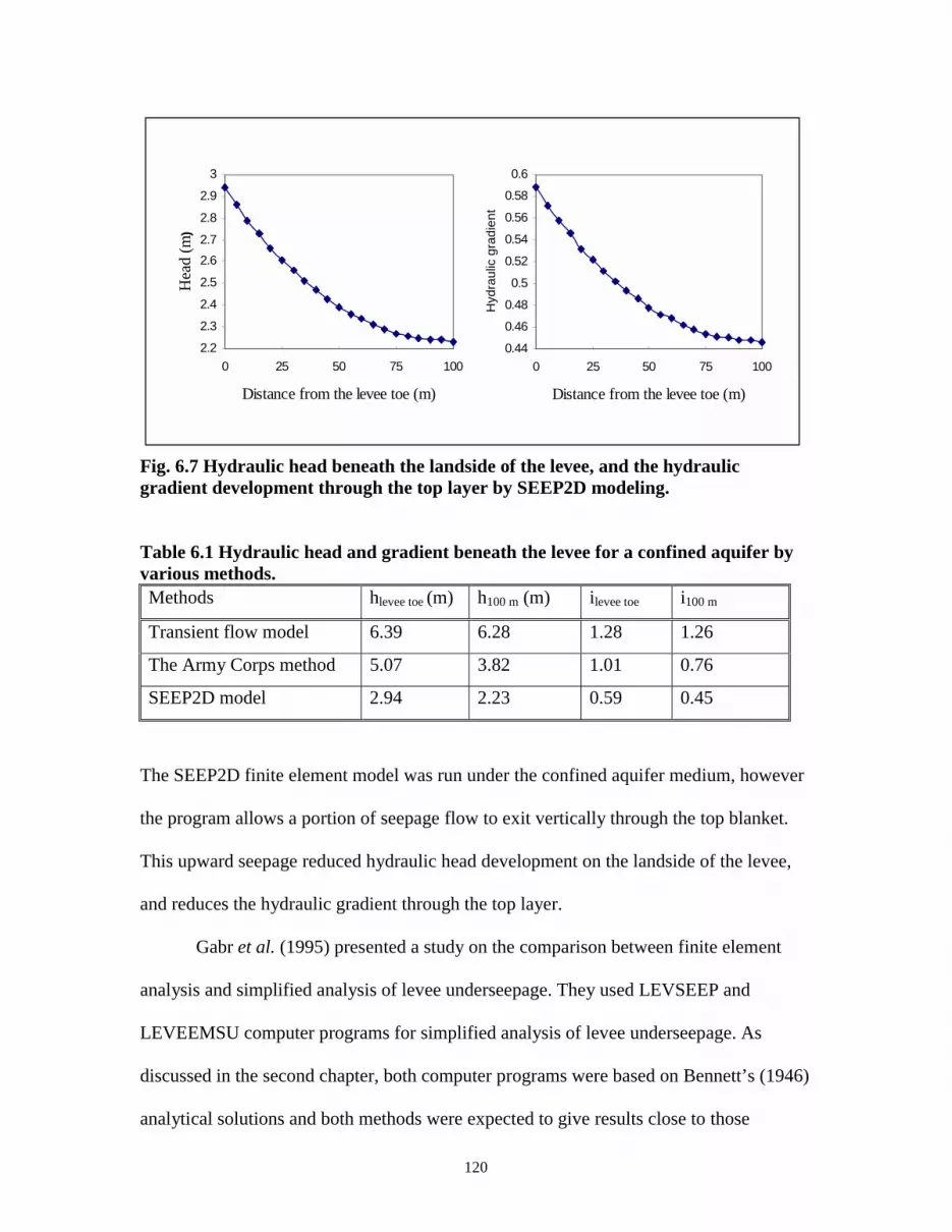
The sixth chapter provides a performance analysis of the developed models
conducted by comparing the results of the analytical models with the USACE levee
underseepage method and a finite element program. Results and discussion of this section
explore the main question of this study: whether transient effects are critical in
development of exit hydraulic gradients, which may trigger sand boil formation.
Cumulative effects due to repetitive flood events are discussed in the seventh
chapter and are evaluated by transient flow models, USACE levee underseepage method,
and a finite element program. The results and discussion of these evaluations explore the
second question of this study: how transient flow analysis and current underseepage
7
analysis tools respond to possible cumulative effects due to repetitive flood events. The
conclusions are presented in the eighth chapter.
There are four appendices containing details of mathematical computations and
finite element models.
1.3 Scope of Study
This research involved the use of mathematical models, which were supplemented
by data from published on-site investigations.
Typical geological features of Mississippi River Valley include a less permeable
top stratum and a more pervious substratum. This geological feature may allows us to do
confined flow analysis. In the analytical models, linear laws of seepage were studied,
where there is a linear relationship between seepage velocity and hydraulic gradient. The
pervious substratum typically combines horizontally stratified beds of sand where
horizontal conductivity of the main aquifer is so large compared to hydraulic conductivity
of the semi-pervious top stratum. Therefore, it is safe to assume that horizontal flow in
the pervious substratum is refracted over 900 to seep vertically through the semi-
confining layer due to hydraulic uplift forces (Hantush and Jacob, 1955). While, all
groundwater flow in nature is three-dimensional to a certain extent, symmetry features,
i.e. flow to a well, make the problem possible to analyze in two-dimensional form (De
Wiest, 1965). The solution may need to be further simplified by reducing the
dimensionality of the problem to one due to difficult boundary conditions. Reducing the
dimensionality of the problem introduce significant errors and it is up to hydrologists’
judgement to estimate the error in engineering practice. In the light of this discussion,
certain simplifications were applied in the development of analytical models in this
research.
8
The analytical models for transient flow in a confined aquifer were developed by
using the diffusion equation, which was derived under Darcy’s law, and the law of
conservation of mass. The geologic conditions beneath the levees can be very complex.
To simplify the problem the stratum was assumed as saturated, homogenous, and
isotropic, and the flow is assumed as one-dimensional. Transient analytical flow models
with leakage out of a confined aquifer were presented and a subsurface system with a
leaky confined aquifer and a semi-permeable layer on the top of it was considered. The
assumptions introduced by Hantush and Jacob (1955) on leaky aquifer systems - that
storage in the semi-permeable layer is negligible and the leakage is linearly proportional
to the difference in head between two layers - are applicable here.
The methodologies given by Polubarinova-Kochina (1962) were followed for
transient analytical flow nets for infinite and finite depth aquifers. The assumptions and
the conditions in her solutions were maintained. A downward vertical flow at the
riverside of the levee, a horizontal flow under the levee and an upward vertical flow at
the landside of levee were assumed. The solution is for homogenous and isotropic soil
conditions.
The performance of the analytical models was compared with the other seepage
analysis tools. Even though a simple cross-section with typical soil parameters was used,
the comparisons may not reflect identical conditions as each method was developed
under its own assumptions. The transient flow models and other seepage analysis tools
were used to evaluate possible cumulative effects of flood-induced seepage. As explained
in the literature survey, there is a distinct lack of published studies on cumulative effects
of underseepage problems associated with sand boils. The best evaluation of cumulative
effects can be conducted by examining data from long-term site investigations and by
9
conducting laboratory experiments. The evaluation of cumulative effects by empirical,
analytical and numerical methods is complicated. The transient analytical models
developed in this study attempt to provide a view to the problem of evaluating cumulative
effects of sand boils. Further research is needed in this area.
10
CHAPTER 2 BACKGROUND AND LITERATURE REVIEW
2.1 Introduction
The following items are reviewed in this chapter: seepage erosion mechanisms;
levee underseepage and sand boil formation; field observations; soil properties
susceptible to piping problem; geology of Lower Mississippi River Valley and its
influence on underseepage; previous studies on levee underseepage conducted by
USACE; current underseepage analysis methods; analytical studies on transient flow with
cyclical boundary conditions; and cumulative effects. A list of symbols is included at the
end of the chapter.
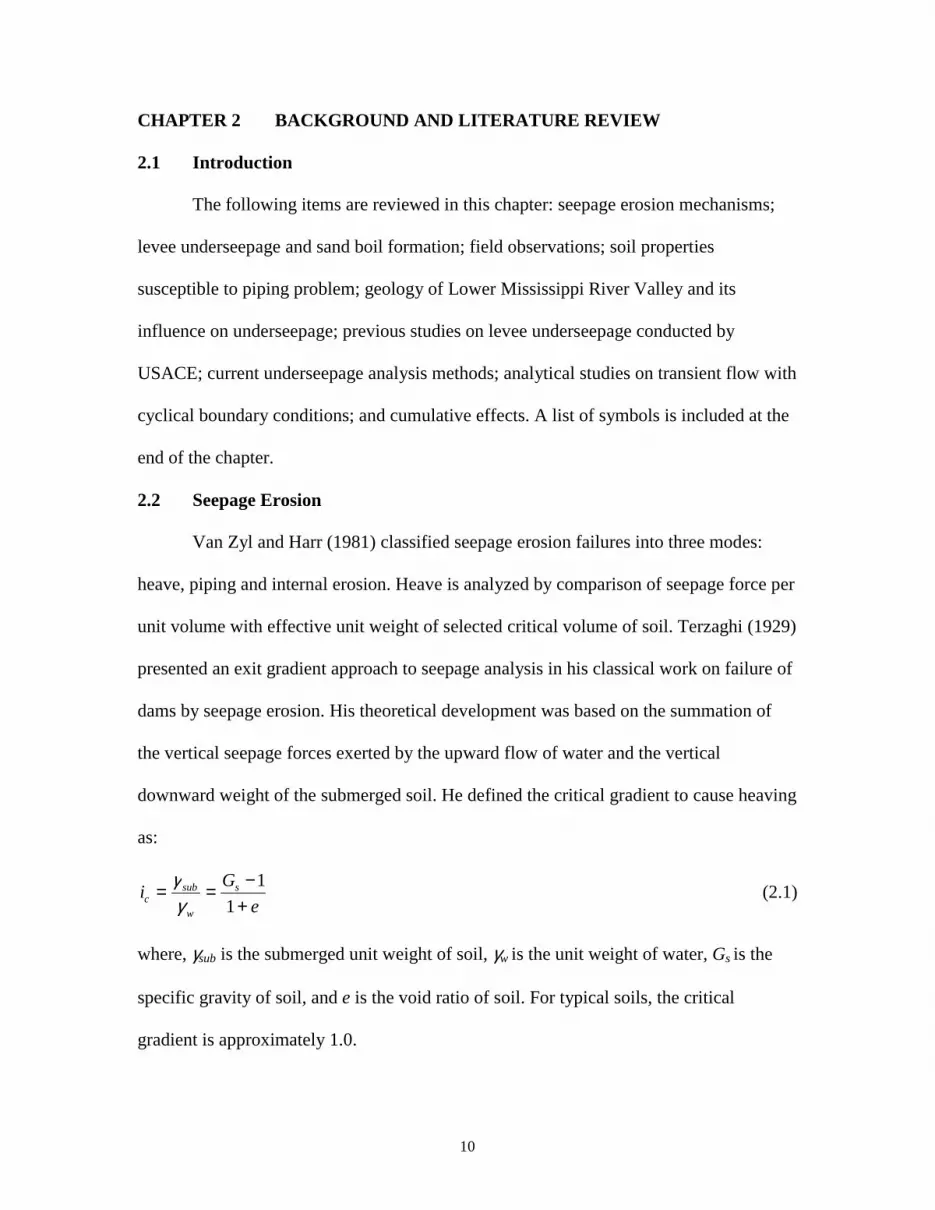
2.2 Seepage Erosion
Van Zyl and Harr (1981) classified seepage erosion failures into three modes:
heave, piping and internal erosion. Heave is analyzed by comparison of seepage force per
unit volume with effective unit weight of selected critical volume of soil. Terzaghi (1929)
presented an exit gradient approach to seepage analysis in his classical work on failure of
dams by seepage erosion. His theoretical development was based on the summation of
the vertical seepage forces exerted by the upward flow of water and the vertical
downward weight of the submerged soil. He defined the critical gradient to cause heaving
as:
eGi s
w
subc +
−==1
1γγ (2.1)
where, γsub is the submerged unit weight of soil, γw is the unit weight of water, Gs is the
specific gravity of soil, and e is the void ratio of soil. For typical soils, the critical
gradient is approximately 1.0.
11
Sherard et al. (1963) investigated the mechanics of piping in earth and earth-rock
dams. As water flows, the pressure head is dissipated in overcoming viscous drag forces,
which resist the flow through the small pores. The seeping water also generates erosive
forces and tends to drag the soil particles with it as it travels through the pervious layer. If
the seepage erosive forces are greater than the erosion resisting forces, the soil particles
are washed away and piping starts. If the soil has some cohesion, a small tunnel or pipe
can form at the downstream exit face of a seepage path. Once piping starts, the flow in
the pipe increases due to the decreased resistance to flow, piping accelerates, and the
small tunnel or pipe lengthens. Van Zyl and Harr (1981) stated that the analysis of piping
erosion was almost impossible due to control by discontinuities. However, global
gradient approaches developed by Bligh (1927) and Lane (1935) are still widely used in
the design of dams and weirs. The concept of the length of the path traveled by seeping
water led to the development of creep ratios or creep coefficients. Bligh (1927) defined a
creep coefficient as:
hLC = (2.2)
where L is the length of seepage path measured along the base of weir, and h is the total
head loss. Lane (1935) suggested a weighted creep ratio as:
h
LL
Cv
h
w
+= 3 (2.3)
where, Lh is distance along horizontal contacts (<450, measured from the horizontal), Lv is
distance along vertical contacts (>450) and h is total head loss. Bligh (1927) and Lane
(1935) suggested limiting values for creep coefficients obtained by analyzing a large
number of structures founded on various soil conditions. Some typical values of weighted
12
creep ratio are: 8.5 to 5.0 for very fine sand to coarse sand, 4.0 to 2.5 for fine gravel to
boulders, and 1.8 for hard clay (Lane, 1935).
Internal erosion begins locally by fine particles being moved from the soil matrix
into a coarser layer leading to formation of cavities, collapse and failure. The mechanism
is an important concern for the analysis of seepage through the hydraulic structures in the
event of transfer of particles between zones of earth and rock-fill dams, and in dispersive
soils (Sherard et al., 1972). While the analysis of internal erosion is generally very
difficult, installation of filters designed to proper filter criteria is the common prevention
technique (Van Zyl and Harr, 1981).
Casagrande (1937) estimated the exit gradient from flow nets. Khosla et al.
(1936) and Harr (1962) suggested theoretical methods to determine the exit gradients for
confined flow for specific cross-sections. Khilar et al. (1985) investigated the potential
for clay soils to pipe or plug under induced flow gradients. They presented the following
equation as a measure of the critical gradient to cause piping:
2/1
0
0
878.2
=
kn
iw
cc γ
τ (2.4)
where τc is the critical tractive shear stress (dynes/cm2), n0 is the initial porosity, and k0 is
the initial intrinsic permeability (a typical value is, k0 = 10-10 cm2). For granular materials,
critical tractive shear stress can be estimated from the d50 size (Lane, 1935) as
τc (dynes/cm2) = 10d50 (mm). Aralunandan and Perry (1983) studied the erodibilty of
core materials in earth and rock dams. They reported that the erosion resistant soils have
a critical tractive shear stress of τc ≥ 9 dynes/cm2 based on limited data.
Soil type, rate of head increase and the flow condition are the main dependents for
modes of seepage erosion failure (Van Zyl and Harr, 1981). The soil type controls
13
whether heave is followed by a quick condition as in clean sand or whether heave leads to
crack formation, concentrated flow and piping. Heave, leading to cracks, concentrated
flow and piping, appears to be more common in granular soils with a large percentage of
fines.
A rapid increase in head may result in heave of the surface, leading to a quick
condition (Van Zyl and Harr, 1981). This could be a typical failure condition on the
downstream side of a water retention structure being filled rapidly. A quick condition
before heave can also be produced when the head is raised very slowly. Tomlinson and
Vaid (2000) presented an experimental study of piping erosion. They tested various
artificial granular filter and base soil combinations in a permeameter under variable
confining pressures to determine the critical gradient where soil erodes through the filter.
They observed that the critical gradient was lower if the head was rapidly increased. Van
Zyl and Harr (1981) also pointed out the importance of flow conditions in piping
problems. According to the field observations, an unsaturated soil fails at lower gradients
than the critical gradient of the soil. The first filling of a reservoir may induce this type of
failure.
Sellmeijer and Koenders (1991) stated that empirically, a so-called piping channel
or slit develops, extending from the downstream corner of the structure to a length of less
than half the bottom length of a dam. They presented a mathematical model for piping.
They modeled a prediction of an equilibrium situation in which some materials have
washed away from underneath the structure and the channel development has stopped.
The result of this study was a mathematical representation of the relation between the
pipe length and the difference in water head. Ojha et al. (2001) developed a piping model
based on Darcy’s law. They concluded that the choice of permeability function was
14
critical for the piping model. The permeability functions, which depend only on grain
size, have limited value on clarifying piping models while those that include porosity are
more useful.
2.3 Development of Underseepage and Sand Boils
Turnbull and Mansur (1961) explained underseepage mechanisms and sand boil
formation at Mississippi River levees as a result of the studies and investigations
conducted by the Army Corps of Engineers covering a period of 1937 to 1952:
“Whenever a levee is subjected to a differential hydrostatic head of water as a result of river stages higher than the surrounding land, seepage enters the pervious substratum through the bed of the river and riverside borrow pits or the riverside top stratum or both, and creates an artesian head and hydraulic gradient in the sand stratum under the levee. This gradient causes a flow of seepage beneath the levee and the development of excess pressures landward thereof. If the hydrostatic pressure in the pervious substratum landward of the levee becomes greater than the submerged weight of the top stratum, the excess pressure will cause heaving of the top blanket, or will cause it to rupture at one or more weak spots with a resulting concentration of seepage flow in the form of sand boils.
“In nature, seepage usually concentrates along the landside toe of the levee, at thin or weak spots in the top stratum, and adjacent to clay-filled swales or channels. Where seepage is concentrated to the extent that turbulent flow is created, the flow will cause erosion in the top stratum and development of a channel down into the underlying silts and fine sands, which frequently exist immediately beneath the top stratum. As the channel increases in size or length, or both, a progressively greater concentration of seepage flows into it with a consequent greater tendency for erosion to progress beneath the levee.
“The amount of seepage and uplift hydrostatic pressure that may develop landward of a levee is related to the river stage, location of seepage entrance, thickness and perviousness of the substratum and of the landside top stratum, underground storage, and geological features. Other factors contributing to the activity of the sand boils caused by seepage and hydrostatic pressure are the degree of seepage concentration and the velocity of flow emerging from the boils.”
Turnbull and Mansur (1961) also explained the importance of underground
storage on underseepage and excess hydrostatic pressure during relatively low high
waters and high waters of short duration. They noted that during a high water, if the
ground water table is low, drainage into subsurface storage landward of the levee reduces
15
hydrostatic pressures and seepage rising to the surface. However, if the ground water
table is high or the flood is of long duration, this factor has little effect on substratum
hydrostatic pressures. In general, piezometric data obtained during the 1950 high water
indicated that ground water storage landward of the levees was filled by the time a high
flood stage developed.
The critical gradient required to cause sand boils or heaving is estimated by
Equation 2.1. Approximate theoretical critical gradients for silty sands and silts is
approximately 0.85 and for silty clay and clay is 0.80 (Turnbull and Mansur, 1961). In
the field, the critical gradient required to cause sand boils can best be determined by
measuring the hydrostatic head beneath the top stratum at the time a sand boil starts. The
critical gradient in the field is determined by
t
xc z
hi = (2.5)
where hx is the head beneath top stratum at distance x landward from landside toe of the
levee, and zt is the thickness of landside top stratum.
2.3.1 Field Observations of Underseepage and Sand Boils
Mansur, et al. (2000) reviewed studies carried out since the 1940's on
underseepage, piping, and sand boil formation in the Mississippi River Valley. The
Mississippi River floods of 1993 produced seepage under some levees which resulted in
dramatic levee failures in the Kaskasia Island Levee District in Illinois (Mansur, et al.,
2000). A sand boil and subsurface piping caused the Kaskasia Island levee to fail,
flooding the entire levee district.
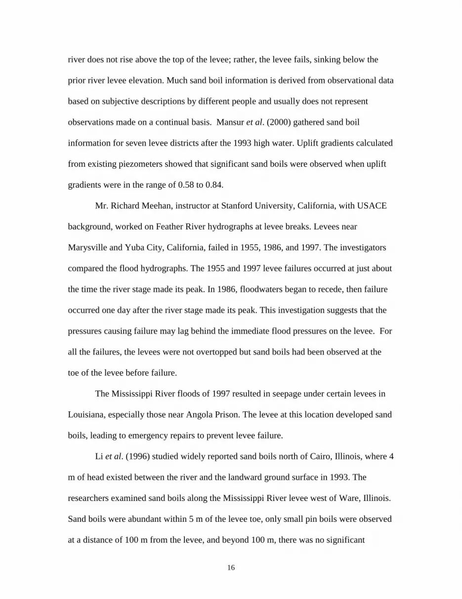
According to witnesses, levee failures due to high water usually starts with sand
boil occurrences near the toe of the levee, followed by overtopping. In some cases, the
16
river does not rise above the top of the levee; rather, the levee fails, sinking below the
prior river levee elevation. Much sand boil information is derived from observational data
based on subjective descriptions by different people and usually does not represent
observations made on a continual basis. Mansur et al. (2000) gathered sand boil
information for seven levee districts after the 1993 high water. Uplift gradients calculated
from existing piezometers showed that significant sand boils were observed when uplift
gradients were in the range of 0.58 to 0.84.
Mr. Richard Meehan, instructor at Stanford University, California, with USACE
background, worked on Feather River hydrographs at levee breaks. Levees near
Marysville and Yuba City, California, failed in 1955, 1986, and 1997. The investigators
compared the flood hydrographs. The 1955 and 1997 levee failures occurred at just about
the time the river stage made its peak. In 1986, floodwaters began to recede, then failure
occurred one day after the river stage made its peak. This investigation suggests that the
pressures causing failure may lag behind the immediate flood pressures on the levee. For
all the failures, the levees were not overtopped but sand boils had been observed at the
toe of the levee before failure.
The Mississippi River floods of 1997 resulted in seepage under certain levees in
Louisiana, especially those near Angola Prison. The levee at this location developed sand
boils, leading to emergency repairs to prevent levee failure.
Li et al. (1996) studied widely reported sand boils north of Cairo, Illinois, where 4
m of head existed between the river and the landward ground surface in 1993. The
researchers examined sand boils along the Mississippi River levee west of Ware, Illinois.
Sand boils were abundant within 5 m of the levee toe, only small pin boils were observed
at a distance of 100 m from the levee, and beyond 100 m, there was no significant
17
evidence of surface seepage. Li et al. reported the sand boils had dimensions with 0.5 m
to 10 m diameter, and they commonly extended 0.3 m above the ground surface. Mansur
et al. (2000) reported the results of an underseepage and sand boil study after the 1993
high water. The dimensions of many sand boils were up to 30″ in diameter at Prairie
DuPont and Ft. Chartres Levee Districts, Illinois. At the other regions of Mississippi
River levees, many sand boils of 2″ to 12″ in diameter were observed. Another
observation of sand boils was reported by the Corps of Engineers after 1997 high water.
A sand boil with a throat of 0.45 m to 0.6 m (1.5 to 2.0 ft) in diameter was observed at
about 60 m (200 ft) from the levee at Blue Lake, Arkansas. The uncontrolled flow
resembled a large relief well and approximately 23 cu.m (30 cu.yd) of fine to medium
sand was deposited.
The U.S. Army Corps of Engineers, New Orleans District Office, conducted a
seepage study from Louisiana State University (LSU) to Duncan Point of Pontchartrain
Levee District in 1992. This study references data back to a technical manual, TM 3-424
published by USACE in 1956. During the 1937 high water, improperly backfilled seismic
shot holes near the LSU campus were attributed as being the cause for sand boils
experienced. During the 1950 high water, excess hydrostatic pressures of 12.5 to 15 ft
existed along the landside toe of the levee. This hydrostatic pressure corresponds to 75%
to 90% of the crest head in the river. Excess heads of 10 to 12 ft were also observed as far
as 0.75 mile (1.2 km) landward of the levee. During the 1950 high water, four fairly large
sand boils were observed but according to the available records they were not at the same
locations as the 1937 boils. During the 1973 high water, sand boils were observed at
fairly large distances up to 2.4 km from the levee. In 1975, a sand boil nicknamed “Big
Mamou” developed at about 1 mile (1.6 km) from the levee along the banks of Elbow
18
Bayou due to high water. During the 1983 high water, there was no flow from Big
Mamou but a new sand boil developed about 200-ft (61 m) away from it. Again in 1983,
a sand boil about 0.5 mile from the levee, which developed at LSU stadium parking lot,
was flowing clear.
In 1992, the USACE noted that the studied regions of levees have a relatively
thick soil blanket, which is sufficient to withstand high hydrostatic pressures. This fact
explains the occurrence of high hydrostatic pressures and sand boils as far as a mile from
the levee, where the soil blanket may be thinner. This study concluded that seepage
prevention methods, such as seepage berms and relief wells, protect limited areas.
Seepage berms may force seepage away from the levees, and relief wells along the
landside toe of a levee only create a “dip” in the hydrostatic gradient line.
Recent observations were also conducted at LSU Dairy Farm in July 2002 by Dr.
Dean Adrian, Professor, and Senda Ozkan and Curtis Sutherland, graduate students at
LSU. A sand boil near a drainage channel was observed about 0.5 mile away from the
Mississippi River levee. Apparently, soil under the sand boil was eroded, then discharged
into the drainage channel next to the boil. The sand boil turned into a sinkhole (Figure
2.1). The dimensions of the sinkhole were about 4 ft deep, 6 ft wide and 10 ft long.
According to the observations, as the water level in the river rose, there was bubbling
water at the bottom of the hole, then the accumulated water in the hole drained to the
drainage ditch. Later, the sand boil depression was repaired and a relief well was installed
(Figure 2.2). It is interesting to note that there is a wastewater lagoon close to the sand
boil. However, the water in the sand boil looked fresh and clean, suggesting no flow was
leaking from the lagoon into the boil, but instead, water was seeping from the river.
19
Fig. 2.1 A sand boil turned into a sinkhole at LSU Dairy Farm (July 2002). The sinkhole had been filled before, but reformed after several years.
Fig. 2.2 A relief well was installed into the sinkhole at LSU Dairy Farm (August 2002).
20
2.3.2 Soil Properties Susceptible to Piping
Peter (1974) examined the conditions associated with piping phenomena in the
subsoil, near levees in the Mississippi River region, and in the Danube River region in
former Czechoslovakia, Hungary and Yugoslavia. The studies showed that the grain size
distribution curves are one of the most appropriate aids for judging the danger of piping
problems. From the coefficient of uniformity of the soil, Cu and the coefficient of
curvature, Cc, the danger can be determined. The coefficient of uniformity and the
coefficient of curvature are defined as:
10
60
ddCu = (2.6)
6010
230
dddCc = (2.7)
A geological condition favorable for the formation of piping is very permeable
sandy gravel which has a substantial amount of fine particles, d10 = 0.25 mm, the
coefficient of uniformity, Cu > 20, the coefficient of curvature, Cc > 3, and there is a lack
of grains of size 0.5 to 2 mm. The pipings in the Danube River levees are connected with
geologic conditions similar to those of pipings near the Mississippi River (Peter, 1974).
De Wit et al. (1981) conducted laboratory research on piping on a scale model
with fine, medium and coarse sand. In general, they observed higher critical exit
gradients for the coarser and the denser sand. They also found that when two sands are
compared having the same grain size distribution curve, the sand with the higher angle of
friction exhibits a higher critical gradient.
21
A grain-size analysis on one sand boil observed during Mississippi River Flood of
1993 showed that 98% by weight of eroded grains were smaller than 0.125 mm in
diameter (Li et al., 1993).
Sherard et al. (1972) studied piping in earth dams of dispersive clays. Some
natural clay soils disperse in the presence of water and become highly susceptible to
erosion and piping. The tendency of dispersive erosion in a given soil depends upon
variables, such as mineralogy, chemistry of clay, and the amount of dissolved salts in the
soil pore water and eroding water. The susceptibility of a fine grained soil to internal
erosion increases with the tendency of its particles to disperse either spontaneously with
the presence of water or under the drag force of seepage. Non-cohesive silt, rock flour,
and very fine sands also disperse in water and may be highly erosive.
2.4 Geology of the Lower Mississippi River Valley and Its Influence on Underseepage
The U.S. Army Corps of Engineer conducted investigations of the geologic
conditions of Lower Mississippi River Valley in 1940’s. Geological studies at several
sites along the Mississippi River levees showed that there were significant correlations
between the distribution of alluvial deposits of sand, silt and clay, and the occurrence of
underseepage and sand boils (Turnbull and Mansur, 1961; Kolb, 1973). The Alluvial
Valley of Lower Mississippi is about 500 miles long and 50 miles wide on average. The
valley begins at the confluence of the Mississippi and Ohio rivers at Cairo, Illinois, and
extends to the Gulf of Mexico. The alluvial deposits in the Lower Mississippi River
Valley fill a trench ranging in the depth from 100 ft to 400 ft. The alluvial fill was formed
about 30,000 years ago, when the glaciers of late Wisconsin stage began to melt, the sea
level gradually rose causing the entrenched valley to become filled with sandy gravels,
22
sands, silts and clays that can be grouped as a sand and gravel substratum and a fine-
grained top stratum. Turnbull and Mansur (1961) presented an illustration of the
entrenched valley and alluvial fill as in Fig. 2.3.
Fig. 2.3 Block diagram of Alluvial Valley of the Lower Mississippi River. The section is at about latitude of Natchez, MS (Turnbull and Mansur, 1961).
The gravel and coarse sand to fine sand substratum has a high seepage carrying
capacity. The top of the pervious substratum is considered to be the uppermost portion of
the aquifer having a d10 > 0.15 mm or a hydraulic conductivity of k > 0.05 cm/sec. The
bottom of the substratum or alluvial valley is taken as the contact between the sand and
gravel substratum and the underlying rock. The thickness of sandy alluvium ranges from
75 ft to 150 ft. In design computations, the average hydraulic conductivity of the sandy
alluvium was taken as 0.1 cm/sec based on laboratory tests in the 1950’s. After relief
wells were installed this value was found to be around 0.15 cm/sec (Turnbull and
23
Mansur, 1961). The top stratum usually consists of several layers of clay, sandy silt and
silty sand layers. About 6000 years ago, the sea level reached its present position, rapid
filling of the entrenched valley ceased, and the former braided channel was replaced by a
meandering stream that deposited sediments including point bar, channel fill, natural
levee, and backswamp deposits. The point bar deposits are fine grained deposits with a
thickness of 10 ft to 20 ft; the channel fill deposits are relatively impermeable silts and
clays with a 55 ft to 125 ft depth; the natural levees are sandy silt and silty clays with a 5
ft to 10 ft depth in the Lower Mississippi Valley. The backswamp deposits are silts and
clays with 15 ft to 70 ft depth in southern Louisiana.
Sand boil formation at the landside of a levee is influenced by a number of
factors, including: (i) configurations of geological features such as swales and channel
fillings and their alignment relative to the levee; (ii) characteristics and thickness of the
top stratum; (iii) man made works such as borrow pits, post holes, seismic shot holes, and
ditches; (iv) cracks and fissures formed by drying and other natural causes; and (v)
organic agencies, such as decay of roots, uprooting of trees, animal burrows, and holes
dug by crawfish. In general, the seepage is greatly concentrated along the edges of swales
and the landside levee toe (Turnbull and Mansur, 1961; Cunny, 1980).
Kolb (1976) studied underseepage data collected by the USACE Vicksburg
District during the 1973 flood along a randomly selected 40-mile stretch of river. He
noted that point bar deposits are thin enough and permeable enough to cause
underseepage problems. During the 1973 flood, significant underseepage was confined
almost entirely to areas where point bar deposits underlie the levee. He presented several
alignments of geological features beneath the levees and showed the concentrated sand
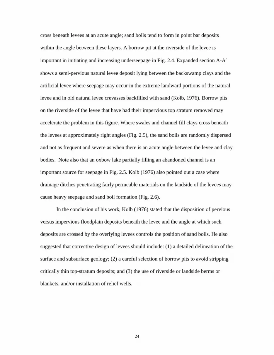
boils reported at those areas. Figure 2.4 shows how clay channel fillings and swales can
24
cross beneath levees at an acute angle; sand boils tend to form in point bar deposits
within the angle between these layers. A borrow pit at the riverside of the levee is
important in initiating and increasing underseepage in Fig. 2.4. Expanded section A-A′
shows a semi-pervious natural levee deposit lying between the backswamp clays and the
artificial levee where seepage may occur in the extreme landward portions of the natural
levee and in old natural levee crevasses backfilled with sand (Kolb, 1976). Borrow pits
on the riverside of the levee that have had their impervious top stratum removed may
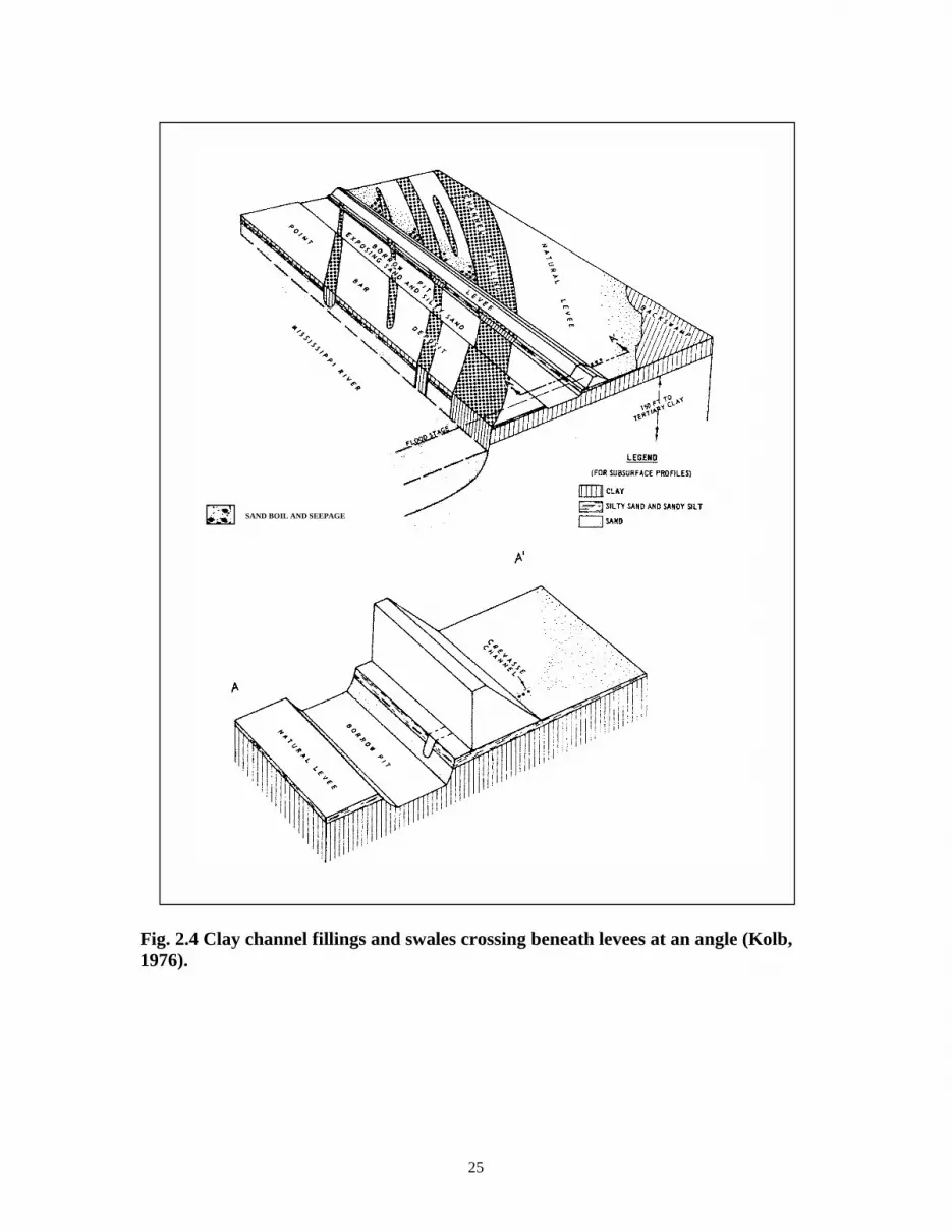
accelerate the problem in this figure. Where swales and channel fill clays cross beneath
the levees at approximately right angles (Fig. 2.5), the sand boils are randomly dispersed
and not as frequent and severe as when there is an acute angle between the levee and clay
bodies. Note also that an oxbow lake partially filling an abandoned channel is an
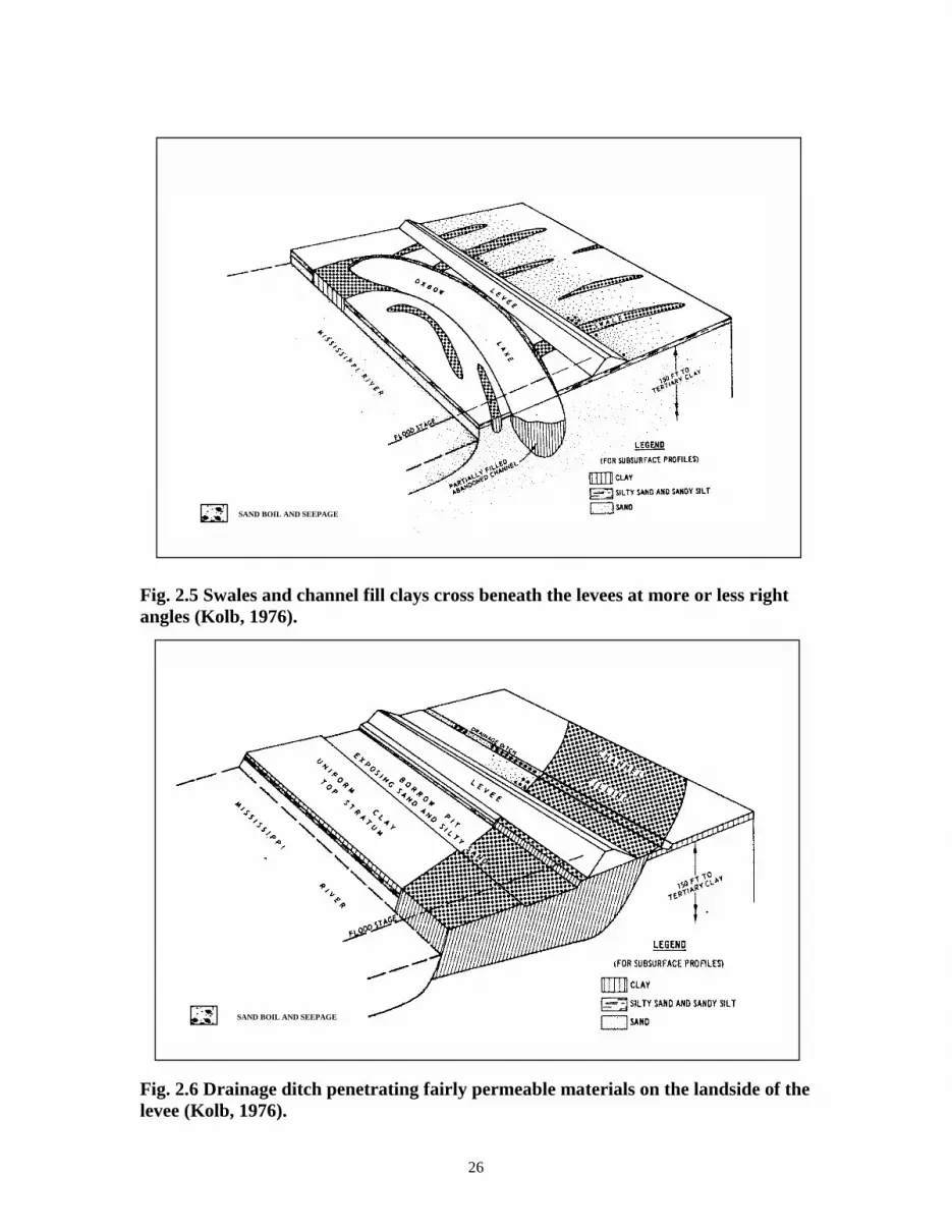
important source for seepage in Fig. 2.5. Kolb (1976) also pointed out a case where
drainage ditches penetrating fairly permeable materials on the landside of the levees may
cause heavy seepage and sand boil formation (Fig. 2.6).
In the conclusion of his work, Kolb (1976) stated that the disposition of pervious
versus impervious floodplain deposits beneath the levee and the angle at which such
deposits are crossed by the overlying levees controls the position of sand boils. He also
suggested that corrective design of levees should include: (1) a detailed delineation of the
surface and subsurface geology; (2) a careful selection of borrow pits to avoid stripping
critically thin top-stratum deposits; and (3) the use of riverside or landside berms or
blankets, and/or installation of relief wells.
25
Fig. 2.4 Clay channel fillings and swales crossing beneath levees at an angle (Kolb, 1976).
SAND BOIL AND SEEPAGE
26
Fig. 2.5 Swales and channel fill clays cross beneath the levees at more or less right angles (Kolb, 1976). Fig. 2.6 Drainage ditch penetrating fairly permeable materials on the landside of the levee (Kolb, 1976).
SAND BOIL AND SEEPAGE
SAND BOIL AND SEEPAGE
27
2.5 Previous Studies on Levee Underseepage Conducted by USACE
The first investigation of potential levee underseepage was initiated by the
USACE Mississippi River Commission in 1937 in response to problems caused by high
water conditions. More detailed study was carried out by the USACE Waterways
Experiment Station (WES), Vicksburg, MS in the 1940’s. Procedures to evaluate the
quantity of underseepage, uplift pressures and hydraulic gradients were developed based
on closed-form solutions for differential equations of seepage flow presented by Bennett
(1946). In 1956, a technical memorandum, TM 3-424 was published by the USACE
Waterways Experiment Station documenting the analysis of underseepage and design of
control measures for Lower Mississippi Valley levees (Mansur et al. 1956). In this
document, the top stratum landside of levees is classified into one of three categories: (1)
no top stratum; (2) top stratum of insufficient thickness to resist hydrostatic pressures that
can develop; and (3) top stratum of sufficient thickness to resist hydrostatic pressures that
can develop during the maximum design flood. Kolb (1976) discussed underseepage data
collected by USACE Vicksburg District along a randomly selected 40-mile reach of the
river during the 1973 flood. He pointed out the most dangerous top stratum category as
the second category listed by Mansur et al., 1956. In this category, artesian pressures can
build up beneath the top stratum landside of the levee to a range of 25% to 75% of the net
head on the levee, and may extend significant distances landward of a levee.
Mansur et al. (1956) classified seepage as heavy, medium and light. Turnbull and
Mansur (1961) presented seepage conditions and upward gradients through the top
stratum measured by piezometers during the 1950 high water (Table 2.1). During the
high water of 1950, sand boils were observed in a hydraulic gradient range of 0.5 to 0.8.
In developing these seepage conditions, sites were eliminated where the top stratum
28
thickness was less than 5 ft or greater than 15 ft (Technical Letter, ETL 1110-2-555,
1997).
Table 2.1 Seepage Conditions and Exit Gradients During the 1950 High Water (Turnbull and Mansur, 1961).
Seepage Condition Amount of Seepage (Q/H) Exit Gradient
Light to no seepage < 5 gal/min/100 ft of levee 0-0.5
Medium seepage 5 - 10 gal/min/100 ft of levee 0.2-0.6
Heavy seepage > 10 gal/min/100 ft of levee 0.4-0.7
Turnbull and Mansur (1961) summarized the design and analysis procedure of
levees presented in TM 3-424. Department of Army published in 1978 (and updated in
2000) an Engineer Manual (EM) 1110-2-1913 “Design and Construction of Levees”.
Other than advanced numerical modeling, this Engineer Manual represents the state-of-
practice analysis method for evaluating hydraulic gradient due to levee underseepage
(Gabr et al., 1996).
The Army Corps of Engineers investigated possible remedial measures to
underseepage problems, which are discussed below. The most common underseepage
control measures include pressure relief wells, landside seepage berms, riverside
blankets, drainage blankets or trenches, cutoffs, and sublevees. Muskat (1937) presented
a design methodology for relief wells. Middlebrooks and Jervis (1947) revised Muskat’s
method to include partial penetration of the relief wells. Barron (1948) presented a
design methodology for fully penetrating relief wells. The Department of the Army
published Engineer Manual (EM) 1110-2-1905 “Design of Finite Relief Well Systems”
in 1963 and EM 1110-2-1914 “Design, Construction, and Maintenance of Relief Wells”
in 1992. Mansur et al. (1956) stated that pressure relief wells, riverside blankets, and
29
landside seepage berms are generally applicable for Mississippi River levees. Sublevees
and drainage blankets or trenches are applicable in certain special situations.
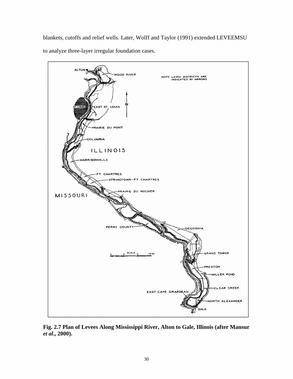
Wolff (1974) and the U.S. Army Engineer District, St. Louis (1976) studied the
performance of 200+ mile levee system along the middle Mississippi River from Alton to
Gale (Fig. 2.7).
It was reported that the use of the Corps method outlined in Engineer Manual
(EM) 1110-2-1913 resulted in a reliable design of levees. It was also concluded that the
existing procedure has deficiencies in characterization of a two layer subsurface profile
and the inability to model levee bends at corners. Cunny (1980) summarized piezometer
data for levees in the Rock Island District, Illinois. Cunny reported that the probability of
sand boil occurrence increases with geologic discontinuities. Daniel (1985) reviewed
Cunny’s report and the other Rock Island data and found that sand boils were observed at
gradients ranging from 0.54 to 1.02. A similar statement was also reported earlier in TM
3-424.
Wolff (1987) studied the application of numerical methods to levee underseepage
analysis and pointed out the advantages of special purpose computer programs over
traditional underseepage analysis and general-purpose numerical analysis programs.
Wolff (1989) developed the computer program LEVEEMSU for analysis of levee
underseepage. LEVEEMSU was also used to analyze actual data at a number of levee
reaches and back-calculate field permeability values. Cunny et al. (1989) also developed
a computer program, LEVSEEP, to perform regular underseepage analysis outlined in
EM 1110-2-1913, TM 3-424, EM 1110-2-1602, as well as to calculate reduced seepage
quantities with the choice of control measures including seepage berms, riverside
30
blankets, cutoffs and relief wells. Later, Wolff and Taylor (1991) extended LEVEEMSU
to analyze three-layer irregular foundation cases.
Fig. 2.7 Plan of Levees Along Mississippi River, Alton to Gale, Illinois (after Mansur et al., 2000).
31
2.5 Current Underseepage Analysis Methods
In general, approximate methods of solution to confined flow problems include
models such as Hele-Shaw models, relaxation methods (numerical analysis), and small-
scale laboratory models. Advanced numerical modeling and 2-D finite element analysis
programs provide sophisticated analysis of seepage flow. Boundary fitted coordinate
methods also show promise as a method of analyzing seepage flow problems (Thompson
et al. 1977; Thompson and Warsi, 1982; Thompson et al. 1985, and Hartono, 2002).
The transient effects in seepage have been studied under conditions of partial
saturation (EM 1110-2-1901, Seepage Analysis and Control for Dams). The flow in
partially or unsaturated soils is considered in a transient state. Therefore, transient effects
in seepage are normally studied as the migration of a wetting front into unsaturated soils
and variations in hydraulic conductivity according to soil water retention curves. Viscous
flow models have been used to study transient flow (EM 1110-2-1901). A viscous flow
model was constructed at USACE Waterways Experiment Station (WES) to simulate
seepage conditions induced in streambanks by sudden drawdowns of the river level. The
results from the model study were compared with field observations, finite difference,
and finite element methods (Desai 1970, Desai 1973). Two and three-dimensional finite
element seepage computer programs for confined and unconfined flow problems were
developed at WES. Steady-state and transient problems can be solved with these
computer programs (Tracy 1973a, Tracy 1973b). Transient problems can be treated as a
series of steady-state problems. The studies lead by USACE formed a basis for further
development of commonly used finite element seepage programs. GMS/SEEP2D is a 2D
finite element model that can be used to model steady-state confined, partially confined
32
and unconfined flow. Another finite element seepage analysis program, SEEP/W
performs transient seepage analysis considering hydraulic conductivity and water content
changes as a function of pore water pressure. Complex geometries, non-homogenous, and
anisotropic soil features can be modeled by these finite element models.
For seepage analysis under levees, U.S. Army Corps of Engineers, Design
Guidance on Levees, EM 1110-2-1913, recommends use of numerical analysis models
such as LEVSEEP and LEVEEMSU or finite element methods such as CSEEP which
include two-layer or three-layer subsurface characterization (ETL 1110-2-555, 1997).
The computer program LEVSEEP is based on the modeling of the steady-state flow
domain with Bennett’s (1946) analytical solutions for underseepage and the method of
fragments for cutoff analyses. LEVSEEP provides similar analysis with the hand methods
of analysis outlined in EM 1110-2-1913, EM 1110-2-1602, and TM 3-424 (Brizendine et
al. 1995). LEVEEMSU is based on one-dimensional simplification of the steady-state
flow domain using the finite difference method. LEVEEMSU solves Bennett’s (1946)
differential equation for irregular foundation geometry and non-uniform soil properties.
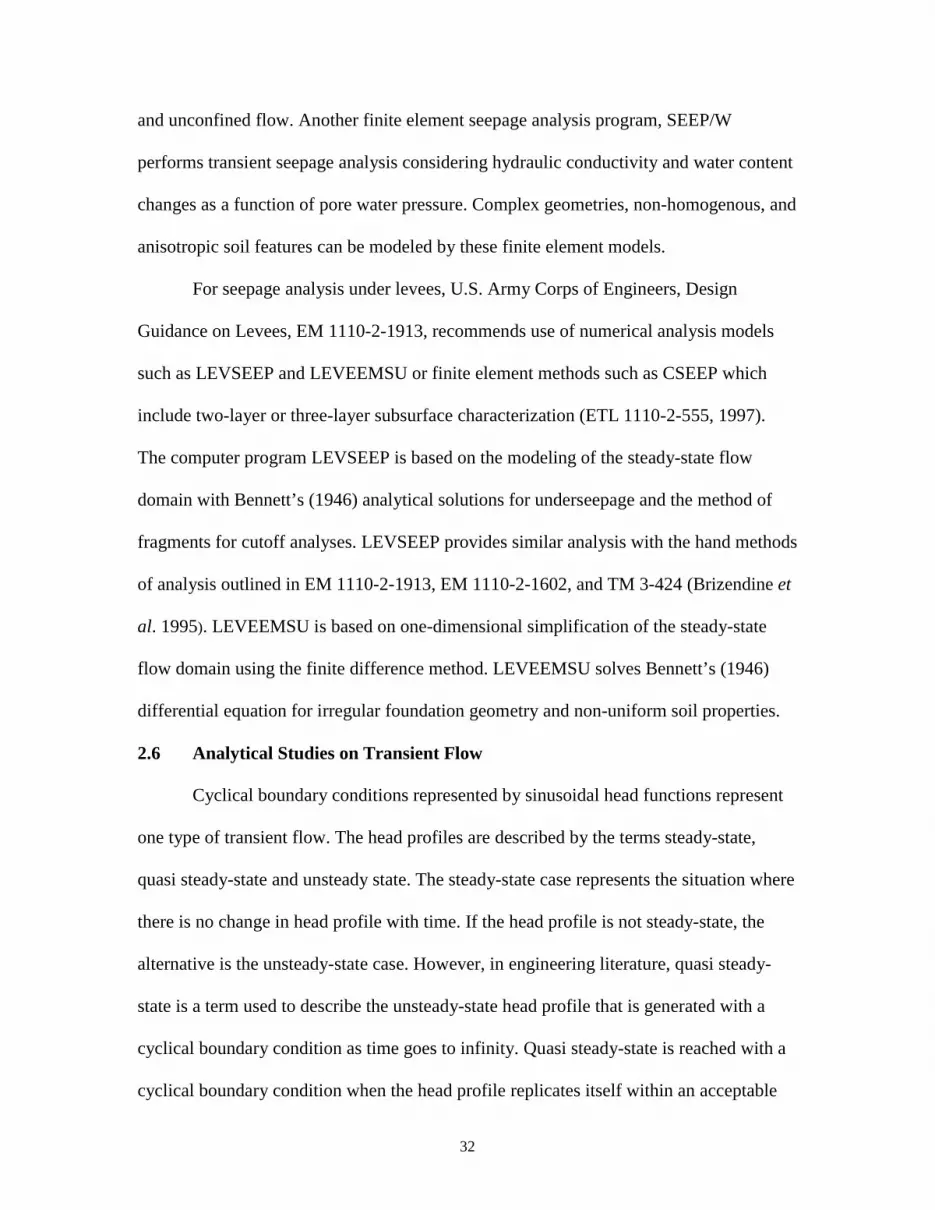
2.6 Analytical Studies on Transient Flow
Cyclical boundary conditions represented by sinusoidal head functions represent
one type of transient flow. The head profiles are described by the terms steady-state,
quasi steady-state and unsteady state. The steady-state case represents the situation where
there is no change in head profile with time. If the head profile is not steady-state, the
alternative is the unsteady-state case. However, in engineering literature, quasi steady-
state is a term used to describe the unsteady-state head profile that is generated with a
cyclical boundary condition as time goes to infinity. Quasi steady-state is reached with a
cyclical boundary condition when the head profile replicates itself within an acceptable
33
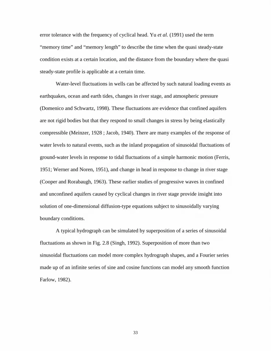
error tolerance with the frequency of cyclical head. Yu et al. (1991) used the term
“memory time” and “memory length” to describe the time when the quasi steady-state
condition exists at a certain location, and the distance from the boundary where the quasi
steady-state profile is applicable at a certain time.
Water-level fluctuations in wells can be affected by such natural loading events as
earthquakes, ocean and earth tides, changes in river stage, and atmospheric pressure
(Domenico and Schwartz, 1998). These fluctuations are evidence that confined aquifers
are not rigid bodies but that they respond to small changes in stress by being elastically
compressible (Meinzer, 1928 ; Jacob, 1940). There are many examples of the response of
water levels to natural events, such as the inland propagation of sinusoidal fluctuations of
ground-water levels in response to tidal fluctuations of a simple harmonic motion (Ferris,
1951; Werner and Noren, 1951), and change in head in response to change in river stage
(Cooper and Rorabaugh, 1963). These earlier studies of progressive waves in confined
and unconfined aquifers caused by cyclical changes in river stage provide insight into
solution of one-dimensional diffusion-type equations subject to sinusoidally varying
boundary conditions.
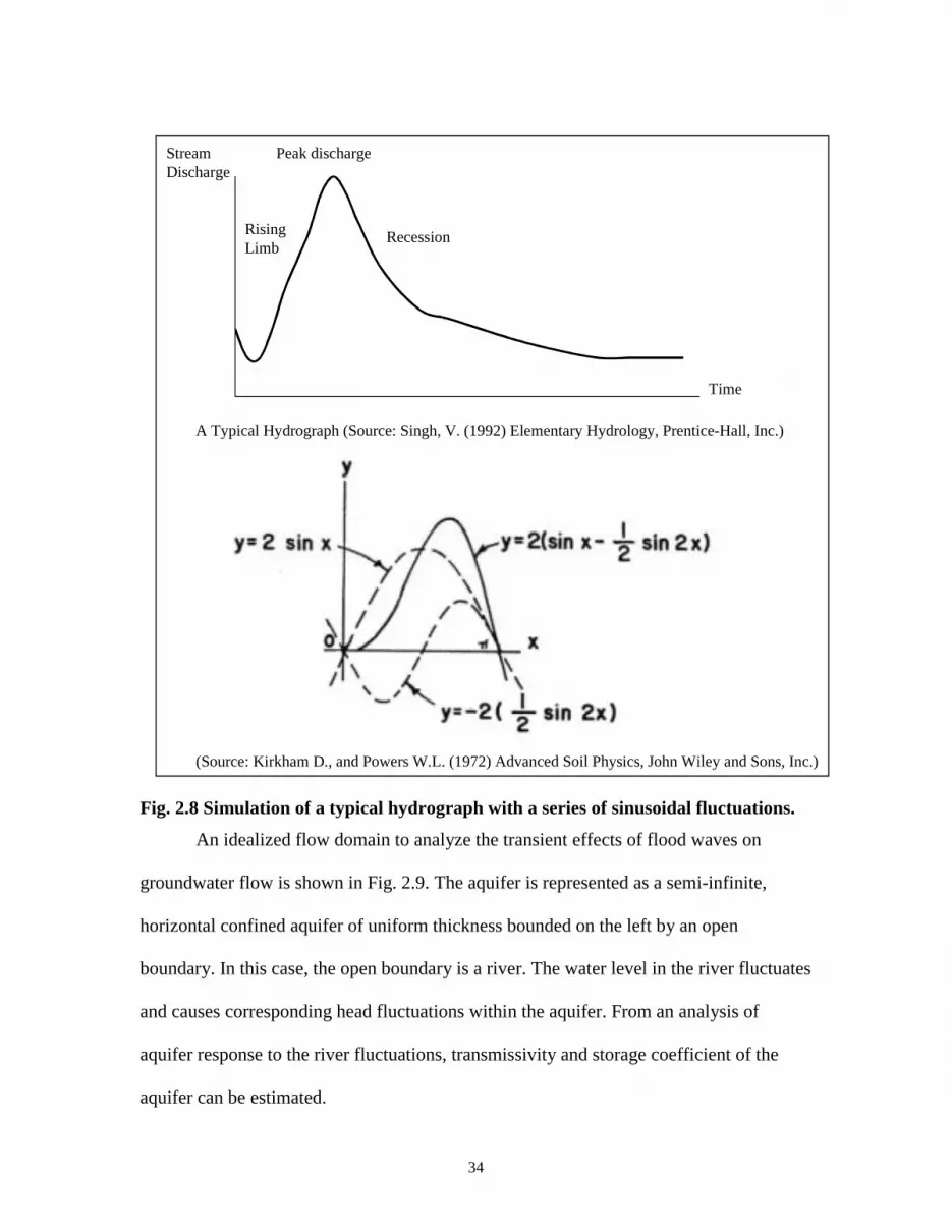
A typical hydrograph can be simulated by superposition of a series of sinusoidal
fluctuations as shown in Fig. 2.8 (Singh, 1992). Superposition of more than two
sinusoidal fluctuations can model more complex hydrograph shapes, and a Fourier series
made up of an infinite series of sine and cosine functions can model any smooth function
Farlow, 1982).
34
Fig. 2.8 Simulation of a typical hydrograph with a series of sinusoidal fluctuations.
An idealized flow domain to analyze the transient effects of flood waves on
groundwater flow is shown in Fig. 2.9. The aquifer is represented as a semi-infinite,
horizontal confined aquifer of uniform thickness bounded on the left by an open
boundary. In this case, the open boundary is a river. The water level in the river fluctuates
and causes corresponding head fluctuations within the aquifer. From an analysis of
aquifer response to the river fluctuations, transmissivity and storage coefficient of the
aquifer can be estimated.
StreamDischarge
Time
RisingLimb
Recession
Peak discharge
A Typical Hydrograph (Source: Singh, V. (1992) Elementary Hydrology, Prentice-Hall, Inc.)
(Source: Kirkham D., and Powers W.L. (1972) Advanced Soil Physics, John Wiley and Sons, Inc.)
35
Fig. 2.9 Representation of simplified one-dimensional flow as a function of surface-water stage (source: USACE, EM 1110-2-1421).
One-dimensional flow is described in many textbooks by the equation for linear,
non-steady flow in a confined aquifer:
2
2
xh
ST
th
∂∂=
∂∂ (2.8)
where h is the rise or fall of hydraulic head in the aquifer, x is the distance from aquifer-
river intersection, t is time, T is aquifer transmissivity, and S is aquifer storage
coefficient. The solution of Equation 2.8 subject to a fluctuating boundary condition was
presented by Ferris 1951; Cooper and Rorabough 1963; Pinder et al. 1969; and Hall and
Moench 1972. Ferris (1951) observed that wells near bodies of tidal water often show
sinusoidal fluctuations of water level in response to periodic changes in water stage. He
presented a quasi steady-state solution to the problem. He also presented expressions to
determine aquifer diffusivity (T/S) based on the observed values of amplitude, lag,
velocity, and wavelength of the sinusoidal changes in groundwater level. If the time lag
between surface and groundwater maximum and minimum stages is known then aquifer
diffusivity can be estimated by using the following formula (Engineer Manual, EM 1110-
2-1421, Equation 6-9)
x
Maximum stage
Reservoir
h0
h(x,0)
Land surface
Piezometric surface h(x,t)
Aquifer
h
36
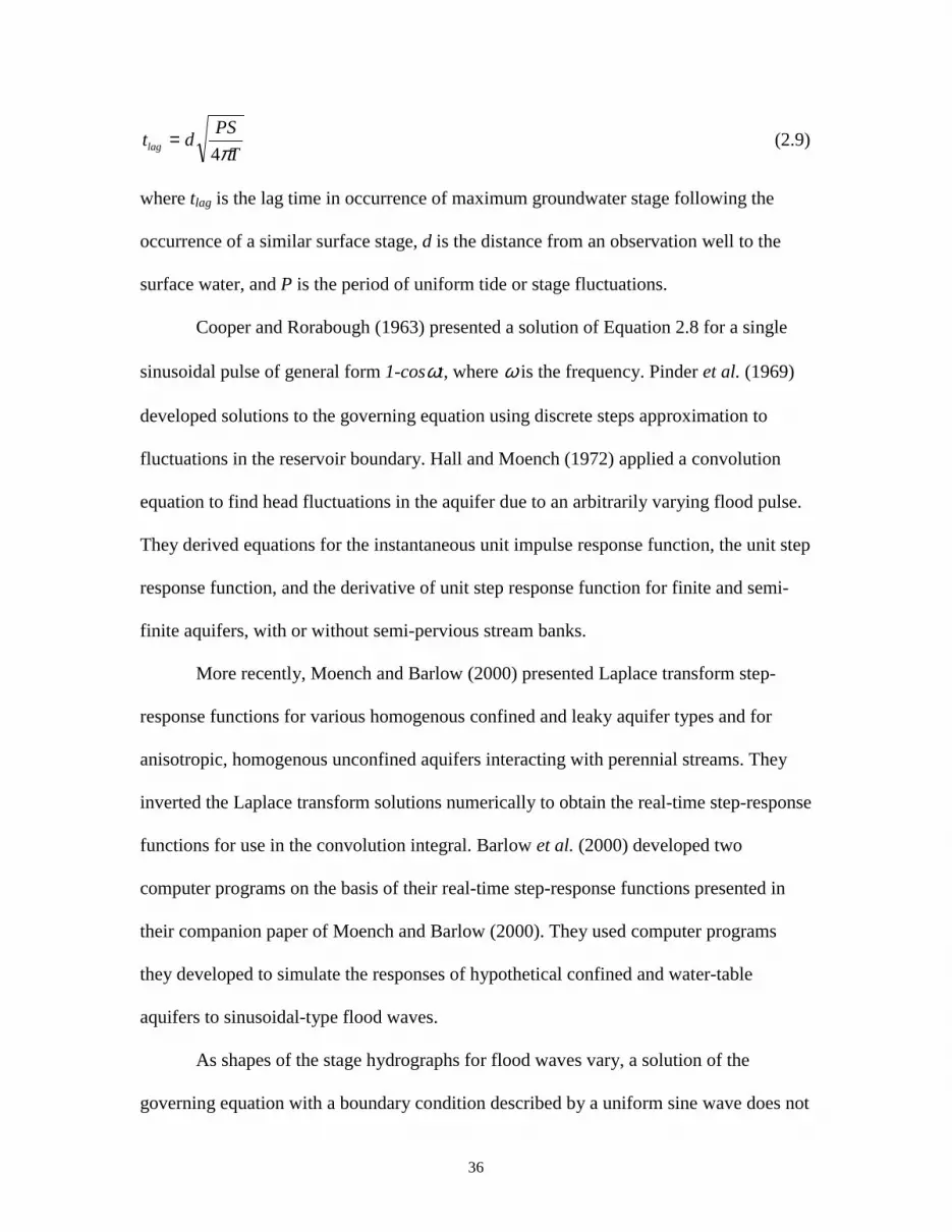
TPSdtlag π4
= (2.9)
where tlag is the lag time in occurrence of maximum groundwater stage following the
occurrence of a similar surface stage, d is the distance from an observation well to the
surface water, and P is the period of uniform tide or stage fluctuations.
Cooper and Rorabough (1963) presented a solution of Equation 2.8 for a single
sinusoidal pulse of general form 1-cosωt, where ω is the frequency. Pinder et al. (1969)
developed solutions to the governing equation using discrete steps approximation to
fluctuations in the reservoir boundary. Hall and Moench (1972) applied a convolution
equation to find head fluctuations in the aquifer due to an arbitrarily varying flood pulse.
They derived equations for the instantaneous unit impulse response function, the unit step
response function, and the derivative of unit step response function for finite and semi-
finite aquifers, with or without semi-pervious stream banks.
More recently, Moench and Barlow (2000) presented Laplace transform step-
response functions for various homogenous confined and leaky aquifer types and for
anisotropic, homogenous unconfined aquifers interacting with perennial streams. They
inverted the Laplace transform solutions numerically to obtain the real-time step-response
functions for use in the convolution integral. Barlow et al. (2000) developed two
computer programs on the basis of their real-time step-response functions presented in
their companion paper of Moench and Barlow (2000). They used computer programs
they developed to simulate the responses of hypothetical confined and water-table
aquifers to sinusoidal-type flood waves.
As shapes of the stage hydrographs for flood waves vary, a solution of the
governing equation with a boundary condition described by a uniform sine wave does not
37
describe the actual domain adequately (Engineer Manual, EM 1110-2-1421). The discrete
steps approach is not restricted to fluctuation of sinusoidal or uniform asymmetric curves
and allows the use of a stage hydrograph of any shape. An alternative approach for
representing the flood wave boundary has been shown in Figure 2.8.
Another application of cyclical boundary conditions in analytical solutions are the
studies on tracer transport models in soils and contaminant transport in rivers. Logan et
al. (1996) studied a one-dimensional model of transport of a chemical tracer in porous
media with periodic Dirichlet and periodic flux type boundary conditions. Alshawabkeh
and Adrian (1997) studied pollutant transport in a river subject to a sinusoidally varying
boundary condition. They applied complex variables and the Laplace transform method
to solve for the pollutant concentration distribution. Oppenheimer et al. (1999) proved
that an unsteady-state solution approaches to the quasi steady-state solution with time.
Adrian et al. (2001) developed a tracer transport model in a soil column with a periodic
loading function, which varies as a sinusoidal curve. They solved the governing equation
by applying superposition, Laplace transform and convolution integral, and introduced
complex variables to evaluate the convolution integral.
2.8 Cumulative Effects
Cumulative effects of seepage under levees can compromise levee safety. A
stratum of sands under seepage flow begins to heave at a particular value of seepage. This
heave is related to the size, velocity, and amount of particles that wash away (Peter,
1982). The deformation due to heave may be reversible; however, complete recovery of
this expansion is unlikely. When the same stratum of sands is exposed to a subsequent
flood, movement of fine particles is expected to be more severe than it was during a
previous flood. Besides when piping is localized at the landside levee toe, even if there is
38
no external evidence of a sand boil, there are few if any mechanisms which would bring
about healing of a pipe located immediately below a rigid, non-deforming levee. Peter
(1982) also noted another serious problem that can contribute to cumulative effects. As
the river level drops, the seepage water that had been on the landside may flow back from
its former discharging point toward the river leading to backward erosion which may
promote development of a pipe on the riverside of the levee. This erosion gradually
enlarges and shortens the seepage channel and may cause additional cumulative changes
leading to enlargement and lengthening of the internal pipe. Figure 2.10 shows the
mechanisms related to the cumulative effects in which backward erosion takes place.
Fig. 2.10 A schematic diagram of underseepage mechanisms that contribute to cumulative effects both during a flood and immediately after a flood. Although there is no reported study emphasizing the cumulative effects in
underseepage problems of levees, Turnbull and Mansur’s study in 1961 implies the
existence of cumulative effects. During the 1950 high water, upward gradients through
the top stratum at some control sites were measured by piezometers. The gradient
required to cause sand boils varied considerably at the different sites, possibly because at
flood stage
Top stratum
normal stage
sand boil
forward erosionduring flood
backward erosionafter flood
piping piping
ponded water Levee
39
sites where sand boils had developed previously only fairly low excess heads may have
been needed to reactivate these boils in 1950. At sites where no sand boils had occurred
in the past, higher gradients may have been required to initiate formation of the boils
(Turnbull and Mansur, 1961). They also suggested that pressure relief resulting from the
boil might have lowered piezometer readings in the area (Wolff, 2002). Currently,
USACE Engineer Research and Development Center (ERDC) in Vicksburg, MS is
working on research on cumulative effects of piping under levees as part of the
Innovative Flood Damage Research Program (IFDR) sponsored by USACE (Wolff,
2002).
2.9 Summary and Concluding Remarks
In the literature, seepage under levees associated with sand boils has been studied
in detail. Qualitative and quantitative models exist to describe the mechanisms of seepage
erosion. Geology of Lower Mississippi River Valley has also been well explored.
Engineers should consider the complex geology in design of levees and underseepage
analysis. As in all civil engineering problems, appropriate assumptions are required to
solve confined flow problems. Overall, a variety of tools, design manuals, specifications
and guidelines are successfully in use to perform a seepage analysis for levees. However,
the literature depicts that transient flow conditions associated with sand boil problems
have not been studied in detail in levee underseepage analysis.
As presented in Section 2.6, there are numerous analytical studies on transient
flow and a variety of solution methods to the general one-dimensional flow equation
(Equation 2.8) subject to fluctuating boundary conditions. However, there is relatively
little information on relating these transient flow models to critical hydraulic gradients
40
and sand boil formation. In addition, as noted before, there is almost no information on
the cumulative effects of seepage under levees and its relationship to piping.
Overall, the background and literature review presented in this chapter implies
that the objectives set in this dissertation are important research topics. Successful
completion of the research work would bring a new perspective to the problem.
2.10 List of Symbols and Acronyms
C = creep coefficient (dimensionless)
Cc = coefficient of curvature (dimensionless)
Cu = uniformity coefficient (dimensionless)
CW = weighted creep ratio (dimensionless)
d = distance (L)
d10 = grain diameter corresponding to 10% finer in grain size distribution curve (L)
d30 = grain diameter corresponding to 30% finer in grain size distribution curve (L)
d50 = grain diameter corresponding to 50% finer in grain size distribution curve (L)
d60 = grain diameter corresponding to 60% finer in grain size distribution curve (L)
e = void ratio of soil (dimensionless)
γsub = submerged unit weight of soil (WL-3)
γw = unit weight of water (WL-3)
Gs = specific gravity of soil (dimensionless)
h = hydraulic head (L)
h = total head loss (L)
hx = head beneath top stratum at distance x from landside toe of the levee (L)
ic = critical hydraulic gradient (dimensionless)
k0 = initial intrinsic permeability (L2)
41
L = length of seepage path (L)
Lh = distance along horizontal contacts (L)
LV = distance along vertical contacts (L)
n0 = initial porosity of soil (dimensionless)
P = period of uniform fluctuations (T)
S = aquifer storativity (dimensionless)
t = time (T)
tlag = time lag (T)
T = aquifer transmissivity (LT-2)
τc = critical tractive shear stress ( MT-2L-1)
x = horizontal coordinate (L)
zt = thickness of landside top stratum
EM = Engineer Manual
ERDC = Engineer Research and Development Center
ETL = Engineer Technical Letter
GMS = Groundwater Modeling System
IFDR = Innovative Flood Damage Research Program
USACE = United States Army Corps of Engineers
WES = Waterways Experiment Station
TM = Technical Manual
42
CHAPTER 3 TRANSIENT FLOW MODEL IN A CONFINED AQUIFER
3.1 Introduction
The objective of this chapter was to develop analytical models that describe the
hydraulic head in a confined aquifer on the landside of a levee system during the rising
limb of a flood wave. One-dimensional linear-laminar saturated flow conditions in a
homogenous, isotropic confined aquifer were studied. The top stratum is assumed as
impervious. The models used a sinusoidally varying boundary condition to simulate the
effects of the rising river stage. In these models, the governing equation is the diffusion
equation that was developed under Darcy’s law, and the law of conservation of mass
(Freeze and Cherry, 1979). Darcy’s law is valid as long as the Reynolds number based on
grain diameter does not exceed some value between 1 to 10 (Bear, 1972).
Two solutions were presented. Section 3.2 details the development of the transient
flow model by the Laplace transform method. Section 3.3 presents an approximate
solution to the same problem. The analyses were extended to falling limb of a flood wave
due to the fact that some field observations indicated critical situations during falling
river stages (Section 2.3.1).
3.2 Analytical Modeling of Transient Hydraulic Head in a Confined Aquifer by Laplace Transform Method
A schematic view of the model is shown in Fig. 3.1. The governing equation for a
one-dimensional model of transient seepage through a confined aquifer is known as the
diffusion equation (Freeze and Cherry, 1979)
21
21
xh
ST
th
∂∂
=∂∂
(3.1)
43
where h1 is the hydraulic head (L), T is the transmissivity (L2/T), t is time (T), S is the
storativity, which is dimensionless and x is the distance from the entrance to the confined
aquifer (L). The initial head at time t = 0 is 0, assuming mean low river level is well
below the origin which is the most common case. During high water, an initial head of H0
is developed. During the flood, fluctuation of this head is typical and defined as H1sin(ωt)
in the analysis. Another boundary condition is the head h = 0 when x approaches infinity,
which represents no influence of head far landward. Therefore, initial and boundary
conditions are selected as
( ) 00,1 =xh (3.2)
( ) ( )tHHth ωsin,0 101 += (3.3)
( ) 0,lim 1 →∞→
txhx
(3.4)
where H0 is the initial hydraulic head applied to the aquifer, H1 is the amplitude of the
variation from the initial hydraulic head and ω is the frequency of the flood wave. To
make the problem realistic Ho and H1 are positive or zero with the constraint that Ho ≥ H1.
Fig. 3.1 Schematic view of confined flow under a levee.
Flood stage
Top stratum
Pervious substratum
Top stratum
y
x
Levee
44
The approach in setting up the governing equations is similar to the approach
followed by Ozisik (1968) and Alshawabkeh and Adrian (1997). We define a new
problem with dependent variable h2(x, t) that is identical to Equations 3.1, 3.2, and 3.4
but the boundary condition is
( ) ( )tHHth ωcos,0 102 += (3.5)
Each term in the first problem is multiplied by the complex number i and is added
to the second problem. Then, a new complex variable is introduced
( ) ( ) ( )txihtxhtxh ,,, 12 += (3.6)
where h1(x,t), the imaginary part of solution, satisfies the original problem Equations 3.1
to 3.4, and h2(x,t), the real part of the solution, satisfies the original problem with the
boundary condition (Equation 3.3 changed to Equation 3.5).
The governing equation for the complex transient seepage becomes
2
2
xh
ST
th
∂∂=
∂∂ (3.7)
( ) 00, =xh (3.8)
( ) ( ) ( )tiHHith ωexp1,0 10 ++= (3.9)
( ) 0,lim →∞→
txhx
(3.10)
In Equation 3.9, Euler’s relationship was used
( ) ( ) ( )titti ωωω sincosexp += (3.11)
The Laplace transform is applied to Equations 3.7 to 3.10 yielding
02
2
=− HTpS
dxHd (3.12)
45
ωipHH
piH
−++= 1
01)0( (3.13)
0)(lim →∞→
xHx
(3.14)
where the term )(xH is the Laplace transform of h(x,t) and p is the parameter in the
transform. The solution to the Equation 3.12 subject to Equations 3.13 and 3.14 is
−
−
++=TpSx
ipHH
pixH exp1)( 1
0 ω (3.15)
The inverse Laplace transforms from Carslaw and Jaeger (1963) applicable to the
Equation 3.15 in their original notation are
=
−
−
taerfc
peL
pa
21 (3.16)
++
−=
−−
−− t
taerfcet
taerfcee
peL aat
pa
ωωω
ωωω
22211 (3.17)
When the inverse transform is applied to the Equation 3.15, the solution becomes
( ) ( )
+
+
−
−
+
+=
tiTtSxerfc
TiSx
tiTtSxerfc
TiSx
tiH
TtSxerfcHitxh
ωω
ωω
ω
2exp
2exp
)exp(21
21,
1
0
(3.18)
Equation 3.18 should be separated into its real and imaginary parts to be
applicable to practical problems. The treatment of the real and imaginary parts of the
complex function (Equation 3.18) is the same as the procedure of Fourier as cited by
Tikhonov and Samarskii (1963). Separation of the expression
46
+
+
−
−
=
tiTtSxerfc
TiSx
tiTtSxerfc
TiSx
tiHtxE
ωω
ωω
ω
2exp
2exp
)exp(21),( 1 (3.19)
from Equation 3.18 into its real and imaginary parts is discussed term by term. By
applying Equation 3.11
+
=
2sinsin
2sincos
2cosexpexp θθθω
TSri
TSrx
TSr
TiSx mmm (3.20)
where r=ω and θ=π⁄2.
Next, the complementary error function can be expanded as (Abramowitz and Stegun,
1965)
( )112
iIRerfctiTtSxerfc +=
− ω (3.21)
( )222
iIRerfctiTtSxerfc +=
+ ω (3.22)
where
2cos
21 θrt
TtSxR −= (3.23)
2cos
22 θrt
TtSxR += (3.24)
2sin1 θrtI −= (3.25)
2sin2 θrtI = (3.26)
where r and θ were defined in Equation 3.20.
47
To evaluate the complementary error function of a complex number, the following
approximation is used (Abramowitz and Stegun, 1965):
As ( )iIRerf +≈ −1610ε , negligible error is introduced into the calculations when using
Equation 3.27. Now Equation 3.12 can be separated into the portion applicable to the sine
boundary condition, Equation 3.3 and cosine boundary condition, Equation 3.5. The
solution applicable for the sine boundary condition is
( ) ( ){ }txhTtSxerfcHtxh ,Im
2, 01 +
= (3.33)
Equation 3.33 is the solution to the problem introduced in Equations 3.1 through 3.4
where Im{h(x,t)} is the imaginary part of h(x,t)
48
( )
( )
( )
( )
+
−
+
−+
−
−
−
+
−
+
−
+
−
−+
−−
−
=
)2,2(2
sinsin
2,2(12
sincos
2cosexp
)1,1(2
sinsin
1,1(12
sincos
2cosexp
)sin(21
2,2(12
sinsin
)2,2(2
sincos
2cosexp
1,1(12
sinsin
)1,1(2
sincos
2cosexp
)cos(21)},(Im{
1
11
IRGTSrx
IRFTSrx
TSrx
IRGTSrx
IRFTSrx
TSrx
tH
IRFTSrx
IRGTSrx
TSrx
IRFTSrx
IRGTSrx
TSrx
tHtxh
θ
θθ
θ
θθ
ω
θ
θθ
θ
θθ
ω
(3.34)
This solution is applicable to determine time-dependent hydraulic head
development beneath the levee as a response to the stage fluctuations observed in the
river.
Similarly, the solution to the problem with cosine boundary equations, Equations
3.1, 3.2, 3.4 and 3.6, is
( ) ( ){ }txhTtSxerfcHtxh ,Re
2, 02 +
= (3.35)
where Re{h(x,t)} is the real part of h(x,t)
49
( )
( )
( )
( )
−
+
−
+
−
−+
−
−
−
+
−
+
−+
−
−
−
=
2,2(12
sinsin
)2,2(2
sincos
2cosexp
1,1(12
sinsin
)1,1(2
sincos
2cosexp
)sin(21
)2,2(2
sinsin
2,2(12
sincos
2cosexp
)1,1(2
sinsin
1,1(12
sincos
2cosexp
)cos(21)},(Re{
1
12
IRFTSrx
IRGTSrx
TSrx
IRFTSrx
IRGTSrx
TSrx
tH
IRGTSrx
IRFTSrx
TSrx
IRGTSrx
IRFTSrx
TSrx
tHtxh
θ
θθ
θ
θθ
ω
θ
θθ
θ
θθ
ω
(3.36)
Although the solution can be evaluated by a mathematics software, it is a long and
complex solution. Therefore, an approximate solution method to the same problem was
studied and will be presented in the next section.
3.3 Analytical Modeling of Transient Hydraulic Head in a Confined Aquifer by an Approximate Method
Jiao and Tang (1999) presented an approximate solution to a problem of
groundwater response to tidal fluctuation in a leaky confined aquifer. This solution
follows their method for an approximate transient seepage model in a confined aquifer. A
schematic view of the model is shown in Fig. 3.2.
50
Fig. 3.2 A schematic view of confined flow under a levee for an approximate solution. The governing equation for confined flow with initial and boundary conditions are
2
2
xh
ST
th
∂∂=
∂∂ (3.37)
( ) 00, hxh = (3.38)
( ) ( )thhth ωsin,0 10 += (3.39)
( ) 0,lim htxhx
=∞→
(3.40)
Let H=h-h0, then the differential equation becomes as follows with initial and boundary
conditions:
2
2
xH
ST
tH
∂∂=
∂∂
(3.41)
( ) 00, =xH (3.42)
( ) ( )thtH ωsin,0 1= (3.43)
( ) 0,lim =∞→
txHx
(3.44)
Equation 3.43 is in the form of ( ) ( )tiehtH ωIm,0 1= , then the solution can be assumed as:
Flood stage
Top stratum
Pervious substratum
Top stratum
y
x
Levee
51
( ) ( )tixeehtxH ωλ1, = (3.45)
Substitute the solution in Equation 3.41,
TSiωλ =2 (3.46)
Let iqp +−=λ , then
TSp
2ω= (3.47)
pTSq
2ω−= (3.48)
( ) ( )]Im[, 1qxtipxeeHtxH +−= ω (3.49)
( ) ( )qxtehtxH px += − ωsin, 1 (3.50)
Back to the original problem
( )
−+= − x
pTStehhtxh px
2sin, 10
ωω (3.51)
So, an approximate solution was found to the problem defined in Equations 3.37
through 3.40. This is an approximate solution because the final solution was initially
assumed as shown in Equation 3.45. Also, the final solution, Equation 3.51, does not
satisfy the initial condition specified in Equation 3.38. Thus, Equation 3.51 is called a
quasi steady-state solution, which is applicable, when time is large enough that the initial
condition is forgotten.
3.4 Results and Discussion
A typical levee section defined by the Army Corps is selected for analysis purpose
(EM 1110-2-1913). The thickness of sandy alluvium under Mississippi River levees
varies from 25 m to 45 m. The thickness of low permeable top layer under Mississippi
52
River levees ranges from 1.5 m to 37.5 m. The hydraulic conductivity of sandy alluvium
ranges from 0.1 cm/sec to 0.2 cm/sec (Turnbull and Mansur, 1961). Typical storativity
values for confined aquifers are 5x10⁻³, 5x10⁻⁴, 5x10⁻⁵ (Freeze and Cherry, 1979). In the
1993 floods, the net river level elevation change of the middle Mississippi River levees
was recorded as 4.8 to 6.7 m (Mansur et al. 2000). A net head of 5 m and a fluctuation of
1.5 m were selected in the analysis. The typical levee section with selected aquifer
parameters and hydraulic head is shown in Fig. 3.3.
Fig. 3.3 A typical levee section with selected parameters (not in scale).
The flood duration was selected as 60 days. The net head starts at 5 m, rises to the
peak of 6.5 m at time=30 days, and falls back to 5 m at time=60 days. Head development
over a distance of 200 m was determined, which included 50 m at riverside, a 50 m levee
base, and 100 m on the landside of the levee. The analysis was restricted to 100-m
landside of the levee because, as noted in the literature review, Li et al.(1996) reported
that there was no significant evidence of surface seepage beyond 100 m from the levee
north of Cairo, Illinois after the 1993 high water. The exit gradient at the levee toe and
landside of the levee was also calculated by taking the difference between the heads
above and below the top stratum and dividing by the top stratum thickness. Calculations
Net head:
5±1.5 m
Top stratum
Pervious substratum:25 m Top stratum: 5 m
Levee bottomwidth: 50 m
S=5x10⁻³
K=0.1 cm/sec
Levee toe at 100 m
y
x
53
were performed by MathCad 2000 software. Figures 3.4, 3.5, 3.6 and 3.7 show the results
by the Laplace transform method. Figures 3.8, 3.9, 3.10 and 3.11 show the results by the
approximate method.
Fig. 3.4 Transient head development at t=1 day and 30 days by Laplace transform method.
Fig. 3.5 Transient head development at x=1 m and x=100 m, levee toe, by Laplace transform method.
0 15 30 45 60 75 90 105 1203
3.5
4
4.5
5
5.5
6
6.5
7
Time (days)
Hea
d (m
)
6.499
3.493
h 1 t,( )
h 100 t,( )
1201 t
0 50 100 150 2003.5
4
4.5
5
5.5
6
6.5
7
Distance (m)
Hea
d (m
)
7
3.5
h x 1,( )
h x 30,( )
2000 x
54
Fig. 3.6 Transient exit gradient at the levee toe and at 200-m landside of levee by Laplace transform method. Fig. 3.7 Transient exit gradient at t=1 day and t=30 days at landside of the levee by Laplace transform method.
100 120 140 160 180 2000.8
0.9
1
1.1
1.2
1.3
1.4
Distance from levee toe (m)
Hyd
raul
ic g
radi
ent
1.278
0.841
i x 1,( )
i x 30,( )
200100 x
0 15 30 45 60 75 90 105 1200.6
0.7
0.8
0.9
1
1.1
1.2
1.3
1.4
Time (days)
Hyd
raul
ic g
radi
ent
1.278
0.697
i leveetoe x t,( )
i 200m x t,( )
1201 t
55
Fig. 3.8 Transient head development at t=1 day and t=30 days by the approximate method.
Fig. 3.9 Transient head development at x=1 m and x=100 m, levee toe, by the approximate method.
0 15 30 45 60 75 90 105 1203
3.5
4
4.5
5
5.5
6
6.5
7
Time (days)
Hea
d (m
)
6.5
3.5
h 1 t,( )
h 100 t,( )
1200 t
0 15 30 45 60 75 90 105 1203.5
4
4.5
5
5.5
6
6.5
7
Distance (m)
Hea
d (m
)
7
3.5
h x 1,( )
h x 30,( )
1200 x
56
Fig. 3.10 Transient exit gradient at the levee toe and at 200-m landside of the levee by the approximate method.
Fig. 3.11 Transient exit gradient at t=1 day and t=30 days at landside of the levee by the approximate method.
100 120 140 160 180 2000.9
1
1.1
1.2
1.3
1.4
Distance from levee toe (m)
Hyd
raul
ic g
radi
ent 1.293
0.9
i x 1,( )
i x 30,( )
200100 x
0 15 30 45 60 75 90 105 1200.6
0.7
0.8
0.9
1
1.1
1.2
1.3
1.4
Time (days)
Hyd
raul
ic g
radi
ent
1.293
0.707
i leveetoe 100 t,( )
i 200m 200 t,( )
1200 t
57
In general, both solutions give the expected 1.5 m sinusoidal head fluctuation with
an initial head of 5 m, with a peak at 30 days, and the part of the graphs after 30 days
represents the falling river stage (Figures 3.5 and 3.9). The approximate method performs
well compared with Laplace transform solution. Both solutions give minor head
dissipation with distance. Hydraulic head dissipates more rapidly at 100 m farther from
the levee toe by Laplace transform solution than by the approximate solution. Both
solutions assume a horizontal flow in semi-infinite layer. This assumption may be the
reason for minor head dissipations with distance. Table 1.1 shows the summary of the
results.
Table 3.1 Summary of the results by Laplace transform method and the approximate solution.
Head (m) and Hydraulic
gradient
Time (day) Laplace transform
Method
Approximate
Method
1 4.64 5.04 Head at levee toe (m)
30 6.39 6.46
1 4.20 5.00 Head at 100 m farther than
levee toe (m) 30 6.28 6.43
1 0.93 1.01 Hydraulic gradient at
levee toe 30 1.28 1.30
1 0.84 1.00 Hydraulic gradient at 100
m farther than levee toe 30 1.26 1.29
Time Lag in Head Development
One interesting common behavior is that both solutions show only a minor time
lag between the peak points of sinusoidal head curves with distance. In other words, the
peaks of head wave by Laplace transform solution (Fig. 3.5) and by the approximate
58
solution (Fig. 3.9) correspond to about 30 days at the levee toe and also at 100 m farther
than the levee toe. Based on Meehan’s observations of levee failure on the Feather River,
California, during the falling river stage in 1986 (reported in Chapter 2), one would
expect to observe a time lag between the peak points of the head waves at varying
distances. Figures 3.12 and 3.13 explore more on this subject.
Fig. 3.12 Transient head development beneath the levee at various distances from the river by Laplace transform method.
The time of occurrence of the peak points of the river hydrograph and the peak
hydraulic head of each head wave at various distances by Laplace transform and the
approximate method are also summarized in Table 3.2.
Both solution methods show a minor time difference between the peak heads at
various distances. As presented in Chapter 2, Ferris (1951) developed analytical
expressions to determine the aquifer diffusivity (T/S) based on the observed values of
amplitude, lag, velocity, and wavelength of the sinusoidal changes in groundwater level.
0 15 30 45 60 75 90 105 1203
3.5
4
4.5
5
5.5
6
6.5
7
Time (days)
Hea
d (m
)
6.499
3.476
h 1 t,( )
h 100 t,( )
h 200 t,( )
h 300 t,( )
1201 t
59
Fig. 3.13 Transient head development beneath the levee at various distances from the river by the approximate method. Table 3.2 Time of occurrence of the peak points of head wave at variable distances.
Methods Time and Head
at peak
x=1 m x=100m
(levee toe)
x=200 m x=300 m
Time (days) 30 31 31 32 Laplace Transform
Method Head (m) 6.50 6.39 6.28 6.18
Time (days) 30 30 31 31 Approximate
Method Head (m) 6.50 6.46 6.43 6.39
If the time lag between surface and groundwater maximum and minimum stages
is known, then the aquifer diffusivity can be estimated by using the following formula
(EM 1110-2-1421, Equation 6-9):
TPSdtlag π4
= (3.52)
where tlag is the lag time in the occurrence of the maximum groundwater stage following
the occurrence of a similar surface stage, d is the distance from an observation well to the
0 15 30 45 60 75 90 105 1203
3.5
4
4.5
5
5.5
6
6.5
7
Time (days)
Hea
d (m
)
6.5
3.5
h 1 t,( )
h 100 t,( )
h 200 t,( )
h 300 t,( )
1200 t
60
surface water, and P is the period of uniform tide or stage fluctuations. Equation 3.52 can
be applied to time lag analysis of transient head development due to river fluctuations. If
the same parameters as in the time lag analysis (d = 100 m, P = 60 days, S = 0.005,
T = 2160 m2/day) of Laplace transform and approximate methods were applied to
Equation 3.52, the time lag would result in 0.33 days for every 100-m of distance.
Only field studies can confirm the reliability of time lags estimated by the
transient flow models. As noted in the literature review, a levee collapse near Marysville,
California, occurred one day after the peak of the flood stage of Feather River. Part of the
time delay may have been due to the time required for sand boils to erode channels or
pipes under the levee, undermine it, and accelerate its failure. At Louisiana State
University Dairy Farm, however, an existing sand boil was reported to have responded
very quickly with the river stage fluctuations.
Base on limited field studies and an analytical estimation, the time lag results
presented in Table 1.2 appear to be reasonable.
3.5 Summary
Two transient flow models were developed to describe the hydraulic head
development beneath the landside levee in response to head fluctuations in the river. The
rising river stage was defined by a sinusoidally varying boundary condition. Both models
consider one-dimensional saturated flow conditions in a homogenous isotropic confined
aquifer. The first transient flow model was developed by solving the governing diffusion
equation and the boundary conditions (Equation 3.1 through 3.4) by Laplace transform
method. This solution method is complicated and can be evaluated only by a
61
mathematical software. Therefore, an approximate solution was also presented. The
results were evaluated for a typical levee section.
Both solutions result in expected head fluctuations. The approximate solution
performs well compared with the Laplace transform method. Both solutions give minor
head dissipation with time and distance. Both solutions also result in minor time lag
between the peak points of head waves at various distances. The distinctions between the
two solutions would become more apparent if the period of the river hydrograph
decreased, and if the development of heads and gradients at small times was sought. Then
the Laplace transform solution’s performance would be enhanced over the performance
of the approximate method.
The main objective of this chapter was to develop transient flow models by the
Laplace transform method and by an approximate method. This objective was satisfied.
The applicability and performance analysis of these flow models will be studied in the
following chapters.
3.6 List of Symbols
a = constant in inverse Laplace transform
d = distance (L)
E(x, t) = an expression for a part of the hydraulic head function
fn = function used to calculate error function
F = real function used to calculate an error function
gn = function used to calculate error function
ε = error of approximation
G = imaginary function used to calculate an error function
62
h = hydraulic head (L)
h(x, t) = hydraulic head function
h1(x, t) = imaginary part of hydraulic head function
h2(x, t) = real part of hydraulic head function
h0 = initial hydraulic head (L)
H0 = initial hydraulic head (L)
h1 = amplitude of the variation from the initial hydraulic head (L)
H1 = amplitude of the variation from the initial hydraulic head (L)
),( txH = Laplace transform of h(x, t)
i = imaginary unit where i2 = -1
I1, I2 = imaginary part of a complex variable
n = index of summation
λ = a complex variable
p = real part of the complex variable λ
p = complex number in Laplace transform
P = period of uniform stage fluctuations (T)
r = inverse of length squared (L-2)
q = imaginary part of the complex variable λ
R1, R2 = real part of a complex variable
S = aquifer storativity (dimensionless)
t = time (T)
tlag = time lag (T)
T = aquifer transmissivity (LT-2), also time dimension
63
x = horizontal coordinate (L)
y = variable in error function
zt = thickness of landside top stratum (L)
θ = phase angle for frequency ratio
ω = frequency of the flood wave (T-1)
64
CHAPTER 4 TRANSIENT FLOW MODEL WITH LEAKAGE OUT OF A CONFINED AQUIFER 4.1 Introduction
The objective of this chapter was to modify the analytical flow models developed in the
previous chapter by considering leakage occurring out of the confined aquifer. This
condition simulates the occurrence of loss of water by upward seepage and discharge
through sand boils at the landside of a levee or a flood wall system. The sand boils
develop at random points landside of the levee. The solution methods presented here
describe a homogenous leakage out of a confined aquifer through the landside of a levee
or a flood wall. The system considered is a subsurface confined aquifer with one-
dimensional saturated flow and semi-permeable layer on top. The aquifer is assumed to
be homogenous and isotropic. The models used a sinusoidally varying boundary
condition to simulate the effects of the rising river stage. In these models, the governing
equation is the diffusion equation that was developed under Darcy�s law, and the law of
conservation of mass. Two solutions were presented. The first solution used Laplace
transform method and followed the same methodology outlined in Section 3.2. The
second solution is an approximate solution and the same methodology outlined in Section
3.3 was followed. The analyses were extended to the falling limb of a flood wave due to
the fact that some field observations indicated critical situations during the falling river
stages (Section 2.3.1).
4.2 Analytical Modeling of Transient Hydraulic Head with Leakage Out of a Confined Aquifer by Laplace Transform Method The model was set up considering a subsurface system with a leaky confined
aquifer, and a semi-permeable layer on top representing the blanket layer (Fig. 4.1).
65
Fig. 4.1 Schematic view of confined flow under a flood wall with leakage out of an aquifer.
The initial head at time t = 0 is 0; assuming mean low river level is well below the
origin which is the most common case. During high water, an initial head of h0 is
developed. The fluctuation of this head is typical and defined as h1sin(ωt) in the analysis.
Another boundary condition is the head h = 0 when x approaches infinity which
represents a condition in which there is no influence of head far landward. Under these
conditions, the governing equation is:
hSL
xh
ST
th −
∂∂=
∂∂
2
2
(4.1)
where h is the hydraulic head, T is the transmissivity, t is time, S is the storativity, L is the
leakage, and x is the distance from the entrance to the confined aquifer. The initial and
boundary conditions may be given as
( ) 00, =xh (4.2)
( ) ( )thhth ωsin,0 10 += (4.3)
( ) 0,lim →∞→
txhx
(4.4)
Flood stage
Pervious substratum
y
x
Flood wall
Leakage
Top stratum
66
where h0 is the initial hydraulic head applied to the aquifer, h1 is the amplitude of the
variation from the initial hydraulic head and ω is the frequency of the flood wave,
ω = 2π/P, where P is the fluctuation period. To make the problem realistic h0 and h1 are
positive or zero with the constraint that h0 ≥ h1. The leakage, L is the ratio of hydraulic
conductivity of the semi-confining layer to the thickness of semi-confining layer. We
apply the transform h(x, t) = Y(x, t) exp (-L t/S) to Equations 4.1 to 4.4 get a homogenous
differential equation. The new set of equations becomes
2
2
xY
ST
tY
∂∂=
∂∂ (4.5)
0)0,( =xY (4.6)
( )
+
= t
SLtht
SLhtY expsinexp),0( 10 ω (4.7)
0),(lim =∞→
txYx
(4.8)
Now an approach similar to one followed by Ozisik (1968), and Alshawabkeh and
Adrian (1997) and outlined in Section 3.2 is followed. A new problem is defined with
dependent variable Z(x,t) that is identical to Equations 4.5, 4.6, and 4.8 but the boundary
condition is
( )
+
= t
SLtht
SLhtZ expcosexp),0( 10 ω (9)
Each term in the first problem is multiplied by the complex number i where 1−=i , and
the two problems are superimposed. Then, a new complex variable is introduced
( ) ( ) ( )txiYtxZtxH ,,,~ += (10)
67
where Y(x,t), the imaginary part of solution, satisfies the original problem Equations 4.5-
4.8, and Z(x,t) the real part of the solution, satisfies the original problem with the
boundary condition Equation 4.7 changed to Equation 4.9. The governing equation for
the complex transient seepage becomes
2
2 ~~
xH
ST
tH
∂∂=
∂∂ (4.11)
( ) 00,~ =xH (4.12)
( ) ( )
+
+= t
SLtiht
SLhitH expexpexp1),0(~
10 ω (4.13)
( ) 0,~lim →∞→
txHx
(4.14)
In Equation 4.13, Euler�s relationship was used
( ) ( ) ( )titti ωωω sincosexp += (4.15)
The Laplace transform is applied to Equations 4.11 to 4.14 yielding
02
2
=− HTpS
dxHd (4.16)
ωiSLp
hh
SLp
iH−−
+−
+= 10
1)0( (4.17)
0)(lim →∞→
xHx
(4.18)
where the term )(xH is the Laplace transform of ( )txH ,~ and p is the parameter in the
transform. The solution to Equation 4.16 subject to Equations 4.17 and 4.18 is
−
+−
+−
+=TpSx
SLip
hh
SLp
ixH exp1)( 10
ω (4.19)
68
The inverse Laplace transform from Carslaw and Jaeger (1963) applicable to Equation
4.19 in its original notation is
++
−=
−−
−− t
taerfcet
taerfcee
peL aat
pa
ωωω
ωωω
22211 (4.20)
When the inverse transform is applied to the Equation 4.19, the result is
( )
++
+
+
+−
+−
+
+
+
+
−
−
+=
tSLi
TtSxerfc
SLi
TSx
tSLi
TtSxerfc
SLi
TSx
tSLih
tSL
TtSxerfc
TLx
tSL
TtSxerfc
TLx
tSLhitxH
ωω
ωω
ω
2exp
2exp
exp21
2exp
2exp
exp2
1,~
1
0
(4.21)
Equation 4.21 should be separated into its real and imaginary parts to be
applicable to practical problems. The treatment of the real and imaginary parts of the
complex function (Equation 4.21) is the same as the procedure of Fourier as cited by
Tikhonov and Samarskii (1963) and detailed in Section 3.2. The same method is followed
here. Separation of the expression
++
+
+
+−
+−
=
tSLi
TtSxerfc
TL
TiSx
tSLi
TtSxerfc
TL
TiSx
tSLtihtxE
ωω
ωω
ω
2exp
2exp
exp)exp(21),( 1 (4.22)
from Equation 21 into its real and imaginary parts is discussed term by term. By applying
Euler�s relationship
69
+
=
+
2sinsin
2sincos
2cosexpexp θθθω
TSri
TSrx
TSr
TL
TiSx mmm (4.23)
where ( )
TLS
r22 +
=ω
and
=
LSωθ arctan .
Next, the complementary error function can be expanded as (Abramowitz and Stegun,
1965)
( )112
iIRerfctSLi
TtSxerfc +=
+− ω (4.24)
( )222
iIRerfctSLi
TtSxerfc +=
++ ω (4.25)
where
2cos
21 1
θtrTtSxR −= (4.26)
2cos
22 1
θtrTtSxR += (4.27)
2sin1 1
θtrI −= (4.28)
2sin2 1
θtrI = (4.29)
where S
LSr
22
1)( +
=ω
and θ are defined as in Equation 4.23.
To evaluate the complementary error function of a complex number, the
following approximation is used (Abramowitz and Stegun, 1965):
As ( )iIRerf +≈ −1610ε , and ( )iIRerf + has a maximum value of 2, negligible error is
introduced into the calculations when using Equation 4.30.
Now Equation 4.21can be separated into the portion applicable to the sine
boundary condition, Equation 4.3 and cosine boundary condition, Equation 4.5. The
solution to the original problem with sine boundary condition, Equations 4.1 through 4.4:
( ) ( ){ }
−= t
SLtxHtxh exp,~Im, (4.36)
where ( ){ }txH ,~Im is the imaginary part of ( )txH ,~ where
71
( )
( )
( )
( )
−
+
−+
−
−
−
+
−
+
−
+
−
−+
−−
−
+
+
+
−
−
=
)2,2(2
sinsin
2,2(12
sincos
2cosexp
)1,1(2
sinsin
1,1(12
sincos
2cosexp
exp)sin(21
2,2(12
sinsin
)2,2(2
sincos
2cosexp
1,1(12
sinsin
)1,1(2
sincos
2cosexp
exp)cos(21
2exp
2exp
exp21)},(~Im{
1
1
0
IRGrx
IRFrxrx
IRGrx
IRFrxrx
tSLth
IRFrx
IRGrxrx
IRFrx
IRGrxrx
tSLth
tSL
TtSxerfc
TLx
tSL
TtSxerfc
TLx
tSLhtxH
θ
θθ
θ
θθ
ω
θ
θθ
θ
θθ
ω
(4.37)
Similarly, the solution to the problem with cosine boundary condition, Equations 4.5, 4.6,
4.8, and 4.9 is
( ) ( ){ }
−= t
SLtxHtxZ exp,~Re, (4.38)
where ( ){ }txH ,~Re is the real part of ( )txH ,~ .
72
( )
( )
( )
( )
−
−
+
−
−−
−
−
+
+
−
+
−+
−
−
−
+
+
−
−
=
2,2(12
sinsin
)2,2(2
sincos
2cosexp
1,1(12
sinsin
)1,1(2
sincos
2cosexp
exp)sin(21
)2,2(2
sinsin
2,2(12
sincos
2cosexp
)1,1(2
sinsin
1,1(12
sincos
2cosexp
exp)cos(21
2exp
2exp
exp21)},(~Re{
1
1
0
IRFrx
IRGrxrx
IRFrx
IRGrxrx
tSLth
IRGrx
IRFrxrx
IRGrx
IRFrxrx
tSLth
tSL
TtSxerfc
TLx
tSL
TtSxerfc
TLx
tSLhtxH
θ
θθ
θ
θθ
ω
θ
θθ
θ
θθ
ω
(4.39)
Equation 4.39 is the solution to the problem introduced in Equations 4.1 through
4.4. This solution is applicable to determine time-dependent hydraulic head development
beneath the levee when there is leakage out of the aquifer in response to the stage
fluctuations observed in the river. Although the solution can be evaluated by
mathematical software, it is a long and complex solution. Therefore, an approximate
method to solve the same problem was studied and presented in the next section.
73
4.3 Analytical Modeling of Transient Hydraulic Head with Leakage Out of a Confined Aquifer by an Approximate Method
This solution follows the methodology outlined in Section 3.3 and originally
presented by Jiao and Tang (1999) for an approximate solution to a problem of
groundwater response to tidal fluctuation in a leaky confined aquifer. A schematic view
of the model is shown in Fig. 4.2.
Fig. 4.2 Schematic view of confined flow with leakage out of aquifer for an approximate solution.
The governing equations for confined flow with initial and boundary conditions
are
( )hhSL
xh
ST
th −−
∂∂=
∂∂
02
2
(4.40)
( ) 00, hxh = (4.41)
( ) ( )thhth ωsin,0 10 += (4.42)
( ) 0,lim htxhx
=∞→
(4.43)
where h0 is the initial head at t = 0, L is leakage, the ratio of hydraulic conductivity of the
semi-confining layer to the thickness of semi-confining layer with units time-1. Let
Flood stage
Pervious substratum
y
x
Flood wall
Leakage
Top stratum
74
H = h-h0, then the differential equation with initial and boundary conditions becomes:
HSL
xH
ST
tH +
∂∂=
∂∂
2
2
(4.44)
( ) 00, =xH (4.45)
( ) ( )thtH ωsin,0 1= (4.46)
( ) 0,lim =∞→
txHx
(4.47)
Equation 4.40 is in the form of ( ) ( )tiehtH ωIm,0 1= , the solution can be assumed as
( ) ( )tixeehtxH ωλ1, = (4.48)
The assumed solution (Equation 4.48) is substituted in Equation 4.44, and λ2 is derived
TL
TSi −= ωλ2 (4.49)
where λ must be a complex number. Let iqp +−=λ , then the real and imaginary parts
of Equation 4.49 are equated and p and q are derived as
2/12/122
21
−
+
=
TL
TS
TLp ω (4.50)
pTSq
2ω−= (4.51)
Substituting λ in Equation 4.48, and using the fluctuating boundary condition, Equation
4.46
( ) ( ) ]Im[, 1qxtipxeehtxH +−= ω (4.52)
( ) ( )qxtehtxH px += − ωsin, 1 (4.53)
Back to the original problem, the solution of Equation 4.40 subject to boundary
conditions Equation 4.42, 4.43 is
75
( )
−+= − x
pTStehhtxh px
2sin, 10
ωω (4.54)
where p is as defined in Equation 4.50.
Therefore, an approximate solution was found to the problem defined in
Equations 4.40 through 4.43. This is an approximate solution because the final solution
was initially assumed as shown in Equation 4.48. In addition, the final solution, Equation
4.54, does not satisfy the initial condition specified in Equation 4.41. Thus, the final
solution is referred to as a quasi steady-state solution.
4.4 Results and Discussion
A typical levee section defined by the Army Corps is selected for analysis
purposes (EM 1110-2-1913). The thickness of sandy alluvium under Mississippi River
levees varies from 25 m to 45 m. The thickness of low permeable blanket layer under
Mississippi River levees varies from 1.5 m to 37.5 m. The hydraulic conductivity of
sandy alluvium ranges from 0.1 cm/sec to 0.2 cm/sec (Turnbull and Mansur 1961).
Typical storativity values for confined aquifers are 5x10⁻³, 5x10⁻⁴and 5x10⁻⁵ (Freeze and
Cherry, 1979). In the 1993 floods, the net river level elevation change of the middle
Mississippi River levees was recorded as 4.8 to 6.7 m (Mansur et al. 2000). A net head of
5 m and a fluctuation of 1.5 m were selected in the analysis. The typical levee section
with selected aquifer parameters and hydraulic head is shown in Fig. 4.3.
The flood duration was selected as 60 days. The net head starts at 5 m, rises to the
peak of 6.5 m at time=30 days, and falls back to 5 m at time=60 days. Head development
over a distance of 200 m was determined, which included 50 m at riverside, a 50 m levee
base, and 100 m on the landside of the levee.
76
Fig. 4.3 Typical levee section with selected parameters (not in scale).
The analysis was restricted to 100-m landside of the levee because, as noted in the
literature review, Li et al. (1996) reported that there was no significant evidence of
surface seepage beyond 100 m from the levee north of Cairo, Illinois after the 1993 high
water. Head development and exit gradients were calculated at the landside of the levee.
Calculations were performed by MathCad 2000 software. The leakage amount was
selected as 0.14 1/day/m, which corresponds to a 5 gal/min/100 feet of levee, reported by
Turnbull and Mansur (1961) and presented in Table 2.1. Figure 4.4 shows the visual
explanation for the estimation of leakage out of a confined aquifer. The upward leakage
was estimated by Turnbull and Mansur (1961) using the general seepage formula:
kiAQ = (4.55)
This horizontal seepage changes its direction and leaks out of the aquifer through semi-
pervious top layer as in Figure 4.4. Then, hydraulic gradient under semi-permeable layer,
i is estimated as ∆h/∆m, where ∆h is the hydraulic head difference between the river and
landside of levee, and ∆m is the thickness of top stratum. Recall that leakage is the ratio
of vertical hydraulic conductivity of the semi-confining layer to the thickness of semi-
Net head:
5±1.5 m
Top stratum
Pervious substratum:25 m Top stratum: 5 m
Levee bottomwidth: 50 m
S=5x10⁻³
K=0.1 cm/sec
Levee toe at 100 m
y
x
Leakage
77
confining layer, L= k/∆m. Here, a specific seepage is also defined as Qs=Q/h which
corresponds to the computed natural seepage values, Q/h, which were reported by
Turnbull and Mansur (1961). Therefore, seepage beneath the levee in terms of leakage is:
hALQs ∆= (4.56)
where A is the unit area through which seepage passes. Using the maximum hydraulic
head difference, ∆h = 6.5 m, unit area, A = 1 m2, and seepage amount, Qs = 0.9 m3/d/m,
which corresponds to 5 gal/min/100 ft of levee, then leakage is estimated as, L = 0.14 1/d
/m of levee.
Fig. 4.4 Detailed figures related to the computation of upward leakage.
Figures 4.5, 4.6, 4.7, and 4.8 show head development and exit hydraulic gradient
distributions by the Laplace transform method when there is a leakage of 0.14 1/day/m of
levee. Similarly, Figures 4.9, 4.10, 4.11, and 4.12 show the results by the approximate
method.
Top stratum
Pervious substratum
Top stratum
Leveeh
Q/h
Computation of natural seepageby Turnbull and Mansur (1961)
L∆hsemi-permeable layer
leaky confined aquifer
Leakage out of a confined aquifer
∆m1 m1 m
unit volume
78
Fig. 4.5 Transient head development at t=1 day and 30 days by Laplace transform method with leakage, L=0.14 1/day/m of levee.
Fig. 4.6 Transient head development at x=1 m and x=100 m, levee toe, by Laplace transform method with leakage, L=0.14 1/day/m of levee.
0 50 100 150 2000
1
2
3
4
5
6
7
Distance (m)
Hea
d (m
)7
0
h leak x 1,( )
h leak x 30,( )
2000 x
0 15 30 45 60 75 90 105 1200
1
2
3
4
5
6
7
8
Time (days)
Hea
d (m
)
6.46
0.737
h leak 1 t,( )
h leak 100 t,( )
1201 t
79
Fig. 4.7 Transient exit gradient at the levee toe and at 200 m landward of levee by Laplace transform method with leakage, L=0.14 1/day/m of levee. Fig. 4.8 Transient exit gradient at t=1 day and t=30 days at landside of the levee by Laplace transform method with leakage, L=0.14 1/day/m of levee.
0 15 30 45 60 75 90 105 1200.25
0
0.25
0.5
0.75
1
Time (days)
Hyd
raul
ic g
radi
ent
0.747
0.25−
i leaklevtoe x t,( )
i leak200m x t,( )
1201 t
100 120 140 160 180 2000.2
0.3
0.4
0.5
0.6
0.7
Distance from levee toe (m)
Hyd
raul
ic g
radi
ent
0.747
0.216
i leak x 1,( )
i leak x 30,( )
200100 x
80
Fig. 4.9 Transient head development at t=1 day and 30 days by the approximate method with leakage, L=0.14 1/day/m of levee.
Fig. 4.10 Transient head development at x=1 m and x=100 m, levee toe, by the approximate method with leakage, L=0.14 1/day/m of levee.
0 50 100 150 2003
3.5
4
4.5
5
5.5
6
6.5
7
Distance (m)
Hea
d (m
)
7
3
h x 1,( )
h x 30,( )
2000 x
0 15 30 45 60 75 90 105 1203
3.5
4
4.5
5
5.5
6
6.5
7
Time (days)
Hea
d (m
)
7
3
h 1 t,( )
h 100 t,( )
1200 t
81
Fig. 4.11 Transient exit gradient at the levee toe and at 200 m landside of the levee by the approximate method with leakage, L=0.14 1/day/m of levee.
Fig. 4.12 Transient exit gradient at t=1 day and t=30 days at landside of the levee by the approximate method with leakage, L=0.14 1/day/m of levee.
0 15 30 45 60 75 90 105 1200.60.70.80.9
11.11.21.31.4
Time (days)
Hyd
raul
ic g
radi
ent
1.4
0.6
i leveetoe100 t,( )
i 200m 200 t,( )
1200 t
100 120 140 160 180 2000.60.70.80.9
11.11.21.3
Distance from levee toe (m)
Hyd
raul
ic g
radi
ent 1.3
0.6
i x 1,( )
i x 30,( )
200100 x
82
In general, the Laplace transform solution gives higher decreases in head and
hydraulic gradient with distance from the landside of the levee than does the approximate
method does. The results are summarized in Table 4.1.
Table 4.1 Head and hydraulic gradient development by Laplace transform and approximate solution with a leakage of 0.14 1/day/m of levee. Time (days) Laplace Transform
Method
Approximate
Method
1 2.31 3.98 Head at levee toe (m)
30 3.73 6.04
1 1.08 3.50 Head at 100 m farther
than levee toe (m) 30 2.50 4.94
1 0.46 0.80 Hydraulic gradient at
levee toe 30 0.75 1.21
1 0.22 0.70 Hydraulic gradient at 100
m farther than levee toe 30 0.50 0.99
Turnbull and Mansur (1962) reported that the exit gradient was in the range of 0.2
to 0.5 when there was 5 gal/min/100 feet of levee of seepage (Table 2.1). The Laplace
transform solution results in an exit gradient of 0.75 at the levee toe and 0.22 at 100 m
farther from the levee toe. As mentioned before, sand boils are most likely to occur
within this distance. The approximate method results in an exit gradient in the range of
0.70 to 1.21, over the same distance, which is higher than the observed values in the field
studies. Similarly, when there was 10 gal/min/100 feet of levee of seepage the exit
gradient was reported to be in the range of 0.4 to 0.6 (Turnbull and Mansur, 1962). A
seepage amount of 10 gal/min/100 feet of levee corresponds to a leakage of L = 0.28
1/day/m of levee (Equation 55). Figure 4.13 shows the exit gradient distribution by
Laplace transform method for this case.
83
Fig. 4.13 Transient exit gradient at t=1 day and t=30 days at landside of the levee by Laplace transform method with leakage, L=0.28 1/day/m of levee. As shown in Fig. 4.13, the exit gradient is in the range of 0.12 to 0.62 during the
rising limb of flood wave from the levee toe to 100 m further than levee toe. The same
condition is also analyzed by the approximate method. Figure 4.14 shows hydraulic
gradient distribution by the approximate method when there is a leakage of 0.28 1/day/m
of levee. Figure 4.14 shows that the exit gradient is in the range of 0.70 to 1.13 by the
approximate method when there is a leakage corresponding to 10 gal/min/100 feet of
levee. Table 4.2 summarizes this discussion. As shown in Table 4.2, the results of the
transient analytical model with Laplace transform method coincide with the results of the
limited number of field studies. However, the approximate method does not yield any
close results to the field studies. In addition, the approximate solution shows very little
dampening by time and distance as shown in Table 4.1 in response to upward leakage
from the aquifer.
100 120 140 160 180 2000
0.13
0.27
0.4
0.53
0.67
0.8
Distance from levee toe (m)
Hyd
raul
ic g
radi
ent
0.62
0.118
i leak x 1,( )
i leak x 30,( )
200100 x
84
Fig. 4.14 Transient exit gradient at t=1 day and t=30 days at landside of the levee by the approximate method with leakage, L=0.28 1/day/m of levee.
100 120 140 160 180 2000.6
0.7
0.8
0.9
1
1.1
1.2
Distance from levee toe (m)
Hyd
raul
ic g
radi
ent
1.126
0.7
i x 1,( )
i x 30,( )
200100 x
85
Table 4.2 Exit gradient at landside of levee by Laplace transform method, approximate method and field observed values for Q=5 gal/min and 10 gal/min for 100 feet of levee. Seepage
Quantity
(Leakage)
Location Time
(days)
Laplace
Transform
Method
Approximate
method
Reported by
Turnbull and
Mansur (1961)
Levee toe 1 0.46 0.80
100 m from
levee toe
1 0.22 0.70
Levee toe 30 0.75 1.21
5 gal/min/100
feet of levee,
(L=0.14
1/day/m of
levee) 100 m from
levee toe
30 0.50 0.99
0.2-0.6
Levee toe 1 0.34 0.74
100 m from
levee toe
1 0.12 0.76
Levee toe 30 0.62 1.13
10 gal/min/100
feet of levee,
(L=0.28
1/day/m of
levee) 100 m from
levee toe
30 0.40 0.85
0.4-0.7
Both methods can be further investigated by using a more extensive summary of
1950 high water data at piezometer sites in the Lower Mississippi River Valley presented
by Turnbull and Mansur (1961). The researchers concluded that the hydrostatic pressure
ratio at the landside toe of the levee (h0/H) varied from 20% to 75% depending on site
and soil conditions. The same parameters were applied to the transient flow models and
the results were presented in Table 4.3. The hydrostatic pressure ratio at the landside toe
of the levee (h0/H) varied from 21% to 75% by the Laplace transform method, and 3% to
99% by the approximate method (Table 4.3).
86
Table 4.3 Comparison of hydraulic head by Laplace transform method, approximate method and field observations of 1950 high water. Site H (ft)*
x (ft)* Seepage
(Q/H)
(gpm/100
ft of levee)
h0/H
(%)
(1950)
h0/H (%)
Laplace
Trans.
Method
h0/H (%)
Approx.
Method
Caruthersville, MO 9.4 4,530 28 21 34 91
Gammon, AR 11.9 20,500 11.3 28 22 99
Commerce, MS 9.2 2,200 9.9 25 35 98
Trotters 51, MS 9.0 3,550 8.1 33 35 40
Trotters 54, MS 13.8 2,975 9.1 22 23 83
Stoval, MS 14.9 3,600 10 44 21 91
Farrell, MS 6.8 5,500 5.5 28 46 82
Upper Francis, MS 8.3 7,250 8.8 21 37 47
Lower Francis, MS 13.6 1,675 25.2 13 23 96
Bolivar, MS 6.5 1,830 15.6 37 49 3
Eutaw, MS 6.2 2,950 4.3 65 52 81
L�Argent, LA 16.4 2,880 1.1 35 20 98
Hole in the Wall, LA 10.4 2,600 3.5 13 31 57
Kelson, LA 16.7 1,180 0.015 28 75 96
Baton Rouge, LA 17.4 710 1.1 73 33 74
* H: height of flood stage, x: distance from landside toe of the levee to effective source of seepage entry.
In Table 4.3 seepage values were computed by using Bennett�s (1946) analytical
solutions as presented in The Army Engineer Manual (EM) 1110-2-1913 (Turnbull and
Mansur, 1961). They also stated that about 64% of seepage flow rises to the surface
between the landside levee toe and the effective seepage exit according to the blanket
formulas. Therefore in the analysis, the leakage value was estimated as 64% of the
computed seepage value for each site. According to the results presented in Tables 4.2
87
and 4.3, the Laplace Transform method performs well compared with the field
observations.
Time Lag in Head Development
In the field, one would expect to observe a time difference in head development
between the river, at the levee toe, and with distance on the landside of the levee. The
Laplace Transform solution does not yield any significant time differences in head
development at various distances (Fig. 4.15). This figure shows considerable dampening
in head development by time due to leakage, however, little time lag occurs between the
head curves at various distances.
Fig. 4.15 Transient head development beneath the levee at various distances from the river by Laplace transform method.
As noted in Chapter 2 and Chapter 3, Ferris (1951) presented analytical
expressions to determine aquifer diffusivity (T/S) based on the observed values of
amplitude, lag, velocity, and wavelength of the sinusoidal changes in groundwater level.
0 15 30 45 60 75 90 105 12021012345678
Time (days)
Hea
d (m
)
6.46
1.048−
h leak 1 t,( )
h leak 100 t,( )
h leak 200 t,( )
h leak 300 t,( )
1201 t
88
If the time lag between river and groundwater maximum and minimum stages is known
then aquifer diffusivity can be estimated by using the following formula (Engineer
Manual, EM 1110-2-1421, Equation 6-9)
TPSdtlag π4
= (4.56)
where tlag is the lag time in the occurrence of the maximum groundwater stage following
the occurrence of a similar surface stage, d is the distance from an observation well to the
river, and P is the period of uniform tide or stage fluctuations. Equation 4.56 can be
applied to time lag analysis of transient head development due to river fluctuations. If the
same parameters as in the time lag analysis (d = 100 m, P = 60 days, S = 0.005,
T = 2160 m2/day) of the Laplace transform solution and the approximate method were
applied to Equation 4.56, the time lag would result in 0.33 days for every 100-m of
distance. This expression does not consider any leakage out of an aquifer. However, one
would expect smaller time lags than 0.33 days between the head waves when leakage out
of an aquifer occurs.
In addition, as noted in the literature review, according to the observations of a
levee collapse near Marysville, California, there was one-day difference between the
peak of the flood stage in Feather River and the collapse of the levee. Sand boils were
also observed before the collapse of the levee. Part of the time delay may have been due
to the time required for sand boils to erode channels or pipes under the levee, undermine
it, and accelerate its failure. Also, at Louisiana State University, Dairy Farm, head and
seepage rate in one existing sand boil responded very quickly to the river stage
fluctuations. Therefore, the lack of time lag shown by the Laplace transform solution in
Fig. 4.15 may not be unreasonable.
89
On the other hand, the approximate solution shows a significant time lag between
head fluctuations. Figure 4.16 shows about a 15-day time difference between the peak
points of head fluctuations for every 100-m distance from the river. A prediction of time
lag between head waves determined from Equation 4.56 and limited field observations
suggests that a 15-day time lag between the river and 100 m beyond the levee toe is not
reasonable.
Fig. 4.16 Transient head development beneath the levee at various distances from the river by the approximate method. The approximate solution was not nearly as accurate as the Laplace Transform
solution and the field studies for estimating hydraulic head developments in a confined
aquifer with an upward leakage. Therefore, the approximate solution was eliminated from
further analysis of transient flow problems in this research.
0 15 30 45 60 75 90 105 1203
3.5
4
4.5
5
5.5
6
6.5
7
Time (days)
Hea
d (m
)
7
3
h 1 t,( )
h 100 t,( )
h 200 t,( )
h 300 t,( )
1200 t
90
4.5 Summary
Two transient flow models were developed to describe the hydraulic head
development at the landside of a flood wall in response to head fluctuations in the river
when there is leakage out of a confined aquifer. This situation simulates surface seepage
and sand boil formation. The rising river stage was defined by a sinusoidally varying
boundary condition. Both models consider one-dimensional saturated flow conditions in
a homogenous isotropic confined aquifer. The first transient flow model was developed
by solving the governing diffusion equation and the boundary conditions (Equation 4.1
through 4.4) with the Laplace transform method. This solution method is complicated
and can only be evaluated by a mathematical software. Therefore, an approximate
solution was also presented. The results were evaluated for a typical levee section.
The Laplace transform solution resulted in considerable head dissipation with
time and distance in response to the upward seepage out of the aquifer. The hydraulic
gradient by the Laplace transform method was evaluated for different leakage quantities
as reported by Turnbull and Mansur (1962). The results were in agreement compared
with the field studies. However, the Laplace transform solution did not show any
significant time lag between the peak points of head waves at various distances. In other
words, the effect of head fluctuations in the river was felt quickly at various distances
from the landside of the levee when surface seepage was expected. According to very
limited field observations, this was a reasonable result.
The approximate solution did not perform well compared with the limited field
studies and the Laplace transform method. The solution showed little dampening in
hydraulic head in response to the leakage out of the aquifer. It also showed an
unreasonable time lag between head waves at various distances.
91
The main objective of this chapter was to develop transient flow models for
leakage out of a confined aquifer by the Laplace transform method and by an
approximate method. This objective was satisfied. The results of the analysis lead us to
eliminate the approximate method from further analysis. The applicability and
performance analysis of the transient flow model with Laplace transform method will be
studied in the following chapters.
4.6 List of Symbols
a = constant in inverse Laplace Transform
A = unit area (L2)
d = distance (L)
E(x, t) = an expression for a part of hydraulic head function
fn = function used to calculate error function
F = real function used to calculate an error function
gn = function used to calculate error function
ε = error of approximation
G = imaginary function used to calculate an error function
h = hydraulic head (L)
h(x, t) = hydraulic head function
∆h = hydraulic head difference (L)
h0 = initial hydraulic head (L)
h0 = head beneath top stratum at landside toe of levee (L)
H = height of flood stage (L)
H0 = initial hydraulic head (L)
h1 = amplitude of the variation from the initial hydraulic head (L)
92
H1 = amplitude of the variation from the initial hydraulic head (L)
),(~ txH = a complex variable to define transformed hydraulic head function
),( txH = Laplace transform of ),(~ txH
i = imaginary unit where i2 = -1
L = leakage (T-1)
I1, I2= imaginary part of a complex variable
n = index of summation
λ = a complex variable
p = real part of the complex variable λ
p = complex number in Laplace transform
P = period of uniform stage fluctuations (T)
r = inverse of length squared (L-2)
r1 = frequency of a wave (T-1)
q = imaginary part of the complex variable λ
Q = seepage (L3T-1)
R1, R2= real part of a complex variable
S = aquifer storativity (dimensionless)
t = time (T)
tlag = time lag (T)
T = aquifer transmissivity (LT-2)
x = horizontal coordinate (L)
x = distance from landside toe of the levee to effective source of seepage entry (L)
y = variable in error function
93
Y(x, t) = transformed hydraulic head function (imaginary part of ),(~ txH )
zt = thickness of landside top stratum
Z(x, t) = transformed hydraulic head function (real part of ),(~ txH )
θ = phase angle for frequency ratio
ω = frequency of the flood wave
94
CHAPTER 5 CONSTRUCTION OF TRANSIENT FLOW NETS
5.1 Introduction
The flow of water through soil is represented by flow nets. A flow net is formed
by the network of flow lines and equipotential lines that illustrates graphically how the
head or energy varies as water flows through a pervious medium. Flow lines characterize
the average flow path of a particle of water from the upstream water to the downstream.
The energy of flow is described by lines of equal potential called equipotential lines. A
simple method to obtain a flow net is sketching. Other methods besides sketching include
flow models, the method of fragments, and numerical methods (Holtz and Kovacs, 1981).
The objective of this chapter was to construct time-dependent flow nets. The
geometry of flow nets is not expected to change with time. Only the numerical values
assigned to equipotential and flow lines change with time. The main reason to include
such an analysis is because the literature provides little guidance on transient flow nets.
To develop equations to construct time dependent flow nets could be an interesting
contribution to the literature.
An analytical solution expressed as a flow net is actually a graphical solution of
Laplace�s equation in two dimensions:
02
2
2
2
=∂∂+
∂∂
yh
xh (5.1)
In this analysis, time-dependent streamline and equipotential line equations were derived
analytically by using complex variables. While complex variables have long been
associated with two-dimensional steady flow, there are conditions in which time
95
dependent boundary conditions can be introduced. The time dependent boundary
condition on the riverside of the levee is
( ) ( )thhtyh ωsin,,0 10 += (5.2)
Here, two solutions of transient flow nets were presented; one for infinite-depth
aquifers, and one for finite-depth aquifers. Mathematical analyses presented by
Polubarinova-Kochina (1962) were followed. For transient flow nets in an infinite-depth
aquifer case, Polubarinova-Kochina (1962) presented a problem with wave actions at
both headwater and tail water of a hydraulic structure on a soil of infinite depth. Her
examples were for standing waves such as a hydraulic jump that was a function of
distance, but not time. Here, her analysis was modified for a time-dependent boundary
condition representing a flood-wave. This solution allows us to draw a time-dependent
flow net in an infinite-depth semi-confined aquifer. Polubarinova-Kochina (1962) also
presented an analytical solution for flow net construction under a hydraulic structure on a
layer of finite-depth confined aquifer. Again, her examples were for standing waves as a
hydraulic jump that was a function of distance, but not time. The same methodology was
followed and a time-dependent head term was introduced into her solution.
5.2 Construction of Transient Flow Nets for Infinite Depth Aquifers
Seepage flow in an infinite depth aquifer under a levee due to fluctuating river
head is considered in this section (Fig. 5.1).
The complex potential is defined as ψφω iz +=)( , which is a function of the
complex variable, iyxz += . A constant value of φ represents a line of constant head
while a constant value of ψ represents a particular streamline.
96
Fig. 5.1 Flow region in a soil of infinite-depth aquifer.
Polubarinova-Kochina (1962) introduced the complex function representing the
conditions of the complex potential in the flow region
22
),()(bztzzf
−= ω (5.3)
Polubarinova-Kochina (1962) explained the development of a velocity function
representing the flow in a soil of infinite depth. A similar analogy is used in the
development of the complex potential function, Equation 5.3. As is known
( ) ( ) 2/12/122 bzbzbz +−=− (5.4)
The function (Equation 5.4) is real for z < -b and z > b, and imaginary for �b < z < b.
This expression satisfies the conditions in the flow region: along segment AB and CD,
complex potential is real, ψ = 0, and along segment BC, complex potential is imaginary,
φ = 0. Now the complex potential function will be evaluated by applying Cauchy�s
integral formula,
∫ −=
C azdzzf
iaf )(
21)(π
(5.5)
x
h(t)
y
-b b A B C D
0
97
where f(z) is an analytic function within and on a closed contour C of a simply connected
region R, and point a is interior to C. Here, the value of function in the lower half-plane
is evaluated
∫−
∞− −−=
−
b
zdt
ibztz
ςςςω
πω ),(1),(
22 (5.6)
where
22
),(),(btt
−=
ςςφςω (5.7)
The potential is defined in terms of the hydraulic conductivity and head as
),(),( thkt h ςςφ −= (5.8)
where head fluctuation is represented by
)sin(),( 10 thhth ως += (5.9)
Equations 5.6, 5.7, 5.8, and 5.9 lead to
−−+
−−
−−= ∫ ∫
−
∞−
−
∞−
b bh
zbdth
zbdh
ibzk
tz)(
)sin()(
),(221220
22
ςςςω
ςςς
πω (5.10)
The solution of the integral in Equation 5.10 is listed by Petit Bois (1961)
pqxrqrprx
prqrqxrpqxrdx
++
−−=
−+∫ 2222222arcsin1
)( (5.11)
If r = 1, q = b and p = -z/b, the integral is evaluated as
−
−
−−=
−−∫−
∞− 2arcsin1
)( 2222
πςς
ςbz
zbzbdb
(5.12)
Equation 5.12 is substituted into Equation 5.10 to obtain the complex potential
98
−
−
−+
−
−
−−
−=
bzth
zb
bzh
zbi
bzktz h
arcsin2
)sin(1
arcsin2
1
),(
122
02222
πω
π
πω (5.13)
where
−=
bz
bz arcsin
2arccos π (5.14)
so ω(z,t) is reduced to,
+−=
bzthhktz arccos))sin((),( 10 ω
πω (5.15)
and
))sin((),(cos
10 thhktzbz
h ωπω
+= (5.16)
Equation 5.16 can be separated into real and imaginary parts by using the following
properties iyxz += and ),(),(),( tzitztz ψφω += . These properties lead to Equation
5.16 becoming
ψφψφω sinsincoscos)cos( i−= (5.17)
and
11 coshcos ψφbx = (5.18)
11 sinhsin ψφby −= (5.19)
where
))sin(( 101 thhkh ω
φπφ+
= (5.20)
))sin(( 101 thhkh ω
ψπψ+
= (5.21)
99
The streamline and equipotential line equations are derived from the relationships:
1cossin 12
12 =+ φφ and 1sinhcosh 1
21
2 =− ψψ with the results:
1sinhcosh 1
22
2
122
2
=+ψψ b
yb
x (5.22)
which gives ellipses for the stream lines, and
1sincos 1
22
2
122
2
=−φφ b
yb
x (5.23)
which gives hyperbolas for the equipotential lines. Equations 5.22 and 5.23 are used to
draw flow nets for a confined flow under a levee on soil of infinite depth aquifer with a
fluctuating reservoir boundary.
The velocity distribution can be evaluated by taking the derivative of the complex
potential given by Equation 5.15:
+−=
bz
dzdthh
ktz
dzd h arccos))sin((),( 10 ω
πω (5.24)
bbz
thhk
tzdzd h 1
1
1))sin((),(
2
210
−
−+−= ωπ
ω (5.25)
The relationships ivutzdzd +=),(ω where u and v are the velocity components in the x
and y directions, respectively, give the result
22101))sin((),(),(
zbthh
ktzivtzu h
−+=+ ω
π (5.26)
As mentioned above z is a complex variable so that Equation 5.26 becomes:
222102
1))sin((),(),(yxyixb
thhk
tzivtzu h
+−−+=+ ω
π (5.27)
100
Along the landside of levee, along CD in Fig. 5.1, y = 0 is substituted into Equation 5.27
to obtain the horizontal component of velocity:
22101))sin((),0,(
xbthhktxu h
−+= ω
π (5.28)
and the vertical component of the velocity is derived by multiplying numerator and
denominator of Equation 5.28 by complex number, 1−=i to obtain
22101))sin((),0,(
bxthhktxv h
−+= ω
π (5.29)
The exit gradient, ie, is evaluated by using the relationship, v = khie
22101))sin((1
bxthhie
−+= ω
π (5.30)
Equation 5.30 is used to calculate the exit gradient along the landside of the levee where
x ≥ b. This equation implies that in the vicinity of x = b, the toe of the levee as seen in
Fig. 5.1, the exit gradient is unbounded, and there exists in this area the danger of piping.
Of course, as the velocity becomes greater, Darcy�s equation is no longer valid so a
prediction of an infinite velocity at the levee toe is not literally true. Still the levee toe is a
vulnerable location for high velocity and piping.
5.3 Construction of Transient Flow Nets for Finite Depth Aquifers
Flow in a finite depth aquifer is considered. Equations to draw transient flow nets
for a confined flow under a levee on soil of finite depth aquifer are developed. The strip
flow region in the z-plane is mapped onto the lower ζ half plane (Fig. 5.2). The
Schwartz-Christoffel formula is used for the transformation (Harr, 1962):
∫ −=
ς
ςς
022
2
1 kdMkz (5.31)
101
where M and k are some numbers and will be determined after further analysis. The
integral in Equation 5.31 is evaluated as
ςς
kk
kMz
−+=
11ln
2 (5.32)
The length of the base, BC is 2b. For ζ = ± 1, z = ± b, then
kk
kMl
−+=
11ln
2 (5.33)
Walking around the point ζ = 1/k in the lower half plane in Fig. 5.2 corresponds to
jumping from segment CD to DE in the z-plane, and gives an increase of -πi. This value
also corresponds to the change in the imaginary part of z, from y = 0 to y = -B, which
is the thickness of the aquifer. Therefore,
ik
MBiz π2
−=−=∆ (5.34)
So, M is found as
πkBM 2= (5.35)
Then, M is substituted into Equation 5.33 to obtain
kkBl
−+=
11ln
π (5.36)
and k is found as
Bbk
2tanh π= (5.37)
In order to solve for z, we use elliptic integrals. The elliptic integral of the first kind in
canonical form is
∫ −−=
ζ
ζζζ
0222 )1)(1( k
du (5.38)
102
Fig. 5.2 Flow region in z-plane and ζζζζ-plane.
where the elliptic sine is also introduced as
usn=ς (5.39)
and
),(2
txhkKu
h
ω= (5.40)
where K is complete elliptic integral of the first kind with modulus m, kh is hydraulic
conductivity of the aquifer, and
)sin(),( 10 thhtxh ω+= (5.41)
Then z is developed as
usnkusnkBz
−+=
11ln
π (5.42)
Equation 5.42 is differentiated and evaluated as
y
x A B C D
A E Dz-plane
E A B C D E
ζ-plane
-1/k -1 1 1/k
h(t)
103
udnucnkBz 2
π=′ (5.43)
where elliptic functions; usnucn 21−= and usnkudn 221−= , and the ratio udnucn is
developed into the trigonometric series as
+
+
+
= ...
25sinh5
),(5cos
23sinh3
),(3cos
2sinh
),(cos
4'''
KK
txhk
KK
txhk
KK
txhkBz hhh
π
πω
π
πω
π
πω
π (5.44)
where B is the depth of aquifer, K′ is the complete elliptic integral of the first kind with
complementary modulus m′ and K is the complete elliptic integral of the first kind with
modulus m. Harr (1962) presents a table for complete elliptic integrals of the first kind.
As mentioned before, ψφω iz +=)( is a function of the complex variable,
iyxz += , where φ and ψ are constants representing constant potential and stream
functions. Equation 5.48 can be separated into its real and imaginary parts:
+
+
= ...
23sinh3
),(3cosh
),(3cos
2sinh
),(cosh
),(cos
4''
KK
txhktxhk
KK
txhktxhkBx hhhh
π
πψπφ
π
πψπφ
π (5.45)
+
+
−= ...
23sinh3
),(3sinh
),(3sin
2sinh
),(sinh
),(sin
4''
KK
txhktxhk
KK
txhktxhkBy hhhh
π
πψπφ
π
πψπφ
π (5.46)
Along the boundary CD of Fig. 5.1, the velocity is
104
−
+
=
Bbx
Bxb
Bb
KBtxhk
v h
2)(sinh
2)(sinh
2cosh
4),(
ππ
ππ
(5.47)
Then, the exit gradient, ie, is evaluated by using the relationship, v = khie, so that
−
+
=
Bbx
Bxb
Bb
KBtxhie
2)(sinh
2)(sinh
2cosh
4),(
ππ
ππ (5.48)
In conclusion, Equations 5.45 and 5.46 are used to draw flow nets for a confined
flow under a levee on soil of finite depth aquifer with a fluctuating reservoir boundary.
Equation 5.48 is used to calculate the exit gradient along the landside of the levee.
5.4 Results and Discussion
Exit gradients on the landside of the levee on an infinite depth aquifer can be
calculated using Equation 5.30. A schematic view of the problem is in Fig. 5.3.
Fig. 5.3 A schematic view of the problem (not in scale).
A net head of 5 m, and a fluctuation of 1.5 m were selected in the analysis. The
flood duration was selected as 60 days. The initial head of 5 m rises to the peak of 6.5 m
at time=30 days, and falls back to 5 m at time=60 days. The base width of the levee was
x0
5±1.5 m Levee toe at x=25 m
kh=0.1 cm/sec
105
selected as 50 m. As shown in Equation 5.30, the exit gradient for infinite depth aquifers
is not dependent on the thickness of the aquifer. The hydraulic gradient distribution for
the confined flow in a soil of an infinite depth aquifer is shown in Fig. 5.4 and 5.5.
Fig. 5.4 Transient exit gradient at t=1 day and t=30 days on landside of the levee on a soil of infinite depth aquifer.
Fig. 5.5 Transient exit gradient at the levee toe on a soil of infinite depth aquifer.
0 10 20 30 40 50 60 70 80 90 100 110 1200.15
0.18
0.2
0.23
0.25
0.28
0.3
Time (days)
Hyd
raul
ic g
radi
ent
0.29
0.156
i infinite x t,( )
1200 t
25 45 65 85 105 1250
0.05
0.1
0.15
0.2
0.25
0.3
Distance from levee toe (m)
Hyd
raul
ic g
radi
ent
0.29
0.013
i infinite x 1,( )
i infinite x 30,( )
12525 x
106
A transient flow net for infinite depth aquifers can be drawn by using Equation
5.22 and 5.23. Figure 5.6 shows the flow net for horizontal and vertical hydraulic
conductivity of kh = 0.1 cm/sec, and time, t = 30 days, when the head fluctuation makes
its peak, h = 6.5 m in the river. Although transient flow net equations were used to draw
the flow net, there exists only one flow net for a certain cross section of levee. In other
words, the shape of the flow net does not change with time but the numerical values of
the streamlines and equipotential lines change with time.
Fig. 5.6 Transient flow net for infinite depth aquifers, h=6.5 m in the river, k=0.1 cm/sec, t=30 days.
The aquifer thickness for the finite depth aquifer case is taken as 50 m. A scheme
of the problem is shown in Fig. 5.7. Equation 5.48 is used to calculate the hydraulic
gradient distribution for the confined flow in a soil of finite depth aquifer. The results are
shown in Fig. 5.8 and 5.9. If a scaled flow net is drawn, the exit gradient shown in Fig.
5.8 is reasonable, and it fluctuates depending on the fluctuations in the river as shown in
Fig. 5.9.
107
Fig. 5.7 A schematic view of the problem (not in scale).
Fig. 5.8 Transient exit gradient at t=1 day and t=30 days on landside of the levee on a soil of finite depth aquifer.
25 50 75 100 1250
0.038
0.075
0.11
0.15
0.19
0.23
0.26
0.3
Distance from the levee toe (m)
Hyd
raul
ic g
radi
ent
0.267
2.248 10 3−×
i finite x 1,( )
i finite x 30,( )
12525 x
y
x
5±1.5 m
50 m kh=0.1 cm/sec
Levee toe at x=25 m
0
108
Fig. 5.9 Transient exit gradient at the levee toe on a soil of finite depth aquifer.
A transient flow net for finite depth aquifers can be drawn by using Equations
5.45 and 5.46. Figure 5.10 shows the flow net for vertical and horizontal hydraulic
conductivity, kh = 0.1 cm/sec, and time, t = 30 days, when the head fluctuation makes its
peak, h = 6.5 m in the river.
Fig. 5.10 Transient flow net for finite depth aquifers, h=6.5 m in the river, k=0.1 cm/sec, t=30 days, aquifer depth=50 m.
0 10 20 30 40 50 60 70 80 90 100 110 1200.1
0.120.140.160.18
0.20.220.240.260.28
Time (days)
Hyd
raul
ic g
radi
ent
0.267
0.144
i finite x t,( )
1200 t
109
Again, although transient flow net equations were used to draw the flow net, there
exists only one flow net for a certain cross section of levee. However, the numerical
values assigned to equipotential and flow lines change with time depending on the river
head fluctuations
5.5 Summary
In this chapter, time dependent flow nets were constructed. Two solutions were
provided; one for infinite depth aquifers and one for finite depth aquifers. The
methodologies given by Polubarinova-Kochina (1962) were followed in both solutions.
The assumptions and the conditions in her solutions were maintained for the coordinate
y = 0; a downward vertical flow on the riverside of the levee, a horizontal flow under the
levee, and an upward vertical flow at the landside of the levee.
The flow nets were constructed for isotropic flow conditions. Exit gradients were
also evaluated. The results look very reasonable. As noted before, the geometry of the
flow nets does not change with time, however the numerical values assigned to the
equipotential lines and flow lines change with time due to head fluctuations. The
governing equations to the two-dimensional transient flow problem did not contain
storage terms so the streamlines and equipotential lines responded instantaneously to
changes in flood elevation.
The main objective of this chapter was to construct transient flow nets. This
objective was satisfied. An analytical solution for a transient flow net has not been
reported in the literature. The solutions presented here could be interesting to the
engineering community.
5.6 List of Symbols
b = horizontal distance (L)
110
B = vertical distance (L)
cn u, dn u, sn u = Jacobian elliptic functions
f(z) = complex function
h = hydraulic head (L)
h0 = initial hydraulic head (L)
h1 = amplitude of the variation from the initial hydraulic head (L)
i = imaginary unit where i2 = -1
ie = exit hydraulic gradient
kh = hydraulic conductivity of soil
K = complete elliptic integral of the first kind with modulus m
K´ = complete elliptic integral of the first kind with complementary modulus m´
M, k, l, ζ = constants used in Schwartz-Christoffel formula
p, q, r = constants used in the solution of an integral (Eqn. 5.11)
t = time (T)
T = time dimension
u, u(z,t), u(x,t) = velocity component in x-direction
u = elliptic integral function
v, v(z,t) = velocity component in y-direction
x = horizontal coordinate (L)
y = vertical coordinate (L)
φ = potential function
ψ = stream function
ζ = complex variable
111
ω (z), ω (z, t) = complex potential
ω = frequency (T-1)
z = complex variable
112
CHAPTER 6 PERFORMANCE ANALYSIS
6.1 Introduction
The objective of this chapter was to compare hydraulic head and exit gradient
development beneath a levee by the transient flow models developed in Chapters 3 and 4
with commonly used seepage analysis methods. This section also explored whether
transient effects are critical to the development of exit hydraulic gradients, which may
lead to sand boil formation.
The transient flow model developed in Chapter 3 is applicable to homogeneous
confined aquifers while the flow model developed in Chapter 4 is applicable for a leaky
confined aquifer. These transient models were compared with the steady-state models:
Army Corps EM 1110-2-1913 method and SEEP2D finite element analysis.
Two-dimensional transient flow net analysis was not used for comparisons. The
main focus of this research is one-dimensional transient flow study. A comparison of
two-dimensional transient flow net analysis with one-dimensional transient flow models
would not be applicable.
Performance of the transient flow models was analyzed using the parameters of
the cross section of a typical Mississippi Valley confined aquifer. A typical levee section
was selected according to the dimensions set in the Department of Army, Engineer
Manual, Design and Construction of Levees, EM 1110-2-1913 (2000). The thickness of
sandy alluvium under Mississippi River levees changes from 25 m to 45 m. Horizontal
hydraulic conductivity of pervious medium is in the range of 0.1-0.2 cm/sec (Turnbull
and Mansur 1961). Typical storativity values for confined aquifers are 5x10⁻³, 5x10⁻⁴,
5x10⁻⁵ (Freeze and Cherry, 1979). In 1993, the net hydraulic head of the middle
Mississippi River levees during floods were recorded as 4.8 m to 6.7 m above the
113
landside of the levee (Mansur et al. 2000). Therefore, a net head of 5 m, and a fluctuation
of 1.5 m are selected in our analysis. The typical levee section with selected aquifer
parameters and hydraulic head is shown in Fig. 6.1.
Fig. 6.1 A typical levee section with selected parameters (not in scale).
Two sets of comparisons were carried out. The first set of analyses compared the
results of underseepage analysis with the transient flow model, the Army Corps EM
1110-2-1913 method, and SEEP2D finite element analysis. The second set of
comparisons analyzed the results of seepage analysis with leakage out of a confined
aquifer case. This set includes the results of the transient flow model with leakage and
SEEP2D finite element analysis. The Army Corps method does not examine a leakage
out of a confined aquifer case. Therefore, it is not applicable for the second set of
comparisons.
A brief introduction was provided to the Army Corps EM 1110-2-1913 method
and SEEP2D finite element software.
• Army Corps EM 1110-2-1913 method. The Department of Army, Engineer
Manual, EM 1110-2-1913, Design and Construction of Levees (2000) details the
mathematical analysis of underseepage and substratum pressure for levees. The equations
Net head: 5±1.5 m
Top stratum
13
4 m
Leakage
Pervious substratum: 25 m-45 m S=5x10⁻⁵-5x10⁻³
K=0.1-0.2 cm/sec
Levee bottomwidth: 50 m
Top layer: 5 m Datum
114
contained in the manual were developed during a study of piezometric data, reported in a
technical memorandum, USACE Waterways Experiment Station (WES) TM 3-424
(1956), and confirmed by model studies. The procedures to evaluate the quantity of
underseepage, uplift pressures and hydraulic gradients were developed based on closed-
form solutions for differential equations of seepage flow presented by Bennett (1946).
The equations in this engineer manual were developed considering a two-layer
foundation, which is a typical geological condition in Lower Mississippi River Valley.
The following simplifying assumptions were set in this seepage analysis (Engineer
Manual, EM 1110-2-1913):
“a. seepage may enter the pervious substratum at any point in the foreshore
(usually at riverside borrow pits) and/or through the riverside top stratum,
b. flow through the top stratum is vertical,
c. flow through the pervious substratum is horizontal,
d. the levee and the portion of the top stratum beneath it is impervious,
e. all seepage is laminar.”
The equations are presented for several cases: no top stratum, impervious top
stratum both riverside and landside, impervious riverside top stratum and no landside top
stratum, impervious landside top stratum and no riverside top stratum, semipervious
riverside top stratum and no landside top stratum, semipervious landside top stratum and
no riverside top stratum, semipervious top stratum both riverside and landside. Two more
cases were added by Cunny et al. (1989) in a Technical Report REMR-GT-13. These
cases are: impervious riverside top stratum with semipervious landside top stratum and
semipervious riverside top stratum with impervious landside top stratum. In this chapter,
out of these nine cases, the most critical case, which is the seventh case listed in EM
115
1110-2-1913, semipervious top stratum at riverside and landside of levee with a pervious
substratum was considered for analysis purpose. A cross-section of the levee with
required parameters is shown in Fig. 6.2.
Fig. 6.2 Basic scheme of levee with design parameters as presented in the Army Corps EM 1110-2-1913. The hydrostatic head beneath the top stratum on the landside toe of levee, h0 is
calculated as
++
=321
30 xLx
xHh (6.1)
where x1 is effective length of riverside blanket, L2 is base width of levee, and x3 is
distance from the landside levee toe to the effective seepage exit. If L3, landward extent
of top stratum measured from landside levee toe, is considered as it goes to infinity, then
x3 is estimated as
cx 1
3 = (6.2)
bh0
x1 L2
x3
H
kf
kb
∞
L3
116
bzkkc
bf
b= (6.3)
where kb is vertical hydraulic conductivity of the top stratum, kf is horizontal hydraulic
conductivity of the pervious layer, zb is thickness of the top stratum, and b is thickness of
the pervious layer. Then, head beneath the top stratum at distance x from landside levee
toe is estimated as
cxx ehh −= 0 (6.4)
The hydraulic gradient through the top stratum at the landside of the levee is estimated as
b
xx z
hi = (6.5)
• SEEP2D Seepage Analysis Model. The SEEP2D software was developed by
USACE Waterways Experiment Station to model a variety of problems including
seepage. In this research, the SEEP2D model is used in conjunction with the GMS
(Groundwater Modeling System). GMS was developed by the Brigham Young
University in cooperation with WES. Several conditions can be modeled by using
SEEP2D. These conditions include isotropic/anisotropic soil properties,
confined/unconfined flow profile models, saturated/unsaturated flow for unconfined
profile models, confined flow for plan models, and heterogeneous soil conditions.
SEEP2D cannot model transient or time varying problems and unconfined plan models.
In the modeling process, a finite element mesh is constructed, boundary conditions are
defined, hydraulic conductivities are entered, and then the model is run by SEEP2D and
viewed by GMS. A partial aquifer modeled by SEEP2D is shown in Fig. 6.3.
117
Fig. 6.3 A sample SEEP2D model.
This model applied in Fig. 6.3 represents a simple confined flow problem.
Constant heads were applied to the boundaries where trapezoid shapes were placed. The
other boundaries are “no flow” boundaries where the flow direction is parallel to those
regions. Isotropic soil conditions at the soil medium resulted in a familiar flow net for
part of the aquifer as shown in Fig. 6.3.
6.2 Performance Analysis of Transient Flow Model in a Confined Aquifer
The parameters were selected as shown in Fig. 6.4.
Fig. 6.4 A levee cross section with selected parameters for performance analysis (not in scale). The Laplace transform solution considers seepage through the pervious
substratum. The thickness of top stratum is taken into account only for calculating the
exit hydraulic gradients. As noted before, the Army Corps method and SEEP2D model
Net head:
5±1.5 m
Top stratum
Pervious substratum:25 m Top stratum: 5 m
Levee bottomwidth: 50 m
S=5x10⁻³
K=0.1 cm/sec
4 m
118
are applicable for steady-state analysis. Therefore a certain time was selected for
comparison purpose. The time of the analysis was chosen as 30 days, when the river head
makes its peak, which is 6.5 m. Therefore a constant head of 6.5 m was applied for the
steady-state methods. In Fig. 6.5, the hydraulic head and hydraulic gradient distribution
beneath the levee toe by the Laplace transform solution is shown.
Fig. 6.5 Hydraulic head beneath the landside of the levee, and the hydraulic gradient development through the top layer at t=30 days by the transient flow model, Laplace transform method. In Fig. 6.5, exit hydraulic gradients were evaluated by dividing the difference in
hydraulic heads by the thickness of the top layer, which was chosen as 5 m. The same
methodology was followed in the applications of the Army Corps method and SEEP2D
model.
The Army Corps solution considers hydraulic conductivity of the top layer
(Equation 6.3). Therefore, a vertical hydraulic conductivity of 1x10⁻⁴ cm/sec was
100 125 150 175 2006.25
6.3
6.35
6.4
Distance from the levee toe (m)
Hyd
raul
ic h
ead
(m)
6.389
6.279
h x 30,( )
200100 x100 125 150 175 200
1.25
1.26
1.27
1.28
Distance from the levee toe (m)
Hyd
raul
ic g
radi
ent
1.278
1.256
i x 30,( )
200100 x
119
assigned to the top layer of the soil medium for the applications of USACE method. The
results are seen in Fig. 6.6.
Fig. 6.6 Hydraulic head beneath the landside of the levee, and the hydraulic gradient development through the top layer by the Army Corps EM 1110-2-1913 method. In the SEEP2D finite element model, an aquifer depth of 30 m with hydraulic
conductivities as seen in Fig. 6.4 were defined. Hydraulic head development at 5 m
below the landside levee and hydraulic gradients through the landside levee are plotted in
Fig. 6.7. The results presented in Figures 6.5 through 6.7 are summarized in Table 6.1,
which shows that there are significant differences between the results of the methods.
The analytical transient flow model developed by the Laplace transform method
showed the most conservative results compared with the Army Corps method and
SEEP2D model. The Laplace transform method assumes that seepage flow travels
horizontally in an infinite flow medium. The model does not allow any upward leakage
from the flow medium. In addition, as presented in Chapter 3, hydraulic head fluctuations
dissipate very slowly. Therefore, high hydraulic gradients were calculated through the top
layer.
0 25 50 75 1000.7
0.75
0.8
0.85
0.9
0.95
1
1.05
1.1
Distance from the levee toe (m)H
ydra
ulic
gra
dien
t
1.013
0.764
i b x( )
1000 x
0 25 50 75 1003.5
4
4.5
5
5.5
Distance from the levee toe (m)
Hea
d (m
)
5.067
3.819
h b x( )
1000 x
120
Fig. 6.7 Hydraulic head beneath the landside of the levee, and the hydraulic gradient development through the top layer by SEEP2D modeling.
Table 6.1 Hydraulic head and gradient beneath the levee for a confined aquifer by various methods. Methods hlevee toe (m) h100 m (m) ilevee toe i100 m
Transient flow model 6.39 6.28 1.28 1.26
The Army Corps method 5.07 3.82 1.01 0.76
SEEP2D model 2.94 2.23 0.59 0.45
The SEEP2D finite element model was run under the confined aquifer medium, however
the program allows a portion of seepage flow to exit vertically through the top blanket.
This upward seepage reduced hydraulic head development on the landside of the levee,
and reduces the hydraulic gradient through the top layer.
Gabr et al. (1995) presented a study on the comparison between finite element
analysis and simplified analysis of levee underseepage. They used LEVSEEP and
LEVEEMSU computer programs for simplified analysis of levee underseepage. As
discussed in the second chapter, both computer programs were based on Bennett’s (1946)
analytical solutions and both methods were expected to give results close to those
2.2
2.3
2.4
2.5
2.62.7
2.8
2.9
3
0 25 50 75 100
Distance from the levee toe (m)
Hea
d (m
)
0.44
0.46
0.48
0.5
0.52
0.54
0.56
0.58
0.6
0 25 50 75 100
Distance from the levee toe (m)
Hyd
raul
ic g
radi
ent
121
outlined in Levee Design Manual, EM 1110-2-1913, which is the Army Corps method
analyzed in this research. Gabr et al. (1995) used PCSEEP and SEEP finite element
computer programs in their study. SEEP is an older version of the SEEP2D model used in
this dissertation. The researchers found significant differences between the results of
LEVSEEP and LEVEEMSU and those from the two-dimensional finite element models.
They concluded that exit hydraulic gradients predicted from simplified LEVSEEP and
LEVEEMSU for the cases studied were conservative as compared with those predicted
from the finite element model. They noted that there were no available piezometer data
for high-water levels to verify the results from the finite element models. They also noted
that a comprehensive parameter study and investigation of several case histories were
needed before the conclusions they presented could be generalized. Table 6.1 also shows
conservative results from the Army Corps method compared with the SEEP2D model.
So far, the comparisons of the flow models were based on steady-state conditions.
The Army Corps method and the SEEP2D model can be solved for various heads and the
results of these steady-state flow models can be compared with the results of the transient
flow model. A flood wave of 60-day duration with a net head of 5 m and a fluctuation of
1.5 m were used for this purpose. The flood wave and corresponding hydraulic gradient
development at the levee toe by the Laplace transform method are shown in Fig. 6.8. The
hydraulic gradient curve in Fig. 6.8 was divided into certain ranges, and then
corresponding head values in the river were calculated. The Army Corps method was
solved by using these head values and the range of hydraulic gradients were calculated.
The results were presented in Table 6.2.
122
Fig. 6.8 Flood wave in the river and hydraulic gradient development at the levee toe by Laplace transform method. Table 6.2 Summary of the range of hydraulic gradient and corresponding range of hydraulic head with time duration at the levee toe by Laplace transform method and the Army Corps method.
Range of Hydraulic Gradient at the
Levee Toe
Time
Range
(days)
Duration
(days)
Range of
Hydraulic Head in
the River (m) Laplace Transform
Method
Army Corps
Method
1-3 3 5.08-5.24 0.93-0.99 0.79-0.82
4-8 5 5.31-5.61 1.01-1.09 0.83-0.88
9-16 8 5.68-6.12 1.10-1.19 0.89-0.95
17-30
31-45
29 6.17-6.50
6.50-6.10
1.20-1.28
1.28-1.20
0.96-1.01
1.01-0.95
46-53 8 6.00-5.54 1.19-1.10 0.94-0.86
54-59 6 5.46-5.08 1.09-1.01 0.85-0.79
60 1 5.00 1.00 0.78
123
The SEEP2D model was not used for this analysis because hydraulic gradient at
the levee toe by SEEP2D model was significantly lower than the results calculated by the
Army Corps and transient flow models (Table 6.1). The analysis shown in Table 6.2 can
be useful to determine critical times during a flood. For example, if a hydraulic gradient
of 0.85 is considered to be the initiation threshold of a sand boil, according to the
transient flow model by Laplace transform solution, the whole high water event is
critical, while according to the Army Corps method, the first and the last couple of days
of the high water event is not critical. In general, the transient flow model by Laplace
transform method and the Army Corps model resulted in close hydraulic gradients,
however higher hydraulic gradients were determined by the transient flow model than by
the U.S. Army Corps of Engineers method.
6.3 Performance Analysis of Transient Flow Model with Leakage Out of a Confined Aquifer
The parameters were selected as shown in Fig. 6.9.
Fig. 6.9 A levee cross section with selected parameters for performance analysis (not in scale).
Flood stage:5±1.5 m
Top stratum
Pervious substratum:25 mTop stratum: 5 m
Levee bottomwidth: 50 m
S=5x10⁻³
Kx=0.1 cm/sec Ky=0.001 cm/sec
Leakage, L=0.2 1/d
124
The Laplace transform solution considers seepage through the pervious
substratum. In SEEP2D modeling, a constant head boundary was defined at the riverside
of the levee and an exit face boundary was defined on the landside of the levee. After the
model was run, the flow rates on the landside of the levee were examined. As expected,
the highest flow rate occurred at the levee toe. The total flow below the landward levee
was averaged through the landside of the levee to find a leakage amount to be used in the
transient flow model. This leakage was found to be, L=0.2 1/day per meter of levee.
Therefore, a leakage amount of L=0.2 1/day per meter of levee was selected for
comparison purposes. In Fig. 6.10, the hydraulic head beneath the landside of the levee,
and the hydraulic gradient distribution through the top layer by Laplace transform
solution are shown. Hydraulic head and exit gradient distribution beneath the levee by
SEEP2D are shown in Fig. 6.11. Table 6.3 summarizes the results presented in Figures
6.10 and 6.11.
Fig. 6.10 Hydraulic head beneath the landside of the levee, and the hydraulic gradient development through the top layer by the transient flow model, Laplace transform method, with leakage, L=0.2 1/day/m of levee.
100 125 150 175 2002
2.5
3
3.5
Distance from the levee toe (m)
Hea
d (m
)
3.408
2.225
h leak x 30,( )
200100 x
100 125 150 175 2000.4
0.5
0.6
0.7
Distance from the levee toe (m)
Hyd
raul
ic g
radi
ent 0.682
0.445
i leak x 30,( )
200100 x
125
Fig. 6.11 Hydraulic head beneath the landside of the levee, and the hydraulic gradient development through the top layer by SEEP2D modeling with leakage, L=0.2 1/day/m of levee.
Table 6.3 Hydraulic head beneath the levee, and the hydraulic gradient through the top layer for a confined aquifer with leakage, L=0.2 1/day/m of levee, by analytical model and finite element analysis.
Methods hlevee toe (m) h100 m (m) ilevee toe i100 m
Transient flow model 3.41 2.23 0.68 0.45
SEEP2D model 3.45 2.62 0.69 0.52
Table 6.3 shows that hydraulic head and gradient values are closely matched with
the transient flow model developed by the Laplace transform method and SEEP2D finite
element analysis when there is an upward leakage of 0.2 1/day/m of levee. This
agreement can be further investigated by using different leakage quantities. As discussed
in the fourth chapter, there are field studies reported by Turnbull and Mansur (1962) on
seepage quantities and corresponding exit gradients. The same seepage values can be
achieved by the SEEP2D model by changing the driving hydraulic forces and/or
2.62.72.82.9
33.13.23.33.43.5
0 25 50 75 100
Distance from the levee toe (m)
Hea
d (m
)
0.50.520.540.560.580.6
0.620.640.660.680.7
0 25 50 75 100
Distance from the levee toe (m)
Hyd
raul
ic g
radi
ent
126
hydraulic conductivity of the medium. The investigated leakage quantities are 5 gal/min
/100 ft of levee (L=0.14 1/day/m of levee) and 10 gal/min/100 ft of levee (L=0.28
1/day/m of levee). The results are shown in Table 6.4.
Table 6.4 Hydraulic head beneath the levee and the hydraulic gradient through the top layer for a confined aquifer with leakage by analytical model and finite element analysis.
Leakage (1/day/m
of levee)
Methods hlevee toe
(m)
h100 m
(m)
ilevee toe i100 m
Transient flow model
(Kx=0.1 cm/sec)
3.73 2.50 0.75 0.50 0.14
SEEP2D model
(Kx=0.063 cm/sec)
3.49 2.56 0.70 0.51
Transient flow model
(Kx=0.1 cm/sec)
3.10 2.01 0.62 0.40 0.28
SEEP2D model
(Kx=0.148 cm/sec)
3.36 2.69 0.68 0.54
Table 6.4 shows that the results from the transient flow model and finite element
analysis are still in agreement for different leakage quantities. Here, in SEEP2D analysis,
the horizontal hydraulic conductivity of the medium was adjusted in order to get the
target leakage quantities at the exit face, which is the landside of the levee. In reality, the
hydraulic conductivity of the medium may also change due to the mechanisms involved
in the underseepage process. Therefore, adjusting the hydraulic conductivity of the
medium in order to get target leakage quantities can be considered as a reasonable
approach. However, it should be noted that the results presented in Table 6.4 do not
correspond to exactly the same conditions as used for comparison of transient flow and
SEEP2D models.
127
So far, the comparisons of the flow models were based on steady-state conditions.
SEEP2D model can be solved for various heads and the results of these steady-state flow
models can be compared with the results of transient flow model. As in Section 6.2, a
flood wave of 60 days, a net head of 5 m, a fluctuation of 1.5 m, and a homogenous
upward leakage of 0.14 1/day/m of levee were selected for this purpose. The flood wave
and corresponding hydraulic gradient development at the levee toe by the Laplace
Transform method is shown in Fig. 6.12.
Fig. 6.12 Flood wave in the river and hydraulic gradient development at the levee toe by Laplace transform method with leakage, 0.14 1/day/m of levee. The hydraulic gradient curve in Fig. 6.12 was divided into certain ranges, and
corresponding head values in the river were calculated. A series of SEEP2D models were
solved by using these head values, and the range of hydraulic gradients were calculated.
In SEEP2D analysis, horizontal hydraulic conductivity of the medium was adjusted in
order to get the target leakage quantity at the landside of the levee. The results are
presented in Table 6.5.
128
Table 6.5 Summary of the range of hydraulic gradient with corresponding range of hydraulic head with time duration at the levee toe by Laplace transform method and SEEP2D model with leakage, L=0.14 1/day/m of levee.
Range of Hydraulic Gradient at the
Levee Toe
Time
Range
(days)
Duration
(days)
Range of
Hydraulic Head in
the River (m) Laplace Transform
Method
SEEP2D Model
1-3 3 5.04-5.20 0.46-0.49 0.54-0.55
4-10 7 5.27-5.71 0.51-0.60 0.56-0.61
11-19 9 5.78-6.22 0.61-0.70 0.62-0.67
20-30
31-40
21 6.26-6.46
6.46-6.26
0.71-0.75
0.75-0.71
0.67-0.69
0.69-0.67
41-49 9 6.22-5.78 0.70-0.61 0.67-0.62
50-56 7 5.71-5.27 0.60-0.51 0.61-0.56
57-60 4 5.20-4.96 0.49-0.45 0.55-0.54
As shown in Table 6.5, the results from the transient flow model and finite
element analysis are still in agreement during the assumed high water event. Again, it
should be noted that in SEEP2D modeling, the horizontal hydraulic conductivity value
was adjusted for each hydraulic head in the river to get the target upward leakage
quantity. This analysis simulates the pressure relief due to formation of sand boils during
a flood, and can be useful to examine the sites with relief wells.
6.4 Summary and Conclusions
The main objective of this chapter was to show the performance of the analytical
seepage model developed by Laplace transform method. The results from the analytical
model were presented and compared with other seepage analysis methods. The Army
Corps method outlined in Army Engineer Manual, EM 1110-2-1913 and SEEP2D finite
element analysis were selected for comparison purposes.
129
Two sets of comparisons were conducted. In the first set, one-dimensional flow in
the confined aquifer case was studied. The transient analytical model by Laplace
Transform method resulted in higher exit gradients than the steady-state analysis models:
the Army Corps method and SEEP2D finite element analysis. In the second set of
comparisons, the Laplace transform method and SEEP2D analysis were compared for
one-dimensional flow with leakage out of a confined aquifer case. The results are in
agreement for different leakage quantities. The assigned upward leakage term refers to
seepage flowing out through sand boils. This situation resembles relief wells and causes
decreases in head development beneath the levee compared to the no leakage case.
Transient head development was also simulated by the steady-state models. The
Army Corps method and SEEP2D model were analyzed for certain increments of head
values and the results were compared with the transient flow model. This type of analysis
can also be useful to predict the occurrence of sand boils and the performance of the sites
where relief wells have been installed during a possible high water event.
The predictability of the models can only be measured and the results presented in
this chapter can only be generalized with field measurements. Besides, even though a
simple cross-section is compared, the comparisons do not reflect identical conditions due
to the fact that each method was developed under its own assumptions. With this
performance analysis, the main objective of this chapter was satisfied.
This chapter also investigated the question of whether or not transient effects are
critical in the development of hydraulic gradients. The performance analysis presented in
this chapter clearly shows that the transient flow models developed by Laplace transform
method give reasonable results compared with the commonly used steady-state seepage
analysis applications. Therefore, the transient flow models are worthwhile to consider
130
during an underseepage study of levees and prediction of sand boil formations at the
landside of the levee.
6.5 List of Symbols
b = thickness of pervious layer (L)
c = a variable to define x3 (L-1)
h0 = hydraulic head beneath top stratum landside toe of the levee (L)
H = total head loss (L)
hx = head beneath top stratum at distance x from landside toe of the levee (L)
ic = critical hydraulic gradient (dimensionless)
ix = hydraulic gradient beneath top stratum at landside of the levee (dimensionless)
kb = vertical hydraulic conductivity of top stratum (LT-2)
kf = horizontal hydraulic conductivity of pervious layer (LT-2)
Kx = horizontal hydraulic conductivity of pervious layer (LT-2)
Ky = vertical hydraulic conductivity of pervious layer (LT-2)
L = leakage (T-1L-1)
L = length dimension (L)
L2 = base width of levee (L)
L3 = landside extent of top stratum measured from landside levee toe (L)
S = aquifer storativity (dimensionless)
x1 = effective length of riverside blanket (L)
x3 = distance from landside levee toe to effective seepage exit (L)
zb = thickness of landside top stratum
131
CHAPTER 7 EVALUATION OF CUMULATIVE EFFECTS 7.1 Introduction
The objective of this chapter was to use the transient flow models and steady-state
seepage analysis methods to evaluate possible cumulative effects caused by repetitive
flood events.
In the case of piping problems under levees, the pore size may increase with time
as fine soil particles are washed away due to underseepage. The increased pore size may
enable the migration of larger sized soil particles. If the unobservable process proceeds
and sufficient soil is transported, an internal channel may develop. A sand boil at the
location where the seepage exits is an indication that an internal channel has formed,
even though the channel is of small size. After a sand boil has formed, fine soil is usually
discharged with the flowing water. This continued discharge of fine material might
suggest the eroded internal channel is migrating from the landside of the levee toward the
riverside. As an internal channel develops, enlarges, and lengthens due to cumulative
effects, several parameters that are important in seepage analysis are expected to change.
The thickness of pervious layer, soil porosity, soil hydraulic conductivity, and saturation
degree are some of those parameters. Out of these parameters, soil porosity and degree of
saturation directly effects the hydraulic conductivity of the soil layer.
In this research hydraulic conductivity of the soil medium was assumed as the
most important parameter in the evaluation of possible cumulative effects due to
underseepage. Therefore, a range of hydraulic conductivity values for the soil medium
was assumed and then exit hydraulic gradients were evaluated for corresponding
hydraulic conductivity values.
132
In Chapter 3, a transient analytical model was developed by the Laplace transform
method. The main soil property in this model is aquifer diffusivity value, which is
transmissivity over storativity ratio (T/S). The model can be run for a range of T/S ratios
to examine the effect of changes in hydraulic conductivity of the soil medium. Typical
Mississippi Valley aquifer parameters were considered and a range of aquifer diffusivity
values (T/S) were selected for analysis purposes. The thickness of sandy alluvium under
Mississippi River levees changes from 25 m to 45 m. The hydraulic conductivity of
sandy alluvium is in the range of 0.1-0.2 cm/sec (Turnbull and Mansur 1961). Typical
storativity values for confined aquifers are 5x10⁻³, 5x10⁻⁴, 5x10⁻⁵ (Freeze and Cherry,
1979). In the 1993 floods, the net change in river level elevation of the middle
Mississippi River levees was recorded as 4.8 to 6.7 m (Mansur et al. 2000). A net head of
5 m and a fluctuation of 1.5 m were selected in the analysis. The typical levee section
with selected aquifer parameters and hydraulic head is presented in Fig. 7.1.
Fig. 7.1 A typical levee section with selected parameters (not in scale).
The range of typical aquifer diffusivities for cumulative analysis purpose is shown
in Table 7.1.
Net head: 5±1.5 m
Top stratum
13
4 m
Leakage
Pervious substratum: 25 m-45 m S=5x10⁻⁵-5x10⁻³
K=0.1-0.2 cm/sec
Levee height: 7.6 m
Top layer: 5 m
133
Table 7.1 Selected aquifer diffusivities used in cumulative effect analysis.
Aquifer
diffusivity,
T/S ratio
Hydraulic
conductivity,
K (cm/sec)
Thickness of
aquifer (m)
Transmissivity,
T (m2/sec)
Storativity
(dimensionless)
5 0.1 25 0.025 5x10⁻³
18 0.2 45 0.090 5x10⁻³
500 0.1 25 0.025 5x10⁻⁵
1800 0.2 45 0.090 5x10⁻⁵
Two sets of analyses were conducted to evaluate possible cumulative effects of
piping under levees. The first set of analyses included the following methods: transient
analytical model by Laplace transform method, the Army Corps method, and SEEP2D
finite element model. The second set of analyses was applied when there was leakage out
of a confined aquifer, which simulates the loss of water by upward seepage and discharge
through sand boils. For this situation, the transient flow model by Laplace transform
method and SEEP2D finite element analysis were studied.
7.2 Cumulative Analysis for Underseepage in a Confined Aquifer
The transient flow model applying the Laplace transform method was solved for
various aquifer diffusivity values selected in Table 7.1. Hydraulic head development
beneath the landside of the levee when the river head makes its peak is shown in Fig. 7.2.
Hydraulic gradient development is shown in Fig. 7.3.
As aquifer diffusivity increases higher hydraulic heads and hydraulic gradients are
observed on the landside of the levee (Figures 7.2 and 7.3). The results of hydraulic head
and gradient development are tabulated in Table 7.2.
134
Fig. 7.2 Hydraulic head development at t=30 days by transient flow model for aquifer diffusivities (T/S) of 5, 18, 500, and 1800.
Fig. 7.3 Hydraulic gradient development at t=30 days by transient flow model for aquifer diffusivities (T/S) of 5, 18, 500, and 1800.
100 120 140 160 180 2006.2
6.25
6.3
6.35
6.4
6.45
6.5
Distance from the levee toe (m)
Hea
d (m
)
6.494
6.279
h 5 x 30,( )
h 18 x 30,( )
h 500 x 30,( )
h 1800 x 30,( )
200100 x
100 120 140 160 180 2001.24
1.248
1.255
1.263
1.27
1.278
1.285
1.293
1.3
Distance from the levee toe (m)
Hyd
raul
ic g
radi
ent
1.299
1.256
i 5 x 30,( )
i 18 x 30,( )
i 500 x 30,( )
i 1800 x 30,( )
200100 x
135
Table 7.2 Hydraulic head beneath the landside of the levee and gradient through the top layer of a confined aquifer by transient flow model for various aquifer diffusivities.
Aquifer diffusivity (T/S) hlevee toe (m) h100 m (m) ilevee toe i100 m
As shown in Table 7.2, the transient flow model by the Laplace transform
solution results in slight increases in hydraulic head beneath the landside of the levee and
the gradient through the top layer as hydraulic diffusivity of the pervious medium
increases.
The Army Corps method as outlined in Engineer Manual, EM 1110-2-1913 was
detailed in the sixth chapter. The formulation of the solution considers horizontal
hydraulic conductivity and the depth of the pervious medium. Therefore, only aquifer
transmissivity (T) of the pervious medium was increased for analysis purpose. The peak
hydraulic head of 6.5 m was considered at the river. Figure 7.4 and 7.5 show hydraulic
head and gradients at the landside of the levee when the aquifer transmissivities are 0.025
m2/sec and 0.090 m2/sec, respectively.
The same parameters used in the Army Corps method were also used for SEEP2D
modeling. Figures 7.6 and 7.7 show the results when the aquifer transmissivities are
0.025 m2/sec and 0.090 m2/sec, respectively, by SEEP2D finite element analysis.
136
Fig. 7.4 Hydraulic head beneath the landside of the levee and gradient development through the top layer by the USACE method for aquifer transmissivity (T) of 0.025 m2/sec.
Fig. 7.5 Hydraulic head beneath the landside of the levee and gradient development through the top layer by the USACE method for aquifer transmissivity (T) of 0.090 m2/sec.
0 25 50 75 1000.7
0.75
0.8
0.85
0.9
0.95
1
1.05
1.1
Distance from the levee toe (m)
Hyd
raul
ic g
radi
ent
1.013
0.764
i b x( )
1000 x
0 25 50 75 1003.5
4
4.5
5
5.5
Distance from the levee toe (m)
Hea
d (m
)
5.067
3.819
h b x( )
1000 x
0 25 50 75 1004.5
5
5.5
6
Distance from the levee toe (m)
Hea
d (m
)
5.657
4.873
h b x( )
1000 x
0 25 50 75 1000.95
0.98
1
1.03
1.05
1.08
1.1
1.13
1.15
Distance from the levee toe (m)
Hyd
raul
ic g
radi
ent
1.131
0.975
i b x( )
1000 x
137
Fig. 7.6 Hydraulic head and gradient development beneath the landside levee by SEEP2D modeling for aquifer transmissivity (T) of 0.025 m2/sec.
Fig. 7.7 Hydraulic head and gradient development beneath the landside levee by SEEP2D modeling for aquifer transmissivity (T) of 0.090 m2/sec.
2.2
2.3
2.4
2.5
2.6
2.7
2.8
2.9
3
0 25 50 75 100
Distance from the levee toe (m)
Hea
d (m
)
0.44
0.46
0.48
0.5
0.52
0.54
0.56
0.58
0.6
0 25 50 75 100
Distance from the levee toe (m)
Hyd
raul
ic g
radi
ent
2.5
2.6
2.7
2.8
2.9
3
3.1
0 25 50 75 100
Distance from the levee toe (m)
Hea
d (m
)
0.5
0.52
0.54
0.56
0.58
0.6
0 25 50 75 100
Distance from the levee toe (m)
Hyd
raul
ic g
radi
ent
2.5
2.6
2.7
2.8
2.9
3
3.1
0 25 50 75 100
Distance from the levee toe (m)
Hea
d (m
)
138
The changes in hydraulic gradients due to the changes in aquifer transmissivities
by three of the analysis methods are summarized in Table 7.3.
Table 7.3 Increases in hydraulic gradients (%) through the top layer on the landside of the levee by the transient flow model, the Army Corps method and SEEP2D modeling for different aquifer transmissivities.
Methods Aquifer
transmissivity,
T (m2/sec)
ilevee toe Increase
(%)
i100 m Increase
(%)
0.025 1.278 1.256 Transient flow model
(S=5x10⁻³) 0.090 1.288 0.78 1.277 1.67
0.025 1.298 1.296 Transient flow model
(S=5x10⁻⁵) 0.090 1.299 0.08 1.298 0.15
0.025 1.013 0.764 Army Corps method
0.090 1.131 11.65 0.975 27.62
0.025 0.588 0.446 SEEP2D model
0.090 0.602 2.38 0.510 14.35
As discussed in Chapter 6, the transient flow model using the Laplace transform
solution and the Army Corps method result in more conservative hydraulic gradients than
SEEP2D finite element analysis (Table 7.3). This table also shows that the Laplace
transform solution gives only minor changes in the exit hydraulic gradient as hydraulic
diffusivity of the pervious medium changes. The Army Corps method is the most
sensitive solution to the changes in transmissivity of the pervious medium.
The Laplace transform solution assumes flow over an infinite horizontal distance
in the medium. Therefore, increases in aquifer transmissivity affect the head development
very slightly in this assumed infinite soil medium within the first 100 m of landside levee.
The Army Corps method assumes there is an upward flow on the landside of the levee. In
139
SEEP2D analysis, a confined aquifer was modeled, however, the program still allowed
upward leakage concentrated at the levee toe and through the top layer on the landside of
the levee. Probably, due to this upward flow in the Army Corps method and SEEP2D
model, hydraulic conductivity of the medium affects the exit gradients in both models.
A change in hydraulic conductivity has an affect on exit hydraulic gradients.
However, exit hydraulic gradients at a location distant from the landside of the levee
were affected more than those closer to the levee.
7.3 Cumulative Analysis for Underseepage with Leakage Out of a Confined Aquifer
The transient flow model utilizing the Laplace transform solution and SEEP2D
finite element analysis are capable of analyzing hydraulic head developments when there
is an upward seepage emerging at the landside of the levee. Two separate SEEP2D
models were constructed using aquifer transmissivities of 0.025 m2/sec and 0.090 m2/sec,
respectively. The model with an aquifer transmissivity of 0.025 m2/sec resulted in an
average leakage of 0.20 1/day per meter of levee, and the model with an aquifer
transmissivity of 0.090 m2/sec resulted in an average leakage of 0.36 1/day per meter of
levee. Therefore, two transient flow models were run with each leakage quantity for
cumulative analysis and also for comparison purposes with SEEP2D finite element
modeling. The first model of transient flow analysis used aquifer diffusivities as set in
Table 7.1 and an upward leakage of 0.20 1/day/m of levee. With these parameters,
hydraulic head development beneath the landside of the levee when the river head makes
its peak is shown in Fig. 7.8. Hydraulic gradient development for this case is also shown
in Fig. 7.9. It is important to note that hydraulic head and gradient development for
140
aquifer diffusivities (T/S) of 5 and 500, and 18 and 1800 almost identical (Fig. 7.8 and
7.9).
Fig. 7.8 Hydraulic head development beneath the landside of the levee by transient flow model for aquifer diffusivities (T/S) of 5, 18, 500 and 1800 with a leakage of 0.20 1/day/m of levee.
Fig. 7.9 Hydraulic gradient development through the top layer on the landside of the levee by transient flow model for aquifer diffusivities (T/S) of 5, 18, 500 and 1800 with a leakage of 0.20 1/day/m of levee.
100 120 140 160 180 2002
2.5
3
3.5
4
4.5
5
Distance from the levee toe (m)
Hea
d (m
)
4.511
2.225
h 5 x 30,( )
h 18 x 30,( )
h 500 x 30,( )
h 1800 x 30,( )
200100 x
100 120 140 160 180 2000.4
0.48
0.55
0.63
0.7
0.78
0.85
0.93
1
Distance from the levee toe (m)
Hyd
raul
ic g
radi
ent
0.902
0.445
i 5 x 30,( )
i 18 x 30,( )
i 500 x 30,( )
i 1800 x 30,( )
200100 x
141
The second model of transient flow analysis also used the same aquifer
diffusivities, as set in Table 7.1 and a leakage of 0.36 1/day/m of levee. With these
parameters, hydraulic head development beneath the landside of the levee when the river
head makes its peak is shown in Fig. 7.10, and hydraulic gradient development is shown
in Fig. 7.11. Again, the hydraulic head and gradient development for aquifer diffusivities
(T/S) of 5 and 500, and 18 and 1800 almost identical (Fig. 7.10 and 7.11). The results of
the transient flow models as shown in Figures 7.8 through 7.11 are also tabulated in
Table 7.4.
Figures 7.8 through 7.11 and Table 7.4 show that aquifer transmissivity, T, plays
a more important role than does the aquifer diffusivity, T/S, in the transient flow model
developed by the Laplace transform method. When the transmissivity was kept constant,
the transient flow model resulted in almost identical hydraulic heads beneath the landside
of the levee regardless of changes in storativity of the medium. In addition, the results
indicated a considerable increase in hydraulic head and gradient development through the
top layer at the landside of the levee as transmissivity of the medium increases when
there is leakage out of the aquifer.
The same analysis was also studied by using SEEP2D finite element modeling.
Two models were constructed. One has an aquifer depth of 25 m with a hydraulic
conductivity of 0.1 cm/sec, and the other one has an aquifer depth of 45 m with a
hydraulic conductivity of 0.2 cm/sec. In both models, an exit face was defined at the
landside of the levee to allow upward seepage. Figures 7.12 and 7.13 show hydraulic
head beneath the landside of the levee and gradient development through the top layer for
aquifer transmissivities of 0.025 m2/sec and 0.090 m2/sec, respectively.
142
Fig. 7.10 Hydraulic head development beneath the landside of the levee by transient flow model for aquifer diffusivities (T/S) of 5, 18, 500 and 1800 with a leakage of 0.36 1/day/m of levee. Fig. 7.11 Hydraulic gradient development through the top layer on the landside of the levee by transient flow model for aquifer diffusivities (T/S) of 5, 18, 500 and 1800 with a leakage of 0.36 1/day/m of levee.
100 120 140 160 180 2001
1.67
2.33
3
3.67
4.33
5
Distance from the levee toe (m)
Hea
d (m
)
4.032
1.872
h 5 x 30,( )
h 18 x 30,( )
h 500 x 30,( )
h 1800 x 30,( )
200100 x
100 120 140 160 180 2000.2
0.3
0.4
0.5
0.6
0.7
0.8
0.9
Distance from the levee toe (m)
Hyd
raul
ic g
radi
ent
0.806
0.374
i 5 x 30,( )
i 18 x 30,( )
i 500 x 30,( )
i 1800 x 30,( )
200100 x
143
Table 7.4 Hydraulic head beneath the landside of the levee and gradient through the top layer by transient flow model for various aquifer diffusivities when there is a leakage out of a confined aquifer.
Fig. 7.12 Hydraulic head and gradient development beneath the landside of the levee by SEEP2D modeling for aquifer transmissivity (T) of 0.025 m2/sec with a leakage of 0.2 1/day/m of levee.
2.62.72.82.9
33.13.23.33.43.5
0 25 50 75 100
Distance from the levee toe (m)
Hea
d (m
)
0.50.520.540.560.580.6
0.620.640.660.680.7
0 25 50 75 100
Distance from the levee toe (m)
Hyd
raul
ic g
radi
ent
144
Fig. 7.13 Hydraulic head and gradient development beneath the landside of the levee by SEEP2D modeling for aquifer transmissivity (T) of 0.090 m2/sec with a leakage of 0.36 1/day/m of levee.
The increases in hydraulic gradients developed through the top layer on the
landside of the levee by the changes in aquifer transmissivities by transient flow model
and SEEP2D analysis are summarized in Table 7.5. The transient flow model solved by
the Laplace transform method shows that hydraulic gradients through the top layer on the
landside of the levee significantly increase as transmissivity of the medium increases
when there is seepage emerging at the landside of the levee. SEEP2D finite element
analysis does not show this trend. The main reason that the software fails to do this is that
the models were constructed in such a way that upward seepage cannot be kept constant
while the transmissivity of the layer changes. Therefore, the results of SEEP2D analysis
cannot be generalized. One common trend is that the changes in hydraulic conductivity
effect exit hydraulic gradients at a location distant from the landside of the levee more
than those closer to the levee. The same trend was also observed when there was no
seepage allowed on the landside of the levee as discussed in the previous section.
2.7
2.8
2.9
3
3.1
3.2
3.3
3.4
0 25 50 75 100
Distance from the levee toe (m)
Hea
d (m
)
0.54
0.56
0.58
0.6
0.62
0.64
0.66
0.68
0 25 50 75 100
Distance from the levee toe (m)
Hyd
raul
ic g
radi
ent
145
Table 7.5 Increases in hydraulic gradients (%) through the top layer on the landside of the levee by the transient flow model and SEEP2D analysis for different aquifer transmissivities.
Methods Aquifer
transmissivity
T (m2/sec)
Leakage
(1/day/m
of levee)
ilevee toe Increase
(%)
i100 m Increase
(%)
0.025
T/S = 5, 500
0.20 0.682 0.445 Transient flow
model
0.090
T/S = 8, 1800
0.20 0.902 32.3 0.663 49.0
0.025
T/S = 5, 500
0.36 0.575 0.375 Transient flow
model
0.090
T/S = 8, 1800
0.36 0.806 40.2 0.556 48.3
SEEP2D model 0.025 0.20 0.690 0.524
SEEP2D model 0.090 0.36 0.670 -3.0 0.550 5.0
Table 7.5 also shows reasonable agreement of the exit gradients by both transient
flow model and SEEP2D analysis for the same aquifer transmissivity and leakage
quantities.
Further cumulative analysis can be conducted by assuming incremental changes
in hydraulic conductivity of the medium. For this purpose, an incremental increase of
0.01 cm/sec was assumed in a 25-m and 45-m depth of aquifers after each flood. An
upward leakage of 0.2 1/day/m of levee was assumed. Table 7.6 presents the changes in
hydraulic gradient at the levee toe and 100-m farther at the landside of the levee with the
Laplace transform solution.
146
Table 7.6 Increases in hydraulic gradients (%) through the top layer on the landside of the levee by the transient flow model due to an incremental increase in hydraulic conductivity of the medium.
Aquifer thickness = 25 m Aquifer thickness = 45 m
K
(m/sec)
ilevee toe Increase
(%)
i100 m Increase
(%)
ilevee toe Increase
(%)
i100 m Increase
(%)
0.0010 0.682 0.445 0.788 0.538
0.0011 0.699 2.5 0.459 3.1 0.804 2.0 0.554 3.0
0.0012 0.715 2.3 0.472 2.8 0.819 1.9 0.570 2.9
0.0013 0.730 2.1 0.484 2.5 0.833 1.7 0.584 2.5
0.0014 0.743 1.8 0.496 2.5 0.845 1.4 0.597 2.2
0.0015 0.756 1.7 0.507 2.2 0.857 1.4 0.610 2.2
0.0016 0.767 1.5 0.518 2.2 0.867 1.2 0.621 1.8
0.0017 0.778 1.4 0.528 1.9 0.877 1.2 0.633 1.9
0.0018 0.788 1.3 0.538 1.9 0.886 1.0 0.643 1.6
0.0019 0.797 1.1 0.547 1.7 0.894 0.9 0.653 1.6
0.0020 0.806 1.1 0.556 1.6 0.902 0.9 0.662 1.4
Table 7.6 shows that the hydraulic gradient at the levee toe increases from 0.682
to 0.806 after possible cumulative effects of assumed repetitive flood events causing an
increase in hydraulic conductivity of the medium. This table also supports the trend that
the changes in hydraulic conductivity effect exit hydraulic gradients at a location distant
from the landside of the levee more than those closer to the levee. Table 7.6 also shows
that the 25-m depth aquifer is more sensitive to possible cumulative effects than the 45-m
depth aquifer suggesting the thickness of the aquifer is important factor in predicting
cumulative effects.
147
7.4 Summary and Conclusions
This chapter discusses the possible cumulative effects due to repetitive
underseepage processes. In Chapter 3, a transient flow model was developed by the
Laplace transform method. In Chapter 4, the model was revised when there was an
upward seepage out of the aquifer. In this chapter, cumulative effects were evaluated with
and without an upward seepage at the landside of the levee.
For cumulative analysis of underseepage in a confined aquifer, the transient flow
model by the Laplace transform method, the Army Corps method and SEEP2D finite
element analysis were used. The results indicated that the transient flow model did not
show any considerable increase in exit gradients as the aquifer transmissivity increases.
The Army Corps method and SEEP2D analysis showed considerable increases in exit
gradients in response to increases in aquifer transmissivities.
For cumulative analysis of underseepage with leakage out of a confined aquifer,
the transient flow model by the Laplace transform method and SEEP2D finite element
analysis were used. The results indicated that the transient flow model showed significant
increases in exit hydraulic gradients in response to increases in aquifer diffusivities
during seepage emerging at the landside of the levee. This result implies that the regions
where sand boils were observed may experience more dramatic underseepage problems
in the next flood event due to cumulative effects. A similar trend cannot be associated
with the results of SEEP2D finite element analysis. However, the increases in exit
gradients by SEEP2D analysis are not expected to be as significant as the increases that
resulted from the transient flow model when there is an upward seepage at the landside of
the levee. The exit gradients are also in agreement when comparing the transient flow
model and SEEP2D finite element analysis.
148
An interesting common trend in cumulative analysis is that the cumulative effects
seem to result in higher exit gradients farther from the landside of the levee than at the
toe of the levee. This trend leads us to expect that critical underseepage problems may
develop farther from the landside of the levee due to cumulative effects of underseepage.
As presented in Section 2.3.1, sand boils were reported up to 2.4-km landside from the
Mississippi River levees. Cumulative effects may be among the reasons for the
occurrence of sand boil formations at surprisingly far distances from the levees.
However, this argument is applicable to the assumption of a homogenous increase in
hydraulic conductivity of the pervious medium along the landside of the levee.
The objective of this chapter was satisfied with the analysis presented. This
chapter also examined one of the main questions of this research: how transient flow
analysis in conjunction with current underseepage analysis tools responds to possible
cumulative effects problem. As noted in the literature survey, there is no published study
on cumulative effects of underseepage problems associated with sand boils. The approach
followed in this chapter helps to evaluate possible cumulative effects by the tools
developed and used in this research. Long term site monitoring is needed in the field to
confirm the application and the results of the tools used in this chapter.
149
CHAPTER 8 CONCLUDING REMARKS
The phenomena of seepage under hydraulic structures and formation of sand boils
is quite complicated by a variety of factors including complex geological features and
other discontinuities due to man made works, natural processes and organic agencies. As
discussed in Chapter 2, qualitative and quantitative models and a number of tools exist to
successfully perform underseepage analysis of levees. However, in literature, transient
conditions associated with sand boil problems have not been studied in detail. This study
investigated transient effects of seepage flow under levees associated with sand boil
formation. The results of this research allow practicing engineers:
(1) to develop hydraulic gradient profile through the landside of a levee for rising and
falling river stages,
(2) to consider possible site-specific cumulative effects due to repetitive flood, and
(3) to be aware of a time-lag between the river head fluctuations and the formation of
uplift and sand boils at the landside of a levee.
Two transient flow models were developed: one was for the transient hydraulic
head development in a confined aquifer and the other was for the transient hydraulic head
development with leakage out of a confined aquifer. The second model simulated the
occurrence of loss of water by upward seepage and discharge through sand boils. Two
different solutions were presented for each model, and the exact solution, Laplace
transform solution, was studied in detail. With the development of transient flow models
the first and the second objectives of this research presented in Chapter1 were satisfied.
The developed flow models are practical tools to examine transient cases. In
general, the models performed well. The transient flow model in confined aquifers is
more conservative than the Army Corps method and SEEP2D finite element program.
150
The transient flow model with homogenous upward leakage out of confined aquifers is in
good agreement with the SEEP2D finite element model.
Two-dimensional transient flow nets were also constructed based on analytical
solutions to the governing equations, and they provide useful information to investigate
head development beneath the landside of a levee. In addition, the solutions provide an
analytical benchmark against which to compare numerical contributions to formulations
of the flow nets. The third objective of this research was satisfied with this task.
Cumulative effects due to repetitive flood events were discussed. The response of
transient flow models and the current underseepage analysis tools make it possible to
evaluate some of the cumulative effects that may be associated with sand boil
enlargement and piping from a series of floods. The transient flow model with leakage
out of a confined aquifer showed significant increases in exit hydraulic gradients in
response to cumulative effects.
This dissertation explored the following two questions that were set in Chapter 1:
(1) Is transient flow analysis due to river head fluctuations critical in the development of
exit hydraulic gradients and the subsequent sand boil formation? and (2) If sand boils
develop more frequently due to cumulative effects associated with repetitive flood events,
how can transient flow analysis in conjunction with current underseepage analysis tools
respond to this problem?
The first question was explored in Chapter 6. This chapter also satisfied the fourth
objective of this research. The transient flow analysis can provide critical information in
the development of exit hydraulic gradients and subsequent sand boil formation.
However, a combination of further field, laboratory, and model studies are needed to
document changes in exit gradients with a series of floods. The second question was
151
discussed in Chapter 7. This chapter also satisfied the fifth objective of this research. The
transient flow analysis with upward leakage responded significantly to possible
cumulative effects of repetitive underseepage of levees. For the case of no upward
leakage, the Army Corps method and SEEP2D finite element analysis are more
susceptible to the changes in the aquifer transmissivities than the transient flow model.
The present models can be further investigated for case studies. Some
modifications can be considered in the application of transient flow models according to
the site-specific underseepage history. Some of the modifications that appear warranted
are adjustment in upward leakage quantity, use of both transient flow models, with and
without upward leakage, and considering a time lag in head development between the
river head and landside of the levee. Analysis in the sites with relief wells would also be
very useful to test transient flow model with upward leakage.
The Army Corps method for underseepage analysis of levees is the state-of-art
practice. Therefore, the Army Corps method can be taken as a base for comparison with
the transient flow models. Currently, the Laplace transform solution without upward
leakage case provides more conservative results than the Army Corps method. An error
range can be determined for the transient flow models with extensive site-specific
studies.
Other than experimental and field studies, transient and cumulative effects of
repetitive high water events can also be further investigated by analytical methods.
Transient models can be applied to the underseepage analysis in conjunction with the
migration of wetting front. The changes in soil parameters due to saturation and
migration of fines can be incorporated into transient flow models in order to determine
152
the effects of prolonged high water. One subject that would be beneficial to study is the
migration characteristics of different sized particles in natural strata under levees.
Overall, transient seepage flow analysis due to fluctuating river head conditions
can be an important view point to adopt in the study of underseepage of levees associated
with sand boil problems. Further analytical, field and laboratory studies are
recommended to address the transient and cumulative effects of seepage under levees.
153
REFERENCES Abramowitz M., and Stegun I.A. (Editors) (1965). Handbook of Mathematical Functions. Dover Publications, NY. Bear J. (1972). Dynamics of Fluids in Porous Media. American Elsevier, New York. Adrian D.D., Alshawabkeh A.N., and Ozkan S. (2001). Tracer Transport in a Soil Column for Sine Wave Loading. Physical and Chemical Processes of Water and Solute Transport Retention in Soils, Edited by H. Magdi Selim and Donald Sparks, Soil Science Society of America Special Publication, No.56, Madison, WI, pp. 169-188. Alshawabkeh A.N., and Adrian D.D. (1997). Analytical Water Quality Model for a Sinusiodally Varying BOD Discharge Concentration. Water Research, 31(5), pp. 1207-1215. Barlow P.M., DeSimone L.A., and Moench A.F. (2000). Aquifer Response to Stream-Stage and Recharge Variations. II. Convolution Method and Applications. Journal of Hydrology, V. 230, pp. 211-229. Bennett P.T. (1946). The Effect of Blankets on Seepage Through Pervious Foundations. ASCE Transactions, Vol. 11, Paper No. 2270, pp. 215-252. Bligh W.G. (1927). The Practical Design of Irrigation Works. Van Nostrand Co., New York. Brizendine A.L., Taylor H.M., and Gabr M.A.(1995). LEVSEEP: Analysis Software for Levee Underseepage and Rehabilitation. USACE Waterways Experiment Station, Technical Report, GL-95-10, United States Army Corps of Engineers, Washington, DC. Budhu, M. (2000). Soil Mechanics and Foundations. John Wiley & Sons, Inc. Casagrande A.(1937). Seepage Through Dams. Journal of the New England Water Works Association, republished in Contributions to Soil Mechanics 1925-1940, Boston Society of Civil Engineers, Boston, MA, pp. 295-336. Carslaw H.S., and Jaeger J.C. (1959). Conduction of Heat in Solids, Second Edition. Oxford University Press, London, England. Carslaw H.S., and Jaeger J.C. (1963). Operational Methods in Applied Mathematics. Dover Publications, NY. Churchill R. V. (1958). Complex Variables and Applications. McGraw-Hill, New York, NY.
154
Cooper H.H., and Rorabaugh M.I. (1963). Groundwater Movements in Bank Storage due to Flood Stages in Surface Streams. U.S. Geol. Survey Water Supply Paper 1536-J, U.S. Government Printing Office, Washington, D.C., pp. 343-366. Cunny R.W. (1980). Documentation and Analysis of Rock Island Underseepage Data. USACE Waterways Experiment Station, Technical Report, GL-80-3, Vicksburg, MS. Cunny R.W., Agostinelli V.M., and Taylor H.M., Jr. (1989). Levee Underseepage Software User Manual and Validation. Technical Report REMR-GT-13. USACE Waterways Experiment Station, Vicksburg, MS Daniel D.E. (1985). Review of Piezometric Data for Various Ranges in the Rock Island District. USACE Waterways Experiment Station, Vicksburg, MS. Desai C.S. (1970). Seepage in Mississippi River Banks, Analysis of Transient Seepage Using a Viscous-Flow Model and Numerical Methods, Miscellanous Paper S-70-3, Report 1. USACE Waterways Experiment Station, Vicksburg, MS. Desai C.S. (1973). Seepage in Mississippi River Banks, Analysis of Transient Seepage Using a Viscous-Flow Model and Finite Difference and Finite Element Methods, Technical Report S-73-S, Report 1. USACE Waterways Experiment Station, Vicksburg, MS. DeWiest R.J.M. (1965). Geohydrology. John Wiley and Sons, Inc. New York. De Wit J.M., Sellmeijer J.B., and Penning A. (1981). Laboratory Testing on Piping. Proceedings of the Tenth International Conference on Soil Mechanics and Foundation Engineering, 15-19 June 1981, Stockholm, Part I, A.A. Balkema Publishers, The Netherlands, pp. 517-520. Farlow S.J. (1982). Partial Differential Equations for Scientists and Engineers, John Wiley and Sons, Inc. New York. Ferris J.G. (1952). Cyclic Fluctuations of Water Level as a Basis for Determining Aquifer Transmissibility. pp. 1-17. In Contribution No. 1, Ground Water Hydraulics Section, Ground Water Branch, U.S. Geol. Surv., Washington, D.C. Franklin, P. (1958). Functions of Complex Variables, Prentice-Hall, Englewood Cliffs, NJ. Freeze R.A., and Cherry J.A. (1979). Groundwater. Prentice-Hall Inc., New Jersey. Gabr M.A., Wolff T.F., Taylor H.M., and Brizendine A.L (1995). LEVEEMSU: Numerical Analysis Software for Levee Underseepage and Rehabilitation. USACE Waterways Experiment Station, Technical Report, GL-95-9, Vicksburg, MS.
155
Gabr M.A., Brizendine A.L., and Taylor H.M (1995). Comparison Between Finite Element Study and Simplified Analysis of Levee Underseepage. USACE Waterways Experiment Station, Technical Report, GL-95-11, Vicksburg, MS. Gabr M.A., Wolff T.F., Brizendine A.L., and Taylor H.M (1996). Underseepage Analysis of Levees on Two-layer and Three-layer Foundation. Computers and Geotechnics, 18(2), pp. 85-107. Gradshteyn I. S., and Ryzhik I. M. (1980). Table of Integrals, Series, and Products. Translated from Russian by Scripta Technica, Inc., edited by Alan Jeffrey, Academic Press, New York, NY. GMS/SEEP2D, Finite Element Seepage Analysis, Brigham Young University, Scientific Software Group, Washington, DC. Hall F.R., and Moench A.G. (1972). Application of the Convolution Equation to Stream Aquifer Relationships. Water Resources Research, 8 (2), pp. 487-493. Hantush M.S., and Jacob C.E. (1955). Nonsteady Radial Flow in an Infinite Leaky Aquifer. Eos Trans, AGU, 36 (1), pp. 95-100. Harr M.E. (1962). Groundwater and Seepage, McGraw-Hill Inc., New York, NY. Hartono S. (2002). Prediction of Transient Head on Seepage Path Using Boundary Fitted Coordinate (BFC) System. A master’s thesis, Louisiana State University, Baton Rouge, LA. Holtz R.D., and Kovacs W.D. (1981). An Introduction to Geotechnical Engineering. Prentice-Hall Inc., New Jersey. Horenstein W. (1945). Quarterly Applied Math, Vol. 3, 183. Jiao J.J., and Tang Z. (1999). An Analytical Solution of Groundwater Response to Tidal Fluctuation in a Leaky Confined Aquifer. Water Resources Research, 35(3), pp. 747-751. Kirkham D., and Powers W.L. (1972). Advanced Soil Physics, John Wiley and Sons, Inc., N.Y. Kohler H.J. (1993). The influence of Hydraulic Head and Hydraulic Gradient on the Filtration Process. In Filters in Geotechnical and Hydraulic Engineering, edited by Brauns J., Heibaum H., and Shuler U. Karlsruhe, Germany. October 1992. A.A. Balkema, Rotterdam, The Netherlands, pp. 225-240. Kolb C.R. (1976). Geologic Control of Sand Boils Along Mississippi River Levees. Geomorphology and Engineering, 7. Geomorphology Symposium, Binghamton, NY.
156
Lane E.W. (1935). Security from Underseepage: Masonary Dams on Earth Foundation. Transactions ASCE, Vol. 100, pp. 1235-1272. Li Y., Craven J., Schweig E.S., and Obermeir S.F. (1996). Sand Boils Induced by the 1993 Mississippi River Flood: Could They One Day be Misinterpreted as Earthquake-Induced Liquefaction. Geology, 24 (2), pp. 171-174. Logan J.D., and Zlotnik V.A. (1995). The Convective-Diffusion Equation with Periodic Boundary Conditions. Applied Math. Lett., 8, pp. 55-61. Logan J.D., Zlotnik V.A., and Cohn S. (1996). Transport in Fractured Porous Media with Time-Periodic Boundary Condition. Mathematical and Computer Modeling, 24(9). Meehan, R. (2001). Class notes of CE 297: Geotechnical and Environmental Failures, Stanford University, California, http://www.stanford.edu/~meehan/flood/peak.html. Mansur C.I., Kaufman R.I., and Schultz J.R. (1956). Investigation of Underseepage and Its Control, Lower Mississippi River Levees, 2 vols. USACE Waterways Experiment Station, Technical Memo, 3-424, Vicksburg, MS. Mansur C.I., Postol G., and Salley J.R. (2000). Performance of Relief Well Systems Along Mississippi River Levees. Journal of Geotechnical and Geoenvironmental Engineering, 126(8), pp. 727-738. Moench A.F., and Barlow P.M. (2000). Aquifer Response to Stream-Stage and Recharge Variations. I. Analytical Step-Response Functions, Journal of Hydrology, V. 230, pp. 192-210. Oberhettinger F., and Badii L. (1973). Tables of Laplace Transforms. Springer - Verlag, New York, NY. Ojha C.S.P, Singh V.P., and Adrian D.D. (2001). Influence of Porosity on Piping Models of Levee Failure. ASCE, Journal of Geotechnical and Geoenvironmental Engineering, 120 (12), pp. 1071-1074. Oppenheimer S.F., Adrian D.D., and Alshawabkeh A.N. (1999). A River Water Quality Model for Time Varying BOD Discharge Concentration. Math. Probl. Eng., 5, pp. 193-221. Ozisik M.N. (1963). Boundary Value Problems of Heat Conduction, International Textbook Co., Scranton, PA. Peter P. (1982). Canal and River Levees. Developments of Civil Engineering 29, Bratislava, Slovakia, Elsevier/North-Holland, Inc., NY. Petit Bois G. (1961). Tables of Indefinite Integrals. Dover Pub., New York, NY.
Pinder G.F., Bredehoeft J.D., and Cooper H.H. (1969). Determination of Aquifer Diffusivity from Aquifer Response to Fluctuations in River Stage. Water Resources Research 5 (4), pp. 850-855. Polubarinova-Kochina P.Ya. (1962). Theory of Ground Water Movement. Translated from the Russian by J.M. Roger De Wiest, Princeton University Press, Princeton, NJ. SEEP/W for Finite Element Seepage Analysis (1995-2000). Geo-Slope Office Version 4, Geo-Slope Int. Ltd., Alberta, Canada. Sellmeijer J.B., and Koenders M.A. (1991). A Mathematical Model for Piping. Appl. Math. Modelling, 15 (6), pp. 646-651. Scott, E. J. (1955). Transform Calculus with an Introduction to Complex Variables. Harper & Brothers, New York, NY. Sherard J.L., Woodward R.J., Gizienski S.F., and Clevenger W.A. (1963). Earth and Earth-Rock Dams, Engineering Problems of Design and Construction. John Wiley and Sons, Inc., NY. Sherard J.L., Decker R.S., and Ryker N.L. (1972). Specialty Conference on Performance of Earth and Earth-Supported Structures. ASCE, Vol.1, Part 1, pp 589-626. Singh, V.P. (1992). Elementary Hydrology. Prentice-Hall, Inc., New Jersey. Terzaghi K. (1929). Effect of Minor Geologic Details on the Safety of Dams. Bulletin of American Institute of Mining and Metallurgical Engineers, Technical Publication 215, Class I, Mining Geology, No. 26, pp. 31-46. Thompson J.F., Warsi Z.U.A., and Mastin C.W. (1985). Numerical Grid Generation: Foundation and Applications, Elsevier, New York. Thompson J.F., and Warsi Z.U.A. (1982). Boundary–fitted Coordinate Systems for Numerical Solution of Partial Differential Equations. Journal of Computational Physics 47: 1-108. Thompson J.F., Thames F.C., and Mastin C.W. (1977). Boundary-fitted Curvilinear Coordinate Systems for the Solution of Partial Differential Equations on Fields Containing Any Number of Arbitrary Two-dimensional Bodies. NASA CR-2729, National Aeronautics and Space Administration. Tomlinson S.S., and Vaid Y.P. (2000). Seepage Forces and Confining Pressure Effects on Piping Erosion. Canadian Geotechnical Journal, 37 (1), pp. 1-13. Tracy F.T. (1973a). A Plane and Axisymmetric Finite Element Program for Steady-State and Transient Seepage Problems, Miscellaneous Paper K-73-4. USACE Waterways Experiment Station, Vicksburg, MS.
158
Tracy F.T. (1973b). A Three Dimensional Finite Element Program for Steady-State and Transient Seepage Problems, Miscellaneous Paper K-73-3. USACE Waterways Experiment Station, Vicksburg, MS. Turnbull W.J., and Mansur C.I. (1961). Investigation of Underseepage-Mississippi River Levees. Transactions, ASCE, 126 (1), pp. 1429-1485. Turner G. A. (1972). Heat and Concentration Waves, Academic Press, New York, NY, pp. 196-200. U.S. Army Corps of Engineers (1956). TM 3-424, Underseepage and Its Control, Lower Mississippi River Levees (1956). USACE Waterways Experiment Station, Vicksburg, MS. U.S. Army Corps of Engineers (1963). EM 1110-2-1905, Design of Finite Relief Well Systems. Department of the Army, USACE , Washington, D.C. U.S. Army Corps of Engineers (1986, 1993). EM 1110-2-1901, Seepage Analysis and Control for Dams. Department of the Army, USACE, Washington, D.C. U.S. Army Corps of Engineers (1992). EM 1110-2-1914, Design, Construction and Maintenance of Relief Wells. Department of the Army, USACE, Washington, D.C. U.S. Army Corps of Engineers, New Orleans District Office (1992). Mississippi River Levees LSU-Duncan Point Seepage Study, Item M-227.5 to L-217.1, Pontchartrain Levee District. U.S. Army Corps of Engineers (1994). CSEEP:Seepage Package. USACE Waterways Experiment Station, Vicksburg, MS. U.S. Army Corps of Engineers (1997). ETL 1110-2-555, Design Guidance on Levees. Department of Army, USACE, Washington, DC. U.S. Army Corps of Engineers (1999). EM 1110-2-1421, Engineering and Design – Groundwater Hydrology. Department of the Army, USACE, Washington, DC. U.S. Army Corps of Engineers (2000). EM 1110-2-1913, Engineering and Design - Design and Construction of Levees. Department of the Army, USACE, Washington, DC. Van Genuchten M.T., and Alves W. J. (1982). Analytical Solutions of the One-Dimensional Convective-Dispersive Solute Transport Equation. Technical Bulletin 1661, U. S. Department of Agriculture, Agricultural Research Service, Washington, DC. Van Zyl D., and Harr M.E. (1981). Seepage Erosion Analysis of Structures. Proceedings of the Tenth International Conference on Soil Mechanics and Foundation Engineering,
159
15-19 June 1981, Stockholm, Part I, A.A. Balkema Publishers, The Netherlands, pp. 503-509. Werner P. W., and Noren D. (1951). Progressive Waves in Non-Artesian Aquifers. Transactions, American Geophysical Union, 32(2), pp. 238-244. Wolff T.F. (1987). Levee Underseepage Analysis for Special Foundation Conditions. Research report prepared for USACE Waterways Experiment Station, Michigan State University, East Lansing, MI. Wolff T.F. (1989). LEVEEMSU: A Software Package Designed for Levee Underseepage Analysis. Technical Report GL-89-13. USACE Waterways Experiment Station, Michigan State University, East Lansing, MI. Wolff T.F., and Taylor H.M. (1991). Critical Review of Levee Underseepage. Technical Report prepared for USACE Waterways Experiment Station, Michigan State University, East Lansing, MI. Wolff T.F. (2002). Performance of Levee Underseepage Controls: A Critical Review. USACE Engineer Research and Development Center, ERDC/GSL TR-02-19, Washington, DC. Yu F. X., Adrian D. D., and Singh V.P. (1991). Modeling River Quality by Superposition Method. J. Environmental Systems, 20(4), pp. 1-16.
160
APPENDIX A CALCULATIONS AND GRAPHS IN CHAPTER 3 AND 4
Calculations and Graphs in Chapter 3 Transient Flow Model by Laplace Transform Method S 0.005:= dimensionless T 0.025 86400⋅:= m^2/day
ωπ60
:=
r ω:= θπ2
:=
a x( )x2
ST
⋅:=
m 100:=
fn R I, n,( ) 2 R⋅ 2 R⋅ cosh n I⋅( )⋅ cos 2 R⋅ I⋅( )⋅− n sinh n I⋅( )⋅ sin 2 R⋅ I⋅( )⋅+:= gn R I, n,( ) 2 R⋅ cosh n I⋅( )⋅ sin 2 R⋅ I⋅( )⋅ n sinh n I⋅( )⋅ cos 2 R⋅ I⋅( )⋅+:=
G R I,( )exp R2−( )
2 π⋅ R⋅sin 2 R⋅ I⋅( )⋅
2π
exp R2−( )⋅
1
m
n
expn2
4−
n2 4 R2⋅+gn R I, n,( )⋅∑
=
⋅+:=
F R I,( ) erf R( )exp R 2−( )
2 π⋅ R⋅1 cos 2 R⋅ I⋅( )−( )⋅+
2π
exp R 2−( )⋅
1
m
n
expn2
4−
n2 4 R 2⋅+fn R I, n,( )⋅∑
=
⋅+
...:=
R1 x t,( ) r t⋅− cosθ2
⋅a x( )
t+:=
I1 t( ) r t⋅− sin
θ2
⋅:=
R2 x t,( ) r t⋅ cosθ2
⋅a x( )
t+:=
I2 t( ) r t⋅ sin
θ2
⋅:=
H0 5:= meter H1 1.5:= meter
him x t,( )12
H1⋅ cos ω t⋅( )⋅ exp x−S r⋅T
⋅ cosθ2
⋅
cos x−S r⋅T
⋅ sinθ2
⋅
− G R1 x t,( ) I1 t( ),( )⋅
sin x−S r⋅T
⋅ sinθ2
⋅
1 F R1 x t,( ) I1 t( ),( )−( )⋅+
...
⋅
exp xS r⋅T
⋅ cosθ2
⋅
cos xS r⋅T
⋅ sinθ2
⋅
− G R2 x t,( ) I2 t( ),( )⋅
sin xS r⋅T
⋅ sinθ2
⋅
1 F R2 x t,( ) I2 t( ),( )−( )⋅+
...
⋅+
...
⋅
12
H1⋅ sin ω t⋅( )⋅ exp x−S r⋅T
⋅ cosθ2
⋅
cos x−S r⋅T
⋅ sinθ2
⋅
1 F R1 x t,( ) I1 t( ),( )−( )⋅
sin x−S r⋅T
⋅ sinθ2
⋅
G R1 x t,( ) I1 t( ),( )⋅+
...
⋅
exp xS r⋅T
⋅ cosθ2
⋅
cos xS r⋅T
⋅ sinθ2
⋅
1 F R2 x t,( ) I2 t( ),( )−( )⋅
sin xS r⋅T
⋅ sinθ2
⋅
G R2 x t,( ) I2 t( ),( )⋅+
...
⋅+
...
⋅+
...:=
161
Figure 3.4
h x t,( ) H0 erfcx2
ST t⋅
⋅
⋅ him x t,( )+:=
x 0 1, 200..:= m
0 50 100 150 2003.5
4
4.5
5
5.5
6
6.5
7
Distance (m)
Hea
d (m
)
h x 1,( )
h x 30,( )
x
h 0 1,( ) 5.079= h 0 30,( ) 6.5= h 100 1,( ) 4.638= h 100 30,( ) 6.389= h 200 1,( ) 4.203= h 200 30,( ) 6.279= Figure 3.5 t 0 120..:=
0 15 30 45 60 75 90 105 1203
3.54
4.55
5.56
6.57
Time (days)
Hea
d (m
)
h 1 t,( )
h 100 t,( )
t
h 1 30,( ) 6.499= h 100 30,( ) 6.389= Figure 3.6 x 100:= t 0 120..:= Thickness of upper layer is assumed as 5 m
ileveetoe x t,( )h 100 t,( )
5:=
i200m x t,( )
h 200 t,( )5
:=
162
0 15 30 45 60 75 90 105 1200.6
0.7
0.8
0.9
1
1.1
1.2
1.3
1.4Transient exit gradient
Time (days)
Hyd
raul
ic g
radi
ent
ileveetoe x t,( )
i200m x t,( )
t
ileveetoe x 30,( ) 1.278= i200m x 30,( ) 1.256= Figure 3.7
i x t,( )h x t,( )
5:=
x 100 200..:=
100 120 140 160 180 2000.8
0.9
1
1.1
1.2
1.3
1.4
Distance from levee toe (m)
Hyd
raul
ic g
radi
ent
i x 1,( )
i x 30,( )
x
i 200 1,( ) 0.841= i 200 30,( ) 1.256= i 100 1,( ) 0.928= i 100 30,( ) 1.278= Figure 3.12 t 0 120..:=
163
0 15 30 45 60 75 90 105 1203
3.5
4
4.5
5
5.5
6
6.5
7
Time (days)
Hea
d (m
)h 1 t,( )
h 100 t,( )
h 200 t,( )
h 300 t,( )
t
t 29 33..:= h 100 t,( )6.3846.389
6.39
6.387
6.38
= h 200 t,( )6.2716.279
6.283
6.283
6.279
= h 300 t,( )6.1576.168
6.175
6.178
6.177
=
Transient Flow Model by an Approximate Method S 0.005:= dimensionless T 0.025 86400⋅:= m^2/day
ωπ60
:=
pω S⋅2 T⋅
:=
h0 5:= m h1 1.5:= m
h x t,( ) h0 h1 e p− x⋅⋅ sin ω t⋅ω S⋅
2 p⋅ T⋅x⋅−
⋅+:=
Figure 3.8 t 1:= x 0 1, 200..:= m
0 50 100 150 2003.5
4
4.5
5
5.5
6
6.5
7
Distance (m)
Hea
d (m
)
h x 1,( )
h x 30,( )
x
h 100 1,( ) 5.041= h 100 30,( ) 6.463= h 200 1,( ) 5.004= h 200 30,( ) 6.426=
164
Figure 3.9 t 0 1, 120..:=
0 15 30 45 60 75 90 105 1203
3.5
4
4.5
5
5.5
6
6.5
7
Time (days)
Hea
d (m
)
h 1 t,( )
h 100 t,( )
t
h 1 30,( ) 6.5= h 100 30,( ) 6.463= Figure 3.10 t 0 120..:= days Thickness of upper layer is assumed as 5 m
i 100 1,( ) 1.008= i 200 1,( ) 1.001= i 100 30,( ) 1.293= i 200 30,( ) 1.285= Figure 3.13 t 0 120..:=
0 15 30 45 60 75 90 105 1203
3.5
4
4.5
5
5.5
6
6.5
7
Time (days)
Hea
d (m
)
h 1 t,( )
h 100 t,( )
h 200 t,( )
h 300 t,( )
t
t 29 33..:= h 100 t,( )6.4596.463
6.463
6.459
6.451
=
h 200 t,( )6.4216.426
6.428
6.426
6.42
=
h 300 t,( )6.3826.389
6.393
6.393
6.388
=
Calculations and Graphs in Chapter 4 Transient Flow Model by Laplace Transform Method with Leakage Out of Confined Aquifer
S 0.005:= dimensionless T 0.025 86400⋅:= m^2/day L 0.14:= ωπ60
:=
m 100:=
166
θ atanS ω⋅L
:=
a x( )x2
ST
⋅:=
rS2 ω
2L2+
T:=
r1
S2 ω2
L2+S
:=
fn R I, n,( ) 2 R⋅ 2 R⋅ cosh n I⋅( )⋅ cos 2 R⋅ I⋅( )⋅− n sinh n I⋅( )⋅ sin 2 R⋅ I⋅( )⋅+:= gn R I, n,( ) 2 R⋅ cosh n I⋅( )⋅ sin 2 R⋅ I⋅( )⋅ n sinh n I⋅( )⋅ cos 2 R⋅ I⋅( )⋅+:=
S 0.005:= dimensionless T 0.025 86400⋅:= m^2/day L 0.28:= ωπ60
:=
m 100:=
θ atanS ω⋅L
:=
a x( )x2
ST
⋅:=
rS2 ω
2L2+
T:=
r1
S2 ω2
L2+S
:=
fn R I, n,( ) 2 R⋅ 2 R⋅ cosh n I⋅( )⋅ cos 2 R⋅ I⋅( )⋅− n sinh n I⋅( )⋅ sin 2 R⋅ I⋅( )⋅+:= gn R I, n,( ) 2 R⋅ cosh n I⋅( )⋅ sin 2 R⋅ I⋅( )⋅ n sinh n I⋅( )⋅ cos 2 R⋅ I⋅( )⋅+:=
G R I,( )exp R2−( )
2 π⋅ R⋅sin 2 R⋅ I⋅( )⋅
2π
exp R2−( )⋅
1
m
n
expn2
4−
n2 4 R2⋅+gn R I, n,( )⋅∑
=
⋅+:=
F R I,( ) erf R( )exp R2−( )
2 π⋅ R⋅1 cos 2 R⋅ I⋅( )−( )⋅+
2π
exp R2−( )⋅
1
m
n
expn2
4−
n2 4 R2⋅+fn R I, n,( )⋅∑
=
⋅+:=
R1 x t,( ) r1 t⋅− cosθ2
⋅a x( )
t+:=
I1 t( ) r1 t⋅− sin
θ2
⋅:=
R2 x t,( ) r1 t⋅ cosθ2
⋅a x( )
t+:=
I2 t( ) r1 t⋅ sin
θ2
⋅:=
h0 5:= meter h1 1.5:= meter
170
hleak x t,( )12
h1⋅ cos ω t⋅( )⋅ exp x−S r⋅T
⋅ cosθ2
⋅
cos x−S r⋅T
⋅ sinθ2
⋅
− G R1 x t,( ) I1 t( ),( )⋅
sin x−S r⋅T
⋅ sinθ2
⋅
1 F R1 x t,( ) I1 t( ),( )−( )⋅+
...
⋅
exp xS r⋅T
⋅ cosθ2
⋅
cos xS r⋅T
⋅ sinθ2
⋅
− G R2 x t,( ) I2 t( ),( )⋅
sin xS r⋅T
⋅ sinθ2
⋅
1 F R2 x t,( ) I2 t( ),( )−( )⋅+
...
⋅+
...
⋅
12
h1⋅ sin ω t⋅( )⋅ exp x−S r⋅T
⋅ cosθ2
⋅
cos x−S r⋅T
⋅ sinθ2
⋅
1 F R1 x t,( ) I1 t( ),( )−( )⋅
sin x−S r⋅T
⋅ sinθ2
⋅
G R1 x t,( ) I1 t( ),( )⋅+
...
⋅
exp xS r⋅T
⋅ cosθ2
⋅
cos xS r⋅T
⋅ sinθ2
⋅
1 F R2 x t,( ) I2 t( ),( )−( )⋅
sin xS r⋅T
⋅ sinθ2
⋅
G R2 x t,( ) I2 t( ),( )⋅+
...
⋅+
...
⋅+
...
12
h0⋅ exp x−LT
⋅
erfcx2
ST t⋅
⋅LS
t⋅−
⋅ exp xLT
⋅
erfcx2
ST t⋅
⋅LS
t⋅+
⋅+
⋅+
...
:=
Figure 4.12
ileak x t,( )hleak x t,( )
5:=
x 100 200..:=
100 120 140 160 180 2000
0.13
0.27
0.4
0.53
0.67
0.8
Distance from levee toe (m)
Hyd
raul
ic g
radi
ent
ileak x 1,( )
ileak x 30,( )
x
ileak 200 1,( ) 0.118= ileak 200 30,( ) 0.402= ileak 100 1,( ) 0.336= ileak 100 30,( ) 0.62= Transient Flow Model by an Approximate Method with Leakage Out of Confined Aquifer
S 0.005:= dimensionless T 0.025 86400⋅:= m^2/day L 0.14:= 1/day ωπ60
:= h0 5:= m h1 1.5:= m
171
p1
2
LT
2 S ω⋅T
2+
1
2LT
−
1
2
⋅:=
h x t,( ) h0 h1 e p− x⋅⋅ sin ω t⋅ω S⋅
2 p⋅ T⋅x⋅−
⋅+:=
Figure 4.8 t 1:= x 0 1, 200..:= m
0 50 100 150 2003
3.5
4
4.5
5
5.5
6
6.5
7
Distance (m)
Hea
d (m
)
h x 1,( )
h x 30,( )
x
h 100 1,( ) 3.975= h 200 1,( ) 3.502= h 100 30,( ) 6.039= h 200 30,( ) 4.941= Figure 4.9 t 0 1, 120..:= days
0 15 30 45 60 75 90 105 1203
3.5
4
4.5
5
5.5
6
6.5
7
Time (days)
Hea
d (m
)
h 1 t,( )
h 100 t,( )
t
h 100 48,( ) 6.485= h 1 30,( ) 6.5= Figure 4.10 t 0 120..:= days
sin 2 n⋅ 1+( )π φ1 φ h,( )⋅ sinh 2 n⋅ 1+( ) ψ1 ψ h,( )⋅ ⋅
2 n⋅ 1+( ) sinh 2 n⋅ 1+( ) α⋅ ⋅∑=
⋅:=
Figure 5.8 Note: Microsoft Excel was used to create the final figure. t 10:= days φ 0 20, 500..:=
80 60 40 20 0 20 40 60 8060
40
20
0
Y h φ, 500,( )
Y h φ, 600,( )
Y h φ, 700,( )
Y h φ, 400,( )
X h φ, 500,( ) X h φ, 600,( ), X h φ, 700,( ), X h φ, 400,( ),
ψ 0 100, 800..:=
179
70 60 50 40 30 20 10 0 10 20 30 40 50 60 7050
40
30
20
10
00
47.699−
Y h 50, ψ,( )
Y h 100, ψ,( )
Y h 150, ψ,( )
Y h 200, ψ,( )
Y h 250, ψ,( )
Y h 300, ψ,( )
Y h 350, ψ,( )
Y h 400, ψ,( )
Y h 450, ψ,( )
62.29464.236− X h 50, ψ,( ) X h 100, ψ,( ), X h 150, ψ,( ), X h 200, ψ,( ), X h 250, ψ,( ), X h 300, ψ,( ), X h 350, ψ,( ), X h 400, ψ,( ), X h 450, ψ,( ),
180
APPENDIX C CALCULATIONS AND GRAPHS IN CHAPTER 6 Transient Analytical Model by Laplace Transform Method S 0.005:= dimensionless T 0.025 86400⋅:= m^2/day
ωπ60
:=
r ω:= θπ2
:=
a x( )x2
ST
⋅:=
fn R I, n,( ) 2 R⋅ 2 R⋅ cosh n I⋅( )⋅ cos 2 R⋅ I⋅( )⋅− n sinh n I⋅( )⋅ sin 2 R⋅ I⋅( )⋅+:= gn R I, n,( ) 2 R⋅ cosh n I⋅( )⋅ sin 2 R⋅ I⋅( )⋅ n sinh n I⋅( )⋅ cos 2 R⋅ I⋅( )⋅+:= m 100:=
G R I,( )exp R2−( )
2 π⋅ R⋅sin 2 R⋅ I⋅( )⋅
2π
exp R2−( )⋅
1
m
n
expn2
4−
n2 4 R2⋅+gn R I, n,( )⋅∑
=
⋅+:=
F R I,( ) erf R( )exp R2−( )
2 π⋅ R⋅1 cos 2 R⋅ I⋅( )−( )⋅+
2π
exp R2−( )⋅
1
m
n
expn2
4−
n2 4 R2⋅+fn R I, n,( )⋅∑
=
⋅+
...:=
R1 x t,( ) r t⋅− cosθ2
⋅a x( )
t+:=
I1 t( ) r t⋅− sin
θ2
⋅:=
R2 x t,( ) r t⋅ cosθ2
⋅a x( )
t+:=
I2 t( ) r t⋅ sin
θ2
⋅:=
H0 5:= meter H1 1.5:= meter
him x t,( )12
H1⋅ cos ω t⋅( )⋅ exp x−S r⋅T
⋅ cosθ2
⋅
cos x−S r⋅T
⋅ sinθ2
⋅
− G R1 x t,( ) I1 t( ),( )⋅
sin x−S r⋅T
⋅ sinθ2
⋅
1 F R1 x t,( ) I1 t( ),( )−( )⋅+
...
⋅
exp xS r⋅T
⋅ cosθ2
⋅
cos xS r⋅T
⋅ sinθ2
⋅
− G R2 x t,( ) I2 t( ),( )⋅
sin xS r⋅T
⋅ sinθ2
⋅
1 F R2 x t,( ) I2 t( ),( )−( )⋅+
...
⋅+
...
⋅
12
H1⋅ sin ω t⋅( )⋅ exp x−S r⋅T
⋅ cosθ2
⋅
cos x−S r⋅T
⋅ sinθ2
⋅
1 F R1 x t,( ) I1 t( ),( )−( )⋅
sin x−S r⋅T
⋅ sinθ2
⋅
G R1 x t,( ) I1 t( ),( )⋅+
...
⋅
exp xS r⋅T
⋅ cosθ2
⋅
cos xS r⋅T
⋅ sinθ2
⋅
1 F R2 x t,( ) I2 t( ),( )−( )⋅
sin xS r⋅T
⋅ sinθ2
⋅
G R2 x t,( ) I2 t( ),( )⋅+
...
⋅+
...
⋅+
...:=
181
Figure 6.5
h x t,( ) H0 erfcx2
ST t⋅
⋅
⋅ him x t,( )+:=
x 100 200..:= m
100 125 150 175 2006.25
6.3
6.35
6.4
Distance from the levee toe (m)
Hyd
raul
ic h
ead
(m)
h x 30,( )
x
i x t,( )h x t,( )
5:=
100 125 150 175 2001.25
1.26
1.27
1.28
Distance from the levee toe (m)
Hyd
raul
ic h
ead
(m)
i x 30,( )
x
182
Figure 6.8 t 0 60..:=
0 10 20 30 40 50 605
5.25
5.5
5.75
6
6.25
6.5
Time (days)
Hea
d (m
)
h 0 t,( )
t
x 100:= Thickness of upper layer is assumed as 5 m t 0 60..:=
i x t,( )h 100 t,( )
5:=
0 10 20 30 40 50 600.9
0.95
1
1.05
1.1
1.15
1.2
1.25
1.3
Time (days)
Hyd
raul
ic g
radi
ent
i 100 t,( )
t
Calculation of Substratum Pressures by the Army Corps Method EM 1110-2-1913: Design and Construstion of Levees details the underseepage analysis. The equations contained in the manual were developed during a study reported in (U.S. Army Engineer Waterways Experiment Station TM 3-424, Appendix A) of piezometric data and seepage mesurements along the Lower Mississippi River and confirmed by model studies. Case 7, which is a semipervious top strata both riverside and landside was selected. H 6.5m:= head at the riverside x1 50m:= L2 50m:=
d 25m:= assumed thickness of pervious aquifer
183
zb 5m:= assumed thickness of top layer
kf 0.1 10 2−⋅ms
:=
hydraulic conductivity of pervious substratum
kb 1 10 6−⋅ms
:=
hydraulic conductivity of top substratum
ckb
kf zb⋅ d⋅:=
x3
1
c:=
h0
H x3⋅
x1 L2+ x3+:=
hb x( ) h0 e c− x⋅⋅:=
h0 5.067m= head beneath top stratum at landside levee toe Figure 6.6 x 0 100..:= distance from landside levee toe
0 25 50 75 1003.5
4
4.5
5
5.5
Distance from the levee toe (m)
Hea
d (m
)
hb x( )
x
ib x( )h0 e c− x⋅⋅
zb:=
0 25 50 75 1000.7
0.75
0.8
0.85
0.9
0.95
11.05
1.1
ib x( )
x
184
Transient Analytical Model by Laplace Transform Method with Leakage out of a Confined Aquifer S 0.005:= dimensionless T 0.025 86400⋅:= m^2/day
L 0.2:= ωπ60
:=
m 100:= θ atanS ω⋅L
:=
a x( )x2
ST
⋅:=
rS2 ω
2L2+
T:=
r1
S2 ω2
L2+S
:=
fn R I, n,( ) 2 R⋅ 2 R⋅ cosh n I⋅( )⋅ cos 2 R⋅ I⋅( )⋅− n sinh n I⋅( )⋅ sin 2 R⋅ I⋅( )⋅+:= gn R I, n,( ) 2 R⋅ cosh n I⋅( )⋅ sin 2 R⋅ I⋅( )⋅ n sinh n I⋅( )⋅ cos 2 R⋅ I⋅( )⋅+:=
G R I,( )exp R2−( )
2 π⋅ R⋅sin 2 R⋅ I⋅( )⋅
2π
exp R2−( )⋅
1
m
n
expn2
4−
n2 4 R2⋅+gn R I, n,( )⋅∑
=
⋅+:=
F R I,( ) erf R( )exp R2−( )
2 π⋅ R⋅1 cos 2 R⋅ I⋅( )−( )⋅+
2π
exp R2−( )⋅
1
m
n
expn2
4−
n2 4 R2⋅+fn R I, n,( )⋅∑
=
⋅+:=
R1 x t,( ) r1 t⋅− cosθ2
⋅a x( )
t+:=
I1 t( ) r1 t⋅− sin
θ2
⋅:=
R2 x t,( ) r1 t⋅ cosθ2
⋅a x( )
t+:=
I2 t( ) r1 t⋅ sin
θ2
⋅:=
h0 5:= meter h1 1.5:= meter
hleak x t,( )12
h1⋅ cos ω t⋅( )⋅ exp x−S r⋅T
⋅ cosθ2
⋅
cos x−S r⋅T
⋅ sinθ2
⋅
− G R1 x t,( ) I1 t( ),( )⋅
sin x−S r⋅T
⋅ sinθ2
⋅
1 F R1 x t,( ) I1 t( ),( )−( )⋅+
...
⋅
exp xS r⋅T
⋅ cosθ2
⋅
cos xS r⋅T
⋅ sinθ2
⋅
− G R2 x t,( ) I2 t( ),( )⋅
sin xS r⋅T
⋅ sinθ2
⋅
1 F R2 x t,( ) I2 t( ),( )−( )⋅+
...
⋅+
...
⋅
12
h1⋅ sin ω t⋅( )⋅ exp x−S r⋅T
⋅ cosθ2
⋅
cos x−S r⋅T
⋅ sinθ2
⋅
1 F R1 x t,( ) I1 t( ),( )−( )⋅
sin x−S r⋅T
⋅ sinθ2
⋅
G R1 x t,( ) I1 t( ),( )⋅+
...
⋅
exp xS r⋅T
⋅ cosθ2
⋅
cos xS r⋅T
⋅ sinθ2
⋅
1 F R2 x t,( ) I2 t( ),( )−( )⋅
sin xS r⋅T
⋅ sinθ2
⋅
G R2 x t,( ) I2 t( ),( )⋅+
...
⋅+
...
⋅+
...
12
h0⋅ exp x−LT
⋅
erfcx2
ST t⋅
⋅LS
t⋅−
⋅ exp xLT
⋅
erfcx2
ST t⋅
⋅LS
t⋅+
⋅+
⋅+
...
:=
185
Figure 6.9 x 100 200..:= m
100 125 150 175 2002
2.5
3
3.5
Distance from the levee toe (m)
Hea
d (m
)
hleak x 30,( )
x
ileak x t,( )hleak x t,( )
5:=
100 125 150 175 2000.4
0.5
0.6
0.7
Distance from the levee toe (m)
Hyd
raul
ic g
radi
ent
ileak x 30,( )
x
Transient Analytical Model by Laplace Transform Method with Leakage out of a Confined Aquifer S 0.005:= dimensionless T 0.025 86400⋅:= m^2/day
L 0.14:= ωπ60
:=
m 100:= θ atanS ω⋅L
:=
a x( )x2
ST
⋅:=
rS2 ω
2L2+
T:=
r1
S2 ω2
L2+S
:=
fn R I, n,( ) 2 R⋅ 2 R⋅ cosh n I⋅( )⋅ cos 2 R⋅ I⋅( )⋅− n sinh n I⋅( )⋅ sin 2 R⋅ I⋅( )⋅+:= gn R I, n,( ) 2 R⋅ cosh n I⋅( )⋅ sin 2 R⋅ I⋅( )⋅ n sinh n I⋅( )⋅ cos 2 R⋅ I⋅( )⋅+:=
G R I,( )exp R2−( )
2 π⋅ R⋅sin 2 R⋅ I⋅( )⋅
2π
exp R2−( )⋅
1
m
n
expn2
4−
n2 4 R2⋅+gn R I, n,( )⋅∑
=
⋅+:=
F R I,( ) erf R( )exp R2−( )
2 π⋅ R⋅1 cos 2 R⋅ I⋅( )−( )⋅+
2π
exp R2−( )⋅
1
m
n
expn2
4−
n2 4 R2⋅+fn R I, n,( )⋅∑
=
⋅+:=
186
R1 x t,( ) r1 t⋅− cosθ2
⋅a x( )
t+:=
I1 t( ) r1 t⋅− sin
θ2
⋅:=
R2 x t,( ) r1 t⋅ cosθ2
⋅a x( )
t+:=
I2 t( ) r1 t⋅ sin
θ2
⋅:=
h0 5:= meter h1 1.5:= meter
hleak x t,( )12
h1⋅ cos ω t⋅( )⋅ exp x−S r⋅T
⋅ cosθ2
⋅
cos x−S r⋅T
⋅ sinθ2
⋅
− G R1 x t,( ) I1 t( ),( )⋅
sin x−S r⋅T
⋅ sinθ2
⋅
1 F R1 x t,( ) I1 t( ),( )−( )⋅+
...
⋅
exp xS r⋅T
⋅ cosθ2
⋅
cos xS r⋅T
⋅ sinθ2
⋅
− G R2 x t,( ) I2 t( ),( )⋅
sin xS r⋅T
⋅ sinθ2
⋅
1 F R2 x t,( ) I2 t( ),( )−( )⋅+
...
⋅+
...
⋅
12
h1⋅ sin ω t⋅( )⋅ exp x−S r⋅T
⋅ cosθ2
⋅
cos x−S r⋅T
⋅ sinθ2
⋅
1 F R1 x t,( ) I1 t( ),( )−( )⋅
sin x−S r⋅T
⋅ sinθ2
⋅
G R1 x t,( ) I1 t( ),( )⋅+
...
⋅
exp xS r⋅T
⋅ cosθ2
⋅
cos xS r⋅T
⋅ sinθ2
⋅
1 F R2 x t,( ) I2 t( ),( )−( )⋅
sin xS r⋅T
⋅ sinθ2
⋅
G R2 x t,( ) I2 t( ),( )⋅+
...
⋅+
...
⋅+
...
12
h0⋅ exp x−LT
⋅
erfcx2
ST t⋅
⋅LS
t⋅−
⋅ exp xLT
⋅
erfcx2
ST t⋅
⋅LS
t⋅+
⋅+
⋅+
...
:=
Figure 6.12 t 0 60..:=
0 10 20 30 40 50 605
5.25
5.5
5.75
6
6.25
6.5
Time (days)
Hea
d (m
)
hleak 0 t,( )
t
187
ileak x t,( )hleak 100 t,( )
5:=
t 0 60..:=
0 10 20 30 40 50 600.4
0.45
0.5
0.55
0.6
0.65
0.7
0.75
0.8
Time (days)
Hyd
raul
ic g
radi
ent
ileak 100 t,( )
t
Fig. 6.7 SEEP2D Model A confined aquifer with a depth of 30 m, and hydraulic conductivities of kh=0.1 cm/sec, kv=0.0001 cm/sec were defined. The cross-section included 50 m at riverside, 50-m levee base, 100 m at landside. Constant head was defined at riverside and landside of the levee. The figure of the model is below:
188
Note: Node numbers 142 to 282 are located at 5 m below the landside of the levee. Model Output Plane flow problem Confined aquifer, 30 m. Number of nodal points------ 287 Number of elements---------- 240 Number of diff. materials--- 1 Elevation of datum---------- 0.000 Unsaturated flow option----- 0 Material Properties
Fig. 6.11 SEEP2D Model An unconfined aquifer with a depth of 30 m, and hydraulic conductivities of kh=0.1 cm/sec, kv=0.0001 cm/sec were defined. The cross-section included 50 m at riverside, 50-m levee base, 100 m at landside. Constant head boundary was defined at riverside and exit face boundary was defined at landside of the levee. The figure of the model is shown below:
Note: Node numbers 142 to 282 are located at 5 m below the landside of the levee. Model Output Plane flow problem 30 m exit face Number of nodal points------ 287 Number of elements---------- 240 Number of diff. materials--- 1 Elevation of datum---------- 0.000 Unsaturated flow option----- 0 Material Properties Mat K1 K2 Angle Uspar1 Uspar2 1 0.8640E+02 0.8600E-01 0.0000E+00 0.1000E-02 0.0000E+00
APPENDIX D CALCULATIONS AND GRAPHS IN CHAPTER 7 Transient Analytical Model by Laplace Transform Method Cumulative Analysis a. T/S = 5 S 0.005:= dimensionless T 0.025 86400⋅:= m^2/day
ωπ60
:=
r ω:= θπ2
:=
a x( )x2
ST
⋅:=
m 100:=
fn R I, n,( ) 2 R⋅ 2 R⋅ cosh n I⋅( )⋅ cos 2 R⋅ I⋅( )⋅− n sinh n I⋅( )⋅ sin 2 R⋅ I⋅( )⋅+:= gn R I, n,( ) 2 R⋅ cosh n I⋅( )⋅ sin 2 R⋅ I⋅( )⋅ n sinh n I⋅( )⋅ cos 2 R⋅ I⋅( )⋅+:=
G R I,( )exp R2−( )
2 π⋅ R⋅sin 2 R⋅ I⋅( )⋅
2π
exp R2−( )⋅
1
m
n
expn2
4−
n2 4 R2⋅+gn R I, n,( )⋅∑
=
⋅+:=
F R I,( ) erf R( )exp R2−( )
2 π⋅ R⋅1 cos 2 R⋅ I⋅( )−( )⋅+
2π
exp R2−( )⋅
1
m
n
expn2
4−
n2 4 R2⋅+fn R I, n,( )⋅∑
=
⋅+
...:=
R1 x t,( ) r t⋅− cosθ2
⋅a x( )
t+:=
I1 t( ) r t⋅− sin
θ2
⋅:=
R2 x t,( ) r t⋅ cosθ2
⋅a x( )
t+:=
I2 t( ) r t⋅ sin
θ2
⋅:=
H0 5:= meter H1 1.5:= meter
h1a x t,( )12
H1⋅ cos ω t⋅( )⋅ exp x−S r⋅T
⋅ cosθ2
⋅
cos x−S r⋅T
⋅ sinθ2
⋅
− G R1 x t,( ) I1 t( ),( )⋅
sin x−S r⋅T
⋅ sinθ2
⋅
1 F R1 x t,( ) I1 t( ),( )−( )⋅+
...
⋅
exp xS r⋅T
⋅ cosθ2
⋅
cos xS r⋅T
⋅ sinθ2
⋅
− G R2 x t,( ) I2 t( ),( )⋅
sin xS r⋅T
⋅ sinθ2
⋅
1 F R2 x t,( ) I2 t( ),( )−( )⋅+
...
⋅+
...
⋅
12
H1⋅ sin ω t⋅( )⋅ exp x−S r⋅T
⋅ cosθ2
⋅
cos x−S r⋅T
⋅ sinθ2
⋅
1 F R1 x t,( ) I1 t( ),( )−( )⋅
sin x−S r⋅T
⋅ sinθ2
⋅
G R1 x t,( ) I1 t( ),( )⋅+
...
⋅
exp xS r⋅T
⋅ cosθ2
⋅
cos xS r⋅T
⋅ sinθ2
⋅
1 F R2 x t,( ) I2 t( ),( )−( )⋅
sin xS r⋅T
⋅ sinθ2
⋅
G R2 x t,( ) I2 t( ),( )⋅+
...
⋅+
...
⋅+
...:=
200
h5 x t,( ) H0 erfcx2
ST t⋅
⋅
⋅ h1a x t,( )+:=
b. T/S = 18 S 0.005:= dimensionless T 0.09 86400⋅:= m^2/day
ωπ60
:=
r ω:= θπ2
:=
a x( )x2
ST
⋅:=
m 100:=
fn R I, n,( ) 2 R⋅ 2 R⋅ cosh n I⋅( )⋅ cos 2 R⋅ I⋅( )⋅− n sinh n I⋅( )⋅ sin 2 R⋅ I⋅( )⋅+:= gn R I, n,( ) 2 R⋅ cosh n I⋅( )⋅ sin 2 R⋅ I⋅( )⋅ n sinh n I⋅( )⋅ cos 2 R⋅ I⋅( )⋅+:=
G R I,( )exp R2−( )
2 π⋅ R⋅sin 2 R⋅ I⋅( )⋅
2π
exp R2−( )⋅
1
m
n
expn2
4−
n2 4 R2⋅+gn R I, n,( )⋅∑
=
⋅+:=
F R I,( ) erf R( )exp R2−( )
2 π⋅ R⋅1 cos 2 R⋅ I⋅( )−( )⋅+
2π
exp R2−( )⋅
1
m
n
expn2
4−
n2 4 R2⋅+fn R I, n,( )⋅∑
=
⋅+:=
R1 x t,( ) r t⋅− cosθ2
⋅a x( )
t+:=
I1 t( ) r t⋅− sin
θ2
⋅:=
R2 x t,( ) r t⋅ cosθ2
⋅a x( )
t+:=
I2 t( ) r t⋅ sin
θ2
⋅:=
H0 5:= meter H1 1.5:= meter
h1b x t,( )12
H1⋅ cos ω t⋅( )⋅ exp x−S r⋅T
⋅ cosθ2
⋅
cos x−S r⋅T
⋅ sinθ2
⋅
− G R1 x t,( ) I1 t( ),( )⋅
sin x−S r⋅T
⋅ sinθ2
⋅
1 F R1 x t,( ) I1 t( ),( )−( )⋅+
...
⋅
exp xS r⋅T
⋅ cosθ2
⋅
cos xS r⋅T
⋅ sinθ2
⋅
− G R2 x t,( ) I2 t( ),( )⋅
sin xS r⋅T
⋅ sinθ2
⋅
1 F R2 x t,( ) I2 t( ),( )−( )⋅+
...
⋅+
...
⋅
12
H1⋅ sin ω t⋅( )⋅ exp x−S r⋅T
⋅ cosθ2
⋅
cos x−S r⋅T
⋅ sinθ2
⋅
1 F R1 x t,( ) I1 t( ),( )−( )⋅
sin x−S r⋅T
⋅ sinθ2
⋅
G R1 x t,( ) I1 t( ),( )⋅+
...
⋅
exp xS r⋅T
⋅ cosθ2
⋅
cos xS r⋅T
⋅ sinθ2
⋅
1 F R2 x t,( ) I2 t( ),( )−( )⋅
sin xS r⋅T
⋅ sinθ2
⋅
G R2 x t,( ) I2 t( ),( )⋅+
...
⋅+
...
⋅+
...:=
h18 x t,( ) H0 erfcx2
ST t⋅
⋅
⋅ h1b x t,( )+:=
201
c. T/S = 500 S 0.00005:= dimensionless T 0.025 86400⋅:= m^2/day
ωπ60
:=
r ω:= θπ2
:=
a x( )x2
ST
⋅:=
m 100:=
fn R I, n,( ) 2 R⋅ 2 R⋅ cosh n I⋅( )⋅ cos 2 R⋅ I⋅( )⋅− n sinh n I⋅( )⋅ sin 2 R⋅ I⋅( )⋅+:= gn R I, n,( ) 2 R⋅ cosh n I⋅( )⋅ sin 2 R⋅ I⋅( )⋅ n sinh n I⋅( )⋅ cos 2 R⋅ I⋅( )⋅+:=
G R I,( )exp R2−( )
2 π⋅ R⋅sin 2 R⋅ I⋅( )⋅
2π
exp R2−( )⋅
1
m
n
expn2
4−
n2 4 R2⋅+gn R I, n,( )⋅∑
=
⋅+:=
F R I,( ) erf R( )exp R2−( )
2 π⋅ R⋅1 cos 2 R⋅ I⋅( )−( )⋅+
2π
exp R2−( )⋅
1
m
n
expn2
4−
n2 4 R2⋅+fn R I, n,( )⋅∑
=
⋅+:=
R1 x t,( ) r t⋅− cosθ2
⋅a x( )
t+:=
I1 t( ) r t⋅− sin
θ2
⋅:=
R2 x t,( ) r t⋅ cosθ2
⋅a x( )
t+:=
I2 t( ) r t⋅ sin
θ2
⋅:=
h1c x t,( )12
H1⋅ cos ω t⋅( )⋅ exp x−S r⋅T
⋅ cosθ2
⋅
cos x−S r⋅T
⋅ sinθ2
⋅
− G R1 x t,( ) I1 t( ),( )⋅
sin x−S r⋅T
⋅ sinθ2
⋅
1 F R1 x t,( ) I1 t( ),( )−( )⋅+
...
⋅
exp xS r⋅T
⋅ cosθ2
⋅
cos xS r⋅T
⋅ sinθ2
⋅
− G R2 x t,( ) I2 t( ),( )⋅
sin xS r⋅T
⋅ sinθ2
⋅
1 F R2 x t,( ) I2 t( ),( )−( )⋅+
...
⋅+
...
⋅
12
H1⋅ sin ω t⋅( )⋅ exp x−S r⋅T
⋅ cosθ2
⋅
cos x−S r⋅T
⋅ sinθ2
⋅
1 F R1 x t,( ) I1 t( ),( )−( )⋅
sin x−S r⋅T
⋅ sinθ2
⋅
G R1 x t,( ) I1 t( ),( )⋅+
...
⋅
exp xS r⋅T
⋅ cosθ2
⋅
cos xS r⋅T
⋅ sinθ2
⋅
1 F R2 x t,( ) I2 t( ),( )−( )⋅
sin xS r⋅T
⋅ sinθ2
⋅
G R2 x t,( ) I2 t( ),( )⋅+
...
⋅+
...
⋅+
...:=
h500 x t,( ) H0 erfcx2
ST t⋅
⋅
⋅ h1c x t,( )+:=
d. T/S = 1800 S 0.00005:= dimensionless T 0.09 86400⋅:= m^2/day
ωπ60
:=
r ω:= θπ2
:=
a x( )x2
ST
⋅:=
m 100:=
fn R I, n,( ) 2 R⋅ 2 R⋅ cosh n I⋅( )⋅ cos 2 R⋅ I⋅( )⋅− n sinh n I⋅( )⋅ sin 2 R⋅ I⋅( )⋅+:= gn R I, n,( ) 2 R⋅ cosh n I⋅( )⋅ sin 2 R⋅ I⋅( )⋅ n sinh n I⋅( )⋅ cos 2 R⋅ I⋅( )⋅+:=
202
G R I,( )exp R2−( )
2 π⋅ R⋅sin 2 R⋅ I⋅( )⋅
2π
exp R2−( )⋅
1
m
n
expn2
4−
n2 4 R2⋅+gn R I, n,( )⋅∑
=
⋅+:=
F R I,( ) erf R( )exp R2−( )
2 π⋅ R⋅1 cos 2 R⋅ I⋅( )−( )⋅+
2π
exp R2−( )⋅
1
m
n
expn2
4−
n2 4 R2⋅+fn R I, n,( )⋅∑
=
⋅+:=
R1 x t,( ) r t⋅− cosθ2
⋅a x( )
t+:=
I1 t( ) r t⋅− sin
θ2
⋅:=
R2 x t,( ) r t⋅ cosθ2
⋅a x( )
t+:=
I2 t( ) r t⋅ sin
θ2
⋅:=
H0 5:= meter H1 1.5:= meter
h1d x t,( )12
H1⋅ cos ω t⋅( )⋅ exp x−S r⋅T
⋅ cosθ2
⋅
cos x−S r⋅T
⋅ sinθ2
⋅
− G R1 x t,( ) I1 t( ),( )⋅
sin x−S r⋅T
⋅ sinθ2
⋅
1 F R1 x t,( ) I1 t( ),( )−( )⋅+
...
⋅
exp xS r⋅T
⋅ cosθ2
⋅
cos xS r⋅T
⋅ sinθ2
⋅
− G R2 x t,( ) I2 t( ),( )⋅
sin xS r⋅T
⋅ sinθ2
⋅
1 F R2 x t,( ) I2 t( ),( )−( )⋅+
...
⋅+
...
⋅
12
H1⋅ sin ω t⋅( )⋅ exp x−S r⋅T
⋅ cosθ2
⋅
cos x−S r⋅T
⋅ sinθ2
⋅
1 F R1 x t,( ) I1 t( ),( )−( )⋅
sin x−S r⋅T
⋅ sinθ2
⋅
G R1 x t,( ) I1 t( ),( )⋅+
...
⋅
exp xS r⋅T
⋅ cosθ2
⋅
cos xS r⋅T
⋅ sinθ2
⋅
1 F R2 x t,( ) I2 t( ),( )−( )⋅
sin xS r⋅T
⋅ sinθ2
⋅
G R2 x t,( ) I2 t( ),( )⋅+
...
⋅+
...
⋅+
...:=
h1800 x t,( ) H0 erfcx2
ST t⋅
⋅
⋅ h1d x t,( )+:=
Figure 7.2 Head vs Time for T/S = 5, 18, 500, 1800 t 30:= day x 100 200..:=
Calculation of Substratum Pressures by the Army Corps Method EM 1110-2-1913: Design and Construstion of Levees details the underseepage analysis. The equations contained in the manual were developed during a study reported in (U.S. Army Engineer Waterways Experiment Station TM 3-424, Appendix A) of piezometric data and seepage mesurements along the Lower Mississippi River and confirmed by model studies. Case 7, which is a semipervious top strata both riverside and landside was selected. H 6.5m:= head at the riverside x1 50m:= L2 50m:=
d 25m:= assumed thickness of pervious aquifer zb 5m:= assumed thickness of top layer
kf 0.1 10 2−⋅ms
:=
hydraulic conductivity of pervious substratum
kb 1 10 6−⋅ms
:=
hydraulic conductivity of top substratum
ckb
kf zb⋅ d⋅:=
x3
1
c:=
h0
H x3⋅
x1 L2+ x3+:=
hb x( ) h0 e c− x⋅⋅:=
h0 5.067m= head beneath top stratum at landside levee toe Figure 7.4 x 0 100..:= distance from landside levee toe
0 25 50 75 1003.5
4
4.5
5
5.5
Distance from the levee toe (m)
Hea
d (m
)
hb x( )
x
ib x( )h0 e c− x⋅⋅
zb:=
205
0 25 50 75 1000.7
0.75
0.8
0.85
0.9
0.95
11.05
1.1
ib x( )
x
H 6.5m:= head at the riverside x1 50m:= L2 50m:=
d 45m:= assumed thickness of pervious aquifer zb 5m:= assumed thickness of top layer
kf 0.2 10 2−⋅ms
:=
hydraulic conductivity of pervious substratum
kb 1 10 6−⋅ms
:=
hydraulic conductivity of top substratum
ckb
kf zb⋅ d⋅:=
x3
1
c:=
h0
H x3⋅
x1 L2+ x3+:=
hb x( ) h0 e c− x⋅⋅:=
h0 5.657m= head beneath top stratum at landside levee toe Figure 7.5 x 0 100..:= distance from landside levee toe
0 25 50 75 1004.5
5
5.5
6
hb x( )
x
206
ib x( )h0 e c− x⋅⋅
zb:=
0 25 50 75 1000.95
0.98
1
1.03
1.05
1.08
1.1
1.13
1.15
ib x( )
x
Figure 7.6 SEEP2D Model A confined aquifer with a depth of 25 m, and hydraulic conductivities of kh=0.1 cm/sec, kv=0.0001 cm/sec were defined. The cross-section included 50 m at riverside, 50-m levee base, 100 m at landside. Constant head was defined at riverside and landside of the levee. The figure of the model is below:
Cumulative analysis purpose 25 m confined aquifer, T=0.025 m^2/sec
Figure 7.7 SEEP2D Model A confined aquifer with a depth of 45 m, and hydraulic conductivities of kh=0.2 cm/sec, kv=0.0001 cm/sec were defined. The cross-section included 50 m at riverside, 50-m levee base, 100 m at landside. Constant head was defined at riverside and landside of the levee. The figure of the model is below:
Cumulative analysis purpose 45 m confined aquifer, T=0.09 m^2/sec
Model Output 45 m confined aquifer, T=0.09 m^2/sec Number of nodal points------ 410 Number of elements---------- 360 Number of diff. materials--- 1 Elevation of datum---------- 0.000 Unsaturated flow option----- 0 Material Properties Mat K1 K2 Angle Uspar1 Uspar2 1 0.1728E+03 0.8600E-01 0.0000E+00 0.1000E-02 0.0000E+00
Transient Analytical Model with Laplace Transform Method with Leakage out of a Confined Aquifer for Cumulative Analysis a. T/S = 5 S 0.005:= dimensionless T 0.025 86400⋅:= m^2/day
L 0.2:= ωπ60
:=
θ atanS ω⋅L
:=
a x( )x2
ST
⋅:=
m 100:=
rS2 ω
2L2+
T:=
r1
S2 ω2
L2+S
:=
fn R I, n,( ) 2 R⋅ 2 R⋅ cosh n I⋅( )⋅ cos 2 R⋅ I⋅( )⋅− n sinh n I⋅( )⋅ sin 2 R⋅ I⋅( )⋅+:= gn R I, n,( ) 2 R⋅ cosh n I⋅( )⋅ sin 2 R⋅ I⋅( )⋅ n sinh n I⋅( )⋅ cos 2 R⋅ I⋅( )⋅+:=
G R I,( )exp R2−( )
2 π⋅ R⋅sin 2 R⋅ I⋅( )⋅
2π
exp R2−( )⋅
1
m
n
expn2
4−
n2 4 R2⋅+gn R I, n,( )⋅∑
=
⋅+:=
F R I,( ) erf R( )exp R2−( )
2 π⋅ R⋅1 cos 2 R⋅ I⋅( )−( )⋅+
2π
exp R2−( )⋅
1
m
n
expn2
4−
n2 4 R2⋅+fn R I, n,( )⋅∑
=
⋅+:=
R1 x t,( ) r1 t⋅− cosθ2
⋅a x( )
t+:=
I1 t( ) r1 t⋅− sin
θ2
⋅:=
R2 x t,( ) r1 t⋅ cosθ2
⋅a x( )
t+:=
I2 t( ) r1 t⋅ sin
θ2
⋅:=
h0 5:= meter h1 1.5:= meter
h5 x t,( )12
h1⋅ cos ω t⋅( )⋅ exp x−S r⋅T
⋅ cosθ2
⋅
cos x−S r⋅T
⋅ sinθ2
⋅
− G R1 x t,( ) I1 t( ),( )⋅
sin x−S r⋅T
⋅ sinθ2
⋅
1 F R1 x t,( ) I1 t( ),( )−( )⋅+
...
⋅
exp xS r⋅T
⋅ cosθ2
⋅
cos xS r⋅T
⋅ sinθ2
⋅
− G R2 x t,( ) I2 t( ),( )⋅
sin xS r⋅T
⋅ sinθ2
⋅
1 F R2 x t,( ) I2 t( ),( )−( )⋅+
...
⋅+
...
⋅
12
h1⋅ sin ω t⋅( )⋅ exp x−S r⋅T
⋅ cosθ2
⋅
cos x−S r⋅T
⋅ sinθ2
⋅
1 F R1 x t,( ) I1 t( ),( )−( )⋅
sin x−S r⋅T
⋅ sinθ2
⋅
G R1 x t,( ) I1 t( ),( )⋅+
...
⋅
exp xS r⋅T
⋅ cosθ2
⋅
cos xS r⋅T
⋅ sinθ2
⋅
1 F R2 x t,( ) I2 t( ),( )−( )⋅
sin xS r⋅T
⋅ sinθ2
⋅
G R2 x t,( ) I2 t( ),( )⋅+
...
⋅+
...
⋅+
...
12
h0⋅ exp x−LT
⋅
erfcx2
ST t⋅
⋅LS
t⋅−
⋅ exp xLT
⋅
erfcx2
ST t⋅
⋅LS
t⋅+
⋅+
⋅+
...
:=
220
b. T/S = 18 S 0.005:= dimensionless T 0.09 86400⋅:= m^2/day
L 0.2:= ωπ60
:=
θ atanS ω⋅L
:=
a x( )x2
ST
⋅:=
m 100:=
rS2 ω
2L2+
T:=
r1
S2 ω2
L2+S
:=
fn R I, n,( ) 2 R⋅ 2 R⋅ cosh n I⋅( )⋅ cos 2 R⋅ I⋅( )⋅− n sinh n I⋅( )⋅ sin 2 R⋅ I⋅( )⋅+:= gn R I, n,( ) 2 R⋅ cosh n I⋅( )⋅ sin 2 R⋅ I⋅( )⋅ n sinh n I⋅( )⋅ cos 2 R⋅ I⋅( )⋅+:=
G R I,( )exp R2−( )
2 π⋅ R⋅sin 2 R⋅ I⋅( )⋅
2π
exp R2−( )⋅
1
m
n
expn2
4−
n2 4 R2⋅+gn R I, n,( )⋅∑
=
⋅+:=
F R I,( ) erf R( )exp R2−( )
2 π⋅ R⋅1 cos 2 R⋅ I⋅( )−( )⋅+
2π
exp R2−( )⋅
1
m
n
expn2
4−
n2 4 R2⋅+fn R I, n,( )⋅∑
=
⋅+:=
R1 x t,( ) r1 t⋅− cosθ2
⋅a x( )
t+:=
I1 t( ) r1 t⋅− sin
θ2
⋅:=
R2 x t,( ) r1 t⋅ cosθ2
⋅a x( )
t+:=
I2 t( ) r1 t⋅ sin
θ2
⋅:=
h0 5:= meter h1 1.5:= meter
h18 x t,( )12
h1⋅ cos ω t⋅( )⋅ exp x−S r⋅T
⋅ cosθ2
⋅
cos x−S r⋅T
⋅ sinθ2
⋅
− G R1 x t,( ) I1 t( ),( )⋅
sin x−S r⋅T
⋅ sinθ2
⋅
1 F R1 x t,( ) I1 t( ),( )−( )⋅+
...
⋅
exp xS r⋅T
⋅ cosθ2
⋅
cos xS r⋅T
⋅ sinθ2
⋅
− G R2 x t,( ) I2 t( ),( )⋅
sin xS r⋅T
⋅ sinθ2
⋅
1 F R2 x t,( ) I2 t( ),( )−( )⋅+
...
⋅+
...
⋅
12
h1⋅ sin ω t⋅( )⋅ exp x−S r⋅T
⋅ cosθ2
⋅
cos x−S r⋅T
⋅ sinθ2
⋅
1 F R1 x t,( ) I1 t( ),( )−( )⋅
sin x−S r⋅T
⋅ sinθ2
⋅
G R1 x t,( ) I1 t( ),( )⋅+
...
⋅
exp xS r⋅T
⋅ cosθ2
⋅
cos xS r⋅T
⋅ sinθ2
⋅
1 F R2 x t,( ) I2 t( ),( )−( )⋅
sin xS r⋅T
⋅ sinθ2
⋅
G R2 x t,( ) I2 t( ),( )⋅+
...
⋅+
...
⋅+
...
12
h0⋅ exp x−LT
⋅
erfcx2
ST t⋅
⋅LS
t⋅−
⋅ exp xLT
⋅
erfcx2
ST t⋅
⋅LS
t⋅+
⋅+
⋅+
...
:=
221
c. T/S = 500 S 0.00005:= dimensionless T 0.025 86400⋅:= m^2/day
L 0.2:= ωπ60
:=
θ atanS ω⋅L
:=
a x( )x2
ST
⋅:=
m 100:=
rS2 ω
2L2+
T:=
r1
S2 ω2
L2+S
:=
fn R I, n,( ) 2 R⋅ 2 R⋅ cosh n I⋅( )⋅ cos 2 R⋅ I⋅( )⋅− n sinh n I⋅( )⋅ sin 2 R⋅ I⋅( )⋅+:= gn R I, n,( ) 2 R⋅ cosh n I⋅( )⋅ sin 2 R⋅ I⋅( )⋅ n sinh n I⋅( )⋅ cos 2 R⋅ I⋅( )⋅+:=
G R I,( )exp R2−( )
2 π⋅ R⋅sin 2 R⋅ I⋅( )⋅
2π
exp R2−( )⋅
1
m
n
expn2
4−
n2 4 R2⋅+gn R I, n,( )⋅∑
=
⋅+:=
F R I,( ) erf R( )exp R2−( )
2 π⋅ R⋅1 cos 2 R⋅ I⋅( )−( )⋅+
2π
exp R2−( )⋅
1
m
n
expn2
4−
n2 4 R2⋅+fn R I, n,( )⋅∑
=
⋅+:=
R1 x t,( ) r1 t⋅− cosθ2
⋅a x( )
t+:=
I1 t( ) r1 t⋅− sin
θ2
⋅:=
R2 x t,( ) r1 t⋅ cosθ2
⋅a x( )
t+:=
I2 t( ) r1 t⋅ sin
θ2
⋅:=
h0 5:= meter h1 1.5:= meter
h500 x t,( )12
h1⋅ cos ω t⋅( )⋅ exp x−S r⋅T
⋅ cosθ2
⋅
cos x−S r⋅T
⋅ sinθ2
⋅
− G R1 x t,( ) I1 t( ),( )⋅
sin x−S r⋅T
⋅ sinθ2
⋅
1 F R1 x t,( ) I1 t( ),( )−( )⋅+
...
⋅
exp xS r⋅T
⋅ cosθ2
⋅
cos xS r⋅T
⋅ sinθ2
⋅
− G R2 x t,( ) I2 t( ),( )⋅
sin xS r⋅T
⋅ sinθ2
⋅
1 F R2 x t,( ) I2 t( ),( )−( )⋅+
...
⋅+
...
⋅
12
h1⋅ sin ω t⋅( )⋅ exp x−S r⋅T
⋅ cosθ2
⋅
cos x−S r⋅T
⋅ sinθ2
⋅
1 F R1 x t,( ) I1 t( ),( )−( )⋅
sin x−S r⋅T
⋅ sinθ2
⋅
G R1 x t,( ) I1 t( ),( )⋅+
...
⋅
exp xS r⋅T
⋅ cosθ2
⋅
cos xS r⋅T
⋅ sinθ2
⋅
1 F R2 x t,( ) I2 t( ),( )−( )⋅
sin xS r⋅T
⋅ sinθ2
⋅
G R2 x t,( ) I2 t( ),( )⋅+
...
⋅+
...
⋅+
...
12
h0⋅ exp x−LT
⋅
erfcx2
ST t⋅
⋅LS
t⋅−
⋅ exp xLT
⋅
erfcx2
ST t⋅
⋅LS
t⋅+
⋅+
⋅+
...
:=
222
d. T/S = 1800 S 0.00005:= dimensionless T 0.09 86400⋅:= m^2/day
L 0.2:= ωπ60
:=
θ atanS ω⋅L
:=
a x( )x2
ST
⋅:=
m 100:=
rS2 ω
2L2+
T:=
r1
S2 ω2
L2+S
:=
fn R I, n,( ) 2 R⋅ 2 R⋅ cosh n I⋅( )⋅ cos 2 R⋅ I⋅( )⋅− n sinh n I⋅( )⋅ sin 2 R⋅ I⋅( )⋅+:= gn R I, n,( ) 2 R⋅ cosh n I⋅( )⋅ sin 2 R⋅ I⋅( )⋅ n sinh n I⋅( )⋅ cos 2 R⋅ I⋅( )⋅+:=
G R I,( )exp R2−( )
2 π⋅ R⋅sin 2 R⋅ I⋅( )⋅
2π
exp R2−( )⋅
1
m
n
expn2
4−
n2 4 R2⋅+gn R I, n,( )⋅∑
=
⋅+:=
F R I,( ) erf R( )exp R2−( )
2 π⋅ R⋅1 cos 2 R⋅ I⋅( )−( )⋅+
2π
exp R2−( )⋅
1
m
n
expn2
4−
n2 4 R2⋅+fn R I, n,( )⋅∑
=
⋅+:=
R1 x t,( ) r1 t⋅− cosθ2
⋅a x( )
t+:=
I1 t( ) r1 t⋅− sin
θ2
⋅:=
R2 x t,( ) r1 t⋅ cosθ2
⋅a x( )
t+:=
I2 t( ) r1 t⋅ sin
θ2
⋅:=
h0 5:= meter h1 1.5:= meter
h1800 x t,( )12
h1⋅ cos ω t⋅( )⋅ exp x−S r⋅T
⋅ cosθ2
⋅
cos x−S r⋅T
⋅ sinθ2
⋅
− G R1 x t,( ) I1 t( ),( )⋅
sin x−S r⋅T
⋅ sinθ2
⋅
1 F R1 x t,( ) I1 t( ),( )−( )⋅+
...
⋅
exp xS r⋅T
⋅ cosθ2
⋅
cos xS r⋅T
⋅ sinθ2
⋅
− G R2 x t,( ) I2 t( ),( )⋅
sin xS r⋅T
⋅ sinθ2
⋅
1 F R2 x t,( ) I2 t( ),( )−( )⋅+
...
⋅+
...
⋅
12
h1⋅ sin ω t⋅( )⋅ exp x−S r⋅T
⋅ cosθ2
⋅
cos x−S r⋅T
⋅ sinθ2
⋅
1 F R1 x t,( ) I1 t( ),( )−( )⋅
sin x−S r⋅T
⋅ sinθ2
⋅
G R1 x t,( ) I1 t( ),( )⋅+
...
⋅
exp xS r⋅T
⋅ cosθ2
⋅
cos xS r⋅T
⋅ sinθ2
⋅
1 F R2 x t,( ) I2 t( ),( )−( )⋅
sin xS r⋅T
⋅ sinθ2
⋅
G R2 x t,( ) I2 t( ),( )⋅+
...
⋅+
...
⋅+
...
12
h0⋅ exp x−LT
⋅
erfcx2
ST t⋅
⋅LS
t⋅−
⋅ exp xLT
⋅
erfcx2
ST t⋅
⋅LS
t⋅+
⋅+
⋅+
...
:=
223
Head Development with L=0.36 1/d, for different T/S ratios, a,b,c,d=5,18,500,1800 Figure 7.8 t 30:= day x 100 200..:= m
Head Development with L=0.36 1/d, for different T/S ratios, a,b,c,d=5,18,500,1800 a. T/S = 5 S 0.005:= dimensionless T 0.025 86400⋅:= m^2/day
L 0.36:= ωπ60
:=
θ atanS ω⋅L
:=
a x( )x2
ST
⋅:=
m 100:=
rS2 ω
2L2+
T:=
r1
S2 ω2
L2+S
:=
fn R I, n,( ) 2 R⋅ 2 R⋅ cosh n I⋅( )⋅ cos 2 R⋅ I⋅( )⋅− n sinh n I⋅( )⋅ sin 2 R⋅ I⋅( )⋅+:= gn R I, n,( ) 2 R⋅ cosh n I⋅( )⋅ sin 2 R⋅ I⋅( )⋅ n sinh n I⋅( )⋅ cos 2 R⋅ I⋅( )⋅+:=
G R I,( )exp R2−( )
2 π⋅ R⋅sin 2 R⋅ I⋅( )⋅
2π
exp R2−( )⋅
1
m
n
expn2
4−
n2 4 R2⋅+gn R I, n,( )⋅∑
=
⋅+:=
F R I,( ) erf R( )exp R2−( )
2 π⋅ R⋅1 cos 2 R⋅ I⋅( )−( )⋅+
2π
exp R2−( )⋅
1
m
n
expn2
4−
n2 4 R2⋅+fn R I, n,( )⋅∑
=
⋅+:=
R1 x t,( ) r1 t⋅− cosθ2
⋅a x( )
t+:=
I1 t( ) r1 t⋅− sin
θ2
⋅:=
R2 x t,( ) r1 t⋅ cosθ2
⋅a x( )
t+:=
I2 t( ) r1 t⋅ sin
θ2
⋅:=
h0 5:= meter h1 1.5:= meter
h5 x t,( )12
h1⋅ cos ω t⋅( )⋅ exp x−S r⋅T
⋅ cosθ2
⋅
cos x−S r⋅T
⋅ sinθ2
⋅
− G R1 x t,( ) I1 t( ),( )⋅
sin x−S r⋅T
⋅ sinθ2
⋅
1 F R1 x t,( ) I1 t( ),( )−( )⋅+
...
⋅
exp xS r⋅T
⋅ cosθ2
⋅
cos xS r⋅T
⋅ sinθ2
⋅
− G R2 x t,( ) I2 t( ),( )⋅
sin xS r⋅T
⋅ sinθ2
⋅
1 F R2 x t,( ) I2 t( ),( )−( )⋅+
...
⋅+
...
⋅
12
h1⋅ sin ω t⋅( )⋅ exp x−S r⋅T
⋅ cosθ2
⋅
cos x−S r⋅T
⋅ sinθ2
⋅
1 F R1 x t,( ) I1 t( ),( )−( )⋅
sin x−S r⋅T
⋅ sinθ2
⋅
G R1 x t,( ) I1 t( ),( )⋅+
...
⋅
exp xS r⋅T
⋅ cosθ2
⋅
cos xS r⋅T
⋅ sinθ2
⋅
1 F R2 x t,( ) I2 t( ),( )−( )⋅
sin xS r⋅T
⋅ sinθ2
⋅
G R2 x t,( ) I2 t( ),( )⋅+
...
⋅+
...
⋅+
...
12
h0⋅ exp x−LT
⋅
erfcx2
ST t⋅
⋅LS
t⋅−
⋅ exp xLT
⋅
erfcx2
ST t⋅
⋅LS
t⋅+
⋅+
⋅+
...
:=
225
b. T/S = 18 S 0.005:= dimensionless T 0.09 86400⋅:= m^2/day
L 0.36:= ωπ60
:=
θ atanS ω⋅L
:=
a x( )x2
ST
⋅:=
m 100:=
rS2 ω
2L2+
T:=
r1
S2 ω2
L2+S
:=
fn R I, n,( ) 2 R⋅ 2 R⋅ cosh n I⋅( )⋅ cos 2 R⋅ I⋅( )⋅− n sinh n I⋅( )⋅ sin 2 R⋅ I⋅( )⋅+:= gn R I, n,( ) 2 R⋅ cosh n I⋅( )⋅ sin 2 R⋅ I⋅( )⋅ n sinh n I⋅( )⋅ cos 2 R⋅ I⋅( )⋅+:=
G R I,( )exp R2−( )
2 π⋅ R⋅sin 2 R⋅ I⋅( )⋅
2π
exp R2−( )⋅
1
m
n
expn2
4−
n2 4 R2⋅+gn R I, n,( )⋅∑
=
⋅+:=
F R I,( ) erf R( )exp R2−( )
2 π⋅ R⋅1 cos 2 R⋅ I⋅( )−( )⋅+
2π
exp R2−( )⋅
1
m
n
expn2
4−
n2 4 R2⋅+fn R I, n,( )⋅∑
=
⋅+:=
R1 x t,( ) r1 t⋅− cosθ2
⋅a x( )
t+:=
I1 t( ) r1 t⋅− sin
θ2
⋅:=
R2 x t,( ) r1 t⋅ cosθ2
⋅a x( )
t+:=
I2 t( ) r1 t⋅ sin
θ2
⋅:=
h0 5:= meter h1 1.5:= meter
h18 x t,( )12
h1⋅ cos ω t⋅( )⋅ exp x−S r⋅T
⋅ cosθ2
⋅
cos x−S r⋅T
⋅ sinθ2
⋅
− G R1 x t,( ) I1 t( ),( )⋅
sin x−S r⋅T
⋅ sinθ2
⋅
1 F R1 x t,( ) I1 t( ),( )−( )⋅+
...
⋅
exp xS r⋅T
⋅ cosθ2
⋅
cos xS r⋅T
⋅ sinθ2
⋅
− G R2 x t,( ) I2 t( ),( )⋅
sin xS r⋅T
⋅ sinθ2
⋅
1 F R2 x t,( ) I2 t( ),( )−( )⋅+
...
⋅+
...
⋅
12
h1⋅ sin ω t⋅( )⋅ exp x−S r⋅T
⋅ cosθ2
⋅
cos x−S r⋅T
⋅ sinθ2
⋅
1 F R1 x t,( ) I1 t( ),( )−( )⋅
sin x−S r⋅T
⋅ sinθ2
⋅
G R1 x t,( ) I1 t( ),( )⋅+
...
⋅
exp xS r⋅T
⋅ cosθ2
⋅
cos xS r⋅T
⋅ sinθ2
⋅
1 F R2 x t,( ) I2 t( ),( )−( )⋅
sin xS r⋅T
⋅ sinθ2
⋅
G R2 x t,( ) I2 t( ),( )⋅+
...
⋅+
...
⋅+
...
12
h0⋅ exp x−LT
⋅
erfcx2
ST t⋅
⋅LS
t⋅−
⋅ exp xLT
⋅
erfcx2
ST t⋅
⋅LS
t⋅+
⋅+
⋅+
...
:=
226
c. T/S = 500 S 0.00005:= dimensionless T 0.025 86400⋅:= m^2/day
L 0.36:= ωπ60
:=
θ atanS ω⋅L
:=
a x( )x2
ST
⋅:=
m 100:=
rS2 ω
2L2+
T:=
r1
S2 ω2
L2+S
:=
fn R I, n,( ) 2 R⋅ 2 R⋅ cosh n I⋅( )⋅ cos 2 R⋅ I⋅( )⋅− n sinh n I⋅( )⋅ sin 2 R⋅ I⋅( )⋅+:= gn R I, n,( ) 2 R⋅ cosh n I⋅( )⋅ sin 2 R⋅ I⋅( )⋅ n sinh n I⋅( )⋅ cos 2 R⋅ I⋅( )⋅+:=
G R I,( )exp R2−( )
2 π⋅ R⋅sin 2 R⋅ I⋅( )⋅
2π
exp R2−( )⋅
1
m
n
expn2
4−
n2 4 R2⋅+gn R I, n,( )⋅∑
=
⋅+:=
F R I,( ) erf R( )exp R2−( )
2 π⋅ R⋅1 cos 2 R⋅ I⋅( )−( )⋅+
2π
exp R2−( )⋅
1
m
n
expn2
4−
n2 4 R2⋅+fn R I, n,( )⋅∑
=
⋅+:=
R1 x t,( ) r1 t⋅− cosθ2
⋅a x( )
t+:=
I1 t( ) r1 t⋅− sin
θ2
⋅:=
R2 x t,( ) r1 t⋅ cosθ2
⋅a x( )
t+:=
I2 t( ) r1 t⋅ sin
θ2
⋅:=
h0 5:= meter h1 1.5:= meter
h500 x t,( )12
h1⋅ cos ω t⋅( )⋅ exp x−S r⋅T
⋅ cosθ2
⋅
cos x−S r⋅T
⋅ sinθ2
⋅
− G R1 x t,( ) I1 t( ),( )⋅
sin x−S r⋅T
⋅ sinθ2
⋅
1 F R1 x t,( ) I1 t( ),( )−( )⋅+
...
⋅
exp xS r⋅T
⋅ cosθ2
⋅
cos xS r⋅T
⋅ sinθ2
⋅
− G R2 x t,( ) I2 t( ),( )⋅
sin xS r⋅T
⋅ sinθ2
⋅
1 F R2 x t,( ) I2 t( ),( )−( )⋅+
...
⋅+
...
⋅
12
h1⋅ sin ω t⋅( )⋅ exp x−S r⋅T
⋅ cosθ2
⋅
cos x−S r⋅T
⋅ sinθ2
⋅
1 F R1 x t,( ) I1 t( ),( )−( )⋅
sin x−S r⋅T
⋅ sinθ2
⋅
G R1 x t,( ) I1 t( ),( )⋅+
...
⋅
exp xS r⋅T
⋅ cosθ2
⋅
cos xS r⋅T
⋅ sinθ2
⋅
1 F R2 x t,( ) I2 t( ),( )−( )⋅
sin xS r⋅T
⋅ sinθ2
⋅
G R2 x t,( ) I2 t( ),( )⋅+
...
⋅+
...
⋅+
...
12
h0⋅ exp x−LT
⋅
erfcx2
ST t⋅
⋅LS
t⋅−
⋅ exp xLT
⋅
erfcx2
ST t⋅
⋅LS
t⋅+
⋅+
⋅+
...
:=
d. T/S = 1800 S 0.00005:= dimensionless T 0.09 86400⋅:= m^2/day
227
L 0.36:= ωπ60
:=
θ atanS ω⋅L
:=
a x( )x2
ST
⋅:=
m 100:=
rS2 ω
2L2+
T:=
r1
S2 ω2
L2+S
:=
fn R I, n,( ) 2 R⋅ 2 R⋅ cosh n I⋅( )⋅ cos 2 R⋅ I⋅( )⋅− n sinh n I⋅( )⋅ sin 2 R⋅ I⋅( )⋅+:= gn R I, n,( ) 2 R⋅ cosh n I⋅( )⋅ sin 2 R⋅ I⋅( )⋅ n sinh n I⋅( )⋅ cos 2 R⋅ I⋅( )⋅+:=
Figure 7.12 SEEP2D Model An unconfined aquifer with a depth of 25 m, and hydraulic conductivities of kh=0.1 cm/sec, kv=0.0001 cm/sec were defined. The cross-section included 50 m at riverside, 50-m levee base, 100 m at landside. Constant head boundary was defined at riverside and exit face boundary was defined at landside of the levee. The figure of the model is below:
Note: Node numbers 122 to 242 are located at 5 m below the landside of the levee. Model Output Plane flow problem 25m exit face, T=0.025 m^2/sec Number of nodal points------ 246 Number of elements---------- 200 Number of diff. materials--- 1 Elevation of datum---------- 0.000 Unsaturated flow option----- 0 Material Properties Mat K1 K2 Angle Uspar1 Uspar2 1 0.8640E+02 0.8600E-01 0.0000E+00 0.1000E-02 0.0000E+00
For cumulative analysis 25m exit face, T=0.025 m^2/sec Node Distance (m) Head (m) Head-25 (m) i=h/z
Figure 7.13 SEEP2D Model An unconfined aquifer with a depth of 45 m, and hydraulic conductivities of kh=0.2 cm/sec, kv=0.0001 cm/sec were defined. The cross-section included 50 m at riverside, 50-m levee base, 100 m at landside. Constant head boundary was defined at riverside and exit face boundary was defined at landside of the levee. The figure is below:
Note: Node numbers 202 to 402 are located at 5 m below the landside of the levee. Model Output Plane flow problem 45m exit face, T=0.09 m^2/sec Number of nodal points------ 410 Number of elements---------- 360 Number of diff. materials--- 1 Elevation of datum---------- 0.000 Unsaturated flow option----- 0 Material Properties Mat K1 K2 Angle Uspar1 Uspar2 1 0.1728E+03 0.8600E-01 0.0000E+00 0.1000E-02 0.0000E+00
For cumulative analysis 45m exit face, T=0.09 m^2/sec Node Distance (m) Head (m) Head-45 (m) i=h/z