Biotic and abiotic responses to rural development and legacy agriculture by southern Appalachian streams

Chris L. Burcher

Dissertation submitted to the faculty of the Virginia Polytechnic Institute and State

University in partial fulfillment of the requirements for the degree of

Doctor of Philosophy

In

Biology

E.F. Benfield, Chairman

Paul L. Angermeier

J. Reese Voshell, Jr.

Jackson R. Webster

Randolph H. Wynne

April 2005

Blacksburg, VA

Keywords: disturbance, streams, fish, macroinvertebrates, GIS, travel time, the land-cover cascade

Copyright 2005, Chris L. Burcher, All rights reserved

Biotic and abiotic responses to rural development and legacy agriculture by southern Appalachian streams

Chris L. Burcher

Abstract

Streams are integrative systems spanning multiple spatial and temporal scales. Stream

researchers, land-use managers, and policy decision makers must consider the downstream

displacement of streams when approaching questions about stream ecosystems. The study of

how anthropogenic land-use influences streams demands an ecosystem perspective, and this

dissertation is an example of applying large scale analyses of stream reach responses, and linking

the activity of humans in the landscape to stream structure and function. I investigate whether

rural development and agriculture land-cover types influence abiotic and biotic stream responses.

I establish a method for considering land-cover as an independent variable at multiple scales

throughout a streams’ watershed using hydraulic modeling. The travel time required for water to

drain from the watershed to a stream reach provided a continuous index to delimit watershed sub

portions along a spatial continuum. Within travel time zones (TTZs), I consider land-use at

increasingly larger scales relative to a stream reach within which biotic responses are typically

measured. By partitioning land-cover in TTZs, I was able to determine the spatial scale at which

land-cover was most likely to influence in-stream responses. I quantified a suite of physical and

biotic responses typical to the aquatic ecology literature, and found that streams did not respond

much to rural development. Rural development influenced suspended and depositional

sediments, and likely altered watershed hydrology though I was unable to find significant

evidence supporting a hydrologic effect. Subtle differences in assemblages suggest that

differences in sediment dynamics influenced macroinvertebrates and fish. Using the Land Cover

Cascade (LCC) design, I link the influence of land-cover to biotic responses through a suite of

multivariate models, focusing on sediment dynamics in an attempt to capture the subtle influence

of hydrology and sediment dynamics. My dissertation provides future researchers with

improved methods for considering land-cover as an independent variable, as well as introduces

multivariate models that link land-cover to sediment dynamics and biota. My dissertation will

assist future research projects in identifying specific mechanisms associated with stream

responses to disturbance.

Grant information

This research was supported by National Science Foundation (NSF) Grants DEB-

9632854 and DEB-0218001 awarded to the Coweeta LTER program. My dissertation efforts

were also supported by two Virginia Tech Graduate Research Development Grants (GRDP), a

Sigma Xi Grants in Aid of Research (GIAR) award, and a Native Fish Conservancy George and

Sylvia Becker conservation grant.

iii

Dedication

This dissertation is dedicated to my wife, Shauna, for providing the foundation upon

which our lives our built and within which my personal achievements are rooted. Without her, I

truly would not have been able to balance my personal and professional lives. I also dedicate

this to our children, whose mere presence has enhanced every facet of my life, and who

demanded that I maintain the healthy balance necessary for academe. Shauna, Ella, and Eva give

meaning to everything I do, and my dissertation is only one example.

iv

Author’s acknowledgments

First and foremost I would like to thank my parents, R. Lee and Flewellen F. Burcher, as

a special thank you for nurturing my individualist approach to achievement. Mom and Dad, you

always encouraged me to achieve, but never insisted that I conform to any preconceived societal

or administrative ideals. The freedom you allowed me during my years at home, my

undergraduate education, and in the years since has been the hallmark of my personality and my

personal development. Thank you for encouraging me to “do it my way”. I hope I can do the

same for your grandchildren.

To my extended family, including blood relatives, in-laws, and friends. My parents, my

sister, Lisa and the Light family, my brother, Bob, and the incredible array of folks that comprise

my in-laws: Tom and Regina Hicks, the Orrens, and all the Smiths and Hicks in southwest

Virginia – thank you for grounding me in a healthy community of fellowship and family ritual.

Thank you to my loyal friends who allowed me to be a human being and not a PhD student, who

continually reminded me that what I do is no more important than what anyone else does. To

Andy, Dave, Josh, Willie, Fred, and the other folks I play music with; I don’t know what I’d do

without you in my life. To the hardcore group of friends; the Bells, Williams’, Gilberts, Dillons,

Heaths, and Wrights who have stuck with us through the transition from young adults to parents;

thanks for sharing the experience, and here’s to the future!

Of course, I thank the academic friends I have made along the way, who have encouraged

my growth and nurtured my scientific achievements; Fred, Paul, Reese, Randy, Jack, and Maury

my official and adjunct committee members. I would like to acknowledge Matt McTammany,

Amy Braccia, Reid Cook, Eric Sokol, Stev Earl, Matt Powers, and Olyssa Starry. Also, the

extended stream team family, including undergraduate workers employed in our lab over the

years. From my undergraduate and master’s experiences, I would like to thank Eric Hallerman,

John Ney (who told me I’d never get into grad school – thanks for lighting a fire!), Don Young,

and especially, Len Smock, who’s advising during my master’s experience was paramount to the

rest of my career.

To all these folks and the others I have temporarily forgotten, I thank you for contributing

to my person, my achievement, and my life.

v

Table of Contents

Abstract ....................................................................................................................................... ii Grant information....................................................................................................................... iii Dedication .................................................................................................................................. iv Author’s acknowledgments ........................................................................................................ v Table of Contents....................................................................................................................... vi List of tables.............................................................................................................................. vii List of figures........................................................................................................................... viii

Chapter 1: Introduction. Stream responses to anthropogenic land-cover change ............... 1

Literature cited ............................................................................................................................ 6 Chapter 2: Defining spatially explicit riparian zones using watershed hydrology................ 9

Abstract ....................................................................................................................................... 9 Introduction............................................................................................................................... 10 Methods..................................................................................................................................... 12 Results....................................................................................................................................... 16 Discussion................................................................................................................................. 19 Literature Cited ......................................................................................................................... 25

Chapter 3: Stream physical and biotic responses to rural development in historically agricultural watersheds .............................................................................................................. 42

Abstract ..................................................................................................................................... 42 Introduction............................................................................................................................... 43 Methods..................................................................................................................................... 45 Results....................................................................................................................................... 50 Discussion................................................................................................................................. 55 Literature Cited ......................................................................................................................... 60

Chapter 4: Multivariate versus bivariate analysis of land-cover disturbance to stream biota.............................................................................................................................................. 79

Abstract ..................................................................................................................................... 79 Introduction............................................................................................................................... 80 Methods..................................................................................................................................... 82 Results....................................................................................................................................... 86 Discussion................................................................................................................................. 92 Literature Cited ......................................................................................................................... 97 Appendices.............................................................................................................................. 116

Chapter 5: Synthesis ................................................................................................................ 120

Literature Cited ....................................................................................................................... 122

vi

List of tables

Table 2.1. Stream/watershed characteristics for ten study streams.............................................. 30 Table 2.2. Macroinvertebrate and fish response metrics ............................................................. 31 Table 2.3. Mean and maximum travel time statistics .................................................................. 32 Table 2.4. Mean land-cover proportions (% ± 1 SE) for ten watersheds..................................... 33 Table 2.5. Comparison of TTZs with 100-m riparian corridors .................................................. 34 Table 3.1. Stream names, site codes, watershed area, stream length, and land-cover estimates for

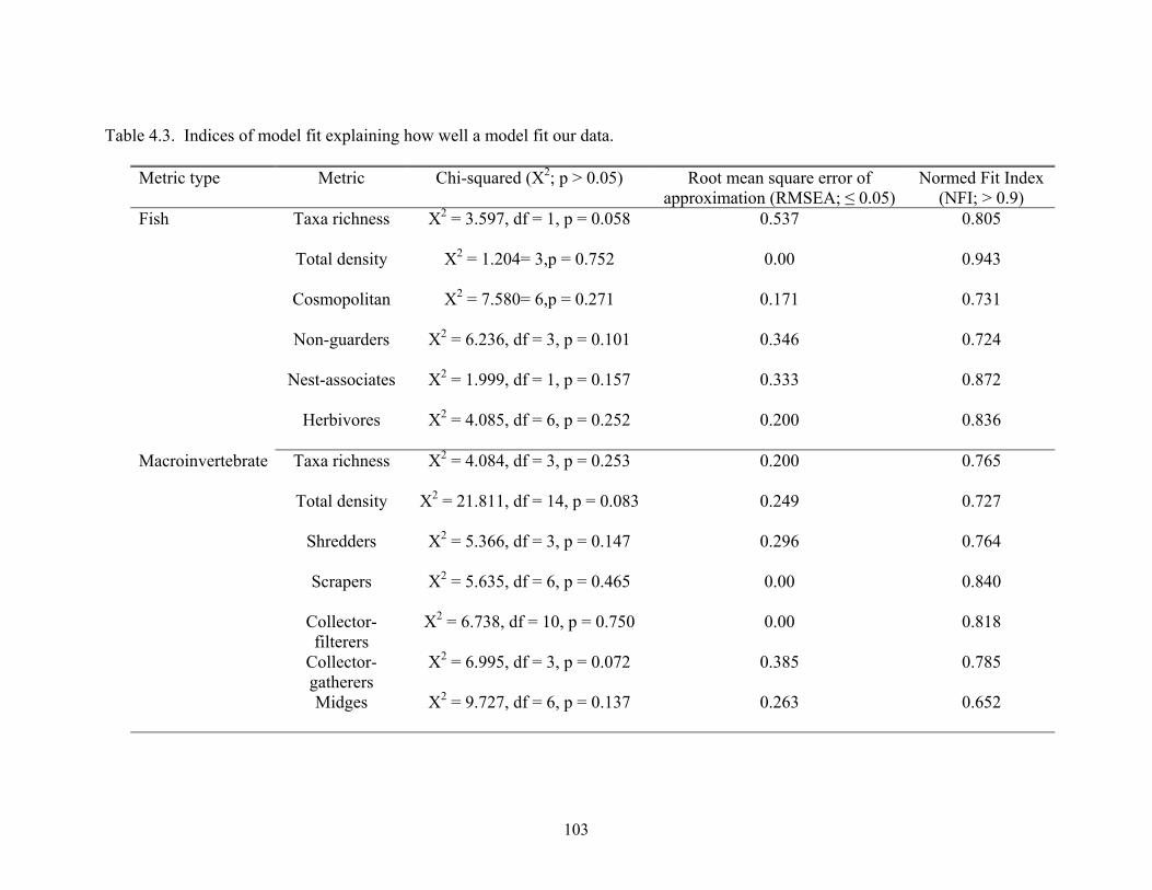
ten study streams................................................................................................................... 64 Table 3.2. Summary of mean hydrologic responses measured in ten study streams................... 65 Table 3.3. Summary of mean geomorphic responses measured in ten study streams ................. 66 Table 3.4. Summary of mean (±1SE) erosional responses measured in ten study streams ......... 67 Table 3.5. Summary of depositional responses measured in ten study streams .......................... 68 Table 3.6. Fish species collected.................................................................................................. 69 Table 3.7 Summary of fish assemblage responses....................................................................... 70 Table 3.8. List of macroinvertebrate taxa collected..................................................................... 71 Table 3.9. Summary of macroinvertebrate assemblage responses .............................................. 72 Table 4.1. Physical and biotic response with linear regression ................................................. 101 Table 4.2. Comparison of predictive ability of path models versus bivariate regression.......... 102 Table 4.3. Indices of path model fit ........................................................................................... 103

vii

List of figures

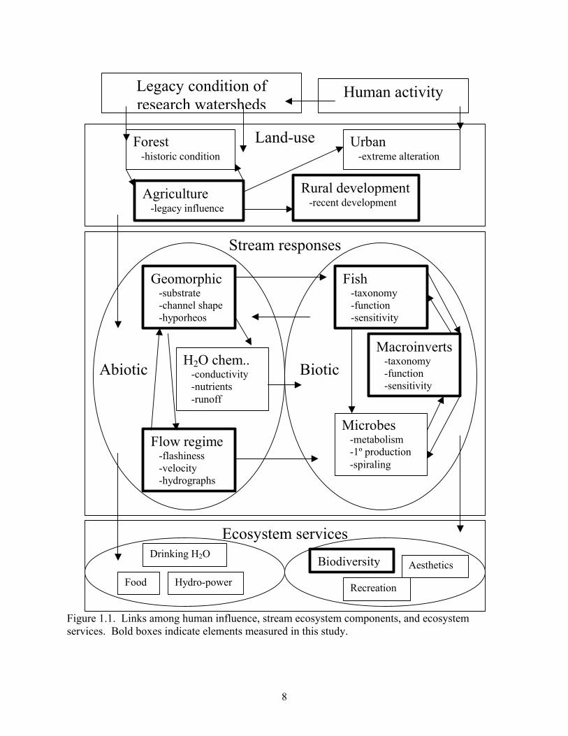
Figure 1.1. Conceptual relationships among study components.................................................... 8 Figure 2.1. Theoretical zone of influence .................................................................................... 35 Figure 2.2. Example watershed showing six travel time zones ................................................... 36 Figure 2.3. Visual comparison of zones....................................................................................... 37 Figure 2.4. Correlation between TTZs (travel time zones) and macroinvertebrate responses .... 38 Figure 2.5. Correlation between TTZs (travel time zones) and fish resposnes ........................... 39 Figure 2.6. Linear regression showing relationships between TTZ and macroinvertebrates ...... 40 Figure 2.7. Linear regression showing relationships between TTZ and fish............................... 41 Figure 3.1. Map of study area ...................................................................................................... 73 Figure 3.2. Mean (± 1 SE) TSS and FBOM concentration in rural vs. agricultural streams....... 74 Figure 3.3. Mean (± 1 SE) fish TR and NG density in rural vs. agricultural streams ................. 75 Figure 3.4. Detrended correspondence analysis of streams by fish species density.................... 76 Figure 3.5. Detrended correspondence analysis of streams by macroinvertebrate density ......... 77 Figure 3.6. Changes to abiotic and biotic stream impairment through time................................ 78 Figure 4.1. Schematic describing the general land-cover path hypothesis ................................ 104 Figure 4.2. Path diagrams reduced to include best-fit predictive models.................................. 105

viii

Chapter 1: Introduction. Stream responses to anthropogenic land-cover change

But now, says the Once-ler, Now that you’re here, the word of the Lorax seems perfectly clear. UNLESS someone like you cares a whole awful lot, nothing is going to get better. It´s not. – Theodor Seuss Geisel in The Lorax.

Stream ecosystems

Stream ecosystems are influenced by the landscapes through which they flow, and reflect

the interaction of precipitation with landscape surfaces, soil interstices, and groundwater

aquifers. Water passing through a stream reach has been exposed to, and potentially influenced

by, watershed features ranging from soil nitrifying bacteria, landscape land-cover, to

groundwater chemistry. Stream ecologists have recognized the multi-dimensional nature of

streams and that streams interact with the terrestrial environment beyond their channels. The

river continuum concept (Vannote et al. 1980) established the longitudinal nature of stream

transport. Hynes (1983) and others have recognized the hyporheic zone as defining the vertical

interaction of stream water and the semi-aquatic and terrestrial environments. Ward (1989)

added that streams are necessarily temporal and can vary within daily, annual, and geologic

periods. Contemporary stream research must address streams with respect to longitudinal,

lateral, vertical, and temporal dimensions.

Given that stream ecosystems are complex, multivariate systems that span broad temporal

and spatial scales, it becomes necessary to establish an ecologically relevant boundary within

which research efforts can be focused. Stream watersheds provide realistic boundaries of

influence that are defined by stream reaches where stream elements are measured. Ridge tops

defining drainage areas within watersheds designate the zone of influence pertinent to stream

reaches and the elements measured therein. Much of stream research has examined stream

responses at the reach or local scale and has considered that responses are influenced by

interactions occurring between stream reaches and watershed boundaries. Watersheds provide a

1

suitable framework for stream study because they span multiple spatial scales, include

longitudinal, lateral, and vertical dimensions and evoke short and long-term time scales ranging

from seconds to eons. Stream research that is focused within watersheds, therefore, assumes an

ecosystem perspective whereby researchers must consider multiple interacting variables

functioning along a broad spatial continuum.

The ecosystem perspective, however, complicates stream research due to the expansive

spatial scales, variable resource-use interests, and multiple interacting variables that researchers

and land-managers must consider (Carpenter and Kitchell 1988). In-stream variables are often

defined at the local, habitat, or patch scales (i.e., within reaches), whereas watershed scale

investigations require a landscape perspective. Stream responses can be affected at scales much

larger than those on which researchers or managers often focus. Human influence to streams

often occurs at the watershed scale, through land-use changes including agriculture or

urbanization, which occupy a large percentage of a watersheds area. However, stream responses

to anthropogenic activity are often not observable at the large scale, rather, landscape influence is

often studied by scientists or land-managers at the reach scale. Ecosystem services, such as the

provisions of drinking water or recreation, are observable somewhere within the spatial

continuum between stream reaches and landscapes. Therefore, study of anthropogenic

disturbance to streams requires an approach that spans multiple spatial scales.

Consideration of ecosystem scale disturbance requires a holistic consideration of the

stream and terrestrial environment (i.e., the watershed ecosystem). Anthropogenic activity,

current knowledge of interactions among key ecosystem elements, and an understanding of

socioeconomic goals are necessary to fully address anthropogenic disturbance to streams.

Relationships among stream responses and watershed-scale phenomena including human

activity, stream ecosystem responses, and ecosystem services are summarized in Figure 1. My

dissertation focuses on interactions among anthropogenic land-cover change, physical stream

elements, and fish and macroinvertebrate community responses.

Anthropogenic land-cover change

Streams in the southeastern United States have been influenced by human activity since

pre-European settlement (SAMAB 1996, Wear and Bolstad 1998). However, most significant

influences have been associated with post-European human manipulation of landscapes (i.e.,

2

watershed land-use) to supply consumptive services including timber harvest, agriculture, and

urban infrastructure. Humans have recently become concerned with how consumptive uses have

influenced stream structure and function.

In the eastern United States, deciduous forest has historically occupied much of the

landscape. Trees were initially harvested for direct use and to clear land for other uses, including

agriculture and urbanization. Deforestation influence to streams has been well documented, and

patterns of stream response to deforestation are predictable (Vesterby and Krupa 2001).

Removal of watershed rooted vegetation decreases soil stability and induces erosion. In-stream

sedimentation dynamics are altered by anthropogenic land-use, and often sedimentation has been

described as the most significant human disturbance to streams (Trimble and Crosson 2000).

Erosional sediments alter in-stream habitat, reduce hyporheic exchange, and decrease stream

interstices, especially when deforestation is followed by agricultural activity.

Streamside agriculture has long influenced streams in the eastern United States

(Ramankutty et al. 2002). Most streams in the eastern deciduous forest have been influenced by

a combination of deforestation and agriculture. Agriculture activity essentially perpetuates in-

stream erosion by continually disturbing watershed soils. Continual row-crop culture and

livestock grazing prevent the succession of near-stream vegetation rendering near-stream soils

susceptible to erosion. Row-crop agriculture also delivers excess nutrients and harmful

chemicals associated with fertilizer and pesticide application. Agriculture influences streams

through continual sedimentation and nutrient enrichment.

Urbanization and urban sprawl are landscape activities that also influence streams.

Roads, houses, and parking lots decrease the watershed area available to natural processes. Soil

infiltration, nutrient transformations, groundwater recharge, and other processes are interrupted

by impervious surface cover (ISC), which effectively decreases the portion of a watershed where

these processes can occur. Watershed hydraulic dynamics are often drastically altered by

urbanization as compared to other land uses (Finkenbine et al. 2000). Streams influenced by

urban activity experience higher peak flows, more frequent flooding, and greater irregularity in

flow patterns. Urban streams are also susceptible to drying and flooding extremes (Paul and

Meyer 2001).

The transformation of landscapes for rural development is an increasingly common form

of anthropogenic landscape disturbance (Kent et al. 2000). The decrease of small-scale

3

agriculture supplies formerly unavailable land for other uses including rural development. Rural

development brings roads, buildings, and sewage infrastructure to areas previously disturbed by

soil tilling, fertilizer application, and livestock grazing. Rural development is similar to urban

sprawl, but is unique because it often occurs in formerly agricultural land. Streams influenced

by rural development may continue to reflect the influence of agriculture (i.e., legacy effects

sensu Harding et al. 1998. My dissertation addresses the potential influence of rural

development on watershed ecosystems.

Dissertation goals

I investigated whether rural development influences abiotic and biotic elements in

streams that have been impaired by historical agriculture. This investigation addressed several

objectives. My first objective was to determine the extent to which rural development influenced

streams and is presented in Chapter 3. Because rural development often involves the

transformation of formerly agricultural areas, I specifically investigated whether rural

development influenced responses in southeastern U.S. streams that had been historically

influenced by agriculture.

My second objective was to develop an ecologically meaningful method for subdividing

watersheds into smaller units in which to quantify land-cover and is presented in chapter two.

Researchers have long recognized that stream reach-scale responses are differentially influenced

by not only the type of land-cover but also the location and proximity of land-cover relative to

the stream reach in which responses are quantified. Most of the progress has suggested various

methods for subdividing watersheds by distance from stream reach. For example, riparian

corridors (~30-m) have been used to define a watershed sub portion proximal to streams and

more likely to influence stream responses. Often researchers quantify land-cover in riparian

corridors and whole watersheds and use these to spatial extremes to examine the differential

probability for influence by land-cover within each area. Sponseller and Benfield (2001) used

30-m riparian corridor sections, located at various distances upstream of sample reaches, to

assess the longitudinal displacement of land-cover influence to streams. More recently, King et

al. (2005) summarized and expanded contemporary techniques for assessing land-cover at

continuous spatial scales using riparian corridors and concentric circles to subdivide research

watersheds. These types of studies have supported the idea that land-cover likely influences

4

streams along both longitudinal and lateral vectors and that the degree of influence potential by

land-cover is likely highest in an area extending upstream and outward of sample reaches.

My third objective was to link the abiotic and biotic responses I measured to land-cover

and is presented in Chapter 4. Contemporary research often suggests that land-cover influences

erosion, and that in-stream sediments influence biota. However, no study I am aware of has

successfully linked land-cover, abiotic ecosystem components, and biota, although several recent

studies have attempted to do so (see King et al. 2005). Because my investigation spanned spatial

scales from stream interstices or individual invertebrates to large watersheds, I suspected I would

be able to link responses to land-cover in watershed sub portions at various scales. One of my

most important dissertation goals was to develop and test models that summarize relationships

between land-cover, sediments, and biotic responses. Using structural equation modeling, I

identify patterns among spatial scale, land-cover, and individual stream responses (e.g., fish

diversity) that will influence future stream ecosystem research.

5

Literature cited

Carpenter, S.R., and J.F. Kitchell. 1988. Consumer control of lake productivity. BioScience

38:764-769.

Finkenbine, J.K., Atwater, J.W. and D.S. Mavinic. 2000. Stream health after urbanization.

Journal of the American Water Resources Association 5:1149-1160.

Geisel, Theodor Seuss. 1971. The Lorax. Random House, New York.

Harding, J.S., Benfield, E.F., Bolstad, P.V., Helfman, G.S. and E.B.D. Jones III. 1998. Stream

biodiversity: the ghost of land use past. Proceedings of the National Academy of Science

95:14843-14847.

Hynes, H. B. N. 1983. Groundwater and stream ecology. Hydrobiologia 100: 93–99.

Kent, M.M., Pollard, J.H. and M.Mather. 2000. First glimpses from the 2000 U.S. census.

Population Bulletin 56:1-39.

King, R.S., Baker, M.E., Whigham, D.F., Weller, D.E., Jordan, T.E., Kazyak, P.F., and M.K.

Hurd. 2005. Spatial considerations for linking watershed land cover to ecological

indicators in streams. Ecological Applications 15:137-153.

Paul, M.J., and J.L. Meyer. 2001. Streams in the urban landscape. Annual Review of Ecology

and Systematics 32:333-365.

Ramankutty, N., Foley, J.A. and N.J. Olejniczak. 2002. People on the land: changes in global

population and croplands during the 20th century. Ambio 31:251-257.

SAMAB (Southern Appalachian Man and the Biosphere). 1996. The Southern Appalachian

assessment social/cultural/economic technical report: report 4 of 5. Atlanta: US

Department of Agriculture, Forest Service, Southern Region.

Sponseller, R.A., and E.F. Benfield. 2001. Appalachian headwater streams: a multiple-scale

analysis. Journal of the North American Benthological Society 20:44-59.

Trimble, S.W and P. Crosson. 2000. U.S. soil erosion rates – myth and reality. Science

289:248-250.

Vesterby, M. and K.S. Krupa. 2001. Major Uses of land in the United States, 1997. Resource

Economics Division, Economic Research Service, USDA. Washington, D.C. Statistical

Bulletin No. 973. 47 pps.

Ward, J.V. 1989. The 4-dimensional nature of lotic ecosystems. Journal of the North American

Benthological Society 8:2-8.

6

Wear, D.N., and P. Bolstad. 1998. Land-use changes in southern Appalachian landscapes:

Spatial analysis and forecast evaluation. Ecosystems 1:575-594.

Vannote, R.L., G.W. Minshall, K.W. Cummins, J.R. Sedell, and C.E. Cushing. 1980. The river

continuum concept. Canadian Journal of Fisheries and Aquatic Sciences 37:130-137.

7

Figure 1.1. Links among human influence, stream ecosystem components, and ecosystem services. Bold boxes indicate elements measured in this study.

Legacy condition of research watersheds

Human activity

Land-use

Stream responses

Ecosystem services

Rural development -recent development

Urban -extreme alteration

Agriculture -legacy influence

Forest -historic condition

Geomorphic -substrate -channel shape -hyporheos

H2O chem.. -conductivity -nutrients -runoff

Flow regime -flashiness -velocity -hydrographs

Microbes -metabolism -1º production -spiraling

Macroinverts -taxonomy -function -sensitivity

Fish -taxonomy -function -sensitivity

Biodiversity Aesthetics

Recreation

Drinking H2O

Hydro-powerFood

Abiotic Biotic

8

Chapter 2: Defining spatially explicit riparian zones using watershed hydrology Abstract

Riparian zones have been identified as areas where the terrestrial landscape can

disproportionately influence streams. However, defining riparian zones is complicated for

several reasons. Near-stream areas represent dynamic spatial gradients, or zones, characterized

by varying, topography, geology, land-cover, and the degree of terrestrial – aquatic interaction.

Many studies have considered these influence zones to be discreet watershed sub-portions (e.g.,

100-m riparian corridors), whereas I consider zones of influence to be composed of multiple

watershed sub-portions along the spatial continuum between near-stream areas and the watershed

boundary. I describe a method for identifying zones of influence using watershed hydrologic

patterns to delimit zones along a near-stream continuum between a downstream point (e.g.,

sample reach) and the watershed boundary. Using hydrologic modeling equations and GIS,

travel time zones for ten streams were identified by watershed topography, surface roughness,

and rainfall intensity. Travel time was calculated for every 30 X 30-m cell in each watershed,

providing spatially explicit estimates of watershed hydrology and enabling us to calculate the

travel time required for rainfall in any watershed cell to reach the watershed terminus, or stream

reach. Mean watershed travel time varied from 45 to 264 minutes among ten watersheds.

Shorter duration travel times (i.e., 30 – 60 minutes) described smaller areas than longer duration

travel times (i.e., 210 – 300 minutes). Travel time zones were wider and shorter than traditional

riparian corridors and described areas more ecologically relevant to stream reaches. I used

correlation to assess the ‘best’ zone to use when defining disturbance type land cover influence

on common biotic responses. Macroinvertebrate shredder and midge density were related to

heavy and light urban land-cover defined within travel time zones between 90 and 240-min.

Benthic invertivores and nest-associate fishes were also correlated to urban land-cover delimited

by zones. Travel time zones were better (i.e., higher correlation coefficient and r2) at detecting

biotic responses than 100-m riparian buffers. This method provided a framework for analyzing

landscape condition in continuous riparian zones that allowed comparison of ecologically

relevant land-cover with response variables at multiple spatial scales.

9

Introduction

Streams are influenced by upstream factors associated with landscape condition (Wiens

2002). Studies of landscape - stream interactions are important for natural resource

conservation, insightful land management, and understanding ecosystem structure and function.

Researchers have often considered aspects of landscape condition (e.g., land-cover) to be

influential determinants of physical, chemical, and biotic stream responses (Roth et al. 1996,

Trimble and Crosson 2000). Multiple lines of evidence suggest that streams are affected by

landscape condition (e.g., anthropogenic disturbance) and that stream responses are directly

related to the type, intensity, and location of landscape disturbance factors (Gupta 1995, Gomi et

al. 2002, Woessner 2000, Montgomery and MacDonald 2002). Most research has suggested that

riparian zones are key areas that mediate the effects of landscape disturbance to streams

(Friedman et al. 1996, Croke et al. 1999, Paringit and Nadaoka 2003).

Riparian zones are critical ecosystem components located at the terrestrial – aquatic

interface (Decamps et. al 1988, NRC 2002, Moore and Richardson 2003). A wealth of evidence

suggests that this near-stream environment mediates disturbance to stream ecosystems and that

riparian zones are disproportionately sensitive to anthropogenic disturbance (Karr and Schlosser

1978, Decamps et. al 1988, Gregory et. al 1991, FIWG 1998, Naiman et. al 2001, Molnar et al.

2002). However, appropriate spatial boundaries that define riparian zones are not well

understood. Consequently, there are multiple ways to describe riparian zones with respect to

both the landscape and streams (Postel et. al 1996, Stanford 1998, COS 1999). Most define

riparian zones as areas of terrestrial – aquatic interaction but disagree as to where to place

boundaries. Researchers, land-managers, and ultimately, policy decision-makers often define

riparian zones by criteria such as distinctive vegetation, periodic flood boundaries, or

topographic features (NRC 2002). Many contemporary studies have defined riparian areas as

uniform-width (e.g. 100-m buffer) corridors (e g. Harding et al. 1998, Sponseller and Benfield

2001, Boothroyd et. al 2004, Lee et. al 2004). Most longitudinal analyses of streams, however,

have indicated that lateral inputs become more important moving downstream, which suggests a

non-uniform width of the riparian zone (e.g., Vannote et. al 1980, Montgomery 1999, Molnar et

al. 2002). At minimum, riparian boundaries should vary with stream size and across

physiographic provinces.

10

Researchers have demonstrated the need to consider multiple spatial scales when

investigating stream responses to landscape disturbance (Smart et al. 2001, Wiens 2002,

Townsend et al. 2003, King et al. 2005). Recent investigations have used exploratory methods to

define riparian zones along spatial continua to allow comparison of stream responses with

landscape condition at several spatial scales (Basnyat et al. 1999, Smart et al. 2001, Sponseller

and Benfield 2001, Apan et al. 2002, Reed and Carpenter 2002, Townsend et. al 2003, Hyatt et

al. 2004, Lee et. al 2004, King et al. 2005). These studies differ in how they consider spatial

scale, but all aim to quantify near-stream areas that are spatially and ecologically relevant

riparian zones and to use these zones as areas to focus their description of landscape condition.

Given that riparian zone boundaries differ among systems, a standard definition should be a set

of dynamic criteria used to define riparian zones in individual systems. This would allow for

objective comparison among and between streams of various types. At present, the lack of a

standard riparian definition limits our ability to associate landscape condition with detrimental

stream responses, inhibits unified research across disciplines and lengthens the time required to

make ecologically beneficial decisions (Steiner et. al 1998).

Here I present a method for delimiting multiple riparian zones of varying size around

stream channels using surface hydrologic characteristics. King et al. (2005) suggested that

hydrological connectivity should be considered when sub-dividing watersheds for land-cover

analysis. Hydrologic features are useful because water, via the hydrologic cycle, unites streams

with terrestrial landscapes (Gordon et. al 2004, McKergow et al. 2004). Riparian zones defined

by hydrologic pathways include gradients from wet (i.e., streams) to dry (i.e., upland terrestrial)

areas. Hydrologic patterns can be quantified and used to identify and describe spatially

continuous, ecologically relevant riparian zones. In this chapter, I summarize watershed

hydrology using estimates of watershed travel time, or the average time required for rainwater

resulting from a uniform watershed rainfall to travel between any specified portion of the

landscape and a typical stream reach.

The first objective of this study was to use travel time estimates to define continuous

watershed sub-portions, or zones, along the spatial continuum from near-stream to the whole

watershed. I used travel time to delimit ecologically different and spatially explicit watershed

sub-portions or riparian zones. My second objective was to use travel time zones (TTZs) to

describe land-cover characteristics in watershed sub-portions. I predicted that land-cover would

11

differ with the TTZ in which land-cover was delimited and provide a way to consider land use at

multiple spatial scales. My third objective was to use TTZs to determine the appropriate spatial

scale of land-cover that influenced each biotic response. I predicted that some responses would

be related to (i.e., stronger correlation) to land-cover at larger spatial scales (i.e., longer duration

TTZs) whereas other responses would be related to land-cover at smaller (i.e., more proximal,

shorter duration TTZs) spatial scales. To address objective three, I compared land-cover

described in multiple travel time zones to abiotic and biotic responses to determine the

appropriate zone, and spatial scale, relevant to each response.

Methods

Conceptual approach

I used hydrologic dynamics as criteria to define spatially explicit riparian zones in

disturbed watersheds because hydrologic dynamics address interactions between water,

terrestrial areas, and stream channels and can be defined along a spatial continuum (Gupta 1995,

Friedman et al. 1996, Walling 1998, Croke et al. 1999, Gomi et al. 2002, McKergow et al. 2004,

Melesse and Graham 2004, Vidon and Hill 2004). I predicted that hydrologic estimates would

describe watershed sub-portions resembling the zone described in Figure 2.1. Watershed

hydrology results from rainfall flowing toward stream channels along lateral and longitudinal

vectors. Hydrologic patterns define the watershed area where surface terrestrial – aquatic

interaction are likely to occur (Fig. 2.1; Ward 1989, Smock et al. 1992) and describe a continuum

of terrestrial – aquatic interaction. Areas within the riparian continuum that are closer to streams

should reflect a higher degree of terrestrial – aquatic coupling than less proximal, more terrestrial

areas. Near-stream areas are zones of influence and are more likely to introduce eroded soils or

other artifacts of disturbance to stream channels during a typical rainfall than are less proximal

areas.

I used travel time thresholds to delimit watershed sub-portions that were organized by the

maximum travel time occurring in an area. Thus, TTZs were identified by the relative amount of

terrestrial – aquatic interaction as defined by common travel times. Watershed sub-portions with

similar travel time estimates could therefore be grouped into a TTZ. In this study, watershed

sub-portions were composed of 30 X 30-m cells designated by GIS software. My models

calculated the time required for uniform rainfall in a cell to travel to the nearest stream channel

based on modeled landscape parameters including gradient, surface roughness, and proximity to

12

a stream reach or watershed outlet. Travel time zones represented the grouping of cells similar

in the travel time required for rainfall to reach a stream channel. For example, a 60-min travel

time zone would include all watershed cells where rainfall reached a stream channel within 60

minutes. Similarly, 60-min TTZs would be characterized as having a smaller area, being

generally closer to a stream reach or watershed outlet, and having less terrestrial – aquatic

interaction than a 120-min travel time zone. However, 120-min TTZs would include the 60-min

TTZs and all other shorter-duration TTZs. Increasing the duration of a TTZ, therefore, involved

adding new cells to the next-smaller TTZ. Potential riparian areas were thus defined by a

continuum of short to long duration travel times with short duration travel times representing

local, near-stream watershed spatial scales and longer duration travel times representing

successively larger watershed areas.

Research watersheds

Travel time estimates were calculated for each 30 X 30-m cell (900-m2) in ten example

watersheds (Table 2.1). I focused on watersheds disturbed by agriculture, averaging 23 ± 5.6 %

( x ± SE; range: 16 – 36%) row-crop agriculture. Watersheds were located in the Blue Ridge

physiographic province of the southern Appalachians near Asheville, NC. Watersheds were

similar size, ranging from approximately 900 – 3500 hectares ( x = 1898 ha), contained similar

stream networks (7 – 28 km) featuring streams of 3rd – 4th order at the watershed outlet, occurred

at approximately 2000 m elevation, and shared similar soil characteristics. The ten watersheds

were considered comparable replicates and used to examine the variation in watershed areas

prescribed by TTZs, 100-m corridors, and whole watersheds.

Hydrologic Equations and GIS

Stream networks were delineated and stream slope estimated using ESRI® ARCGIS®

version 8.2, the spatial analyst extension, and 30-m digital elevation models obtained via the

USGS seamless data distribution website*. Flow direction, accumulation, stream networks and

watershed boundaries were delineated in ARCGIS® using the hydrology extension. Streams

were truncated at flow accumulations of 250 cells to define the boundary between ephemeral and

perennial flow and included only perennial flow (Saunders 2000). Land-cover estimates were

obtained from National Land Cover Database (NLCD) and used to calculate surface roughness

(EPA 2000; Homer et. al 2002). Twenty-seven NLCD land-cover categories present in study

*http://www.seamless.usgs.gov/

13

watersheds were collapsed into seven general groups due to limited availability of roughness

coefficients (n) for specific land-cover types (Table 2.1). Because accurate estimates of n are

not known for many land-cover types, I estimated n for unknown categories by extrapolating

between known n values for intermediate land-cover types.

I used HEC-HMS equations developed by the US Army Corps of Engineers to quantify

surface water velocity resulting from an average rainfall (assuming uniform rainfall in every

watershed cell; USACE 2000). While HEC-HMS equations were developed to estimate

overland flow velocity, I use travel time estimates as proxy measures of relative travel time to

weight watershed sub-portions. These are standard equations commonly used to calculate water

velocity resulting from storms of various intensities. Three types of flow were included in the

analyses: Sheet flow (sf), concentrated flow (cf), and channel flow (ch). Sheet flow occurred

along steep gradients, over impervious surfaces, or in ephemeral drainages changing to

concentrated flow after 100-m (USACE 2000). Concentrated flow occurred throughout most of

a watershed prior to water reaching a stream channel. Channel flow resulted from water entering

stream channels. The following HEC-HMS equations were used to estimate these parameters

(USACE 2000):

sf travel time = 0.42 (n * L)0.8

L(m) * P0.5 * S0.4

cf travel time = 1 / (sqrt(S) * 295.2)

ch travel time = n / 60-min * R2/3 * S1/2

where n was Manning’s roughness coefficient for each land-cover type (sensu Zelinski and

Quackenbush 1999; Table 2.1), L was the distance from stream channel (m), P was the rainfall

estimate modeled (0.5-in for this study, assumed to be equivalent for each watershed cell), S was

the slope over which water traveled and R was the estimated hydraulic radius of the stream

channel. Constants were derived from HEC-HMS equations.

Travel time was calculated using the Spatial Analyst® raster calculator and produced

spatially explicit GIS grids comprised of 900-m2 cells with values defined as the travel time

required for water to flow between that spatial location and the watershed outlet point. Velocity

estimates (m min-1) were reciprocated (min m-1) as the time required for surface water to travel

14

one meter to allow consideration of the relative time required for a parcel of water to reach the

watershed terminus, rather than the velocity of that water parcel. This rate was calculated for

every watershed cell (30 X 30-m), estimating the time required for rain falling into that cell to

reach a stream channel and ultimately the watershed outlet. Flow paths were determined by

elevation differences estimated from digital elevation models (DEM). Therefore, each cell along

a flow path would have a unique travel time estimate depending on the characteristics of

accumulating cells along that flow path. The total distance of a cell (m) to the watershed outlet,

as defined by the flow path, was equivalent to a travel time estimate (min) for that cell. Finally,

watershed sub-portions were defined by common travel time values, or thresholds, producing

zones characterized by similar travel time characteristics and thus a similar degree of terrestrial –

aquatic interaction. For example, a 30 – 60-min TTZ described the watershed sub-portion where

flow required between 30 and 60-min to reach the outlet.

Land-cover and biotic responses

I used TTZs to assess variability in land-cover estimates in seven NLCD land-use

categories (Table 2.1), and compared percent land-cover among TTZs, 100-m corridors, and

whole watersheds using analysis of variance. I used estimates of fish and macroinvertebrate

diversity as potential responses to land-cover to explore potential differences in biotic responses

with land-cover as delimited by TTZs (i.e., spatial influence). Quantitative (Surber, 500 µm

mesh) samples were collected in April 2001 and I calculated macroinvertebrate taxa richness

(total number of taxa collected), density (number of individuals collected divided by sample

area), and Simpson’s diversity index (D = (n/N)2, where n = density of taxa n, and N = total

density of all taxa combined). Further, I quantified total macroinvertebrate density and the

density of macroinvertebrates by functional feeding group (FFG; Merritt and Cummins 1996;

Table 2.4). Fish taxa richness was calculated from quantitative fish samples collected during

August 2002 by single-pass backpack electrofishing of 1 to 10-m stream reaches included within

a 100-m sample reach. Other fish metrics, including density by trophic and reproductive guilds,

were used to examine potential differences in fish assemblages with respect to taxonomy and

links between reproductive and feeding behavior linked to habitat availability (Table 2.2).

Trophic and reproductive habits were assigned according to literature available on individual

species dietary constituents and reproductive habitat preference (Jenkins and Burkhead 1994,

Etnier and Starnes 1993). When macroinvertebrate or fish taxonomic information was not

15

available, expert opinion was applied to place individual taxa into the most appropriate

functional group or guild.

To address the influence of spatial scale as estimated by TTZs on the relationship

between land-cover and biotic responses, I compared the degree of relatedness (e.g., correlation)

between each TTZs for every biotic response measured using Pearson correlation (SigmaStat v.

3.0, SPSS, Inc). I compared the correlation coefficient (r value) and correlation direction (i.e.,

positive or negative) against each TTZ to determine the ‘best’ TTZ indicated for a particular

biotic response, as indicated by the strongest significant correlation. Through these analyses I

identified the most relevant spatial scale at which land-cover had the greatest potential to

influences a biotic response. Land-cover proportions were arcsine-root-transformed, and

Simpson’s index was log-transformed to meet normality assumptions necessary for linear

regression (Zar 1999).

Results

Mean watershed travel time varied from 45 to 264 minutes (Table 2.3). Maximum travel

time in any watershed (n = 10) varied from 257 to 1,973 min (Table 2.3). Within this range of

whole watershed travel times, I was able to define TTZs by ten travel time thresholds; 30, 60, 90,

120, 150, 180, 210, 240, 270, and 300 minutes (Fig. 2.2). The smallest and largest TTZs,

defined by 30-min (0.5-hr) and 300-min (5-hr) travel time, respectively, represented realistic

endpoints for observed storms in the Asheville, NC vicinity (C.L. Burcher, personal

observation).

Travel time zones

The spatial extent of a TTZ increased with travel time (i.e., longer duration TTZs covered

successively larger watershed portions and included all smaller TTZs; e.g., Fig. 2.2). These

patterns show that TTZs describe a continuous watershed sub-portion originating at the

watershed outlet and becoming successively larger in area with increased travel time (Fig. 2.3).

Each successively larger TTZ included the areas circumscribed by all shorter-duration TTZs

(e.g., a 60-min TTZ would be within a 120 minute TTZ). I assumed that watershed areas

remained wet, and thus, connected, through the duration of modeled rainfall.

Short-duration (30 to 60-min) TTZs encompassed, on average, less than 20 percent of

watershed area (Table 2.3) and included areas lateral to stream channels but did not describe

upstream areas to the same degree as longer-duration TTZs. Intermediate-duration (90 to 180

16

minute) TTZ coverage ranged from 37 to 68 percent watershed area (Table 2.4). Long-duration

TTZs (210 - 300 minute) included 74 to 90 percent of watershed area on average, approaching

the area defined by the whole watershed (Table 2.3). Long-duration TTZs covered watershed

areas both farther upstream of and farther laterally to the watershed outlet compared to short-

duration TTZs. One-hundred-meter riparian corridors occupied 3 to 4 % watershed area ( x ± SE

= 4.0 ± 0.0 %) although they included the watershed portion extending to the extreme

headwaters but described a lateral area only 50-m on either side of stream channels. Variation

(standard error) among sites ranged from 4 to 11 percent for TTZs, whereas 100-m riparian

corridors and whole-watersheds exhibited low variation (SE = 0.0 %; Table 2.3).

Areal coverage by TTZs differed from 100-m corridor coverage (Fig. 2.3). Travel time

zones described much wider areas than 100-m corridors. Sixty minute and larger TTZs

described a larger watershed sub-portion than 100-m corridors in all watersheds. Travel time

zones also increased downstream with travel time duration, typically converging on 100-m

corridors beyond 300-min. In general, 100-m corridors were much narrower and much longer

than TTZs and delimited a smaller area than TTZs except for 100-min TTZs in four watersheds

that delimited 1 to 3 % watershed area.

Land-cover and TTZs

Agriculture, forest, and barren land-cover proportions varied significantly when

described at different spatial scales (i.e., using different TTZs; Table 2.4). Agriculture and forest

proportions in short-duration TTZs (i.e., 30 to 90-min) were similar to agriculture and forest

proportion delimited by 100-m corridors but significantly different from the proportion delimited

by intermediate to long duration TTZs (120 to 300-min) and whole watersheds. Although not a

disturbance-type land-cover, the proportion of barren areas also differed significantly with zone

whereby 30-min TTZ and 100-m corridor (i.e., small scale) land-cover estimates were different

from barren land-cover delimited by 60 to 300-min TTZs or whole watersheds (i.e., large scale).

Land-cover proportions in other categories (i.e., open water, light and heavy urban, and riparian

vegetation) did not differ significantly by zone.

Biotic responses; selecting the appropriate TTZ

Correlations between disturbance type land-cover in each TTZ (agriculture, light urban,

heavy urban) and biotic responses were used to select the most appropriate, or most predictive,

TTZ for a given biotic response. I used Pearson product moments (SigmaStat v. 3.0, SPSS Inc.)

17

to estimate the magnitude and direction of relationships between each biotic response and

disturbance type land-cover within 30 to 300-min TTZs. Light and heavy urban land-cover

types were significantly related to several macroinvertebrate and fish responses. Shredder

density was positively correlated to both light and heavy urban land-cover (Fig. 2.4A,B) and

midge density was positively correlated to light urban land-cover (Fig. 2.4C). Light urban land-

cover was most predictive when prescribed within a 150-min TTZ and heavy urban land-cover

was most predictive when prescribed within a 90-min TTZ (Fig. 2.4). The seven other

macroinvertebrate metrics were not significantly correlated to land-cover as described by TTZs,

100-m corridors, or whole watersheds. Two of thirteen fish metrics were significantly correlated

to disturbance type land-cover within TTZs. Nest associate density was most strongly predicted

(negative relationship) by light urban land-cover within 240-min TTZs and benthic invertivore

density (positive relationship) by heavy urban land-cover within 120-min TTZs (Fig. 2.5A,B).

Other fish metrics were not significantly correlated to disturbance type land-cover, and no biotic

responses were significantly correlated to agriculture.

The predictive value of strongly correlated TTZs was further assessed using linear

regression of the most significant correlated TTZ – biotic response relationships. Light urban

land-cover in 150-min TTZs significantly predicted midge density (Fig. 2.6A) and shredder

density (Fig. 2.6B). Shredder density was also strongly predicted by heavy urban land-cover

within 90-min TTZs (Fig. 2.6C). Similarly, fish nest associate density was strongly predicted by

light urban land-cover within 240-min TTZs (Fig. 2.7A) and benthic invertivore density by

heavy urban land-cover within 120-min TTZs (Fig. 2.7B). Significant biotic responses were best

predicted by disturbance type land-cover prescribed in intermediate to long duration (i.e., 90 to

240) TTZs.

TTZs vs.100-m riparian buffers

I assessed the relative value of TTZs compared to traditional 100-m buffer zones using

the significant relationships above. TTZs always out performed 100-m corridors as interpreted

by consistently higher correlation and regression coefficients (Table 2.5). Relationships between

heavy urban land-cover to shredders and light urban land-cover to nest associates were not

significant when land-cover was delimited by riparian corridors. Though highly correlated, land-

cover prescribed within TTZs predicted biotic responses better than 100-m riparian corridors.

18

Discussion

Travel time zones

Spatially explicit travel time estimates provided a useful method to define continuous

watershed sub-portions resembling my hypothesized zones of influence (Fig. 2.1). Travel times

increased moving away from streams and provided an objective method to weight watershed

sub-portions with respect to potential influence of landscape features on streams. Stream

ecologists have long recognized the lateral and longitudinal nature of streams, that streams are

influenced by material transport, and that researchers should consider lateral, longitudinal, and

vertical dimensions (sensu Vannote et al. 1980, Ward 1989, Smock et al. 1992), and recent

studies of land-cover influence on streams have explored inverse distance weighting (IDW) and

other weighting schemes to account for potential changes to landscape influence with distance

from streams (King et al. 2005). Weighting techniques, however, are not based on ecologically

meaningful criteria but instead define the linear distance from a landscape area to a stream reach.

Travel time zones reflect the lateral and longitudinal movement of water through the terrestrial

environment to stream channels. These results provided a quantitative method to assess how

landscape influence may be translated downstream-of and lateral-to a terrestrial location.

Continuous riparian zones allow for considering lateral and longitudinal interactions with respect

to sample locations. TTZs provide an appropriate method to evaluate the influence of scale

relative to the types of responses measured.

Areal variation among zones was highest for short-duration TTZs (i.e., near-stream

zones) compared to zones occupying larger portions of watersheds. While this is a subtle

difference, it could suggest that near-stream areas are more likely to vary in size or travel time

duration than less-proximal watershed areas. This observation agrees with the variable source

concept that suggests near-stream areas disproportionately influence stream channels (Hewlett

and Hibbert 1967). Similarly, variation in intermediate TTZs suggests that watershed areas

between ridge tops and stream valleys are most likely to vary with respect to the type of land-

cover present.

Biotic responses

As I predicted, biota were influenced by disturbance land-cover at some spatial scales

(i.e., within some TTZs) but not others. Researchers have addressed the differential effects of

spatial scale on biotic responses associated with land-cover spatial distribution (Harding et al.

19

1998, Sponseller and Benfield 2001, King et al. 2005), although I am not aware of other studies

that used hydrology or other ecologically meaningful criteria to establish spatial gradients. Here,

TTZs were successful in showing differential effects of land-cover at various spatial scales.

Additionally, differences in biotic responses to land-cover at varying spatial scales suggests that

studies relying solely on whole watershed or corridors to delimit land-cover may miss potentially

meaningful relationships. For example, shredder density in my study streams was influenced by

heavy urban land-cover within 90-min TTZs, but not by heavy urban land-cover prescribed by

100-m buffers. Had I used traditional methods, I would not have observed the potential

influence of urban land-cover to shredder density.

Heavy and light urban land-cover types delimited by 90 to 240-min TTZs were most

significantly related to the biotic responses we measured, whereas agriculture was not.

Agriculture has been inferred as a likely influence on many of the biotic responses we measured,

but neither TTZs nor traditional methods of land-cover suggested that agriculture was related to

biotic responses in the streams we studied. Although agricultural land-cover dominated

watersheds, our results suggest that urban land-cover types may be more influential to biota in

these streams. Several researchers have suggested that urban land-cover types are more

detrimental to streams than agriculture, and it is likely that we observed a similar phenomenon

(Paul and Meyer 2001). Streams in the southern Appalachians have likely been influenced by

agriculture for hundreds of years, and biotic assemblages may reflect acclimation to conditions

induced by agriculture (Harding et al. 1998). Urban development in the study area is recent

compared to agriculture, and we may have observed the response of assemblages to ‘unfamiliar’

disturbance influence.

Urban land-cover was positively correlated with both shredder and midge density.

Shredders are organisms relying largely on allocthonous input of food associated with autumnal

leaf fall in the eastern United States. Tipula (Diptera) and Frenesia (Trichoptera) dominated

developing streams but were absent from agricultural streams. Increased shredder density with

urban land use suggests that riparian vegetation is recovering in urban streams compared to

agricultural areas. This is possible because agricultural streams typically contain denuded

riparian areas, bare banks, and minimal allocthonous input, whereas urban systems do not

necessarily feature denuded stream banks. However, we also observed increases to midge

density associated with urban land-cover. Typically, midges are considered tolerant to pollution

20

and often are associated with impairment. That midges and shredders both increased with urban

land use may therefore be contradictory. We did not, however, attempt to identify midges past

family, which may be causing confusion in the interpretation of these results.

Urban land-cover also influenced fish assemblages. Benthic invertivore density

increased with urban land-cover and nest associate density was negatively correlated to urban

land-cover. Benthic invertivores typically have down-turned, or subterminal, mouths and may

be associated with feeding on benthic invertebrates (Jenkins and Burkhead 1994). The increase

of benthic invertivores suggests that prey items (i.e., macroinvertebrates) associated with benthic

areas were readily available. Correlation of benthic invertivores with urban land-cover may

suggest that conditions in the benthos were improved over streams influenced by agriculture.

However, nest associate fishes tended to decrease in abundance with urban land-cover. Nest

associates prefer to spawn in association with nest-building fish species including stonerollers

and creek chubs. It is possible that altered watershed hydrology often associated with urban

land-cover may reduce the success of the nest building and nest associate spawning strategies.

Alterations to fish assemblages associated with urban land use suggests that rocky habitats and

substrate conditions are influenced by urban land-cover, and that these changes may be

influencing fish feeding and reproductive habits. Moreover, altered stream conditions likely

favor fishes adapted to or able to acclimate to, substrate condition.

Ultimately, macroinvertebrate midge and shredder density and fish benthic invertivore

and nest associate density were most related to urban land-cover described by intermediate to

long-duration TTZs (i.e., 90 to 240-min). This is an indication that urban land cover at moderate

to large spatial scales (i.e., including near stream and middle watershed areas, but not areas

closer to the watershed boundary or farther away from stream reaches) is disproportionately

influential to assemblages compared to other land-cover types or either near stream or large-scale

urban land-cover. Despite the relatively small contribution of urban land-cover and the

dominance of agriculture in watersheds (Table 2.1), biota appeared to be influenced only by

urban land-cover. This suggests that urban land-cover induces a disproportionate influence on

biota compared to agriculture, and that a large spatial scale (i.e., larger than 100-m corridors

provide) should be considered when investigating assemblages potentially influenced by urban

land use.

21

Selecting the appropriate TTZ

Variation in the proportion of land-cover delimited by TTZs suggested an effect of spatial

scale. Peaks in response curves generated by correlations between biotic responses and TTZs

indicated that urban land-cover defined between 90 and 240-min were most predictive and

potentially highly influential on biota. Correlation analysis can be used in conjunction with

TTZs to determine the appropriate area to consider when making management decisions. Many

investigations, public projects, and management efforts need to assign the relevant sub-

watershed area that is critical to respective criteria. For example stream management for Total

Maximum Daily Loads (TMDLs) requires knowledge about the origin of sediments in order to

successfully manage sediment delivery to streams. Using TTZs together with in-stream

sediment sampling managers can focus efforts on land-cover types or other sub watershed

criteria significantly related to sediment concentration. Travel time zones provide an

ecologically relevant technique for subdividing watersheds along a spatial continuum and

determining which of the subdivisions is most related to the management parameter of interest.

Further consideration

While travel time estimates appeared to provide insight regarding the relationship

between land-cover and spatial scale for these watersheds, whether the selected equation

parameters would be appropriate for other watersheds is unknown. It is difficult to validate

spatially explicit models considering the inconsistent nature of rainfall and difficulties of

empirically testing watershed hydrology. Potential error in travel time estimates depends on the

accuracy of appropriate equation parameters and the nature of watershed hydro-dynamics.

Several aspects of the selected equation terms merit future exploration to address questions of

accuracy. For example, Manning’s roughness coefficients have not been verified for land-cover

types. Our estimates of n were based on available data, although the actual resistance supplied

by each land-cover type is not well understood. I addressed potential circularity in using land-

cover to estimate n, and deriving land-cover zones using travel time using linear regression. If n

estimates disproportionately affected travel time estimates, travel times should have increased

with forest cover and decreased with agriculture because forest cover was assigned a much

higher n value relative to agriculture. Higher n values, theoretically, could have increased travel

times due to increased surface roughness impeding water flow. Had travel time estimates been

unrealistically long (e.g., 10,000 minutes), and could have been attributed to n values, I would

22

have reconsidered the n estimates used. Instead, I found that maximum travel time was

positively associated with higher forest cover and negatively associated with higher agriculture

in whole-watersheds. I considered this evidence that equations were not circular with respect to

land-cover and n estimates. Similarly, this suggested that equations were not influenced greatly

by n.

Other parameters that could create error include the digital elevation model (DEM)

derived hydrology calculated in GIS. Several researchers have demonstrated errors associated

with locating stream networks with DEMs, especially in low-gradient areas (Wang and Yin,

1997, Yin and Wang 1999, Moglen and Beighley 2002). Digital elevation model derived slope

estimates also may not reflect true hillslope orientation and stream channel locations may differ

subtly from actual locations. Similarly, the resolution of DEMs and land-cover data was 30-m

(30 X 30-m cells). As a result, stream channels and hydrologic vectors were estimated to be

much larger than they were. These potential problems may over or under estimate travel time

calculations. Equations were selected to summarize watershed features believed to be important

in these systems. Using travel time to define the extent of riparian zones worked well in

disturbed 3rd – 4th order southern Appalachian streams. Whether larger watersheds, low-gradient

streams or groundwater-dominated systems could be similarly analyzed is unknown. Researchers

working in other streams should include the features important in those areas in equations.

Conclusion

Investigations of stream reach-scale responses to landscape condition could benefit from

a spatially explicit consideration of the landscape (King et al. 2005). Here I present a conceptual

approach that can be used across geographic, geologic, and elevation gradients. Using TTZs to

define zones of influence is an accurate and appropriate method for use in disturbed watersheds

with increased hydrologic activity. Future research can now consider stream responses to

landscape condition defined at multiple spatial scales within continuous riparian zones. I suggest

that research comparing in-stream responses to landscape condition should consider using travel

time or similar spatially continuous hydrologic estimates to define land-cover as an independent

variable for comparison with stream responses. This is one of the first studies suggesting the use

of continuous spatial zones to define zones of influence. Further research will help modify

equations to change the important parameters, reduce the necessary GIS estimates or the

23

associated error, improve estimates of roughness coefficients, and potentially validate travel time

estimates to determine accuracy.

24

Literature Cited Apan, A.A., S.R. Raine, and M.S. Paterson. 2002. Mapping and analysis of changes in the

riparian landscape structure of the Lockyer Valley catchment. Queensland, Australia.

Landscape and Urban Planning 59:43-57.

Basnyat, P., L.D. Teeter, K.M. Flynn, and B.G. Lockaby. 1999. Relationships between

landscape characteristics and nonpoint source pollution inputs to coastal estuaries.

Environmental Management 23:539-549.

Boothroyd, I.K.G., J.M. Quinn, E.R. Langer, K.J. Costly, and G. Steward. 2004. Riparian

buffers mitigate effects of pine plantation logging on New Zealand streams 1. Riparian

vegetation structure, stream geomorphology, and periphyton. Forest Ecology and

Management 194:199-213.

Committee of Scientists (COS). 1999. Sustaining the people’s lands: Recommendations for

stewardship of the National Forests and Grasslands into the next century. Washington,

D.C., U.S. Department of Agriculture.

Croke, J., P. Hairsine, and P. Fogarty. 1999. Runoff generation and re-distribution in logged

eucalyptus forests, south-eastern Australia. Journal of Hydrology 216: 56-77.

Decamps, H., M. Fortune, F. Gazelle, and G. Pautou. 1988. Historical influence of man on the

riparian dynamics of a fluvial landscape. Landscape Ecology 1:63-73.

EPA [United States Environmental Protection Agency]. 2000. Multi-Resolution Land

Characteristics Consortium (MRLC) database. [http://www.epa.gov/mrlcpage]

Etnier, D.A., and W.C. Starnes. 1993. The Fishes of Tennessee. University of Tennessee Press.

Knoxville, TN.

Federal Interagency Working Group (FIWG). 1998. Stream corridor restoration. Principles,

processes, and practices, Washington, D.C.: National Technical Information Service,

U.S. Department of Commerce.

Friedman, J.M., W.R. Osterkamp, and W.M. Lewis. 1996. Channel narrowing and vegetation

development following a great plains flood. Ecology 77:2167-2181.

Gomi, T., R.C. Sidle, and J.S. Richardson. 2002. Understanding processes and downstream

linkages of headwater systems. BioScience 52:905-916.

25

Gordon, N.D., T.A. McMahon, B.L. Finlayson, C.J. Gippel, and R.J. Nathan. 2004. Stream

Hydrology. An introduction for ecologists. 2nd edition. John Wiley and Sons, Ltd. West

Sussex, England.

Gregory, S.C., F.J. Swanson, W.A. McKee, and K.W. Cummins. 1991. An ecosystem

perspective of riparian zones. BioScience 42:540-541.

Gupta, R.S. 1995. Hydrology and Hydraulic Systems. Waveland Press, Chicago.

Harding, J.S., E.F. Benfield, P.V. Bolstad, G.S. Helfman, and E.B.D. Jones, III. 1998. Stream

biodiversity: The ghost of land use past. Proceedings of the National Academy of

Sciences 95:14843-14847.

Hewlett, J.D., and A.R. Hibbert. 1967. Factors affecting the response of small watersheds to

precipitation in humid areas. Pages 275-290 in W.E. Sopper and H.W. Lull (editors)

Forest Hydrology. Pergamon Press, N.Y., NY.

Homer, C. G., C. Huang, L. Yang, and B. Wylie. 2002. Development of a Circa 2000 Landcover

Database for the United States. ASPRS Proceedings, April, 2002. Washington D.C.

Hyatt, T.L., T.Z. Waldo, and T.J. Beechie. 2004. A watershed scale assessment of riparian

forests, with implications for restoration. Restoration Ecology 12:175-183.

Jenkins, R.E., and N.M. Burkhead. 1994. Freshwater Fishes of Virginia. American Fisheries

Society, Bethesda.

Karr, J.R. and I.J. Schlosser. 1978. Water resources and the land-water interface. Science

201:229-234.

King, R.S., Baker, M.E., Whigham, D.F., Weller, D.E., Jordan, T.E., Kazyak, P.F., and M.K.

Hurd. 2005. Spatial considerations for linking watershed land0 cover to ecological

indicators in streams. Ecological Applications 15:137-153.

Lee, P., C. Smyth, and S. Boutin. 2004. Quantitative review of riparian buffer width guidelines

from Canada and the United States. Journal of Environmental Management 70:165-180.

McKergow, L.A., I.P. Prosser, R.B. Grayson, and D. Heiner. 2004. Performance of grass and

rainforest riparian corridors in the wet tropics, far North Queensland. 1. Riparian

hydrology. Australian Journal of Soil Research 42:473-485.

Melesse, A.M., and W.D. Graham. 2004. Storm runoff prediction based on a spatially

distributed travel time method utilizing remote sensing and GIS. Journal of the American

Water Resources Association 40: 863-879.

26

Moglen, G.E., and E.R. Beighley. 2002. Spatially explicit hydrologic modeling of land use

change. Journal of the American Water Resources Association 38:241-253.

Molnar, P., P. Burlando, and W. Ruf. 2002. Integrated catchment assessment of riverine

landscape dynamics. Aquatic Sciences 64:129-140.

Montgomery, D.R. 1999. Process domains and the river continuum. Journal of the American

Water Resources Association 35:397-410.

Montgomery, D.R., and L.H. MacDonald. 2002. Diagnostic approach to stream channel

assessment and monitoring. Journal of the American Water Resources Association 38:1-

16.

Moore, R.D., and J.S. Richardson. 2003. Progress towards understanding the structure,

function, and ecological significance of small stream channels and their riparian zones.

Canadian Journal of Forest Research 33:1349-1351.

Naiman, R.J., K.L. Fetherston, S. McKay, and J. Chen. 2001. Riparian forests. Pages 289-323

in R.J. Naiman, and R.E. Bilby (editors). River Ecology and Managment: Lessons from

the Pacific Coastal Region. Springer-Verlag, New York.

National Oceanic and Atmospheric Administration (NOAA). 2004. National Climactic Data

Center. Online resource http://www.ncdc.noaa.gov/oa/ncdc.html

National Resources Council (NRC). 2002. Riparian Areas: Functions and Strategies for

Management. National Academy Press, Washington D.C.

Paringit, E.C., and K. Nadaoka. 2003. Sediment yield modeling for small agricultural

catchments: land-cover parameterization based on remote sensing data analysis.

Hydrologic Processes 17:1845-1866.

Paul, M.J., and J.L. Meyer. 2001. Streams in the urban landscape. Annual Review of Ecology

and Systematics 32:333-365.

Postel, S.L., G.C. Daily, and P.R. Ehrlich. 1996. Human appropriation of renewable freshwater.

Science 271:785-788.

Reed, T., and S.R. Carpenter. 2002. Comparisons of P-yield, riparian buffer strips, and land

cover in six agricultural watersheds. Ecosystems 5:568-577.

Roth, N.E., Allan, J.D., and D.L. Erickson. 1996. Landscape influences on stream biotic

integrity assessed at multiple spatial scales. Landscape Ecology 11:141-156.

27

Saunders, W. 2000. Preparation of DEM's for use in environmental modeling analysis. In

Hydrologic and Hydraulic Modeling Support with GIS. Maidment, D.R. and D. Dojic,

eds. ESRI Press, Redlands, Ca.

Smart, R.P., C. Soulsby, M.S. Cresser, A.J. Wade, J. Townend, M.F. Billett, and S. Langan.

2001. Riparian zone influence on stream water chemistry at different spatial scales: a

GIS-based modeling approach, an example for the DEE, NE Scotland. The Science of

the Total Environment 280:173-193.

Smock, L.A., J.E. Gladden, J.L. Riekenberg, L.A. Smith, and C.R. Black. 1992. Lotic

macroinvertebrate production in 3 dimensions – channel surface, hyporheic, and

floodplain environments. Ecology 73:876-886.

Sponseller, R.A., and E.F. Benfield. 2001. Appalachian headwater streams: a multiple-scale

analysis. Journal of the North American Benthological Society 20:44-59.

Stanford, J.A. 1998. Rivers in the landscape: introduction to the special issue on riparian and

groundwater ecology. Freshwater Biology 40:402-406.

Steiner, F., S. Pieart, E. Cook, J. Rich, and V. Coltman. 1994. State wetlands and riparian area

protection programs. Environmental Management 18:183-201.

Townsend, C.R., S. Doledec, R. Norris, K. Peacock, and C. Arbuckle. 2003. The influence of

scale and geography on relationships between stream community composition and

landscape variables: description and prediction. Freshwater Biology 48:768-785.

Trimble, S.W., and P. Crosson. 2000. U.S. soil erosion rates: Myths and reality. Science

289:248-250.

United States Army Corps of Engineers (USACE). 2000. Hydrologic Modeling System HEC-

HMS Users Manual, Version 2.0. Hydrologic Engineering Center, U.S. Army Corps of

Engineers. Davis, CA.

Vannote, R.L., G.W. Minshall, K.W. Cummins, J.R. Sedell, and C.E. Cushing. 1980. The river

continuum concept. Canadian Journal of Fisheries and Aquatic Sciences 37:130-137.

Vidon, P.G.F., and A.R. Hill. 2004. Landscape controls on the hydrology of stream riparian

zones. Journal of Hydrology 292:210-228.

Walling, D.E. 1998. Erosion and sediment yield research – some recent perspectives. Journal

of Hydrology 100:113-141.

28

Wang, X., and Z. Yin. 1997. Using GIS to assess the relationship between landuse and water

quality at a watershed level. Environment International 23:103-114.

Ward, J.V. 1989. The 4-dimensional nature of lotic ecosystems. Journal of the North American

Benthological Society 8:2-8.

Wiens, J.A. 2002. Riverine landscapes: Taking landscape ecology into the water. Freshwater

Biology 47:401-415.

Woessner, W.W. 2000. Stream and fluvial plain ground water interactions: rescaling

hydrogeologic thought. Groundwater 38:423-429.

Yin, Z., and X. Wang. 1999. A cross-scale comparison of drainage basin characteristics derived

from digital elevation models. Earth Surface Processes and Landforms 24:557-562.

Zar, J. 1999. Biostatistical Analysis. Engelwood Cliffs, Prentice-Hall, New-York.

Zelinski, J., and L. Quackenbush. 1999. An a-priori approach to hyperspectral image

acquisition and analysis. Commercial Remote Sensing Program Office. National

Aeronautics and Space Administration. John C. Stennis Space Center, MS 39529.

29

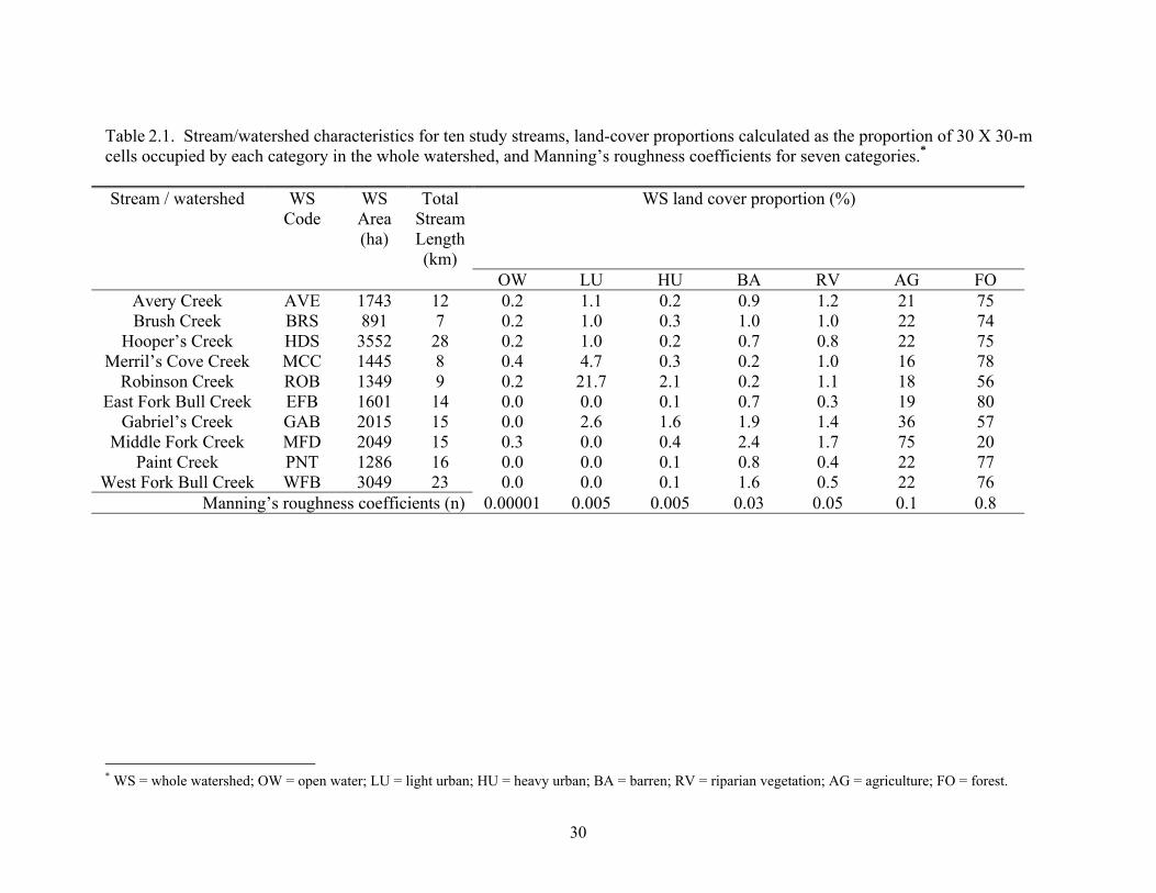
Table 2.1. Stream/watershed characteristics for ten study streams, land-cover proportions calculated as the proportion of 30 X 30-m cells occupied by each category in the whole watershed, and Manning’s roughness coefficients for seven categories.* Stream / watershed WS

Code WS Area (ha)

Total Stream Length (km)

WS land cover proportion (%)

OW LU HU BA RV AG FOAvery Creek AVE 1743 12 0.2 1.1 0.2 0.9 1.2 21 75Brush Creek

BRS 891 7 0.2 1.0 0.3 1.0 1.0 22 74Hooper’s Creek HDS 3552 28 0.2 1.0 0.2 0.7 0.8 22 75

Merril’s Cove Creek MCC 1445 8 0.4 4.7 0.3 0.2 1.0 16 78Robinson Creek ROB 1349 9 0.2 21.7 2.1 0.2 1.1 18 56

East Fork Bull Creek EFB 1601 14 0.0 0.0 0.1 0.7 0.3 19 80Gabriel’s Creek GAB 2015 15 0.0 2.6 1.6 1.9 1.4 36 57

Middle Fork Creek

MFD 2049 15 0.3 0.0 0.4 2.4 1.7 75 20Paint Creek PNT 1286 16 0.0 0.0 0.1 0.8 0.4 22 77

West Fork Bull Creek WFB 3049 23 0.0 0.0 0.1 1.6 0.5 22 76Manning’s roughness coefficients (n) 0.00001 0.005 0.005 0.03 0.05 0.1 0.8

* WS = whole watershed; OW = open water; LU = light urban; HU = heavy urban; BA = barren; RV = riparian vegetation; AG = agriculture; FO = forest.

30

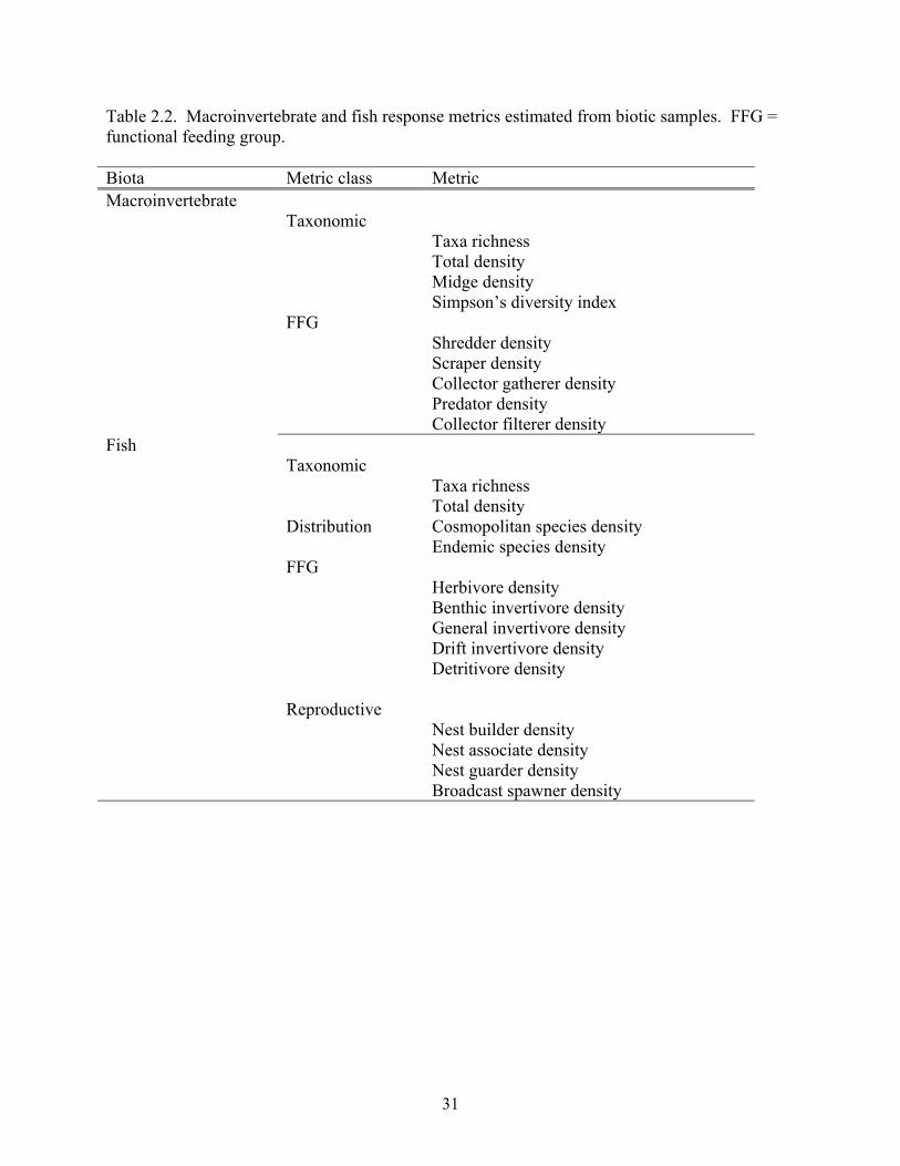
Table 2.2. Macroinvertebrate and fish response metrics estimated from biotic samples. FFG = functional feeding group. Biota Metric class Metric Macroinvertebrate Taxonomic Taxa richness Total density Midge density Simpson’s diversity index FFG Shredder density Scraper density Collector gatherer density Predator density Collector filterer density Fish Taxonomic Taxa richness Total density Distribution Cosmopolitan species density Endemic species density FFG Herbivore density Benthic invertivore density General invertivore density Drift invertivore density Detritivore density Reproductive Nest builder density Nest associate density Nest guarder density Broadcast spawner density

31

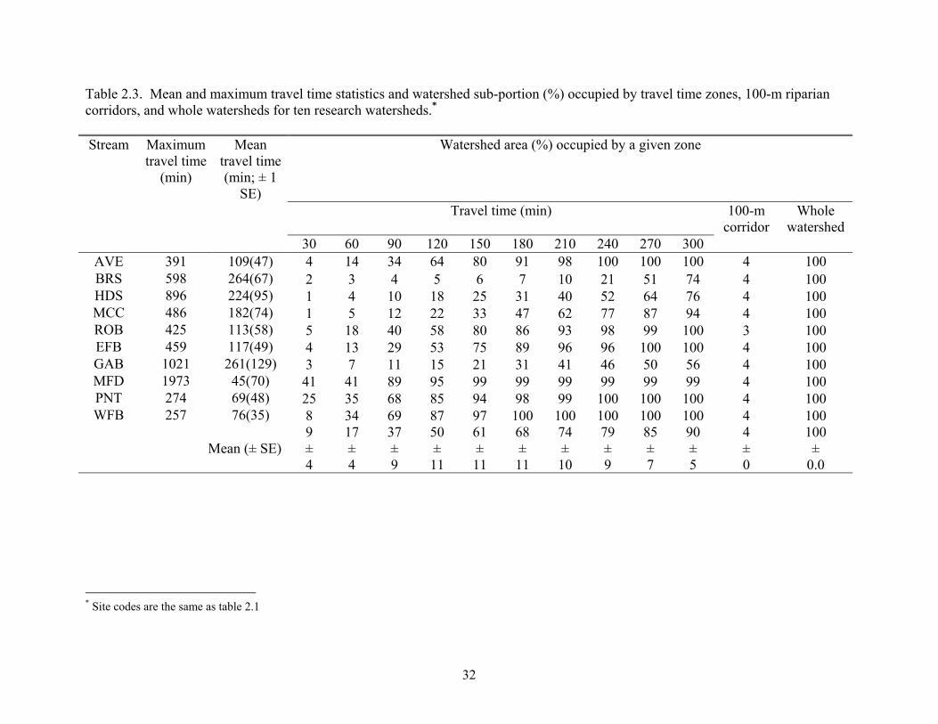
Table 2.3. Mean and maximum travel time statistics and watershed sub-portion (%) occupied by travel time zones, 100-m riparian corridors, and whole watersheds for ten research watersheds.* Stream Maximum

travel time (min)

Mean travel time (min; ± 1

SE)

Watershed area (%) occupied by a given zone

Travel time (min) 100-mcorridor

Whole watershed

30 60 90 120 150 180 210 240 270 300 AVE 391 109(47) 4 14 34 64 80 91 98 100 100 100 4 100BRS

598 264(67) 2 3 4 5 6 7 10 21 51 74 4 100HDS 896 224(95) 1 4 10 18 25 31 40 52 64 76 4 100MCC 486 182(74) 1 5 12 22 33 47 62 77 87 94 4 100ROB 425 113(58) 5 18 40 58 80 86 93 98 99 100 3 100EFB 459 117(49) 4 13 29 53 75 89 96 96 100 100 4 100GAB 1021 261(129) 3 7 11 15 21 31 41 46 50 56 4 100MFD 1973 45(70) 41 41 89 95 99 99 99 99 99 99 4 100PNT 274 69(48) 25

35 68 85 94 98 99 100 100 100 4 100

WFB 257 76(35) 8 34 69 87 97 100 100 100 100 100 4 100

Mean (± SE) 9 ± 4

17 ± 4

37 ± 9

50 ± 11

61 ± 11

68 ± 11

74 ± 10

79 ± 9

85 ± 7

90 ± 5

4 ± 0

100 ±

0.0

* Site codes are the same as table 2.1

32

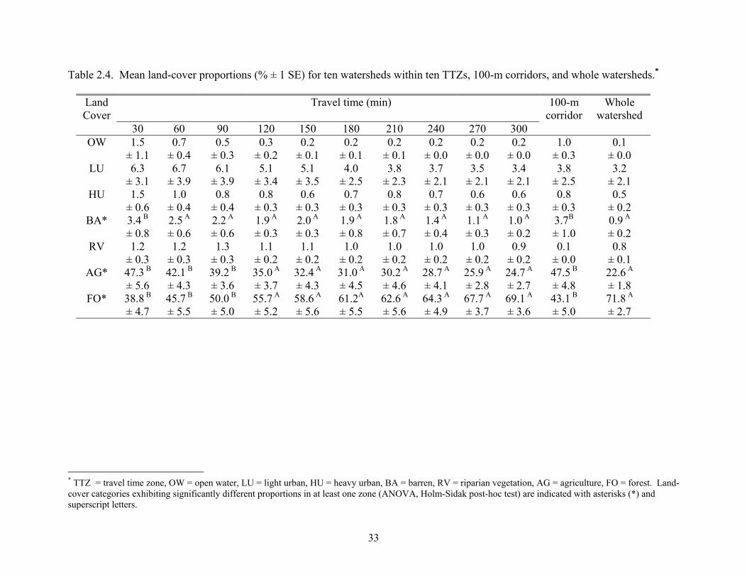
Table 2.4. Mean land-cover proportions (% ± 1 SE) for ten watersheds within ten TTZs, 100-m corridors, and whole watersheds.*

Land Cover

Travel time (min) 100-mcorridor

Whole watershed

30 60 90 120 150 180 210 240 270 300 OW

1.5

± 1.1 0.7

± 0.4 0.5

± 0.3 0.3

± 0.2 0.2

± 0.1 0.2

± 0.1 0.2

± 0.1 0.2

± 0.0 0.2

± 0.0 0.2

± 0.0 1.0

± 0.3 0.1

± 0.0 LU

6.3

± 3.1 6.7

± 3.9 6.1

± 3.9 5.1

± 3.4 5.1

± 3.5 4.0

± 2.5 3.8

± 2.3 3.7

± 2.1 3.5

± 2.1 3.4

± 2.1 3.8

± 2.5 3.2

± 2.1 HU

1.5

± 0.6 1.0

± 0.4 0.8

± 0.4 0.8

± 0.3 0.6

± 0.3 0.7

± 0.3 0.8

± 0.3 0.7

± 0.3 0.6

± 0.3 0.6

± 0.3 0.8

± 0.3 0.5

± 0.2 BA*

3.4 B

± 0.8 2.5 A

± 0.6 2.2 A

± 0.6 1.9 A

± 0.3 2.0 A

± 0.3 1.9 A

± 0.8 1.8 A

± 0.7 1.4 A

± 0.4 1.1 A

± 0.3 1.0 A

± 0.2 3.7B

± 1.0 0.9 A

± 0.2 RV

1.2

± 0.3 1.2

± 0.3 1.3

± 0.3 1.1

± 0.2 1.1

± 0.2 1.0

± 0.2 1.0

± 0.2 1.0

± 0.2 1.0

± 0.2 0.9

± 0.2 0.1

± 0.0 0.8

± 0.1 AG*

47.3 B

± 5.6 42.1 B

± 4.3 39.2 B

± 3.6 35.0 A

± 3.7 32.4 A

± 4.3 31.0 A

± 4.5 30.2 A

± 4.6 28.7 A

± 4.1 25.9 A

± 2.8 24.7 A

± 2.7 47.5 B

± 4.8 22.6 A

± 1.8 FO*

38.8 B

± 4.7 45.7 B

± 5.5 50.0 B

± 5.0 55.7 A

± 5.2 58.6 A

± 5.6 61.2A

± 5.5 62.6 A

± 5.6 64.3 A

± 4.9 67.7 A

± 3.7 69.1 A

± 3.6 43.1 B

± 5.0 71.8 A

± 2.7

* TTZ = travel time zone, OW = open water, LU = light urban, HU = heavy urban, BA = barren, RV = riparian vegetation, AG = agriculture, FO = forest. Land-cover categories exhibiting significantly different proportions in at least one zone (ANOVA, Holm-Sidak post-hoc test) are indicated with asterisks (*) and superscript letters.

33

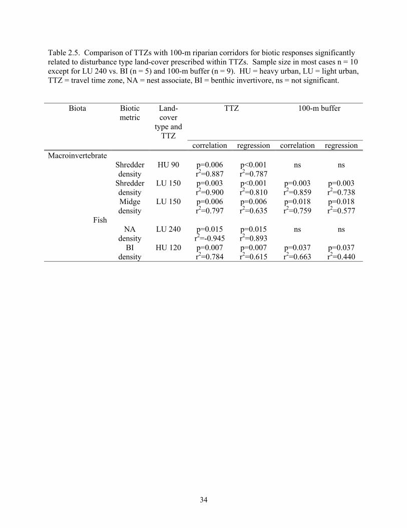
Table 2.5. Comparison of TTZs with 100-m riparian corridors for biotic responses significantly related to disturbance type land-cover prescribed within TTZs. Sample size in most cases n = 10 except for LU 240 vs. BI (n = 5) and 100-m buffer (n = 9). HU = heavy urban, LU = light urban, TTZ = travel time zone, NA = nest associate, BI = benthic invertivore, ns = not significant.

Biota Biotic metric

Land-cover

type and TTZ

TTZ 100-m buffer

correlation regression correlation regression Macroinvertebrate

Shredder density

HU 90 p=0.006 r2=0.887

p<0.001 r2=0.787

ns ns

Shredder density

LU 150 p=0.003 r2=0.900

p<0.001 r2=0.810

p=0.003 r2=0.859

p=0.003 r2=0.738

Midge density

LU 150 p=0.006 r2=0.797

p=0.006 r2=0.635

p=0.018 r2=0.759

p=0.018 r2=0.577

Fish NA

density LU 240 p=0.015

r2=-0.945 p=0.015 r2=0.893

ns ns

BI density

HU 120 p=0.007 r2=0.784

p=0.007 r2=0.615

p=0.037 r2=0.663

p=0.037 r2=0.440

34

C D

A B

Legend

Watershed Watershed hydrology

Rainfall Zone of influence

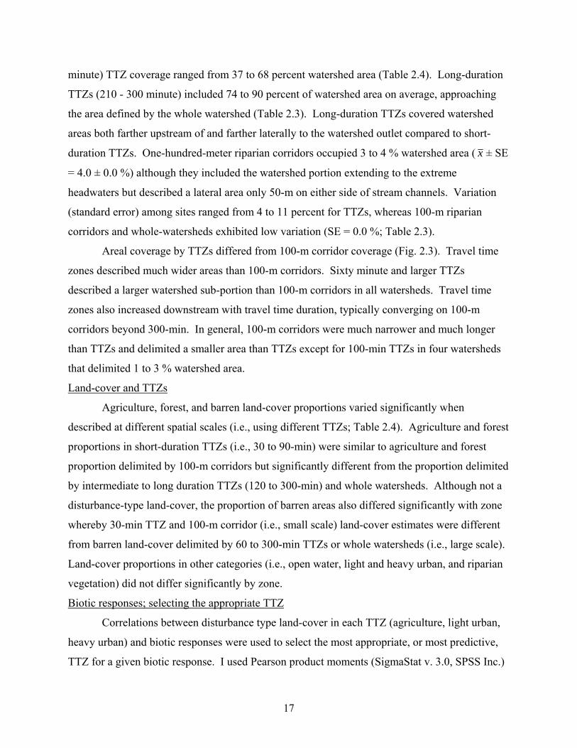
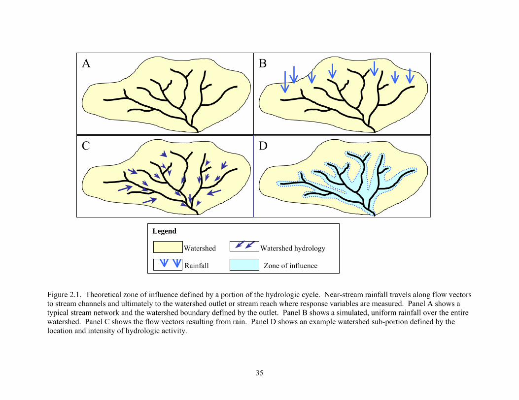
Figure 2.1. Theoretical zone of influence defined by a portion of the hydrologic cycle. Near-stream rainfall travels along flow vectors to stream channels and ultimately to the watershed outlet or stream reach where response variables are measured. Panel A shows a typical stream network and the watershed boundary defined by the outlet. Panel B shows a simulated, uniform rainfall over the entire watershed. Panel C shows the flow vectors resulting from rain. Panel D shows an example watershed sub-portion defined by the location and intensity of hydrologic activity.

35

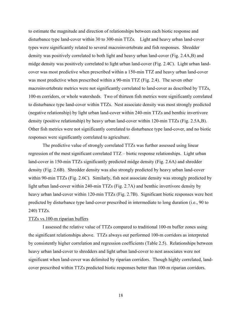
Travel Time (min)MCC stream

306090120180240Watershed boundary

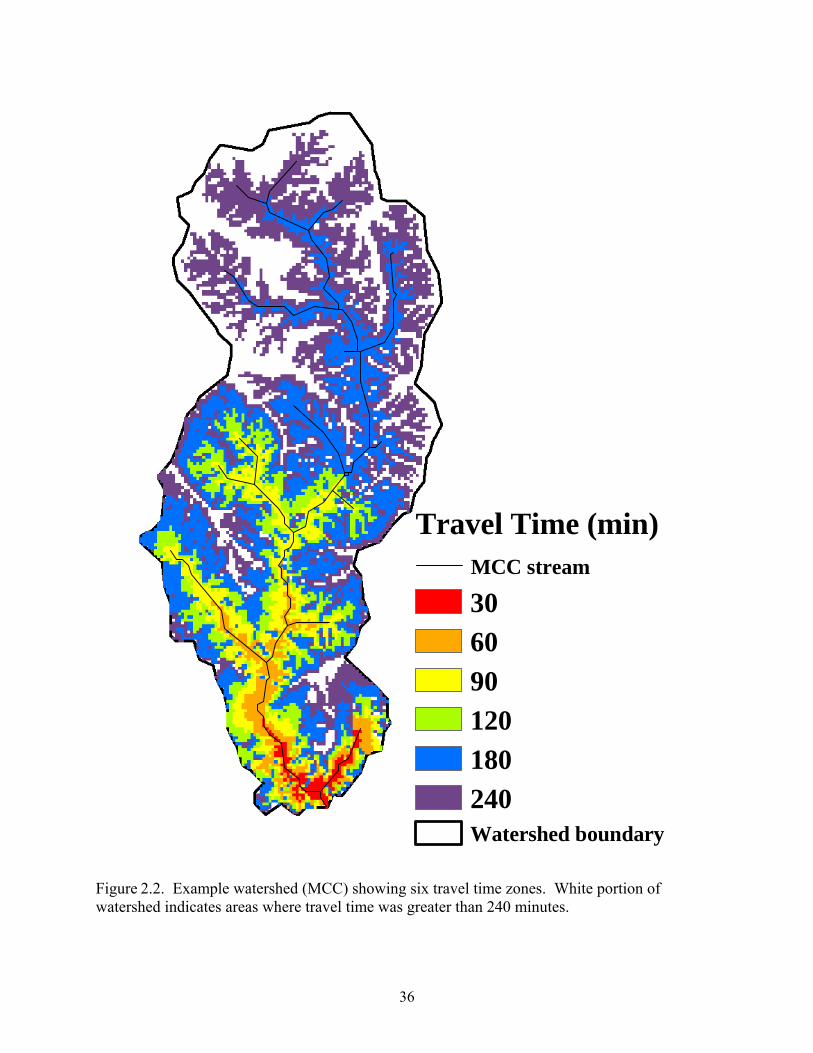
Figure 2.2. Example watershed (MCC) showing six travel time zones. White portion of watershed indicates areas where travel time was greater than 240 minutes.

36

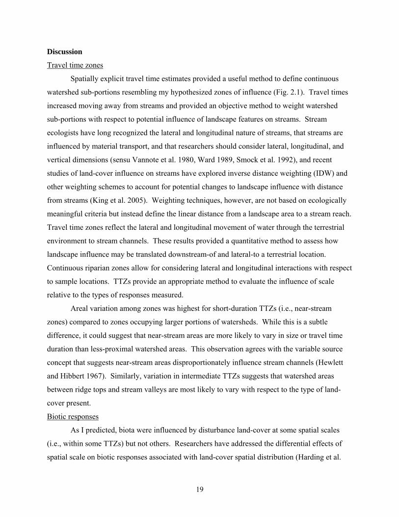
150 180120

60 9030

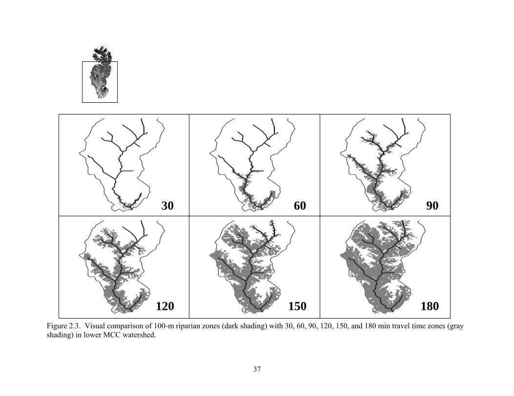
Figure 2.3. Visual comparison of 100-m riparian zones (dark shading) with 30, 60, 90, 120, 150, and 180 min travel time zones (gray shading) in lower MCC watershed.

37

Hea

vy u

rban

vs.

shre

dder

den

sity

-0.8

-0.4

0.0

0.4

0.8

1.2

Ligh

t urb

an v

s. sh

redd

er d

ensi

ty

0.2

0.4

0.6

0.8

1.0

TTZ0 60 120 180 240 300 360

Ligh

t urb

an v

s.m

idge

den

sity

0.0

0.4

0.8

A

B

C

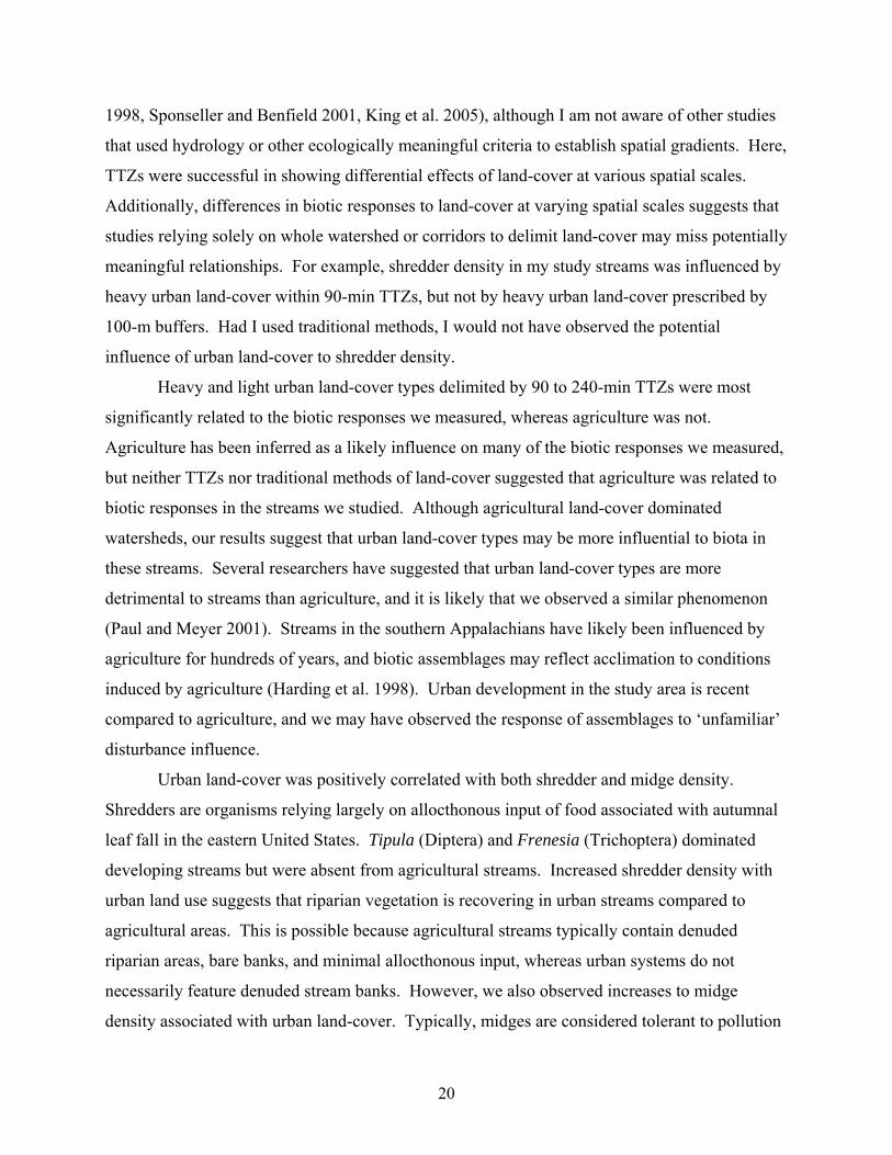
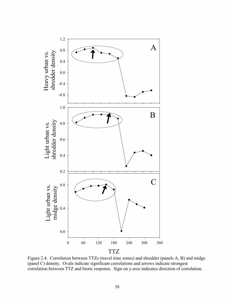
Figure 2.4. Correlation between TTZs (travel time zones) and shredder (panels A, B) and midge (panel C) density. Ovals indicate significant correlations and arrows indicate strongest correlation between TTZ and biotic response. Sign on y-axis indicates direction of correlation.

38

Ligh

t urb

an v

s. fis

h N

A

-0.9

-0.6

-0.3

TTZ0 60 120 180 240 300 360

Hea

vy u

rban

vs.

fish

BI

0.3

0.6

0.9

A

B

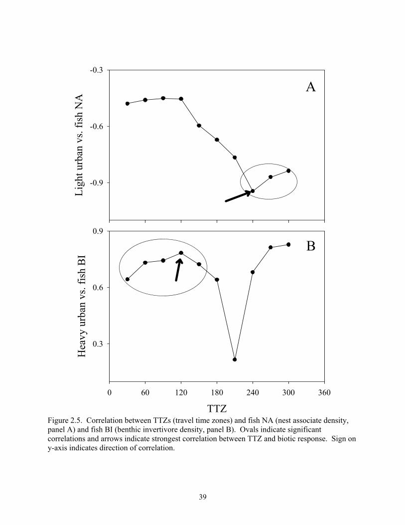
Figure 2.5. Correlation between TTZs (travel time zones) and fish NA (nest associate density, panel A) and fish BI (benthic invertivore density, panel B). Ovals indicate significant correlations and arrows indicate strongest correlation between TTZ and biotic response. Sign on y-axis indicates direction of correlation.

39

Light urban land cover (arcsine %) in 150-min TTZ0.0 0.1 0.2 0.3 0.4 0.5 0.6 0.7

Mid

ge d

ensi

ty (#

m-2

)

0

100

200

300

400

500

p = 0.006r2 = 0.635

Light urban land-cover (arcsine %) in 150-min TTZ0.0 0.1 0.2 0.3 0.4 0.5 0.6 0.7

Shre

dder

den

sity

(# m

-2)

0

25

50

75

p < 0.001r2 = 0.810

Heavy urban land cover (arcsine %) in 90-min TTZ0.00 0.05 0.10 0.15 0.20 0.25

Shre

dder

den

sity

(# m

-2)

-20

0

20

40

60

80

p < 0.001r2 = 0.787

A

B

C

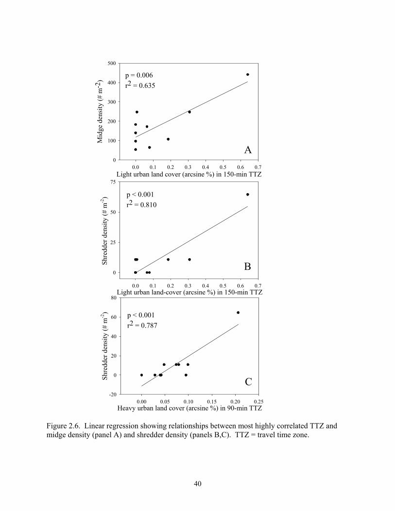
Figure 2.6. Linear regression showing relationships between most highly correlated TTZ and midge density (panel A) and shredder density (panels B,C). TTZ = travel time zone.

40

Light urban land cover (arcsine %) in 240-min TTZ0.0 0.1 0.2

Fish

NA

den

sity

(# m

-2)

-0.4

0.0

0.4

0.8

1.2

Heavy urban land cover (arcsine %) in 90-min TTZ0.00 0.05 0.10 0.15 0.20

Fish

BI d

ensi

ty (#

m-2

)

0.0

0.1

0.2

0.3

0.4

p = 0.015r2 = 0.893

p = 0.007r2 = 0.615

A

B

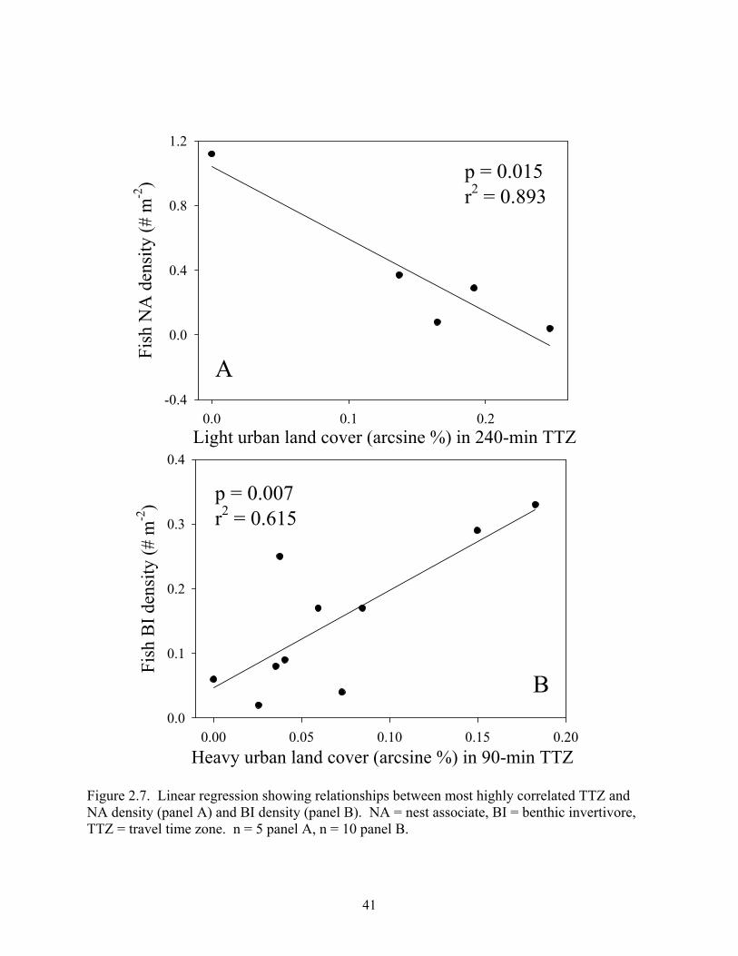
Figure 2.7. Linear regression showing relationships between most highly correlated TTZ and NA density (panel A) and BI density (panel B). NA = nest associate, BI = benthic invertivore, TTZ = travel time zone. n = 5 panel A, n = 10 panel B.

41

Chapter 3: Stream physical and biotic responses to rural development in historically agricultural watersheds

Abstract

I investigated whether rural development differentially influenced the physical and biotic

characteristics of historically agricultural streams. I quantified physical and biotic elements in

ten 3rd – 4th streams that drained historically agricultural watersheds located near Asheville, NC

in the southern Appalachians. Five watersheds contained recent rural development in areas

proximal to streams and five watersheds were not currently undergoing rural development. Five

hydrologic, ten geomorphic, six erosional, three depositional (i.e. substrate), thirteen fish, and

eight macroinvertebrate variables were estimated in the study streams. A total of 46 elements

were compared using t-tests and MANOVA to detect differential influence of rural development

and agricultural land-uses. Differences in land-cover influence were also assessed using

ordination to detect subtle differences in taxonomic composition and abundance. Storm flow

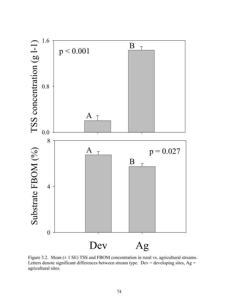
total suspended solid concentration (TSS) and substrate inorganic matter content were

significantly lower in streams influenced by rural development. This suggests that watershed

hydrology, sediment delivery, and sediment composition might be important factors influencing

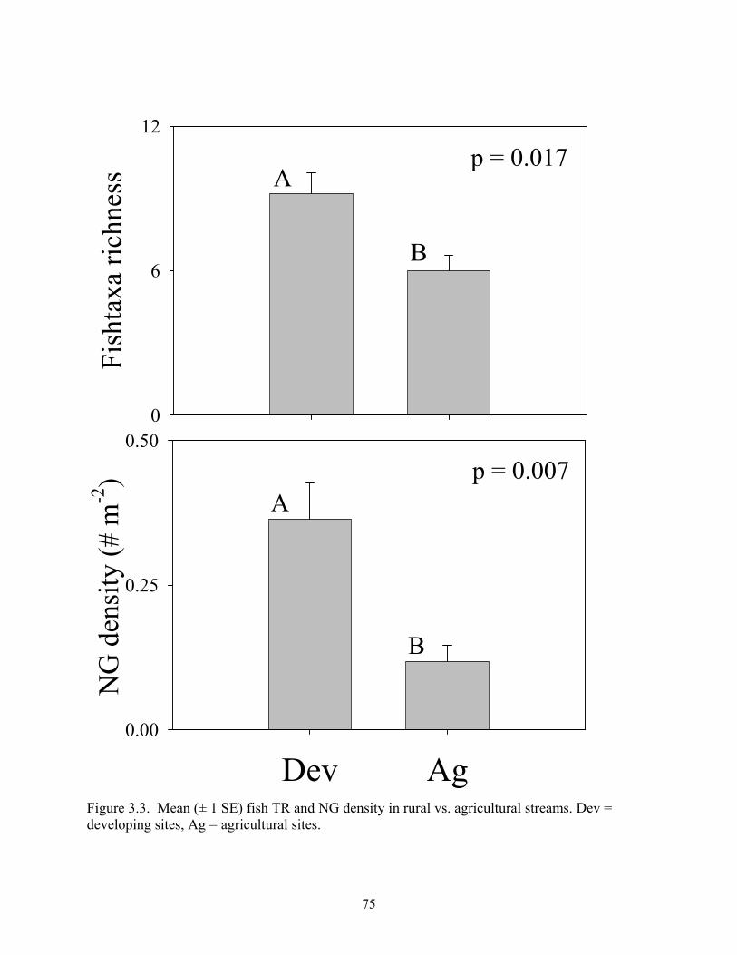
biota in streams draining agriculture versus rural development. Fish taxa richness and the

density of non-guarding fishes were significantly higher in rural development sites versus

agriculture sites. Though no significant differences in other fish or macroinvertebrate metrics

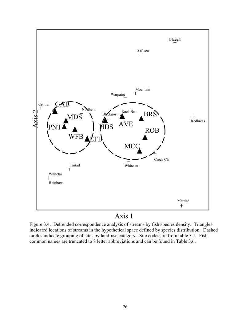
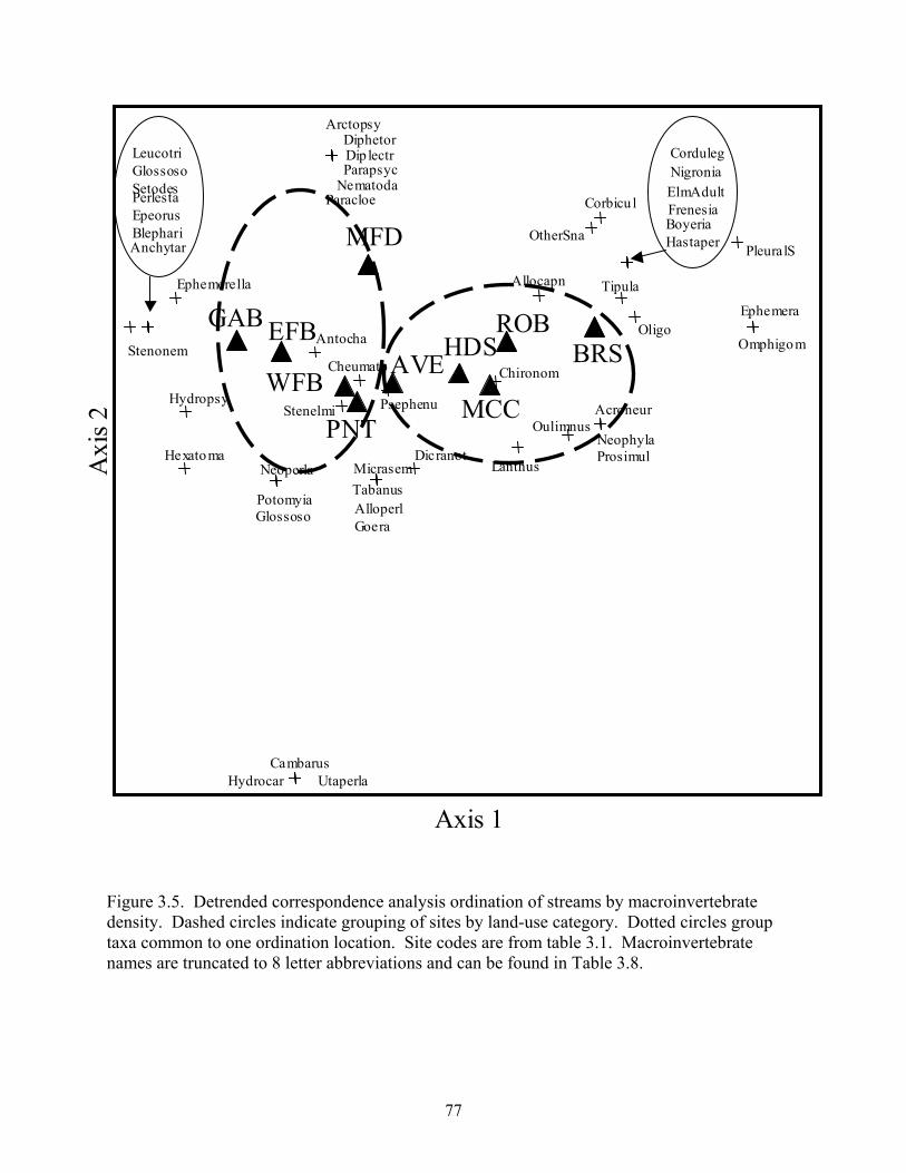
were detected, ordination of sites by fish and macroinvertebrate species abundance separated

stream types by land-use and suggested that biotic assemblages in developing streams were

distinct from those in agricultural streams and that some taxa may have been influenced by rural

development. My results suggest that assemblages were likely influenced by altered sediment

dynamics associated with rural development. Streams did not appear to be further impaired by

rural development, although assemblages were structurally different with stream type. I

conclude that the influence of rural development to historically agricultural southern

Appalachian streams is subtle but biotic assemblages in each stream type were different.

42

Introduction

Anthropogenic disturbance of the landscape is known to influence physical and biotic

elements of stream ecosystems. Influences of agricultural and urban activities, including nutrient

enrichment, tilling, animal grazing, chemical contamination, and building of human

infrastructure, have been studied intensively for the last thirty years (Heimlich and Anderson

2001, Paul and Meyer 2001). This research has identified how streams respond to anthropogenic

disturbance with respect to hydrologic (e.g., Poff and Allan 1995, Jones et al. 2000), geomorphic

(e.g., Rhoads and Cahill 1999, Stanley et al. 2002), sediment (Trimble 1997), and biotic (e.g.,

Harding et al. 1998, Wang et al. 2001, Sutherland et al. 2002) elements. Agriculture is known to

alter stream hydrology and geomorphology, reduce taxonomic diversity, and alter biotic structure

and function (Harding et al. 1998, Cuffney et al. 2000). Urban development as also been shown

to influence local hydrologic, geomorphic, and biotic stream elements (Wear et al. 1998, Paul

and Meyer 2001). Both land-use types are known to impair physical and biotic stream elements.

Individually, agriculture and urban development induce characteristic physical responses

in streams that can impair biota. Both disturbance types induce changes to hydrology and

geomorphology (Heimlich and Anderson 2001). Both can enhance erosion due to the removal of

rooted riparian vegetation (Neller 1988, Trimble 1997). In agricultural systems, erosional

dynamics alter the concentration of in-stream suspended sediments, especially during storms.

Removal of watershed vegetation also alters hydrologic activity in agricultural watersheds,

which often results in higher maximum flows and more dynamic sediment movement (Bhaduri

et al. 2000, Swank et al. 2001). Increased impervious surface cover (ISC) exacerbates overland

flow hydrology in urban systems, where overland flow often dominates stream hydrographs

(Jennings and Jarnagin 2002). Agricultural chemicals, including fertilizers and pesticides,

introduced to streams through runoff also result in biotic impairment.

Rural development is an increasingly common phenomenon of recent interest to

scientists, managers, and policy makers because it is a different form of urbanization that may

differ in its influence. Rural development occurs in metropolitan or urban areas associated with

urban sprawl, and includes the building of roads, parking lots, and housing developments.

Unlike urbanization, rural development is typically characterized as conserving a greater degree

of green space than true urban development (McDonnell and Pickett 1990, Heimlich and

Anderson 2001). I define rural development as being similar to low-intensity urbanization but

43

occurring in association with smaller cities (i.e., population < 250,000) that sprawl into

surrounding rural areas. Rural development could therefore induce a similar, but less severe,

influence as urban development.

The combination of agricultural and rural development disturbances to streams is an

increasingly common scenario associated with urban sprawl (Meyer and Turner 1992, Hunter

2000). The United Nations predicts that 85 - 90 percent of projected world population growth

between 2000 and 2030 will occur as urban sprawl (United Nations 1999). The coupling of

increased housing needs due to urban sprawl with the availability of formerly agricultural lands

leads to rural development for housing developments and urban structures (Ramankutty et al.

2002). The decline of small-scale agriculture due to competition with agribusiness has increased

the availability of agricultural lands to developers (Heimlich and Anderson 2001). In the

southeastern US, rural development likely differs from urban development in the intensity and

scope of the influence these disturbances have on the landscape.

I asked whether rural development altered physical and biotic characteristics of streams

historically impaired by agriculture. Studies of stream responses to urban land-cover suggest

that watershed hydrology can change dramatically relative to forested or un-urbanized systems

(Paul and Meyer 2001). I predicted that rural development might induce a similar effect, but at a

lower intensity. I expected rural development to induce flashier hydrographs and greater

variation in hydrologic activity. I also expected that geomorphology and erosion dynamics

would respond to increasing rural development relative to agricultural streams. I predicted that

developing streams would become more channelized (i.e., have deeper and narrower stream

channels) and potentially carry higher suspended sediment loads associated with erosion. I

expected substrata in developing streams to have a smaller mean size and contain a higher

amount of fine sediments relative to agricultural streams. I expected fish and macroinvertebrate

assemblages to differ with rural development in response to altered hydrology and erosion. I

predicted that biota sensitive to altered hydrology or sedimentation would be less abundant, or

absent from developing streams. Fish and macroinvertebrate assemblages were predicted to

show lower taxa richness and density, higher cosmopolitan fishes relative to endemics, and lower

diversity of trophic (fish and macroinvertebrates) and reproductive (fish) strategies. I

hypothesized that if rural development induced a measurable effect then streams would contain

44

different assemblages reflecting adaptation or acclimation of taxa to altered hydrology and

sediment dynamics.

Methods

Research watersheds

Streams in the southern Appalachians have been affected by agriculture since pre-

European settlement (SAMAB 1996). Several researchers investigating legacy effects of land-

cover in this area have documented this history and the condition of local streams (Harding et al.

1998, Wear and Bolstad 1998). In western North Carolina, rural development is occurring as the

city of Asheville sprawls into the surrounding, historically agricultural landscape.

I identified potential study areas in 3rd – 4th order streams draining watersheds featuring

agriculture and rural development. I verified the presence of agricultural and development

activity in watersheds near Asheville, visiting potential streams to observe watershed land-cover

(i.e., the presence of agriculture and rural development). I quantified land-cover using the 1993

USGS national land-cover database (NLCD), combining NLCD land-use categories to

agriculture, urban, forest, and other (USGS MRLC, draft, 2002; Homer et al. 2002). More recent

data were unavailable for the study area preventing quantifying more recent land-cover.

However, 1993 data largely verified visual estimates and provided approximations of land-cover

in the study area (Table 3.1).

Suitable development sites needed to have been influenced by legacy agriculture and

recent rural development located near an appropriately sized stream. These criteria proved

difficult to meet, largely because rural development was spatially patchy and often did not occur

in a portion of a watershed proximal to an appropriate-size stream. Often, rural development

was located either too far from a stream or in an area not known to have been influenced by

legacy agriculture. The five suitable watersheds meeting the criteria for rural development were

compared to five similar streams (with respect to geologic, edaphic, and elevational

characteristics) in the region that did not feature new developing areas (i.e., watersheds were

mostly agricultural; Figure 3.1). I was able to identify five streams in the French Broad River

basin that were historically impaired by agriculture but were currently (since at least 2000,

~2001) being developed to rural dwellings. Study watersheds ranged from 987 to 3552 ha ( x =

1908 ± 257 ha; Table 3.1).

45

In addition to land-cover constraints, watersheds were selected for similar geology, soil

composition, stream network development, drainage area, and gradient using GIS. Every effort

was made to ensure that the major difference among ten streams was the presence or absence of

rural development proximal to stream channels. Controlling for these effects allowed us to

attribute differences, with strong likelihood, to land-cover effects. To determine whether streams

in historically agricultural watersheds were affected by rural development, I measured stream

elements that have been shown to respond to agriculture and/or urbanization. Elements were

quantified within 3rd – 4th order 100-m stream reaches defining the downstream watershed

terminus.

Physical elements

Hydrologic features

Stream stage height was identified using a TopCon® laser survey unit to establish a

permanent zero height of baseflow (0-cm). Discharge was measured and stage height recorded

approximately monthly for 32 months at various flows. Rating curves estimating the relationship

between stage height and discharge were developed to estimate discharge beyond the measurable

range. Baseflow discharge (stage = 0-cm), storm flow discharge (stage = 50-cm), and the slope

of the discharge / stage rating curve (an indication of flashiness) were estimated from these data.

The difference in magnitude between baseflow and storm flow (Qdiff) was used as a measure of

flashiness or how quickly streamflow responded to precipitation.

Watershed travel time for rainfall was estimated using Hydrologic Engineering Center –

Hydrologic Modeling System (HEC-HMS) equations (See Chapter 2, this dissertation; USACE

2000). Estimates of surface roughness, hillslope gradient, and proximity to stream channels were

used to calculate the time required for rainfall to travel between the terrestrial environment and

the watershed outlet. We expected surface hydrology to be important to these streams affected

by ISC and travel time estimates were used to quantify differences in land-cover factors (i.e.,

presence or absence of rural development). Mean and maximum travel times were calculated for

each watershed and compared by land-use type.

Geomorphic features

Three channel cross-sections were measured (TopCon®) along each 100-m reach

periodically in 2002 and 2003 to estimate changes to channel morphology. Eleven metrics were

derived from these cross-sections (Montgomery and MacDonald 2002). Bank height, the

46

elevation difference between maximum thalweg depth and floodplain height, was calculated for

each stream bank and averaged as a measure of channel deepening or incision magnitude. Bank

incision ratio, the proportionate angles between maximum thalweg depth and floodplain height,

was calculated for each bank. Both bank height and incision ratio were measured once during

each sample year and the difference was calculated to estimate stream channel movement

between sample dates.

I also calculated average baseflow width and depth and the mean width / depth ratio for

each stream reach. Hydrologic and geomorphic information was used to calculate the Froude (Fr

= V / squareroot(g*D)) number, where V is the mean water velocity (m s-1), D is the mean

baseflow depth (m), and g is the gravitational constant (m s-2; from Gordon et al. 2004).

Erosional features

Ten erosional metrics were estimated by measuring both suspended sediment

concentration and bedload composition. Suspended sediments were collected using rising-limb

sediment samplers (Braatz 1961) that collected stream sediment / water samples on the rising-

limb of storm hydrographs. Bottles were collected after streams returned to baseflow and

analyzed for total-suspended solids (TSS) and percent fine particulate organic matter (FPOM)

using the ash-free-dry-mass (AFDM) method (Eaton et al. 1995). Ash-free-dry-mass was used

to estimate the proportion of inorganic and organic content by filtering a known volume of

stream water, drying and ashing the filtered sample, and calculating the dry and ash weights.

The weight per volume of ashed material was used to approximate the concentration of inorganic

sediments, and the difference between ash weight and dry weight to approximate the organic

content. Similarly, bedload samples were collected using 50-cm long, 12-cm diameter PVC

tubes buried within channels in the stream substrate. These containers passively collected

bedload during intervals ranging from 0.5 to 1 month. Bedload samples were stored in 12 l

containers, from which a subsample of fine benthic organic matter (FBOM; 0.45-µm < FBOM <

1-mm) was removed from a slurry to estimate organic and inorganic matter content of bedload

by the AFDM method. The remaining bedload sample was then dried and sieved to calculate

D50 and percent fine substrates (< 0.5-mm).

Depositional features

Benthic substrate characteristics were estimated from three samples collected once at a

riffle-pool interface downstream of a typical riffle in each stream. Samples were collected with a

47

spade, placed into a bucket, air dried, and dry sieved. This method only effectively sampled

substrate smaller than 10-cm and likely underestimated the contribution of fine substrates

because some material was lost during collection (Bunte and Abt 2001). However, I assumed

the loss of fine substrate (e.g., sand) associated with the sample method would be similar among

all streams. Similar to bedload sampling, wet substrate samples were slurried to collect a

subsample for AFDM to estimate organic matter content in fine sediments.

Biotic assemblages

Fishes were sampled during August in 2002 and 2003 using single pass backpack

electrofishing along 100-m stream reaches. Reaches were subdivided into 1 to 10-m sections

using natural breaks in habitat units as boundaries between sub-units. A block seine (5-mm

mesh) was established at the downstream end of each sub-unit and electrofishing helped herd

fishes into the seine. Fishes were collected and identified to species after each sub-unit was

sampled and returned downstream. Density was estimated as the number of individuals collected

per stream area sampled (100-m X average stream width; # m-2). No differences were detected

in density or species composition between the annual samples and only 2002 data were

considered in further analyses.

Fishes were assigned to distributional, reproductive, and trophic guilds based on available

information for each species. Distribution status reflects historic occurrence of a species within

and across drainages (Scott and Helfman 2001). Cosmopolitan species are widely distributed

through a drainage and span stream order and habitat gradients. Endemic species are localized,

are often only found in a small portion of a drainage often in a very localized area. Endemic

fishes have been associated with highland areas, or higher gradient, lower-order streams (Scott

and Helfman 2001). Scott and Helfman (2001) showed that two distinct fish assemblages often

occur in southern Appalachain streams reflecting high or low endemism.

Fishes were assigned to reproductive guilds based on recorded spawning habits of each

species. Fishes vary in their mode of reproduction and can build nests, guard eggs, or simply

broadcast eggs across the benthos. We placed each species encountered into 1 of 5 reproductive

guilds (Jenkins and Burkhead 1994, Etnier and Starnes 1993). Nest builders (NB) are fishes that

build and guard nests and included centrarchids and the fantail darter. Nest associates (NA) are

fishes that often spawn in association with pebble mounds organized by another species and

included Whitetail shiner, Warpaint shiner, and Central stoneroller minnows. Burying non-

48

guarders (NG) are fishes that hide eggs in substrate without further parental care and included

species from several families. Broadcast spawners included species that spread eggs and milt

over an area of substrate without burying or providing parental care and included Blacknose dace

and White suckers.

Fish feeding habits were also used to categorize species by feeding strategy based on

recorded knowledge of each species (Jenkins and Burkhead 1994, Etnier and guild 1993).

Herbivores feed primarily on living plant material, algae, and detritus and included Bluegill,

Redbreast sunfish, Whitetail shiner and Blacknose dace. Invertivores eat insects and crustaceans

and were subdivided by the portion of the water column in which prey items are typically taken.

Benthic invertivores pick prey items from substrata and often have specialized subterminal

mouths designed for bottom feeding and included the Northern hogsucker. Drift invertivores lie-

and-wait for drifting prey to be delivered to them, and included Warpaint and Saffron shiners.

General invertivores are species known to collect prey items from multiple locations within a

stream and included Creek chub, Central stoneroller, Rock bass, and Rainbow trout. Last,

detritivores are species known to feed primarily on detritus and associated small organisms sifted

from decaying organic matter and included White sucker and Mountain brook lamprey.

Macroinvertebrates were collected during late April 2003 using twenty quantitative

(Surber, 500 µm mesh, 0.09 m2, 1.8 m2 total area sampled per 100-m reach). Density (# m-2) was

estimated from individual samples and average density by taxa calculated for each stream.

Macroinvertebrates were preserved in 80% ethanol and identified to the lowest possible

taxonomic level (typically genus). Taxa were placed into functional feeding groups (FFG) based

on the classification by Merrit and Cummins (1996) or expert opinion for macroinvertebrates in

southern Appalachian streams. Functional feeding groups included collector-filterers and

collector-gatherers known to remove particulate matter from the water column, shredders that

feed on decaying leaves, scrapers that have specialized mouthparts for removing algae from rock

surfaces, and predators that consume other animals. I did not consider ontogenetic changes in

feeding habits associated with early instars and assumed that individuals of a species could be

classified into a single FFG.

Statistics

In total I measured or estimated five hydrologic, ten geomorphic, six erosional, three

depositional (i.e., substrate) elements, thirteen fish, and eight macroinvertebrate metrics in each

49

stream (forty-six variables total). To detect differences attributable to rural development, each of

the sample means were compared using simple t-tests between five agriculture and five rural

development streams. Bonferroni adjustment was not necessary because the dependent variable

was different for each comparison (e.g., baseflow discharge, particle size, macroinvertebrate taxa

richness). I also used multivariate analysis of variance (MANOVA) to detect differences

associated with organizational levels (e.g., hydrology). This technique allowed consideration of

collinearity among intra-elemental variables (e.g., rating curve slope, mean travel time, etc.) that

were present within each variable category. MANOVA was used because the technique can

detect the influence of land-cover type on hydrology, geomorphology, erosional dynamics,

substrate composition, biotic metrics, or some combination.

I predicted that rural development might induce a similar but less intense influence to

streams than might urban development. To detect small differences in abiotic and biotic

responses that might not be apparent with t-tests, I used Detrended Correspondence Analysis

(DCA) to project sites in the space determined by abiotic or biotic characteristics (PCOrd v. 3.18,

MJM software, Oregon, USA). DCA considers sites and taxa, projecting each into the space

determined by weighted averages of taxa and site scores (Eigenvalues) along one or more axes.

Results

Physical responses

Hydrology

Hydrologic responses were not shown to be significantly different between stream type

with either t-tests or MANOVA (Table 3.2). Mean baseflow discharge was 40 ± 10 L s-1 in

developing streams and 36 ± 6 L s-1 in agricultural streams. Mean storm flow discharge (stream

flow occurring at stage = 50 cm) estimated from rating curves was 1208 ± 238 L s-1in

developing streams, and 2163 ± 1098 L s-1in agricultural streams. Rating curve slope averaged

0.9 ± 0.1 in streams draining both land use types. Mean watershed travel time was 178 ± 30 min

in developing streams, and 113 ± 39 min in agricultural streams. Mean maximum travel time

varied from 559 ± 91 min and 797 ± 325 min in developing and agricultural streams,

respectively.

The difference between baseflow and storm flow (Qdiff) averaged 1167 ± 240 L s-1in

developing streams, and 2123 ± 1094 L s-1in agricultural streams. This difference represents a

discharge increase of 1 to 2 orders of magnitude for streams that averaged 40 L s-1during typical

50

baseflow condition. Generally, all study streams appeared extremely flashy (C.L. Burcher,

personal observation), which was supported by USGS stream gauges located on the mainstem

Ivy River and near the confluence of Cane Creek on the mainstem French Broad River*. I did

not detect a difference in flashiness with stream type. Although I did not quantify flood

recurrence interval, and have no historic record documenting floods in these streams, I observed

several storms during the study period that would be considered catastrophic (i.e., streams

breached 100 yr floodplain stage multiple times during a single year), and stormflow recorded by

nearby USGS gauges during this period (March and April 2002 and 2003) were exceptionally

high. Stream channels had likely been previously influenced by such flows, and further

geomorphic changes would probably be induced only by extremely catastrophic flows beyond

these observed during the study (Paul and Meyer 2001).

Ordination (DCA) of sites by hydrologic variables indicated that Paint and Middle Fork

Creeks were outliers, separate from other streams and that these sites may be different with

respect the combined influence of the hydrologic variables I measured (Table 3.2).

Geomorphology

No significant geomorphic differences were detected between stream types using t-test or

MANOVA (Table 3.3). Bank height and incision ratio varied little between two sample years,

averaging 1.3 ± 0.0 m in year one for both stream types and 1.3 ± 0.0 m (dev) and 1.4 ± 0.1m

(ag) in year two. Bank height changed little between sample years and was 0.1 ± 0.0 in

developing streams and 0.2 ± 0.1 m in agricultural streams. Similarly, bank incision ratio

averaged 33 % in developing streams during both years and averaged 30 % (year 1) and 34 %

(year 2) in agricultural streams. Incision ratio changed an average of 2 ± 1 % in developing

streams and an average of 5 ± 3 % in agricultural streams between sample years. Mean baseflow

width was 3.7 ± 0.6 m in developing streams and 4.5 ± 0.3 m in agricultural streams. Mean

baseflow depth was 0.14 ± 0.02 m in developing streams and 0.19 ± 0.02 m in agricultural

streams. Mean width to depth ratio was 32 ± 9 in developing streams and 26 ± 4 in agricultural

streams. The average Froude number was 0.14 ± 0.02 and 0.11 ± 0.02 in developing and

agricultural streams, respectively, indicating that all streams were well below the threshold of

critical flow.

* http://waterdata.usgs.gov/nwis/rt

51

When sites were arranged in geomorphic space, DCA ordination indicated that Robinson

Creek (developing) and Brush Creek (agriculture) were separate from other streams but that no

land-cover influence was apparent. Separation of these two sites was related to the width / depth

ratios. This could be due to Robinson Creek being exceptionally wide and shallow, whereas

Brush Creek was narrow and deep (Table 3.3). Other sites clustered together intermediate to

Brush and Robinson creeks, and no land-cover influence was apparent.

Erosional sediment

Storm flow TSS concentrations were estimated from TSS rating curves (relating

discharge to TSS concentration) generated for four developing and two agriculture sites (Table

3.4). Storm flow TSS was not estimated for other streams due to lack of storm TSS samples.

Storm flow TSS concentration differed significantly between land-cover types (t-tests p < 0.001),

averaging 0.20 ± 0.10 g l-1 in developing streams and 1.4 ± 0.0 g l-1 in agricultural streams (Fig.

3.2A). However, percent organic matter ( x dev = 12 ± 3 %; x ag = 24 ± 11 %) of suspended

solids did not differ between stream types (Table 3.4).

Bedload characteristics were also similar between stream types and showed no significant

land-cover effect (Table 3.4). Bedload D50 averaged 2.9 ± 0.4 mm in developing streams and 2.2

± 0.9 mm in agricultural streams. Bedload mean percent fines averaged 32 ± 4 % in developing

streams and 36 ± 2 % in agricultural streams. Bedload % organic matter was similar in each

stream type and averaged 17 ± 1 % in developing stream and 13 ± 1 % in agricultural streams.

Ordination of erosional metrics indicated that East and West Fork Bull Creeks

(agriculture) and Brush Creek (developing) were separate from a group of the seven other

streams. However, this separation was likely influenced by zero values and reduced sample size

associated with sampler loss or inadequate replication of erosional characteristics (Table 3.4).

No land-cover influence associated with geomorphic attributes was apparent with DCA.

Depositional substrate

Depositional metrics were similar in streams draining different land-use types. However,

substrate organic matter content (FBOM) was significantly higher in developing sites (p < 0.05),

averaging 6.8 ± 0.3 % (vs. 5.8 ± 0.2 % in agricultural sites; Fig. 3.2B). Substrate D50 was

similar, averaging 14.7 ± 3.5 mm in developing sites and 17.0 ± 3.1 in developing sites (Table

3.5). Percent fine substrate was also similar among stream types, averaging 13.7 ± 4.4 % in

52

developing sites and 14.2 ± 4.3 % in agricultural sites. Ordination of sites by substrate attributes

did not indicate grouping structure or a land-use effect.

Biotic assemblages

Fifteen fish species were collected from streams and Robinson Creek (developing site)

contained the highest taxa richness in any single stream (11 species, Table 3.6). Developing

streams were dominated by Creek chub and Central stoneroller whereas Blacknose dace and

Fantail darter were dominant in agricultural streams. Whitetail shiner and rainbow trout were

absent from developing stream whereas agricultural streams did not contain Mottled sculpin,

Mountain brook lamprey, Rock bass, Saffron shiners, or Redbreast sunfish. Fish taxa richness

was significantly (p = 0.017) higher in developing sites, averaging 9 ± 0.9 taxa as opposed to

agricultural stream fish taxa richness, which averaged 6 ± 0.6 taxa (Fig. 3.3A). Non-guarding

fish density was also significantly (p = 0.007) higher in developing streams (Fig. 3.3B). In

general, fish assemblage metrics were similar among streams draining the two stream types.

Average total fish density was not different between stream types, and averaged 0.9 ± 0.2 in

developing streams and 1.3 ± 0.3 in agricultural streams (Table 3.7). No other differences were

detected in fish assemblages between stream types using t-tests. However, cosmopolitan fishes

numerically dominated in both stream types. Stream trophic structure was dominated by

herbivores and reproductive structure by either non-guarders (Fig. 3.3B) or nest associates (Table

3.7).

Despite general lack of significant differences between stream types suggested by

inferential statistics, ordination of sites in fish species space suggested that assemblages differed

with stream type. The arrangement of sites by species composition using DCA suggested

separation of sites based on fish taxa and further explained the variation behind this separation as

being a result of distinct assemblage composition in each stream type (Fig. 3.4). Axis 1

represented a gradient of species density and was largely driven by species absent in one land-

use type (e.g., Redbreast sunfish present only in developing streams). Little variation existed in

axis 2 (Eigenvalue 0.04): axis 1 having a much higher Eigenvalue (0.5). This suggests that most

of the variation in assemblage structure can be explained by the occurrence and relative density

of each taxa. Further, DCA distinguished between stream types based on fish assemblage

structure. Detrended correspondence analysis suggested that developing stream assemblages

were dominated by cyprinids including Warpaint shiners, Blacknose dace, Saffron shiners,

53

Central stonerollers, centrarchids including Bluegill, Redbreast sunfish, and Rock bass, and

Mountain brook lamprey (Fig. 3.4). Separation of agricultural streams by ordination was largely

driven by assemblages in these streams being dominated by Northern hogsuckers, Fantail darters,

and Whitetail shiners.

Macroinvertebrate assemblages in developing streams were dominated by dipterans and

largely by chironomids (Table 3.8). Agricultural streams also contained high midge density, but

were dominated by ephemeropterans of the genera Ephemerella, Stenonema, and Epeorus (Table

3.8). Nine taxa co-occurred in both stream types, most notably Chironomidae, pleurocerid

snails, ephemerellid mayflies, Psephenus and Stenelmis beetles, tipulid flies, and hydropsychid

caddisflies. Despite these similarities streams contained many taxa that only occurred in one

stream type.

None of the macroinvertebrate metrics I estimated differed significantly between stream

types (Table 3.9). Mean taxa richness was 11 ± 2 for all streams. Average total

macroinvertebrate density was 700 ± 199 in developing streams and 654 ± 202 in agricultural

streams. Midges comprised between 19 (agriculture) and 33 (developing) % of invertebrates by

density (dev x = 230 ± 57 m-2; ag x = 121 ± 35 m-2). Shredders were nearly absent from

agricultural streams ( x = 2 ± 2 m-2) but averaged 19 ± 11 m-2 in developing streams.

Macroinvertebrate assemblages in both stream types were dominated scraper or collector-

gatherering genera. Scrapers (dev x = 205 ± 60 m-2; ag x = 151 ± 82 m-2) comprised 29 % of

developing stream and 23% of agricultural stream assemblages. Collector gatherers (dev x =

138 ± 59 m-2; ag x = 245 ± 89 m-2) comprised 20 and 37% of developing and agricultural

streams assemblages, respectively. The average density of collector-filters was 60 ± 22 m-2 in

developing streams and 121 ± 25 m-2 in agricultural streams, and did not differ significantly

between the two land-uses. Predators comprised 7% of assemblages in developing streams ( x =

47 ± 17 m-2) and only 2% in agricultural streams ( x = 15 ± 8 m-2).

Detrended correspondence analysis by macroinvertebrate taxa indicated near separation

of streams by stream type (Fig. 3.5). The distribution of sites along axis 1 (Eigenvalue 0.48)

indicated two distinct macroinvertebrate groups that were separated by taxa present in only one

stream type. Axes 2 and 3 did not add explanatory value to axis 1 and were not interpreted.

54

Discussion

Physical responses

Total suspended solid concentration was significantly lower (p < 0.001) in streams

influenced by rural development than streams draining predominantly agricultural land-use

(Figure 2A). Although I initially expected TSS to increase with rural development, I attribute

this difference to altered overland flow and channel hydrology in developing streams.

Finkenbine et al. (2000) suggested that initially, urbanizing watersheds contribute more

suspended sediments associated with construction to streamflow, but during the second phase of

urbanization, suspended sediment loads decrease relative to pre-disturbance conditions. Lower

TSS concentration in developing streams could be because study streams were no longer

receiving sediments associated with the initial phases of construction. However, this would

imply that some hydrologic element interacted with sediments, and I did not detect an effect of

rural development on the hydrologic elements quantified in these study streams. It is possible

that some unmeasured hydrologic effect could have been influencing TSS in the streams I

studied, for example, streambed shear stress (Krishnappan 2004) or terrestrial erosion. Surface

runoff in agricultural areas may have been more erosional, delivering more suspended material to

river channels compared to runoff associated with rural development. Similarly, it is possible

that runoff in developed areas was exposed to a smaller volume of soil than agricultural runoff.

This is a plausible explanation because rural development features more impervious surface

cover, which has been shown to reduce the erosional potential of land surfaces (Jennings and

Jarnagin 2002). Many researchers have attributed lower suspended particulates to increased

impervious surface cover (Booth 1990, Crosbie and Chow-Frasier 1999). Similarly, in-stream

sediment re-suspension is known to contribute to total suspended solid concentration, and it is

uncertain whether higher TSS was due to near-stream erosion, in-stream re-suspension, or bank

failure (Owens and Walling 2002). It is likely that developing streams carried a reduced

suspended sediment load as a result of lower watershed terrestrial erosion due to the combination

of more ISC, and lower in-stream particulate re-suspension.

Substrate organic matter standing stocks (% FBOM) were significantly higher in streams

influenced by rural development (Fig. 2B). This suggests that the inorganic matter (IM)

proportion of substrata was lower with rural development, and is of particular interest

considering that total suspended solids were also lower in developing streams. Coupling TSS

55

and IM information suggests that agricultural streams were both more erosional in the terrestrial

environment (as indicated by higher TSS), and hydrologically more disturbing to the substrate.

Conversely, streams draining rural development had lower suspended sediments, yet FBOM

concentrations were higher relative to agricultural streams. It is possible that retention

mechanisms differed with land-cover type, though I did not quantify these features (Wang et al.

2001). Ultimately, these observations suggest that hydrology was different in the presence of

rural development, yet I did not observe differences in the hydrologic elements I measured.

However, the lack of significant differences in hydrologic elements may have been a result of

high variance associated with these measures, and the difficulties in quantifying them (see Table

2). It is possible that my measurement of hydrology was inadequate to capture differences in

hydrologic dynamics associated with land-use types. Hydrologic elements are notoriously

difficult to quantify due to the stochastic nature of storms (Wondzell and Swanson 1999, Lake

2000), variability between high-flow periods (Resh et al 1988), and long-term hydrologic

patterns (Richter et al. 1992).

Biotic responses

Ordination of streams by density of fish and macroinvertebrate taxa suggested that

distinct assemblages were present in each stream type (Figs. 3.4, 3.5). In each scenario, sites

separated (or nearly so) into two groups representing developing or agricultural streams.

Ordination clearly indicated unique assemblages with land-use type, and I attribute this

separation to altered hydrology and sediment dynamics. Alternatively, the nested condition of

sites within parent watersheds (e.g., agricultural sites all drain into Ivy Creek, developing sites all

located near Cane Creek) could explain differences in taxonomic composition. However,

mainstem streams were located in close proximity (~25 km), were joined by the French Broad

River, and would likely not inhibit fish movement between drainages. Similarly, watersheds

were within 25 km of each other and limited macroinvertebrate dispersal could not explain the

differences in macroinvertebrate assemblage composition we observed. If we assume the

likelihood of a taxa being present was similar for each stream type, the presence of rural

development near streams is a strong explanation of observed taxonomic differences.

Fish assemblages

Combination of ordination information and reproductive ecology of taxa helps explain

differences in fish assemblage structure with stream type. Developing streams contained

56

Redbreast, Bluegill, and Rock bass sunfishes whereas centrarchids were absent from agricultural

streams. Mottled sculpin was absent from agricultural streams, but occurred in 4 of 5 developing

streams. Higher density of non-guarding fishes in developing streams likely resulted from the

ability of centrarchids and sculpin to clean substrata for nests or tolerance to the hydrologic

regime present in developing streams. Higher inorganic sediments associated with agricultural

substrata could explain the reduced representation of nest builders in these streams. Nest

associates that were largely comprised of Central stoneroller and Whitetail shiner (Cyprinidae)

dominated agricultural streams. These two species typically spawn in association with aggregate

nest builders (e.g., Creek chub) but can spawn successfully in the absence of nests (Jenkins and

Burkhead 1994). The only nest-builders encountered in agricultural streams were Bluegill and

the percid Fantail darter and I assumed that cyprinid nest associates were spawning via

alternative methods in agricultural streams (Etneir and Starnes 1996).

Fish distribution status also helps explain site separation with ordination. Three fish

species endemic to highland streams, Warpaint and Saffron shiners and Mottled sculpin, were

collected in this study. Only Warpaint shiners were collected in agricultural streams, and the

reduced representation of endemic species could reflect higher relative ability of diverse habitat

and trophic resources in developing streams. Sculpin rely on benthic interstices for feeding and

reproduction and their absence from agricultural streams could be related to the increased

inorganic sedimentation we observed with agriculture. Higher density of endemic species

generally reflects improved conditions in developing as compared to agricultural streams.

Endemic species typically represent more facultative resource use and are associated with

streams that offer broad trophic and habitat resources (Scott and Helfman 2001)

Macroinvertebrate assemblages

Although total density of macroinvertebrates was similar in the two stream types,

taxonomic composition and trophic structure suggested that differences were present for which

statistics could not account. Some variation in ordination patterns of macroinvertebrate taxa can

also be explained by trophic habits. Though not significantly different, trophic structure (i.e.,

functional feeding group composition) in developing streams was largely composed of leaf

shredding and algae scraping taxa (73% of non-midge taxa), whereas collector-gatherers and

collector filterers (69% of non-midge taxa) dominated agricultural streams. I attribute increases

to scraper density in developing streams to the reduction of inorganic matter associated with

57

substrata. Scrapers depend on benthic algae, and scouring or filling associated with fine

inorganics may have decreased the suitability of substrata for algal production (Sutherland et al.

2002, Matthaei et al. 2003). Developing stream banks were often vegetated to some degree,

whereas agricultural streams were nearly always denuded. Higher collector-filterer density in

agricultural streams is largely attributable to hydropsychid caddisflies that are known to filter

particulate organic matter from the water column using silk nets located on rock surfaces.

Collector-gatherers rely on motility to locate and collect organic matter and were largely

comprised of Ephemerella and Epeorus in agricultural streams. In contrast, hydropsychid

caddisflies and Ephemerella were much less abundant in developing streams and Epeorus was

absent.

Influence of land-use

Rural development in historically agricultural landscapes appeared to have minimal affect

on the physical and biotic elements I measured in this study. However, some differences suggest

a relationship between assemblage structure, sediment dynamics, and watershed hydrology. Fish

assemblages influenced by rural development were comprised of more endemic species, more

centrarchids, Mottled sculpin and were characterized by fishes that were non-guarders.

Invertebrate assemblages influenced by rural development included taxa that feed largely on

algae and leaves, whereas invertebrate assemblages in agricultural streams more likely depended

on transported detritus. Rural development appeared to improve conditions relative to

agriculture with respect to biodiversity.

The relationship between land-use and stream impairment (abiotic and biotic) can be

summarized graphically through time (Fig. 3.6). Pre-European agriculture most certainly

increased impairment to southern Appalachian streams that were previously forested.

Researchers have hypothesized that reforestation of agricultural areas may improve stream

conditions and reduce impairment (Harding et al. 1998, McTammany 2004). Three possible

scenarios exist with respect to the future trajectory of impairment associated with rural

development in formerly agricultural areas: 1) conditions worsen and impairment increases, 2)

conditions change little and improvement continues on the same trajectory; and 3) conditions

improve and the reduction to impairment accelerates. My results suggest that scenario 3 may

apply whereby rural development contributes to reduced impairment associated with lower

sediment input to southern Appalachian streams.

58

Conclusions

If we assume that these streams were similar enough in most respects excepting the

presence or absence of rural development then these data suggest two conclusions. First, rural

development did not appear to significantly alter the stream ecosystems I studied. This could be

because there had been insufficient time for the streams to respond to this disturbance. The

watershed development I investigated was fairly recent, and it is possible that the full impact of

these changes has yet to be realized by the stream elements I measured. Second, if the full

impact of rural development had been realized, it appears that rural development subtly

improved conditions for biota.

59

Literature Cited

Bhaduri, B., Harbor, J., Engel, B. and M. Grove. 2000. Assessing watershed-scale, long-term

hydrologic impacts of land-use change using a GIS-NPS model. Environmental

Management 26:643-658.

Booth, D.B. 1990. Stream channel incision following drainage basin urbanization. Water

Resources Bulletin 26:407-417.

Braatz, D.A. 1961. The single-stage sampler for suspended sediment. Subcommittee on

Sedimentation, Inter-Agency Committee on Water Resources. Minneapolis, MN.

Bunte, K., and S.R. Abt. 2001. Sampling surface and subsurface particle-size distributions in

wadable gravel- and cobble-bed streams for analyses in sediment transport, hydrology,

and streambed monitoring. Gen. Tech. Rep. RMRS-GTR-74. Fort Collins, CO: U.S.

Dept. of Agriculture, Forest Service, Rocky Mountain Research Station. 428 p.

Crosbie, B., and P. Chow-Fraser. 1999. Percentage land-use in the watershed determines the

water and sediment quality of 22 marshes in the Great Lakes basin. Canadian Journal of

Fisheries and Aquatic Sciences 56:781-1791.

Cuffney, T.F., Meador, M.R., Porter, S.D. and M.E. Gurtz. 2000. Responses of physical,

chemical and biological indicators of water quality to a gradient of agricultural land use

in the Yakima River basin, Washington. Environmental Monitoring and Assessment

64:259-270.

Eaton, A.D., Clesceri, L.S., and A.E. Greenberg, eds. 1995. Standard methods for the

examination of water and wastewater: Baltimore, Maryland. American Public Health

Association, United Book Press, Inc.

Etnier, D.A., and W.C. Starnes. 1993. The Fishes of Tennessee. University of Tennessee Press.

Knoxville, TN.

Finkenbine, J.K., Atwater, J.W. and D.S. Mavinic. 2000. Stream health after urbanization.

Journal of the American Water Resources Association 5:1149-1160.

Gordon, N.D., McMahon, T.A., Finlayson, B.L., Gippel, C.J., and R.J. Nathan. 2004. Stream

Hydrology: an Introduction for Ecologists. Second Edition. John Wiley and Sons, USA.

Harding, J.S., Benfield, E.F., Bolstad, P.V., Helfman, G.S. and E.B.D. Jones III. 1998. Stream

biodiversity: the ghost of land-use past. Proceedings of the National Academy of Science

95:14843-14847.

60

Harding, J.S., Young, R.G., Hayes, J.W., Shearer, K.A. and J.D. Stark. 1999. Changes in

agricultural intensity and river health along a river continuum. Freshwater Biology

42:345-357.

Heimlich, R.E., and W.D. Anderson. 2001. Development at the urban fringe and beyond:

Impacts on agriculture and rural land. USDA Agricultural Economic Report 803, 80 pp.

Homer, C. G., C. Huang, L. Yang, and B. Wylie. 2002. Development of a Circa 2000 Landcover

Database for the United States. ASPRS Proceedings, April, 2002. Washington D.C.

Hunter, L.M. 2000. The environmental implications of population dynamics. RAND

monograph/report MR-1191-WFHF/RF/DLPF, Arlington, VA, 97 pp.

Jennings, D.B. and S.T. Jarnagin. 2002. Changes in anthropogenic impervious surfaces,

precipitation and daily streamflow discharge: a historical perspective in a mid-Atlantic

subwatershed. Landscape Ecology 17:471-489.

Jenkins, R.E., and N.M. Burkhead. 1994. Freshwater Fishes of Virginia. American Fisheries

Society, Bethesda.

Jones, J.A., Swanson, F.J., Wemple, B.C., and K.U. Snyder. 2000. Effects of roads on

hydrology, geomorphology and disturbance patches in stream networks. Conservation

Biology 14:76-85.

Krishnappan, B.G. 2004. Erosion behavior of fine sediment deposits. Canadian Journal of Civil

Engineering 31:759-766.

Lake, P.S. 2000. Disturbance, patchiness, and diversity in streams. Journal of the North

American Benthological Society 19:573-592.

Matthaei, C.D., Guggelberger, C., and H. Huber. 2003. Local disturbance history affects

patchiness of benthic river algae. Freshwater Biology 48:1514-1526.

McDonnell, M.J. and S.T.A. Pickett. 1990. Ecosystem structure and function along urban-rural

gradients: an unexploited opportunity for ecology. Ecology 71:1232-1237.

McTammany, M.E. 2004. Recovery of southern Appalachian streams from historical

agriculture. Dissertation, Virginia Tech, Blacksburg, VA.

Merrit, R.W. and K.W. Cummins, eds. 1996. An introduction to the aquatic insects of North

America, 3rd ed. Dubuque, IA. Kendall/Hunt Publishing Company.

Meyer, W.B. and B.L. Turner II. 1992. Human population growth and global land-use/cover

change. Annual Review of Ecology and Systematics 23:39-61.

61

Montgomery, D.R., and L.H. MacDonald. 2002. Diagnostic approach to stream channel

assessment and monitoring. Journal of the American Water Resources Association 38:1-

16.

Neller, R.J. 1988. A comparison of channel erosion in small urban and rural catchments,

Armidale, New South Wales. Earth Surface Processes and Landforms 13:1-7.

Owens, P.N. and D.E. Walling. 2002. Changes in sediment sources and floodplain deposition

rates in the catchment of the river Tweed, Scotland, over the last 100 years: the impact of

climate and land use change. Earth Surface Processes and Landforms 27:403-423.

Paul, M.J., and J.L. Meyer. 2001. Streams in the urban landscape. Annual Review of Ecology

and Systematics 32:333-365.

Poff, N.L., and J.D. Allan. 1995. Functional organization of stream fish assemblages in relation

to hydrological variability. Ecology 76:606-627.

Ramankutty, N., Foley, J.A., and N.J. Olejniczak. 2002. People on the land: changes in global

population and croplands during the 20th century. Ambio 31:251-257.

Resh, V.H., Brown, A.V., Covich, A.P., Gurtz, M.E., Li, H.W., Minshall, G.W., Reice, S.R.,

Sheldon, A.L., Wallace, J.B., and R.C. Wissmar. 1988. The role of disturbance in

stream ecology. Journal of the North American Benthological Society 7:433-455.

Rhoads, B.L., and R.A Cahill. 1999. Geomorphological assessment of sediment contamination

in an urban stream system. Applied Geochemistry. 14:459-483.

Richter, B.D., Baumgartner, J.V., Powell, J. and D.P Braun. 1992. A method for assessing

hydrologic alteration within ecosystems. Conservation Biology 4:1163-1174.

SAMAB (Southern Appalachian Man and the Biosphere). 1996. The Southern Appalachian

assessment social/cultural/economic technical report: report 4 of 5. Atlanta: US

Department of Agriculture, Forest Service, Southern Region.

Scott, M.C. and G.S. Helfman. 2001. Native invasions, homogenization, and the mismeasure of

integrity of fish assemblages. Fisheries 26:6-15.

Stanley, E.H., Luebke, M.A., Doyle, M.W., and D.W. Marshall. 2002. Short-term changes in

channel form and macroinvertebrate communities following low-head dam removal.

Journal of the North American Benthological Society 21:172-187.

62

Sutherland, A.B., Meyer, J.L., and E.P. Gardiner. 2002. Effects of land cover on sediment

regime and fish assemblage structure in four southern Appalachian streams. Freshwater

Biology 47:1791-1805.

Swank, W.T. , Vose, J.M. and K.J. Elliott. 2001. Long-term hydrologic and water quality

responses following commercial clearcutting of mixed hardwoods on a southern

Appalachian catchment. Forest Ecology and Management 143:168-178.

Trimble, S.W. 1997. Contribution of stream channel erosion to sediment yield from an

urbanizing watershed. Science 278:1442-1444.

United Nations. 1999. World Urbanization Project: the 1999 Revision. New York: Population

Division, Department of Economic and Social Affairs, United Nations.

United States Army Corps of Engineers (USACE). 2000. Hydrologic Modeling System HEC-

HMS Users Manual, Version 2.0. Hydrologic Engineering Center, U.S. Army Corps of

Engineers. Davis, CA.

United States Geological Survey (USGS). U.S. Department of the Interior. Draft. Multi-

Resolution Land Characteristics (MRLC) consortium land-cover dataset.

Wang, L., Lyons, J., Kanehl, P., and R. Bannerman. 2001. Impacts of urbanization on stream

habitat and fish across multiple spatial scales. Environmental Management 28:255-266.

Wear, D.N., and P. Bolstad. 1998. Land-use changes in southern Appalachian landscapes:

Spatial analysis and forecast evaluation. Ecosystems 1:575-594.

Wear, D.N., Turner, M.G. and R.J. Naiman. 1998. Land cover along an urban-rural gradient:

implications for water quality. Ecological Applications. 8:619-630.

Wondzell, S.M. and F.J. Swanson. 1999. Floods, channel change, and the hyporheic zone.

Water Resources Research 35:555-567.

63

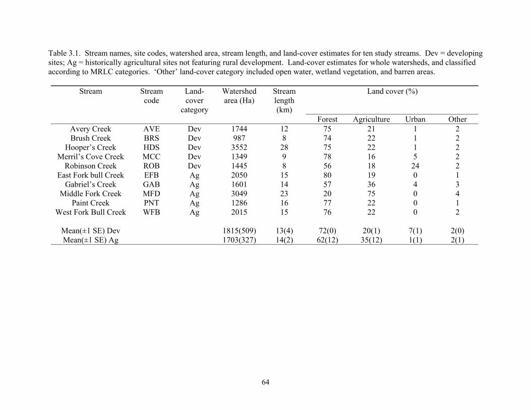
Table 3.1. Stream names, site codes, watershed area, stream length, and land-cover estimates for ten study streams. Dev = developing sites; Ag = historically agricultural sites not featuring rural development. Land-cover estimates for whole watersheds, and classified according to MRLC categories. ‘Other’ land-cover category included open water, wetland vegetation, and barren areas.

Stream Streamcode

Land-cover

category

Watershed area (Ha)

Stream length (km)

Land cover (%)

Forest Agriculture Urban OtherAvery Creek AVE Dev 1744 12 75 21 1 2 Brush Creek BRS Dev 987 8 74 22 1 2

Hooper’s Creek HDS Dev 3552 28 75 22 1 2 Merril’s Cove Creek MCC Dev 1349 9 78 16 5 2

Robinson Creek ROB Dev 1445 8 56 18 24 2 East Fork bull Creek EFB Ag 2050 15 80 19 0 1

Gabriel’s Creek GAB Ag 1601 14 57 36 4 3 Middle Fork Creek MFD Ag 3049 23 20 75 0 4

Paint Creek PNT Ag 1286 16 77 22 0 1 West Fork Bull Creek

WFB Ag 2015 15 76 22 0 2

Mean(±1 SE) Dev 1815(509) 13(4) 72(0) 20(1) 7(1) 2(0) Mean(±1 SE) Ag 1703(327) 14(2) 62(12) 35(12) 1(1) 2(1)

64

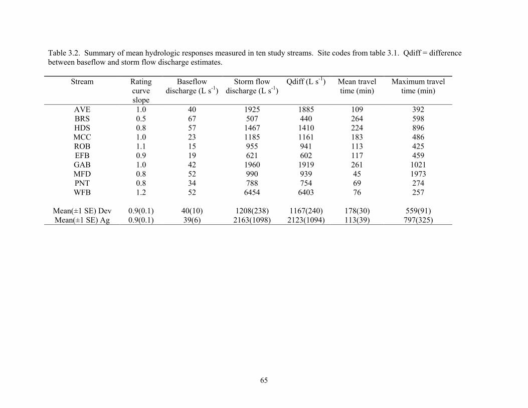
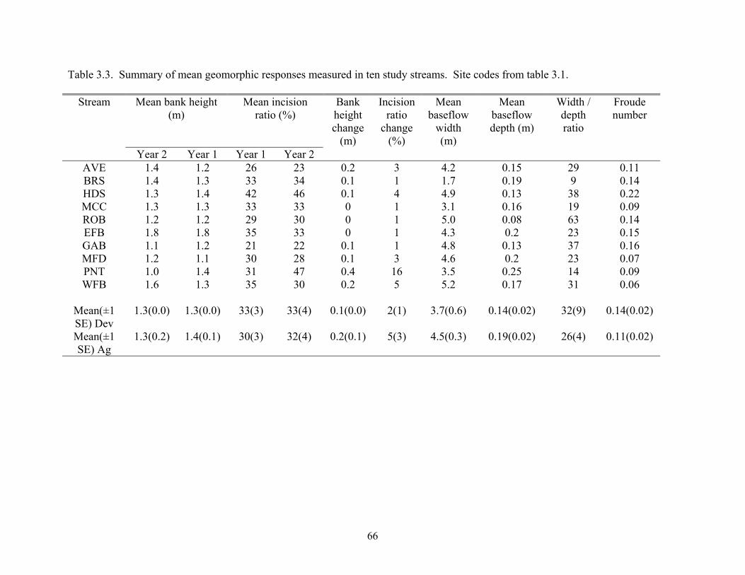
Table 3.2. Summary of mean hydrologic responses measured in ten study streams. Site codes from table 3.1. Qdiff = difference between baseflow and storm flow discharge estimates.

Stream Ratingcurve slope

Baseflow discharge (L s-1)

Storm flow discharge (L s-1)

Qdiff (L s-1) Mean traveltime (min)

Maximum travel time (min)

AVE 1.0 40 1925 1885 109 392BRS

0.5 67 507 440 264 598HDS 0.8 57 1467 1410 224 896MCC 1.0 23 1185 1161 183 486ROB 1.1 15 955 941 113 425EFB 0.9 19 621 602 117 459GAB 1.0 42 1960 1919 261 1021MFD 0.8 52 990 939 45 1973PNT 0.8 34 788 754 69 274WFB 1.2 52 6454 6403 76 257

Mean(±1 SE) Dev 0.9(0.1) 40(10) 1208(238) 1167(240) 178(30) 559(91) Mean(±1 SE) Ag 0.9(0.1) 39(6) 2163(1098) 2123(1094) 113(39) 797(325)

65

Table 3.3. Summary of mean geomorphic responses measured in ten study streams. Site codes from table 3.1.

Stream Mean bank height (m)

Mean incision ratio (%)

Bank height change

(m)

Incision ratio

change (%)

Mean baseflow

width (m)

Mean baseflow depth (m)

Width / depth ratio

Froude number

Year 2 Year 1 Year 1 Year 2 AVE 1.4 1.2 26 23 0.2 3 4.2 0.15 29 0.11BRS

1.4 1.3 33 34 0.1 1 1.7 0.19 9 0.14HDS 1.3 1.4 42 46 0.1 4 4.9 0.13 38 0.22MCC 1.3 1.3 33 33 0 1 3.1 0.16 19 0.09ROB 1.2 1.2 29 30 0 1 5.0 0.08 63 0.14EFB 1.8 1.8 35 33 0 1 4.3 0.2 23 0.15GAB 1.1 1.2 21 22 0.1 1 4.8 0.13 37 0.16MFD 1.2 1.1 30 28 0.1 3 4.6 0.2 23 0.07PNT 1.0 1.4 31 47 0.4 16 3.5 0.25 14 0.09WFB 1.6 1.3 35 30 0.2 5 5.2 0.17 31 0.06

Mean(±1 SE) Dev

1.3(0.0) 1.3(0.0) 33(3) 33(4) 0.1(0.0) 2(1) 3.7(0.6) 0.14(0.02) 32(9) 0.14(0.02)

Mean(±1 SE) Ag

1.3(0.2) 1.4(0.1) 30(3) 32(4) 0.2(0.1) 5(3) 4.5(0.3) 0.19(0.02) 26(4) 0.11(0.02)

66

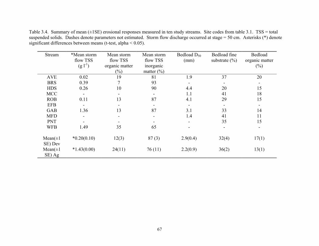
Table 3.4. Summary of mean (±1SE) erosional responses measured in ten study streams. Site codes from table 3.1. TSS = total suspended solids. Dashes denote parameters not estimated. Storm flow discharge occurred at stage = 50 cm. Asterisks (*) denote significant differences between means (t-test, alpha < 0.05).

Stream *Mean stormflow TSS

(g l-1)

Mean storm flow TSS

organic matter (%)

Mean storm flow TSS inorganic

matter (%)

Bedload D50 (mm)

Bedload fine substrate (%)

Bedload organic matter

(%)

AVE 0.02 19 81 1.9 37 20BRS

0.39 7 93 - - -HDS 0.26 10 90 4.4 20 15MCC - - - 1.1 41 18ROB 0.11 13 87 4.1 29 15EFB - - - - - -GAB 1.36 13 87 3.1 33 14MFD - - - 1.4 41 11PNT - - - - 35 15WFB 1.49 35 65 - - -

Mean(±1 SE) Dev

*0.20(0.10) 12(3) 87 (3) 2.9(0.4) 32(4) 17(1)

Mean(±1 SE) Ag

*1.43(0.00) 24(11) 76 (11) 2.2(0.9) 36(2) 13(1)

67

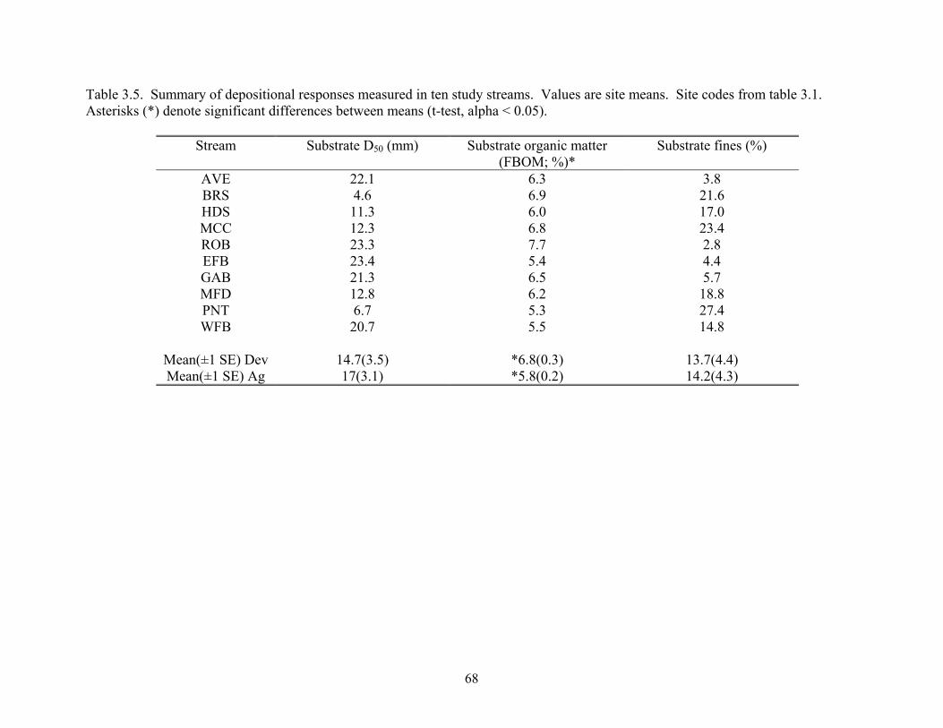
Table 3.5. Summary of depositional responses measured in ten study streams. Values are site means. Site codes from table 3.1. Asterisks (*) denote significant differences between means (t-test, alpha < 0.05).

Stream Substrate D50 (mm) Substrate organic matter (FBOM; %)*

Substrate fines (%)

AVE 22.1 6.3 3.8BRS

4.6 6.9 21.6HDS 11.3 6.0 17.0MCC 12.3 6.8 23.4ROB 23.3 7.7 2.8EFB 23.4 5.4 4.4GAB 21.3 6.5 5.7MFD 12.8 6.2 18.8PNT 6.7 5.3 27.4WFB 20.7 5.5 14.8

Mean(±1 SE) Dev 14.7(3.5) *6.8(0.3) 13.7(4.4) Mean(±1 SE) Ag 17(3.1) *5.8(0.2) 14.2(4.3)

68

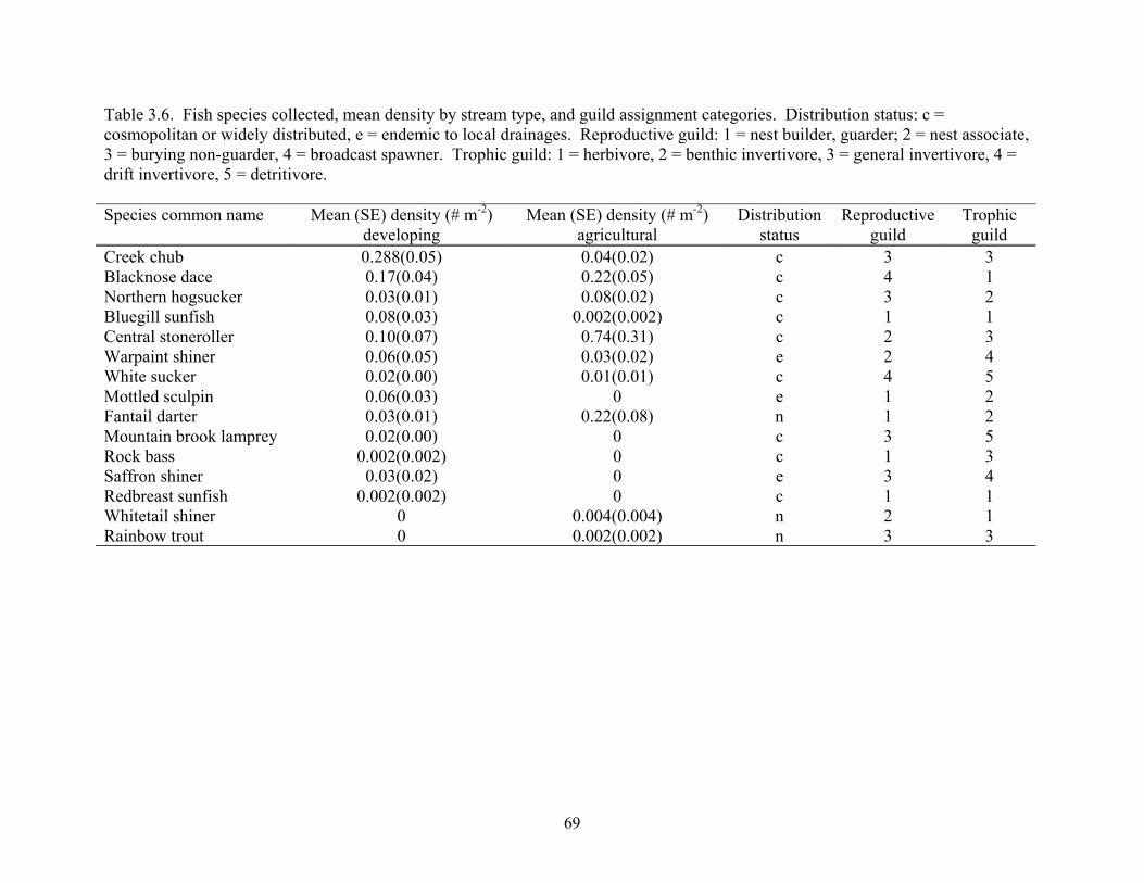
Table 3.6. Fish species collected, mean density by stream type, and guild assignment categories. Distribution status: c = cosmopolitan or widely distributed, e = endemic to local drainages. Reproductive guild: 1 = nest builder, guarder; 2 = nest associate, 3 = burying non-guarder, 4 = broadcast spawner. Trophic guild: 1 = herbivore, 2 = benthic invertivore, 3 = general invertivore, 4 = drift invertivore, 5 = detritivore. Species common name Mean (SE) density (# m-2)

developing Mean (SE) density (# m-2)

agricultural Distribution

status Reproductive

guild Trophic

guild Creek chub 0.288(0.05) 0.04(0.02) c 3 3 Blacknose dace 0.17(0.04) 0.22(0.05) c 4 1 Northern hogsucker 0.03(0.01) 0.08(0.02) c 3 2 Bluegill sunfish 0.08(0.03) 0.002(0.002) c 1 1 Central stoneroller 0.10(0.07) 0.74(0.31) c 2 3 Warpaint shiner 0.06(0.05) 0.03(0.02) e 2 4 White sucker 0.02(0.00) 0.01(0.01) c 4 5 Mottled sculpin 0.06(0.03) 0 e 1 2 Fantail darter 0.03(0.01) 0.22(0.08) n 1 2 Mountain brook lamprey 0.02(0.00) 0 c 3 5 Rock bass 0.002(0.002) 0 c 1 3 Saffron shiner 0.03(0.02) 0 e 3 4 Redbreast sunfish 0.002(0.002) 0 c 1 1 Whitetail shiner 0 0.004(0.004) n 2 1 Rainbow trout 0 0.002(0.002) n 3 3

69

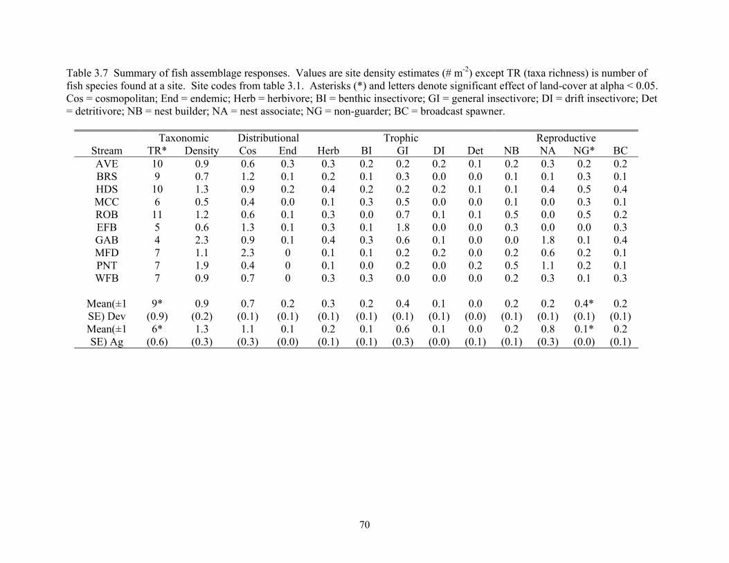
Table 3.7 Summary of fish assemblage responses. Values are site density estimates (# m-2) except TR (taxa richness) is number of fish species found at a site. Site codes from table 3.1. Asterisks (*) and letters denote significant effect of land-cover at alpha < 0.05. Cos = cosmopolitan; End = endemic; Herb = herbivore; BI = benthic insectivore; GI = general insectivore; DI = drift insectivore; Det = detritivore; NB = nest builder; NA = nest associate; NG = non-guarder; BC = broadcast spawner.

Taxonomic Distributional Trophic ReproductiveStream

TR* Density

Cos End Herb BI GI DI Det NB NA NG* BC

AVE 10 0.9 0.6 0.3 0.3 0.2 0.2 0.2 0.1 0.2 0.3 0.2 0.2BRS

9 0.7 1.2 0.1 0.2 0.1 0.3 0.0 0.0 0.1 0.1 0.3 0.1HDS 10 1.3 0.9 0.2 0.4 0.2 0.2 0.2 0.1 0.1 0.4 0.5 0.4MCC 6 0.5 0.4 0.0 0.1 0.3 0.5 0.0 0.0 0.1 0.0 0.3 0.1ROB 11 1.2 0.6 0.1 0.3 0.0 0.7 0.1 0.1 0.5 0.0 0.5 0.2EFB 5 0.6 1.3 0.1 0.3 0.1 1.8 0.0 0.0 0.3 0.0 0.0 0.3GAB 4 2.3 0.9 0.1 0.4 0.3 0.6 0.1 0.0 0.0 1.8 0.1 0.4MFD 7 1.1 2.3 0 0.1 0.1 0.2 0.2 0.0 0.2 0.6 0.2 0.1PNT 7 1.9 0.4 0 0.1 0.0 0.2 0.0 0.2 0.5 1.1 0.2 0.1WFB 7 0.9 0.7 0 0.3 0.3 0.0 0.0 0.0 0.2 0.3 0.1 0.3

Mean(±1 SE) Dev

9* (0.9)

0.9 (0.2)

0.7 (0.1)

0.2 (0.1)

0.3 (0.1)

0.2 (0.1)

0.4 (0.1)

0.1 (0.1)

0.0 (0.0)

0.2 (0.1)

0.2 (0.1)

0.4* (0.1)

0.2 (0.1)

Mean(±1 SE) Ag

6*(0.6)

1.3 (0.3)

1.1 (0.3)

0.1 (0.0)

0.2 (0.1)

0.1 (0.1)

0.6 (0.3)

0.1 (0.0)

0.0 (0.1)

0.2 (0.1)

0.8 (0.3)

0.1* (0.0)

0.2 (0.1)

70

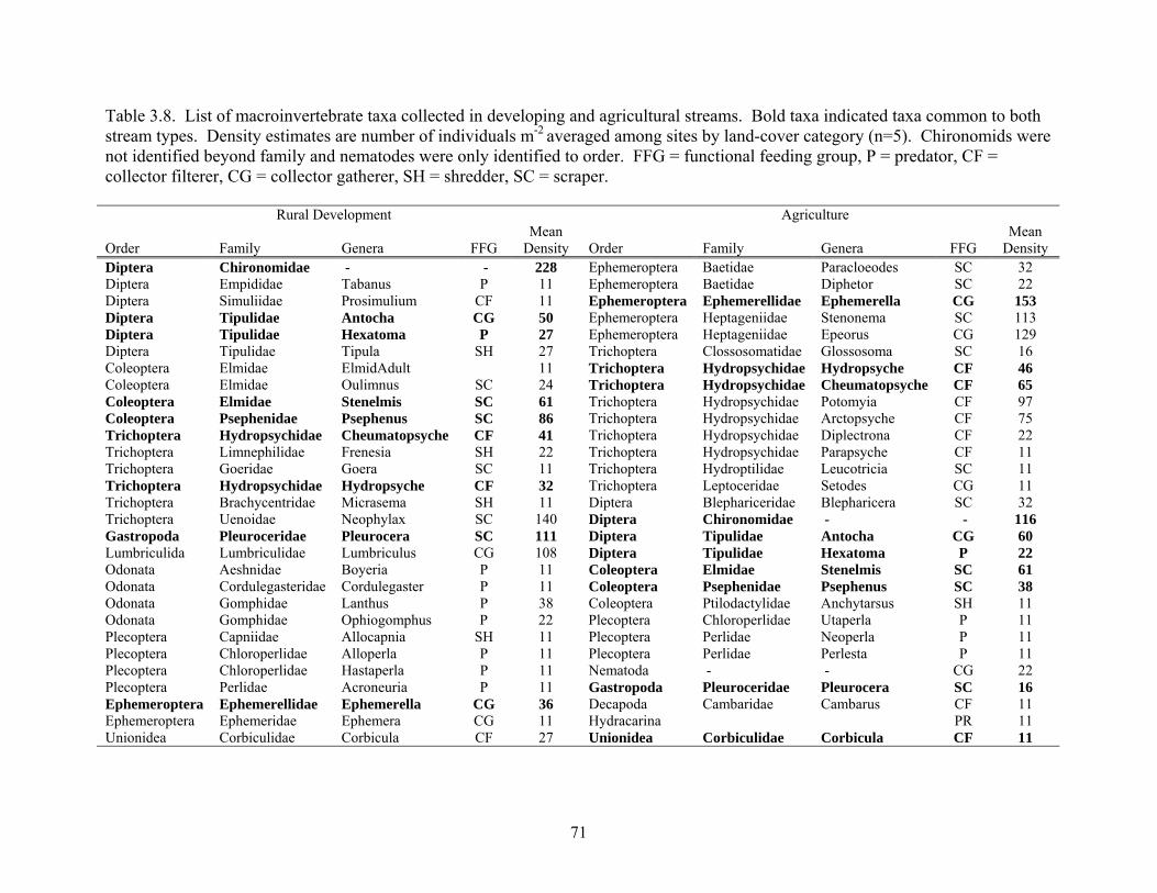
Table 3.8. List of macroinvertebrate taxa collected in developing and agricultural streams. Bold taxa indicated taxa common to both stream types. Density estimates are number of individuals m-2 averaged among sites by land-cover category (n=5). Chironomids were not identified beyond family and nematodes were only identified to order. FFG = functional feeding group, P = predator, CF = collector filterer, CG = collector gatherer, SH = shredder, SC = scraper. Rural Development Agriculture

Order

Family Genera FFG Mean

Density Order Family Genera FFG Mean

Density Diptera Chironomidae - - 228 Ephemeroptera Baetidae Paracloeodes SC 32

Diptera

Empididae Tabanus P 11 Ephemeroptera Baetidae Diphetor SC 22Diptera Simuliidae Prosimulium CF 11 Ephemeroptera

Ephemerellidae

Ephemerella

CG 153

Diptera Tipulidae Antocha CG 50 Ephemeroptera Heptageniidae Stenonema

SC 113Diptera Tipulidae Hexatoma P 27 Ephemeroptera Heptageniidae Epeorus CG 129Diptera Tipulidae Tipula SH 27 Trichoptera Clossosomatidae Glossosoma SC 16Coleoptera Elmidae ElmidAdult 11 Trichoptera Hydropsychidae Hydropsyche CF 46Coleoptera Elmidae Oulimnus SC 24 Trichoptera Hydropsychidae Cheumatopsyche

CF 65

Coleoptera Elmidae Stenelmis SC 61 Trichoptera Hydropsychidae Potomyia CF 97Coleoptera Psephenidae Psephenus SC 86 Trichoptera Hydropsychidae Arctopsyche CF 75Trichoptera Hydropsychidae

Cheumatopsyche

CF 41 Trichoptera Hydropsychidae Diplectrona CF 22

Trichoptera Limnephilidae

Frenesia SH 22 Trichoptera Hydropsychidae Parapsyche CF 11Trichoptera Goeridae Goera SC 11 Trichoptera Hydroptilidae Leucotricia

SC 11

Trichoptera Hydropsychidae Hydropsyche

CF 32 Trichoptera

Leptoceridae Setodes CG 11Trichoptera Brachycentridae

Micrasema SH 11 Diptera Blephariceridae Blepharicera SC 32

Trichoptera Uenoidae Neophylax SC 140 Diptera Chironomidae

- - 116 Gastropoda Pleuroceridae Pleurocera SC 111 Diptera Tipulidae Antocha CG 60Lumbriculida

Lumbriculidae Lumbriculus

CG 108 Diptera Tipulidae Hexatoma P 22

Odonata Aeshnidae Boyeria P 11 Coleoptera Elmidae Stenelmis SC 61Odonata Cordulegasteridae

Cordulegaster

P 11 Coleoptera Psephenidae Psephenus SC 38

Odonata Gomphidae Lanthus P 38 Coleoptera Ptilodactylidae Anchytarsus

SH 11Odonata Gomphidae Ophiogomphus

P 22 Plecoptera Chloroperlidae

Utaperla P 11

Plecoptera Capniidae Allocapnia SH 11 Plecoptera Perlidae Neoperla P 11Plecoptera Chloroperlidae Alloperla P 11 Plecoptera Perlidae Perlesta P 11Plecoptera Chloroperlidae

Hastaperla P 11 Nematoda - - CG 22

Plecoptera Perlidae Acroneuria P 11 Gastropoda Pleuroceridae Pleurocera SC 16Ephemeroptera

Ephemerellidae

Ephemerella CG 36 Decapoda Cambaridae Cambarus CF 11

Ephemeroptera

Ephemeridae Ephemera CG 11 Hydracarina PR 11 Unionidea Corbiculidae Corbicula CF 27 Unionidea Corbiculidae Corbicula CF 11

71

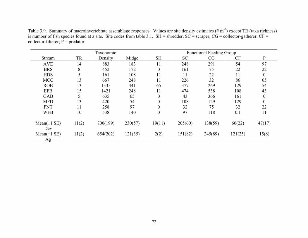
Table 3.9. Summary of macroinvertebrate assemblage responses. Values are site density estimates (# m-2) except TR (taxa richness) is number of fish species found at a site. Site codes from table 3.1. SH = shredder; SC = scraper; CG = collector-gatherer; CF = collector-filterer; P = predator.

Taxonomic Functional Feeding Group Stream

TR Density Midge SH SC CG CF P

AVE 14 883 183 11 248 291 54 97BRS

8 452 172 0 161 75 22 22HDS 5 161 108 11 11 22 11 0MCC 13 667 248 11 226 32 86 65ROB 13 1335 441 65 377 269 129 54EFB 15 1421 248 11 474 538 108 43GAB 5 635 65 0 43 366 161 0MFD 13 420 54 0 108 129 129 0PNT 11 258 97 0 32 75 32 22WFB 10 538 140 0 97 118 0.1 11

Mean(±1 SE) Dev

11(2) 700(199) 230(57) 19(11) 205(60) 138(59) 60(22) 47(17)

Mean(±1 SE) Ag

11(2) 654(202) 121(35) 2(2) 151(82) 245(89) 121(25) 15(8)

72

¯

0 5 10 Kilometers

FrenchBroadRiver

Agriculture sites

Developing sites

Asheville

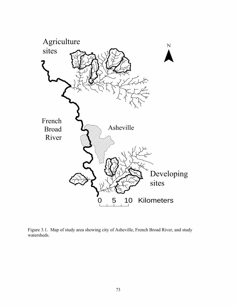
Figure 3.1. Map of study area showing city of Asheville, French Broad River, and study watersheds.

73

TSS

conc

entra

tion

(g l-

1)

0.0

0.8

1.6

Dev Ag

Subs

trate

FB

OM

(%)

0

4

8

p < 0.001

p = 0.027

A

B

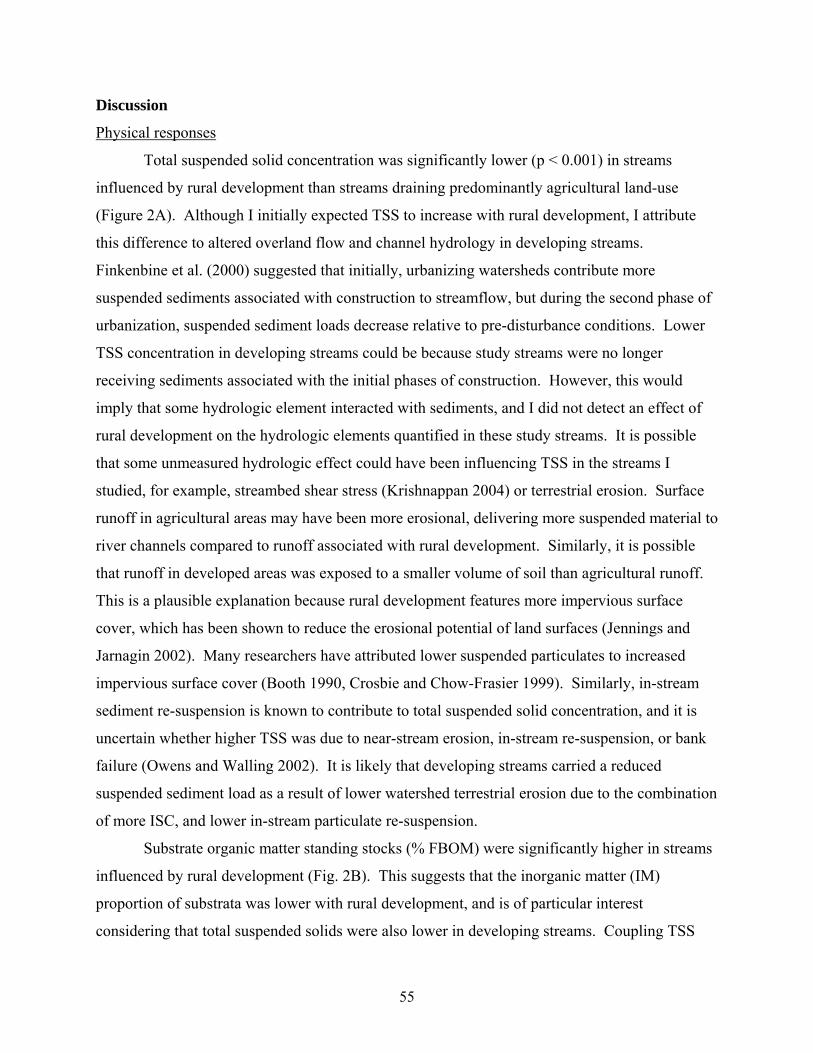
AB

Figure 3.2. Mean (± 1 SE) TSS and FBOM concentration in rural vs. agricultural streams. Letters denote significant differences between stream type. Dev = developing sites, Ag = agricultural sites.

74

Fish

taxa

rich

ness

0

6

12

Dev Ag

NG

den

sity

(# m

-2)

0.00

0.25

0.50

p = 0.017

p = 0.007

A

A

B

B

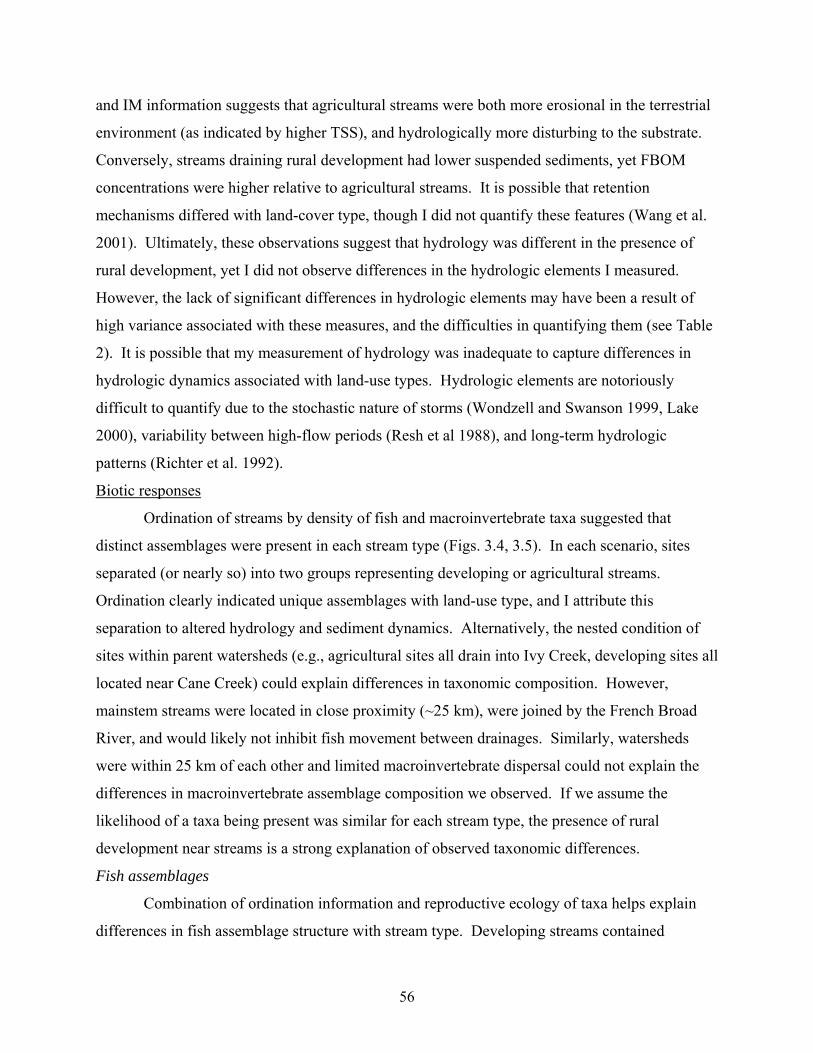
Figure 3.3. Mean (± 1 SE) fish TR and NG density in rural vs. agricultural streams. Dev = developing sites, Ag = agricultural sites.

75

Figure 3.4. Detrended correspondence analysis of streams by fish species density. Triangles d

AVEHDS ROB

MCC

BRS

PNTMDS

GAB

EFBWFB

Creek Ch

BlacknosNorthern

Bluegill

Central

Warpaint

White su

Mottled

Fantail

Mountain

Rock Bas

Saffron

Redbreas

Whitetai

Rainbow

Axis 1

Axi

s 2

indicated locations of streams in the hypothetical space defined by species distribution. Dashecircles indicate grouping of sites by land-use category. Site codes are from table 3.1. Fish common names are truncated to 8 letter abbreviations and can be found in Table 3.6.

76

Axis 1

WFB

EFB

MFD

PNT

GAB ROB

MCC

HDSAVE BRS

Oligo

ElmAdult

Stenelmi PsephenuOulimnus

AnchytarBlephari

Chironom

Antocha

DicranotHexatoma

Tipula

Tabanus

Prosimul

Diphetor

Paracloe

Ephemera

Ephemerella

Epeorus

Stenonem

Nigronia

Boyeria

Corduleg

Lanthus

Omphigom

Allocapn

Alloperl

Hastaper

Utaperla

Acroneur

Neoperla

Perlesta

Micrasem

Glossoso

Glossoso

Goera

Arctopsy

Cheumato

Dip lectr

Hydropsy

Parapsyc

Potomyia

Leucotri

SetodesFrenesia

Neophyla

Cambarus

PleuralSOtherSna

Hydrocar

NematodaCorbicu l

Axi

s 2

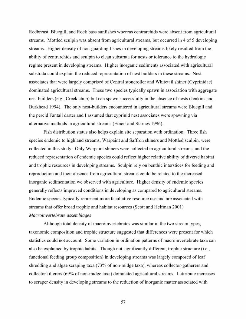
Figure 3.5. Detrended correspondence analysis ordination of streams by macroinvertebrate density. Dashed circles indicate grouping of sites by land-use category. Dotted circles group taxa common to one ordination location. Site codes are from table 3.1. Macroinvertebrate names are truncated to 8 letter abbreviations and can be found in Table 3.8.

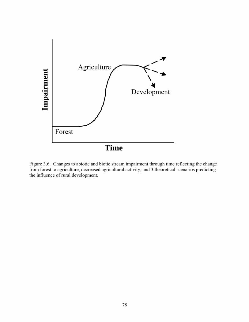
77

Time

Forest

Agriculture

Development

Impa

irm

ent

Figure 3.6. Changes to abiotic and biotic stream impairment through time reflecting the change from forest to agriculture, decreased agricultural activity, and 3 theoretical scenarios predicting the influence of rural development.

78

Chapter 4: Multivariate versus bivariate analysis of land-cover disturbance to stream biota Abstract

I introduce the land-cover path (LCC) hypothesis as a conceptual framework to organize

the transfer of land-cover disturbance to stream biota through a cascading gradient of

intermediate abiotic variables. Selected abiotic variables represent key ecosystem features that

transform disturbance and pass a reorganized effect to the next variable where the process

repeats until ultimately affecting biota. I hypothesized that land-cover affects stream biota

indirectly through a hierarchy of stream abiotic components that transform disturbance to biota.

I measured 31 hydrologic, geomorphic, erosional, and substrate variables and 26 biotic responses

that have been associated with land-use disturbance. Regression analyses reduced this set of

variables to include only those abiotic variables that responded to land-cover and/or affected

biota. From this reduced variable set, hypotheses were generated that organized the disturbance

pathways linking land-cover to each biotic response. I identified a multivariate path model for

each biotic response that illustrated the pathway through which land-cover influenced physical

variables and ultimately biota. Paths were tested for predictive ability and goodness-of-fit using

path analysis and the Amos® software program. Biota were influenced both directly (i.e.,

bivariate linear regressions) and indirectly (i.e., multivariate path analyses) by near-stream urban,

agricultural, and forest land-cover as well as by hydrologic, geomorphic, erosional, and

depositional substrate features. Multivariate models (indirect effects) were compared to bivariate

models (direct effects). Indirect pathways generally predicted biotic responses better than direct

effects and always explained more of the associated variance by including intermediate abiotic

variables. Path models suggested that fish and macroinvertebrates were influenced by near-

stream agricultural disturbance that cascaded through channel geomorphic elements including

bank height, incision ratio, and width / depth ratio, inorganic sediment loads, and substrate size

and organic matter content. Some bivariate models significantly predicted biotic responses but

were not easily translated ecologically. My results suggest that intermediate abiotic variables

were important in propagating land-cover disturbance to biota and usually provided more

information than bivariate relationships. More generally, the land-cover cascade concept and

experimental framework was useful in explaining variation in biotic responses associated with

79

the propagation of anthropogenic disturbance through intermediate abiotic ecosystem

components.

Introduction

The cascade approach could be useful in ecosystem research to organize multivariate

interactions occurring at multiple spatial scales. Much is known about the disturbance response

of individual ecosystem components, but how components interact, and how disturbance is

transformed, is largely unknown (Lake 2000). Ecosystem response to disturbance is difficult to

study due to the varying nature, intensity, and duration of both disturbance and ecosystem

responses. As the spatial scale of research gets larger the number of important variables or the

scale of relevant variables can also increase and weaken our ability to identify mechanisms

(Strayer et al. 2003). Ecosystems are also difficult to replicate and the variance associated with

ecosystem measures are difficult to quantify. As a result, much of what we know about

anthropogenic disturbance to streams has come from small-scale studies that make bivariate

inferences of ecosystem scale effects (Downes et al. 2002).

Many bivariate studies have shown that land-cover disturbance induces a series of direct

effects to ecosystem structure and function (Meyer and Turner 1992, Jacobson et al. 2001).

Land-cover changes have been shown to induce hydrologic, geomorphic, erosional, and biotic

responses (Waters 1995, Richards et al. 1996, Harding et al. 1999, Cuffney et al. 2000, Lee and

Bang 2000). Bivariate studies typically use regression or correlation analyses to identify

relationships between land-cover and abiotic or biotic responses but cannot explain the

disturbance pathways involved and thus cannot be used to identify mechanisms. Conclusions

generated from such studies have limited use in generalizing relationships among multiple

variables and often report direct, bivariate effects of land-cover on biota but do not quantitatively

link biotic responses, land-cover, and intermediate variables. The bivariate approach is limited

when research questions demand consideration of multiple spatial scales and when significant

relationships may involve intermediate variables. A cascade approach to ecosystem disturbance

study will help link intermediate variables or acting to propagate land-cover disturbance to biota

indirectly (i.e., indirect effects). Cascades imply multivariate path models that join land-cover

effects and biota through at least one intermediate variable, or link. Path models may also

identify relationships among response variables that facilitate the identification of mechanisms

involved in transforming landscape-scale disturbance to biota.

80

Here I propose a cascade approach to organize how land-cover disturbance is transformed

via interacting abiotic variables across multiple spatial scales to ultimately affect stream biota

(sensu Frissell et al. 1986; Fig. 4.1). The land-cover cascade (LCC) is a novel design used to

organize the series of intermediate variables through which land-cover disturbance energy

‘flows’ along a reducing temporal and spatial gradient before influencing biota (Montgomery

1999). Generally, the LCC describes a 3-tiered hierarchy among land-cover, physical elements,

and biotic responses. I constructed individual cascades for each biotic response and tested the

predictive ability of multivariate models to bivariate comparisons between land-cover or abiotic

variables and biotic responses. To build each LCC model I identified important intermediate

abiotic variables between land-cover and biota as being hydrologic, geomorphic, erosional, and

substrate elements. I used variables known to respond to land-cover disturbance and/or induce

biotic responses to build multivariate models describing relationships among land-cover, biota,

and physical ecosystem elements. I considered disturbance effects as originating with land-cover

and being transformed by intermediate abiotic variables (i.e., links) to produce a terminal biotic

response. Some of the disturbance would be realized at each intermediate variable and some

transferred to the next link along the path. Each link is considered a necessary step in the

complete translation of land-cover disturbance to a particular biotic community response.

I hypothesized that land-cover disturbance would follow a cascade pattern whereby

disturbance was transformed to the next-smaller spatial scale through physical response variables

and that cascades would continue until eventually affecting stream biota. I predicted that each

bivariate link within a cascade could be quantified and the overall predictive value of a cascade

assessed using structural equation modeling (SEM) to quantify cascades as path models. To

assess the value of LCC models I compared SEM results to bivariate comparisons (i.e.,

regression and correlation) between land-cover and individual biotic responses. I predicted that

biotic responses would be better explained by multivariate (i.e., indirect effects explained by the

LCC and SEM; path models) than bivariate (i.e., direct effects) models. I expected biota to

respond strongly to altered substrate and sediment dynamics associated with higher agricultural

or urban land-cover.

81

Methods

Study sites

To develop testable LCC models I measured physical and biotic elements in ten 3rd – 4th

order streams in the Blue Ridge physiographic province in western North Carolina that had been

historically influenced by row crop and grazing agriculture. The streams were similar in length,

gradient, and underlying geology. Watershed areas varied from 1000 – 3500 Ha ( x = 1907 ±

256 ha). All watersheds contained active agricultural areas since at least 1950, and included 21 –

77 % ( x = 47 ± 18 %) agriculture and 16 – 62 % ( x = 40 ± 14 %) forest as of 1993 (Herman

1996, USCB 2002).

Land-cover definition

Land-cover circa 1993 was estimated from National Land-cover Dataset (NLCD; USDI

2002). Whole watershed land-cover classification was calculated as the percentage of a land-

cover type in the entire watershed area. Twenty-nine NCLD land-cover categories were reduced

to four. Agriculture included active row crop or grazing areas and old fields. Urban included

urban and rural areas in addition to roads and other elements of human infrastructure. Forest

combined most vegetation categories, and other categories included open water, barren, and

others that did not fit into the previous categories.

I considered land-cover along a spatial gradient from near-stream to whole watershed

areas. Riparian corridors of 100-m width were estimated in a GIS and land-cover percentages

defined within. To examine land-cover along a continuum of spatial proximity to stream

channels, overland flow travel time zones (TTZs) were used to constrain the area in which land-

cover percentages were estimated, and thus how independent variables were defined. Travel

time estimates were calculated using a GIS and defined by gradient, surface roughness, average

rainfall, and other criteria (C.L. Burcher, Chapter 2 this dissertation). Travel time zones ranging

from 30 to 300-min were used to delimit spatial zones ranging from proximal, near-stream areas

to the whole watershed. Percent land-cover in agriculture, light urban, heavy urban, and forest

categories were estimated in each of ten TTZs.

Quantifying physical and biotic characteristics

I quantified several metrics that I hypothesized would be important components involved

in the LCC of study streams. Metrics were established to capture both the spatial and temporal

range of known physical responses that have been shown or inferred to contribute to biotic

82

responses to land-cover change (sensu Ward 1989; Fig. 4.1). Hydrologic metrics captured

landscape scale phenomena including discharge and overland-flow travel-time estimates.

Geomorphic metrics were calculated from multiple channel cross-section surveys, digital

elevation models, and line-transect discharge measurements. Erosional metrics were suspended

and bedload sediment concentration and percent fine benthic organic matter (FBOM). Substrate

metrics quantified particle size, composition, and percent substrate FBOM.

Fish were sampled during August in 2002 using single pass backpack electrofishing

along 100-m stream reaches. Reaches were subdivided into 1 to 10-m sections using natural

breaks in habitat units as boundaries between sub-units. Electrofishing herded fish into a seine

(5-mm mesh) at the downstream end of each sub-unit. Fish were collected and identified to

species after each sub-unit was sampled and returned downstream. Density was estimated as the

number of individuals collected per stream area sampled (100-m X average stream width; # m-2).

Fishes were assigned to distributional, reproductive, and trophic guilds based on available

information for each species. Distribution status reflects historic occurrence of a species within

and across drainages (Scott and Helfman 2001). Cosmopolitan species are widely distributed

through a drainage and span stream order and habitat gradients. Endemic species are often only

found in a small portion of a drainage often in a very localized area. I considered endemic fishes

in the southern Appalachian region to be associated with highland areas, or higher gradient,

lower-order streams and to have limited geographic distributions relative to cosmopolitans (Scott

and Helfman 2001).

Fishes were assigned to reproductive guilds based on known spawning habits of each

species. Fishes vary in their mode of reproduction and can build nests, guard eggs, or simply

broadcast eggs across the benthos. I placed species into 1 of 5 reproductive guilds (Jenkins and

Burkhead 1994, Etnier and Starnes 1993). Nest builders (NB) build and guard nests and

included centrarchids and the Fantail darter. Nest associates (NA) often spawn in association

with pebble mounds organized by another species and included Whitetail shiner, Warpaint

shiner, and Central stoneroller minnows. Burying non-guarders (NG) hide eggs in substrate

without further parental care and included species from several families. Broadcast spawners

spread eggs and milt over an area of substrate without burying or providing parental care and

included Blacknose dace and White suckers.

83

Fish feeding habits were also used to categorize species by feeding guild based on

recorded knowledge of each species (Jenkins and Burkhead 1994, Etnier and Starnes 1993).

Herbivores are fishes feeding primarily on living plant material, algae, and detritus and included

Bluegill, Redbreast sunfish, Whitetail shiner and Blacknose dace. Invertivores prefer insects and

crustaceans and were subdivided by the portion of the water column prey is taken. Benthic

invertivores pick prey items from substrata, often have specialized subterminal mouths designed

for bottom feeding and included the Northern hogsucker. Drift invertivores lie-and-wait for

drifting prey to be delivered to them, and included Warpaint and Saffron shiners. General

invertivores are species known to collect prey items from multiple locations within a stream and

included Creek chub, Central stoneroller, Rock bass, and Rainbow trout. Detritivores feed

primarily on detritus matter and included White sucker and Mountain brook lamprey.

Macroinvertebrates were collected during late April 2003 using twenty quantitative

(Surber, 500-µm mesh, 0.09 m2, 1.8 m2 total area sampled per 100-m reach). Density (# m-2)

was estimated from individual samples and average density by taxa calculated for each stream.

Macroinvertebrates were preserved in 80% ethanol and identified to the lowest possible

taxonomic level (typically genus). Taxa were placed into functional feeding groups (FFG) based

on the classification by Merrit and Cummins (1996) or expert opinion of macroinvertebrates in

southern Appalachian streams. Functional feeding groups included collector-filterers and

collector-gatherers known to remove particulate matter from the water column, shredders that

feed on decaying leaves, scrapers that have specialized mouthparts for removing algae from rock

surfaces, and predators that consume other animals. I did not consider ontogenetic changes to

feeding habit associated with small instars and assumed that individuals of a species could be

classified into a single FFG.

Statistical analyses; direct and indirect effects

Variables in were organized according to the conceptual LCC hierarchy (Fig. 1). Thirty-

six land-cover variables (twelve each in agriculture, forest, and urban categories) were always

considered independent variables. Physical variables (30 total; 6 hydrologic, 10 geomorphic, 11

erosional, and 3 substrate) were considered both dependent variables affected by land-cover and

independent variables affecting other physical variables and biotic responses. Biotic variables

(21 total; 13 fish and 8 macroinvertebrate) were always considered dependent variables, either

directly on land-cover or indirectly through physical variables.

84

Every possible pairwise combination of variables was analyzed with simple linear

regression. Land-cover was compared to every other physical and biotic variable (51 total) for a

total of 1836 comparisons. All physical variables were compared with each biotic variable in

630 comparisons. Ecologically significant variables were defined as those that were

significantly correlated (p < 0.05) to at least one other variable and contained no visible outliers

in scatter-plots. Significant relationships were further assessed to determine whether they were

ecologically feasible. For example, if a bivariate model predicted that land-cover would be

influenced by substrate size then that model would be omitted based on the seemingly impossible

scenario implied. Resulting variables represented the strongest potential among measured

variables to either link land-cover to biota or predict biotic responses directly (i.e., a direct effect

of land-cover to biota). Significant bivariate regressions between land-cover and biotic

responses were compared to the path model that predicted the same biotic response.

Path analysis

Path analysis is a form of structural equation modeling and a statistical technique that

allows researchers to relate variables and their inferred influence sequentially (Shipley 2000).

Similar to multivariate regression, path analysis considers dependent variables potentially

influenced by multiple independent variables but allows each independent variable to interact

with one another. Path analysis decomposes the total variation in a dependent variable

associated with all other variables in a model. Unlike linear or multiple regression methods,

however, path analysis also allows consideration of interaction or correlation among independent

variables along hypothetical paths. Path analysis provides coefficients similar to r2 that indicate

how much variation in response variables is explained by each independent variable and the

entire model. Path analysis also provides correlation coefficients for each bivariate pair

providing both direction and a measure of relatedness.

Path models were constructed and assessed using Amos® version 5.0 to decompose direct

(i.e., bivariate) and indirect (i.e., multivariate path) effects of each path model variable on each

biotic response (Arbuckle 2003). Path models were built according to significant direct

relationships identified by linear regression whereby variables related to one another in a

bivariate sense (i.e., significant with linear regression) were combined to connect land-cover to

biota through related abiotic variables. For example, if agriculture was significantly linked (i.e.,

significant regression) to baseflow discharge and discharge was linked to fish taxa richness, a

85

path model could be built linking agriculture to discharge and discharge to taxa richness. Path

analysis would calculate the correlation between each variable pair and assess the overall

predictive capacity of the model. Each link (i.e., bivariate comparison) was known to be

significant based on the underlying linear regression analysis completed prior to model building

but whether or not a path model would be significant depended on the overall strength of all

variables in a model.

Path models indicated the structure of cascading physical and biotic variables that were

hypothesized to affect a particular biotic response (Fig. 4.2). Paths included at least 3 variables,

but could include all significant relationships. For example, total fish density was hypothesized

as being affected by agriculture as delimited within 60-min travel time zones that initially (i.e.,

prior to affecting fish density) induced a change to bank height and subsequently influenced

baseflow total suspended solids (TSS) percent inorganic matter. Models provided measures of

direct and indirect effects and indicated the percent variance (analogous to overall r2 in linear

regression) in a biotic response that was explained by an entire pathway. Each model was tested

for goodness of fit using chi-squared analysis, root mean squared error approximation (RMSEA),

and the normed fit index (NFI) output from Amos® (Arbuckle 2003).

Results

Simple linear regression reduced 36 land-cover variables and 51 physical and biotic

variables to 11 land-cover, 16 physical, and 15 biotic variables (Table 4.1). The reduced set of

variables was used to construct LCC models that were tested using path analysis. Linear

regression between land-cover and biotic responses were compared to path analysis results and

the utility of each model considered.

Path models

Thirteen of twenty-two hypothesized path models predicted six fish and seven

macroinvertebrate responses and described significant cascades between land-cover and biota

(Fig. 4.2). The remaining nine models tested were not significant with Amos® but were

compared with significant bivariate regression models for similar land-cover / biotic response

comparisons to assess the relative predictive ability of multivariate versus bivariate approaches.

Each significant path model path began with land-cover effects and included at least one physical

response. Direct (i.e., bivariate) and indirect (i.e., multivariate) effects were decomposed to

estimate the predictive values (analogous to overall r2) for each path model and for each variable

86

within a path model (Table 4.2). Multivariate path models explained between 41 % (fish non-

guarder density) and 92 % (fish taxa richness and total density) of the variance observed in biotic

responses (Fig. 4.2). All path models fit according to chi-square (X2) analyses, although some

models failed RMSEA and NFI fit tests (Table 4.3). Goodness-of-fit tests compared the

hypothesized model to data covariance structure to determine how well the hypothesized model

fit the actual data. X2 significance is often considered sufficient criteria to consider a model

meaningful and I considered this acceptable despite the failure of some models’ fit indicated by

RMSEA and NFI (Shipley 2000, Arbuckle 2003, Riseng and Wiley 2004).

Six land-cover, 2 hydrologic, 3 geomorphic, 1 erosional, 3 substrate, 5 fish, and 7

macroinvertebrate variables were included in path models. The remaining pairwise relationships

included variables that did not participate in any path model and were not considered in bivariate

comparisons of land-cover and biota (Appendices A, B). Fish and macroinvertebrate responses

were generally influenced by near-stream land-cover (i.e., described with in 60, 90, or 120-min

TTZs or 100-m corridors) although watersheds scale agriculture was important in predicting a

change to the density of fish nest associates. Baseflow discharge and the slope of discharge /

stage rating curves were significant in several path models including macroinvertebrate total

density and collector filterer density but, in general, hydrologic elements were not predictive and

did not significantly affect the influence of land-cover to fish responses. Mean bank height

measured in year 1, the change to bank incision ratio over 1 year, and the width / depth ratio of

baseflow depth were important geomorphic elements in all but two path models. Percent

stormflow TSS inorganic matter was the only significant erosional element and was a key entity

in path models explaining fish assemblage responses but not included in any macroinvertebrate

path. Substrate metrics were important in several models to both fishes and macroinvertebrates.

Fish responses

Path models significantly predicted three fish taxonomic metrics. The path model that

summarized the influence of near-stream agriculture on stormflow inorganic matter explained

ninety-two percent of the variation in fish taxa richness among streams (IM; Fig. 4.2a). The fish

taxa richness path model suggested that agriculture described within 100-m riparian corridors

positively influenced storm flow inorganic matter concentration, which in turn negatively

influenced fish taxa richness. In other words, higher near-stream agriculture negatively

influenced fish taxa richness via the intermediate influence on storm flow IM. The fish total

87

density path model significantly explained the positive influence of near-stream agriculture to

bank height and the direct effects of baseflow TSS inorganic matter (Fig. 4.2b; 92 % variance in

total density explained). Density of cosmopolitan fishes (i.e., widely distributed as opposed to

localized in distribution) was explained (91%) by a combination of agriculture bank height, and

suspended inorganic particles (Fig. 4.2c). The cosmopolitan fish path model indicated that both

near-stream (i.e., 60-min travel time zones) and large-scale (i.e., whole watershed) agriculture

positively influenced bank height (i.e., streams were deeply incised) and baseflow TSS organic

matter. Deeper banks negatively influenced, whereas suspended inorganic TSS positively

influenced cosmopolitan fish density.

Fish metrics that summarized reproductive behavior and associated habitat preferences

were also significantly modeled using path analysis. Forty-one percent of the variation in fish

non-guarder density (fishes that do not guard their eggs after spawning) was explained by a path

model whereby near-stream agriculture (i.e., described within 60-min travel time zones)

negatively influenced the incision ratio change of stream channels (i.e., whether bank slope

changed between sample years), which negatively influenced percent organic matter (OM) in

substrata, which positively influenced fish non-guarder density (Fig. 4.2d). In other words,

increased agriculture was associated with bank erosion that was related to a higher ratio of

substrate organic matter (as compared to IM). Lower IM was significantly related to higher fish

non-guarder density. Similarly, increased fish nest-associate density (i.e., fish that spawn in the

presence of nests built by other species) was predicted (88%) by watershed-scale agriculture

positively influencing TSS % IM (41%; Fig. 4.2e). Combined, models summarizing fish

reproductive structure suggested that the reproductive structure of fish assemblages was altered

by inorganic sediments and channel shape associated with near-stream and whole-watershed

agriculture.

One metric summarizing trophic structure of fish assemblages was significantly predicted

by path analysis. Density of herbivorous fishes was higher in association with urban land-cover

described within 120-min travel time zones. Urban land-use positively influenced width / depth

ratios (i.e., streams were wide and shallow) which led to a decrease in substrate % fines and an

increase to fish herbivore density (49 % variance in fish herbivore density explained; Fig. 4.2f).

Fish responses, in general, were predicted by near-stream agriculture (i.e., as described

within 60 to 120-min travel-time zones) and were not affected by hydrologic variables in any

88

path model. Bank height, incision ratio change, and width / depth ratio were important

predictors of total, cosmopolitan, non-guarder, and herbivore fish density. Percent IM was

important in each path except for herbivore and non-guarder density paths. Substrate inorganic

matter and percent fines were only predictive to non-guarder and herbivore density respectively.

Macroinvertebrate responses

Three taxonomic macroinvertebrate metrics; taxa richness, total density, and midge

density were significantly predicted by path models. Higher taxa richness was associated with

lower cosmopolitan fish density and by higher bank height associated with higher near-stream

agriculture (49%; Fig. 4.2g). Fifty-seven percent of variation in macroinvertebrate total density

was explained by a path model that summarized the influence of near-stream agriculture and

urban land-cover (Fig. 4.2g). Macroinvertebrate total density was lower with higher agriculture

due to lower rating curve slope values and smaller D50. Higher urban land-cover, however,

appeared to be positively related to total density by inducing wider, shallower streams (i.e.,

higher w/d ratios) and lower % fine substrata. Eighty percent of the variation in midge density

among sites was explained by a path model summarizing the negative influence of near-stream

agriculture (i.e., described within 60-min travel time zones), higher baseflow discharge, and

higher density of fish nest associates (Fig. 4.2i). Midge density appeared to negatively respond

to higher agriculture, deeper stream channels, and predation by nest associates.

Four significant path models were developed that predicted responses of

macroinvertebrate functional feeding groups (FFGs) to land-cover. Macroinvertebrate shredders,

dependent on allochthonous-derived organic matter (e.g., leaves) were positively influenced by

agriculture. Forty-eight percent of the variation in shredder density among sites was explained

by a model linking higher agriculture (described within 60-min travel time zones) to bank

movement or erosion (incision ratio change) and higher percent benthic organic matter (Fig.

4.2j). Macroinvertebrate scraper density responded similarly to shredders in a model explaining

46% of the variation in scraper density (Fig. 4.2k). Scrapers also appeared to benefit from lower

urban activity in 120-min travel time zones and the intermediate influence of urban activity on

substrate OM. A positive influence of urban land-use was also apparent in the model predicting

collector-filterer density (Fig. 4.2l). Collector-filtering macroinvertebrate density was lower in

association with higher agriculture and lower urban land-cover described within 120-min travel

time zones. Agriculture was negatively related to rating curve slope and D50 was positively

89

correlated to urban land-use and w/d ratios. In other words, D50 was negatively influenced by

agriculture and the associated influence on discharge but also positively by urban land-use

influencing narrower and deeper stream channels. Urban land-cover negatively influenced

collector-gathering macroinvertebrate density (Fig 4.2m). A cascading path model indicated that

higher urban activity was associated with wider, shallower streams (i.e., higher w/d ratio) and

lower % fine substrata and explained 70% of the variance in collector-gatherer density.

Agriculture and urban land-cover altered hydrology features, substrate D50, and percent

fine substrates. Agriculture most strongly influenced macroinvertebrate total density and the

presence of agriculture contributed to deeper, flashier streams dominated by small substrates.

Macroinvertebrate responses were generally predicted by near-stream agriculture but total,

scraper, collector-filterer, and collector-gatherer density was affected by urban land-cover. Near-

stream forest cover positively influenced scraper density. Stream hydrology, specifically rating

curve slope, affected total density and density of collector filterers. Similar to fishes,

macroinvertebrates responded to geomorphic features including bank height, incision ratio

change, and width / depth ratio. Substrate characteristics were particularly important in

predicting macroinvertebrate responses except for taxa richness and midge density.

Bivariate analyses

Sixty-nine pairwise combinations of all possible variable combinations were significant

with linear regression (Table 4.2, Appendix B). I considered these relationships to be

ecologically significant (i.e., direct effects) where land-cover or a physical response explained

more than 40% of the variation (i.e., r2 > 0.4) in a physical or biotic response. I chose 40% as the

rejection level to be conservative enough to consider entities that may contribute to a larger

model but permissive enough to reduce the number of entities I considered. Low correlation

(i.e., 40 to 60 %) has limited meaning in a bivariate sense but whether a single variable would be

more useful in multivariate models was unknown. I wanted to eliminate enough variables to

design practical multivariate models but be conservative enough to maintain variables that could

potentially contribute to larger models.

Land-cover significantly explained variation in 4 fish and 5 macroinvertebrate responses

(Table 4.2). Density of cosmopolitan fishes was negatively related to higher forest cover within

100-m riparian corridors (p = 0.042, r2 = 0.422). Fish detritivore density was negatively

influenced by higher agriculture within 60-m TTZs (p = 0.005, r2 = 0.642). Density of nest

90

associate fishes was positively associated with 100-m buffer agriculture (p = 0.024, r2 = 0.489).

Non-guarding fish density was influenced negatively by forest cover (90-min TTZs; p = 0.013,

r2 = 0.556) and urban land-cover (60-min TTZs; p = 0.012, r2 = 0.564). Midge density was

significantly predicted by near-stream agriculture (100-m corridors; negative relationship; p =

0.021, r2 = 0.508) and positively related to urban land-cover within 60-min TTZs (p = 0.006, r2

= 0.627). Shredder density was positively influenced by urban land-cover in 90-min TTZs (p <

0.001, r2 = 0.893). Scraper density was influenced positively by urban land-cover (90-min

TTZs; p = 0.015, r2 = 0.541) and negatively by both forest (90-min TZZs; p = 0.046, r2 = 0.411)

and agriculture (100-m corridors; p = 0.03, r2 = 0.466). Density of collector-filtering

macroinvertebrates was negatively influenced by forest cover in 100-m corridors (p = 0.032, r2 =

0.456) and predator density by agriculture in 100-m corridors (p = 0.029, r2 = 0.468).

Comparisons of bivariate and multivariate techniques

Land-cover was significantly related to a biotic response in twenty-six individual

bivariate or multivariate path models representing hypothesized relationships between land-cover

and biotic responses suggested by the LCC. In general, path models were considered more

useful than bivariate models because at least one intermediate variable was identified that might

have propagated or translated land-cover disturbance to biota. However, bivariate and

multivariate models typically complimented one another by including different land-cover types

in predictions (Table 4.2). Three land-cover / biotic responses models predicted the same

combination of land-cover type and biotic response and required interpretation of the ‘better’ or

most predictive model. Fish nest associate density was influenced by agriculture by both

bivariate and multivariate models although the spatial extent of agriculture was different in each

model (Table 4.2). Watershed scale agriculture was a more powerful predictor when combined

with baseflow TSS IM in a cascading path model to predict nest-associate density (Fig. 4.2f; 88

percent of variance explained). The bivariate model predicting nest associate density was less

powerful (49 % of variance explained) and assumed that near-stream agriculture directly

influenced fish nest associates. Similarly, path analysis provided a stronger model to predict

macroinvertebrate total density response to near-stream agriculture (Table 4.2, Fig. 4.2i).

However, the strength of the macroinvertebrate total density path model may have been higher

because urban land-cover helped explain variation in macroinvertebrate total density. Scraper

density was influenced by forest and urban land-cover and the relative value of bivariate and

91

multivariate models was similar (Table 4.2, Fig. 4.2k). The bivariate model linking urban land-

cover in 90-min TTZs was actually stronger than the more complex multivariate model. The

influence of forest cover to scraper density was similar regardless of the model used. In any

case, multivariate models provided more information by identifying potentially critical

intermediate variables involved in the transfer of land-cover disturbance to biota.

Discussion

Path models successfully linked land-cover disturbance stimulus to biotic responses

through intermediate abiotic links hypothesized by the LCC. Path models (Fig. 4.2) generally

explained more variability in biotic responses than simple pairwise comparisons (Table 4.2).

Bivariate model utility was considered limited because land-cover does not likely influence biota

directly (King et al. 2005). Path models were typically considered more useful in identifying

intermediate variables interacting with land-cover to influence biota.

Fish assemblage responses

Fish response path models explain 92% of the variation in fish total density and taxa

richness. These metrics have been shown to respond to anthropogenic disturbance and are

commonly reported in the literature (Angermeier and Karr 1986, Wang et. al 2001, Sutherland et

al. 2002). Taxa richness decreased with inorganic sediment concentration associated with

increased near-stream agriculture. This suggests that the erosional load entering streams was

largely geologic in origin. The negative influence of inorganic materials to the number of fish

taxa was likely related to the filling of benthic interstices reducing spawning and feeding habitat

(Sutherland et al. 2002). Fish total density was also affected by near-stream agriculture,

baseflow suspended inorganic matter, and channelization as measured by increased bank height.

Together these land-cover and erosional changes suggested that increased agriculture led to

channelization, which was related to higher erosion. The fish density path model (Fig. 3b)

suggested that agricultural channelization and suspended inorganic sediments were very

important in determining the total number of fish.

Cosmopolitan fishes are typically generalists in habitat and trophic preferences (Scott and

Helfman 2001) and responded negatively to agriculture and channelization but positively to

inorganic suspended sediment concentration in my study. Scott and Helfman (2001) showed that

cosmopolitan fishes dominated disturbed streams in the southern Appalachians and my results

offer an explanation. Path models indicate that inorganic sediment input associated with whole

92

watershed agriculture favors cosmopolitan fishes over endemics, which are likely more sensitive

to inorganic sedimentation that is known to reduce feeding and habitat niches (Mol and Ouboter

2004). However, the same path model suggests that cosmopolitan fishes were negatively

influenced by channel deepening associated with agriculture and may be less tolerant to

channelization. Apparently, the negative influence of channelization was outweighed by the

ability of cosmopolitan fishes to exist in streams influenced by high inorganic sedimentation. It

is likely that the negative influence of channelization is related to hydrologic activity though

none of my results indicated that the hydrologic features we quantified were important in

predicting biotic responses.

Sediments were also important to fish reproduction strategy. Density of nest-associate

fishes was higher with both higher agriculture and higher inorganic sediments. The nest-

associate path model indicated that agriculture induced higher baseflow sediment concentration,

which might have influenced reproductive strategy. The dominance of nest associates might be a

result of other reproductive strategies being negatively influenced by sediment and agriculture.

Sediments decrease the availability of benthic interstices making building of nests difficult.

Similarly, lower substrate organic matter (and relatively higher substrate inorganic matter) was

positively related to the density of fishes as non-guarders and may be indicative of embedded

substrata (Fig. 4.2d). Higher inorganic matter also negatively influenced fish taxa richness and it

is possible that reproductive strategies other than nest-associates and non-guarders were

negatively influenced by inorganic sediment.

Fish trophic structure responded to urban and agricultural land-cover, which seemed to

favor non-invertivorous feeding strategies and was likely influenced by inorganic sediments.

Herbivore density was positively influenced by urban land-use, which contributed to wider,

shallower streams and lower fine substrate concentration (e.g., sand; Fig. 2.4f). Similarly,

detritivore density was predicted directly (i.e., bivariate regression) by agriculture indicating that

higher agricultural land-cover may have stimulated detritivory or the availability of detritus.

Invertivore density was not significantly related to land-cover.

Generally, path models showed that fish diversity (e.g., reproductive or trophic guild

representation) and density were impaired by near-stream agriculture. Path models identified

key mediating variables involved in the transfer of land-use disturbance to fishes that included

channel form (i.e., channelization), suspended inorganic sediments (agricultural erosion),

93

substrate size (i.e., high percent fine substrates), and inorganic sediments in substrata. In

summary, fish assemblage structure appeared to be influenced by near-stream land-cover and the

associated geomorphic changes that further created substrate conditions suitable for retaining

sand, silt, and fine inorganic matter.

Macroinvertebrate assemblage responses

Macroinvertebrate taxa richness and total density path models explained 49% and 57%,

respectively, of the variation in these responses related to land-use. These metrics are known to

respond to anthropogenic disturbance, especially agriculture. Agriculture is often associated

with lower macroinvertebrate diversity and smaller substrate particle size (i.e., D50), and many

bivariate models link diversity with particle size (Angradi 1999, Huryn et al. 2002). My study

linked substrate size and inorganic matter content to macroinvertebrate responses and to

geomorphic (w/d ratio) and hydrologic (rating curve slope) elements and to land-cover. Streams

influenced by agriculture exhibited higher taxa richness and deeper banks (i.e., channelized).

Total macroinvertebrate density was negatively associated with near-stream agriculture and

positively related to near-stream urban land-cover. In these study streams, increased agriculture,

decreased urban land-cover, and channelization (associated with rating curve responses)

combined with decreased D50 and increased fine substrates to negatively affect total

macroinvertebrate density.

Shredder density was positively associated with near-stream agriculture. My shredder

path model suggested that higher agriculture may have influenced stream channel deepening and

that this helped explain higher shredder density. The positive relationship between shredders and

agriculture could be explained by a hydrologic change. For example, Smock (1990)

demonstrated that hydrologic activity can reintroduce buried organic matter. However, I feel

that the scraper path model is of limited use because it does not reflect known ecological

relationships.

The shredder model indicated that higher OM (or lower sediment, e.g., IM) was

associated with urban land-cover. This could be a result of lower inorganic erosion associated

with urban land-cover types (e.g., impervious surface cover, Want et al. 2001). Substrate OM

was also positively related to forest cover. Scrapers appeared to be positively influenced by

forest cover, which is contradictory to predictions that forest cover may reduce algal production

and therefore scraper density. Algal production can be influenced by mechanical abrasion

94

associated with inorganic sediments (Matthaei et al. 2003). Agriculture appears to induce higher

organic sediment input, which negatively influences the availability of algae to scrapers. It is

possible that taxa described as scrapers may be more generalist in their feeding habits and eat

something other than algae.

Collector-filterers and collector-gatherers are also important to stream energy dynamics.

Specifically, decreased collector density has been associated with near-stream agriculture urban

and land-cover (Huryn and Wallace 2000). In our models, channelized streams were associated

with finer substrates and a decrease in collector-filterer and collector-gatherer trophic groups.

Our data could suggest that the combination of impervious surfaces and associated hydrologic

changes, shallower streams, and the washing-out of fine substrates were favorable to collector-

gatherers (Danger and Robson 2004).

Macroinvertebrate assemblages were impaired by near-stream agriculture according to

our path models. However, near-stream urban land-cover was beneficial in some models, likely

a result of lower inorganic sediment input associated with increased impervious surface cover

and altered watershed hydrology (Morse et al. 2003, Wang and Kanehl 2003). Similar to fishes,

macroinvertebrates were likely impaired by near-stream agriculture, which led to deeper stream

channels and induced sequestration of inorganic matter and embedding of substrata.

Few path models included hydrologic variables we measured, yet hydrology was likely

important in distribution of erosional inorganic sediments to study streams. Observed changes to

bank height, incision ratio, discharge / stage rating curves, and inorganic sediment concentration

suggested that watershed hydrologic dynamics played an important, yet unobserved, role in

influencing biotic assemblages in study streams (Gaines and Denny 1993). Path models rarely

included hydrologic variables, largely because they were not significant in our series of pairwise

regressions. However, watershed hydrology is notoriously difficult to quantify due to the

varying nature, timing, and intensity of storms (Poff and Ward 1989). It is likely that our

measures of hydrologic dynamics did not capture organizing events affecting observed

geomorphic responses.

The LCC vs. bivariate regression

The LCC successfully modeled known relationships between physical stream elements

and biotic responses. Further, path models identified links between land-cover disturbance and

critical physical response variables mediating biotic effects. The LCC approach allowed me to

95

relate multiple variables spanning spatial and temporal scales and provided information that

brings us closer to identifying the mechanisms involved in disturbance – response relationships.

My results suggest an alternative approach to exploring relationships when consideration

of multiple factors is necessary. The emergent model is a novel framework to organize scientific

investigations in systems having multiple interacting variables and includes at least 4 analytical

steps. First, inclusive categories are identified within which specific mediating variables can be

measured that are known, or hypothesized, to be involved in the transfer of anthropogenic

disturbance to biota in specific systems. Second, these variables are quantified and examined for

relative predictive value with respect to other variables following the general framework

identified a-priori. Third, hypothetical path models are built that reflect measured responses.

Fourth, the predictive value and fit of hypothesized models is quantified using path analysis.

Variables associated with LCC path models may also suggest mechanisms that could prevent or

impede the transfer of disturbance effects to the next hierarchical level. Rather than simply

being involved in transferring disturbance effects path links could provide a buffering

mechanism whereby disturbance energy is instead realized, exhausted, or absorbed. It is likely

that stable, or intact, ecosystems are characterized as having operational buffering links along the

path that serve to mediate disturbance responses and provide a feedback mechanisms to

perpetuate stable conditions. There may be multiple mechanisms within ecosystems that can

provide disturbance-mediating feedbacks under stable conditions. When these mechanisms are

overwhelmed by disturbance, the energy is transferred to the next level, where it can be mediated

or transferred. In systems where biotic impairment is observed, it follows that disturbance

mediation has failed at each critical link.

96

Literature Cited

Angermeier, P.L., and J.R. Karr. 1986. Applying an Index of Biotic Integrity based on stream-

fish communities: considerations in sampling and interpretation. North American Journal

of Fisheries Management 6: 418-429.

Angradi, T.R. 1999. Fine sediment and macroinvertebrate assemblages in Appalachian streams:

a field experiment with biomonitoring applications. Journal of the North American

Benthological Society 18:49-66.

Arbuckle, J.A. 2003. Amos 5.0 Update to the Amos User’s Guide. Smallwaters Corporation,

Chicago IL.

Cuffney, T.F., Meador, M.R., Porter, S.D. and M.E. Gurtz. 2000. Responses of physical,

chemical and biological indicators of water quality to a gradient of agricultural land use

in the Yakima River basin, Washington. Environmental Monitoring and Assessment

64:259-270.

Danger, A.R., and B.J. Robson. 2004. The effects of land use on leaf-litter processing by

macroinvertebrates in an Australian temperate coastal stream. Aquatic Sciences 66:296-

304.

Downes, B. J., L. A. Barmuta, P. G. Fairweather, D. P. Faith, M. J. Keough, P. S. Lake, B. D.

Mapstone, and G. P. Quinn. 2002. Monitoring ecological impacts: concepts and practice

in flowing water. Cambridge University Press, New York, New York, USA.

Etnier, D.A., and W.C. Starnes. 1993. The Fishes of Tennessee. University of Tennessee Press.

Knoxville, TN.

Frissel, C.A., Liss, W.J., Warren, C.E., and M. D. Hurley. 1986. A hierarchical framework for

stream habitat classification: Viewing streams in a watershed context. Environmental

Management 10:199-214.

Gaines, S.D., and M.W. Denny. 1993. The largest, smallest, highest, lowest, longest, and

shortest: extremes in ecology. Ecology 74:1677-1692.

Harding, J.S., Young, R.G., Hayes, J.W., Shearer, K.A. and J.D. Stark. 1999. Changes in

agricultural intensity and river health along a river continuum. Freshwater Biology

42:345-357.

97

Herman, K.A. (ed). 1996. Southern Appalachian Assessment (SAA) GIS Data Base on CD-

Rom, 3rd ed. Southern Appalachian Man and the Biosphere (SAMAB) Program. Norris,

TN.

Huryn, A.D., and J.B. Wallace. 2000. Life history and production of aquatic insects. Annual

Review of Ecology and Systematics 45:83-110.

Huryn, A.D., Butz, V.M., Arbuckle, C.J. and L. Tsomides. 2002. Catchment land-use,

macroinvertebrates and detritus processing in headwater streams: Taxonomic richness

versus function. Freshwater Biology 47:401-415.

Jacobson, R.B., Femmer, S.R., and R.A. McKenney. 2001. Land-use changes and the physical

habitat of streams – a review with emphasis on studies within the U.S. Geological survey

federal-state cooperative program. U.S. Dept. of the interior, Reston, VA.

Jenkins, R.E., and N.M. Burkhead. 1994. Freshwater Fishes of Virginia. American Fisheries

Society, Bethesda.

Lake, P.S. 2000. Disturbance, patchiness, and diversity in streams. Journal of the North

American Benthological Society 19:573-592.

Lee, J.H., and K.W. Bang. 2000. Characterization of urban stromwater runoff. Water Research

6:1773-1780.

Matthaei, C.D., Guggelberger, C., and H. Huber. 2003. Local disturbance history affects

patchiness of benthic river algae. Freshwater Biology 48:1514-1526.

Meyer, W.B., and B.L. Turner. 1992. Human population growth and global land-use/cover

change. Annual Review of Ecology and Systematics 23:39-61.

Mol, J.H. and P.E. Ouboter. 2004. Downstream effects of erosion from small-scale gold mining

on the instream habitat and fish community of a small neotropical rainforest stream.

Conservation Biology 18:201-214.

Montgomery, D.R. 1999. Process domains and the river continuum. Journal of the American

Water Resources Association 35:397-410.

Morse, C.C., Huryn, A.D., and C. Cronan. 2003. Impervious surface area as a predictor of the

effects of urbanization on stream insect communities in Maine, USA. Environmental

Monitoring and Assessment 89:95-127.

98

Poff, N.L., and J.V. Ward. 1989. Implications of streamflow variability and predictability for

lotic community structure: a regional analysis of streamflow patterns. Canadian Journal

of Aquatic Sciences 46:1805-1818.

Richards, C., Johnson, L.B., and G.E. Host. 1996. Landscape-scale influences on stream

habitats and biota. Canadian Journal of Fisheries and Aquatic Sciences 53:295-311.

Riseng, C.M., and M.J. Wiley. 2004. Hydrologic disturbance and nutrient effects on benthic

community structure in midwestern US streams: a covariance structure analysis. Journal

of the North American Benthological Society 23:309-326.

Scott, M.C., and G.S. Helfman. 2001. Native invasions, homogenization, and the mismeasure of

integrity of fish assemblages. Fisheries 26:6-15.

Shipley, B. 2000. Cause and correlation in biology. A user’s guide to path analysis, structural

equations, and causal inference. Cambridge University Press, UK.

Smock, L.A. 1990. Spatial and temporal variation in organic matter storage in two low-gradient

headwater streams. Archive fur Hydrobiologie 118:169-184.

Strayer, D.L., Beighley, R.E., Thompson, L.C., Brooks, S., Nilsson, C., Pinay, G., and R.J.

Naiman. 2003. Effects of land-cover on stream ecosystems: roles of empirical models

and scaling issues. Ecosystems 6:407-423.

Sutherland, A.B., Meyer, J.L., and E.P. Gardiner. 2002. Effects of land-cover on sediment

regime and fish assemblage structure in four southern Appalachian streams. Freshwater

Biology 47: 1791-1805.

U.S. Census Bureau (USCB). 2002. 2000 census of population and housing, Summary

population and housing statistics, PHC 1-35, North Carolina. Washington, DC.

U.S. Department of the Interior (USDI). United States Geological Survey. 2002, Draft. Multi-

Resolution Land Characteristics (MRLC) consortium land-cover dataset.

Wang, L.H., Lyons, J., Kanehl, P. and R. Bannerman. 2001. Impacts of urbanization on stream

habitat and fish across multiple spatial scales. Environmental Management 28:255-266.

Wang, L.H., and P. Kanehl. 2003. Influences of watershed urbanization and instream habitat on

macroinvertebrates in cold water streams. Journal of the American Water Resources

Association 39:1181-1196.

Ward, J.V. 1989. The four-dimensional nature of lotic ecosystems. Journal of the North

American Benthological Society 8:2-8.

99

Waters, T.F. 1995. Sediment in streams: sources, biological effects, and control. American

Fisheries Society Monograph 7:169-180.

Webster, J.R., E.F. Benfield, T.P. Erhman, M.A. Schaeffer, J.L. Tank, J.J. Hutchens, & D.J.

D'Angelo. 1999. What happens to allochthonous material that falls into streams:

synthesis of new and published information from Coweeta. Freshwater Biology 41:687-

705.

100

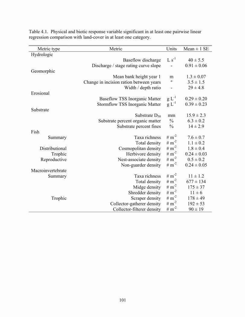
Table 4.1. Physical and biotic response variable significant in at least one pairwise linear regression comparison with land-cover in at least one category.

Metric type Metric Units Mean ± 1 SE Hydrologic

Baseflow discharge L s-1 40 ± 5.5 Discharge / stage rating curve slope - 0.91 ± 0.06

Geomorphic Mean bank height year 1 m 1.3 ± 0.07 Change in incision ration between years º 3.5 ± 1.5 Width / depth ratio - 29 ± 4.8

Erosional Baseflow TSS Inorganic Matter g L-1 0.29 ± 0.20 Stormflow TSS Inorganic Matter g L-1 0.39 ± 0.23

Substrate Substrate D50 mm 15.9 ± 2.3 Substrate percent organic matter % 6.3 ± 0.2 Substrate percent fines % 14 ± 2.9

Fish Summary Taxa richness # m-2 7.6 ± 0.7

Total density # m-2 1.1 ± 0.2 Distributional Cosmopolitan density # m-2 1.8 ± 0.4

Trophic Herbivore density # m-2 0.24 ± 0.03 Reproductive Nest-associate density # m-2 0.5 ± 0.2

Non-guarder density # m-2 0.24 ± 0.05 Macroinvertebrate

Summary Taxa richness # m-2 11 ± 1.2 Total density # m-2 677 ± 134 Midge density # m-2 175 ± 37 Shredder density # m-2 11 ± 6

Trophic Scraper density # m-2 178 ± 49 Collector-gatherer density # m-2 192 ± 53

Collector-filterer density # m-2 90 ± 19

101

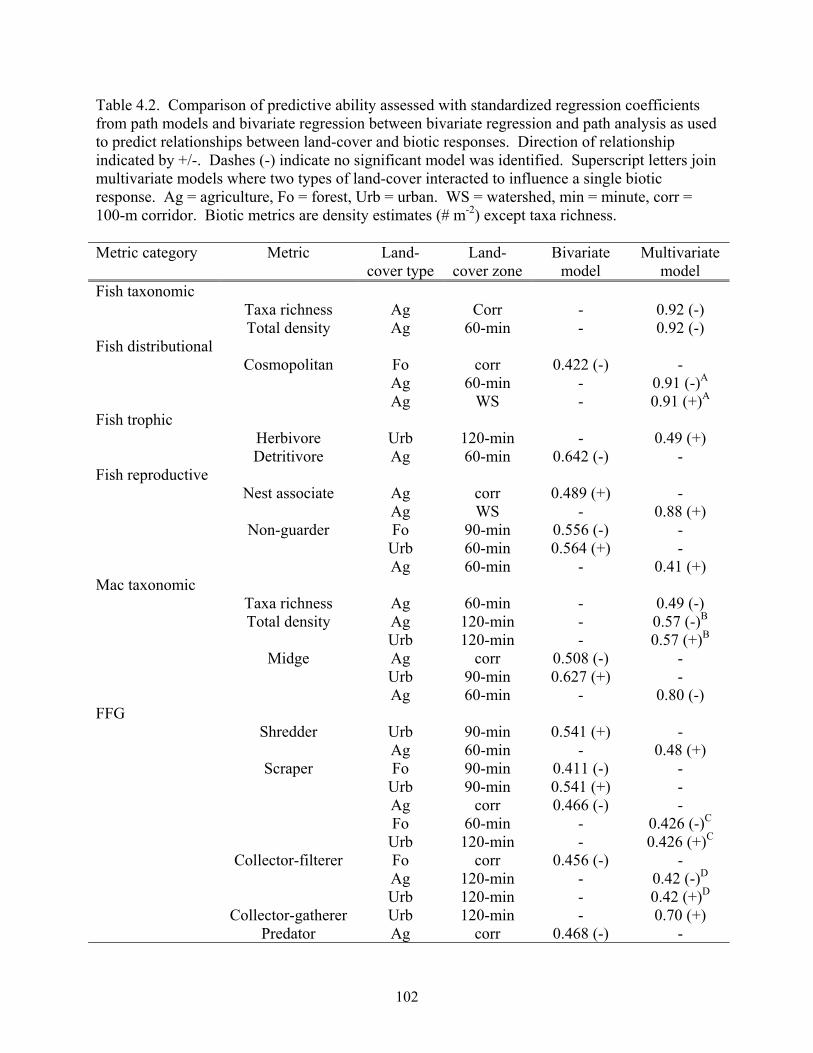
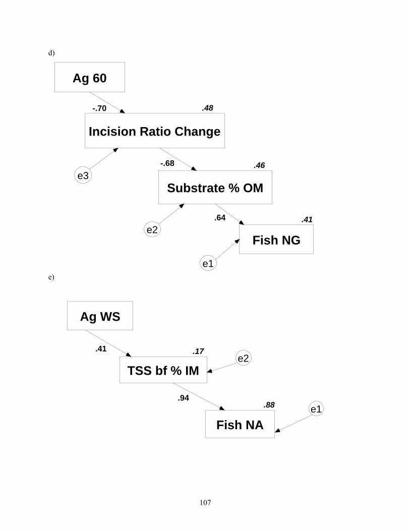
Table 4.2. Comparison of predictive ability assessed with standardized regression coefficients from path models and bivariate regression between bivariate regression and path analysis as used to predict relationships between land-cover and biotic responses. Direction of relationship indicated by +/-. Dashes (-) indicate no significant model was identified. Superscript letters join multivariate models where two types of land-cover interacted to influence a single biotic response. Ag = agriculture, Fo = forest, Urb = urban. WS = watershed, min = minute, corr = 100-m corridor. Biotic metrics are density estimates (# m-2) except taxa richness. Metric category Metric Land-

cover type Land-

cover zone Bivariate

model Multivariate

model Fish taxonomic Taxa richness Ag Corr - 0.92 (-) Total density Ag 60-min - 0.92 (-) Fish distributional Cosmopolitan Fo corr 0.422 (-) - Ag 60-min - 0.91 (-)A

Ag WS - 0.91 (+)A

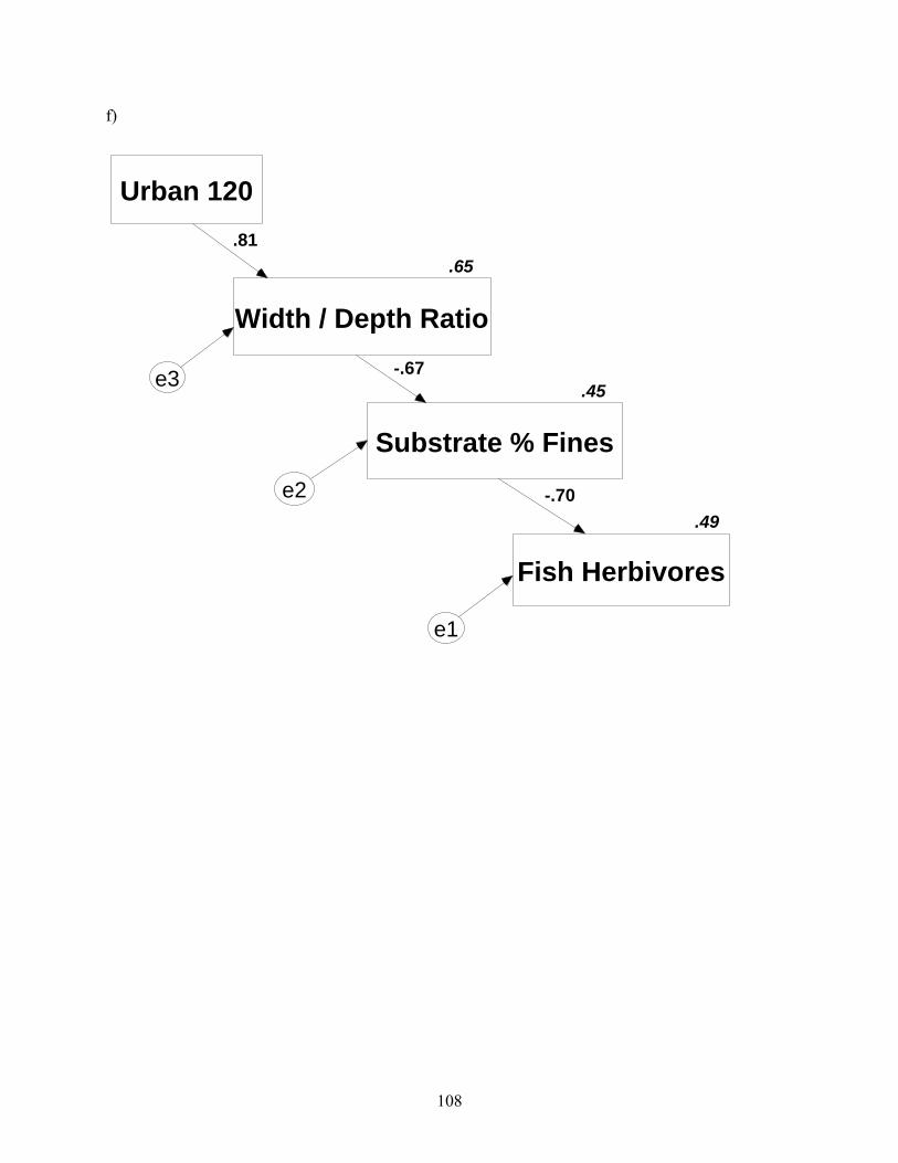
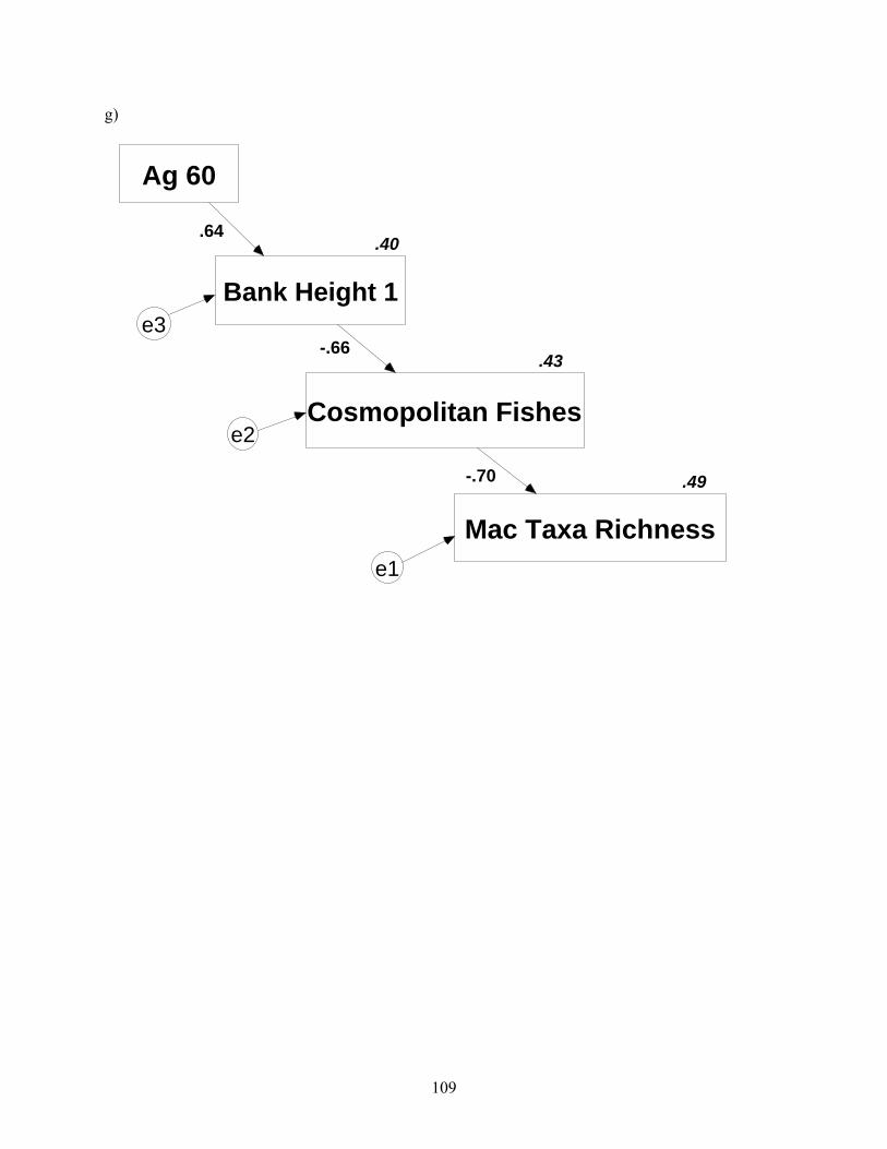
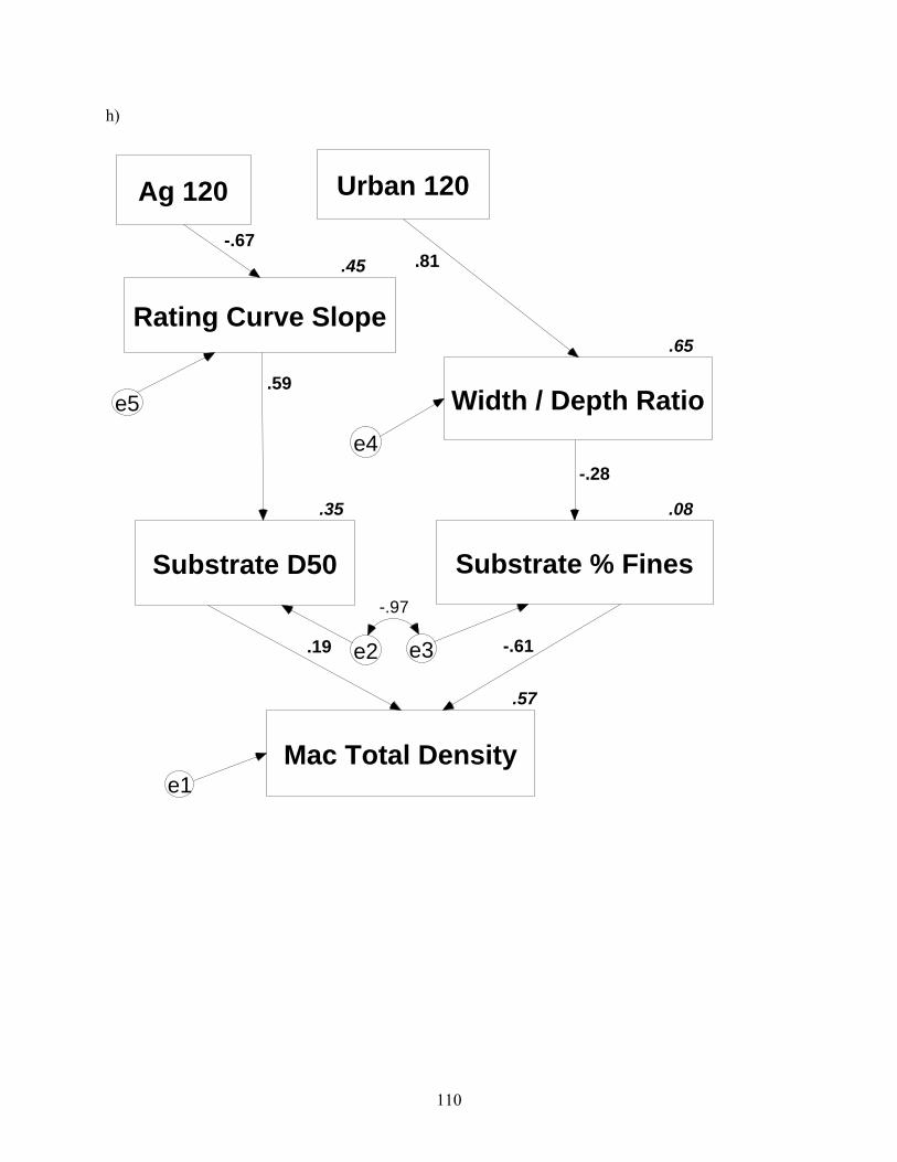
Fish trophic Herbivore Urb 120-min - 0.49 (+) Detritivore Ag 60-min 0.642 (-) - Fish reproductive Nest associate Ag corr 0.489 (+) - Ag WS - 0.88 (+) Non-guarder Fo 90-min 0.556 (-) - Urb 60-min 0.564 (+) - Ag 60-min - 0.41 (+) Mac taxonomic Taxa richness Ag 60-min - 0.49 (-) Total density Ag 120-min - 0.57 (-)B

Urb 120-min - 0.57 (+)B

Midge Ag corr 0.508 (-) - Urb 90-min 0.627 (+) - Ag 60-min - 0.80 (-) FFG Shredder Urb 90-min 0.541 (+) - Ag 60-min - 0.48 (+) Scraper Fo 90-min 0.411 (-) - Urb 90-min 0.541 (+) - Ag corr 0.466 (-) - Fo 60-min - 0.426 (-)C

Urb 120-min - 0.426 (+)C

Collector-filterer Fo corr 0.456 (-) - Ag 120-min - 0.42 (-)D

Urb 120-min - 0.42 (+)D

Collector-gatherer Urb 120-min - 0.70 (+) Predator Ag corr 0.468 (-) -

102

Table 4.3. Indices of model fit explaining how well a model fit our data.

Metric type Metric Chi-squared (X2; p > 0.05) Root mean square error of approximation (RMSEA; ≤ 0.05)

Normed Fit Index (NFI; > 0.9)

Fish Taxa richness X2 = 3.597, df = 1, p = 0.058 0.537 0.805

Total density X2 = 1.204= 3,p = 0.752 0.00 0.943

Cosmopolitan X2 = 7.580= 6,p = 0.271 0.171 0.731

Non-guarders X2 = 6.236, df = 3, p = 0.101 0.346 0.724

Nest-associates X2 = 1.999, df = 1, p = 0.157 0.333 0.872

Herbivores X2 = 4.085, df = 6, p = 0.252 0.200 0.836

Macroinvertebrate Taxa richness X2 = 4.084, df = 3, p = 0.253 0.200 0.765

Total density X2 = 21.811, df = 14, p = 0.083 0.249 0.727

Shredders X2 = 5.366, df = 3, p = 0.147 0.296 0.764

Scrapers X2 = 5.635, df = 6, p = 0.465 0.00 0.840

Collector-filterers

X2 = 6.738, df = 10, p = 0.750 0.00 0.818

Collector-gatherers

X2 = 6.995, df = 3, p = 0.072 0.385 0.785

Midges X2 = 9.727, df = 6, p = 0.137 0.263 0.652

103

Agriculture, forest, and rural development

land-cover defined at different spatial scales

Hydrologicelement

Geomorphic element

Erosional element

Depositional element

Travel Time

Baseflow discharge

w/d ratio

Storm flow TSS

Storm flow Q

Bank height

Incision ratio

Baseflow TSS Bedload D50

Substrate D50

Substrate % fines

Bedload %OM

Substrate % OM

Decreasing Spatial Scale

Fish and macroinvertebrate biotic responses

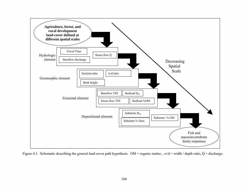
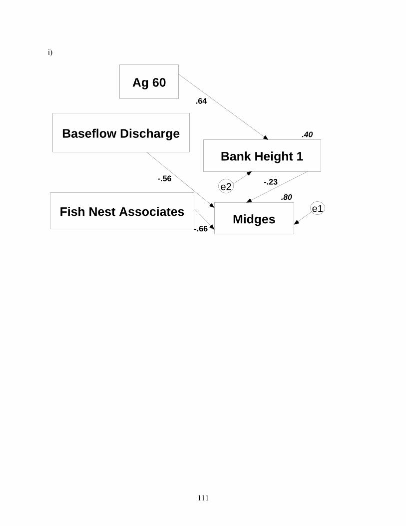
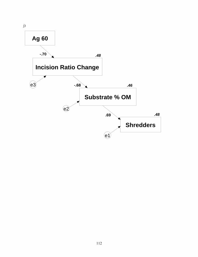
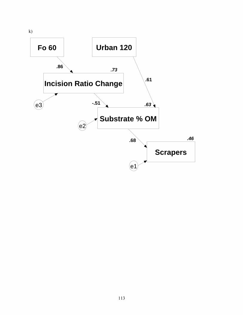
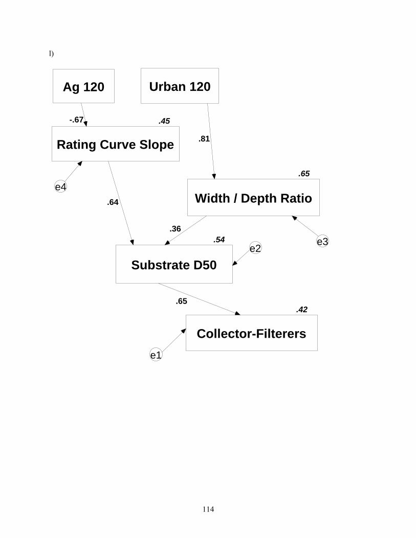
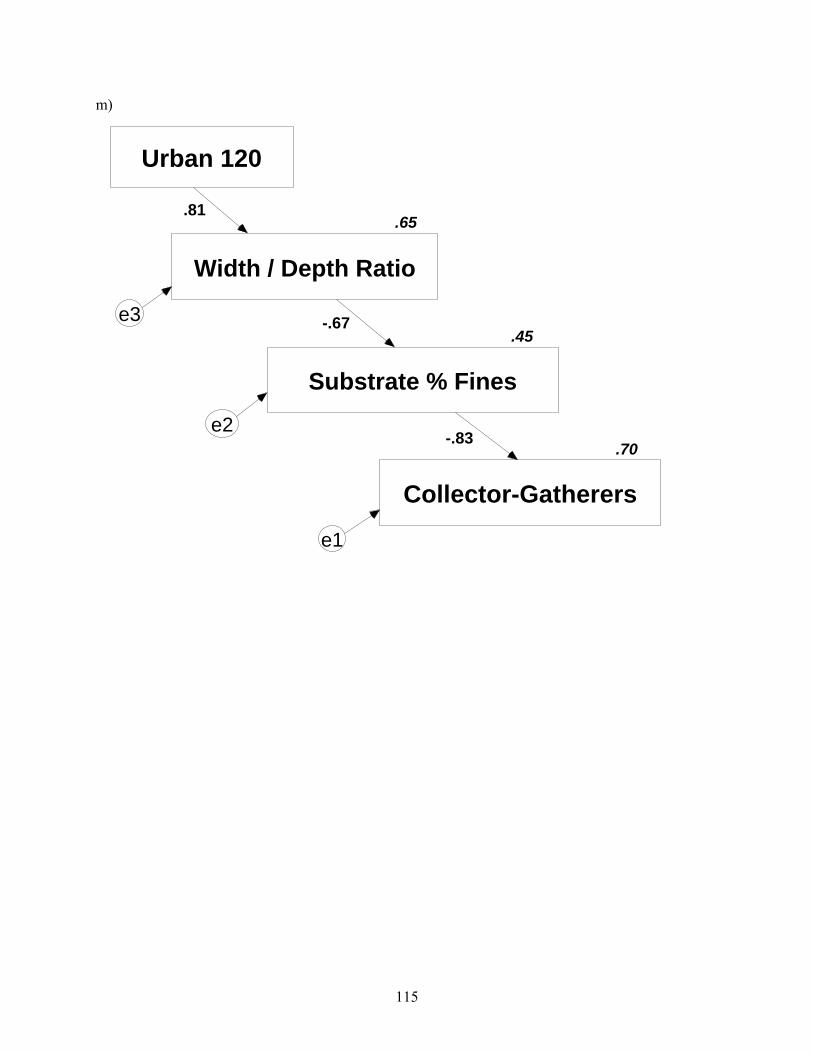
Figure 4.1. Schematic describing the general land-cover path hypothesis. OM = organic matter, , w/d = width / depth ratio, Q = discharge.

104

a)

.92

Fish TR

.06

TSS storm % IM

AG Corr

e1

e2.25

-.96

b)

.92

Fish Total Density

.40

Bank Height 1

Ag 60

e2

e1

TSS bf % IM

-.70

.64

.65

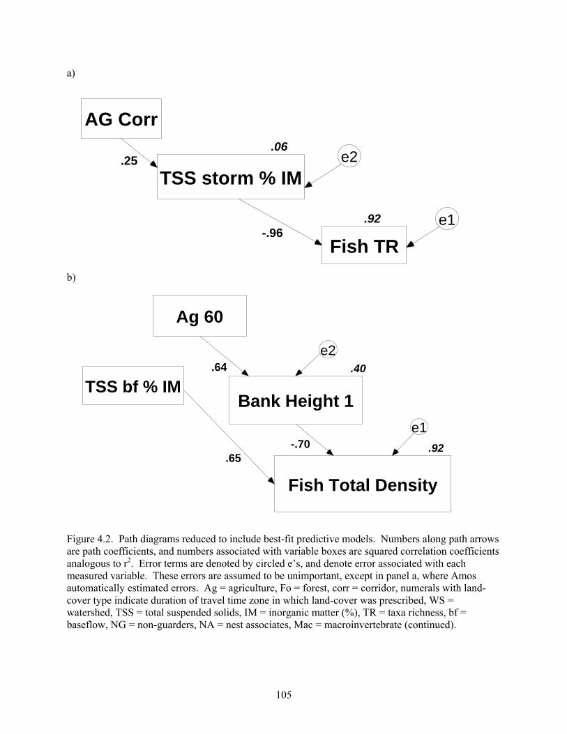
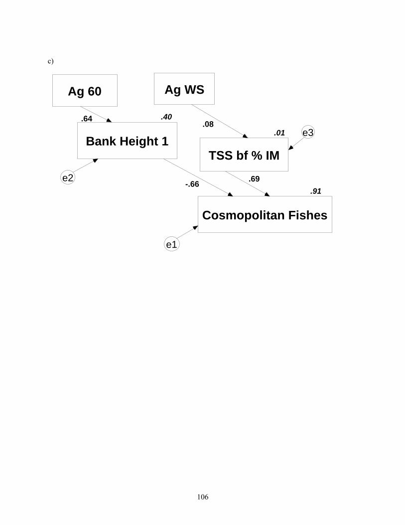
Figure 4.2. Path diagrams reduced to include best-fit predictive models. Numbers along path arrows are path coefficients, and numbers associated with variable boxes are squared correlation coefficients analogous to r2. Error terms are denoted by circled e’s, and denote error associated with each measured variable. These errors are assumed to be unimportant, except in panel a, where Amos automatically estimated errors. Ag = agriculture, Fo = forest, corr = corridor, numerals with land-cover type indicate duration of travel time zone in which land-cover was prescribed, WS = watershed, TSS = total suspended solids, IM = inorganic matter (%), TR = taxa richness, bf = baseflow, NG = non-guarders, NA = nest associates, Mac = macroinvertebrate (continued).

105

c)

.91

Cosmopolitan Fishes

.40

Bank Height 1.01

TSS bf % IM

Ag 60 Ag WS

-.66 .69e2

e3

e1

.64 .08

106

d)

.41

Fish NG

.46

Substrate % OM

.48

Incision Ratio Change

Ag 60

e3

e2

e1

-.70

-.68

.64

e)

.88

Fish NA

.17

TSS bf % IM

Ag WS

e2

e1

.41

.94

107

f)

.49

Fish Herbivores

.45

Substrate % Fines

Urban 120

e1

e2

.65

Width / Depth Ratio

e3 -.67

.81

-.70

108

g)

.40

Bank Height 1

.49

Mac Taxa Richness

e3

e1

Ag 60

.43

Cosmopolitan Fishese2

.64

-.66

-.70

109

h)

.57

Mac Total Density

Ag 120

.35

Substrate D50

.08

Substrate % Fines

.65

Width / Depth Ratio

Urban 120

.45

Rating Curve Slope

.19

e5

e4

e3e2

e1

-.67

-.97

.81

-.61

-.28

.59

110

i)

.80

Midges

.40

Bank Height 1

Ag 60

e2

e1Fish Nest Associates

Baseflow Discharge

.64

-.56 -.23

-.66

111

j)

.48

Shredders

.46

Substrate % OM

e2

e1

.48

Incision Ratio Change

Ag 60

e3

-.70

-.68

.69

112

k)

.46

Scrapers

.63

Substrate % OM

.73

Incision Ratio Change

Fo 60 Urban 120

e3

e2

e1

.61

.68

.86

-.51

113

l)

Ag 120

.45

Rating Curve Slope

Urban 120

.42

Collector-Filterers

.54

Substrate D50

.65

Width / Depth Ratio

-.67

e4

e3e2

e1

.65

.36

.81

.64

114

m)

.70

Collector-Gatherers

e1

.65

Width / Depth Ratio

Urban 120

e3.45

Substrate % Fines

e2

-.67

-.83

.81

115

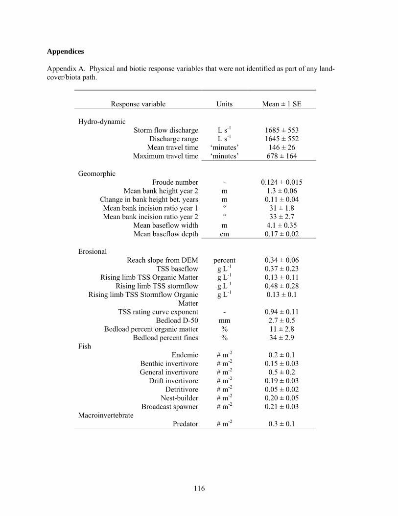
Appendices Appendix A. Physical and biotic response variables that were not identified as part of any land-cover/biota path.

Response variable

Units

Mean ± 1 SE

Hydro-dynamic

Storm flow discharge L s-1 1685 ± 553 Discharge range L s-1 1645 ± 552

Mean travel time ‘minutes’ 146 ± 26 Maximum travel time ‘minutes’ 678 ± 164

Geomorphic

Froude number - 0.124 ± 0.015 Mean bank height year 2 m 1.3 ± 0.06

Change in bank height bet. years m 0.11 ± 0.04 Mean bank incision ratio year 1 º 31 ± 1.8 Mean bank incision ratio year 2 º 33 ± 2.7

Mean baseflow width m 4.1 ± 0.35 Mean baseflow depth cm 0.17 ± 0.02

Erosional

Reach slope from DEM percent 0.34 ± 0.06 TSS baseflow g L-1 0.37 ± 0.23

Rising limb TSS Organic Matter g L-1 0.13 ± 0.11 Rising limb TSS stormflow g L-1 0.48 ± 0.28

Rising limb TSS Stormflow Organic Matter

g L-1 0.13 ± 0.1

TSS rating curve exponent - 0.94 ± 0.11 Bedload D-50 mm 2.7 ± 0.5

Bedload percent organic matter % 11 ± 2.8 Bedload percent fines % 34 ± 2.9

Fish Endemic # m-2 0.2 ± 0.1

Benthic invertivore # m-2 0.15 ± 0.03 General invertivore # m-2 0.5 ± 0.2

Drift invertivore # m-2 0.19 ± 0.03 Detritivore # m-2 0.05 ± 0.02

Nest-builder # m-2 0.20 ± 0.05 Broadcast spawner # m-2 0.21 ± 0.03

Macroinvertebrate Predator # m-2 0.3 ± 0.1

116

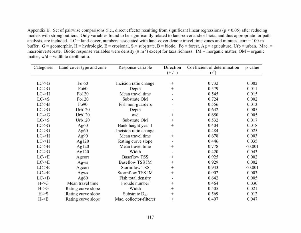
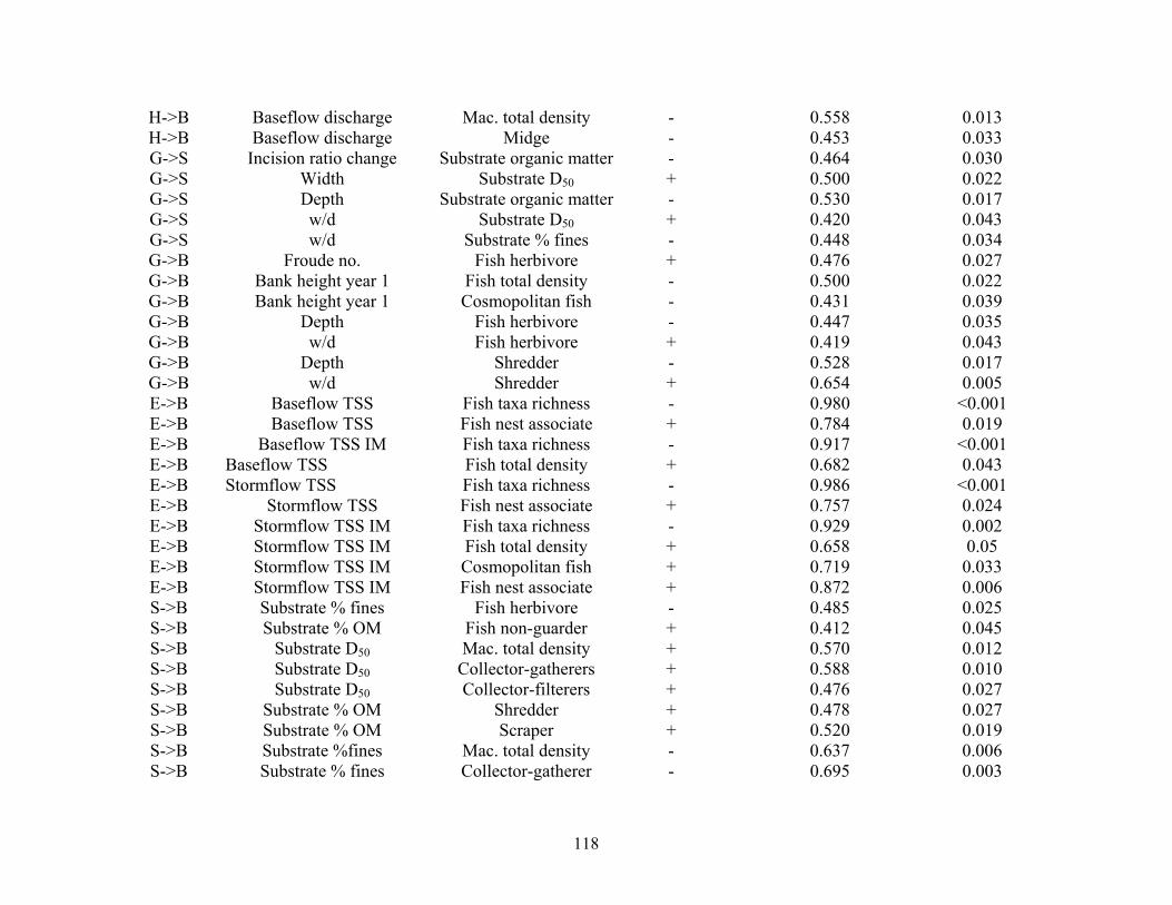
Appendix B. Set of pairwise comparisons (i.e., direct effects) resulting from significant linear regressions (p < 0.05) after reducing models with strong outliers. Only variables found to be significantly related to land-cover and/or biota, and thus appropriate for path analysis, are included. LC = land-cover, numbers associated with land-cover denote travel time zones and minutes, corr = 100-m buffer. G = geomorphic, H = hydrologic, E = erosional, S = substrate, B = biotic. Fo = forest, Ag = agriculture, Urb = urban. Mac. = macroinvertebrate. Biotic response variables were density (# m-2) except for taxa richness. IM = inorganic matter, OM = organic matter, w/d = width to depth ratio.

Categories Land-cover type and zone Response variable Direction (+ / -)

Coefficient of determination (r2)

p-value

LC->G

Fo 60

Incision ratio change

+

0.732

0.002

LC->G

Fo60 Depth + 0.579 0.011LC->H Fo120 Mean travel time - 0.545 0.015 LC->S Fo120 Substrate OM - 0.724 0.002LC->B Fo90 Fish non-guarders

- 0.556 0.013

LC->G Urb120 Depth - 0.642 0.005LC->G Urb120 w/d + 0.650 0.005LC->S Urb120 Substrate OM + 0.532 0.017LC->G Ag60 Bank height year 1 + 0.404 0.018 LC->G Ag60 Incision ratio change - 0.484 0.025 LC->H Ag90 Mean travel time + 0.678 0.003 LC->H Ag120 Rating curve slope - 0.446 0.035 LC->H Ag120 Mean travel time + 0.778 <0.001 LC->G Ag120 Width - 0.420 0.043LC->E Agcorr Baseflow TSS + 0.925 0.002LC->E Agws Baseflow TSS IM + 0.929 0.002 LC->E Agcorr Stormflow TSS + 0.943 <0.001LC->E Agws Stormflow TSS IM + 0.902 0.003 LC->B Ag60 Fish total density - 0.642 0.005 H->G Mean travel time Froude number + 0.464 0.030 H->G Rating curve slope Width + 0.505 0.021 H->S Rating curve slope Substrate D50 + 0.569 0.012H->B Rating curve slope Mac. collector-filterer + 0.407 0.047

117

H->B Baseflow discharge Mac. total density

- 0.558 0.013 H->B

Baseflow discharge Midge - 0.453 0.033G->S Incision ratio change

Substrate organic matter

- 0.464 0.030

G->S Width Substrate D50 + 0.500 0.022G->S Depth Substrate organic matter

- 0.530 0.017

G->S w/d Substrate D50 + 0.420 0.043G->S w/d Substrate % fines - 0.448 0.034 G->B Froude no. Fish herbivore + 0.476 0.027 G->B Bank height year 1 Fish total density - 0.500 0.022 G->B Bank height year 1 Cosmopolitan fish - 0.431 0.039 G->B Depth Fish herbivore - 0.447 0.035G->B w/d Fish herbivore + 0.419 0.043G->B Depth Shredder - 0.528 0.017G->B w/d Shredder + 0.654 0.005E->B Baseflow TSS Fish taxa richness - 0.980 <0.001 E->B Baseflow TSS Fish nest associate + 0.784 0.019 E->B Baseflow TSS IM Fish taxa richness - 0.917 <0.001 E->B Baseflow TSS Fish total density + 0.682 0.043 E->B Stormflow TSS Fish taxa richness - 0.986 <0.001 E->B Stormflow TSS Fish nest associate + 0.757 0.024 E->B Stormflow TSS IM Fish taxa richness - 0.929 0.002 E->B Stormflow TSS IM Fish total density + 0.658 0.05 E->B Stormflow TSS IM Cosmopolitan fish + 0.719 0.033 E->B Stormflow TSS IM Fish nest associate + 0.872 0.006 S->B Substrate % fines Fish herbivore - 0.485 0.025 S->B Substrate % OM

Fish non-guarder + 0.412 0.045

S->B Substrate D50 Mac. total density + 0.570 0.012 S->B Substrate D50 Collector-gatherers + 0.588 0.010S->B Substrate D50 Collector-filterers + 0.476 0.027S->B Substrate % OM Shredder + 0.478 0.027 S->B Substrate % OM Scraper + 0.520 0.019 S->B Substrate %fines Mac. total density - 0.637 0.006 S->B Substrate % fines Collector-gatherer - 0.695 0.003

118

B->B Cosmopolitan fish Mac. taxa richness - 0.490 0.024 B->B Nest associates Midge - 0.405 0.048

119

Chapter 5: Synthesis

Plant a new Truffula. Treat it with care. Give it clean water. And feed it fresh air. Grow a forest. Protect it from axes that hack. Then the Lorax and all of his friends may come back. – Theodor Seuss Geisel in The Lorax.

My dissertation focused on contemporary issues of stream ecology and continues the

legacy of the Virginia Tech Stream Team. Specifically, I was interested in expanding our

knowledge of how land-cover disturbance influences streams at the ecosystem scale.

Anthropogenic land-use is one of the most detrimental disturbances affecting streams worldwide

(Ramankutty et al. 2002), and a central tenet of my dissertation was determining whether rural

development influenced streams. Inherent in my approach to stream ecosystems is my use of

watersheds as organizational systems appropriate for studying streams. Researchers interested in

stream reach-scale responses (e.g., macroinvertebrate communities, nutrient spiraling, habitat

sedimentation) are currently focusing on watershed-scale phenomena that potentially influence

the responses we measure. Aquatic ecologists are still learning how to study streams at the

watershed scale, which variables are important, and what the mechanisms are that inhibit or

induce disturbance effects from the landscape to stream responses.

Linking disturbance effects to stream responses is greatly complicated by spatial scale.

Currently, research addressing how to consider the relationship between land-use spatial scale

and biotic responses is in the pioneer stages. My dissertation contributes to the spatial scale

issue by using travel time to subdivide watersheds along a spatial continuum. I designed a

method for delimiting watersheds into ecologically relevant sub-portions that could be used as

spatially explicit zones of influence to describe land-cover at multiple spatial scales. In the last

five years researchers have introduced several methods for considering landscape influence, but

travel time zones (TTZs) are the first I am aware of that use ecologically relevant criteria in their

design. TTZs helped subdivide watershed land-cover by hydrologic connectivity that I believe

represents potential areas of terrestrial-aquatic interaction. Differential land-cover influence to

stream biota associated with TTZs reflected differences in proximity and the level of potential

interaction appropriate to each biotic response. TTZs are a step toward integrating ecological

120

meaning and management objectives. Identification of critical areas of terrestrial-aquatic

interaction or potential influence could greatly enhance research, conservation, and management.

Rural development had a subtle influence on biotic assemblages and appeared to induce

changes to watershed hydrology and erosion dynamics. This relatively recent phenomenon has

not yet been well studied and my findings that rural development subtly influenced biodiversity

in streams already impaired by agriculture will contribute to our understanding of stream

disturbance response. Rural development effects were not strong enough to be detectable with

inferential statistics, but distinct biotic assemblages were present in developing and agricultural

streams. The influence of rural development appeared to be related to reduced inorganic

sediment input that was likely associated with changes to watershed hydrology. I identified

suspended solids associated with watershed hydrology and substrate as potential intermediate

links influencing biota and being influenced by land-cover.

The Land Cover Cascade design linked large-scale disturbance influence to smaller scale

biotic responses through intermediate abiotic variables that helped propagate the land-cover

disturbance. Since at least the 1970’s researchers have investigated how humans influence

streams and I have identified many of the potential cause-effect relationships involved in the

propagation of land-cover disturbance. My conclusions were mostly supportive of former

findings but unlike past studies I was able to quantify links between land-cover and biota through

known intermediate abiotic variables. Using structural equation modeling I also identified some

of the intermediate variables linking land-cover to biotic responses that traditional bivariate

techniques could not. To manage, conserve, and restore aquatic systems we must identify the

mechanisms that propagate or inhibit disturbance from influencing streams. The Land Cover

Cascade design brings us closer to identifying these mechanisms and will influence the way we

study streams in the future.

To understand relationships between humans and streams, researchers must consider

large-scale, multivariate, integrative approaches to science. I have attempted to assemble our

current knowledge of landscape/stream relationships with emerging techniques to attain a

thorough analysis of land-cover influence to stream biota. Humans continue to alter our

influence to the landscape and researchers must likewise continue to alter their approaches to

science. Combining the scientific method, past research, and creativity will bring us closer to

successful coexistence between natural systems and human needs.

121

Literature Cited

Geisel, Theodor Seuss. 1971. The Lorax. Random House, New York.

Harding, J.S., Young, R.G., Hayes, J.W., Shearer, K.A. and J.D. Stark. 1999. Changes in

agricultural intensity and river health along a river continuum. Freshwater Biology

42:345-357.

Ramankutty, N., Foley, J.A., and N.J. Olejniczak. 2002. People on the land: changes in global

population and croplands during the 20th century. Ambio 31:251-257.

122