Working Paper No. E2019/05 DCC- and DECO-HEAVY: MULTIVARIATE GARCH MODELS BASED ON REALIZED VARIANCES AND CORRELATIONS Luc Bauwens and Yongdeng Xu February 2019 (Revised August 2021) ISSN 1749-6010 Cardiff Economics Working Papers This working paper is produced for discussion purpose only. These working papers are expected to be published in due course, in revised form, and should not be quoted or cited without the author’s written permission. Cardiff Economics Working Papers are available online from: http://econpapers.repec.org/paper/cdfwpaper/ and business.cardiff.ac.uk/research/academic-sections/economics/working-papers Enquiries: [email protected]Cardiff Business School Cardiff University Colum Drive Cardiff CF10 3EU United Kingdom t: +44 (0)29 2087 4000 f: +44 (0)29 2087 4419 business.cardiff.ac.uk
Transcript
Working Paper No. E2019/05
DCC- and DECO-HEAVY: MULTIVARIATE
GARCH MODELS BASED ON REALIZED
VARIANCES AND CORRELATIONS
Luc Bauwens and Yongdeng Xu
February 2019
(Revised August 2021)
ISSN 1749-6010
Cardiff Economics Working Papers
This working paper is produced for discussion purpose only. These working papers are expected to be published in
due course, in revised form, and should not be quoted or cited without the author’s written permission.
Cardiff Economics Working Papers are available online from:
This paper introduces the scalar DCC-HEAVY and DECO-HEAVY modelsfor conditional variances and correlations of daily returns based on measuresof realized variances and correlations built from intraday data. Formulas formulti-step forecasts of conditional variances and correlations are provided.Asymmetric versions of the models are developed. An empirical study showsthat in terms of forecasts the new HEAVY models outperform the BEKK-HEAVY model based on realized covariances, and the BEKK, DCC andDECO multivariate GARCH models based exclusively on daily data.
The covariance matrix of daily asset returns is used in several applications of financialmanagement. Therefore, modeling the temporal dependence in the elements ofthe covariance matrix, often with the ultimate aim of forecasting, is a key area offinancial econometrics. The most widespread model class for this purpose is that ofmultivariate generalized autoregressive conditional heteroscedasticity (MGARCH)models, wherein the conditional covariance matrix of daily returns is specified asa deterministic function of past daily returns. A survey of MGARCH models isprovided by Bauwens et al. (2006).
The increasing availability of intraday data has led to the development of so-called “High-frEquency-bAsed VolatilitY”(HEAVY) models, initially in the univari-ate case (Engle and Gallo, 2006; Shephard and Sheppard, 2010). In the multivariatecase, such models have been introduced in the stochastic volatility framework byJin and Maheu (2013), and in the MGARCH one by Noureldin et al. (2012). In thelatter framework, the main difference is that the conditional covariance matrix ofdaily returns is specified in the HEAVY case as a function of lagged realized covari-ances, instead of lagged outer products of daily returns in the traditional MGARCHcase. Thus, multi-step forecasts of daily conditional covariance matrices by HEAVYmodels require as input forecasts of realized covariances, which are obtained froma dynamic model for the realized covariance matrix. HEAVY models are based onmore accurate measurements of covariances than GARCH models, and they im-prove forecasts of the conditional covariance matrix of daily returns, as illustratedby Noureldin et al. (2012). A different class of models that relate the daily returnvolatility to a realized volatility measure is the realized GARCH model of Hansenet al. (2012); this type of model has been extended to the multivariate setup byHansen et al. (2014) and Gorgi et al. (2019).
A well-known difficulty of MGARCH and HEAVY models is that the number ofparameters they require tends to be large, being at least a quadratic function of thedimension of the return vector. Therefore, when the dimension is more than a hand-ful of assets, a scalar parameterization is adopted. For example, Noureldin et al.(2012), for ten assets, and Opschoor et al. (2018), for thirty assets, adopt the scalarBEKK parameterization (see Engle and Kroner, 1995). This parameterization, cou-pled with a targeting procedure, which is a way to estimate the constant parametermatrices of the model, facilitates the estimation of the remaining scalar parametersenormously, since their number is independent of the dimension. The scalar BEKKparameterization implies that the conditional variances and covariances have thesame persistence and the same sensitivity to the past realized covariances, whichmay be unrealistic for a large number of assets. A Factor-HEAVY model, proposedby Sheppard and Xu (2019), avoids this drawback of the scalar BEKK while keepingthe number of parameters manageable for estimation.
2
The first contribution of this research is the extension of the HEAVY class bythe DCC (Engle, 2002) and DECO (Engle and Kelly, 2012) specifications. ScalarDCC-HEAVY and DECO-HEAVY models are developed. Like it was done for theBEKK-HEAVY, these models use well-known formulations of the correspondingMGARCH models, modifying them by specifying the dynamics of the daily condi-tional correlation matrix as a function of past realized correlations. Likewise, themodel we propose for the realized correlation matrix is of DCC-type, instead ofBEKK-type. In both parts of the model, there is a decoupling of the parametersof the variance dynamics (daily or realized) from those of the model for the corre-sponding correlation matrix. The decoupling has been shown to be advantageousin several respects for MGARCH models: the scalar DCC is a more flexible modelthan the scalar BEKK and usually provides a better empirical fit even after takinginto account its heavier parameterization; each part of the model can be estimatedby QML in two steps (one for the variance equations, one for the correlation) whichmakes it practical for handling a dimension of more than a handful of assets; andit usually improves the forecast quality. The same advantages occur in the scalarHEAVY model context, and this is confirmed empirically.
The proposed DCC-HEAVY formulation is different from the model of Braione(2016), where the dynamics of the daily correlation matrix is driven by the outerproduct of the past degarched returns (which is not a correlation matrix), while themodel for the realized covariances and variances is of BEKK-type. An advantageof the new specifications is that they allow us to forecast directly the correlationsseveral steps ahead, avoiding an approximation due to the fact that otherwise, cor-relations are obtained by normalizing quasi-correlations.
Stationarity conditions and formulas for multi-step forecasts are derived froma vector multiplicative error representation of the DCC-HEAVY model where thedynamics is driven both by lagged realized measures and outer products of pastdegarched returns, thus encompassing both DCC-HEAVY and DCC-GARCH. Fur-thermore, asymmetric impact and HAR-type terms (Corsi, 2009) are added to theDCC- and DECO-HEAVY models.
The second contribution of this research is a detailed empirical comparison ofthe BEKK, DCC and DECO HEAVY and GARCH models. All models are appliedto the stocks in the Dow Jones Industrial Average (DJIA) index. Like in Shep-hard and Sheppard (2010), the effects of the lagged squared returns are insignificantwhen lagged realized variances are included in the conditional variance equations.Likewise, the effect of the lagged outer product of degarched returns is insignificantwhen the lagged realized correlation matrix is included in the conditional corre-lation equation. Moreover, applying the model confidence set approach based onstatistical and economic loss functions, the empirical results show that the DCC-and DECO-HEAVY models provide better out-of-sample forecasts than the DCC-GARCH, DECO-GARCH, BEKK-GARCH, and BEKK-HEAVY models. Including
3
asymmetric and HAR terms further improve the DCC- and DECO-HEAVY modelforecasts.
The remainder of the paper is organized as follows. Section 2 introduces theDCC- and DECO-HEAVY models. Section 3 provides the multiplicative error repre-sentation, the multi-step forecast formulas, and model extensions. Section 4 presentsthe estimation procedure. Section 5 provides the empirical results. Section 6 con-cludes. A supplementary appendix (SA) includes additional theoretical and empir-ical results, in particular for a dataset used by Noureldin et al. (2012).
2 DCC-HEAVY and DCC-DECO Models
In the first subsection, the multivariate HEAVY framework of Noureldin et al. (2012)is reminded, and in particular the scalar BEKK-HEAVY model. The scalar DCC-HEAVY and DCC-DECO models are defined in the next subsections.
2.1 Multivariate HEAVY Framework
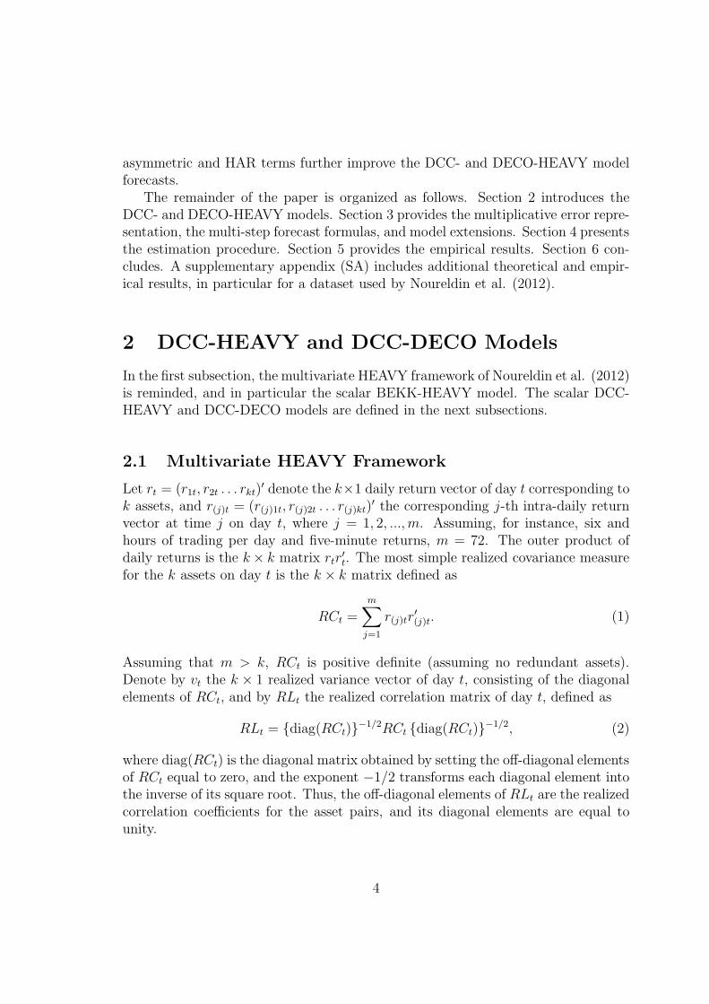
Let rt = (r1t, r2t . . . rkt)′ denote the k×1 daily return vector of day t corresponding to
k assets, and r(j)t = (r(j)1t, r(j)2t . . . r(j)kt)′ the corresponding j-th intra-daily return
vector at time j on day t, where j = 1, 2, ..., m. Assuming, for instance, six andhours of trading per day and five-minute returns, m = 72. The outer product ofdaily returns is the k× k matrix rtr
′t. The most simple realized covariance measure
for the k assets on day t is the k × k matrix defined as
RCt =
m∑
j=1
r(j)tr′(j)t. (1)
Assuming that m > k, RCt is positive definite (assuming no redundant assets).Denote by vt the k × 1 realized variance vector of day t, consisting of the diagonalelements of RCt, and by RLt the realized correlation matrix of day t, defined as
RLt = diag(RCt)−1/2RCt diag(RCt)
−1/2, (2)
where diag(RCt) is the diagonal matrix obtained by setting the off-diagonal elementsof RCt equal to zero, and the exponent −1/2 transforms each diagonal element intothe inverse of its square root. Thus, the off-diagonal elements of RLt are the realizedcorrelation coefficients for the asset pairs, and its diagonal elements are equal tounity.
4
A multivariate HEAVY model specifies a dynamic process for the conditionalcovariance matrix Ht of the daily return and another one for the conditional meanMt of the realized covariance matrix of day t:
E(rtr′t|Ft−1) := Ht, (3)
E(RCt|Ft−1) := Mt, (4)
where Ft−1 is the information set generated by the daily and intra-daily observations,and E(rt|Ft−1) = 0 is assumed for simplicity (otherwise rt denotes the demeanedreturn vector). The link between both moments comes from the dependence of Ht
on past values of functions of RCt.For the specification of the dynamics of Ht andMt, Noureldin et al. (2012) adopt
the BEKK-type model to ensure that the conditional covariance matrix is positivesemidefinite. The scalar version of the model, with the ‘targeting’ parameterizationof the constant terms, is
Ht = (1− βH)H − αHM + αHRCt−1 + βHHt−1, (5)
Mt = (1− αM − βM)M + αMRCt−1 + βMMt−1, (6)
where the k× k matrices H = E(rtr′t) and M = E(RCt) are assumed to be positive
definite (PD), and targeting means that these matrices are replaced by their em-pirical counterparts. For (6), sufficient restrictions for the positivity of Mt are thatαM ≥ 0, βM ≥ 0, βM = 0 if αM = 0, and αM + βM < 1. For (5), the restrictionsαH ≥ 0, βH ≥ 0, βH = 0 if αH = 0, βH < 1 are not sufficient to ensure that(1 − βH)H − αHM , hence Ht, be positive definite. The issue is explained in detailin Section A of the SA, where the equivalence between (5) and one of the covariancetargeting parameterizations of Noureldin et al. (2012) is shown. For estimation, inpractice we check that Ht (rather than (1−βH)H−αHM) is positive definite in thesample period during the numerical maximizing of the log-likelihood function, butfor both datasets we use, no lack of PDness occurred.
The scalar BEKK-GARCH model corresponds to the equation (5) for Ht above,where RCt−1 is replaced by rt−1r
′t−1 and M by H, thus using only the daily infor-
mation.
2.2 DCC-HEAVY Model
An alternative to the BEKK specification for Ht and Mt is the DCC model of Engle(2002). Any covariance matrix can be written as the product DRD, where D isthe corresponding diagonal matrix of standard deviations and R is the correlationmatrix.
5
2.2.1 DCC-HEAVY Specification of Ht
Let us denote by ht the k × 1 vector of conditional variances (that is, the diagonal
elements of Ht), by h1/2t the vector of conditional standard deviations (obtained by
taking the square root of each entry of ht), and by Rt the corresponding conditionalcorrelation matrix. Then, the conditional covariance matrix, Ht can be written as
Ht = Diag(h1/2t )Rt Diag(h
1/2t ), (7)
where, for x being a k × 1 vector, Diag(x) is the k × k diagonal matrix with theentries of x as diagonal elements.
Assumption (3) for the HEAVY-BEKK is replaced by
E(diag(rtr′t)|Ft−1) := Diag(ht), (8)
E(utu′t|Ft−1) := Rt, where ut = rt ⊙ h
−1/2t . (9)
Thus, instead of specifying altogether the dynamics of the conditional variances andcovariances of the returns as for instance in (5), the DCC-HEAVY model specifiesthe dynamics of the conditional variances of the returns and of the conditionalcorrelation matrix (Rt) of the degarched returns (i.e. the observed returns dividedby their conditional standard deviations). Notice indeed that
E(utu′t|Ft−1) = E(rtr
′t|Ft−1)⊙
(
h−1/2t (h
−1/2t )′
)
= Ht ⊙(
h−1/2t (h
−1/2t )′
)
is a matrix with unit diagonal elements, and off-diagonal elements that are theconditional correlation coefficients, that is, the conditional covariances divided bythe corresponding conditional standard deviations. This is the same setting as inthe DCC-GARCH model of Engle (2002), and since a covariance is the productof two standard deviations and a correlation, the expectation of the covariance isnot the corresponding function of the expected standard deviations and expectedcorrelation.
The dynamics of the conditional variance vector is specified as
ht = ωh + Ahvt−1 +Bhht−1, (10)
where ωh is a k×1 positive vector, and Ah and Bh are k×k matrices, such that eachentry of ht is positive. To ease the restrictions necessary for this and to avoid pa-rameter proliferation, Ah and Bh are restricted to be diagonal matrices with positiveentries on the diagonal, and the elements on the diagonal of Bh to be smaller thanunity. The diagonality restrictions imply that each conditional variance depends onits own lag and the corresponding previous realized variance, as in the HEAVY-rmodel of Shephard and Sheppard (2010). More generally, Ah can be non-diagonal to
6
allow spillover effects. If Bh is restricted to be diagonal, the model of the k variancescan be estimated in k separate parts (see Section 4). The DCC-GARCH model ofEngle (2002) for the conditional variances is similar to (10), with r2t−1 (the squaredelements of rt−1) replacing vt−1.
The conditional correlation matrix is specified through a scalar dynamic equa-tion:
Rt = R + αrRLt−1 + βrRt−1, (11)
R = (1− βr)R− αrP , (12)
where αr ≥ 0, βr ≥ 0, βr = 0 if αr = 0, βr < 1, R is the k × k unconditionalcorrelation matrix of ut, and P is the k × k unconditional expectation of RLt.The elements of R and P can be set to their empirical counterpart to simplify theestimation, so that only two parameters (αr and βr) remain to be estimated. Bysubstituting (12) in (11), Rt is equal to R + αr(RLt−1 − P ) + βr(Rt−1 − R), andby taking the unconditional expectation on both sides, E(Rt) = R if E(RLt) = P .The specification of Rt is similar in spirit to the specification of Ht in (5),by takinginto account that E(Rt) is not equal to E(RLt), like E(RCt) 6= E(Ht).
Since R, P and RLt−1 have unit diagonal elements, and assuming that the initialmatrix R0 is a correlation matrix, it is obvious that Rt has unit diagonal elements,but to be a well-defined correlation matrix it must be positive definite (PD). Thisis not necessarily the case for the set of values of (αr, βr) stated above. The issue isillustrated in Section B of the SA. For estimation, we proceed (like for the BEKK-HEAVY model) by checking that Rt (rather than R) is positive definite in the sampleperiod during the numerical maximizing of the log-likelihood function. Like for theBEKK-HEAVY model, for the datasets we use, no issue of lack of PDness occurred.
An advantage of the proposed specifications of Rt, based on the realized corre-lation matrix, is that there is no need to transform the covariance matrix of thedegarched returns into a correlation one, as in the DCC-GARCH model of Engle(2002), which is specified by
Rt = diag(Qt)−1/2Qtdiag(Qt)
−1/2, (13)
with the k × k symmetric PD matrix
Qt = (1− αq − βq)Q+ αqut−1u′t−1 + βqQt−1, (14)
where αq ≥ 0, βq ≥ 0, βq = 0 if αq = 0, αq +βq < 1, and Q is a k×k PD matrix. Qt
is actually the conditional covariance matrix of ut, with non-unit diagonal elements,and by (13), it is transformed into a correlation matrix. However, this parameteri-sation raises two issues, one about estimation, the other about forecasting.
First, because E(utu′t|Ft−1) = Rt 6= Qt, Q is not equal to E(Qt) and therefore is
not consistently estimated by∑
t utu′t/T . Thus using this average to estimate Q as
7
proposed by Engle (2002), so that only αq and βq remain to be estimated by QML,introduces an asymptotic bias in their estimator. See Aielli (2013) for details andan alternative formulation of (14) that avoids this problem.
Second, at date t, the (s+1)-step ahead forecast ofRt+s+1 requires Et(ut+su′t+s) =
Et(Rt+s), which is not available in closed from due to the nonlinear relation (13)between Rt+s and Qt+s. By assuming Et(Rt+s) ≈ Et(Qt+s), Engle and Sheppard(2001) obtain the closed form forecast recurrence relation
Et(Rt+s+1) = Q+ (αq + βq)Et(Rt+s − Q) (15)
that starts with Et(Rt+1) = Rt. The correlation forecasts are thus approximate andbiased.
The DCC-HEAVY model differs from DCC-GARCH model in three ways: 1)the dynamics of conditional variances ht are driven by the lagged realized volatilitiesvt−1; 2) the conditional correlation Rt is modelled directly rather than parameterisedin a sandwich form as in (13); 3) the dynamics of the conditional correlation matrixRt are driven by the lagged realized correlation matrix. The last two features allowus to obtain exact closed forms for s-step ahead correlation forecasts, as explainedin Section 3.
2.2.2 DCC-HEAVY Specification of Mt
The specification of the DCC-HEAVY model requires to define the dynamics of
Mt = Diag(m1/2t )PtDiag(m
1/2t ), (16)
where mt is the vector containing the main diagonal of Mt, that is, the conditionalmeans of the realized variances, and Pt is the corresponding conditional mean of therealized correlation matrix.
The conditional expectation of the realized variances is specified as
mt = ωm + Amvt−1 +Bmmt−1, (17)
where ωm is a positive k×1 vector, Am and Bm are k×k matrices that are restrictedto be diagonal matrices with positive entries, as discussed after (10).
The dynamic process for the conditional expectation of the realized correlationmatrix is defined in the following way:
Pt = (1− αp − βp)P + αpRLt−1 + βpPt−1, (18)
where αp ≥ 0, βp ≥ 0, βp = 0 if αp = 0, αp + βp < 1, and P is a correlationmatrix that is the unconditional mean of RLt. The elements of P can be set to
8
their empirical counterpart to render the estimation simpler. E(RLt) is not equalto the unconditional correlation matrix E(Pt), due to the nonlinearity of the thetransformation from covariance to correlation. However, Bauwens et al. (2012) showthat if RCt is computed from a large enough number of high-frequency returns, Pshould be almost equal to E(RLt).
Equations (7)-(18) form the DCC-HEAVY model. By setting αr = βr = αp =βp = 0, the model simplifies into a constant conditional correlation HEAVY model.Estimation is discussed in Section 4.
2.3 DECO-HEAVY Model
The DECO-HEAVY model differs from the DCC-HEAVY in the specification of theconditional correlation matrix corresponding to Ht and of the conditional mean ofthe realized correlation matrix corresponding to Mt.
The specification of the conditional correlation matrix corresponding to Ht, de-noted by RE
t , is based on the assumption that all the conditional correlations arethe same time-varying correlation ρt ∈ (−1/(k − 1), 1), chosen to be the average ofthe correlation coefficients of Rt = (rt,ij), defined by (11)-(12):
REt = (1− ρEt )Ik + ρEt Jk, (19)
ρEt =2
k(k − 1)
∑
i>j
rt,ij. (20)
where Jk is k × k matrix of ones. The DECO-GARCH model of Engle and Kelly(2012) is using as dynamic equicorrelation coefficient the average of the DCC-GARCH correlations defined by (13) together with the modification of (14) proposedby Aielli (2013).
Likewise, the conditional mean of the realized correlation matrix correspondingto Mt, denoted by PE
t , is specified as:
PEt = (1− ρPt )Ik + ρPt Jk, (21)
ρPt =2
k(k − 1)
∑
i>j
pt,ij . (22)
The main advantage of DECO with respect to DCC, especially when k is verylarge, is the availability of analytical expressions of the inverse and determinant ofthe equicorrelated matrices, which are used in the computation of the likelihoodfunction for estimation, and of economic loss functions for forecast evaluations. Formore details, see Engle and Kelly (2012).
9
3 Representation, Forecasting and Extensions
In this section, the DCC-HEAVY and the closely related DCC-GARCH, and DCCX-GARCHX models are represented as multiplicative error models (MEM), from whichstationarity conditions and closed-form formulas for multi-step forecasts follow di-rectly. An extension of the the DCC-HEAVY model is proposed by adding asym-metric impact and HAR terms.
3.1 Multiplicative Error Representation
A MEM for a positive variable xt specifies it as the product of a positive conditionalmean and a positive error that follows some distribution with expectation equalto one. If xt is a squared centred return, the conditional mean is the conditionalvariance. This can be extended to the elements of a vector. In this subsection, thefocus is on the conditional expectation formulation, not on the distribution.
For the conditional and realized variance equations, define the vectors of 2k × 1elements xt = [(r2t )
′, v′t]′ and µt = [h′
t, m′t]′. The conditional expectation formulation
of the conditional and realized variance equations (10) and (17) is
E(xt|Ft−1) := µt,
µt = ω + Axt−1 +Bµt−1, (23)
where
ω=
[
ωh
ωm
]
, A=
[
0 Ah
0 Am
]
, B=
[
Bh 00 Bm
]
(24)
and the 0 symbol stands for a k × k matrix of zeros. If
A=
[
Ah 00 Am
]
, (25)
the top part becomes the DCC-GARCH model, and the realized variance model iskept in the bottom part. If
A=
[
Ah Ahm
0 Am
]
, (26)
the model (referred to as DCC-GARCHX) includes in the top part both the laggedsquared return and the lagged realized variance, encompassing the two previousmodels.
Defining the 2k × k matrices Yt = [utu′t, RLt]
′ and Φt = [Rt, Pt]′, the conditional
expectation formulation of the conditional and realized correlation matrix equations(11) and (18) is
E(Yt|Ft−1) := Φt,
Φt = Ω + (α⊗ Jk)Yt−1 + (β ⊗ Jk)Φt−1, (27)
10
where
Ω=
[
RP
]
, α=
[
0 αr
0 αp
]
, β=
[
βr 00 βp
]
,
and the 0 symbol is scalar in this case. If α=
[
αq 00 αp
]
, β=
[
βq 00 βp
]
, Qt replaces
Rt in the definition of Φt, and the constant term is adapted, the top part becomes the‘quasi-correlation’ equation (14) of the DCC-GARCH model, the realized correlationequation being kept in the bottom part. If
α=
[
αq αr
0 αp
]
, β=
[
βr 00 βp
]
, (28)
both ut−1u′t−1 andRL′
t−1 are included in the top part (referred to as DCCX-GARCH).Processes such as defined by (23) and (27) can be written as VARMA(1,1) by
defining appropriate error terms. From this representation, it follows that the co-variance stationarity condition is that the largest eigenvalue of A + B is smallerthan unity for (23), and likewise for the largest eigenvalue of α+β for (27). For thematrices α and β defined after (27), the previous condition is equivalent to βr < 1and αp + βp < 1, as written after (11) and (18). The unconditional first momentis then obtained by applying standard results for the VARMA representations. Forexample, E(xt) = (I2k −A−B)−1ω, which gives E(vt) = (Ik −Am −Bm)
−1ωm andE(r2t ) = (Ik − Bh)
−1[ωh + AhE(vt)] for the variances of the DCC-HEAVY model.For the correlations, E(RLt) = P and E(utu
′t) = [R+αrE(RLt)]/(1− βr) = R, the
last equality resulting from (12).
3.2 Multiple-step Ahead Forecasting
Forecasts of the conditional covariance matrices of daily returns are used in severalfinancial applications. The s-step ahead forecast of Ht+s, computed at date t, isdefined in the case of DCC-type models as
Ht+s|t = Diag
[Et(ht+s)]1/2
Et(Rt+s)Diag
[Et(ht+s)]1/2
, (29)
where Et(.) is a short notation for E(.|Ft−1). Notice that as in the DCC model,Ht+s|t is not equal to Et(Ht+s), due to the nonlinearity of the transformation ofcovariances into correlations and of the square root function.
To obtain Et(ht+s) and Et(Rt+s), the conditional expectation expressions of theprevious subsection are useful to compute Et(µt+s) and Et(Φt+s), denoted by µt+s|t
and Φt+s|t, respectively.Starting from (23) leads to Et(µt+s). In moving more than one step ahead,
xt+s|t is not known and needs to be substituted with its corresponding conditional
11
expectation µt+s|t, hence
µt+1|t = ω + Axt +Bµt,
µt+s|t = ω + (A+B)µt+s−1|t for s ≥ 2, (30)
which can be solved recursively, giving the closed form forecast
µt+s|t = ω + Cs−1µt+1|t for s ≥ 2,
where ω = (I − C)−1(I − Cs−1)ω and C = A+B.Proceeding in the same way for Et(Φt+s) from (27) gives
Φt+1|t = Ω + (α⊗ Jk)Yt + (β ⊗ Jk)Φt,
Φt+s|t = Ω + ((α + β)⊗ Jk) Φt+s−1|t for s ≥ 2. (31)
The closed form forecast is
Φt+s|t = Ω +(
cs−1 ⊗ Jk
)
Φt+1|t for s ≥ 2,
where Ω = (I − c)−1(I − cs−1)Ω and c = α + β.For instance, the DCC-HEAVY model s-step ahead forecasts µt+s|t and Φt+s|t
are derived from (30) and (31) by setting A, B, α, and β to the matrices definedafter (23) and (27). The s-step ahead forecast Et[ht+s] of the conditional variancevector corresponds to the first k elements of µt+s|t, and the s-step forecast Et[Rt+s]of the conditional correlation corresponds to the k × k upper block of Φt+s|t.
3.3 Model Extensions
It has long been discovered that stock markets react differently to positive andnegative news. The asymmetric effect is now commonly used to refer to any volatil-ity model, univariate and multivariate alike, in which the (co)variances respondasymmetrically to positive and negative shocks. The DCC-HEAVY model can beextended by incorporating the asymmetric effect into the variance and correlationequations. In the variance equation, the asymmetric effect implies that volatilitytends to increase more following negative return shocks than equally-sized positiveshocks. In the correlation equation, the asymmetric effect implies that the corre-lation between stock returns tends to increase when the market turns down. Theextended model is called ADCC-HEAVY model.
Define dt = (d1t, d2t, ..., dkt)′ where dit = 1 if rit < 0 and dit = 0, if rit ≥ 0, for
i = 1, .., k, and Dt = dtd′t − diag(dtd
′t) (a matrix with diagonal elements equal to 0).
12
The conditional variance and correlation equations of the ADCC-HEAVY model arethen
ht = ωh + Ahvt−1 +Bhht−1 + Γhdt−1 ⊙ vt−1, (32)
Rt = R + αrRLt−1 + βrRt−1 + γrDt−1 ⊙ RLt−1, (33)
R = (1− βr)R − (αrP + γrD ⊙ P ), (34)
where Γh is a k × k diagonal matrix and D is the sample mean of Dt. Equation(32) extends (10); asymmetric effects correspond to positive values on the diagonalof Γh. Equations (33)-(34) extend (11)-(12). The asymmetric effect corresponds toa positive value of γr: the impact of the lagged realized correlation between assets iand j on their current conditional correlation is equal to αr + γr only if both ri,t−1
and rj,t−1 are negative, otherwise the impact is reduced to αr if γr is positive. Noticethat the diagonal elements of Dt−1⊙RLt−1 and D⊙ P are equal to one, so that thesame holds for Rt. Like in the simpler model where γr = 0, in estimation (αr, βr, γr)are constrained to values such that Rt is PD for all t. In the empirical applications,this did not create any difficulty.
The same asymmetric effects are included in the realized variance and corre-lation equations. Furthermore, the heterogeneous autoregressive (HAR) model ofCorsi (2009) has emerged as a simple and powerful way to include the long-memoryfeature of realized volatilities. The model was extended to the multivariate settingby Chiriac and Voev (2011) and Oh and Patton (2016). Adding also HAR terms tothe realized variance and correlation equations, respectively (17) and (18), resultsin the richer dynamic equations
p −αmp )P . Although Pt has unit diagonal elements, in estimation
the parameter space must be constrained to ensure that this matrix is PD for all t.HAR terms are not added to the conditional covariance and correlation equations,since these effects are insignificant in the empirical application.
Other ways to define the asymmetric effect have been used. For example, onecan define dit = 1 when the stock volatility RCii,t is ‘high’ (above some threshold).In the correlation equation, that implies that the correlation between two stockreturns increases more when both stocks are highly volatile than if only one or noneis highly volatile. Another asymmetric effect is to let all correlations increase ifthe market volatility (for instance measured by VIX) increases, see Bauwens andOtranto (2016).
13
Section C of the SA provides the formulas of multiple step forecasts of the ex-tended models.
4 Estimation
The DCC- and DECO-HEAVY model are parameterized with a finite-dimensionalp× 1 parameter vector θ ∈ Θ ⊂ R
p. Partitioning θ′ into (θ′H , θ′M), where the pH × 1
vector θH is the parameter vector of the HEAVY model for Ht, and the pM × 1vector θM is the parameter vector of the HEAVY model for Mt, θH and θM can beestimated separately, as they are variation free in the sense of Engle et al. (1983).Moreover, each of these estimations can be split into two steps, as explained below.
4.1 Estimation of θH
To get a quasi-likelihood function, we add to assumption (8)-(9) the hypothesis thatthe distribution of the innovation of the return vector is multivariate Gaussian:
ut|Ft−1 ∼ N(0, Rt), (37)
implying that rt|Ft−1 ∼ N(0, Ht), with Ht defined in (7).Neglecting irrelevant constants, the quasi-log-likelihood function for T observa-
tions, given initial values, is
QLH(θH) = −1
2
T∑
t=1
(
log |Ht|+ r′tH−1t rt
)
(38)
= −1
2
T∑
t=1
(
2 log |Diag(h1/2t )|+ log |Rt|+ u′
tR−1t ut
)
.
This function can be maximized numerically in a single step but for large k, the largedimension of the parameter space makes this difficult. A two-step estimation can bebased on a partition of θH into θH1, the parameters of the variance equation (10),and θH2, the parameters of the correlation equation (11). The two-step procedurewas proposed by Engle (2002) for the DCC-GARCH model.
The first step consists in estimating θH1 by maximizing the quasi-log-likelihoodobtained by replacing Rt in the second line of (38) by the identity matrix, so thatthe objective function does not depend on θH2:
QLH1(θH1) = −1
2
T∑
t=1
(
2 log |Diag(h1/2t )|+ u′
tut
)
. (39)
14
The matrix Ah of (10) can be non-diagonal to allow spillover effects, but the matrixBh must be diagonal to allow separate estimation of the k equations. In our empiricalanalysis, both Ah and Bh are restricted to be diagonal.
The second step maximizes (38) with respect to θH2, fixing θH1 to the value θH1
obtained at the first step. The second step objective function can be written as
QLH2(θH2;θH1) = −1
2
T∑
t=1
(
log |Rt|+ u′tR
−1t ut
)
, (40)
where ut = rt⊙ h−1/2t and ht means that ht defined in (10) is evaluated at θH1 = θH1.
The two-step estimator is presumably a consistent but inefficient estimator of theparameter θH under conditions (such as asymptotic identification, strict stationarityand ergodicity of the time series processes) similar to those stated in Engle andShephard (2001) for the DCC-GARCH model. The two-step estimation method isnumerically tractable for large k, if R and P are targeted, i.e., estimated by theirempirical counterparts, as proposed below (12). The impact of the targeting is aloss of efficiency. Noureldin et al., 2012) discuss this issue for the BEKK-HEAVYmodel, which is estimated in a single step. Further work to derive rigorously theasymptotic distribution of the single and two-step estimators of the DCC-HEAVY,with and without targeting, is needed and beyond the scope of this paper.
4.2 Estimation of θM
Since a realized covariance matrix is symmetric positive definite, a natural choiceof distribution to form a likelihood function for the realized covariance process isthe Wishart distribution. This assumption has been used in several papers, e.g.Gourieroux et al. (2009), Chiriac and Voev (2011), Bauwens et al. (2012), Golosnoyet al. (2012), Noureldin et al. (2012), Bauwens et al. (2016).
We assume that conditionally on the past information set, RCt follows a centralWishart distribution of dimension k and denote this assumption by
RCt|Ft−1 ∼ Wk(ν,Mt/ν),
where ν is the degrees of freedom parameter restricted by ν > k − 1. The chosenparameterization implies that
E(RCt|Ft−1) := Mt.
Using the expression of a Wishart density function, and of Mt in (16), the quasi-
15
log-likelihood function for a sample of T observations, given initial conditions, is
QLM (θM) = −v
2
T∑
t=1
[
log |Mt|+ tr(M−1t RCt)
]
(41)
= −v
2
T∑
t=1
2 log |Dm,t|+ log |Pt|+ tr[(Dm,tPtDm,t)−1RCt]
,
where θM is the vector of the parameters that appear in (17) and (18) and Dm,t
stands for Diag(m1/2t ). In the above expression, terms that depend on ν but do
not depend on θM are not included. The parameter ν is considered as a nuisanceparameter that can be neglected to estimate θM and practically it can be set tounity without loss of information since the score for θM is proportional to the valueof this parameter.
As shown by Bauwens et al. (2012), the Wishart assumption provides a quasi-likelihood function, which can serve as objective function to get a single step estima-tor. They also show that the DCC-HEAVY model part for the realized covariancematrix can be estimated in two steps. The parameter space θM is split into θM1 forthe parameters in the realized volatility model and θM2 for the parameters in therealized correlation model. We denote by QLM1 the quasi-log-likelihood where Pt
in (41) is replaced by the identity matrix and ν set to unity:
QLM1(θM1) = −1
2
T∑
t=1
[
2 log |Dm,t|+ tr(D−1m,tRCtD
−1m,t)]
. (42)
This estimation is split into k separate estimations, when the matrices Am and Bm
of (17) are restricted to be diagonal.We denote by QLM2 the quasi-log-likelihood where θM1 is fixed at the value θM1
obtained at the first step:
QLM2(θM2;θM1) = −1
2
T∑
t=1
log |Pt|+ tr[(P−1t − Ik)D
−1m,tRCtD
−1m,t]
, (43)
where Dm,t means that Dm,t is evaluated at θM1 = θM1. The parameter vectorθM2 includes αp, βp and the elements of P . The latter can be targeted by theunconditional mean of the realized correlations, as discussed after (18), in whichcase the second step maximization is done with respect to two parameters and istherefore feasible for large k.
The detailed asymptotic distribution theory for the single step and the two-stepestimators, with or without targeting, is not yet available.
16
5 Empirical Application
5.1 Data Description
High-frequency data for 29 stocks belonging to the Dow Jones Industrial Average(DJIA) index are used; the 30th stock was dropped since it is not permanently in theindex during the sample period. The sample period is 3 January 2001 to 16 April2018 with a total of 4318 trading days, and the data source is the TAQ database.
The stock names and tickers are: Apple Inc.(AAPL), American Express Com-pany (AXP), The Boeing Company (BA), Caterpillar Inc. (CAT), Cisco Systems,Inc. (CSCO), Chevron Corporation (CVX), The Walt Disney Company (DIS),DowDuPont Inc. (DWDP), General Electric Company (GE), The Goldman SachsGroup, Inc. (GS), Home Depot Inc.(HD), International Business Machines Corpora-tion (IBM), Intel Corporation(INTC), Johnson & Johnson (JNJ), JPMorgan Chase& Co. (JPM), The Coca-Cola Company (KO), McDonald’s Corporation (MCD),3M Company (MMM), Merck &Co., Inc. (MRK), Microsoft Corporation (MSFT),NIKE, Inc. (NKE), Pfizer Inc.(PFE), The Procter & Gamble Company (PG), TheTravelers Companies, Inc.(TRV), United Health Group Incorporated (UNH), UnitedTechnologies Corporation (UTX), Verizon Communications Inc. (VZ), Walmart Inc.(WMT), Exxon Mobil Corporation (XOM).
The daily realized covariance matrices are computed as explained in the begin-ning of Section 2, using five minute returns. The synchronization of intra-day pricesof the 29 stocks was done using five minute intervals, the price closest (from the left)to the respective sampling point was taken; the first and last 15 minutes of the day(9:30-16:00) were excluded.
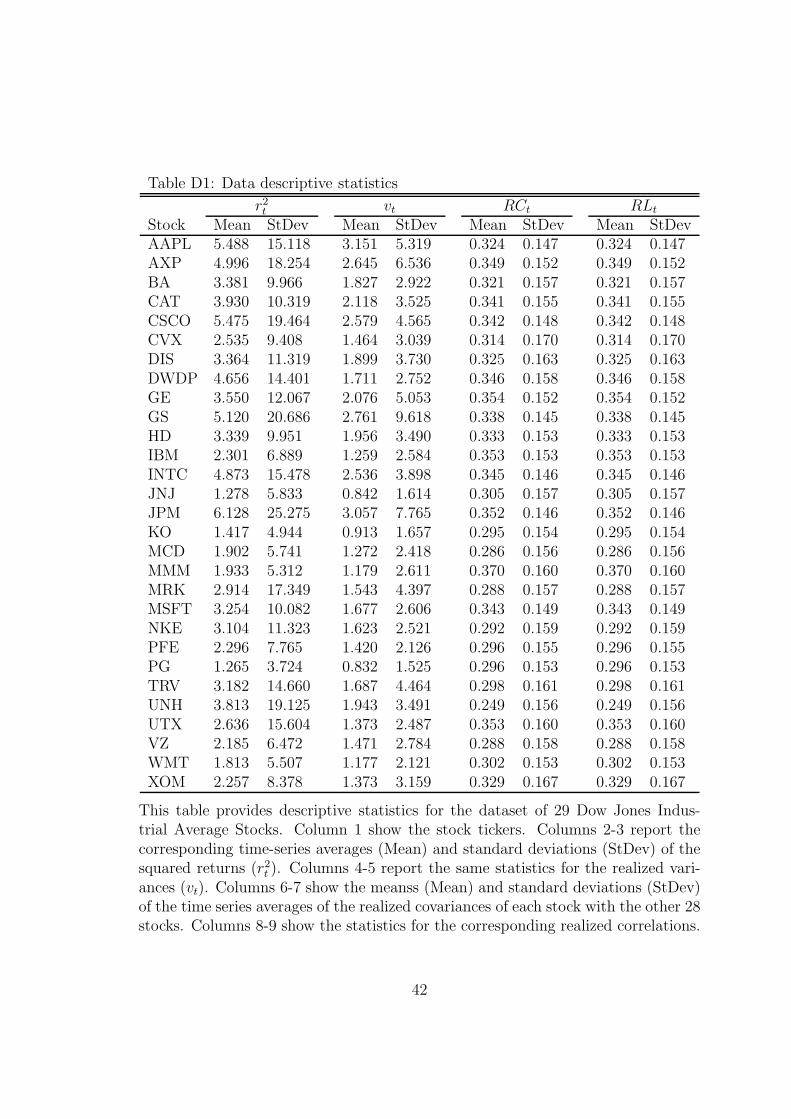
Descriptive statistics are provided in Table D1 of the SA. For each stock, itreports the time-series averages and standard deviations of its squared returns andrealized variances, and the means and standard deviations of the time series averagesof its realized covariances and correlations with the other 28 stocks. Each averagerealized variance does not account for the overnight variation and is therefore afraction (in most cases 50 to 60 percent) of the corresponding average squared return.
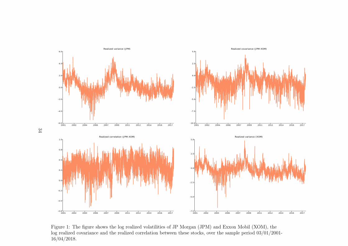
Figure 1 shows a representative example of time series plots of the realized vari-ances of two stocks (JPM and XOM) and the corresponding realized covariancesand correlations.
Insert Figure 1 here
The focus of the empirical application is a forecasting comparison of the con-ditional covariance and correlation matrices, and the conditional variances of the29 stocks using a set of models. Before reporting the results of the comparisons,estimation results are reported for the DCC and DECO models.
17
5.2 Estimation Results for the Full Period
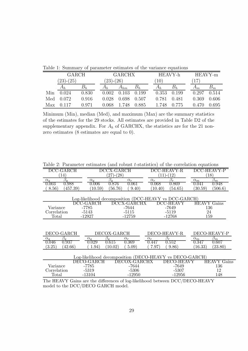
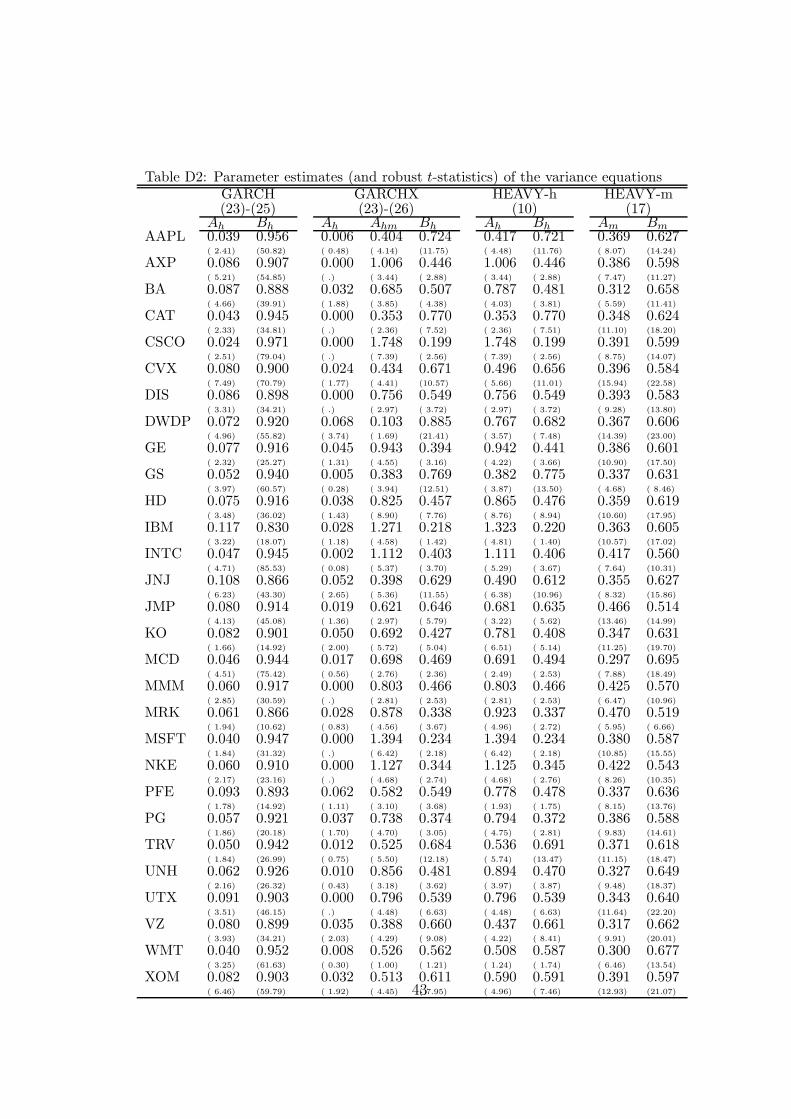
Table 1 presents summary statistics (median, minimum, maximum) of the first stepparameter estimates (except the constant terms) of the 29 variance equations ofthe GARCH, GARCHX, HEAVY-h and HEAVY-m models. The estimates for eachstock, and the associated robust t-statistics, are given in Table D2 of the SA.
Insert Table 1 here
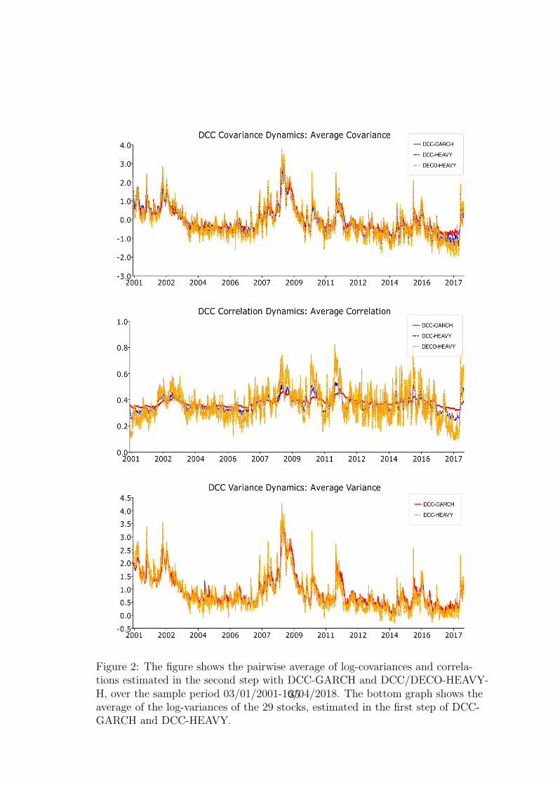
The estimates of the Bh parameters in the HEAVY-h model are smaller thanin the GARCH model (median of 0.481 versus 0.916), while the estimates of theAh parameters are much larger (medians of 0.781 versus 0.072). The influenceof these differences is visible on the bottom panel of Figure 2, which shows (inlog) the time-series of the average (over the 29 stocks) of the corresponding fittedconditional variances. The GARCH path is smoother than the HEAVY-h path,and the latter fluctuates locally more strongly than the former, responding faster torecent changes of volatility. Similar differences occur for each stock. The GARCHparameter estimates are much more homogenous across the different stocks than theHEAVY-h estimates. The values of the HEAVY-m parameter estimates are moresimilar to HEAVY-h than to GARCH, though they are much more homogenousthan for HEAVY-h.
In the nesting GARCHX model, the coefficient (in Ah) of the lagged squaredreturn is set to zero for eight stocks out of 29 because a non-negativity constraintis imposed and is binding; for these stocks, GARCHX estimates are identical toHEAVY-h. For the 21 other stocks, the estimate is positive (between 0.002 and0.068), with t-statistics below 1.5 in 12 cases (out of 21), and 4 larger than two. Eventhough the t-statistic has a non-standard distribution since the null hypothesis ofzero is on the boundary of the parameter space, these results suggest that for almostall stocks, the estimate is not significant. On the contrary, the estimate of the laggedrealized variance coefficient (in Amh) is positive (between 0.103 and 1.748, with 0.698as median value) and the associated t-statistics are usually large enough to suggestthey are significant (only three are below 2.5). The log-likelihood gain of GARCHXover HEAVY-h is equal to 5 for the 21 additional parameters, hence it appears tobe minor. On the contrary, the gains of GARCHX and HEAVY-h over GARCH aresubstantial (41 and 36 respectively). Notice that GARCH and HEAVY-h are notnested, but they have the same number of parameters, so choosing between themusing their log-likelihood values is equivalent to a choice based on model choicecriteria. In brief, these results suggest that the conditional variance dynamics isbetter captured by the lagged realized variance than by the lagged squared return,confirming the findings of Shephard and Sheppard (2010).
Insert Figure 2 here
18
Table 2 presents the second step parameter estimates of the correlation models:DCC-GARCH, DCCX-GARCH, DCC-HEAVY-R (eq. (11)-(12)), DCC-HEAVY-P (eq. (18)), and the corresponding DECO versions. For the DCC models, theseestimates are broadly in line with those of the variance equations. The estimate of βr
in DCC-HEAVY-R model is smaller than that of βq in DCC-GARCH model (0.869versus 0.988), and the estimate of αr is larger than that of αq (0.068 versus 0.003),implying less smooth and more reactive fitted correlations. The paths of averagefitted correlations and covariances of the three models are shown on Figure 2. Thepaths of the DECO-HEAVY-R model are much less smooth and more reactive torecent information than for DCC-HEAVY-R, due to a smaller estimate of βr (0.552versus 0.869) and a larger one of αr (0.447 versus 0.068). The paths for the DCC-GARCH are smoother and less reactive than in the HEAVY models. The describedpath differences are stronger for each pair of stocks, since averaging reduces thevariability.
Insert Table 2 here
In the nesting DCCX- and DECOX-GARCH models, the coefficient estimatesof the lagged realized correlation (0.068 and 0.447) are of the same magnitude asin the DCC- and DECO-HEAVY-R (0.061 and 0.369), with large t-statistics (9.40for DCCX, 5.09 for DECOX). The coefficient estimate of the lagged return cross-product is very close to zero (with t-statistic 10.59) in DCCX, while it is equal to0.029 (with t-statistic 1.94) in DECOX. The maximized second step log-likelihoodvalues of DCCX-GARCH (−5115) and DCC-HEAVY (−5119) are slightly different,but they are much larger than the value of DCC-GARCH (−5143). For the DECOmodels: DECO-HEAVY (−5307) and DECOX-GARCH (−5306) are very close,but DECO-GARCH (−5319) is lower. Thus lagged realized correlations can beconsidered as more important drivers of the conditional correlations rather thanreturn cross-products.
The maximized log-likelihood values and their decomposition into the varianceand correlation parts are reported in Table 2. The decompositions suggest that theDCC-HEAVY and the DECO-HEAVY dominate the DCC-GARCH model in boththe variance and correlation parts. However, most of the in-sample gain is comingfrom the variance part. The overall improvement is substantial. DCC-HEAVYimproves slightly more than DECO-HEAVY. Notice that these models have the samenumber of parameters, so comparisons using log-likelihood values are equivalent tocomparisons using model choice criteria
19
5.3 Forecasting Comparisons
A comparison of models can be made by evaluating the in-sample and out-of-sampleforecasting performances of the models using the Model Confidence Set (MCS) ofHansen et al. (2011). A MCS identifies a set of models having the best forecast-ing performance at a chosen confidence level, based on a loss function. Six mod-els are compared: DCC-GARCH, DCC-HEAVY, DECO-GARCH, DECO-HEAVY,BEKK-GARCH, BEKK-HEAVY. Out-of-sample s-step-ahead forecasts of the 29-dimensional covariance and correlation matrices are computed, for s=1, 5 and 22;for horizons 5 and 22, they are iterated forecasts. For DECO models, the correlationsare computed from DECO itself, not from the underlying DCC.
5.3.1 Loss Functions
Statistical and economic loss functions are adopted along the lines proposed byBecker et al. (2015).
For the covariance matrix forecasts, two statistical loss functions are used, whichcompare the covariance matrix forecasts with respect to the actual (unobserved)covariance matrix Σt+s. The first one is based on the negative of the Wishart log-density function:
QLIKat,s(Σt+s, H
at+s|t) = tr[(Ha
t+s|t)−1Σt+s] + log |Ha
t+s|t|, (44)
where Hat+s|t denotes the s-step forecast using model a conditional on time t infor-
mation. The second loss function is based on the Frobenius norm of the differencebetween the forecast and benchmark matrices (see e.g. Golosnoy et al., 2012), de-fined by
FNat,s = ||Σt+s −Ha
t+s|t|| =
[
∑
i,j
(σij,t+s − haij,t+s)
2
]1/2
. (45)
Since Σt+s is unobservable, the observed realized covariance matrix RCt+s is used asproxy for it. These statistical loss functions provide a consistent ranking of volatilitymodels in the sense of Patton (2011) and Patton and Sheppard (2009) as they arerobust to noise in the proxy; see also Laurent et al. (2013).
For the correlation matrix forecasts, the QLIK and FN losses are computed fromthe same formulas as for covariances, that is (44) and (45). The only difference isthat forecasted correlations and realized correlations replace forecasted covariancesand realized covariances, respectively.
Once a time series of Th,s (covariance or correlation) forecasts is obtained for a
20
model, the corresponding losses and their time series average are computed, i.e.
QLIKas =
1
Th,s
Th,s∑
t=1
QLIKat,s, and FNa
s =1
Th,s
Th,s∑
t=1
FNai,t,s. (46)
This is performed for each model and each forecast horizon, so that models canbe ranked by the MSC procedure and a MCS at a chosen confidence level can beidentified.
For the variance forecasts of different models, we use the univariate loss functions
UQLIKai,t,s =
vi,t+s
hai,t+s|t
− log
(
vi,t+s
hai,t+s|t
)
− 1, (47)
andMSEa
i,t,s = (vi,t+s − hai,t+s|t)
2, (48)
where vi,t+s is the observed realized variance of stock i at date t + s and hai,t+s|t is
the corresponding s-step forecast of model a, based on information available at datet. Once the time series average of each loss function has been computed for eachstock, the mean across stocks is taken and used in the MCS procedure, i.e.
UQLIKas =
1
Th,sk
Th,s∑
t=1
k∑
i=1
QLIKai,t,s, and MSEa
s =1
Th,sk
Th,s∑
t=1
k∑
i=1
MSEai,t,s. (49)
The economic loss functions are relevant for the covariance matrix forecasts.They are based on forecasted portfolio performances. The same economic loss func-tions as Engle and Kelly (2012) are used: global minimum variance portfolio (GMV),and minimum variance portfolio (MV); see also Engle and Colacito (2006). Theseloss functions are based on the variances of the forecasts of portfolio returns. Asuperior model produces optimal portfolios with lower forecast variance. Given acovariance matrix forecast Ha
t+s|t, the GMV portfolio weight vector wat+s is computed
as the minimizer of the portfolio variance (wat+s)
′Hat+s|tw
at+s subject to the constraint
that the weights add to unity. Once this is done for each forecast date, the GMVloss function is the average of the portfolio variances over the forecast period:
GMV as =
1
Th,s
Th,s∑
t=1
(wat+s)
′Hat+s|tw
at+s. (50)
The MV portfolio is obtained by minimizing the portfolio variance subject tothe additional constraint that the expected portfolio return be larger than a chosenvalue. Following Engle and Kelly (2012), this value is fixed at q = 10% and the
21
expected portfolio return (µ) at the mean of the data. The MV loss is defined like(50) but with the optimal weight vectors corresponding to the MV minimizations.The optimal GMV and MV weights are analytically known functions of Ha
t+s|t, and
of µ and q for MV (see e.g. Engle and Kelly, 2012).
5.3.2 Results
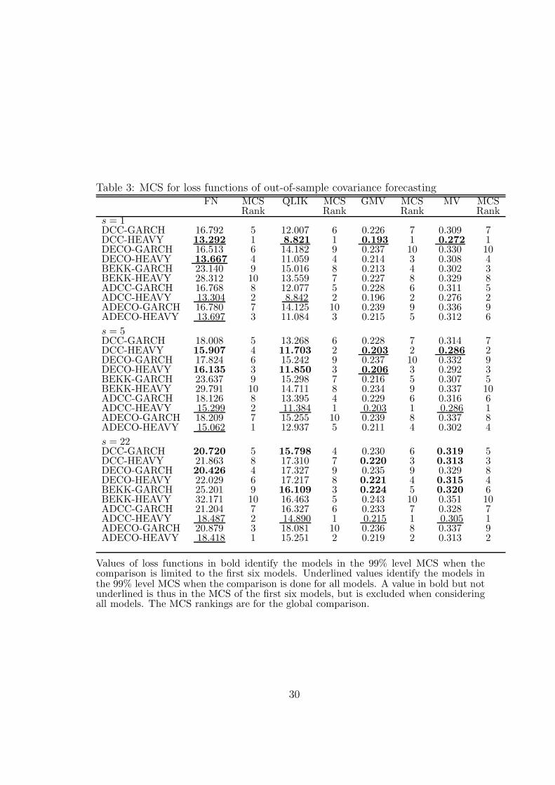
To compute out-of-sample forecasts, each model is re-estimated every 5th observa-tion based on rolling sample windows of 3,000 observations, resulting in a total ofTh = 1318 out-of-sample forecasts for s = 1, 1314 for s = 5, and 1297 for s = 22.
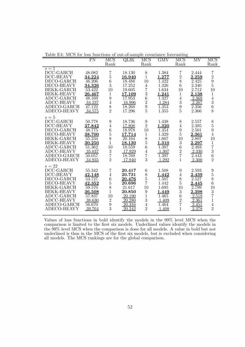
Table 3 reports the out-of-sample forecast losses defined by (46) and the economicloss functions, for the different models. The boldface values identify the models thatbelong to the 99% model confidence set (MCS99 hereafter) for each loss function,when the comparison is limited to the six symmetric models mentioned in the firstparagraph of this subsection. The comparisons including the four asymmetric mod-els included in the table are presented in subsection 5.4, and the MCS ranks in thetable pertain to the comparisons of all models.
At forecast horizons 1 and 5, DCC-HEAVY belongs to the MCS99 for all lossfunctions, DECO-HEAVY belongs to it for a subset of loss functions, and all theother models are out of each MCS99. At horizon 22, no HEAVY model is in MCS99of FN and QLIK; MCS99 includes DCC-GARCH and DECO-GARCH for FN andDCC-GARCH and BEKK-GARCH for QLIK For the GMV loss function, MCS99consists of DCC-HEAVY, DECO-HEAVY and BEKK-GARCH, and for MV loss, itcontains DCC-GARCH, DECO-HEAVY and BEKK-GARCH.
Insert Table 3 and 4 here
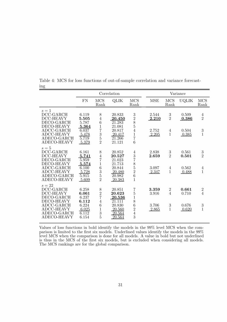
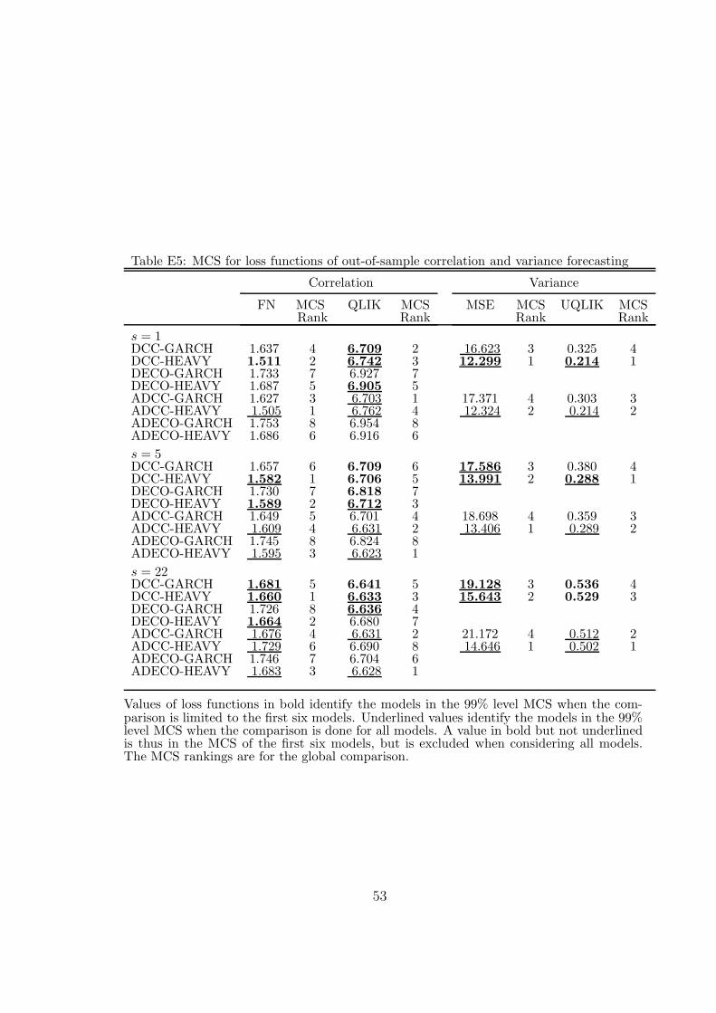
Table 4 reports the MCS99 sets for correlation and variance forecasts separately,excluding the BEKK models for these comparisons, and using only the statisticalloss functions since the economic loss functions use the covariance matrix.
For correlations, DCC-HEAVY is in MCS99 of both loss functions at the threehorizons. DECO-HEAVY is also in the MCS99 of FN at the three horizons, andDECO-GARCH in the QLIK MCS99 set at horizon 22.
For variances, the loss values defined by (47) are reported in the ‘Variance’ partof Table 4. Notice that DECO models are irrelevant (being the same as DCC in thefirst step of estimation). The results reveal that DCC-HEAVY is alone in MCS99for both MSE and QLIK at horizons 1 and 5. At horizon 22, only DCC-GARCH isin both MCS99 sets. Shephard and Sheppard (2010) report that the performanceof HEAVY with respect to GARCH deteriorates as the forecast horizon increases.
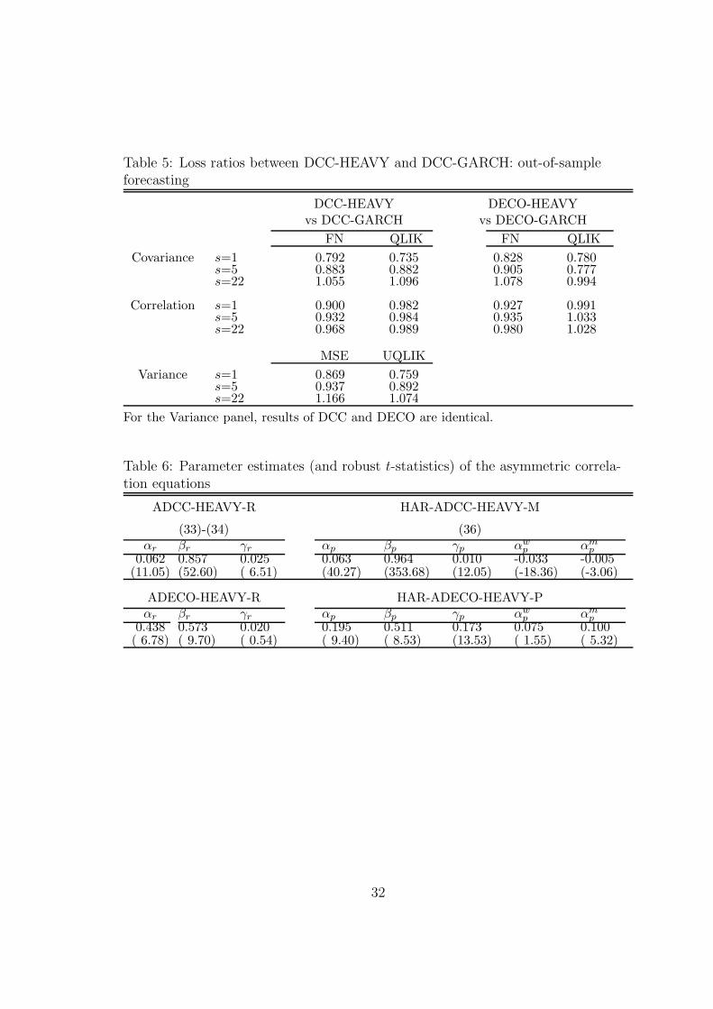
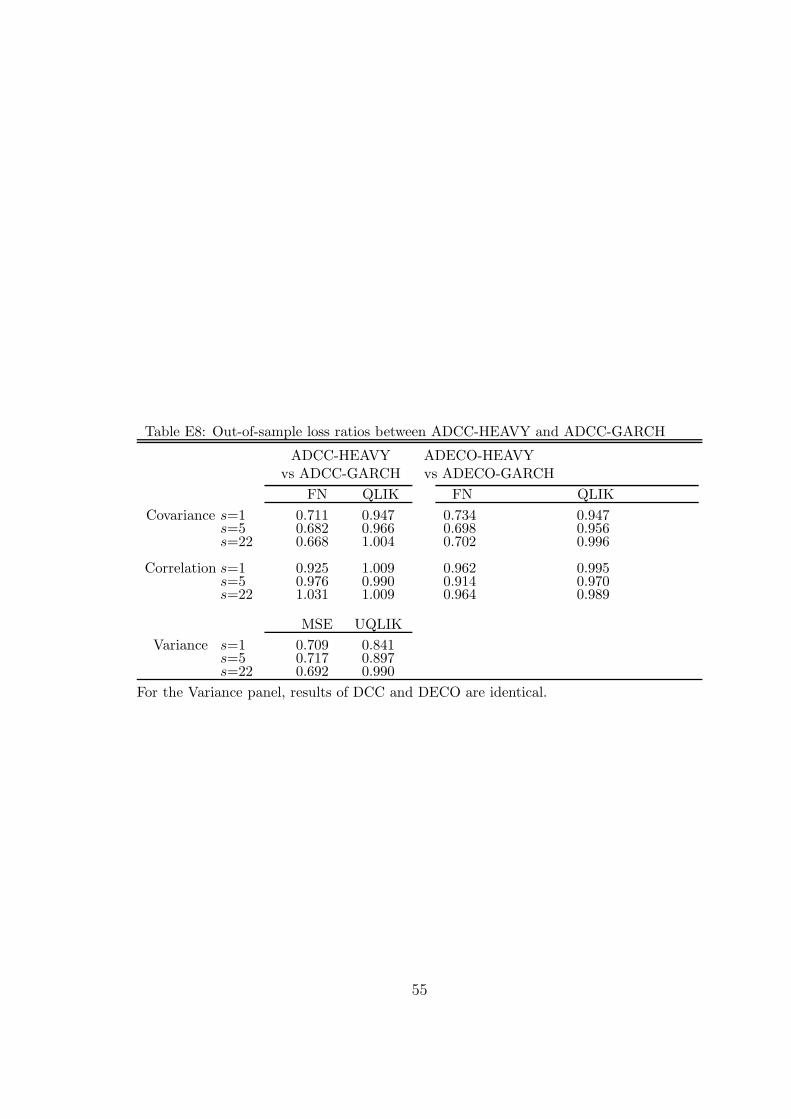
To trace where the forecast gains occur, Table 5 reports the ratios betweenthe losses of the DCC-HEAVY and DCC-GARCH models, and likewise for the
22
DECO models. One can see that the DCC/DECO-HEAVY models outperform theDCC/DECO-GARCH models both in covariance, correlation and variance forecastlosses at the forecast horizons 1 and 5 (with a single exception for DECO). Theimprovements are larger for horizon 1 than 5, and smaller for DECO than for DCC(except one case). They can be important, e.g. DCC-HEAVY reduces the covarianceand variance QLIK losses by 10% at least and up to 25%. At horizon 22, the GARCHmodels have the smallest losses, except for correlations where the differences are lessthan 2.5%. The loss improvements of GARCH with respect to HEAVY are between7 and 17% when they occur.
Insert Table 5 here
In brief, the forecast comparisons are clearly favouring the DCC-HEAVY modelat the short forecast horizons for all loss functions, and to a lesser extent the DECO-HEAVY model, at the expense of the BEKK-HEAVY and the three GARCH models.At the longest forecast horizon, the results depend on the loss function; moreoverthere is a clear worse performance of DCC-HEAVY relative to DCC-GARCH forvariance and covariance forecasts at this horizon.
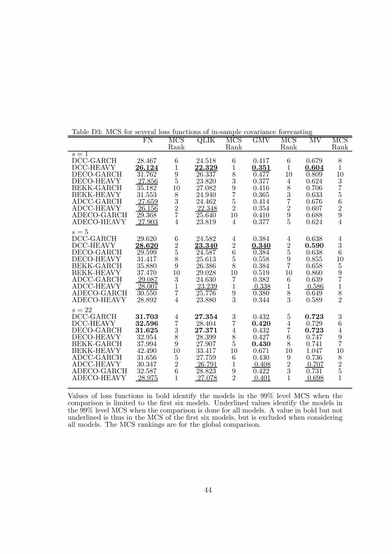
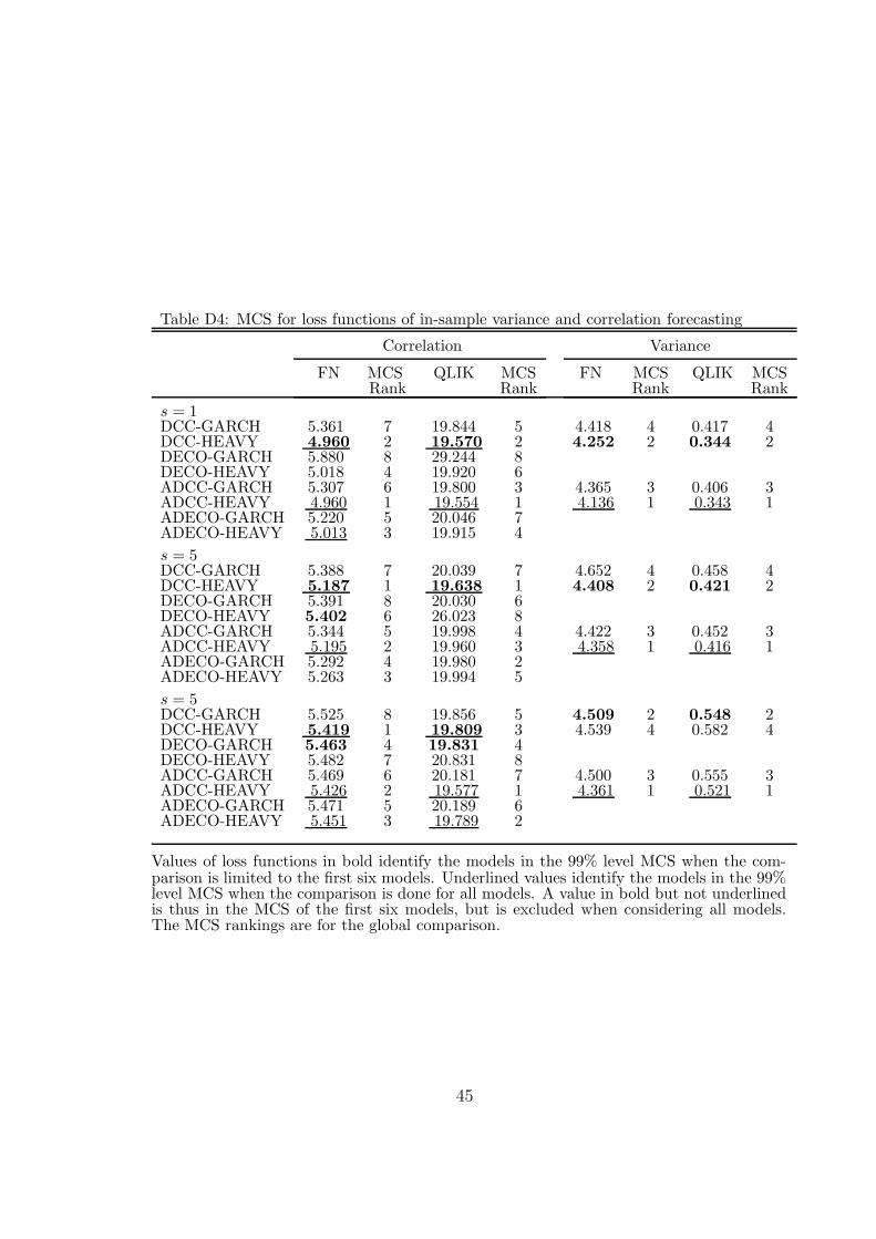
The in-sample forecasting results are reported in the SA (Tables D3-D4). Theydo not differ much from the out-of-sample results.
5.4 Asymmetric and HAR Terms in DCC/DECO-HEAVY
The out-of-sample forecast performance of the DCC-HEAVY model deteriorateswith respect to DCC-GARCH when the forecast horizon increases, switching frombetter to worse at some horizon between 5 and 22. DCC-HEAVY makes use of fore-casts of realized variances and correlations. If the realized variance or correlationequations are incorrectly specified, the forecast error is brought to the conditionalcovariance and correlation forecasts. These forecast errors get larger when the fore-cast horizon is longer. To improve the forecast performance of DCC-HEAVY inmultiple step ahead forecasts, the ADCC-HEAVY model defined by (32)-(34)-(35)-(36) is worth trying. The HAR terms are useful to capture the long memory featureof realized variances and correlations.
5.4.1 Estimation Results
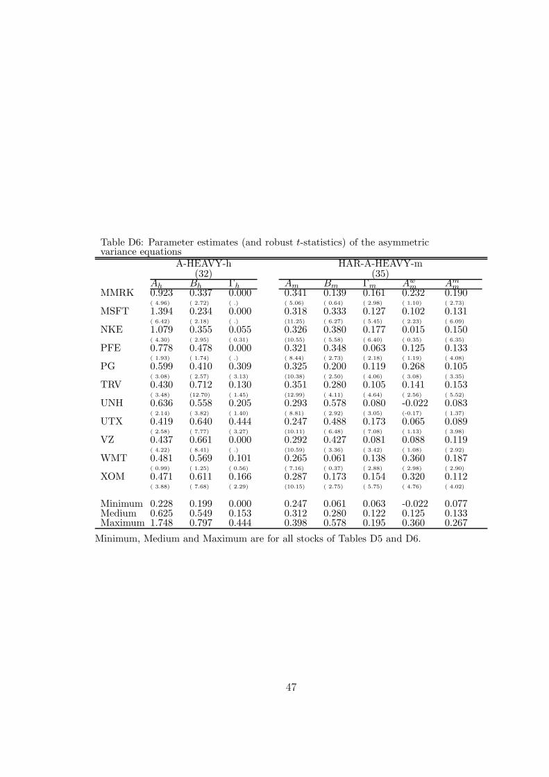
The parameter estimates of the asymmetric variance equations are reported in theSA (Tables D5 and D6). For the conditional variances, the coefficient estimates ofthe asymmetric term (the diagonal elements of Γh in (32)) are positive for 22 stocks,with t-statistics above 2 for eight of them. For the realized variances, the coefficient
23
estimates of the asymmetric term (the diagonal elements of Γm in (35)) are allpositive, with t-statistics larger than 2.5 for 28 stocks. The coefficient estimatesof the weekly HAR term are positive (with a single, insignificant, exception) butonly fourteen of them have t-statistics above 2, indicating a moderate impact of thisterm. On the contrary, the monthly HAR term is positive for all stocks and appearsto be strongly significant (with one exception).
The estimates of the asymmetric correlation equations are reported in Table 6.For the conditional correlations, the estimate of γr is positive in the ADCC (0.025)and very significant (t-statistic 6.51). This means that the impact of each laggedrealized correlation on the next conditional correlation is stronger (being equal to0.062+0.025) when both lagged returns of the corresponding assets are negativethan otherwise (being then equal to 0.062). Nevertheless, the additional statisticallysignificant impact of 0.025 is not very important on the next period correlation, sinceit increases it by 2.5% of the previous period correlation (if both lagged returns arenegative): that means an increase of 0.0125 if the previous correlation is 0.5. Forthe ADECO model, the impact is of 2% and statistically insignificant.
Insert Table 6 here
For the realized correlations, the estimate of γp is positive and significant inboth models (HAR-ADCC and HAR-ADECO), which means that the impact ofeach lagged realized correlation on the next conditional mean of the realized corre-lation is stronger (being equal to 0.063+0.010 in the HAR-ADCC) when both laggedreturns of the corresponding assets are negative than otherwise (being then equal to0.063). The same remark applies as above, about the limited value of the expectedcorrelation change this implies between two consecutive days.
Concerning the HAR terms, the weekly term impact is negative (-0.033) andsignificant in HAR-ADCC, positive (0.075) and insignificant in HAR-ADECO. Themonthly term impact is negative in HAR-ADCC but positive in HAR-ADECO,being significant in both models. Anyway, the effective daily changes of expectedcorrelations these terms imply are small in HAR-ADCC and moderate in HAR-ADECO.
5.4.2 Forecast Comparisons
For covariance forecasts, Table 3 reports the loss function values for the four asym-metric models (ADCC-HEAVY, ADECO-HEAVY, ADCC-GARCH and ADECO-GARCH) in addition to the six symmetric models. The MCS99 for each loss functionand horizon is identified by the underlined values; a bold underlined value is thusin the MCS99 for the ten models, and in that of the first six models, while a bold
24
value, not underlined, is in the MCS99 of the first six models but is removed fromthe MCS99 when the ten models are compared.
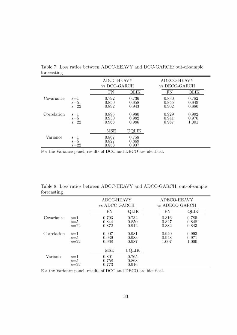
The changes of the MCS99 due to the inclusion of the four asymmetric models inthe comparisons are in favour of HEAVY models: the asymmetric HEAVY modelsare added to the MCS99 of some loss functions and horizons, but no asymmetricGARCH is model added for any loss function and horizon. For example, at horizons 5and 22, ADCC-HEAVY is in the MCS99 sets for all loss functions; only the ADECO-HEAVY model also belongs to these sets in the case of the FN loss. The asymmetricHEAVY models attenuate or even reverse the worse performance of their symmetriccounterparts relative to DCC at the three horizons, as can be seen by comparingthe covariance loss ratios reported in Tables 7 and 8 and the corresponding valuesin Table 5.
For correlation forecasting, Table 4 also includes the asymmetric models in thecomparisons. The changes of the MCS99 due to this are mixed: at horizon 1, only theasymmetric versions of the HEAVY models that were in the initial MCS99 are added;at horizon 5, ADCC- and ADECO-HEAVY are added for both losses; at horizon22, ADECO-HEAVY is added for FN loss, being alone in MCS99; for QLIK loss,ADCC-HEAVY, ADECO-GARCH and ADECO-HEAVY are added, DCC-HEAVYbeing removed and DECO-GARCH kept. The correlation loss ratios reported inTables 7 and 8 differ slightly from those of Table 5, indicating that the asymmetricversions of the models do not improve much the symmetric versions.
For variance forecasting (Table 4), the main change in the MCS99 due to theinclusion of asymmetric models is that ADCC-HEAVY is added for both loss func-tions and all horizons, being even the single model in the sets at horizons 5 and 22.This model has the rank 1 in all comparisons. Clearly, ADCC-HEAVY improvesvariance forecasting, especially at horizons larger than 1. Loss ratios show that thisimprovement is important at horizon 22; for example, for MSE loss, it goes from-16.6% in Table 5 to +14.7% in Table 7 and +22.7% in Table 8.
Insert Tables 7 and 8 here
6 Conclusions
Multivariate volatility models that specify the dynamics of the daily conditionalcovariance matrix as a function of realized covariances have emerged in the literaturesince 2012. They are a valuable alternative to multivariate GARCH models whereinthe dynamics depend on lagged squared returns and their cross-products, becauserealized variances and covariances are more precise measures of daily volatility.
Perhaps surprisingly, with the partial exception of Braione (2016), no dynamicconditional correlation formulation of a HEAVY model has been proposed in the
25
literature, where BEKK-type formulations are used in the papers of Noureldin etal. (2012) and Opschoor et al. (2018). Our contribution fills this gap by devel-oping DCC-type HEAVY models. Such models have the advantage, with respectto BEKK models, of separating the specification of the conditional variances fromthe specification of the conditional correlations. The same advantage occurs in thespecifications of the expected realized variances and correlations. As for GARCHDCC models, this results in more flexible models, in the sense that the dynamics ofvariances is different between assets and from the dynamics of correlations. Stickingto scalar models for correlations, the models remain parsimonious in parameters.
An illustrative empirical application for twenty-nine assets illustrates the valueof the flexibility of DCC and DECO versions of HEAVY models. These models,including extensions to include asymmetric effects, have superior forecasting per-formance with respect to BEKK formulations. As always in this type of empiricalexercise, this finding is contingent to the dataset used and cannot be claimed tobe valid in general. A robust conclusion is that HEAVY models dominate GARCHversions in term of forecasting performance.
This research has not developed the properties of the QML estimators of theparameters of the DCC- and DECO-HEAVY models. Such developments and addi-tional empirical studies will come out of future research.
Acknowledgments
Thanks to Professors Lyudmila Grigoryeva (University of Konstanz) and Juan-PabloOrtega (University of St.Gallen) for providing the datasets for the DJIA companiesand to Oleksandra Kukharenko (University of Konstanz) for handling the data andcomputing the realized covariance matrices from the TAQ data.
References
[1] Aielli, G. (2013). Dynamic conditional correlation: on properties and estima-tion. Journal of Business & Economic Statistics 31, 282-299.
[2] Bauwens, L., Laurent, S. and Rombouts, J. V. K. (2006). Multivariate GARCHmodels: a survey. Journal of Applied Econometrics, 21, 79-109.
[3] Bauwens, L., Storti, G. and Violante, F. (2012). Dynamic conditional correla-tion models for realized covariance matrices. CORE DP 2012/60.
26
[4] Bauwens, L., Braione, M. and Storti, G. (2016). Forecasting Comparison ofLong Term Component Dynamic Models for Realized Covariance Matrices. An-nals of Economics and Statistics, 123/124, 103-134.
[5] Braione, M. (2016). A time-varying long run HEAVY model. Statistics andProbability Letters, 119, 36-44.
[6] Chiriac, R. and Voev, V. (2011). Modelling and forecasting multivariate realizedvolatility. Journal of Applied Econometrics, 26, 922-947.
[7] Corsi, F. (2009). A simple approximate long-memory model of realized volatil-ity. Journal of Financial Econometrics, 7, 174-196.
[8] Engle, R.F. (2002). Dynamic conditional correlation: A simple class of multi-variate generalized autoregressive conditional heteroskedasticity models. Jour-nal of Business & Economic Statistics, 20, 339-350.
[9] Engle, R.F. and Kroner, K. (1995). Multivariate simultaneous generalizedARCH. Econometric Theory, 11, 122-150.
[10] Engle, R. F. and Gallo, G. M. (2006). A multiple indicator model for volatilityusing intra-daily data. Journal of Econometrics, 131, 3-27.
[11] Engle, R.F. and Kelly, B. (2012). Dynamic equicorrelation. Journal of Business& Economic Statistics, 30, 212-228.
[12] Engle, R. F. and Sheppard, K. (2001). Theoretical and empirical propertiesof dynamic conditional correlation multivariate GARCH. WP 8554, NationalBureau of Economic Research.
[13] Engle, R. F., Hendry, D. F. and Richard, J.-F. (1983). Exogeneity. Economet-rica, 51, 277-304.
[14] Gourieroux, C., Jasiak, J. and Sufana, R. (2009). The Wishart autoregressiveprocess of multivariate stochastic volatility. Journal of Econometrics, 150, 167-181.
[15] Golosnoy, V., Gribisch, B. and Liesenfeld, R. (2012). The conditional autore-gressive Wishart model for multivariate stock market volatility. Journal ofEconometrics, 167, 211-223.
[16] Gorgi, P., Hansen, P.R., Janus, P. and Koopman, S.J. (2019). Realized Wishart-GARCH: A Score-driven Multi-Asset Volatility Model. Journal of FinancialEconometrics, 17, 1-32.
27
[17] Hansen, P. R., Lunde, A. and Nason, J.M. (2011). The model confidence set.Econometrica, 79, 453-497.
[18] Hansen, P. R., Huang, Z. and Shek H. (2012). Realized GARCH: A Joint Modelof Returns and Realized Measures of Volatility. Journal of Applied Econometrics27, 877-906.
[19] Hansen, P. R., Lunde, A. and Voev, V. (2014). Realized Beta GARCH: AMultivariate GARCH Model with Realized Measures of Volatility. Journal ofApplied Econometrics 29, 774-799.
[20] Jin, X. and Maheu, J. M. (2012). Modeling realized covariances and returns.Journal of Financial Econometrics, 11, 335-369.
[21] Laurent, S., Rombouts, J. V. and Violante, F. (2013). On loss functions andranking forecasting performances of multivariate volatility models. Journal ofEconometrics, 173, 1-10.
[22] Noureldin, D., Shephard, N. and Sheppard, K. (2012). Multivariate high-frequency-based volatility (HEAVY) models. Journal of Applied Econometrics,27, 907-933.
[23] Oh, D. H. and Patton, A. J. (2016). High-dimensional copula-based distribu-tions with mixed frequency data. Journal of Econometrics, 193, 349-366.
[24] Opschoor, A., Janus, P., Lucas, A. and Van Dijk, D. (2018). New HEAVYmodels for fat-tailed realized covariances and returns. Journal of Business &Economic Statistics, 1-15.
[25] Patton A.J. (2011). Volatility forecast comparison using imperfect volatilityproxies. Journal of Econometrics 160, 246-256.
[26] Patton A.J and Sheppard K.K. (2009). Evaluating volatility and correlationforecasts. In Handbook of Financial Time Series, Andersen TG, Davis RA,Kreiss JP, Mikosch T (eds). Springer: Berlin; 801-838.
[27] Shephard, N. and Sheppard, K. (2010). Realising the future: forecasting withhigh-frequency-based volatility (HEAVY) models. Journal of Applied Econo-metrics, 25, 197-231.
[28] Sheppard, K. and Xu, W. (2019). Factor High-Frequency-Based Volatility(HEAVY) Models. Journal of Financial Econometrics, 17, 33-65.
28
Table 1: Summary of parameter estimates of the variance equations
Minimum (Min), median (Med), and maximum (Max) are the summary statisticsof the estimates for the 29 stocks. All estimates are provided in Table D2 of thesupplementary appendix. For Ah of GARCHX, the statistics are for the 21 non-zero estimates (8 estimates are equal to 0).
Table 2: Parameter estimates (and robust t-statistics) of the correlation equationsDCC-GARCH DCCX-GARCH DCC-HEAVY-R DCC-HEAVY-P
Values of loss functions in bold identify the models in the 99% level MCS when thecomparison is limited to the first six models. Underlined values identify the models inthe 99% level MCS when the comparison is done for all models. A value in bold but notunderlined is thus in the MCS of the first six models, but is excluded when consideringall models. The MCS rankings are for the global comparison.
30
Table 4: MCS for loss functions of out-of-sample correlation and variance forecast-ing
Values of loss functions in bold identify the models in the 99% level MCS when the com-parison is limited to the first six models. Underlined values identify the models in the 99%level MCS when the comparison is done for all models. A value in bold but not underlinedis thus in the MCS of the first six models, but is excluded when considering all models.The MCS rankings are for the global comparison.
31
Table 5: Loss ratios between DCC-HEAVY and DCC-GARCH: out-of-sampleforecasting
Figure 1: The figure shows the log realized volatilities of JP Morgan (JPM) and Exxon Mobil (XOM), thelog realized covariance and the realized correlation between these stocks, over the sample period 03/01/2001-16/04/2018.
34
Figure 2: The figure shows the pairwise average of log-covariances and correla-tions estimated in the second step with DCC-GARCH and DCC/DECO-HEAVY-H, over the sample period 03/01/2001-16/04/2018. The bottom graph shows theaverage of the log-variances of the 29 stocks, estimated in the first step of DCC-GARCH and DCC-HEAVY.
35
Supplementary Appendix
A The scalar BEKK-HEAVY model
A1 Equivalence with a covariance targeting version of NSS
The specification (5) of Ht can be obtained from the non-targeting version:
Ht = CH + αHRCt−1 + βHHt−1;
where CH is a constant PD matrix. By taking the unconditional expectation, weobtain E(Ht) = CH +αHE(RCt−1)+βHE(Ht−1) so that CH = (1−β)H−αM . Weshow that the equation (5) is equivalent to the equation obtained from the BEKK-HEAVY equation (11) of NSS (Noureldin et al. 2012), assuming the scalar version.Equation (11) of NSS, in the non-scalar version, is
where AH and BH are k∗ × k∗, with k∗ = k(k + 1)/2), matrices of parameters (seeequation (7) of NSS), Lk is the k∗ × k2 elimination matrix such that vech(Ht) =Lkvec(Ht), Dk is the k2 × k∗ duplication matrix such that vec(Ht) = Lkvech(Ht),LkDk = Ik∗ , and
K = Lk(K ⊗ K)Dk = Lk(M ⊗ H−1)Dk
with K = M1/2H−1/2, so that
K ⊗ K = (M1/2H−1/2)⊗ (M1/2H−1/2) = M ⊗ H−1.
In the scalar specification,
BH = Lk(√
βHIk ⊗√
βHIk)Dk = βHLkIk2Dk = βHIk∗.
and likewiseAH = αHIk∗ .
We transform the vech(Ht) equation above to an equation for vec(Ht) by pre-multiplying both sides by Dk and using the scalar versions of BH and AH :
The matrix (1− βH)H − αHM may not be PD for all values of (αH , βH) restrictedby αH ≥ 0, 0 ≤ βH < 1. 1
Assumption 2 in NSS is that the spectral radius of BH +AHK, a k∗×k∗ matrix,is less than unity. In the scalar case, BH + AHK = βHIk∗ + αHLk(M ⊗ H−1)Dk.This is the matrix subtracted form Ik∗ in the constant term: so, if its spectral radiusis less than unity, the smallest eigenvalue of Ik∗ − βHIk∗ − αHK is positive, hencethe intercept matrix of Ht is PD (being the product of two PD matrices). Thus theassumption 2 of NSS implies that (1−βH)H−αHM is PD. In practice, this matrixis not PD for all (αH , βH) restricted only by αH ≥ 0, βH ≥ 0, and βH < 1, so inestimation this has to be ensured.
For estimation, in practice we check that Ht, rather than (1− βH)H −αHM ,2 ispositive definite for each t in the sample period during the numerical maximizing ofthe log-likelihood function. For both datasets we use, no lack of PDness occurred.Figure 3 shows the parameter values for which Ht becomes non-PD for some t inthe sample period for the data used in the empirical application reported in Section5. The figure shows that the PDness regions is a large subset of the usual triangle
1For example, for k = 2, if βH = 0 and h21 = 0, the determinant of (1− βH)H −αHM is equalto h11h22 + α2|M | − α(h11m22 + h22m11), which may be negative because of the last term.
2In the same setup as in the previous footnote, hii,t = hii + αH(RCii,t−1 − mii) (i = 1 or 2),and h21,t = αH(RC21,t−1 − m21). If RC11,t−1 − m11 = RC22,t−1 − m22 = 0, the determinant ofHt, equal to h11h22 − α2
H(RC21,t−1 − m21)2, may be negative.
37
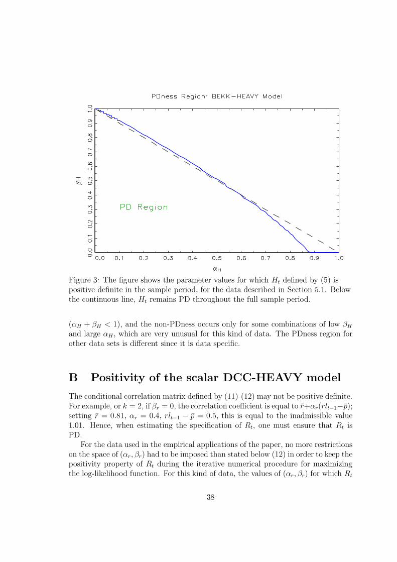
Figure 3: The figure shows the parameter values for which Ht defined by (5) ispositive definite in the sample period, for the data described in Section 5.1. Belowthe continuous line, Ht remains PD throughout the full sample period.
(αH + βH < 1), and the non-PDness occurs only for some combinations of low βH
and large αH , which are very unusual for this kind of data. The PDness region forother data sets is different since it is data specific.
B Positivity of the scalar DCC-HEAVY model
The conditional correlation matrix defined by (11)-(12) may not be positive definite.For example, or k = 2, if βr = 0, the correlation coefficient is equal to r+αr(rlt−1−p);setting r = 0.81, αr = 0.4, rlt−1 − p = 0.5, this is equal to the inadmissible value1.01. Hence, when estimating the specification of Rt, one must ensure that Rt isPD.
For the data used in the empirical applications of the paper, no more restrictionson the space of (αr, βr) had to be imposed than stated below (12) in order to keep thepositivity property of Rt during the iterative numerical procedure for maximizingthe log-likelihood function. For this kind of data, the values of (αr, βr) for which Rt
38
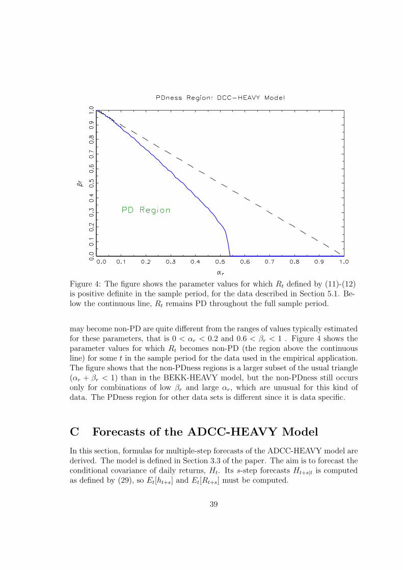
Figure 4: The figure shows the parameter values for which Rt defined by (11)-(12)is positive definite in the sample period, for the data described in Section 5.1. Be-low the continuous line, Rt remains PD throughout the full sample period.
may become non-PD are quite different from the ranges of values typically estimatedfor these parameters, that is 0 < αr < 0.2 and 0.6 < βr < 1 . Figure 4 shows theparameter values for which Rt becomes non-PD (the region above the continuousline) for some t in the sample period for the data used in the empirical application.The figure shows that the non-PDness regions is a larger subset of the usual triangle(αr + βr < 1) than in the BEKK-HEAVY model, but the non-PDness still occursonly for combinations of low βr and large αr, which are unusual for this kind ofdata. The PDness region for other data sets is different since it is data specific.
C Forecasts of the ADCC-HEAVY Model
In this section, formulas for multiple-step forecasts of the ADCC-HEAVY model arederived. The model is defined in Section 3.3 of the paper. The aim is to forecast theconditional covariance of daily returns, Ht. Its s-step forecasts Ht+s|t is computedas defined by (29), so Et[ht+s] and Et[Rt+s] must be computed.
39
The joint conditional expectation for r2t and vt is formed by stacking the condi-tional and realized variance equations (32) and (35). Defining the vectors of 2k × 1elements xt = [(r2t )
The matrices A, B, Γ, Aw and Am are all square of order 2k, and ω is a columnvector of 2k elements.
From the previous expression, the s-step forecast Et(µt+s) can be deduced, sothat Et[ht+s] can be extracted from it. The one-step forecast is
µt+1|t = ω + Axt +Bµt + Γdt ⊙ xt + Awxwt + Amx
mt .
To forecast more than one step ahead, it is assumed that each return rit has a sym-metric distribution, uncorrelated with vt, so that E(ditvit) = 0.5E(vit). Since xt+s,xwt+s and xm
t+s for s > 0 are not fully known, they are replaced by their correspondingconditional expectations. Hence for s > 1, the forecast formula is
Φt+s|t = W + [(α + β + 0.25γ + αw + αm)⊗ Jk)]Φt+s−1|t for s ≥ 22,
where Y wt+s−1|t =
15
∑5j=1 Yt+s−j|t, Y
mt+s−1|t =
122
∑22j=1 Yt+s−j|t and Yt+s−j|t = Φt+s−j|t
if s > j. We assume that E(Ft ⊙ Yt) = E(Ft) ⊙ E(Yt) and E(Dt) = 0.25 for eachoff-diagonal element. The value 0.25 results from the assumption that E(ditdjt) =E(dit)E(djt).
This table provides descriptive statistics for the dataset of 29 Dow Jones Indus-trial Average Stocks. Column 1 show the stock tickers. Columns 2-3 report thecorresponding time-series averages (Mean) and standard deviations (StDev) of thesquared returns (r2t ). Columns 4-5 report the same statistics for the realized vari-ances (vt). Columns 6-7 show the meanss (Mean) and standard deviations (StDev)of the time series averages of the realized covariances of each stock with the other 28stocks. Columns 8-9 show the statistics for the corresponding realized correlations.
42
Table D2: Parameter estimates (and robust t-statistics) of the variance equationsGARCH GARCHX HEAVY-h HEAVY-m(23)-(25) (23)-(26) (10) (17)
Values of loss functions in bold identify the models in the 99% level MCS when thecomparison is limited to the first six models. Underlined values identify the models inthe 99% level MCS when the comparison is done for all models. A value in bold but notunderlined is thus in the MCS of the first six models, but is excluded when consideringall models. The MCS rankings are for the global comparison.
44
Table D4: MCS for loss functions of in-sample variance and correlation forecasting
Values of loss functions in bold identify the models in the 99% level MCS when the com-parison is limited to the first six models. Underlined values identify the models in the 99%level MCS when the comparison is done for all models. A value in bold but not underlinedis thus in the MCS of the first six models, but is excluded when considering all models.The MCS rankings are for the global comparison.
45
Table D5: Parameter estimates (and robust t-statistics) of the asymmetricvariance equations
Minimum, Medium and Maximum are for all stocks of Tables D5 and D6.
47
E Empirical Results for NSS Data
NSS Data
The data as Noureldin, Shephard and Sheppard (2012), hereby NSS, are availablefrom JAE data archive. NSS report they selected the ten most liquid stocks of theDow Jones Industrial Average (DJIA) index. These are: Alcoa (AA), AmericanExpress (AXP), Bank of America (BAC), Coca Cola (KO), Du Pont (DD), GeneralElectric (GE), International Business Machines (IBM), JP Morgan (JPM), Microsoft(MSFT), and Exxon Mobil (XOM). The sample period is 1 February 2001 to 31December 2009 with a total of 2242 trading days. The reported results are forthe close-to-close returns of the NSS data whereas NSS report mainly results foropen-to-close returns in their Table III (and other tables).
Estimation Results
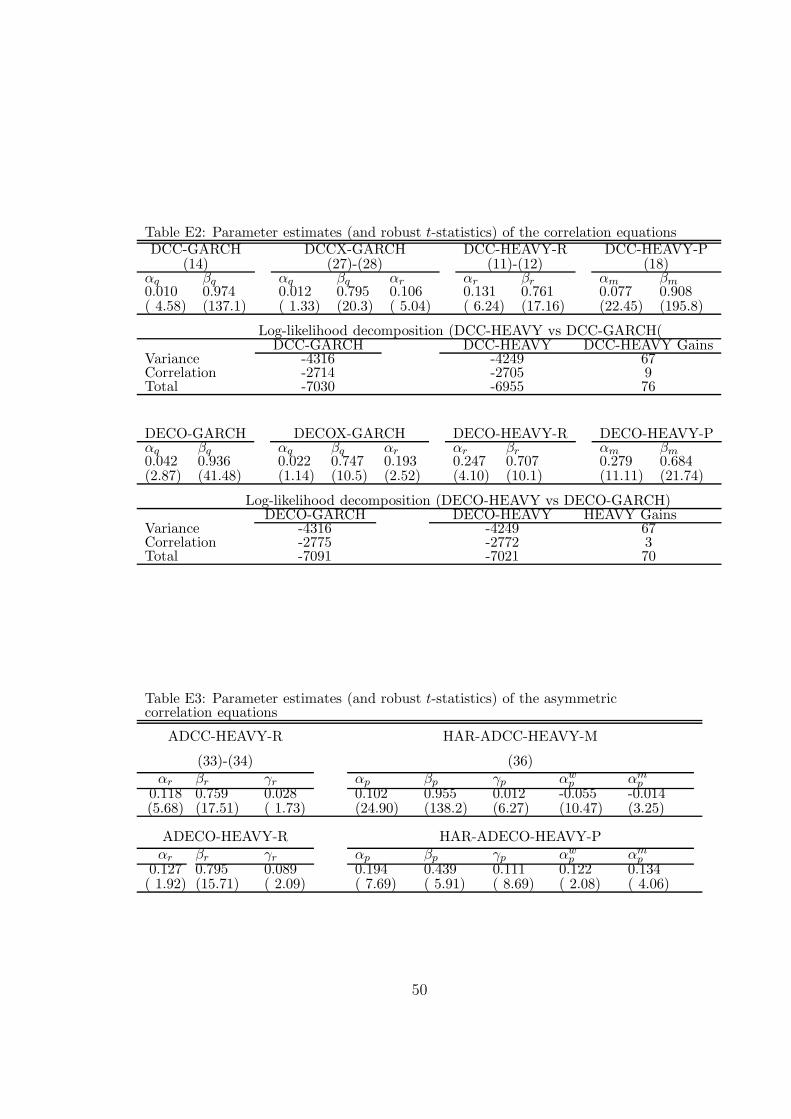
Tables E1 (variance equations) and E2 (correlation equations) show the full sampleestimation results. The results are broadly similar to those reported in Section 5.2.As shown by the reported maximum and minimum values in Table C1 (compared tothe values in Table 1), there is less heterogeneity between the parameter estimates ofthe variance equations for the 10 stocks of the NSS data than for the 29 stocks, whichis not surprising given the smaller number of stocks and their selection criterion.Nevertheless, the median values of both sets of estimates are very similar.
For the correlation equations, a comparison with the estimates reported in TablesC2 and 2) does not reveal important differences. The higher t-statistics for the 29stocks are due to the larger sample size.
Table E3 (comparable to Table 6 for the 29 stocks) shows the estimates of theasymmetric correlation equations, with HAR terms in the realized correlation part(HEAVY-M). The estimates of the coefficients of the asymmetric terms ((γr and γp)are similar, except for the ADECO-HEAVY-R, where the estimate of γr is positiveand significant for the NSS dataset. For the HAR terms, the estimates for the tenstocks are larger in absolute value; notice that αw
p and αmp are both estimated to be
significantly negative in the HAR-ADCC-HEAVY-M.
48
Table E1: Parameter estimates (and robust t-statistics) of the variance equations
For out-of-sample forecast results, the models are estimated on rolling windows of1486 observations, resulting in a total of 756 forecasts for s = 1, 752 for s = 5, and735 for s = 22. The first rolling window is chosen such that forecasts start on 3January 2007. The last forecast is for 31 December 2009.
Tables C4 to C8 present the results in the same way as the Tables 3-5 and 7-8for the 29 stocks. A few comments follow.
1) MCS99 for covariance forecasts (Table C4 compared to Table 3): the main dif-ference is the inclusion in the MCS99 of the BEKK-HEAVY model at the threehorizons and for all loss functions. A possible explanation for this is the differencein the number of stocks between the two datasets: the flexibility of DCC with respectto BEKK is more important for 29 stocks than for 10 (the most liquid ones).
Another difference is that the MCS99 include more models than for the 29 stocks.Nevertheless, the results are clearly in favour of HEAVY models: GARCH modelsare included in MCS99 only at horizon 22 and for the QLIK and MV loss functions.This is reflected in the Covariance panels of Tables C6-C8 where only three ratios(for QLIK loss) are marginally larger than one, whereas the other ratios are all belowone; the improvements are important especially for FN loss.
2) MCS99 for correlation forecasts (Table C5 compared to Table 4, Correlation pan-els): for FN loss, few differences; for QLIK loss, some GARCH models (dependingon the horizon) belong to the MCS99, in addition to several HEAVY models. Theratios in the Correlation panels of Tables C6-C8 are in a majority of cases (27 outof 36) smaller than one, but not much (the smallest being 0.914); the 10 ratiosthat exceed one are very close to one (the largest being 1.031). In brief, even if theHEAVY models do improve correlation forecasts, this is not strongly and some DCCand DECO models do as well.
3) MCS99 for variance forecasts (Table C5 compared to Table 4, Variance panels):When comparing all models, DCC-HEAVY and ADCC-HEAVY are in the MCS99for both loss functions and all horizons (with one exception for DCC-HEAVY).Their values of their loss functions are close. Loss ratios show that the GARCHmodels (DCC and ADCC) are dominated by the HEAVY models, even if DCC isin the three MCS99 for MSE loss. The advantage of HEAVY over GARCH modelsdecreases as s increases.
51
Table E4: MCS for loss functions of out-of-sample covariance forecastingFN MCS QLIK MCS GMV MCS MV MCS
Values of loss functions in bold identify the models in the 99% level MCS when thecomparison is limited to the first six models. Underlined values identify the models inthe 99% level MCS when the comparison is done for all models. A value in bold but notunderlined is thus in the MCS of the first six models, but is excluded when consideringall models. The MCS rankings are for the global comparison.
52
Table E5: MCS for loss functions of out-of-sample correlation and variance forecasting
Values of loss functions in bold identify the models in the 99% level MCS when the com-parison is limited to the first six models. Underlined values identify the models in the 99%level MCS when the comparison is done for all models. A value in bold but not underlinedis thus in the MCS of the first six models, but is excluded when considering all models.The MCS rankings are for the global comparison.
53
Table E6: Out-of-sample loss ratios between DCC-HEAVY and DCC-GARCH