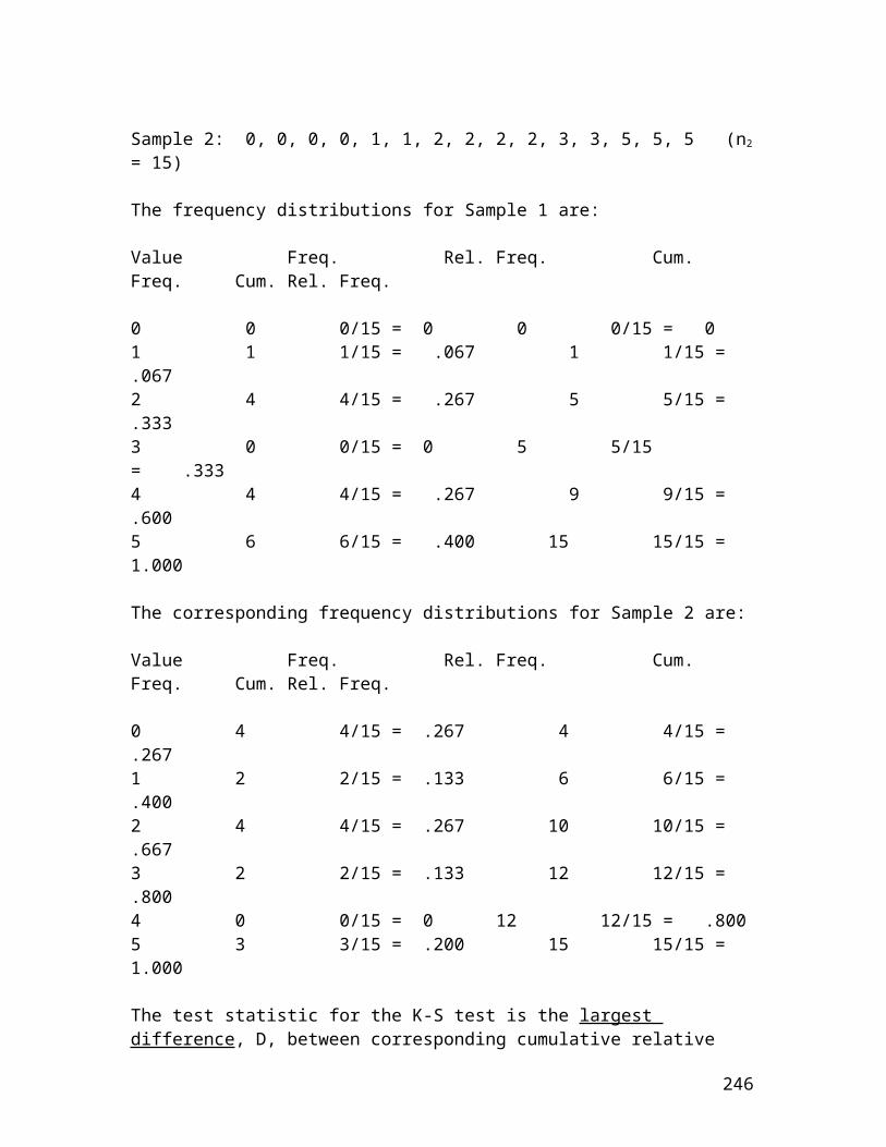
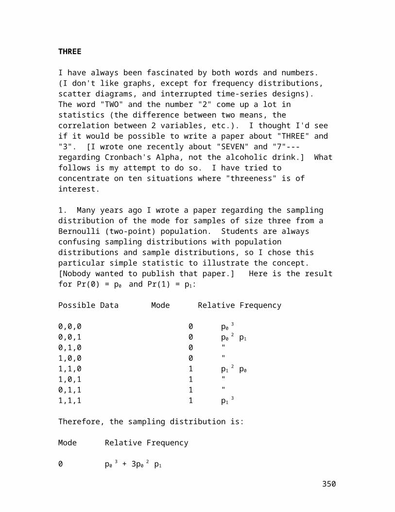
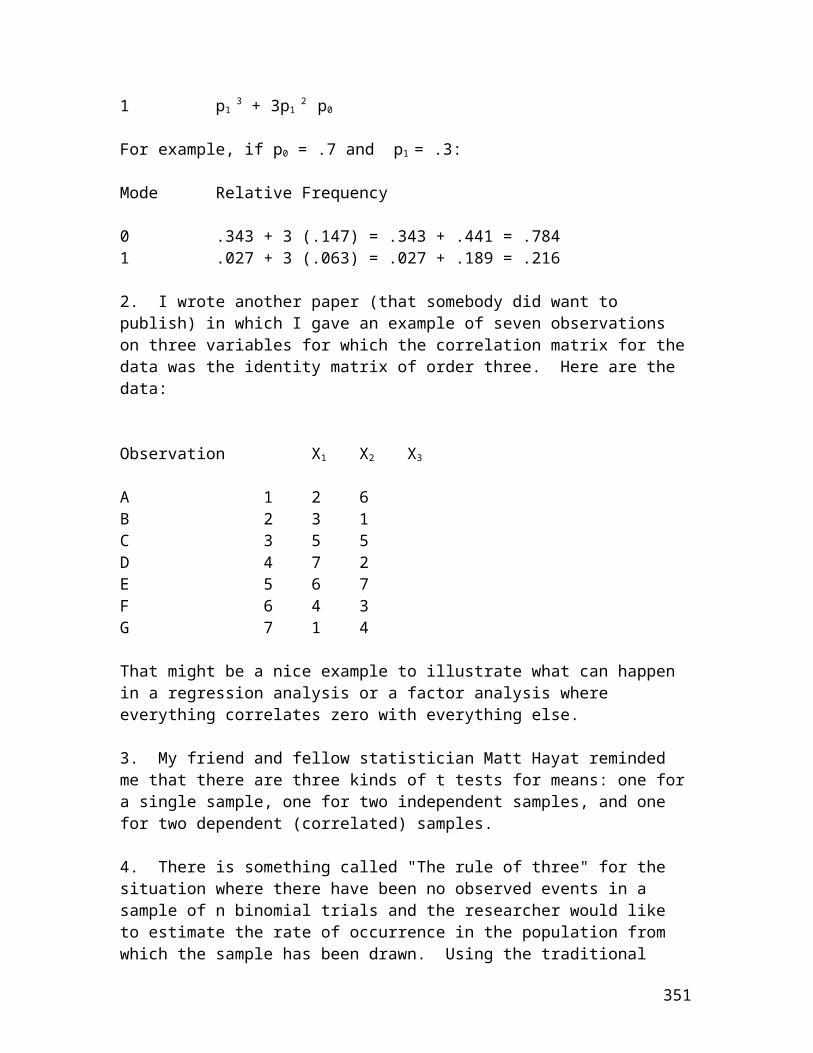
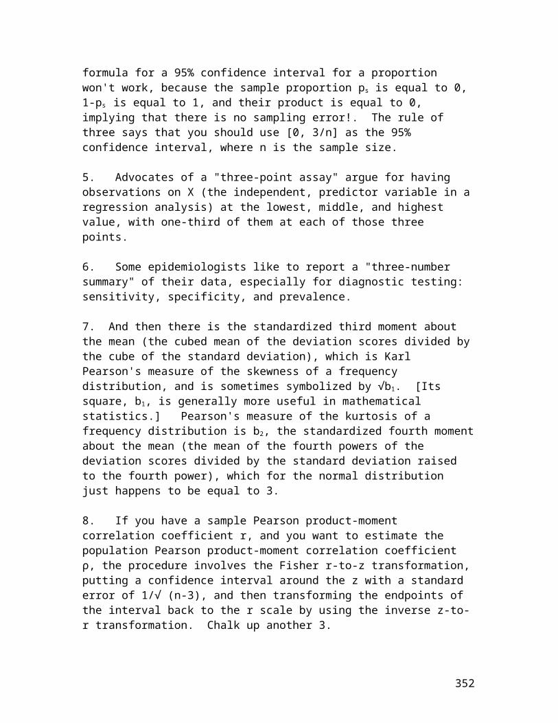
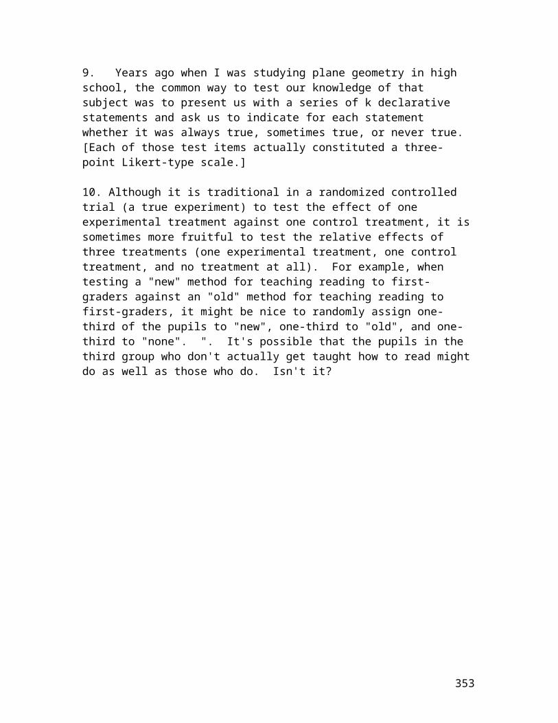
In this document I have tried to put together a number of unpublished papers I wrote during the last several years. They range in length from 3 pages to 90 pages, and in complexity from easy to fairly technical. The papers are inrough chronological order, from 2004 until 2014. I think there's something in here for everybody. Feel free to download and/or print anything that you find to be of interest. Enjoy!
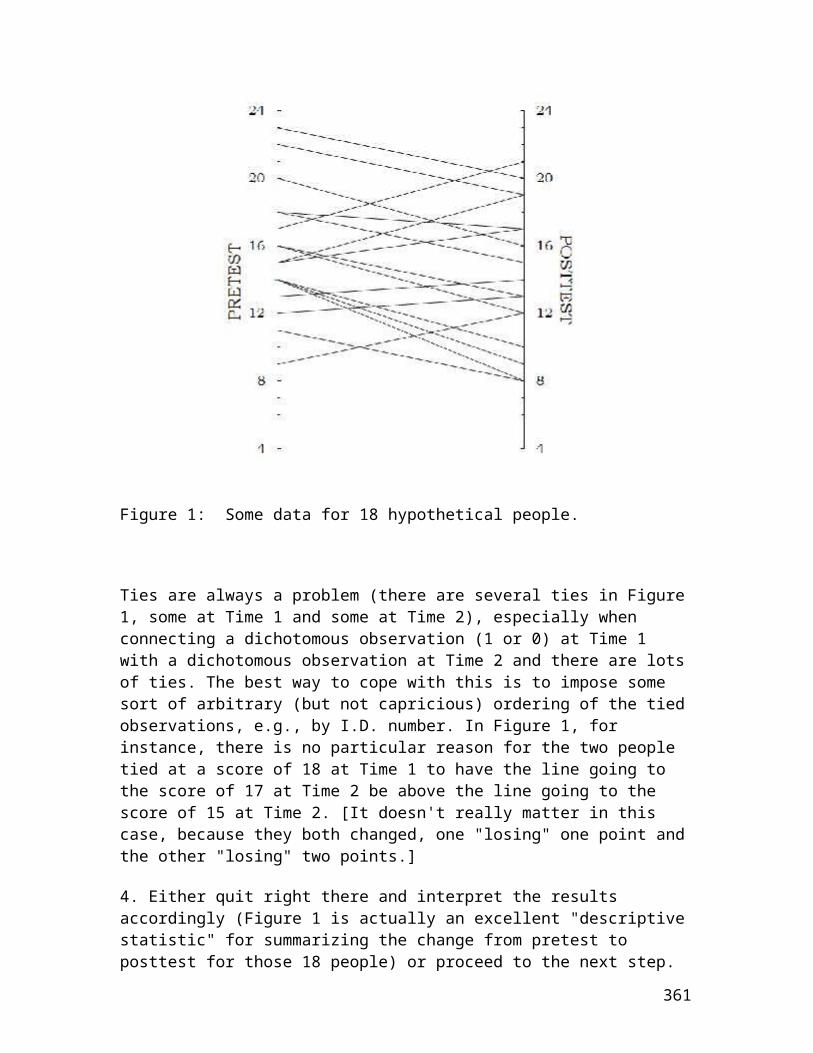
Table of Contents
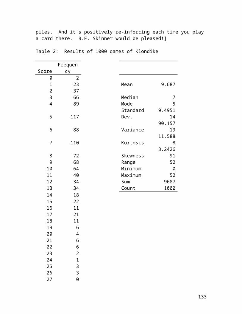
Investigating the relationship between two variables...........................................3
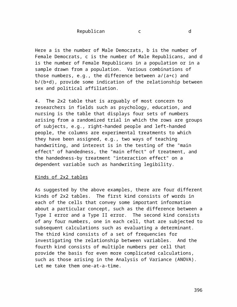
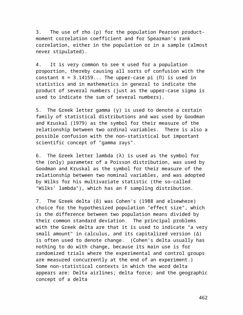
Minus vs. divided by...........................................................................................19
Percentages: The most useful statistics ever invented.....................................26
Significance test, confidence interval, both, or neither? ..................................116
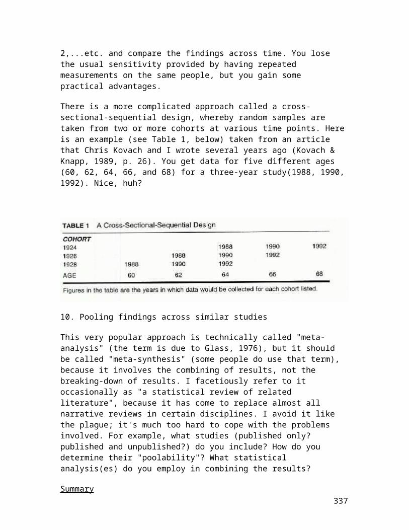
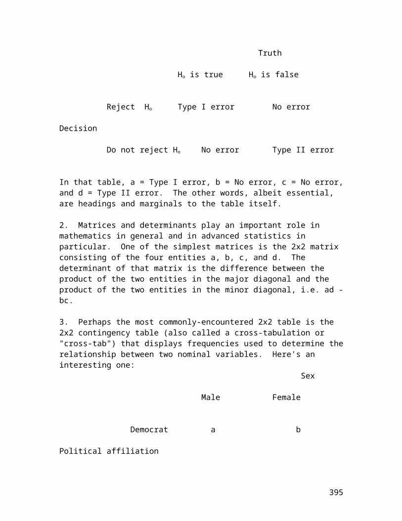
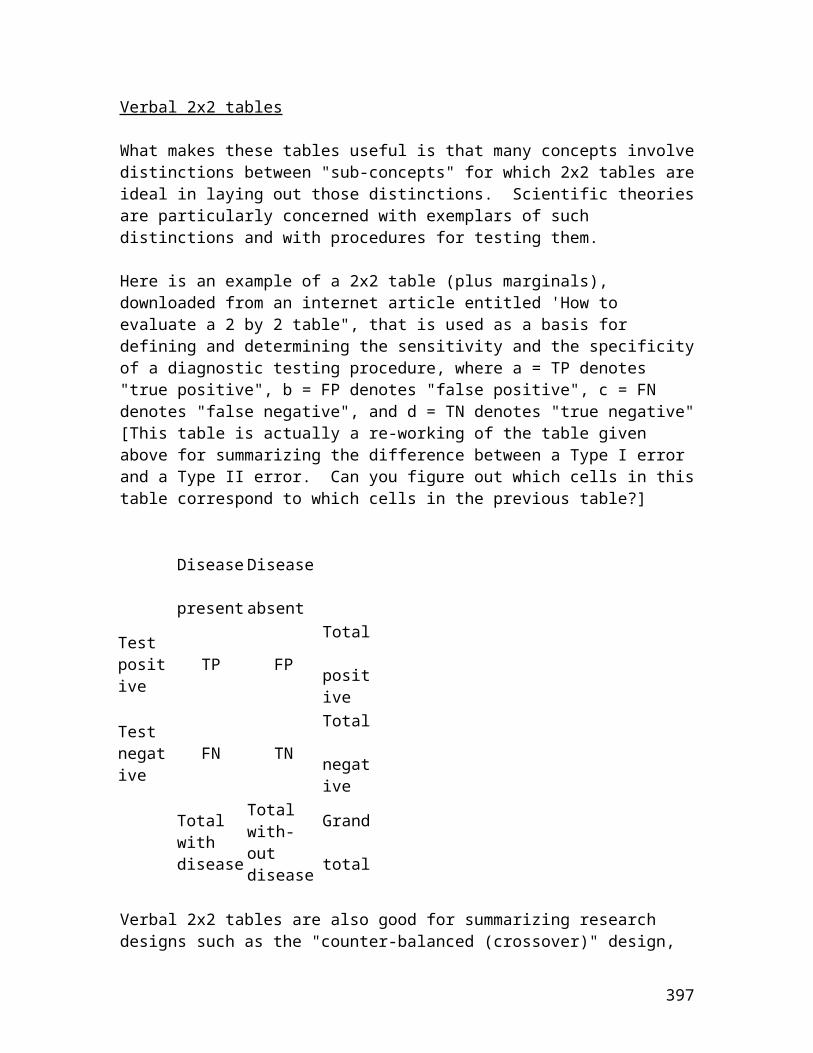
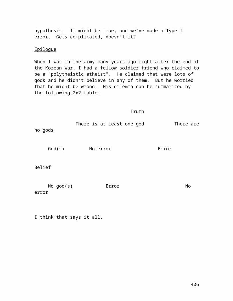
INVESTIGATING THE RELATIONSHIP BETWEEN TWO VARIABLES
Abstract
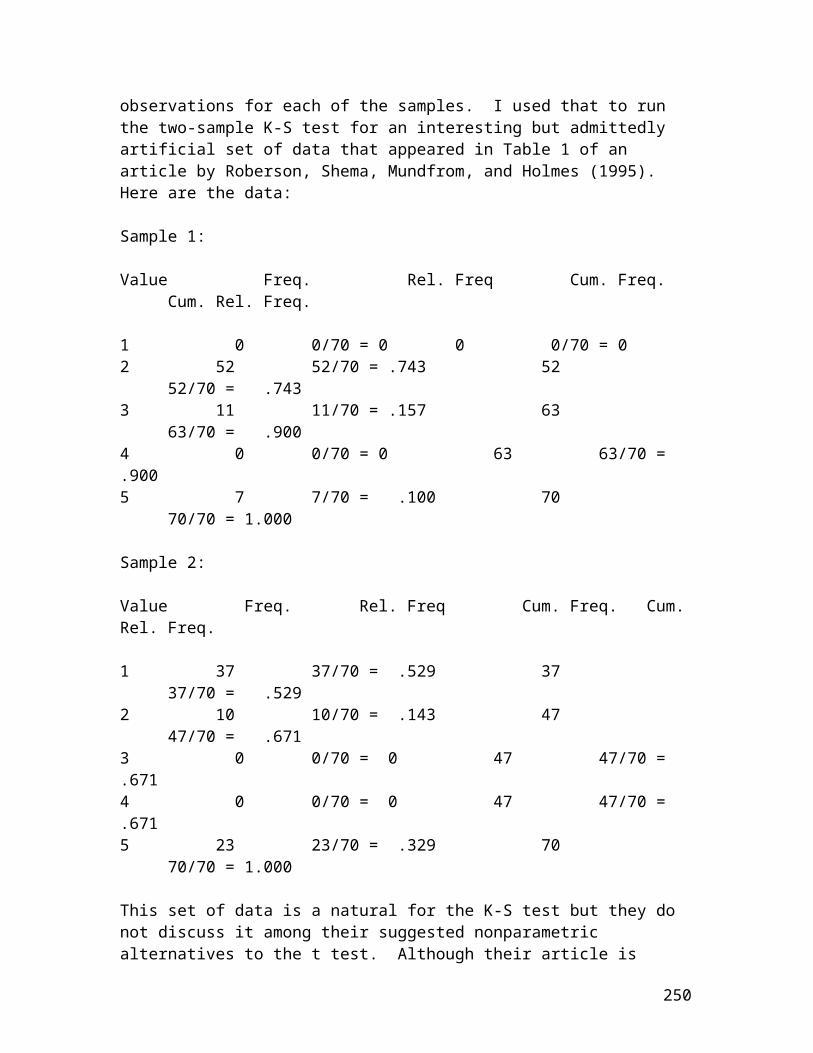
"What is the relationship between X and Y?", where X is one variable, e.g., height, and Y is another variable, e.g., weight, is one of the most common research questions in all of the sciences. But what do we mean by "the relationship between two variables"? Why do we investigate such relationships? How do we investigate them? How do we display the data? How do we summarize the data? And how do we interpret the results? In this paper I discuss various approaches that have been taken, including some of the strengths and weaknesses of each.
The ubiquitous research question
"What is the relationship between X and Y?" is, and always has been, a question of paramount interest to virtually all researchers. X and Y might be different forms of a measuring instrument. X might be a demographic variable such as sex or age, and Y might be a socioeconomic variable such as education or income. X might be an experimentally manipulable variable such as drug dosage and Y might be an outcome variable such as survival. The list goes on and on.But why are researchers interested in that question? There are at least three principal reasons:
1. Substitution. If there is a strong relationship betweenX and Y, X might be substituted for Y, particularly if X is less expensive in terms of money, time, etc. The first example in the preceding paragraph is a good illustration ofthis reason; X might be a measurement of height taken with atape measure and Y might be a measurement of height taken with an electronic stadiometer.
2. Prediction. If there is a strong relationship between Xand Y, X might be used to predict Y. An equation for
4
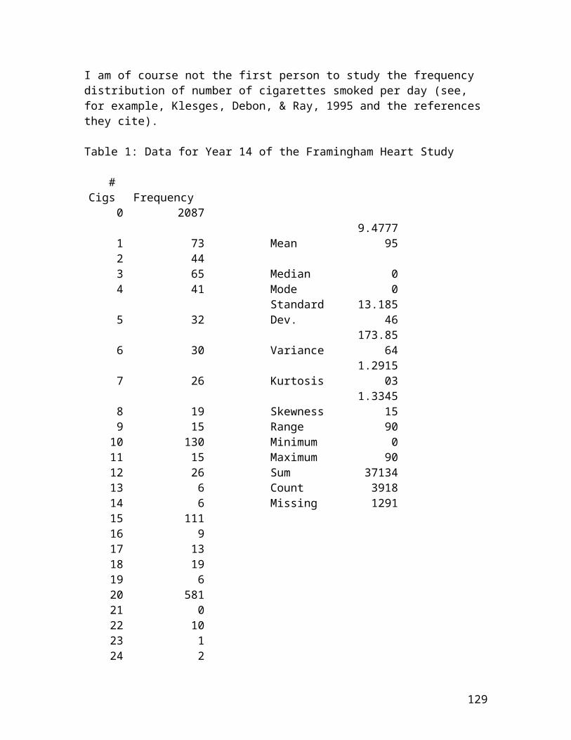
predicting income (Y) from age (X) might be helpful in understanding the trajectory in personal income across the age span.
3. Causation. If there is a strong relationship between X and Y, and other variables are directly or statistically controlled, there might be a solid basis for claiming, for example, that an increase in drug dosage causes an increase in life expectancy.
What does it mean?
In a recent internet posting, Donald Macnaughton (2002) summarized the discussion that he had with Jan deLeeuw, Herman Rubin, and Robert Frick regarding seven definitions of the term "relationship between variables". The seven definitions differed in various technical respects. My personal preference is for their #6:
There is a relationship between the variables X and Y if, for at least one pair of values X' and X" of X, E(Y|X') ~= E(Y|X"), where E is the expected-value operator, the vertical line means "given", and ~= means "is not equal to".(It indicates that X varies, Y varies, and all of the X's are not associated with the same Y.)
Research design
In order to address research questions of the "What is the relationship between X and Y?" type, a study must be designed in a way that will be appropriate for providing thedesired information. For relationship questions of a causalnature a double-blind true experimental design, with simple random sampling of a population and simple random assignmentto treatment conditions, might be optimal. For questions concerned solely with prediction, a survey based upon a stratified random sampling design is often employed. And ifthe objective is to investigate the extent to which X might be substituted for Y, X must be "parallel" to Y (a priori
5
comparably valid, with measurements on the same scale so that degree of agreement as well as degree of association can be determined).
Displaying the data
For small samples the raw data can be listed in their entirety in three columns: one for some sort of identifier; one for the obtained values for X; and one for the corresponding obtained values for Y. If X and Y are both continuous variables, a scatterplot of Y against X should be used in addition to or instead of that three-column list.[An interesting alternative to the scatterplot is the "pair-link" diagram used by Stanley (1964) and by Campbell and Kenny (1999) to connect corresponding X and Y scores.] If Xis a categorical independent variable, e.g., type of treatment to which randomly assigned in a true experiment, and Y is a continuous dependent variable, a scatterplot is also appropriate, with values of X on the horizontal axis and with values of Y on the vertical axis.
For large samples a list of the raw data would usually be unmanageable, and the scatterplot might be difficult to display with even the most sophisticated statistical software because of coincident or approximately coincident data points. (See, for example, Cleveland, 1995; Wilkinson,2001.) If X and Y are both naturally continuous and the sample is large, some precision might have to be sacrificed by displaying the data according to intervals of X and Y in a two-way frequency contingency table (cross-tabulation). Such tables are also the method of choice for categorical variables for large samples.
How small is small and how large is large? That decision must be made by each individual researcher. If a list of the raw data gets to be too cumbersome, if the scatterplot gets too cluttered, or if cost considerations such as the amount of space that can be devoted to displaying the data come into play, the sample can be considered large.
6
Summarizing the data
For continuous variables it is conventional to compute the means and standard deviations of X and Y separately, the Pearson product-moment correlation coefficient between X andY, and the corresponding regression equation(s), if the objective is to determine the direction and the magnitude ofthe degree of linear relationship between the two variables.Other statistics such as the medians and the ranges of X andY, the residuals (the differences between the actual values of Y and the values of Y on the regression line for the various values of X), and the like, might also be of interest. If curvilinear relationship is of equal or greater concern, the fitting of a quadratic or exponential function might be considered.
[Note: There are several ways to calculate Pearson's r, allof which are mathematically equivalent. Rodgers & Nicewander (1988) provided thirteen of them. There are actually more than thirteen. I derived a rather strange-looking one several years prior to that (Knapp, 1979) in an article on estimating covariances using the incidence sampling technique developed by Sirotnik & Wellington (1974).]
For categorical variables there is a wide variety of choices. If X and Y are both ordinal variables with a smallnumber of categories (e.g., for Likert-type scales), Goodmanand Kruskal's (1979) gamma is an appropriate statistic. If the data are already in the form of ranks or easily convertible into ranks, one or more rank-correlation coefficients, e.g., Spearman's rho or Kendall's tau, might be preferable for summarizing the direction and the strengthof the relationship between the two variables.
If X and Y are both nominal variables, indexes such as the phi coefficient (which is mathematically equivalent to Pearson's r for dichotomous variables) or Goodman and
7
Kruskal's (1979) lambda might be equally defensible alternatives.
For more on displaying data in contingency tables and for the summarization of such data, see Simon (1978) and Knapp (1999).
Interpreting the data
Determining whether or not a relationship is strong or weak,statistically significant or not, etc. is part art and part science. If the data are for a full population or for a "convenience" sample, no matter what size it may be, the interpretation should be restricted to an "eyeballing" of the scatterplot or contingency table, and the descriptive (summary) statistics . For a probability sample, e.g., a simple random random or a stratified random sample, statistical significance tests and/or confidence intervals are usually required for proper interpretation of the findings, as far as any inference from sample to population is concerned. But sample size must be seriously taken into account for those procedures or anomalous results could arise, such as a statistically significant relationship thatis substantively inconsequential. (Careful attention to choice of sample size in the design phase of the study should alleviate most if not all of such problems.)
An example
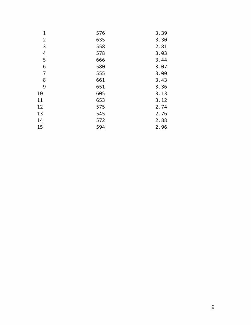
The following example has been analyzed and scrutinized by many researchers. It is due to Brad Efron and his colleagues (see, for example, Diaconis & Efron, 1983). [LSAT = Law School Aptitude Test; GPA = Grade Point Average]
Data display(s)
Law School Average LSAT score Average Undergraduate GPA
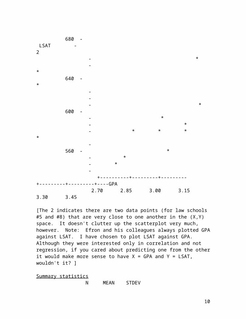
[The 2 indicates there are two data points (for law schools #5 and #8) that are very close to one another in the (X,Y) space. It doesn't clutter up the scatterplot very much, however. Note: Efron and his colleagues always plotted GPAagainst LSAT. I have chosen to plot LSAT against GPA. Although they were interested only in correlation and not regression, if you cared about predicting one from the otherit would make more sense to have X = GPA and Y = LSAT, wouldn't it? ]
Summary statistics N MEAN STDEV
10
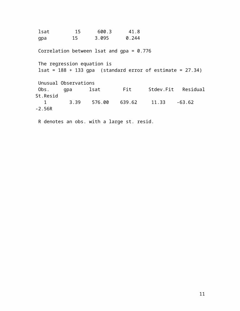
lsat 15 600.3 41.8 gpa 15 3.095 0.244 Correlation between lsat and gpa = 0.776 The regression equation is lsat = 188 + 133 gpa (standard error of estimate = 27.34) Unusual Observations Obs. gpa lsat Fit Stdev.Fit ResidualSt.Resid 1 3.39 576.00 639.62 11.33 -63.62 -2.56R R denotes an obs. with a large st. resid.
11
Interpretation
The scatterplot looks linear and the correlation is rather high (it would be even higher without the outlier). Prediction of average LSAT from average GPA should be generally good, but could be off by about 50 points or so (approximately two standard errors of estimate).
If this sample of 15 law schools were to be "regarded" as a simple random sample of all law schools, a statistical inference might be warranted. The correlation coefficient of .776 for n = 15 is statistically significant at the .05 level, using Fisher's r-to-z transformation; and the 95% confidence interval for the population correlation extends from .437 to .922 on the r scale (see Knapp, Noblitt, & Viragoontavan, 2000), so we can be reasonably assured that in the population of law schools there is a non-zero linear relationship between average LSAT and average GPA.
Complications
Although that example appears to be simple and straightforward, it is actually rather complicated, as are many other two-variable examples. Here are some of the complications and some of the ways to cope with them:
1. Scaling. It could be argued that neither LSAT nor GPA are continuous, interval-level variables. The LSAT score onthe 200-800 scale is usually determined by means of a non-linear normalized transformation of a raw score that might have been corrected for guessing, using the formula number of right answers minus some fraction of the number of wrong answers. GPA is a weighted heterogeneous amalgam of course grades and credit hours where an A is arbitrarily given 4 points, a B is given 3 points, etc. It might be advisable, therefore, to rank-order both variables and determine the rank correlation between the corresponding rankings. Spearman's rho for the ranks is .796 (a bit higher than the Pearson correlation between the scores).
12
2. Weighting. Each of the 15 law schools is given a weightof 1 in the data and in the scatterplot. It might be preferable to assign differential weights to the schools in accordance with the number of observations that contribute to its average, thus giving greater weight to the larger schools. Korn and Graubard (1998) discuss some very creative ways to display weighted observations in a scatterplot.
3. Unit-of analysis. The sample is a sample of schools, not students. The relationship between two variables such as LSAT and GPA that is usually of principal interest is therelationship that would hold for individual persons, not aggregates of persons, and even there one might have to choose whether to investigate the relationship within schoolor across schools. The unit-of-analysis problem has been studied for many years (see, for example, Robinson, 1950 andKnapp, 1977), and has been the subject of several books and articles, more recently under the heading "hierarchical linear modeling" rather than "unit of analysis" (see, for example, Raudenbush & Bryk, 2002 and Osborne, 2000).
4. Statistical assumptions. There is no indication that those15 schools were drawn at random from the population of all law schools, and even if they were, a finite population correction should be applied to the formulas for the standard errors used in hypothesis testing or interval estimation, since the population at the time (the data were gathered in 1973) consisted of only 82 schools, and 15 schools takes too much of a "bite" out of the 82.
Fisher's r-to-z transformation only "works" for a bivariate normal population distribution. Although the scatterplot for the 15 sampled schools looks approximately bivariate normal, that may not be the case in the population, so a conservative approach to the inference problem would involvea choice of one or more of the following approaches:
13
a. A test of statistical significance and/or an interval estimate for the rank correlation. Like the correlation of .776 between the scores, the rank correlation of .796 is also statistically significant at the .05 level, but the confidence interval for the population rank correlation is shifted to the right and is slightly tighter.
b. Application of the jackknife to the 15 bivariate observations. Knapp, et al. (2000) did that for the "leave one out" jackknife and estimated the 95% confidence intervalto be from approximately .50 to approximately .99.
c. Application of the bootstrap to those observations. Knapp, et al. (2000) did that also [as many other researchers, including Diaconis & Efron, 1983 had done], andthey found that the middle 95% of the bootstrapped correlations ranged from approximately .25 to approximately .99.
d. A Monte Carlo simulation study. Various population distributions could be sampled, the resulting estimates of the sampling error for samples of size 15 from those populations could be determined, and the corresponding significance tests and/or confidence intervals carried out. One population distribution that might be considered is the bivariate exponential.
5. Attenuation. The correlation coefficient of .776 is thecorrelation between obtained average LSAT score and obtainedaverage GPA at those 15 schools. Should the relationship ofinterest be an estimate of the correlation between the corresponding true scores rather than the correlation between the obtained scores? It follows from classical measurement theory that the mean true score is equal to the mean obtained score, so this should not be a problem with the given data, but if the data were disaggregated to the individual level a correction for attenuation (unreliability) may be called for. (See, for example, Muchinsky, 1996 and Raju & Brand, 2003; the latter article
14
provides a significance test for attenuation-corrected correlations.) It would be relatively straightforward for LSAT scores, since the developers of that test must have some evidence regarding the reliability of the instrument. But GPA is a different story. Has anyone ever investigated the reliability of GPA? What kind of reliability coefficient would be appropriate? Wouldn't it be necessary to know something about the reliability of the classroom tests and the subsequent grades that "fed into" the GPA?
6. Restriction of range. The mere fact that the data are average scores presents a restriction-of-range problem, since average scores vary less from one another than individual test scores do. There is also undoubtedly an additional restriction because students who apply to law schools and get admitted have (or should have) higher LSAT scores and higher GPAs than students in general. A correction for restriction of range to the correlation of .776 might be warranted (the end result of which should be an even higher correlation), and a significance test is also available for range-corrected correlations (Raju & Brand, 2003).
7. Association vs. agreement. Reference was made above to the matter of association and agreement for parallel forms of measuring instruments. X and Y could be perfectly correlated (for example, X = 1,2,3,4,5, and Y = 10,20,30,40,50, respectively) but not agree very well in anyabsolute sense. That is irrelevant for the law school example, since LSAT and GPA are not on the same scale, but for many variables it is the matter of agreement in additionto the matter of association, that is of principal concern (see, for example, Robinson, 1957 and Engstrom, 1988).
8. Interclass vs. intraclass. If X and Y are on the same scale, Fisher's (1958) intraclass correlation coefficient may be more appropriate than Pearson's product-moment correlation coefficient (which Fisher called an interclass correlation). Again this is not relevant for the law school
15
example, but for some applications, e.g., an investigation of the relationship between the heights of twin-pairs, Pearson's r would actually be indeterminate because we wouldn't know which height to put in which column for a given twin-pair.
9. Precision. How many significant digits or decimal places are warranted when relationship statistics such as Pearson r's are reported? Likewise for the p-values or confidence coefficients that are associated with statisticalinferences regarding the coresponding population parameters.For the law school example I reported an r of .776, a p of (less than) .05, and a 95% confidence interval. Should I have been more precise and said that r = .7764 or less precise and said that r = .78? The p that "goes with" an r of .776 is actually closer to .01 than to .05. And would anybody care about a confidence coefficient of, say, 91.3?
10. Covariance vs. correlation. Previous reference was made to the tradition of calculating Pearson's r for two continuous variables whose linear relationship is of concern. In certain situations it might be preferable to calculate the scale-bound covariance between X and Y rather than, or in addition to, the scale-free correlation. In structural equation modeling it is the covariances, not the correlations, that get analyzed. And in hierarchical linearmodeling the between-aggregate and within-aggregate covariances sum to the total covariance, but the between-aggregate and within-aggregate correlations do not (see Knapp, 1977).
Another example
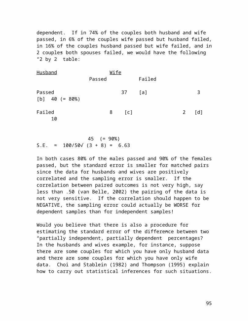
The following table (from Agresti, 1990) summarizes responses of 91 married couples to a questionnaire item. This example has also been analyzed and scrutinized by many people [perhaps because of its prurient interest?].
16
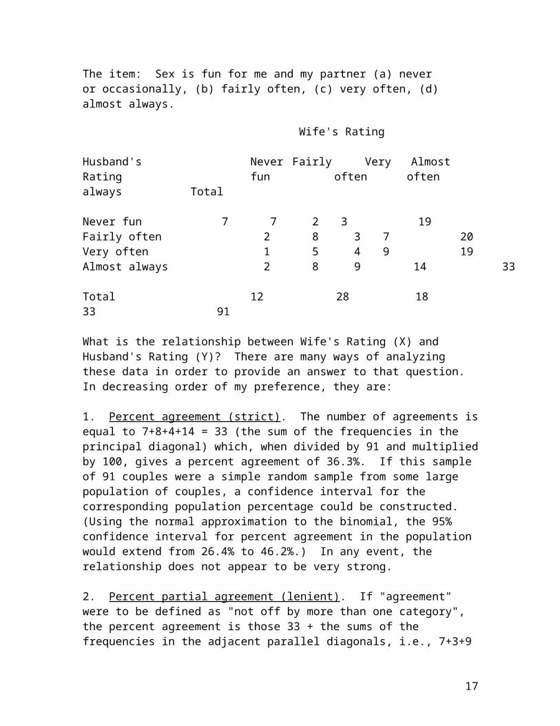
The item: Sex is fun for me and my partner (a) never or occasionally, (b) fairly often, (c) very often, (d) almost always.
Wife's Rating
Husband's Never Fairly Very AlmostRating fun often often always Total
Never fun 7 7 2 3 19Fairly often 2 8 3 7 20Very often 1 5 4 9 19Almost always 2 8 9 14 33
Total 12 28 18 33 91
What is the relationship between Wife's Rating (X) and Husband's Rating (Y)? There are many ways of analyzing these data in order to provide an answer to that question. In decreasing order of my preference, they are:
1. Percent agreement (strict). The number of agreements isequal to 7+8+4+14 = 33 (the sum of the frequencies in the principal diagonal) which, when divided by 91 and multipliedby 100, gives a percent agreement of 36.3%. If this sample of 91 couples were a simple random sample from some large population of couples, a confidence interval for the corresponding population percentage could be constructed. (Using the normal approximation to the binomial, the 95% confidence interval for percent agreement in the population would extend from 26.4% to 46.2%.) In any event, the relationship does not appear to be very strong.
2. Percent partial agreement (lenient). If "agreement" were to be defined as "not off by more than one category", the percent agreement is those 33 + the sums of the frequencies in the adjacent parallel diagonals, i.e., 7+3+9
17
= 19 and 2+5+9 = 16, for a total of 68 "agreements" out of 91 possibilities, or 74.7%.
3. Goodman and Kruskal's (1979) gamma. The two variables are both ordinal (percent agreement does not take advantage of that ordinality, but it is otherwise very simple and veryattractive) and the number of categories is small (4), so byapplying any one of the mathematically-equivalent formulas for gamma, we have gamma = .047.
4. Goodman and Kruskal's (1979) lambda. Not as good a choice as Goodman's gamma, because it does not reflect the ordinality of the two variables. For these data lambda = .159.
5. Somers' (1962) D. Somers' D is to be preferred to gammaif the two variables take on independent and dependent roles(for example, if we would like to predict husband's rating from wife's rating, or wife's rating from husband's rating).That does not appear to be the case here, but Somers' D for these data is .005.
6. Cohen's (1960) kappa. This is one of my least favorite statistics, since it incorporates a "correction" to percent agreement for chance agreements and I don't believe that people ever make chance ratings. But it is extremely popular in certain disciplines (e.g., psychology) and some people would argue that it would be appropriate for the wife/husband data, for which it is .129 (according to the graphpad.com website calculator and Michael Friendly's website). ["Weighted kappa", a statistic that reflects partial agreement, also "corrected for chance", is .237.] The sampling distribution of Cohen's kappa is a mess (see, for example, Fleiss, Cohen, & Everitt, 1969), but the graphpad.com calculator yielded a 95% confidence interval of-.006 to .264 for the population unweighted kappa.
7. Krippendorff's (1980) alpha . This statistic is allegedto be an improvement over Cohen's kappa, since it also
18
"corrects" for chance agreements and is a function of both agreements and disagreements. For these data it is .130. (See the webpage entitled "Computing Krippendorff's Alpha-Reliability".) "Alpha" is a bad choice for the name of this statistic, since it can be easily confused with Cronbach's (1951) alpha.
8. Contingency coefficient. Not recommended; it also does not reflect ordinality and its range is not from the usually-desirable -1 to +1 or 0 to +1.
9. Rank correlation. Not recommended; there are too many "ties".
10. Pearson's r. Also not recommended; it would treat the two variables as interval-level, which they definitely are not. [I would guess, however, that over half of you would have done just that!]
A third (and final) example
One of the most common research contexts is a true experiment in which each subject is randomly assigned to an experimental group or to a control group and the two groups are compared on some continuous variable in order to determine whether or not, or the extent to which, the treatment as operationalized in the experimental condition has had an effect. Here X is a dichotomous (1, 0) nominal independent variable and Y is a continuous dependent variable. An example of such a context was provided by Dretzke (2001) in her book on the use of Excel for statistical analyses:
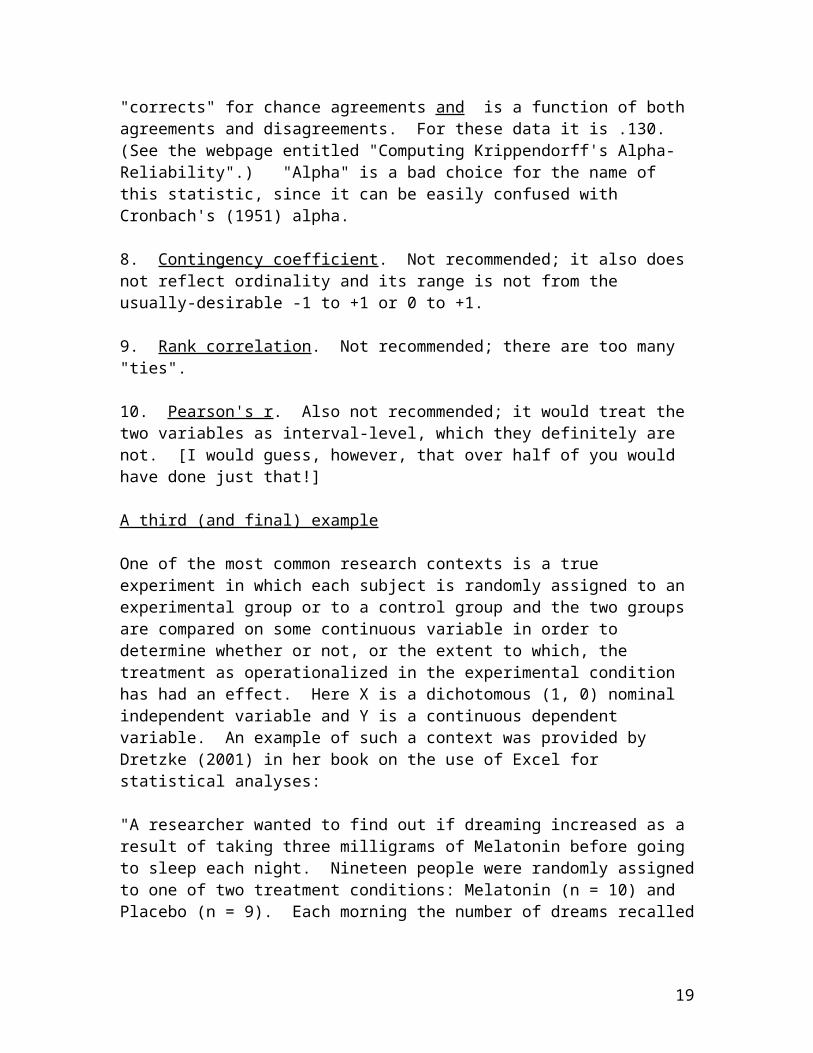
"A researcher wanted to find out if dreaming increased as a result of taking three milligrams of Melatonin before going to sleep each night. Nineteen people were randomly assignedto one of two treatment conditions: Melatonin (n = 10) and Placebo (n = 9). Each morning the number of dreams recalled
19
were reported and tallied over a one-week period. " (p. 152)
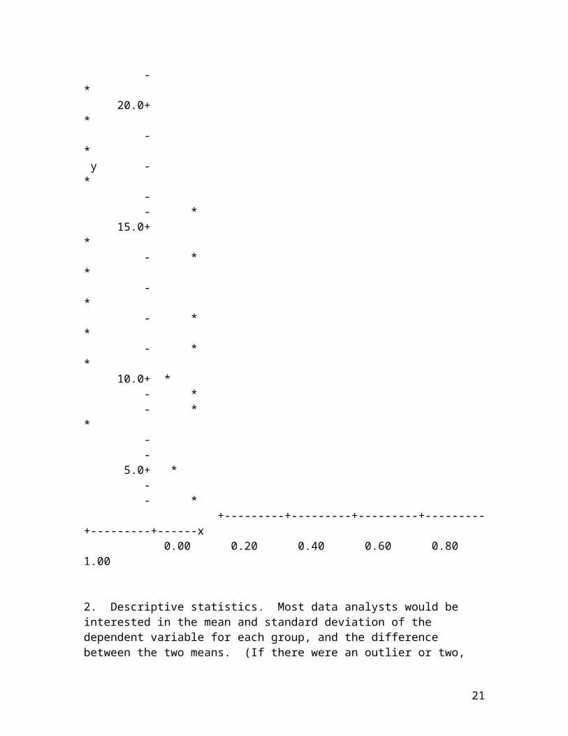
1. Displaying the data. The listing of the 19 "scores" on the dependent variable in two columns (without identifiers), with 10 of the scores under the "Melatonin" column (experimental group) and 9 of the scores under the "Placebo" column (control group) seems at least necessary ifnot sufficient. It might be advisable to re-order the scores in each column from high to low or from low to high, however, and/or display the data graphically, as follows:
20
- * 20.0+ * - * y - * - - * 15.0+ * - * * - * - * * - * * 10.0+ * - * - * * - - 5.0+ * - - * +---------+---------+---------+---------+---------+------x 0.00 0.20 0.40 0.60 0.80 1.00 2. Descriptive statistics. Most data analysts would be interested in the mean and standard deviation of the dependent variable for each group, and the difference between the two means. (If there were an outlier or two,
21
the medians and the ranges might be preferred instead of, orin addition to, the means and standard deviations.) And since the relationship between the two variables (X = type of treatment and Y = number of dreams recalled) is of primary concern, the point-biserial correlation between X and Y (another special case of Pearson's r) should also be calculated. For the given data those summary statistics are:
Melatonin: mean = 15.1; standard deviation = 4.3 (median = 14.5; range = 13)
Placebo: mean = 9.8; standard deviation = 4.1 (median = 10.0; range = 13)
Difference between the means = 15.1 - 9.8 = 5.3
Correlation between X (type of treatment) and Y (number of dreams recalled) = .56 (with the Melatonin group coded 1 andthe Placebo group coded 0)
3. Inferential statistics. Almost everyone would carry outa two independent samples one-tailed t test. That would be inadvisable, however, for a number of reasons. First of all, although the subjects were randomly assigned to treatments there is no indication that they were randomly sampled. [See the opposing views of Levin, 1993 and Shaver,1993 regarding this distinction. Random sampling, not random assignment, is one of the assumptions underlying the t test. ] Secondly, the t test assumes that in the populations from which the observations were drawn the distributions are normal and homoscedastic (equal spread). Since there is apparently only one population that has been sampled (and that not randomly sampled) and its distributionis of unknown shape, that is another strike against the t test. (The sample observations actually look like they've been sampled from rectangular, i.e., uniform, distributions and the two samples have very similar variability, but that
22
doesn't really matter; it's what's going on in the population that counts.)
The appropriate inferential analysis is a randomization test(sometimes called a permutation test)--see, for example, Edgington (1995)--where the way the scores (number of dreamsrecalled) happened to fall into the two groups subsequent tothe particular randomization employed is compared to all of the possible ways that they could have fallen, under the null hypothesis that the treatments are equally effective and the Melatonin group would always consist of 10 people and the Placebo group would always consist of 9 people. [Ifthe null hypothesis were perfectly true, each person would recall the same number of dreams no matter which treatment he/she were assigned to.] The number of possible ways is equal to the number of combinations of 19 things taken 10 ata time (for the number of different allocations to the experimental group; the other 9 would automatically comprisethe control group), which is equal to 92378, a very large number indeed. As an example, one of the possible ways would result in the same data as above but with the 21 and the 3 "switched". For that case the Melatonin mean would be13.3 and the Placebo mean would be 11.8, with a corresponding point biserial correlation of .16 between typeof treatment and number of dreams recalled.
I asked John Pezzullo [be sure to visit his website some time, particularly the Interactive Stats section] to run theone-tailed randomization test for me. He very graciously did so and obtained a p-value of .008 (the difference between the two means is statistically significant at the .01 level) and so it looks like the Melatonin was effective (if it's good to be able to recall more dreams than fewer!).
Difficult cases
The previous discussion makes no mention of situations where, say, X is a multi-categoried ordinal variable and Y
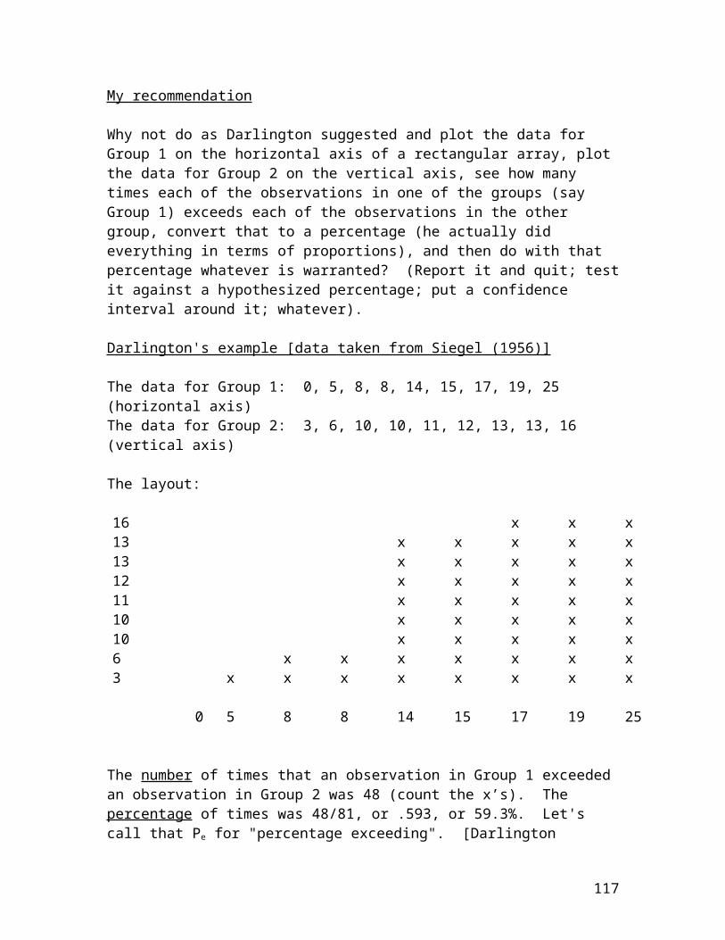
23
is a ratio-level variable. My advice: Try if at all posssible to avoid such situations, but if you are unable todo so consult your favorite statistician.
The bottom line(s)
If you are seriously interested in investigating the relationship between two variables, you should attend to thefollowing matters, in the order in which they are listed:
1. Phrase the research question in as clear and concise a manner as possible. Example: "What is the relationship between height and weight?" reads better than "What is the relationship between how tall you are and how much you weigh?"
2. Always start with design, then instrumentation, then analysis. For the height/weight research question, some sort of survey design is called for, with valid and reliablemeasurement of both variables, and employing one or more of the statistical analyses discussed above. A stratified random sampling design (stratifying on sex, because sex is amoderator of the relationship between height and weight), using an electronic stadiometer to measure height and an electronic balance beam scale to measure weight, and carrying out conventional linear regression analyses within sex would appear to be optimal.
3. Interpret the results accordingly.
References
Agresti, A. (1990). Categorical data analysis. New York: Wiley.
Campbell, D.T., & Kenny, D.A. (1999). A primer on regression artifacts. New York: Guilford.
24
Cohen, J. (1960). A coefficient of agreement for nominal scales. Educational and Psychological Measurement, 20, 37-46.
Cronbach, L.J. (1951). Coefficient alpha and the internal structure of tests. Psychometrika, 16, 297-334.
Diaconis, P., & Efron, B. (1983). Computer-intensive methods in statistics. Scientific American, 248 (5), 116-130.
Dretzke, B.J. (2001). Statistics with Microsoft Excel (2nd ed.). Saddle River, NJ: Prentice-Hall.
Edgington, E.S. (1995). Randomization tests (3rd. ed.). New York: Dekker.
Engstrom, J.L. (1988). Assessment of the reliability of physical measures. Research in Nursing & Health, 11, 383-389.
Fisher, R.A. (1958). Statistical methods for research workers (13th ed.). New York: Hafner.
Fleiss, J.L., Cohen, J., & Everitt, B.S. (1969). Large sample standard errors of kappa and weighted kappa. Psychological Bulletin, 72, 323-327.
Goodman, L. A. & Kruskal, W. H. (1979). Measures of association for cross classifications. New York: Springer-Verlag.
Knapp, T.R. (1977). The unit-of-analysis problem in applications of simple correlation analysis to educational research. Journal of Educational Statistics, 2, 171-196.
25
Knapp, T.R. (1979). Using incidence sampling to estimate covariances. Journal
of Educational Statistics, 4, 41-58.
Knapp, T.R. (1999). The analysis of the data for two-way contingency tables. Research in Nursing & Health, 22, 263-268. Knapp, T.R., Noblitt, G.L., & Viragoontavan, S. (2000). Traditional vs. "resampling" approaches to statistical inferences regarding correlation coefficients. Mid-Western Educational Researcher, 13 (2), 34-36.
Korn, E.L, & Graubard, B.I. (1998). Scatterplots with survey data. The American Statistician, 52 (1), 58-69.
Krippendorff, K. (1980). Content analysis: An introductionto its methodology. Thousand Oaks, CA: Sage.
Levin, J.R. (1993). Statistical significance testing from three perspectives. Journal of Experimental Education, 61, 378-382.
Macnaughton, D. (January 28, 2002). Definition of "Relationship Between Variables". Internet posting.
Muchinsky, P.M. (1996). The correction for attenuation. Educational and Psychological Measurement, 56, 63-75.
Osborne, J. W. (2000). Advantages of hierarchical linear modeling. Practical Assessment, Research, & Evaluation , 7 (1). Available online.
Raju, N.S., & Brand, P.A. (2003). Determining the significance of correlations corrected for unreliability andrange restriction. Applied Psychological Measurement, 27 (1), 52-71.
26
Raudenbush, S. W., & Bryk, A.S. (2002). Hierarchical linear models: Applications and data analysis methods . (2nd.ed.) Newbury Park, CA: Sage.
Robinson, W.S. (1950). Ecological correlations and the behavior of individuals. American Sociological Review, 15, 351-357.
Robinson, W.S. (1957). The statistical measurement of agreement. American Sociological Review, 22, 17-25.
Rodgers, J.L., & Nicewander, W.A. (1988). Thirteen ways tolook at the correlation coefficient. The American Statistician, 42 (1), 59-66.
Shaver, J.P. (1993). What statistical significance is, andwhat it is not. Journal of Experimental Education, 61, 293-316.
Simon, G.A. (1978). Efficacies of measures of association for ordinal contingency tables. Journal of the American Statistical Association, 73 (363), 545-551.
Sirotnik, K.A., & Wellington, R. (1974). Incidence sampling: An integrated theory for "matrix sampling". Journal of Educational Measurement, 14, 343-399.
Somers, R.H. (1962). A new asymmetric measure of association for ordinal variables. American Sociological Review, 27, 799-811.
Stanley, J.C. (1964). Measurement in today's schools (4th ed.). New York: Prentice-Hall.
Wilkinson, L. (2001). Presentation graphics. In N.J. Smelser & P.B. Baltes (Eds.), International encyclopedia of the social and behavioral sciences. Amsterdam: Elsevier.
27
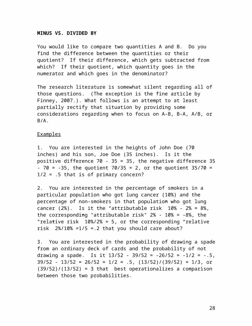
MINUS VS. DIVIDED BY
You would like to compare two quantities A and B. Do you find the difference between the quantities or their quotient? If their difference, which gets subtracted from which? If their quotient, which quantity goes in the numerator and which goes in the denominator?
The research literature is somewhat silent regarding all of those questions. (The exception is the fine article by Finney, 2007.). What follows is an attempt to at least partially rectify that situation by providing some considerations regarding when to focus on A-B, B-A, A/B, or B/A.
Examples
1. You are interested in the heights of John Doe (70 inches) and his son, Joe Doe (35 inches). Is it the positive difference 70 - 35 = 35, the negative difference 35- 70 = -35, the quotient 70/35 = 2, or the quotient 35/70 = 1/2 = .5 that is of primary concern?
2. You are interested in the percentage of smokers in a particular population who got lung cancer (10%) and the percentage of non-smokers in that population who got lung cancer (2%). Is it the “attributable risk” 10% - 2% = 8%, the corresponding "attributable risk" 2% - 10% = -8%, the “relative risk” 10%/2% = 5, or the corresponding “relative risk” 2%/10% =1/5 =.2 that you should care about?
3. You are interested in the probability of drawing a spadefrom an ordinary deck of cards and the probability of not drawing a spade. Is it 13/52 - 39/52 = -26/52 = -1/2 = -.5,39/52 - 13/52 = 26/52 = 1/2 = .5, (13/52)/(39/52) = 1/3, or (39/52)/(13/52) = 3 that best operationalizes a comparison between those two probabilities.
28
4. You are interested in the change from pretest to posttest of an experimental group that had a mean of 20 on the pretest and a mean of 30 on the posttest, as opposed to a control group that had a mean of 20 on the pretest and a mean of 10 on the posttest. Which numbers should you compare, and how should you compare them?
Considerations for those examples
1. The negative difference isn't very useful, other than asan indication of how much "catching up" Joe needs to do. Asfar as the other three alternatives are concerned, it all depends upon what you want to say after you make the comparison. Do you want to say something like "John is 35 inches taller than Joe"? "John is twice as tall as Joe"? "Joe is half as tall as John"?2. Again, the negative attributable risk is not very useful. The positive attributable risk is most natural ("Isthere a difference in the prevalence of lung cancer between smokers and non-smokers?"). The relative risk (or an approximation to the relative risk called an "odds ratio") is the overwhelming choice of epidemiologists. They also favor the reporting of relative risks that are greater than 1 ("Smokers are five times as likely to get lung cancer") rather than those that are less than 1 ("Non-smokers are one-fifth as likely to get lung cancer"). One difficulty with relative risks is that if the quantity that goes in thedenominator is zero you have a serious problem, since you can't divide by zero. (A common but unsatisfactory solutionto that problem is to call such a quotient "infinity".) Another difficulty with relative risks is that no distinction is made between a relative risk for small risks such as 2% and 1%, and for large risks such as 60% and 30%.
3. Both of the difference comparisons would be inappropriate, since it is a bit strange to subtract two things that are actually the complements of one another (theprobability of something plus the probability of not-that-something is always equal to 1). So it comes down to
29
whether you want to talk about the "odds in favor of" getting a spade ("1 to 3") or the "odds against" getting a spade ("3 to 1"). The latter is much more natural.
4. This very common comparison can get complicated. You probably don't want to calculate the pretest-to-posttest quotient or the posttest-to-pretest quotient for each of thetwo groups, for two reasons: (1) as indicated above, one or more of those averages might be equal to zero (because of how the "test" is scored); and (2) the scores often do not arise from a ratio scale. That leaves differences. But what differences? It would seem best to subtract the mean pretest score from the mean posttest score for each group (30 - 20 = 10 for the experimental group and 10 - 20 = -10 for the control group) and then to subtract those two differences from one another (10 -[-10] = 20, i.e., a "swing'"of 20 points), and that is what is usually done.
What some of the literature has to say
I mentioned above that the research literature is "somewhat silent" regarding the choice between differences and quotients. But there are a few very good sources, in addition to Finney (2007), regarding the advantages and disadvantages of each.
The earliest reference I could find is an article in Volume 1, Number 1 of the Peabody Journal of Education by Sherrod (1923). In that article he summarized a number of quotientsthat had just been developed, including the familiar mental age divided by chronological age, and made a couple of briefcomments regarding differences, but did not provide any arguments concerning preferences for one vs. the other. One of the best pieces (in my opinion) is an article that appeared recently on the American College of Physicians' website. The author pointed out that although differences and quotients of percentages are calculated from the same data, differences often "feel" smaller than quotients.
30
Another relevant source is the article that H.P. Tam and I wrote a few years ago (Knapp & Tam, 1997) concerning proportions, differences between proportions, and quotients of proportions. (A proportion is just like a percentage, with the decimal point moved two places to the left.)
There are also a few good substantive studies in which choices were made, and the investigators defended such choices. For example, Kruger and Nesse (2004) preferred the male-to-female mortality ratio (quotient) to the difference between male and female mortality numbers. That ratio is methodologically similar to sex ratio at birth. Itis reasonably well known that male births are more common than female births in just about all cultures. (In the United States the sex ratio at birth is about 1.05, i.e., there are approximately five percent more male births than female births, on the average.)
The Global Youth Tobacco Survey Collaborating Group (2003) also chose the male-to-female ratio for comparing the tobacco use of boys and girls in the 13-15 years of age range.
In an interesting "twist", Baron, Neiderhiser, and Gandy (1997) asked samples of Blacks and samples of Whites to estimate what the Black-to-White ratio was for deaths from various causes, and compared those estimates to the actual ratios as provided by the Centers for Disease Control (CDC).
Some general considerations
It all depends upon what the two quantities to be compared are.
1. Let's first consider situations such as that of Example #1 above, where we want to compare a single measurement on avariable with another single measurement on that variable. In that case, the reliability and validity with which the
31
variable can be measured are crucial. You should compare the errors for the difference between two measurements with the errors for the quotient of two measurements. The relevant chapters in the college freshman physics laboratorymanual (of all places) written by Simanek (2005) is especially good for a discussion of such errors. It turns out that the error associated with a difference A-B is the sum of the errors for A and B, whereas the error associated with a quotient A/B is the difference between the relative errors for A and for B. (The relative error for A is the error in A divided by A, and the relative error for B is theerror for B divided by B.)
2. The most common comparison is for two percentages. If the two percentages are independent, i.e., they are not for the same observations or matched pairs of observations, the difference between the two is usually to be preferred; but if the percentages are based upon huge numbers of observations in epidemiological investigations the quotient of the two is the better choice, and usually with the largerpercentage in the numerator and the smaller percentage in the denominator.
If the percentages are not independent, e.g., the percentageof people who hold a particular attitude at Time 1 compared to the percentage of those same people who hold that attitude at Time 2, the difference (usually the Time 2 percentage minus the Time 1 percentage, i.e., the change, even if that is negative) is almost always to be preferred. Quotients of non-independent percentages are very difficult to handle statistically.
3. Quotients of probabilities are usually preferred to their differences.
4. On the other hand, comparisons of means that are not percentages (did you know that percentages are special kindsof means, with the only possible "scores" 0 and 100?) rarelyinvolve quotients. As I pointed out in Example #4 above,
32
there are several differences that might be of interest. For randomized experiments for which there is no pretest, subtracting the mean posttest score for the control group from the mean posttest score for the experimental group is most natural and most conventional. For pretest/posttest designs the "difference between the differences" or the difference between "adjusted" posttest means (via the analysis of covariance, for example) is the comparison of choice.
5. There are all sorts of change measures to be found in the literature, e.g., the difference between the mean score at Time 2 and the mean score at Time 1 divided by the mean score at Time 1 (which would provide an indication of the percent "improvement"). Many of those measures have sparkeda considerable amount of controversy in the methodological literature, and the choice between expressing change as a difference or as a quotient is largely idiosyncratic.
The absolute value of differences
It is fairly common for people to concentrate on the absolute value of a difference, in addition to, or instead of, the "raw" difference. The absolute value of the difference between A and B, usually denoted as |A-B|, which is the same as |B-A|, is especially relevant when the discrepancy between the two is of interest, irrespective of which is greater.
Statistical inference
The foregoing discussion assumed that the data in hand are for a full population (even if the "N" is very small). If the data are for a random sample of a population, the preference between a difference statistic and a quotient statistic often depends upon the existence and/or complexityof the sampling distributions for such statistics. For example, the sampling distribution for a difference between two independent percentages is well known and
33
straightforward (either the normal distribution or the chi-square distribution can be used) whereas the sampling distribution for the odds ratio is a real mess.
A controversial example
It is very common during a presidential election campaign tohear on TV something like this: “In the most recent opinionpoll, Smith is leading Jones by seven points.” What is meant by a “point”? Is that information important? If so, can the difference be tested for statistical significance and/or can a confidence interval be constructed around it?
The answer to the first question is easy. A “point” is a percentage. For example, 46% of those polled might have favored Smith and 39% might have favored Jones, a differenceof seven “points” or seven percent. Since those two numbersdon’t add to 100, there might be other candidates in the race, some of those polled had no preferences, or both. [I’ve never heard anybody refer to the ratio of the 46 to the 39. Have you?]
It is the second question that has sparked considerable controversy. Some people (like me) don’t think the difference is important; what matters is the actual % support for each of the candidates. (Furthermore, the two percentages are not independent, since their sum plus the sum of the percentages for other candidates plus the percentage of people who expressed no preferences must add to 100.) Other people (like my friend Milo Schield) think itis very important, not only for opinion polls but also for things like the difference between the percentage of people in a sample who have blue eyes and the percentage of people in that same sample who have green eyes (see Simon, 2004), and other contexts.
Alas (for me), differences between percentages calculated onthe same scale for the same sample can be tested for statistical significance and confidence intervals for such
34
differences can be determined. See Kish (1965) and Scott and Seber (1983).
Financial example: "The Rule of 72"
[I would like to thank my former colleague and good friend at The Ohio State University, Dick Shumway, for referring meto this rule that his father, a banker, first brought to hisattention.]
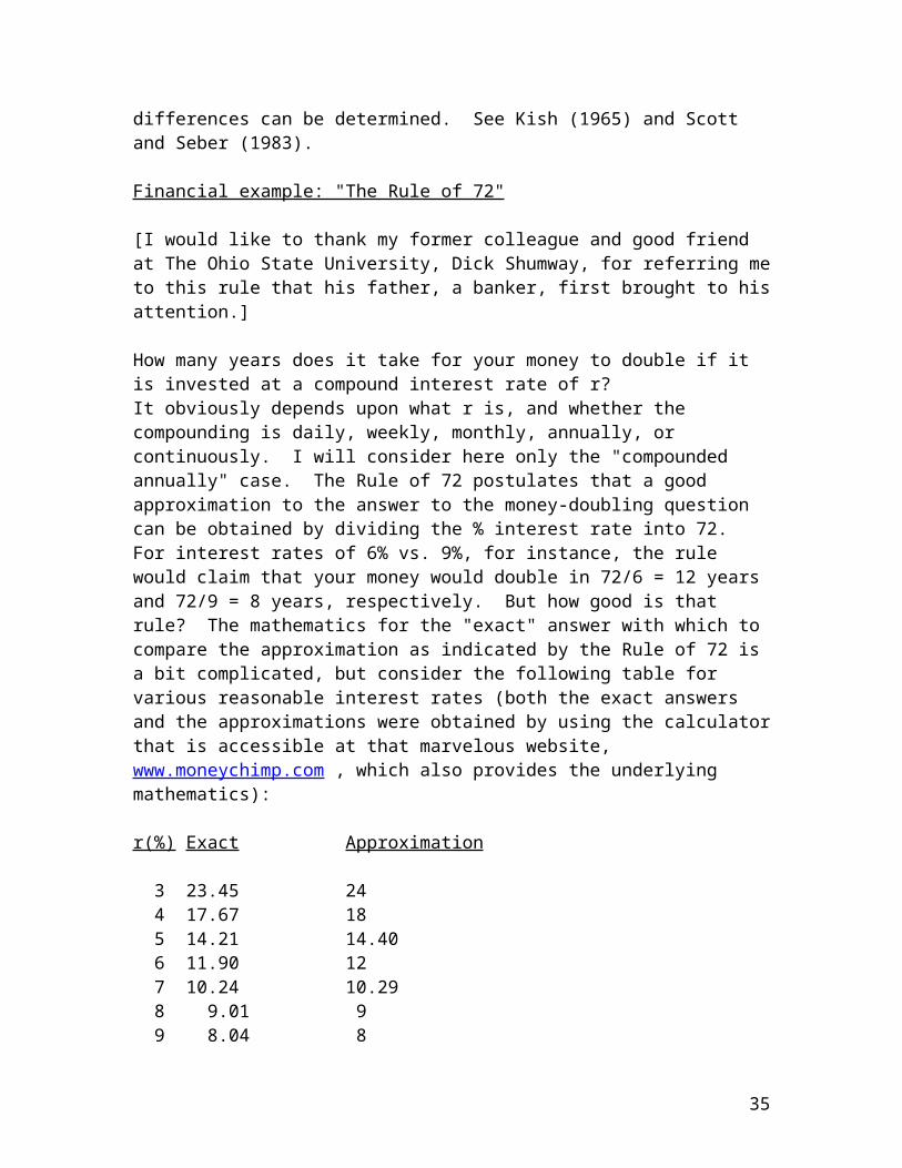
How many years does it take for your money to double if it is invested at a compound interest rate of r?It obviously depends upon what r is, and whether the compounding is daily, weekly, monthly, annually, or continuously. I will consider here only the "compounded annually" case. The Rule of 72 postulates that a good approximation to the answer to the money-doubling question can be obtained by dividing the % interest rate into 72. For interest rates of 6% vs. 9%, for instance, the rule would claim that your money would double in 72/6 = 12 years and 72/9 = 8 years, respectively. But how good is that rule? The mathematics for the "exact" answer with which to compare the approximation as indicated by the Rule of 72 is a bit complicated, but consider the following table for various reasonable interest rates (both the exact answers and the approximations were obtained by using the calculatorthat is accessible at that marvelous website, www.moneychimp.com , which also provides the underlying mathematics):
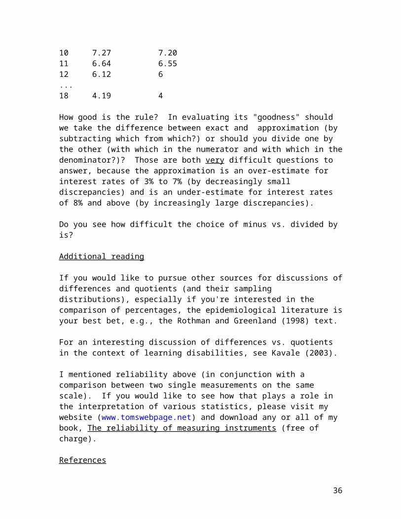
How good is the rule? In evaluating its "goodness" should we take the difference between exact and approximation (by subtracting which from which?) or should you divide one by the other (with which in the numerator and with which in thedenominator?)? Those are both very difficult questions to answer, because the approximation is an over-estimate for interest rates of 3% to 7% (by decreasingly small discrepancies) and is an under-estimate for interest rates of 8% and above (by increasingly large discrepancies).
Do you see how difficult the choice of minus vs. divided by is?
Additional reading
If you would like to pursue other sources for discussions ofdifferences and quotients (and their sampling distributions), especially if you're interested in the comparison of percentages, the epidemiological literature isyour best bet, e.g., the Rothman and Greenland (1998) text.
For an interesting discussion of differences vs. quotients in the context of learning disabilities, see Kavale (2003).
I mentioned reliability above (in conjunction with a comparison between two single measurements on the same scale). If you would like to see how that plays a role in the interpretation of various statistics, please visit my website (www.tomswebpage.net) and download any or all of my book, The reliability of measuring instruments (free of charge).
References
36
Baron, J., Neiderhiser, B., & Gandy, O.H., Jr. (1997). Perceptions and attributions of race differences in health risks. (On Jonathan Baron's website.)
Finney, D.J. (2007). On comparing two numbers. Teaching Statistics, 29 (1), 17-20.
Global Youth Tobacco Survey Collaborating Group. (2003). Differences in worldwide tobacco use by gender: Findings from the Global Youth Tobacco Survey. Journal of School Health, 73 (6), 207-215.
Kavale, K. (2003). Discrepancy models in the identification of learning disability. Paper presented at the Learning Disabilities Summit organized by the Departmentof Education in Washington, DC.
Kish, L. (1965). Survey sampling. New York: Wiley.
Knapp, T.R., & Tam, H.P. (1997). Some cautions concerning inferences about proportions, differences between
proportions, andquotients of proportions. Mid-Western Educational
Researcher, 10 (4),11-13.
Kruger, D.J., & Nesse, R.M. (2004). Sexual selection and the male:female mortality ratio. Evolutionary Psychology, 2, 66-85.
Rothman, K.J., & Greenland, S. (1998). Modern epidemiology(2nd. ed.). Philadelphia: Lippincott, Williams, & Wilkins.
Scott, A.J., & Seber, G.A.F. (1983). Difference of proportions from the same survey. The American Statistician, 37 (4), Part 1, 319-320.
37
Sherrod, C.C. (1923). The development of the idea of quotients in education. Peabody Journal of Education, 1 (1), 44-49.
Simanek, D. (2005). A laboratory manual for introductory physics. Retrievable in its entirety from: http://www.lhup.edu/~dsimanek/scenario/contents.htm
Simon, S. (November 9, 2004). Testing multinomial proportions. StATS Website.
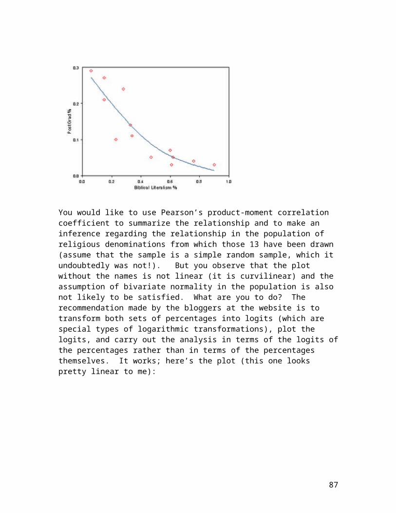
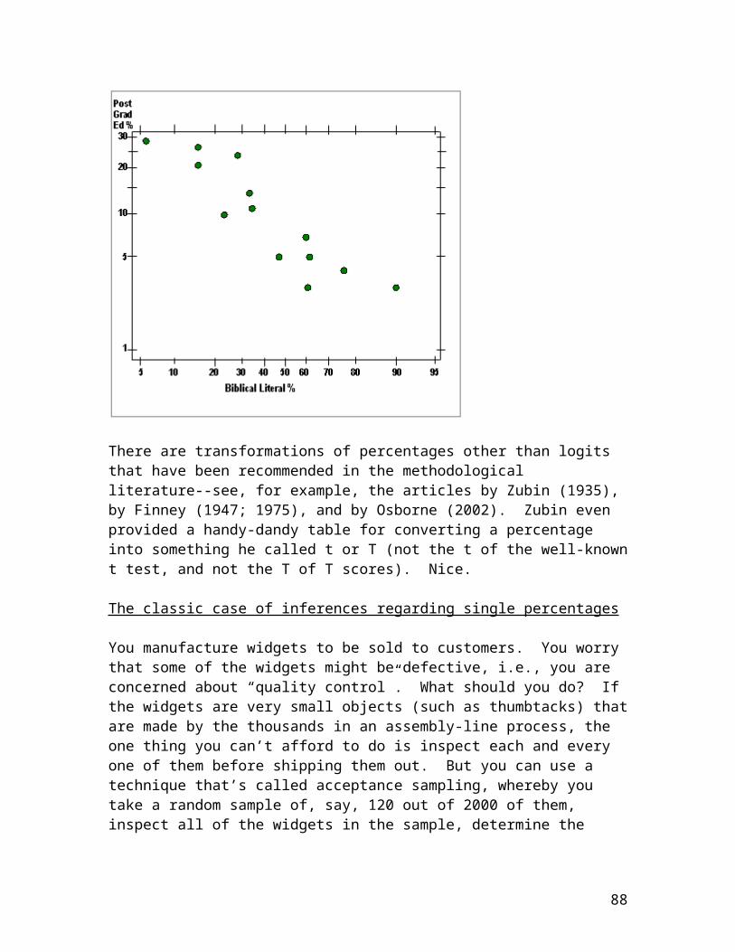
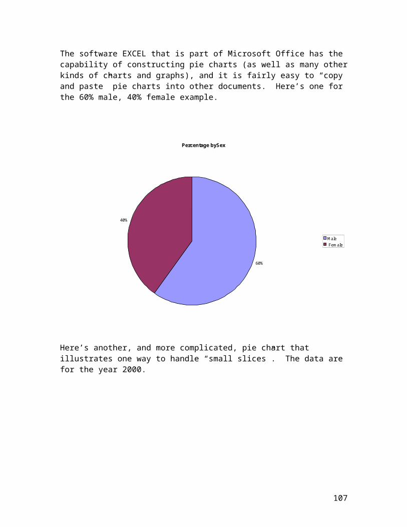
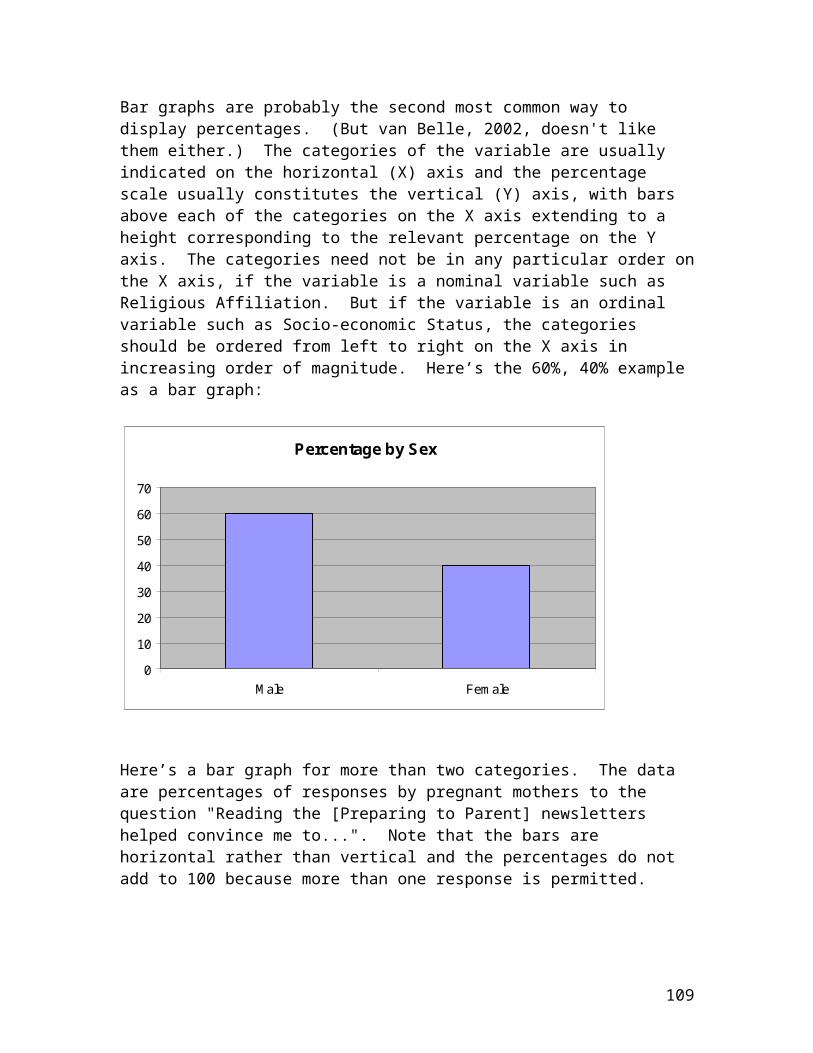
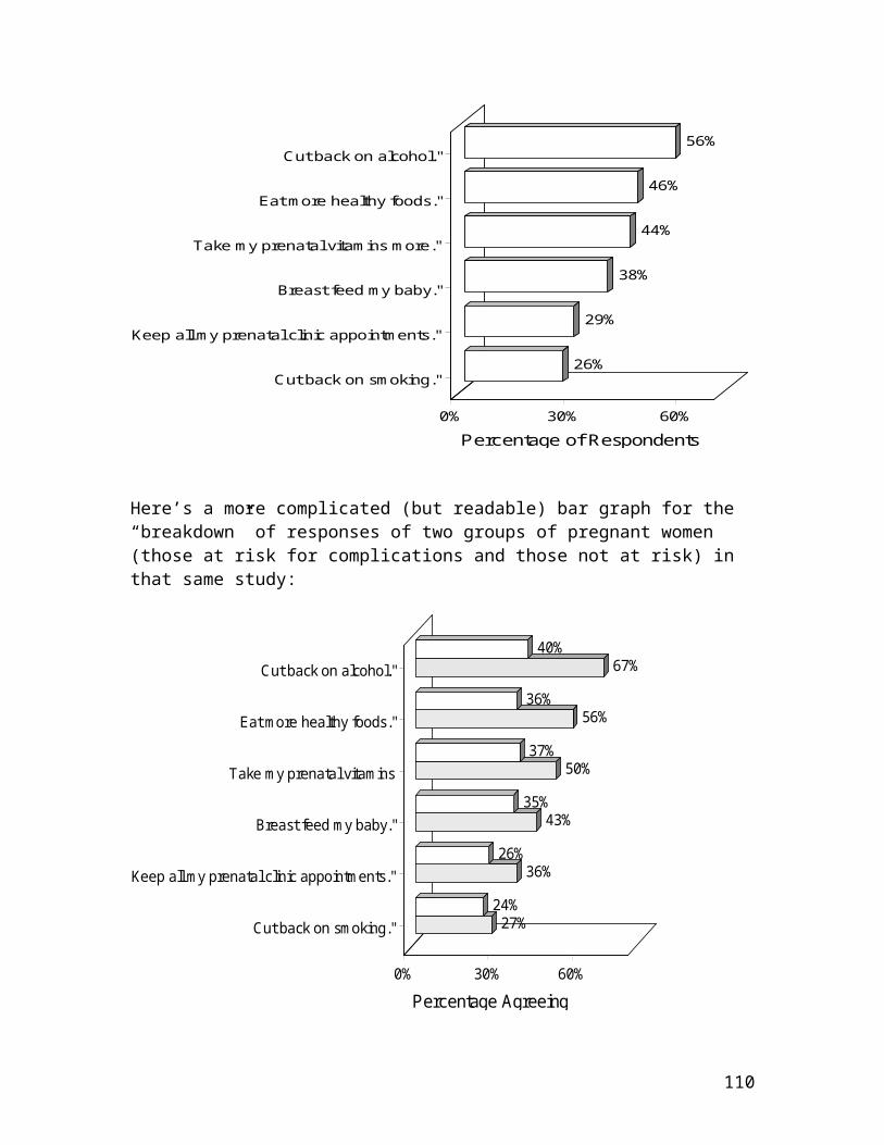
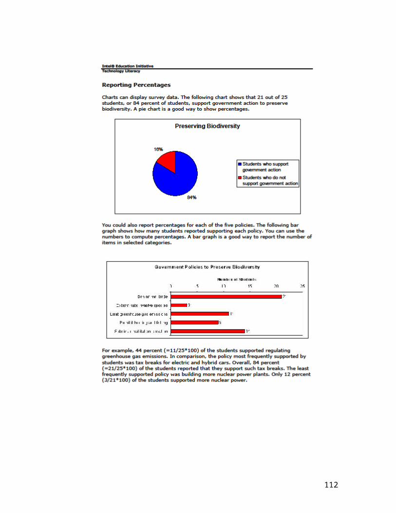
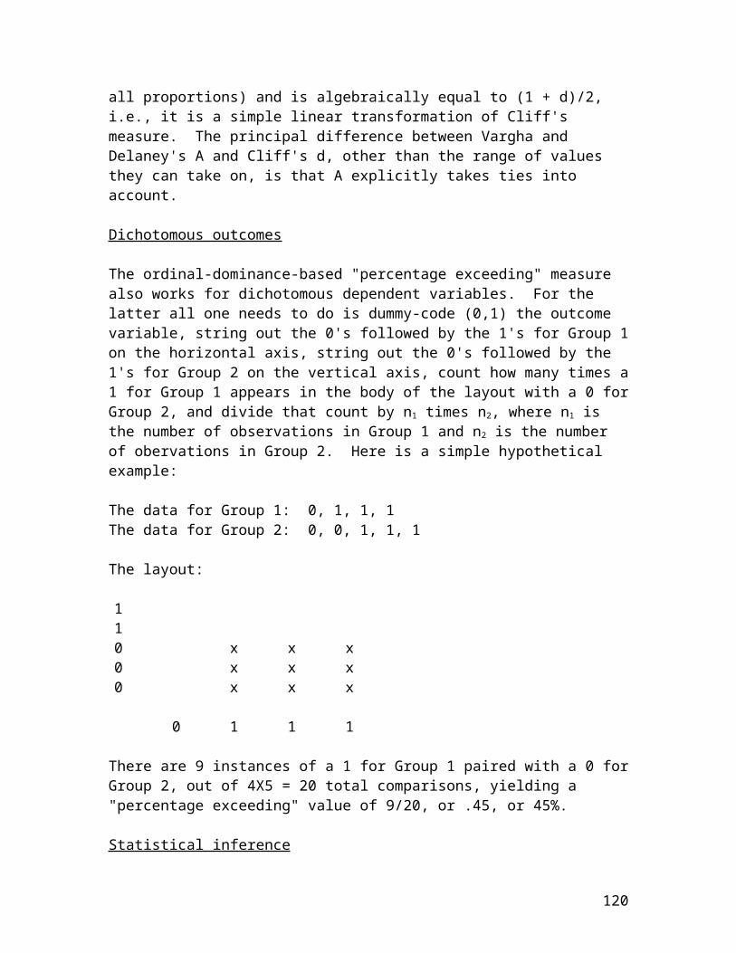
PERCENTAGES: THE MOST USEFUL STATISTICS EVER INVENTED
"Eighty percent of success is showing up."- Woody Allen
“Baseball is ninety percent mental and the other half is physical.”- Yogi Berra
"Genius is one percent inspiration and ninety-nine percent perspiration."- Thomas Edison
39
Preface You know what a percentage is. 2 out of 4 is 50%. 3 is 25%of 12. Etc. But do you know enough about percentages? Is a percentage the same thing as a fraction or a proportion? Should we take the difference between two percentages or their ratio? If their ratio, which percentage goes in the numerator and which goes in the denominator? Does it matter? What do we mean by something being statistically significant at the 5% level? What is a 95% confidence interval? Those questions, and much more, are what this monograph is all about.
In his fine article regarding nominal and ordinal bivariate statistics, Buchanan (1974) provided several criteria for a good statistic, and concluded: “The percentage is the most useful statistic ever invented…” (p. 629). I agree, and thus my choice for the title of this work. In the ten chapters that follow, I hope to convince you of the defensibility of that claim.
The first chapter is on basic concepts (what a percentage is, how it differs from a fraction and a proportion, what sorts of percentage calculations are useful in statistics, etc.) If you’re pretty sure you already understand such things, you might want to skip that chapter (but be preparedto return to it if you get stuck later on!).
In the second chapter I talk about the interpretation of percentages, differences between percentages, and ratios of percentages, including some common mis-interpretations and pitfalls in the use of percentages.
Chapter 3 is devoted to probability and its explanation in terms of percentages. I also include in that chapter a discussion of the concept of “odds” (both in favor of, and against, something). Probability and odds, though related, are not the same thing (but you wouldn’t know that from reading much of the scientific and lay literature).
40
Chapter 4 is concerned with a percentage in a sample vis-à-vis the percentage in the population from which the sample has been drawn. In my opinion, that is the most elementary notion in inferential statistics, as well as the most important. Point estimation, interval estimation (confidence intervals), and hypothesis testing (significancetesting) are all considered.
The following chapter goes one step further by discussing inferential statistical procedures for examining the difference between two percentages and the ratio of two percentages, with special attention to applications in epidemiology.
The next four chapters are devoted to special topics involving percentages. Chapter 6 treats graphical procedures for displaying and interpreting percentages. It is followed by a chapter that deals with the use of percentages to determine the extent to which two frequency distributions overlap. Chapter 8 discusses the pros and cons of dichotomizing a continuous variable and using percentages with the resulting dichotomy. Applications to the reliability of measuring instruments (my second most favorite statistical concept--see Knapp, 2009) are explored in Chapter 9. The final chapter attempts to summarize things and tie up loose ends.
There is an extensive list of references, all of which are cited in the text proper. You may regard some of them as “old” (they actually range from 1919 to 2009). I like oldreferences, especially those that are classics and/or are particularly apt for clarifying certain points. [And I’m old too.]
41
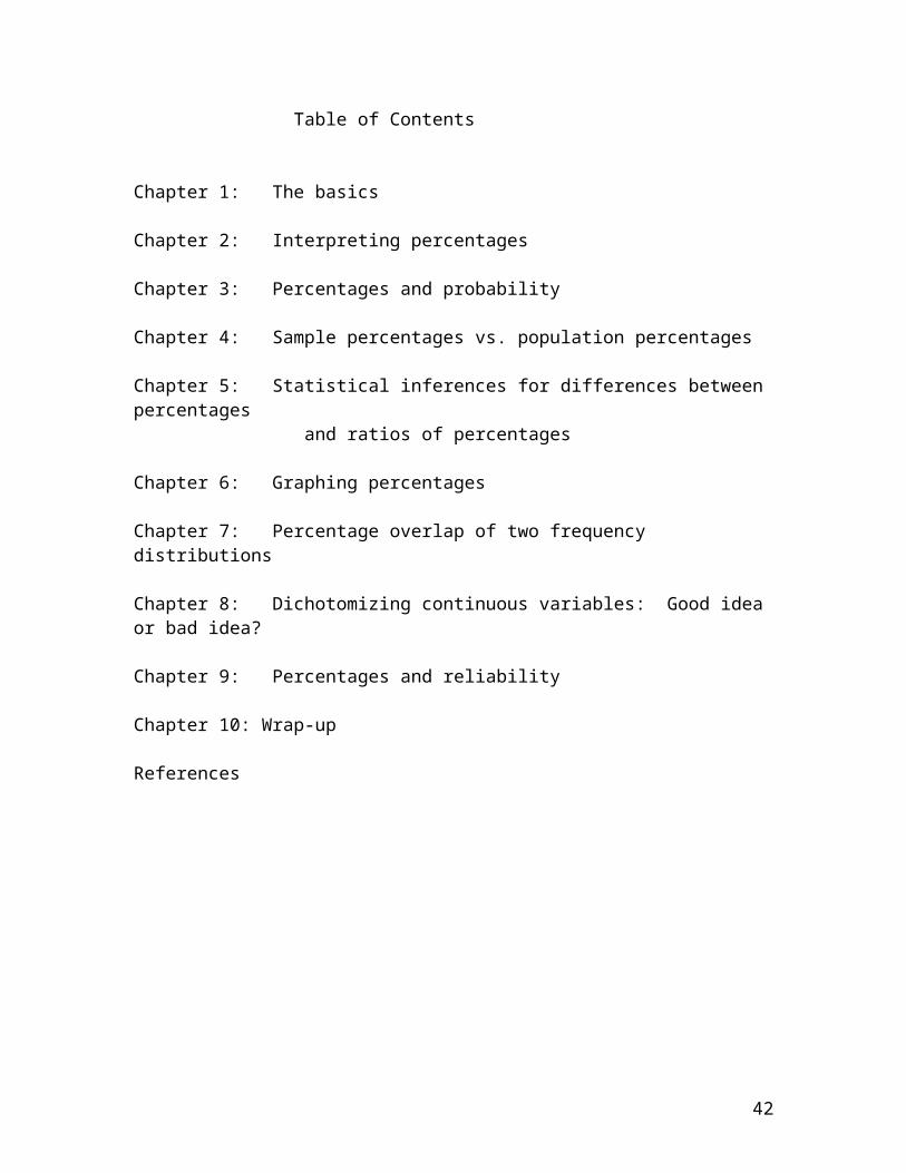
Table of Contents
Chapter 1: The basics
Chapter 2: Interpreting percentages
Chapter 3: Percentages and probability
Chapter 4: Sample percentages vs. population percentages
Chapter 5: Statistical inferences for differences between percentages
and ratios of percentages
Chapter 6: Graphing percentages
Chapter 7: Percentage overlap of two frequency distributions
Chapter 8: Dichotomizing continuous variables: Good idea or bad idea?
Chapter 9: Percentages and reliability
Chapter 10: Wrap-up
References
42
Chapter 1: The basics
What is a percentage?
A percentage is a part of a whole. It can take on values between 0 (none of the whole) and 100 (all of the whole). The whole is called the base. The base must ALWAYS be reported whenever a percentage is determined.
Example: There are 20 students in a classroom, 12 of whom are males and 8 of whom are females. The percentage of males is 12 “out of” 20, or 60%. The percentage of females is 8 “out of” 20, or 40%. (20 is the base.)
To how many decimal places should a percentage be reported?
One place to the right of the decimal point is usually sufficient, and you should almost never report more than two. For example, 2 out of 3 is 66 2/3 %, which rounds to 66.67% or 66.7%. [To refresh your memory, you round down ifthe fractional part of a mixed number is less than 1/2 or ifthe next digit is 0, 1, 2, 3, or 4; you round up if the fractional part is greater than or equal to 1/2 or if the next digit is 5, 6, 7, 8, or 9.] Computer programs can report numbers to ten or more decimal places, but that doesn’t mean that you have to. I believe that people who report percentages to several decimal places are trying to impress the reader (consciously or unconsciously).
Lang and Secic (2006) provide the following rather rigid rule:
“When the sample size is greater than 100, report percentages to no more than one decimal place. When sample size is less than 100, report percentages in wholenumbers. When sample size is less than, say, 20,
consider reporting the actual numbers rather than percentages.” (p. 5)
43
[Their rule is just as appropriate for full populations as it is for samples. And they don’t say it, perhaps because it is obvious, but if the size of the group is equal to 100,be it sample or population, the percentages are the same as the numerators themselves, with a % sign tacked on.]
How does a percentage differ from a fraction and a proportion?
Fractions and proportions are also parts of wholes, but bothtake on values between 0 (none of the whole) and 1 (all of the whole), rather than between 0 and 100. To convert from a fraction or a proportion to a percentage you multiply by 100 and add a % sign. To convert from a percentage to a proportion you delete the % sign and divide by 100. That can in turn be converted to a fraction. For example, 1/4 multiplied by 100 is 25%. .25 multiplied by 100 is also 25%. 25% divided by 100 is .25, which can be expressed as afraction in a variety of ways, such as 25/100 or, in “lowestterms”, 1/4. (See the excellent On-Line Math Learning Center website for examples of how to convert from any of these part/whole statistics to any of the others.) But, surprisingly (to me, anyhow), people tend to react differently to statements given in percentage terms vs. fractional terms, even when the statements are mathematically equivalent. (See the October 29, 2007 post by Roger Dooley on the Neuromarketing website. Fascinating.)
Most authors of statistics books, and most researchers, prefer to work with proportions. I prefer percentages [obviously, or I wouldn’t have written this monograph!], as does my friend Milo Schield, Professor of Business Administration and Director of the W. M. Keck Statistical Literacy Project at Augsburg College in Minneapolis, Minnesota. (See, for example, Schield, 2008). One of the reasons I don't like to talk about proportions is that they have another meaning in mathematics in general: "a is in the
44
same proportion to b as c is to d". People studying statistics could easily be confused about those two different meanings of the term "proportion". One well-known author (Gerd Gigerenzer) prefers fractions toboth percentages and proportions. In his book (Gigerenzer, 2002) and in a subsequent article he co-authored with several colleagues (Gigerenzer, et al., 2007), he advocates an approach that he calls the method of “natural frequencies” for dealing with percentages. For example, instead of saying something like “10% of smokers get lung cancer”, he would say “100 out of every 1000 smokers get lung cancer” [He actually uses breast cancer to illustrate his method]. Heynen (2009) agrees. But more about that inChapter 3, in conjunction with positive diagnoses of diseases.
Is there any difference between a percentage and a percent?
The two terms are often used interchangeably (as I do in this monograph), but “percentage” is sometimes regarded as the more general term and “percent” as the more specific term. The AMA Manual of Style, the BioMedical Editor website, the Grammar Girl website, and Milo Schield have more to say regarding that distinction. The Grammar Girl (Mignon Fogarty) also explains whether percentage takes a singular or plural verb, whether to use words or numbers before the % sign, whether to have a leading 0 before a decimal number that can’t be greater than 1, and all sorts of other interesting things.
Do percentages have to add to 100?
A resounding YES, if the percentages are all taken on the same base for the same variable, if only one “response” is permitted, and if there are no missing data. For a group ofpeople consisting of both males and females, the % male plusthe % female must be equal to 100, as indicated in the aboveexample (60+40=100). If the variable consists of more than
45
two categories (a two-categoried variable is called a dichotomy), the total might not add to 100 because of rounding. As a hypothetical example, consider what might happen if the variable is something like Religious Affiliation and you have percentages reported to the nearesttenth for a group of 153 people of 17 different religions. If those percentages add exactly to 100 I would be terribly surprised.
Several years ago, Mosteller, Youtz, and Zahn (1967) determined that the probability (see Chapter 3) of rounded percentages adding exactly to 100 is perfect for two categories, approximately 3/4 for three categories, approximately 2/3 for four categories, and approximately √6/cπ for c ≥5, where c is the number of categories and π isthe well-known ratio of the circumference of a circle to itsdiameter (= approximately 3.14). Amazing!
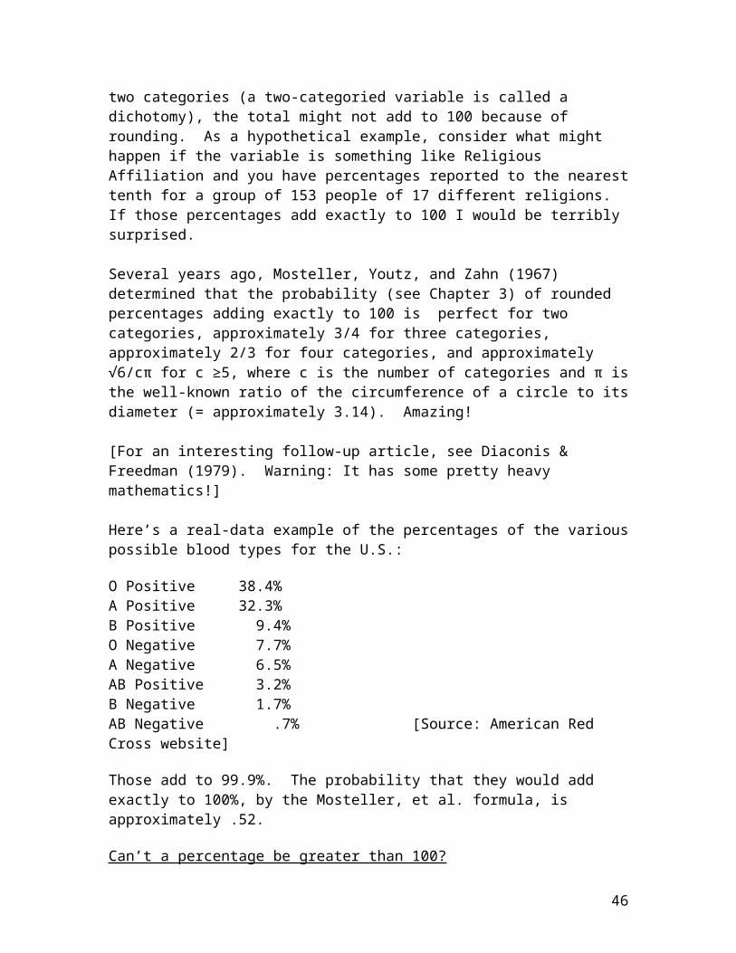
[For an interesting follow-up article, see Diaconis & Freedman (1979). Warning: It has some pretty heavy mathematics!] Here’s a real-data example of the percentages of the variouspossible blood types for the U.S.:
O Positive 38.4% A Positive 32.3% B Positive 9.4% O Negative 7.7% A Negative 6.5% AB Positive 3.2% B Negative 1.7% AB Negative .7% [Source: American Red Cross website]
Those add to 99.9%. The probability that they would add exactly to 100%, by the Mosteller, et al. formula, is approximately .52.
Can’t a percentage be greater than 100?
46
I said above that percentages can only take on values between 0 and 100. There is nothing less than none of a whole, and there is nothing greater than all of a whole. But occasionally [too often, in my opinion, but Milo Schielddisagrees with me] you will see a statistic such as “Her salary went up by 200%” or “John is 300% taller than Mary”. Those examples refer to a comparison in terms of a percentage, not an actual percentage. I will have a great deal to say about such comparisons in the next chapter and in Chapter 5.
Why are percentages ubiquitous?
People in general, and researchers in particular, have always been interested in the % of things that are of a particular type, and they always will be. What % of voters voted for Barack Obama in the most recent presidential election? What % of smokers get lung cancer? What % of thequestions on a test do I have to answer correctly in order to pass?
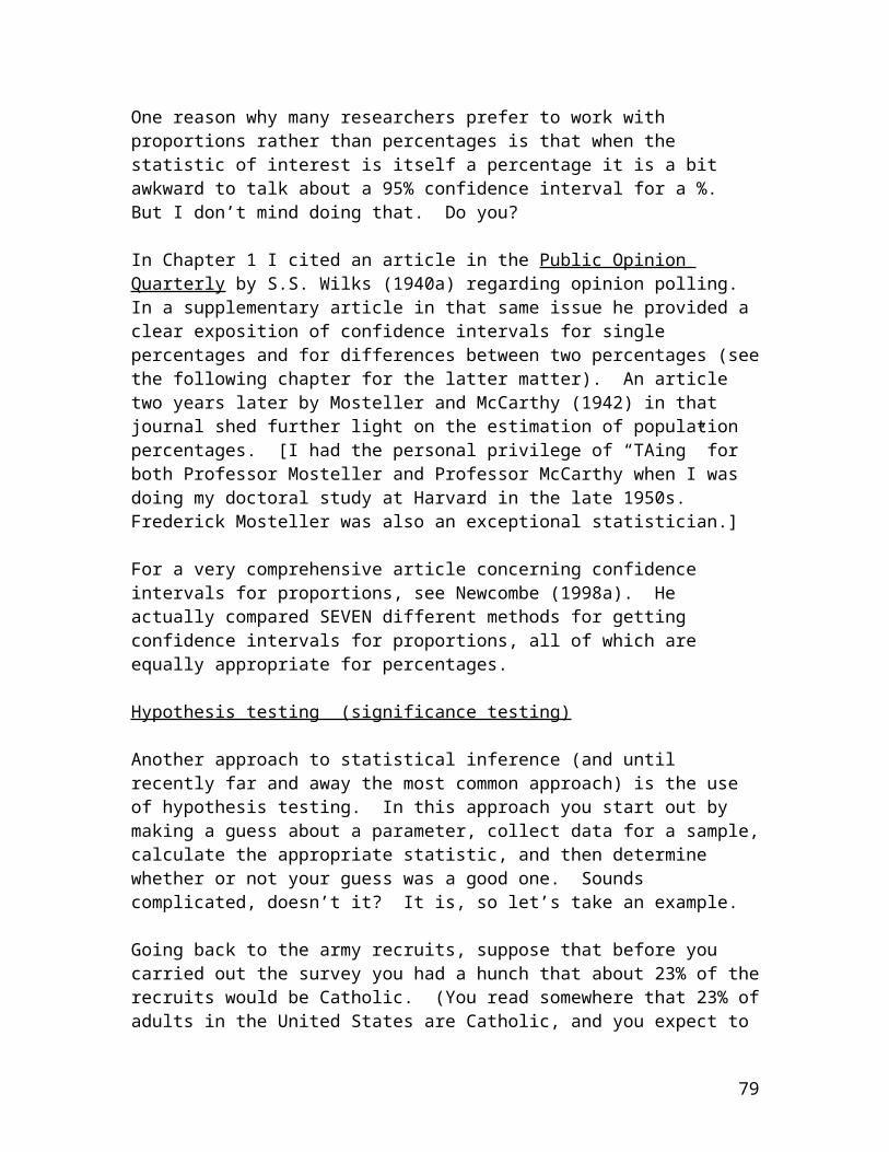
An exceptionally readable source about opinion polling is the article in the Public Opinion Quarterly by Wilks (1940a), which was written just before the entrance of the U.S. into World War II, a time when opinions regarding that war were diverse and passionate. I highly recommend that article to those of you who want to know how opinion polls SHOULD work. S.S. Wilks was an exceptional statistician.
What is a rate?
A rate is a special kind of percentage, and is most often referred to in economics, demography, and epidemiology. An interest rate of 10%, for example, means that for every dollar there is a corresponding $1.10 that needs to be takeninto consideration (whether it is to your advantage or to your disadvantage).
47
There is something called “The Rule of 72” regarding interest rates. If you want to determine how many years it would take for your money to double if it were invested at aparticular interest rate, compounded annually, divide the interest rate into 72 and you’ll have a close approximation.To take a somewhat optimistic example, if the rate is 18% itwould take four years (72 divided by 18 is 4) to double yourmoney. [You would actually have “only” 1.93877 times as much after four years, but that’s close enough to 2 for government work! Those of you who already know something about compound interest might want to check that.]
Birth rates and death rates are of particular concern in theanalysis of population growth or decline. In order to avoidsmall numbers, they are usually reported “per thousand” rather than “per hundred” (which is what a simple percent is). For example, if in the year 2010 there were to be six million births in the United States “out of” a population of300 million, the (“crude”) birth rate would be 6/300, or 2%, or 20 per thousand. If there were three million deaths in that same year, the (also “crude”) death rate would be 3/300, or 1%, or 10 per thousand.
One of the most interesting rates is the “response rate” forsurveys. It is the percentage of people who agree to participate in a survey. For some surveys, especially thosethat deal with sensitive matters such as religious beliefs and sexual behavior, the response rate is discouragingly low(and often not even reported), so that the results must be taken with more than the usual grain of salt.
Some rates are phrased in even different terms, e.g., parts per 100,000 or parts per million (the latter often used to express the concentration of a particular pollutant).
48
What kinds of calculations can be made with percentages?
The most common kinds of calculations involve subtraction and division. If you have two percentages, e.g., the percentage of smokers who get lung cancer and the percentageof non-smokers who get lung cancer, you might want to subtract one from the other or you might want to divide one by the other. Which is it better to do? That matter has been debated for years. If 10% of smokers get lung cancer and 2% of non-smokers get lung cancer (the two percentages are actually lower than that for the U.S.), the difference is 8% and the ratio is 5-to-1 (or 1-to-5, if you invert thatratio). I will have much more to say about differences between percentages and ratios of percentages in subsequent chapters. (And see the brief, but excellent, discussion of differences vs. ratios of percentages at the American College of Physicians website.)
Percentages can also be added and multiplied, although such calculations are less common than the subtraction or division of percentages. I’ve already said that percentagesmust add to 100, whenever they’re taken on the same base forthe same variable. And sometimes we’re interested in “the percentage of a percentage”, in which case two percentages are multiplied. For example, if 10% of smokers get lung cancer and 60% of them (the smokers who get lung cancer) aremen, the percentage of smokers who get cancer and are male is 60% of 10%, or 6%. (By subtraction, the other 4% are female.)
You also have to be careful about averaging percentages. If10% of smokers get lung cancer and 2% of non-smokers get lung cancer, you can’t just “split the difference” between those two numbers to get the % of people in general who get lung cancer by adding them together and dividing by two (to obtain 6%). The number of non-smokers far exceeds the number of smokers (at least in 2009), so the percentages have to be weighted before averaging. Without knowing how many smokers and non-smokers there are, all you know is that
49
the average lung cancer % is somewhere between 2% and 10%, but closer to the 2%. [Do you follow that?]
What is inverse percentaging?
You’re reading the report of a study in which there is some missing data (see the following chapter), with one of the percentages based upon an n of 153 and another based upon ann of 147. [153 is one of my favorite numbers. Do you know why? I’ll tell you at the end of this monograph.] You are particularly interested in a variable for which the percentage is given as 69.8, but the author didn’t explicitly provide the n for that percentage (much less the numerator that got divided by that n). Can you find out what n is, without writing to the author?
The answer is a qualified yes, if you’re good at “inverse percentaging”. There are two ways of going about it. The first is by brute force. You take out your trusty calculator and try several combinations of numerators with denominators of 153 and 147 and see which, if any, of them yield 69.8% (rounded to the nearest tenth of a percent). OR, you can use a book of tables, e.g., the book by Stone (1958), and see what kinds of percentages you get for what kinds of n’s.
Stone’s book provides percentages for all parts from 1 to n of n’s from 1 to 399. You turn to the page for an n of 153 and find that 107 is 69.9% of 153. (That is the closest % to 69.8.) You then turn to the page for 147 and find that 102 is 69.4% of 147 and 103 is 70.1% of 147. What is your best guess for the n and for the numerator that you care about? Since the 69.9% for 107 out of 153 is very close tothe reported 69.8% (perhaps the author rounded incorrectly or it was a typo?), since the 69.4% for 102 out of 147 is not nearly as close, and the 70.1% is also not as close (andis an unlikely typo), your best guess is 107 out of 153. But you of course could be wrong.
50
What about the unit of analysis and the independence of observations?
In my opinion, more methodological mistakes are made regarding the unit of analysis and the independence of observations than in any other aspect of a research study. The unit of analysis is the entity (person, classroom, school,…whatever) upon which any percentage is taken. The observations are the numbers that are used in the calculation, and they must be independent of one another.
If, for example, you are determining the percentage male within a group of 20 people, and there are 12 males and 8 females in the group (as above), the percentage of male persons is 12/20 or 60%. But that calculation assumes that each person is counted only once, there are no twins in the group, etc. If the 20 persons are in two different classrooms, with one classroom containing all 12 of the males and the other classroom containing all 8 of the females, then the percentage of male classrooms is 1/2 or 50%, provided the two classrooms are independent They could be dependent if, to take an admittedly extreme case, there were 8 male/female twin-pairs who were deliberately assigned to different classrooms, with 4 other males joiningthe 8 males in the male classroom. [Gets tricky, doesn’t it?]
One of the first researchers to raise serious concerns aboutthe appropriate unit of analysis and the possibility of non-independent observations was Robinson (1950) in his investigation of the relationship between race and literacy.He found (among other things) that for a set of data in the 1930 U.S. Census the correlation between a White/Black dichotomy and a Literate/Illiterate dichotomy was only .203 with individual person as the unit of analysis (n = 97,272) but was .946 with major geographical region as the unit of analysis (n = 9), the latter being a so-called “ecological” correlation between % Black and % Illiterate. His article created all sorts of reactions from disbelief to demands for
51
re-analyses of data for which something other than the individual person was used as the unit of analysis. It (hisarticle) was recently reprinted in the International Journalof Epidemiology, along with several commentaries by Subramanian, et al. (2009a, 2009b), Oakes (2009), Firebaugh (2009), and Wakefield (2009). I have also written a piece about the same problem (Knapp, 1977a).
What is a percentile?
A percentile is a point on a scale below which some percentage of things fall. For example, “John scored at the75th percentile on the SAT” means that 75% of the takers scored lower than he did and 25% scored higher. We don’t even know, and often don’t care, what his actual score was on the test. The only sense in which a percentile refers toa part of a whole is as a part of all of the people, not a part of all of the items on the test.
52
Chapter 2: Interpreting percentages
Since a percentage is simple to calculate (much simpler than, say, a standard deviation, the formula for which has ten symbols!), you would think that it is also simple to interpret. Not so, as this chapter will now show.
Small base
It is fairly common to read a claim such as “66 2/3 % of doctors are sued for malpractice”. The information that theclaimant doesn’t provide is that only three doctors were included in the report and two of them were sued. In the first chapter I pointed out that the base upon which a percentage is determined must be provided. There is (or should be) little interest in a study of just three persons,unless those three persons are very special indeed.
There is an interesting article by Buescher (2008) that discusses some of the problems with using rates that have small numbers in the numerator, even if the base itself is large. And in his commentary concerning an article in the journal JACC Cardiovascular Imaging, Camici (2009) advises caution in the use of any ratios that refer to percentages.
Missing data
The bane of every researcher’s existence is the problem of missing data. You go to great lengths in designing a study,preparing the measuring instruments, etc., only to find out that some people, for whatever reason, don’t have a measurement on every variable. This situation is very common for a survey in which questions are posed regarding religious beliefs and/or sexual behavior. Some people don’tlike to be asked such questions, and they refuse to answer them. What is the researcher to do? Entire books have beenwritten about the problem of missing data (e.g., Little & Rubin, 2002). Consider what happens when there is a
53
question in a survey such as “Do you believe in God?”, the only two response categories are yes and no, and you get 30 yeses, 10 nos, and 10 “missing” responses in a sample of 50 people. Is the “%yes” 30 out of 50 (=60%) or 30 out of 40 (= 75%)? And Is the “%no” 10 out of 50 (=20%) or 10 out of 40 (=25%)? If it’s out of 50, the percentages (60 and 20) don’t add to 100. If it’s out of 40, the base is 40, not the actual sample size of 50 (that’s the better way to deal with the problem…“no response” becomes a third category).
Overlapping categories
Suppose you’re interested in the percentages of people who have various diseases. For a particular population the percentage having AIDS plus the percentage having lung cancer plus the percentage having hypertension might very well add to more than 100 because some people might suffer from more than one of those diseases. I used this example in my little book entitled Learning statistics through playing cards (Knapp, 1996, p. 24). The three categories (AIDS, lung cancer, and hypertension) could “overlap”. In the technical jargon of statistics, they are not “mutually exclusive”.
Percent change
Whenever there are missing data (see above) the base changes. But when you’re specifically interested in percentchange the base also does not stay the same, and strange things can happen. Consider the example in Darrell Huff’s delightful book, How to lie with statistics (1954), of a manwhose salary was $100 per week and who had to take a 50% paycut to $50 per week because of difficult economic times. [(100-50)/100 = .50 or 50%.] Times suddenly improved and the person was subsequently given a 50% raise. Was his salary back to the original $100? No. The base has shiftedfrom 100 to 50. $50 plus 50% of $50 is $75, not $100. [Theillustrations by Irving Geis in Huff’s book are hilarious!] There are several other examples in the research literature
54
and on the internet regarding the problem of % decrease followed by % increase, as well as % increase followed by % decrease, % decrease followed by another % decrease, and % increase followed by another % increase. (See, for example,the definition of a percentage at the wordIQ.com website; the Pitfalls of Percentages webpage at the Hypography website; the discussion of percentages at George Mason University’s STATS website; the article by Chen and Rao, 2007; and the article by Finney, 2007.)
A recent instance of a problem in interpreting percent change is to be found in the research literature on the effects of smoking bans. Several authors (e.g., Lightwood &Glantz, 2009; Meyers, 2009) claim that smoking bans cause decreases in acute myocardial infarctions (AMI). They base their claims upon meta-analyses of a small number of studiesthat found a variety of changes in the percent of AMIs, e.g., Sargent, Shepard, and Glantz (2004), who investigated the numbers of AMIs in Helena, MT before a smoking ban, during the time the ban was in effect, and after the ban hadbeen lifted. There are several problems with such claims, however:
1. Causation is very difficult to determine. There is a well-known dictum in research methodology that "correlation is not necessarily causation". As Sargent, et al. (2004) themselves acknowledged:
"This is a “before and after” study that relies onhistorical
controls (before and after the period that thelaw was in effect), not a randomised controlled
trial.Because this study simply observed a change in thenumber of admissions for acute myocardial
infarction,there is always the chance that the change we
observedwas due to some unobserved confounding variable or
55
systematic bias." (p. 979)2. Sargent, et al. found a grand total of 24 AMIs in the city of Helena during the six-month ban in the year 2002, asopposed to an average of 40 AMIs in other six-month periods just before and just after the ban. Those are very small numbers, even though the difference of 16 is "statistically significant" (see Chapters 4 and 5). They also compared that difference of 16 AMIs to a difference of 5.6 AMIs between 18 and 12.4 before and after for a "not Helena" area(just outside of Helena). The difference between those two differences of 16 and 5.6 was also found to be small but "statistically significant". But having a "not Helena" sample is not the same as having a randomly comparable groupin a controlled experiment in Helena itself.
3. But to the point of this section, the drop from 40 to 24within Helena is a 40% change (16 "out of" 40); the "rebound" from 24 to 40 is a 66 2/3% change (16 "out of" thenew base of 24). To their credit, Sargent et al. did not emphasize the latter, even though it is clear they believe it was the ban and its subsequent rescission that were the causes of the decrease followed by the increase.
[Note: The StateMaster.com website cites the Helena study as an example of a "natural experiment". I disagree. In myopinion, "natural experiment" is an oxymoron. There is nothing natural about an experiment, which is admittedly artificial (the researcher intervenes), but usually necessary for the determination of causation. Sargent, et al. did not intervene. They just collected existing data.]
I recently encountered several examples of the inappropriatecalculation and/or interpretation of percent change in a table in a newpaper (that shall remain nameless) on % increase or decrease in real estate sales prices. The people who prepared the table used [implicitly] a formula for % change of the form (Time 2 price minus Time 1 price)/ Time 1 price. One of the comparisons involved a median price at Time 1 of $0 and a median price at Time 2 of
56
$72,500 that was claimed to yield a 0% increase, since thecalculation of ($72,500 - 0)/ 0 was said to be equal to 0. Not so. You can't divide by 0, so the percent increase was actually indeterminate.
Percent difference
Percent change is a special case of percent difference. (It’s change if it’s for the same things, usually people, across time.) Both percent difference (see the following section) and the difference between two percentages (see Chapter 5) come up all of the time [but they’re not the samething, so be careful!].
The percent difference between two continuous quantities
Cole (2000) suggests that it is better to use logarithms when interpreting the percent difference between two continuous quantities. He gives the example of a comparisonbetween the average height of British adult men (177.3 centimeters, which is approximately 69.8 inches, or slightlyunder 5’10”) and the average height of British adult women (163.6 centimeters, which is approximately 64.4 inches). The usual formula for finding the percent difference betweentwo quantities x1 and x2 is 100(x2 –x1)/x1. But which do you call x1 and which do you call x2? Working the formula one way (with x1 = the average height of the women and x2 = the average height of the men), you find that the men are 8.4% taller than the women. Working the formula the other way (with x1 = the average height of the men and x2 = the averageheight of the women) you find that the women are 7.7% shorter than the men (the numerator is negative). Cole doesn’t like that asymmetry. He suggests that the formula be changed to (100loge x2 – 100loge x1), where e = 2.1728… is the base of the natural logarithm system. If you like logarithms and you’re comfortable working with them, you’ll love Cole’s article!
Comparisons between percentages that must add to 100
57
One annoying (to me, anyhow) tendency these days is to compare, by subtraction, the percentage of support for one candidate for political office with the percentage of support for another candidate when they are the only two candidates for that office. For example: “Smith is leading Jones by 80% to 20%, a difference of 60 points.” Of course.If Smith has 80%, Jones must have 20% (unless there is a "nopreference" option and/or there are any missing data), the difference must be 60%, and why use the word “points”?!
Milo Schield and I have one final disagreement, and it is inregard to this matter. He likes reporting the difference and using the word "points". In Chapter 5 I will begrudgingly return to a variation of the problem, in which the testing of the significance of the difference between two percentages is of interest, where the two percentages together with a third percentage add to 100. Ratios vs. differences of percentages that don't have to addto 100
Consider an example (unlike the previous example) where it is reasonable to calculate the ratio of two percentages. Suppose one-half of one percent of males in a population of 100 million males have IQ scores of over 200 and two percentof females in a population of 100 females have IQ scores of over 200. (There are approximately 100 million adult malesand approximately 100 million adult females in the United States.) Should we take the ratio of the 2% to the .5% (a ratio of 4 to 1) and claim that the females are four times as smart?
No. There are at least two problems with such a claim. First of all, having a number less than 1 in the denominatorand a number greater than 1 in the numerator can produce an artificially large quotient. (If the denominator were 0, the ratio couldn’t even be calculated, since you can’t divide by 0.) Secondly, does it really matter how large
58
such a ratio is, given that both numerator and denominator are small. Surely it is the difference between those two percentages that is important, not their ratio. Although in general there are fewer problems in interpretingdifferences between percentages than there are in interpreting ratios of percentages, when subgroup comparisons are made in addition to an overall comparison, things can get very complicated. The classic case is something called Simpson’s Paradox (Simpson, 1951) in which the differences between two overall percentages can be in the opposite direction from differences between their corresponding subgroup percentages. The well-known mathematician John Allen Paulos (2001) provided the following hypothetical (but based upon an actual lawsuit) example:
“To keep things simple, let's suppose there were only two departments in the graduate school, economics and psychology. Making up numbers, let'sfurther assume that 70 of 100 men (70 percent) whoapplied to the economics department were admitted and that 15 of 20 women (75 percent) were. Assumealso that five out of 20 men (25 percent) who applied to the psychology department were admittedand 35 of 100 women (35 percent) were. Note that in each department a higher percentage of women was admitted.If we amalgamate the numbers, however, we see whatprompted the lawsuit: 75 of the 120 male applicants (62.5 percent) were admitted to the graduate school as a whole whereas only 50 of the 120 female applicants (41.7 percent) were. “
How can that be? The “paradox” arises from the fact that there are unequal numbers of men and women contributing to the percentages (100 men and 20 women for economics; 20 men and 100 women for psychology). The percentages need to be weighted before they are combined into overall figures.
59
For additional discussions of Simpson's Paradox, see Baker and Kramer (2001), Malinas (2001) and Ameringer, Serlin, andWard (2009).
Reporting of ranges in percentages across studiesIn his editorial a few years ago, Cowell (1998) referred to an author’s citing of the results of a successful surgical procedure as ranging from 43% to 100%, without mentioning that the 100% was for one successful procedure performed on one patient! He (Cowell) argued, as I have, that the base must always be given along with the percentage.
Other misunderstandings and errors in interpreting percentages
Milo Schield (2000) discussed a number of problems that people have when it comes to percentages in various contexts, especially rates. One example he cites is the claim made by some people that “if X% of A are B, then X% ofB are A”. No. If you don’t believe Schield or me, try various numbers or draw a “Venn diagram” for two overlappingcircles, A and B. He has written other interesting articles regarding statistical literacy (or lack of same), one of which (Schield, 2005) deals largely with misunderstandings of percentages. He also put on the internet a test of statistical literacy (Schield, 2002). You can get to it by googling “statistical literacy inventory” and clicking on the first entry. Here are three of the questions on that test (as cited in The Washington Post on February 6, 2009):
1. True or False. If a stock decreases 50 percent and then increases by 50 percent, it will be back to its original value. 2. True or False. If a stock drops from $300 to zero, that is a 300 percent decrease.
60
3. A company has a 30 percent market share in the Western US and a 10 percent market share in the EasternUS. What is the company's overall market share in the entire US?
Do you know the answers?The interesting book, Mathsemantics, by Edward MacNeal (1994), includes a chapter on percentages in which the author discusses a number of errors that he discovered when a group of 196 applicants for positions with his consulting firm were tested. Some of the errors, and some of the reasons that people gave for having made them, are pretty bizarre. For example, when asked to express .814 as a percentage to the nearest whole percent, one person gave as the answer “1/8 %”. One of my favorite examples in that chapter is to a person (fortunately nameless) who claimed that Richie Ashburn, a former baseball player with the Philadelphia Phillies, hit “three hundred and fifty percent”in one of his major league seasons. [I’m a baseball nut.] In case you’re having trouble figuring out what’s wrong withthat, I’ll help you out. First of all, as you now know (if you already didn’t), percentages must be between 0 and 100. Secondly, baseball batting averages are “per thousand” rather than “per hundred”. Ashburn actually hit safely about 35% of the time, which, in baseball jargon, is “three fifty”, i.e., a proportion of .350.
Speaking of my love for baseball, and going back to Simpson’s Paradox, I once wrote an article (Knapp, 1985) in which I provided real data that showed Player A had a higherbatting average than Player B against both right-handed and left-handed pitching but had a lower overall batting average. I later discovered additional instances of battingaverages that constituted evidence for a transitive case of Simpson’s Paradox, i.e., one for which A > B > C against both right-handed and left-handed pitching, but for which A < B < C overall. (The symbol > means “greater than”; < means “less than”.)
61
Chapter 3: Percentages and probability
What do we mean by the probability of something?
There are several approaches to the definition of probability. The first one that usually comes to mind is the so-called “a priori definition” that is a favorite of teachers of statistics who use coins, dice, and the like to explain probability. In the “a priori” approach the probability of something is the number of ways that something can take place divided by the total number of equally likely outcomes. For example, in a single toss of acoin, the probability of “heads” is the number of ways that can happen (1) divided by the total number of equally likelyoutcomes (2…”heads” or “tails”), which is 1/2, .50, or 50%, depending upon whether you want to use fractions, proportions, or percentages to express the probability. Similarly, the probability of a “4” in a single roll of a die, is 1 (there is only one side of a die that has four spots) divided by 6 (the total number of sides), which is equal to 1/6, .167, or 16.7% (to three “significant figures”).
But there are problems with that definition. In the first place, it only works for symmetric situations such as the tossing of fair coins and the rolling of unloaded dice. Secondly, it is actually circular, since it defines probability in terms of “equally likely”, which is itself a probabilistic concept. Such concerns have led to a different definition, the “long-run empirical definition”, in which the probability of something is the number of ways that something did happen (note the use of “did” rather than“can”) divided by the total number of things that happened. This definition works for things like thumbtack tosses (whatis the probability of landing with its point up?) as well as for coins, dice, and many other probabilistic contexts. The price one pays, however, is the cost of actually carrying out the empirical demonstration of tossing a
62
thumbtack (or tossing a coin or rolling a die…) a large number of times. And how large is large??
There is a third (and somewhat controversial) “subjective definition” of probability that is used in conjunction with Bayesian statistics (an approach to statistics associated with a famous equation derived by the clergyman/mathematician Rev. Thomas Bayes who lived in the 18th century). Probability is defined as a number between 0and 1 (for fractions and proportions) or between 0 and 100 (for percentages) that is indicative of a person’s “strengthof conviction” that something will take place (note the use of “will” rather than either “can” or “did”).
An example that illustrates various definitions of probability, especially the subjective definition, is the question of the meaning of “the probability of rain”. Thererecently appeared an article in The Journal of the American Meteorological Society, written by Joslyn, Nadav-Greenberg, and Nichols (2009), that was devoted entirely to that problem. (Weather predictions in terms of percentages and probabilities have been around for about a century---see, for example, Hallenbeck, 1920.)I’ve already said that I favor the reporting of parts out ofwholes in terms of percentages rather than in terms of fractions or proportions. I also favor the use of playing cards rather than coins or dice to explain probabilities. That should come as no surprise to you, since in the previous chapter I referred to my Learning statistics through playing cards book (Knapp, 1996), which, by the way,also concentrates primarily on percentages.
The probability of not-something If P is the probability that something will take place, in percentage terms, then 100 – P is the probability that it will not take place. For example, if you draw one card froman ordinary deck of cards, the probability P that it’s a spade is 13/52, or 1/4, or .25, or 25%. The probability
63
that it’s not a spade is 100 – 25 = 75%, which can also be written as 39/52, or 3/4, or .75.
Probabilities vs. odds
People are always confusing probabilities and odds. If P isthe probability of something, in percentage terms, then the odds in favor of that something are P divided by (100 - P); and the odds against it are (100 - P) divided by P. The latter is usually of greater interest, especially for very small probabilities. For example, if you draw one card froman ordinary deck of cards, the probability P that it’s a spade, from above, is 13/52, or 1/4, or .25, or 25%. The odds in favor of getting a spade are 25 divided by (100 – 25), or “1 in 3”; the odds against it are (100 – 25) dividedby 25, or “3 to 1”. [In his book, Probabilities and life , the French mathematician Emile Borel (1962) claims that we act as though events with very small probabilities never occur. He calls that “the single law of chance”.]
There are actually two mistakes that are often made. The first is the belief that probabilities and odds are the same thing (so some people would say that the odds of getting a spade are 1/4, or 25%). The second is the belief that the odds against something are merely the reciprocal ofits probability (so they would say that the odds against getting a spade are 4 to 1).
“Complex” probabilities
The examples just provided were for “simple” situations suchas tossing a coin once, rolling a die once, or drawing one card from a deck of cards, for which you are interested in asimple outcome. Most applications of probability involve more complicated matters. If there are two “events”, A and B, with which you are concerned, the probability that eitherof them will take place is the sum of their respective probabilities, if the events are mutually exclusive, and theprobability that both of them will take place is the product
64
of their respective probabilities, if the events are independent. Those are both mouthfuls, so let’s take lots of examples (again using playing cards):
1. If you draw one card from a deck of cards, what is the probability that it is either a spade or a heart?
Since getting a spade and getting a heart are mutually exclusive (a card cannot be a spade and a heart), the probability of either a spade or a heart is the probability of a spade plus the probability of a heart, which is equal to 13/52 plus 13/52 = 26/52 = 1/2, or 50%. [It’s generally easier to carry out the calculations using fractions, but toreport the answer in terms of percentages.]
2. If two cards are drawn from a deck of cards, what is theprobability that they are both spades?
This problem is a bit more difficult. We must first specifywhether or not the first card is replaced in the deck beforethe second card is drawn. If the two “events”, spade on first card and spade on second card, are to be independent (i.e., that the outcome of the second event does not depend upon the outcome of the first event) the first card must be replaced. If so, the desired probability is 1/4 for the first card times 1/4 for the second card, which is equal to 1/16 or 6.25%. If the first card is not replaced, the probability is 13/52 times 12/51 = 1/4 times 4/17 = 1/17 or 5.88%.
3. If two cards are drawn from a deck of cards, what is theprobability that either of them is a spade?
This is indeed a complex problem. First of all, we need to know if the cards are to be drawn “with replacement” (the first card is returned to the deck before the second card isdrawn) or “without replacement” (it isn’t). Secondly, we need to specify whether “either” means “one but not both” or“one or both”. Let us consider just one of the four
65
combinations. (I’ll leave the other three as exercises for the curious reader!)
If the drawing is with replacement and “either” means “one but not both”, the possibilities that are favorable to getting a spade are “spade on first draw, no spade on seconddraw” and “no spade on first draw, spade on second draw”. Those probabilities are, using the “or” rule in conjunction with the “and” rule, (1/4 times 3/4) plus (3/4 times 1/4),i.e., 3/16 + 3/16, or 6/16, or 3/8, or 37.5%.
4. In his other delightful book, How to take a chance, Darrell Huff (1959) discusses the probability of having two boys out of four children, if the probability of a boy and the probability of a girl are equally likely and independentof one another. Many people think the answer is 2/4 = 1/2 =.50 = 50%. Huff not only shows that the correct answer is 6/16 = 3/8 = .375 = 37.5%, but he (actually Irving Geis) illustrates each of the permutations. You can look it up (as Casey Stengel used to say). This is a conceptually different probability problem than the previous one. It just happens to have the same answer.
The birthday problem
There is a famous probability problem called “The Birthday Problem”, which asks: If n people are gathered at random ina room, what is the probability that at least two of them have the same birthday (same month and day, but not necessarily same year)? It turns out that for an n of 23 the probability is actually (and non-intuitively) greater than 50%, and for an n of 70 or so it is a virtual certainty! See, for example, the website www.physics.harvard.edu/academics/undergrad/probweek/sol46 and my favorite mathematics book, Introduction to finite mathematics (Kemeny, Snell, and Thompson, 1956). The best way to carry out the calculation is to determine the probability that NO TWO PEOPLE will have the same birthday (using the generalization of the “and” rule---see above),
66
and subtract that from 100 (see the probability of not-something).
Risks
A risk is a special kind of percentage, and a special kind of probability, which is of particular interest in epidemiology. The risk of something, e.g., getting lung cancer, can be calculated as the number of people who get something divided by the total number of people who “could” get that something. (The risk of lung cancer, actually the “crude” risk of lung cancer, is actually rather low in the United States, despite all of the frightening articles aboutits prevalence and its admittedly tragic consequences.)
There is also an attributable risk (AR), the difference between the percentage of people in one group who get something and the percentage of people in another group who get that something. [N.B. "Attributable" doesn't necessarily mean causal.] In Chapter 1 I gave a hypotheticalexample of the percentage of smokers who get lung cancer minus the percentage of non-smokers who get lung cancer, a difference of 10% - 2% = 8%.
And then there is a relative risk (RR), the ratio of the percentage of people in one group who get something to the percentage of people in another group who get that something. Referring back again to smoking and lung cancer,my hypothetical example produced a ratio of 10%/ 2%, or “5 to 1”.
Risks need not only refer to undesirable outcomes. The riskof making a million dollars by investing a thousand dollars,for example, is a desirable outcome (at least for the “winner”).
The methodological literature is replete with discussions ofthe minimum value of relative risk that is worthy of seriousconsideration. The most common value is "2.00 or more",
67
especially when applying relative risks to individual court cases. Those same sources often have corresponding discussions of a related concept, the probability of causality [causation], PC, which is defined as 1 - 1/RR. Ifthe RR threshold is 2.00, then the PC threshold is .50, or 50%. See Parascandola (1998); Robins (2004); Scheines (2008); and Swaen and vanAmelsvoort (2009) for various points of view regarding both of those thresholds.
Like probabilities in general, risks can be expressed in fractions, proportions, or percentages. Biehl and Halpern-Felsher (2001) recommend using percentages. (Yay!)
Sensitivity and specificity
In medical diagnostic testing there are two kinds of probability that are of interest:
1. The probability that the test will yield a “positive” result (a finding that the person being tested has the disease) if the person indeed has the disease. Such a probability is referred to as the sensitivity of the test.
2. The probability that the test will yield a “negative” result (a finding that the person being tested does not havethe disease) if the person indeed does not have the disease.Such a probability is referred to as the specificity of the test.
We would like both of those probabilities to be 100% (a perfect test). Alas, that is not possible. No matter how much time and effort go into devising diagnostic tests therewill always be “false positives” (people who don’t have the disease but are said to have it) and “false negatives” (people who do have the disease but are said to not have it). [Worse yet, as you try to improve the test by cutting down on the number of false positives you increase the number of false negatives, and vice versa.] Its sensitivity
68
is the probability of a “true positive”; its specificity is the probability of a “true negative”.
There is something called Youden’s Index (Youden, 1950), which combines sensitivity and specificity. Its formula canbe written in a variety of ways, the simplest being J = sensitivity + specificity – 100. Theoretically it can rangefrom -100 (no sensitivity and no specificity) to 100 (perfect test), but is typically around 80 (e.g., when both sensitivity and specificity are around 90%). [A more interesting re-formulation of Youden’s Index can be written as J = (100- sensitivity) – (100-specificity), i.e., the difference between the true positive rate and the false positive rate.]
For example (an example given by Gigerenzer, 2002, and pursued further in Gigerenzer et al., 2007 with slightly changed numbers), a particular mammography screening test might have a sensitivity of 90% and a specificity of 91% (those are both high probabilities, but not 100%). Supposethat the probability of getting breast cancer is 1% (10 chances in 1000). For every group of 1000 women tested, 10 of whom have breast cancer and 990 of whom do not, 9 of those who have it will be correctly identified (since the test’s sensitivity is 90%, and 90% of 10 is 9). For the 990who do not have breast cancer, 901 will be correctly identified (since the test’s specificity is 91%, and 91% of 990 is 901). Therefore there will be 9 true positives, 901 true negatives, 89 false positives, and 1 false negative.
Gigerenzer goes on to point out the surprising conclusion that for every positive finding only about 1 in 11 (9 out ofthe 98 “positives”), or approximately 9%, is correct. He argues that if a woman were to test positive she needn’t be overly concerned, since the probability that she actually has breast cancer is only 9%, with the corresponding odds of“89 to 9” (almost 10 to 1) against it. A further implication is that it might not be cost-effective to use
69
diagnostic tests with sensitivities and specificities as “low” as those.
In his delightful book entitled Innumeracy (note the similarity to the word “illiteracy”), Paulos (1988) providesa similar example (p. 66) that illustrates how small the probability typically is of having a disease, given a positive diagnosis.
For another (negative) commentary regarding cancer screening, see the JNCI editorial by Woloshin and Schwartz (2009). Probabilistic words and their quantification in terms of percentages
The English language is loaded with words such as “always”, “never”, “sometimes”, “seldom”, etc. [Is “sometimes” more often than “seldom”; or is it the other way ‘round?] There is a vast literature on the extent to which people ascribe various percentages of the time to such words. The key reference is an article that appeared in the journal Statistical Science , written by Mosteller and Youtz (1990; see also the several comments regarding that article in the same journal and the rejoinder by Mosteller and Youtz). They found, for example, that across 20 different studies the word “possible” received associated percentages throughout the entire scale (0% to 100%), with a median of 38.5%. (Some people didn’t even ascribe 0% to “never” and 100% to “always”. In an earlier article in the nursing research literature, Damrosch and Soeken (1983) reported a mean of 45.21% for “possible”, a mean of 13.71% for “never” and a mean of 91.35% for “always”.) Mosteller and Youtz quote former president Gerald R. Ford as having said that there was “a very real possibility” of a swine flu epidemic in 1976-77. In a previous article, Mosteller (1976) estimated the public meaning of “a very real possibility” tobe approximately 29%, and Boffey (1976) had claimed the experts put the probability of a swine flu epidemic in 1976
70
-77 somewhat lower than that. Shades of concerns about swine flu in 2009!
There is a related matter in weather forecasting. Some meteorologists (e.g., Jeff Haby) have suggested that words be used instead of percentages. In a piece entitled “Using percentages in forecasts” on the weatherprediction.com website, he argues that probabilistic expressions such as “there is a 70% chance of a thunderstorm” should be replacedby verbal expressions such as “thunderstorms will be numerous”. (See also the articles by Hallenbeck, 1920, and by Joslyn, et al., 2009, referred to above.) Believe it or not, there is an online program for doing so, put together by Burnham and Schield in 2005. You can get to it at the www.StatLit.org website. There is also an interesting controversy in the philosophical literature regarding the use of probabilistic words in the analysis of syllogisms, rather than the more usual absolute words such as “All men are mortal; Socrates is a man; therefore, Socrates is mortal”. It started with an article in the Notre Dame Journal of Formal Logic by Peterson (1979), followed by an article by Thompson (1982), followed by an unpublished paper by Peterson and Carnes, followed by another article by Thompson (1986), and ending (I think) with a scathing article by Carnes and Peterson (1991). The controversy revolves around the use of words like “few”, “many”, and “most” in syllogisms. An example given in Thompson’s second article (1986) is:
Almost 27% of M are not P. Many more than 73% of M are S. Therefore, some S are not P.
I take an 80-item true-false test and I answer 40 of them correctly. Should I be happy about that? Not really. I could get around 40 (= 50%) without reading the questions, if the number of items for which “true” is the right answer is approximately equal to the number of items for which “false” is the right answer, no matter what sort of guessingstrategy I might employ (all true, all false, every other one true, etc.)
The scoring directions for many objective tests (true-false,multiple-choice, etc.) often recommend that every score on such tests be corrected for chance success. The formula is R – W/(k-1), where R is the number of right answers, W is the number of wrong answers, and k is the number of choices.For the example just given, R = 40, W = 40, k = 2, so that my score would be 40 – 40/(2-1) = 40 – 40 = 0, which is whatI deserve!
For more on chance success and the correction for guessing, see Diamond and Evans (1973).
Percentages and probability in the courtroom
As you might expect, probability (in terms of either percentages or fractions) plays an important role in jury trials. One of the most notorious cases was that of the famous professional football player and movie star, O.J. Simpson, who was accused in 1994 of murdering his wife, Nicole, and her friend, Ronald Goldman. There was a great deal of evidence regarding probabilities that was introducedin that trial, e.g., the probability that an individual chosen at random would wear a size 12 shoe AND have blood spots on the left side of his body. (Simpson wears size 12;the police found size 12 footprints nearby, with blood spotsto the left of the footprints. Simpson claimed he cut his finger at home.) For more on this, see the article by Merz and Caulkins (1995); the commentary by John Allen Paulos (1995---yes, that Paulos), who called it a case of
72
“statisticide”; and the letters by defense attorney Alan Dershowitz (1995, 1999). [Simpson was acquitted.]
Several years prior to the Simpson case (in 1964), a Mrs. Juanita Brooks was robbed in Los Angeles by a person whom witnesses identified as a white blonde female with a ponytail, who escaped in a yellow car driven by a black malewith a mustache and a beard. Janet and Malcolm Collins, an inter-racial couple who fit those descriptions, were arrested and convicted of the crime, on the basis of estimates of the following probabilities for persons drawn at random:
P(yellow car) = 1/10 = 10%P(male with mustache) = 1/4 = 25%P(female with hair in ponytail) = 1/10 = 10%P(female with blonde hair) = 1/3 = 33 1/3 %P(black male with beard) = 1/10 = 10%P(inter-racial couple in car) = 1/1000 = .1%
Product of those probabilities = 1/12,000,000 = .00000833% [The convictions were overturned because there was no empirical evidence provided for those probabilities and their independence. Oy.] There was another interesting case, Castenada v. Partida, involving the use of percentages in the courtroom, which wascited in an article by Gastwirth (2005). It concerned whether or not Mexican-Americans were discriminated against in the jury-selection process. (They constituted only 39% of the jurors, although they constituted 79.1% of the relevant population and 65% of the adults in that populationwho had some schooling.)
My favorite percentages and probability example
Let me end this chapter by citing my favorite example of misunderstanding of probabilities, also taken from Paulos (1988):
73
“Later that evening we were watching the news, and the TV weather forecaster announced that there was a 50 percent chance of rain for Saturday and a 50 percent chance for Sunday, and concluded that there was therefore a 100 percent chance of rain that weekend.” (p. 3)
I think that says it all.
74
Chapter 4: Sample percentages vs. population percentages
Almost all research studies that are concerned with percentages are carried out on samples (hopefully random) taken from populations, not on entire populations. It follows that the percentage in the sample might not be the same as the percentage in the population from which the sample is drawn. For example, you might find that in a sample of 50 army recruits 20 of them, or 40%, are Catholics. What percentage of all army recruits is Catholic? 40%? Perhaps, if the sample “mirrors” the population. But it is very difficult for a sample to be perfectly representative of the population from which it is drawn, even if it is randomly drawn.
The matter of sampling error, wherein a sample statistic (such as a sample percentage) may not be equal to the corresponding population parameter (such as a population percentage) is the basic problem to which statistical inference is addressed. If the two are close, the inferencefrom sample to population is strong; if they’re not, it’s weak. How do you make such inferences? Read on.
Point estimation
A “single-best” estimate of a population percentage is the sample percentage, if the sample has been drawn at random, because the sample percentage has been shown to have some nice statistical properties, the most important of which is that is “unbiased”. “Unbiased” means that the average of the percentages for a large number of repeated samples of the same size is equal to the population percentage, and therefore it is a “long-run” property. It does NOT mean that you’ll hit the population percentage on the button eachtime. But you’re just as likely to be off “on the high side” as you are to be off “on the low side”. How much are you likely to be off? That brings us to the concept of a standard error.
75
Standard error
A standard error of a statistic is a measure of how off you’re likely to be when you use a sample statistic as an estimate of a population parameter. Mathematical statisticians have determined that the standard error of a sample percentage P is equal to the square root of the product of the population percentage and 100 minus the population percentage, divided by the sample size n, if the sample size is large. But you almost never know the population percentage (you’re trying to estimate it!). Fortunately, the same mathematical statisticians have shown that the standard error of a sample percentage is APPROXIMATELY equal to the square root of the product of thesample percentage and 100 minus the sample percentage, divided by the sample size n; i.e.,
S.E. ≈ √ P (100 – P)/ n [the symbol ≈ means approximately equal to]
For example, if you have a sample percentage of 40 for a sample size of 50, the standard error is √ 40(60)/50, which is equal to 6.93 to two decimal places, but let’s call it 7.So you would be likely off by about 7% (plus or minus) if you estimate the population percentage to be 40%.
Edgerton (1927) constructed a clever “abac” (mathematical nomogram) for reading off a standard error of a proportion (easily convertible to a percentage), given the sample proportion and the sample size. [Yes, that was 1927… 82 years ago!] It’s very nice. There are several other nomograms that are useful in working with statistical inferences for percentages (see, for example, Rosenbaum, 1959). And you can even get a business-card-size chart of the standard errors for various sample sizes at the www.gallup-robinson.com website.
Since it is a bit presumptuous to use just one number as an estimate of a population percentage, particularly if the sample size is small (and 50 is a small sample size for a survey), it is recommended that you provide two numbers within which you believe the population percentage to lie. If you are willing to make a few assumptions, such as samplepercentages are normally distributed around population percentages, you should “lay off” two (it’s actually 1.96, but call it two) standard errors to the right and left of the sample percentage to get a “95% confidence interval” forthe population percentage, i.e., an interval that you are 95% confident will “capture” the unknown population percentage. (Survey researchers usually call two standard errors “the margin of error”,) For our example, since the standard error is 7%, two standard errors are 14%, so 40% ± 14%, an interval extending from 26% to 54%, constitutes the 95% confidence interval for the population percentage. 40% is still your “single-best” estimate, but you’re willing to entertain the possibility that the population percentage could be as low as 26% and as high as 54%. It could of course be less than 26% or greater than 54%, but you would be pretty confident that it is not.
Since two standard errors = 2 √ P (100 - P) / n and P(100 - P) is close to 2500 for values of P near 50, a reasonably good approximation to the margin of error is 100/ √n . I said above that the formula for the standard error of a percentage is a function of the population percentage, but since that is usually unknown (that’s what you’re trying to estimate) you use the sample percentage instead to get an approximate standard error. That’s OK for large samples, and for sample and population percentages that are close to 50. A situation where it very much does matter whether you use the sample percentage or the population percentage in the formula for the standard error is in the safety of clinical trials for which the number of adverse events is very small. For example, suppose no adverse events occurred
77
in a safety trial for a sample of 30 patients. The sample P= 0/30 = 0%. Use of the above formula for the standard error would produce a standard error of 0, i.e., no samplingerror! Clearly something is wrong there. You can’t use thesample percentage, and the population percentage is unknown,so what can you do? It turns out that you have to ask what is the worst that could happen, given no adverse events in the sample. The answer comes from “The rule of 3” (sort of like “The rule of 72” for interest rates; see Chapter 1). Mathematical statisticians have shown that the upper 95% confidence bound for zero events in a sample is approximately 3/n in terms of a proportion, or approximately300/n in terms of a percentage. (See Jovanovic & Levy, 1997, and van Belle, 2002 regarding this intriguing result. The latter source contains all sorts of "rules of thumb", some of which are very nice, but some of the things that arecalled rules of thumb really aren't, and there are lots of typos.) The lower 95% confidence bound is, of course, 0. So for our example you could be 95% confident that the interval from 0% to 10% (300/30 = 10) “captures” the percentage of adverse events in the population from which the sample has been drawn. The lower 95% confidence bound if all events in a sample are"adverse" is 100 - 300/n and the upper bound is 100. For our example you could be 95% confident that the interval from 90% to 100% "captures" the percentage of adverse eventsin the population from which the sample has been drawn.
There is nothing special about a 95% confidence interval, other than the fact that it is conventional. If you want tohave greater confidence than 95% for a given sample size youhave to have a wider interval. If you want to have a narrower confidence interval you can either settle for less confidence or take a larger sample size. [Do you follow that?] But the only way you can be 100% confident of your inference is to have an interval that goes from 0 to 100, i.e., the entire scale!
78
One reason why many researchers prefer to work with proportions rather than percentages is that when the statistic of interest is itself a percentage it is a bit awkward to talk about a 95% confidence interval for a %. But I don’t mind doing that. Do you?
In Chapter 1 I cited an article in the Public Opinion Quarterly by S.S. Wilks (1940a) regarding opinion polling. In a supplementary article in that same issue he provided a clear exposition of confidence intervals for single percentages and for differences between two percentages (seethe following chapter for the latter matter). An article two years later by Mosteller and McCarthy (1942) in that journal shed further light on the estimation of population percentages. [I had the personal privilege of “TAing” for both Professor Mosteller and Professor McCarthy when I was doing my doctoral study at Harvard in the late 1950s. Frederick Mosteller was also an exceptional statistician.]
For a very comprehensive article concerning confidence intervals for proportions, see Newcombe (1998a). He actually compared SEVEN different methods for getting confidence intervals for proportions, all of which are equally appropriate for percentages.
Hypothesis testing (significance testing)
Another approach to statistical inference (and until recently far and away the most common approach) is the use of hypothesis testing. In this approach you start out by making a guess about a parameter, collect data for a sample,calculate the appropriate statistic, and then determine whether or not your guess was a good one. Sounds complicated, doesn’t it? It is, so let’s take an example.
Going back to the army recruits, suppose that before you carried out the survey you had a hunch that about 23% of therecruits would be Catholic. (You read somewhere that 23% ofadults in the United States are Catholic, and you expect to
79
find the same % for army recruits.) You therefore hypothesize that the population percentage is equal to 23. Having collected the data for a sample of 50 recruits you find that the percentage Catholic in the sample is 40. Is the 40 “close enough” to the 23 so that you would not feel comfortable in rejecting your hypothesis? Or are the two sodiscrepant that you can no longer stick with your hypothesis? How do you decide?
Given that “the margin of error” for a percentage is two standard errors and for your data two standard errors is approximately 14%, you can see that the difference of 17% between the hypothesized 23% and the obtained 40% is greaterthan the margin of error, so your best bet is to reject yourhypothesis (it doesn’t reconcile with the sample data). Does that mean that you have made the correct decision? Notnecessarily. There is still some (admittedly small) chance that you could get 40% Catholics in a sample of 50 recruits when there are actually only 23% Catholics in the total population of army recruits.
We’ve actually cheated a little in the previous paragraph. Since the population percentage is hypothesized to be 23, the 23 should be used to calculate the standard error ratherthan the 40. But for most situations it shouldn’t matter much whether you use the sample percentage or the hypothesized population percentage to get the standard error. [√40(60)/50 = 6.93 is fairly close to √23(77)/50 = 5.95, for example.]
The jargon of hypothesis testing
There are several technical terms associated with hypothesistesting, similar to those associated with diagnostic testing(see the previous chapter):
The hypothesis that is tested is often called a null hypothesis. (Some people think that a null hypothesis has
80
to have zero as the hypothesized value for a parameter. They’re just wrong.)
There is sometimes a second hypothesis that is pitted against the null hypothesis (but not for our example). It is called, naturally enough, an alternative hypothesis.
If the null hypothesis is true (you’ll not know if it is or not) and you reject it, you are said to have made a Type I error.
If the null hypothesis is false (you’ll not know that either) and you fail to reject it, you are said to have madea Type II error.
The probability of making a Type I error is called the levelof significance and is given the Greek symbol α.
The probability of making a Type II error doesn’t usually have a name, but it is given the Greek symbol β.
1 – β is called the power of the hypothesis test.
Back to our example
Null hypothesis: Population percentage = 23
If the null hypothesis is rejected, the sample finding is said to be “statistically significant”. If the null hypothesis is not rejected, the sample finding is said to be“not statistically significant”.
Suppose you reject that hypothesis, since the corresponding statistic was 40, but it (the null hypothesis) is actually true. Then you have made a Type I error (rejecting a true null hypothesis).
81
If you do not reject the null hypothesis and it’s false (and“should have been rejected”) then you would have made a TypeII error (not rejecting a false null hypothesis).
The level of significance, α, should be chosen before the data are collected, since it is the “risk” that one is willing to run of making a Type I error. Sometimes it is not stated beforehand. If the null hypothesis is rejected, the researcher merely reports the probability of getting a sample result that is even more discrepant from the null hypothesis than the one actually obtained if the null hypothesis is true. That probability is called a p value, and is typically reported as p < .05 (i.e., 5%), p < .01 (i.e., 1%), or p < .001 (i.e., .1%) to indicate how unlikely the sample result would be if the null hypothesis is true.
β and/or power (= 1 – β) should also be stated beforehand, but they depend upon the alternative hypothesis, which is often not postulated. [In order to draw the “right” sample size to test a null hypothesis against an alternative hypothesis, the alternative hypothesis must be explicitly stated. Tables and formulas are available (see, for example, Cohen, 1988) for determining the “optimal” sample size for a desired power.]
The connection between interval estimation and hypothesis testing
You might have already figured out that you can do hypothesis testing for a percentage as a special case of interval estimation. It goes like this:
1. Get a confidence interval around the sample percentage.
2. If the hypothesized value for the population percentageis outside that interval, reject it; if it’s inside the interval, don’t reject it.
82
[Strictly speaking, you should use the sample percentage to get the standard error in interval estimation and you shoulduse the hypothesized population percentage to get the standard error in hypothesis testing--see above--but let’s not worry about that here.]
Neat, huh? Let’s consider the army recruits example again. The sample percentage is 40. The 95% confidence interval goes from 26 to 54. The hypothesized value of 23 falls outside that interval. Therefore, reject it. (That doesn’tmean it’s necessarily false. Remember Type I error!)
It’s all a matter of compatibility. The sample percentage of 40 is a piece of real empirical data. You know you got that. What you don’t know, but you wish you did, is the population percentage. Percentages of 26 to 54 are compatible with the 40, as indicated by the 95% confidence you have that the interval from 26 to 54 “captures” the population percentage. 23 is just too far away from 40 to be defensible.
van Belle (2002) takes an idiosyncratic approach to intervalestimation vs. hypothesis testing. He claims that you should use the hypothesis testing approach in order to determine an appropriate sample size, before the study is carried out; but you should use interval estimation to report the results after the study has been carried out. I disagree. There are the same sorts of sources for the determination of sample size in the context of interval estimation as there are for the determination of sample sizein the context of hypothesis testing. (See the reference toWalker & Lev, 1953 in the following section.) In my opinion, if you have a hypothesis to test (especially if youhave both a null and an alternative hypothesis), you should use hypothesis-testing procedures for the determination of sample size. If you don't, go the interval estimation routeall the way.
83
Caution: Using interval estimation to do hypothesis testingcan be more complicated than doing hypothesis testing directly. I will provide an example of such a situation in Chapter 5 in conjunction with statistical inferences for relative risks.
Sample size
In all of the foregoing it was tacitly assumed that the sizeof the sample was fixed and the statistical inference was tobe based upon the sample size that you were “stuck with”. But suppose that you were interested in using a sample size that would be optimal for carrying out the inference from a sample percentage to the percentage in the population from which the sample had been drawn. There are rather straightforward procedures for so doing. All you need do isto decide beforehand how much confidence you want to have when you get the inferred interval, how much error you can tolerate in making the inference, have a very rough approximation of what the population percentage might be, and use the appropriate formula, table, or internet routine for determining what size sample would satisfy those specifications.
Let’s take an example. Suppose you were interested in getting a 95% confidence interval (95% is conventional), youdon’t want to be off by more than 5%, and you think the population percentage is around 50 (that’s when the standarderror is largest, so that’s the most “conservative” estimate). The formula for the minimum optimal sample size is:
n ≈ 4z2 P(100-P)/W2 [see, for example, Walker and Lev (1953, p. 70)]
where P is your best guess, W is the width of the confidenceinterval (the width is twice the margin of error), and z is the number of standard errors you need to “lay off” to the right and to the left of the sample P (z comes from the
84
normal, bell-shaped sampling distribution). Substituting the appropriate values in that formula (z is approximately equal to 2 for 95% confidence) you find that n is equal to 4(2)2 50(100-50) /102 = 400. If you draw a sample of less than 400 you will have less than 95% confidence when you getthe sample P and construct the interval. If you want more confidence than 95% you’ll need to lay off more standard errors and/or have a larger n (for three standard errors you’ll need an n of about 900). If you want to stay with 95% confidence but you can tolerate more error (say 10% rather than 5%, so that W = 20), then you could get away with an n of about 100.
The Dimension Research, Inc. website actually does all of the calculations for you. Just google “dimension research calculator”, click on the first entry that comes up, and click on “sample size for proportion” on the left-hand-side menu . Then select a confidence interval, enter your “best-guess” corresponding percentage P, and your tolerable ½ W, click the Calculate button, and Shazam! You’ve got n.
van Belle (2002) claims that you should have a sample size of at least 12 when you construct a confidence interval. Heprovides a diagram that indicates the precision of an interval is very poor up to an n of 12 but starts to level off thereafter.
Percentage transformations
One of the problems when carrying out statistical inferencesfor percentages is the fact that percentages are necessarily“boxed in” between 0 and 100, and often have rather strange distributions across aggregates for which they have been computed. There can’t be less than 0% and there can’t be more than 100%, so if most of the observations are at the high end of the scale (large percentages) or at the low end of the scale (small percentages) it is almost impossible to satisfy the linearity and normal distribution assumptions that are required for many inferential tests.
85
Consider the following example taken from the Ecstathy website:
You have data regarding % Postgraduate Education and % Belief in Biblical Literalism for members of 13 religious denominations (Unitarian-Universalist, Episcopal Church, United Presbyterian, United Church of Christ, United Methodist, Evangelical Lutheran Church, Roman Catholic, Southern Baptist, Seventh Day Adventist, Church of Nazarene, Assemblies of God, Jehovah’s Witness, and Churchof God in Christ), and you’re interested in the relationshipbetween those two variables. You plot the data as depicted in the following scatter diagram (which includes the “best-fitting” line and the regression statistics:
Here is the plot without the names of the religions superimposed (and with proportions rather than percentages, but that doesn’t matter):
86
You would like to use Pearson’s product-moment correlation coefficient to summarize the relationship and to make an inference regarding the relationship in the population of religious denominations from which those 13 have been drawn (assume that the sample is a simple random sample, which it undoubtedly was not!). But you observe that the plot without the names is not linear (it is curvilinear) and the assumption of bivariate normality in the population is also not likely to be satisfied. What are you to do? The recommendation made by the bloggers at the website is to transform both sets of percentages into logits (which are special types of logarithmic transformations), plot the logits, and carry out the analysis in terms of the logits ofthe percentages rather than in terms of the percentages themselves. It works; here’s the plot (this one looks pretty linear to me):
87
There are transformations of percentages other than logits that have been recommended in the methodological literature--see, for example, the articles by Zubin (1935), by Finney (1947; 1975), and by Osborne (2002). Zubin even provided a handy-dandy table for converting a percentage into something he called t or T (not the t of the well-knownt test, and not the T of T scores). Nice.
The classic case of inferences regarding single percentages
You manufacture widgets to be sold to customers. You worry that some of the widgets might be defective, i.e., you are concerned about “quality control”. What should you do? If the widgets are very small objects (such as thumbtacks) thatare made by the thousands in an assembly-line process, the one thing you can’t afford to do is inspect each and every one of them before shipping them out. But you can use a technique that’s called acceptance sampling, whereby you take a random sample of, say, 120 out of 2000 of them, inspect all of the widgets in the sample, determine the
88
percentage of defectives in the sample, and make a judgment regarding whether or not that percentage is “acceptable”.
For example, suppose you claim (hope?) that your customers won’t complain if there are 2% (= 40) or fewer defectives inthe “lot” of 2000 widgets that they buy. You find there are3 defectives (1.67%) in the sample. Should you automatically accept the lot (the population) from which thesample has been drawn? Not necessarily. There is some probability that the lot of 2000 has more than 2% defectiveseven though the sample has only 1.67%. This is the same problem that was discussed in a different context (see above) regarding the percentage of army recruits that is Catholic. Once again, you have three choices: (1) get a point estimate and use it (1.67%) as your single-best estimate; (2) establish a confidence interval around that estimate and see whether or not that interval “captures” thetolerable 2%; or (3) directly test the 2% as a null hypothesis.
There is an excellent summary of acceptance sampling available at myphliputil.pearsoncmg.com/student/bp_heizer...7/ct02.pdf. For the problem just considered, it turns out that the probability of acceptance is approximately .80 (i.e., an 80%probability). I used the same numbers that they do, their “widgets” are batteries, and they take into account the riskto the customer (consumer) as well as the risk to the manufacturer (producer). A great website for inferences regarding percentages in general
The West Chester University website has an excellent collection of discussions of statistical topics. Although that website is intended primarily for students who are taking college courses online, any interested parties can download any of the various sections. Section 7_3 is concerned with the finite population correction that should
89
be used for inferences regarding percentages for samples drawn from “small”, i.e., finite, populations. See also Krejcie & Morgan, 1970; Buonaccorsi, 1987; and Berry, Mielke, and Helmericks, 1988 for such inferences. (vanBelle(2002) argues that the correction can usually be ignored.) The website’s name is:http://courses.wcupa.edu/rbove/Berenson/CD-ROM%20Topics/Section 7_3
Chapter 5: Statistical inferences for differences between percentages and
ratios of percentages
In the previous chapter I talked about statistical inferences for a single percentage. Such inferences are fairly common for survey research but not for other kinds ofresearch, e.g., experimental research in which two or more “treatments” are compared with one another. The inference of greatest interest in experimental research is for the difference between two statistics or the ratio of two statistics, e.g., the percentage of people in “the experimental group” who do (or get) something and the percentage of people in “the control group” who do (or get) something. The “something” is typically a desirable outcomesuch as “passed the course” or an undesirable outcome such as “died”.
Differences between percentages
Just as for a single percentage, we have our choice of pointestimation, interval estimation, or hypothesis testing. Therelevant point estimate is the difference between the two sample percentages. Since they are percentages, their difference is a percentage. If one of the percentages is the % in an experimental group that “survived” (they got thepill, for example), and the other percentage is the % in a control group that “survived” (they didn’t get the pill), then the difference between the two percentages gives you anestimate of the “absolute effect” of the experimental condition. If 40% of experimental subjects survive and 30% of control subjects survive, the estimate of the experimental effect is 10%.
But just as for a single percentage, it is better to report two numbers rather than one number for an estimate, i.e., the endpoints of a confidence interval around the differencebetween the two percentages. That necessitates the
91
calculation of the standard error of the difference between two percentages, which is more complicated than the standarderror of a single percentage. The formula for two independent samples (“unmatched”) and the formula for two dependent samples (matched by virtue of being the same people or matched pairs of people) are different.
The independent samples case is more common. The formula for the standard error of the difference between two independent percentages is:
S.E. ≈ √ P1(100 – P1)/n1 + P2(100 – P2)/n2
where the P’s are the two percentages and the n’s are the two sample sizes. It often helps to display the relevant data in a “2 by 2” table:
Sample 1 Sample 2
“Success” P1 P2
“Failure” 100 – P1 100 – P2
where “Success” and “Failure” are the two categories of the variable upon which the percentages are taken, and need not be pejorative.
Edgerton’s (1927) abac can be used to read off the standard error of the difference between two independent percentages,as well as the standard error of a single sample percentage.Later, Hart (1949) and Lawshe and Baker (1950) presented quick ways to test the significance of the difference between two independent percentages. Stuart (1963) provided a very nice set of tables of standard errors of percentages for differences between two independent samples for various
92
sample sizes, which can also be used for the single-sample case. And Fleiss, Levin, and Paik (2003) provide all of the formulas you’ll ever need for inferences regarding the difference between percentages. They even have a set of tables (pp. 660-683) for determining the appropriate sample sizes for testing the significance of the difference betweentwo percentages. (See also Hopkins & Chappell, 1994.) The formula for dependent samples is a real mess, involving not only the sample percentages and the sample sizes but also the correlation between the two sets of data (since thepercentages are for the same people or for matched people). However, McNemar (1947) provided a rather simple formula that is a reasonable approximation to the more complicated one:
S.E. ≈ 100/n √ (b + c)
where n ( = n1 = n2 , since the people are paired with themselves or with their “partners”), b is the number of pairs for which the person in Sample 1 was a “success” and the partner in Sample 2 was a “failure”; and c is the numberof pairs for which the person in Sample 1 was a “failure” and the partner in Sample 2 was a “success”.
Sample 1 Sample 2“Success” “Failure”
“Success” [a] [b] P1 = (a+b)/n
“Failure” [c] [d]
P2 = (a+c)/na is the number of pairs for which both members were “successes”, and
93
d is the number of pairs for which both members were “failures”; but, rather surprisingly, neither a nor d contributes to the standard error.
If a researcher is concerned with change in a given sample from Time 1 to Time 2, that also calls for the dependent-samples formula.
An example to illustrate both the independent and the dependent cases
You are interested in the percentage of people who pass examinations in epidemiology. Suppose there are two independent samples of 50 students each (50 males and 50 females) drawn from the same population of graduate students, where both samples take an epidemiology examination. The number of males who pass the examination is 40 and the number of females who pass is 45.
Displaying the data as suggested above we have:
Males Females
Passed 40/50 = 80% 45/50 = 90%
Failed 10/50 = 20% 5/50 = 10%
The standard error of the difference between the two percentages is
S.E. ≈ √ 80(20)/50 + 90(10)/50 = 7.07 (rounded to two places) On the other hand, suppose that these students consist of 50married couples who take the same course, have studied together (within pairs, not between pairs), and take the same epidemiology examination. Those samples would be
94
dependent. If in 74% of the couples both husband and wife passed, in 6% of the couples wife passed but husband failed,in 16% of the couples husband passed but wife failed, and in2 couples both spouses failed, we would have the following “2 by 2” table:
Husband Wife Passed Failed
Passed 37 [a] 3 [b] 40 (= 80%)
Failed 8 [c] 2 [d]10
45 (= 90%) S.E. ≈ 100/50√ (3 + 8) = 6.63
In both cases 80% of the males passed and 90% of the femalespassed, but the standard error is smaller for matched pairs since the data for husbands and wives are positively correlated and the sampling error is smaller. If the correlation between paired outcomes is not very high, say less than .50 (van Belle, 2002) the pairing of the data is not very sensitive. If the correlation should happen to be NEGATIVE, the sampling error could actually be WORSE for dependent samples than for independent samples!
Would you believe that there is also a procedure for estimating the standard error of the difference between two “partially independent, partially dependent” percentages? In the husbands and wives example, for instance, suppose there are some couples for which you have only husband data and there are some couples for which you have only wife data. Choi and Stablein (1982) and Thompson (1995) explain how to carry out statistical inferences for such situations.
95
Interval estimation for the difference between two independent percentages
As far as the interval estimation of the difference between two independent population percentages is concerned, we proceed just as we did for a single population percentage, viz., “laying off” two S.E.’s to the right and to the left of the difference between the two sample percentages in order to get a 95% confidence interval for the difference between the two corresponding population percentages.
The sample difference is 90% - 80 % = 10% for our example. The standard error for the independent case is 7.07%. Two standard errors would be 14.14%. The 95% confidence interval for the population difference would therefore extend from 10% - 14.14% to 10% + 14.14%, i.e., from -4.14% to 24.14%. You would be 95% confident that the interval would “capture” the difference between the two population percentages. [Note that the -4.14% is a difference, not an actual %.] Since Sample 2 is the wives sample and Sample 1 is the husbands sample, and we subtracted the husband % fromthe wife %, we are willing to believe that in the respectivepopulations the difference could be anywhere between 4.14% “in favor of” the husbands and 24.14% “in favor of” the wives.
I refer you to an article by Wilks (1940b) for one of the very best discussions of confidence intervals for the difference between two independent percentages. And in the previous chapter I mentioned an article by Newcombe (1998a) in which he compared seven methods for determining a confidence interval for a single proportion. He followed that article with another article (Newcombe, 1998b) in whichhe compared ELEVEN methods for determining a confidence interval for the difference between two independent proportions!
Hypothesis testing for the difference between two independent percentages
96
In the previous chapter I pointed out that except for a couple of technical details, interval estimation subsumes hypothesis testing, i.e., the confidence interval consists of all of the hypothesized values of a parameter that are “not rejectable”. For our example any hypothesis concerninga population difference of -4.14 through 24.14 would not be rejected (and would be regarded as “not statistically significant at the 5% level”). Any hypotheses concerning a population difference that is outside of that range would berejected (and would be regarded as “statistically significant at the 5% level”).
In a very interesting article concerning the statistical significance of the difference between two independent percentages (he uses proportions), the late and ever-controversial Alvan R. Feinstein (1990) proposed the use of a “unit fragility index” in conjunction with the significance test. This index provides an indication of theeffect of a “switch” of an observation from one category of the dependent variable to the other category (his illustrative example had to do with a comparison of cephaloridine with ampicillin in a randomized clinical trial). That index is especially helpful in interpreting the results of a trial in which the sample is small. (See also the commentary by Walter, 1991 regarding Feinstein’s index.)
Feinstein was well-known for his invention of methodologicalterminology. My favorite of his terms is “trohoc” [that’s “cohort” spelled backwards] instead of “case-control study”.He didn’t like case-control studies, in which “cases” who have a disease are retrospectively compared with “controls” who don’t, in an observational non-experiment. There is an advantage of interval estimation over hypothesistesting that I’ve never seen discussed in the methodologicalliterature. Researchers often find it difficult to hypothesize the actual magnitude of a difference that they
97
claim to be true in the population (and is not “null”). Thetheory underlying their work is often not far enough advanced to suggest what the effect might be. They are nevertheless eager to know its approximate magnitude. Therefore, instead of pitting their research (alternative) hypothesis against a null hypothesis and using power analysis for determining the appropriate sample size for testing the effect, all they need to do is to specify the magnitude of a tolerable width of a confidence interval (fora margin of error of, say, 3%), use that as the basis for the determination of sample size (see the appropriate formula in Fleiss, et al., 2003), carry out the study, and report the confidence interval. Nice; straightforward; no need to provide granting agencies with weak theories; and noembarrassment that often accompanies hurriedly-postulated effects that far exceed those actually obtained.
Two examples of lots of differences between percentages
Peterson, et al. (2009) were interested in testing the effectiveness of a particular intervention designed to help teenagers to stop smoking. Using a rather elaborate design that had a tricky unit-of analysis problem (schools containing teenage smokers were randomly assigned to the experimental treatment and to the control treatment, rather than individual students). Their article is loaded with both confidence intervals for, and significance tests of, the difference between two percentages.
Sarna, et al. (2009) were also interested in stopping smoking, but for nurses rather than teenagers. Like Peterson, et al., their article contains several tables of confidence intervals and significance tests for the differences between percentages. But it is about a survey, not an experiment, in which nurses who quit smoking were compared to nurses who did not quit smoking, even though all
98
of them registered at the Nurses QuitNet website for help intrying to do so.
If you're interested in smoking cessation, please read both of those articles and let me know ([email protected]) what you think of them.
The difference between two percentages that have to add to 100
In Chapter 2 I said that I don’t care much for the practice of taking differences between two percentages that have beencalculated on the same base for the same variable, e.g., thedifference in support for Candidate A and Candidate B for the same political office, when they are the only two candidates. I am even more opposed to making any statistical inferences for such differences.
In that same section of Chapter 2 I referred to a differencebetween two percentages that didn’t have to add to 100, but their sum plus the sum of one or more other percentages did have to add to 100. Let us consider the difference in support for Candidate A and Candidate B when there is a third candidate, Candidate C, for the same political office.(Remember Ralph Nader?) The following example is taken fromthe guide that accompanies the statistical software StatPac (Walonick, 1996):
In a random sample of 107 people, 38 said they planned to vote for Candidate A, 24 planned to vote for Candidate B, and 45 favored Candidate C for a particular public office. The researcher was interested only in the difference betweenthe support for Candidate A (35.5%) and the support for Candidate B (22.4%). Is that difference statistically significant? Several statisticians have tackled that problem. (See, for example, Kish, 1965; Scott & Seger, 1983.) In order to test the significance of the difference between the 35.5% for Candidate A and the 22.4% for Candidate B, you need to use the z-ratio of the difference
99
(35.5 - 22.4 = 13.1) to the standard error of that difference. The formula for the approximate standard error is the square root of the expression [(P1+ P2 ) – (P1 – P2 )2
]/n, and the sampling distribution is normal. (Walonick uses t; he’s wrong.) For this example P1 = 35.5, P2 = 24.4, and n = 107, yielding a standard error of .098 and a zof 1.82, which is not statistically significant at the conventional .05 level.
Ratios of percentages
Now for the “biggie” in epidemiological research. We’ve already discussed the difference between absolute risk, as represented by the difference between two percentages, and relative risk, as represented by the ratio of two percentages. Relative risk tends to be of greater importance in epidemiology, since the emphasis is on risks for large populations of people having one characteristic compared to risks for equally large populations of people having a contrasting characteristic.
The classic example is smokers vs. non-smokers and the relative risk of getting lung cancer. But let’s take as a simpler example the relationship between maternal age and birthweight. Fleiss, et al. (2003) provide a set of hypothetical data for that problem. Here are the data:
Maternal age
Birthweight ≤ 20 years > 20 years
≤ 2500 grams 10 15
> 2500 grams 40 135
100
The ratio of interest is the percentage of younger women whose baby is of low birthweight (10/50, or 20%) divided by the percentage of older women whose baby is of low birthweight (15/150, or 10%). The relative risk of low birthweight is therefore 20%/10%, or 2.00. If these data are for a random sample of 200 women, what is the 95% confidence interval for the relative risk in the population from which the sample has been drawn? Is the relative risk of 2.00 statistically significant at the 5% level? Althoughthe first question is concerned with interval estimation andthe second question is concerned with hypothesis testing, the two questions are essentially the same, as we have already seen several times.
I shall give only a brief outline of the procedures for answering those questions. The determination of an estimateof the standard error of the ratio of two percentages is a bit complicated, but here it is (Fleiss, et al., 2003, p. 132):
S.E. ≈ r √ (n12 / n11 n1. + n22 / n21 n2. ), where
r is the relative risk
n11 is the number in the upper-left corner of the table (10 in the example)
n12 is the number in the upper-right corner (40)
n21 is the number in the lower-left corner (15)
n22 is the number in the lower-right corner (135)
n1. is the total for the first row (50)
n2. is the total for the second row (150)
Substituting those numbers in the formula for the standard error, we get
101
S.E. = .75 (to two decimal places)
Two standard errors would be approximately 1.50, so the 95% confidence interval for the population ratio would be from .50 to 3.50. Since that interval includes 1 (a relative risk of 1 is the same risk for both groups), the obtained sample ratio of 2.00 is not statistically significant at the 5% level. Fleiss, et al. (2003) actually recommend that the above formula for estimating the standard error not be used to geta confidence interval for a ratio of two percentages. They suggest instead that the researcher use the “odds ratio” instead of the relative risk (the odds ratio for those data is 2.25), take the logarithm of the odds ratio, and report the confidence interval in terms of “log odds”. [Here we go with logarithms again!] I don’t think that is necessary,since everything is approximate anyhow. If those data were real, the principal finding is that younger mothers do not have too much greater risk for having babies of low birthweight than do older mothers. Fleiss et al. arrive at the same conclusion by using the logarithmic approach.
Another “hybrid” inferential problem
Earlier in this chapter I referred to procedures derived by Choi and Stablein (1982) and by Thompson (1995) for estimating the standard error of the difference between two percentages where the samples were partially independent andpartially dependent, due to missing data. There is another interesting situation that comes up occasionally where you would like to test the difference between two independent percentage gains, i.e., where each gain is the difference between two dependent percentages. (A loss is treated as a negative gain.) Building upon the work of Marascuilo and Serlin (1979) [see also Levin & Serlin, 2000], Howell (2008)discussed a hypothetical example where a change from fall (42/70 = 60%) to spring (45/70 = 64.3%) for an intervention
102
group is compared with change from fall (38/70 = 54.3%) to spring (39/70 = 55.7%) for a control group. The difference between the 4.3% gain for the intervention group and the 1.4% gain for the control group was not statistically significant, which is not surprising since the “swing” is only about 3%. Those of you who are familiar with the classic monograph on experimental design by Campbell and Stanley (1966) might recognize Howell’s example as a specialcase of Campbell and Stanley’s True Experimental Design #4, i.e., the Pretest/Posttest Control Group Design. (See also the article by Vickers, 2001 in which he discusses four different ways for analyzing the data for such a design.)
Sample size
In the previous chapter I talked about a handy-dandy internet calculator that determined the optimal sample size for a confidence interval for a single percentage. The situation for determining the optimal sample sizes for confidence intervals for the difference between two percentages or the ratio of two percentages (for either independent samples or for dependent samples) is much more complicated. (See Fleiss, et al., 2003, for all of the gorydetails. And the PASS2008 software is particularly good forcarrying out all of the calculations for you [it is available for a 7-day free trial].)
Non-random samples and full populations
Suppose you have a non-random sample of boys and a non-random sample of girls from a particular school and you wantto compare the percentage of boys in the boy sample who think that President Obama is doing a good job with the percentage of girls in the girl sample who think that President Obama is doing a good job. Would a confidence interval or a significance test of the difference between, or the ratio of, the two percentages be appropriate? Suppose you have percentages for the entire population of
103
boys and the entire population of girls? Would a confidenceinterval or a significance test be appropriate there?
You can’t imagine how controversial both of those matters are! The opinions range from “very conservative” to “very liberal”. The very conservative people argue that statistical inferences are appropriate only for probability samples, of which “simple” random samples are the most common type (everybody has an equal and independent chance of being drawn into the sample) and not for either non-random samples or entire populations. Period. End of discussion. The very liberal people argue that they are appropriate for both non-random samples and for entire populations, since they provide an objective basis for determining whether or not, or to what extent, to get excited about a finding. The people in-between (which from a cursory glance at the scientific literature are the majority) argue that for a non-random sample it is appropriate to use statistical inferential procedures in order to generalize from the non-random sample to a hypothetical population of people “like these”; and/or it might be appropriate to use statistical inferential procedures for an entire population in order to generalize from a finding now to findings for that population at other times. As one of those “very conservative people” (we meet in a telephone booth every year), those last two arguments blow my mind. I don’t care about hypothetical populations (do you?) and hardly anybody studies populations by randomlysampling them across time.
In his article, Desbiens (2007) did a review of the literature and found that many authors of research reports in medical education journals use statistical inferences forentire populations. He claims that they shouldn’t. I agree.
More than two percentages
104
The previous discussion was concerned with procedures for statistical inferences when comparing the difference between, or the ratio of, two percentages. It is natural toask if these procedures generalize to three or more percentages. The answer is “sort of”.
If you’re interested in testing the significance of the difference AMONG several percentages (e.g., the percentage of Catholics who voted for Obama, the percentage of Protestants who voted for Obama, and the percentage of Jews who voted for Obama), there are comparable (and more complicated) formulas for so doing (see Fleiss, et al., 2003). Confidence intervals for the more-than-two case, however, are much more awkward to handle, primarily because there are three differences (A-B, A-C, B-C) to take into consideration. [There might also be those same three differences to take into consideration when carrying out thesignificance testing, if you care about pairwise differencesas well as the overall difference. It’s just like the problem of an overall F test vs. post hoc comparisons in theanalysis of variance, if that means anything to you!]
The situation for ratios is even worse. There is no appropriate statistic for handling A/B/C, for example, either via significance testing or confidence intervals.
105
Chapter 6: Graphing percentages
I’ve never cared much for statistical graphics, except for scatter diagrams that facilitate the understanding of the form and the degree of the relationship between two variables. (See the scatter diagrams that I used in Chapter4 to illustrate data transformations for percentages.) I also don’t always agree with the often-stated claim that “a picture is worth a thousand words”. (I like words.) But I realize that there are some people who prefer graphs to words and tables, even when it comes to percentages. I therefore decided to include in this monograph a brief chapter on how to display percentages properly when graphical techniques are used. You may want to adjust your“zoom” view for some of these graphs, in order to get a better idea of the information contained therein.
Pie charts
Far and away the most common way to show percentages is the use of pie charts, with or without colors. For example, if one of the findings of a survey is that 60% of cigarette smokers are males and 40% of cigarette smokers are females, that result could be displayed by using a “pie” (circle) divided into two “slices”, a blue slice constituting 60% of the pie (216 of the 360 degrees in the circle) labeled MALES, and a red slice constituting the other 40% of the pie(the other 144 degrees) labeled FEMALES. There is absolutely nothing wrong with such charts, but I think they’re unnecessary for summarizing two numbers (60 and 40)---actually only one number (60 or 40)---since the other follows automatically. If the variable has more than two categories, pie charts are somewhat more defensible for displaying percentages, but if the number of categories is too large it is difficult to see where one slice ends and another slice begins.
106
The software EXCEL that is part of Microsoft Office has the capability of constructing pie charts (as well as many otherkinds of charts and graphs), and it is fairly easy to “copy and paste” pie charts into other documents. Here’s one for the 60% male, 40% female example.
Percentage bySex
60%
40%
M ale Fem ale
Here’s another, and more complicated, pie chart that illustrates one way to handle “small slices”. The data are for the year 2000.
107
Some people are adamantly opposed to the use of pie charts for displaying percentages (van Belle, 2002, p. 160, for example, says "Never use a pie chart"), but Spence and Lewandowsky (1991) supported their use. They even provided data from experiments that showed that pie charts aren’t nearly as bad as the critics claim.
Bar graphs
108
Bar graphs are probably the second most common way to display percentages. (But van Belle, 2002, doesn't like them either.) The categories of the variable are usually indicated on the horizontal (X) axis and the percentage scale usually constitutes the vertical (Y) axis, with bars above each of the categories on the X axis extending to a height corresponding to the relevant percentage on the Y axis. The categories need not be in any particular order onthe X axis, if the variable is a nominal variable such as Religious Affiliation. But if the variable is an ordinal variable such as Socio-economic Status, the categories should be ordered from left to right on the X axis in increasing order of magnitude. Here’s the 60%, 40% example as a bar graph:
Percentage by Sex
010203040506070
M ale Fem ale
Here’s a bar graph for more than two categories. The data are percentages of responses by pregnant mothers to the question "Reading the [Preparing to Parent] newsletters helped convince me to...". Note that the bars are horizontal rather than vertical and the percentages do not add to 100 because more than one response is permitted.
109
56%
46%
44%
38%
29%
26%
Cut back on alcohol."
Eat more healthy foods."
Take my prenatal vitamins m ore."
Breast feed my baby."
Keep all my prenatal clinic appointments."
Cut back on smoking."
0% 30% 60%Percentage of Respondents
Here’s a more complicated (but readable) bar graph for the “breakdown” of responses of two groups of pregnant women (those at risk for complications and those not at risk) in that same study:
40%
36%
37%
35%
26%
24%
67%
56%
50%
43%
36%
27%
Cut back on alcohol."
Eat more healthy foods."
Take m y prenatal vitamins
Breast feed my baby."
Keep all my prenatal clinic appointments."
Cut back on sm oking."
0% 30% 60%Percentage Agreeing
110
For other examples of the use of bar graphs, see Keppel et al. (2008).
One of the least helpful percentage bar graphs I've ever seen can be downloaded from the StateMaster.com website. Itis concerned with the percent of current smokers in each of 49 states, as of the year 2004. It lists those percents in decreasing order (from 27.5% for Kentucky to 10.4% for Utah;it also lists the District of Columbia, Puerto Rico, and theU.S. Virgin Islands, but not my home state of Hawaii!). Each percent is rounded to one place to the right of the decimal point, and there is a bar of corresponding horizontal length right next to each of those percents. Itis unhelpful because (a) the bars aren't really needed (the list of percents is sufficient); and (b) rounding the percents to one decimal place resulted unnecessarily in several ties (since the number of current smokers in each ofthe states and the population of each state are known or easily estimable, all of those ties could have been broken by carrying out the calculations to two decimal places rather than one).
A research example that used both a pie chart and a bar graph
In their article, Spence and Lewandowsky (1991) reported results that indicated that bar graphs and pie charts were equally effective in displaying the key features of percentage data. They provide various bar graphs for displaying four percentages (A = 10%; B = 20%; C = 40%; D = 30%). Nice.
In Chapter 2 I referred to Milo Schield and the W.M. Keck Statistical Literacy Project at Augsburg College. In a presentation he gave to the Section on Statistical Educationof the American Statistical Association, Schield (2006) gavea critique of pie and bar percentage graphs that appeared inthe newspaper USA Today. I’ve seen many of those graphs; some are really bad.
Other graphical techniques for displaying percentages
Kastellec and Leoni (2007) provided several arguments and a great deal of evidence supporting the use of graphs to improve the presentation of findings in political science research. In their article they include real-data examples for which they have converted tables into graphs. Some of those examples deal with percentages or proportions presented through the use of mosaic plots, dot plots, advanced dot plots, or violin plots (those are their actual names!). Rather than trying to explain those techniques here, I suggest that you read the Kastellec and Leoni article and see for yourself. (They’re not just applicable to political science.) Their article also has an extensive set of references pro and con the use of graphs.
If you skipped Chapter 1 and you’re having difficulty distinguishing among percentages, proportions, and fractions, I suggest that you take a look at the British website www.active-maths.co.uk/.../fracdec_index.html, whichlays out nicely how each relates to the others.
And here’s another example of the graphing of percentages (taken from the Political Calculations website):
That graph contains a lot of interesting information (e.g., that the percentage of people aged 65-74 who have very high incomes is almost as high as the percentage of people aged 25-34--read along the right-hand edge of the graph), but I personally find it to be too “busy”, and it looks like Jaws!
114
Chapter 7: Percentage overlap of two frequency distributions
One of the things that has concerned me most about statistical analysis over the years is the failure by some researchers to distinguish between random sampling and random assignment when analyzing data for the difference between two groups. Whether they are comparing a randomly sampled group of men with a randomly sampled group of women,or a randomly assigned sample of experimental subjects with a randomly assigned sample of control subjects (or, worse yet, two groups that have been neither randomly sampled nor randomly assigned), they invariably carry out a t-test of the statistical significance of the difference between the means for the two groups and/or construct a confidence interval for the corresponding "effect size".
I am of course not the first person to be bothered by this. The problem has been brought to the attention of readers of the methodological literature for many years. [See, for example, Levin's (1993) comments regarding Shaver (1993); Lunneborg (2000); Levin (2006); and Edgington & Onghena (2007).] As I mentioned in an earlier chapter of this book,some researchers "regard" their non-randomly-sampled subjects as having been drawn from hypothetical populations of subjects "like these". Some have never heard of randomization (permutation) tests for analyzing the data forthe situation where you have random assignment but not random sampling. Others have various arguments for using the t-test (e.g., that the t-test is often a good approximation to the randomization test); and still others don't seem to care.
It occurred to me that there might be a way to create some sort of relatively simple "all-purpose" statistic that could be used to compare two independent groups no matter how they were sampled or assigned (or just stumbled upon). I have been drawn to two primary sources:
115
1. The age-old concept of a percentage.
2. Darlington's (1973) article in Psychological Bulletin on"ordinal dominance" (of one group over another). [The matter of ordinal dominance was treated by Bamber (1975) in greater mathematical detail and in conjunction with the notion of receiver operating characteristic (ROC) curves, which are currently popular in epidemiological research.]
116
My recommendation
Why not do as Darlington suggested and plot the data for Group 1 on the horizontal axis of a rectangular array, plot the data for Group 2 on the vertical axis, see how many times each of the observations in one of the groups (say Group 1) exceeds each of the observations in the other group, convert that to a percentage (he actually did everything in terms of proportions), and then do with that percentage whatever is warranted? (Report it and quit; testit against a hypothesized percentage; put a confidence interval around it; whatever).
Darlington's example [data taken from Siegel (1956)]
The data for Group 1: 0, 5, 8, 8, 14, 15, 17, 19, 25 (horizontal axis)The data for Group 2: 3, 6, 10, 10, 11, 12, 13, 13, 16 (vertical axis)
The layout:
16 x x x13 x x x x x13 x x x x x12 x x x x x11 x x x x x10 x x x x x10 x x x x x6 x x x x x x x3 x x x x x x x x
0 5 8 8 14 15 17 19 25
The number of times that an observation in Group 1 exceeded an observation in Group 2 was 48 (count the x’s). The percentage of times was 48/81, or .593, or 59.3%. Let's call that Pe for "percentage exceeding". [Darlington
117
calculated that proportion (percentage) but didn't pursue itfurther. He recommended the construction of an ordinal dominance curve through the layout, which is a type of cumulative frequency distribution similar to the cumulative frequency distribution used as the basis for the Kolmogorov-Smirnov test.]
How does this differ from other suggestions?
Comparing two independent groups by considering the degree of overlapping of their respective distributions appears to have originated with the work of Truman Kelley (1919), the well-known expert in educational measurement and statistics at the time, who was interested in the percentage of one normal distribution that was above the median of a second normal distribution. [His paper on the topic was typographically botched by the Journal of Educational Psychology and was later (1920) reprinted in that journal incorrected form.] The notion of distributional overlap was subsequently picked up by Symonds (1930), who advocated the use of biserial r as an alternative to Kelley's measure, buthe was taken to task by Tilton (1937) who argued for a different definition of percentage overlap that more clearlyreflected the actual amount of overlap. [Kelley had also suggested a method for correcting percentage overlap for unreliability.] Percentage overlap was subsequently furtherexplored by Levy (1967), by Alf and Abrahams (1968), and by Elster and Dunnette (1971).
In their more recent discussions of percentage overlap, Huberty and his colleagues (Huberty & Holmes, 1983; Huberty & Lowman, 2000; Hess, Olejnik, & Huberty, 2001; Huberty, 2002) extended the concept to that of "hit rate corrected for chance" [a statistic similar to Cohen's (1960) kappa] inwhich discriminant analysis or logistic regression analysis is employed in determining the success of "postdicting" original group membership. (See also Preese, 1983; Campbell, 2005; and Natesan & Thompson, 2007.)
118
There is also the "binomial effect size display (BESD)" advocated by Rosenthal and Rubin (1982) and the "probability of superior outcome" approach due to Grissom (1994). BESD has been criticized because it involves the dichotomization of continuous variables (see the following chapter). Grissom's statistic is likely to be particularly attractive to experimenters and meta-analysts, and in his article he includes a table that provides the probabilistic superiority equivalent to Cohen's (1988) d for values of d between .00 and 3.99 by intervals of .01.
Most closely associated with the procedure proposed here (the use of Pe) is the work represented by a sequence of articles beginning with McGraw and Wong (1992) and extendingthrough Cliff (1993), Vargha and Delaney (2000), Delaney andVargha (2002), Feng and Cliff (2004), and Feng (2006). [Amazingly--to me, anyhow--the only citation to Darlington (1973) in any of those articles is by Delaney and Vargha in their 2002 article!] McGraw and Wong were concerned with a "common language effect size" for comparing one group with another for continuous, normally distributed variables, and they provided a technique for so doing. Cliff argued that many variables in the social sciences are not continuous, much less normal, and he advocated an ordinal measure d (forsample dominance; δ for population dominance). [This is not to be confused with Cohen's effect size d, which is appropriate for interval-scaled variables only.] He (Cliff)defined d as the difference between the probability that an observation in Group 1 exceeds an observation in Group 2 andthe probability that an observation in Group 2 exceeds an observation in Group 1. In their two articles Vargha and Delaney sharpened the approach taken by McGraw and Wong, in the process of which they suggested a statistic, A, which isequal to my Pe if there are no ties between observations inGroup 1 and observations in Group 2, but they didn't pursue it as a percentage that could be treated much like any otherpercentage. Feng and Cliff, and Feng, reinforced Cliff's earlier arguments for preferring δ and d, which range from -1 to +1. Vargha and Delaney's A ranges from 0 to 1 (as do
119
all proportions) and is algebraically equal to (1 + d)/2, i.e., it is a simple linear transformation of Cliff's measure. The principal difference between Vargha and Delaney's A and Cliff's d, other than the range of values they can take on, is that A explicitly takes ties into account.
Dichotomous outcomes
The ordinal-dominance-based "percentage exceeding" measure also works for dichotomous dependent variables. For the latter all one needs to do is dummy-code (0,1) the outcome variable, string out the 0's followed by the 1's for Group 1on the horizontal axis, string out the 0's followed by the 1's for Group 2 on the vertical axis, count how many times a1 for Group 1 appears in the body of the layout with a 0 forGroup 2, and divide that count by n1 times n2, where n1 is the number of observations in Group 1 and n2 is the number of obervations in Group 2. Here is a simple hypothetical example:
The data for Group 1: 0, 1, 1, 1The data for Group 2: 0, 0, 1, 1, 1
The layout:
110 x x x0 x x x0 x x x
0 1 1 1
There are 9 instances of a 1 for Group 1 paired with a 0 forGroup 2, out of 4X5 = 20 total comparisons, yielding a "percentage exceeding" value of 9/20, or .45, or 45%.
Statistical inference
120
For the Siegel/Darlington example, if the two groups had been simply randomly sampled from their respective populations, the inference of principal concern might be theestablishment of a confidence interval around the sample Pe . [You get tests of hypotheses "for free" with confidenceintervals for percentages, as I pointed out in Chapter 4.] But there is a problem regarding the "n" for Pe. In that example the sample percentage, 59.3, was obtained with n1 x n2 = 9x9 = 81 in the denominator. 81 is not the sample size (the sum of the sample sizes for the two groups is only9 + 9 = 18). This problem had been recognized many years ago in research on the probability that Y is less than X, where Y and X are vectors of length n and m, respectively. In articles beginning with Birnbaum and McCarty (1958) and extending through Owen, Craswell, and Hanson (1964), Ury (1972), and others, a procedure for making inferences from the sample probabilities to the corresponding population probabilities was derived.
The Owen, et al. and Ury articles are particularly helpful in that they include tables for constructing confidence intervals around a sample Pe . For the Siegel/Darlington data, the confidence intervals are not very informative, since the 90% interval extends from 0 (complete overlap in the population) to 100 (no overlap), because of the small sample size.
If the two groups had been randomly assigned to experimentaltreatments, but had not been randomly sampled, a randomization test is called for, with a "percentage exceeding" calculated for each re-randomization, and a determination made of where the observed Pe falls among all of the possible Pe's that could have been obtained under the(null) hypothesis that each observation would be the same nomatter to which group the associated object (usually a person) happened to be assigned.
121
For the small hypothetical example of 0's and 1's the same inferential choices are available, i.e., tests of hypothesesor confidence intervals for random sampling, and randomization tests for random assignment. [There are confidence intervals associated with randomization tests, but they are very complicated. See, for example, Garthwaite(1996).] If those data were for a true experiment based upon a non-random sample, there are "9 choose 4" (the numberof combinations of 9 things taken 4 at a time) = 126 randomizations that yield Pe 's ranging from 0.00 (all four0's in Group 1) to 80 (four 1's in Group 1 and only one 1 inGroup 2). The 45 is not among the 10% least likely to have been obtained by chance, so there would not be a statistically significant treatment effect at the 10% level.(Again the sample size is very small.) The distribution is as follows:
Pe frequency.00 1.05 22.20 58.45 40.80 5
____ 126
To illustrate the use of an arguably defensible approach to inference for the overlap of two groups that have been neither randomly sampled nor randomly assigned, I turn now to a set of data originally gathered by Ruback and Juieng (1997). They were concerned with the problem of how much time drivers take to leave parking spaces after they return to their cars, especially if drivers of other cars are waiting to pull into those spaces. They had data for 100 instances when other cars were waiting and 100 instances when other cars were not waiting. On his statistical home page, Howell (2007) has excerpted from that data set 20 instances of "someone waiting" and 20 instances of “no one waiting”, in order to keep things manageable for the point
122
he was trying to make about statistical inferences for two independent groups. Here are the data (in seconds):
Here is the 20x20 dominance layout (I have rounded to the nearest tenth of a second in order to save room and not bothered to order each data set):
36.3
x x x x x x x x x x x x x x x
42.1
x x x x x x x x x x x x x x
40.0
x x x x x x x x x x x x x x x
39.3
x x x x x x x x x x x x x x x
33.8
x x x x x x x x x x x x x x x
33.9
x x x x x x x x x x x x x x x
39.7
x x x x x x x x x x x x x x x
84.9
x x
40.7
x x x x x x x x x x x x x x x
39.7
x x x x x x x x x x x x x x x
123
39.5
x x x x x x x x x x x x x x x
35.4
x x x x x x x x x x x x x x x
75.1
x x
36.5
x x x x x x x x x x x x x x x
38.7
x x x x x x x x x x x x x x x
33.9
x x x x x x x x x x x x x x x
34.4
x x x x x x x x x x x x x x x
60.5
x x x
53.6
x x x x
50.6
x x x x
49.5
43.3
86.0
46.9
49.2
79.3
47.4
46.5
59.7
42.9
49.3
68.7
41.6
46.8
43.8
[Sorry if this got cut off at the right...but you might be able to re-format things so that you get to see the entire table.]
124
For these data Pe is equal to 318/400 = 79.5%. Referring toTable 1 in Ury (1972) a 90% confidence interval for πe is found to extend from 79.5 – 36.0 to 79.5 + 36.0, i.e., from 43.5 to 100. A "null hypothesis" of a 50% proportion overlap in the population could not be rejected.
Howell actually carried out a randomization test for the time measures, assuming something like a natural experiment having taken place (without the random assignment, which would have been logistically difficult if not impossible to carry out). Based upon a random sample of 5000 of the 1.3785 x 10¹¹ possible re-randomizations he found that therewas a statistically significant difference at the 5% level (one-tailed test) between the two groups, with longer times taken when there was someone waiting. He was bothered by the effect that one or two outliers had on the results, however, and he discussed alternative analyses that might minimize their influence. Disadvantages of the "percentage exceeding" approach
The foregoing discussion was concerned with the postulation of Pe as a possibly useful measure of the overlap of the frequency distributions for two independent groups. But every such measure has weaknesses. The principal disadvantage of Pe is that it ignores the actual magnitudes of the n1 x n2 pairwise differences, and any statistical inferences based upon it for continuous distributions are therefore likely to suffer from lower power and less preciseconfidence intervals. A second disadvantage is that there is presently no computer program available for calculating Pe . [I'm not very good at writing computer programs, but Ithink that somebody more familiar with Excel than I am wouldhave no trouble dashing one off. The layouts used in the two examples in this paper were actually prepared in Excel and "pasted" into a Word document.] Another disadvantage isthat it is not (at least not yet) generalizable to two dependent groups, more than two groups, or multiple dependent variables.
125
A final note
Throughout this chapter I have referred to the 10% significance level and the 90% confidence coefficient. The choice of significance level or confidence coefficient is ofcourse entirely up to the researcher and should reflect his/her degree of willingness to be wrong when making sample-to-population inferences. I kinda like the 10% leveland 90% confidence for a variety of reasons. First of all, I think you might want to give up a little on Type I error in order to pick up a little extra power (and give up a little precision) that way. Secondly, as illustrated above,more stringent confidence coefficients often lead to intervals that don't cut down very much on the entire scale space. And then there is my favorite reason that may have occurred to others. When checking my credit card monthly statement (usually by hand, since I like the mental exercise), if I get the units (cents) digit to agree I oftenassume that the totals will agree. If they agree, Visa's "null hypothesis" doesn't get rejected when perhaps it should be rejected. If they don't agree, if I reject Visa'stotal, and if it turns out that Visa is right, I have a 10% chance of having made a Type I error, and I waste time needlessly re-calculating. Does that make sense?
126
Chapter 8: Dichotomizing continuous variables: Good idea or bad idea?
A very bad idea, or at least so say Cohen (1983); Hunter and Schmidt (1990); MacCallum, Zhang, Preacher, and Rucker (2002); Streiner (2002); Owen and Froman (2005); Royston, Altman, and Sauerbrei (2006); Altman and Royston (2006); Taylor, West, and Aiken (2006); and others. [2006 was a good year for anti-dichotomization articles!] But it’s done all the time. Is there no good defense for it? In what follows I’ll try to point out some of its (admittedly few) advantages and its (unfortunately many) disadvantages.
Here are a few advantages:
Simplicity of description
When it comes to investigating the relationship between two variables X and Y, nothing is simpler than dichotomizing both variables at their medians and talking about what % were above the median on X and Y, what % were below the median on X and Y, what % were above on X but below on Y, and what % were below on X but above on Y. Having to plot the continuous data, trying to figure out whether or not theplot is “linear enough” to use Pearson r, worrying about outliers, etc., is a pain.
Simplicity of inference
Percent of agreement, i.e., the % for both above plus the % for both below, can be treated just like a simple percentage(see Chapter 4). The “single-best” point estimate of the population percentage of agreement is the sample percentage of agreement, the confidence interval for the population percentage is straight-forward, and so is the hypothesis test.
127
Applicability to “crazy” distributions
There are some frequency distributions of continuous or "near-continuous" variables that are so unusual that dichotomization is often used in order to make any sense outof the data. In the following sections I would like to consider two of them.
Number of cigarettes smoked per day
When people are asked whether or not they smoke cigarettes and, if so, approximately how many they smoke each day, the frequency distribution has a big spike at 0, lesser spikes at 20 (the one-pack-a-day people), 40 (two packs), and 60 (three packs), but also some small spikes at 10 (half pack),30 (pack and a half), etc. Some people smoke (or say they smoke) just one cigarette per day, but hardly anyone reports3, 7, 11 or other non-divisors of 20. In Table 1, below, I have provided a frequency distribution for 5209 participantsin the well-known Framingham Heart Study at Time 7 (which isYear 14--around 1960--of that study). I have also includedsome descriptive statistics for that distribution, in order to summarize its central tendency, variability, skewness, and kurtosis. (The distribution and all calculations based upon it were carried out in Excel, carried out to far too many decimal places!)
Note some of the interesting features. The distribution exhibits the "crazy" pattern indicated in the previous paragraph, with several holes (particularly at the high end)and with heapings at observations ending in 0 and 5. It hasa mode and a median of 0; a mean of about 9 1/2; standard deviation of about 13; skewness between 1 and 2; and kurtosis of approximately that same magnitude. [At first I thought that the 90 (4 1/2 packs per day!) was an error and should have been 9, but there was more than one such observation in the full data set.]
128
I am of course not the first person to study the frequency distribution of number of cigarettes smoked per day (see, for example, Klesges, Debon, & Ray, 1995 and the references they cite).
Table 1: Data for Year 14 of the Framingham Heart Study
So what? That distribution fairly cries out to be dichotomized. But where to cut? The obvious place is between 0 and 1, so that all of the people who have "scores"of 0 can be called "non-smokers" and all of the people who have "scores" from 1 to 90 can be called "smokers". For thedata in Table1 there were 2087 non-smokers out of 2727 non-missing-data persons, or 76.5%, which means there were 640 smokers, or 23.5%. [As usual, "missing" causes serious problems. I don't know why there were so many participants who didn't respond to the question. Can you speculate why?]
131
Klondike
Just about every computer that has Microsoft Windows as an operating system includes as part of a free software packagethe solitaire game of Klondike. It has a number of versions, but the one that is most interesting (to me) is the "turn-one, single pass through the pack" version. The object is to play as many cards as possible on the foundation piles of ace through king of each of the four suits. The possible "scores" (number of cards played to those piles) range from 0 to 52. Of considerable interest (again, to me, anyhow) is the frequency distribution of those scores. One would hope that the distribution could bederived mathematically, but since there is a deterministic aspect (skill) to the game (in addition to the stochastic aspect) and things can get very complicated very quickly, all such efforts to do so appear to have been unsuccessful. As the authors of a recent paper on solitaire (Yan, et al., 2005) put it: " It is one of the embarrassments of applied mathematics that we cannot determine the odds of winning thecommon game of solitaire." (p. 1554) Some probabilities have been mathematically derived for some versions of Klondike, e.g., the probability of being unable to play a single card in the "turn three, unlimited number of passes" version (see Latif, 2004).
I recently completed 1000 games of "turn-one, single-pass" Klondike [we retired professors have lots of time on our hands!], and the distribution of my scores is displayed in Table 2, below (summary descriptive statistics have been added, all from Excel). Note the long tail to the right with small frequencies between 19 and 31, a big hole between31 and 52, and heaping on 52. (Once you're able to play approximately half of the deck on the foundation piles you can usually figure out a way to play the entire deck.) I won (got a score of 52) 36 times out of 1000 tries, for a success rate of 3.6%. [Note also the paucity of scores of 0. I got only two of them in 1000 tries. It's very unusualto not be able to play at least one card on the foundation
132
piles. And it's positively re-inforcing each time you play a card there. B.F. Skinner would be pleased!]
Again, so what? This distribution also cries out to be dichotomized, but where? If all you care about is winning (being able to play all 52 cards on the foundation piles) the obvious place to cut is just below 52, call the winners (36 of them) 1's and the losers 0's, and talk about the percentage of winners (or, alternatively, the probability ofwinning), which is approximately 4%. Another reasonable possibility is to dichotomize at the median (of 7), with half of the resulting scores below that number and the otherhalf above that number. Klondike is occasionally played competitively, so if you are able to play 7 or more cards you have approximately a 50% chance of beating your opponent.
134
[I just finished another 1000 games, with essentially the same results: 41 wins (4.1%), a mean of about 10; etc.]
Although he is generally opposed to dichotomizing, Streiner (2002) referred to situations where it might be OK, e.g., for highly skewed distributions such as the above or for non-linearly-related variables. [I love the title of his article!]
Now for a few of the disadvantages:
Loss of information
The first thing that’s wrong with dichotomization is a loss of information. For the original variable, “number of cigarettes smoked per day”, we have a pretty good idea of the extent to which various people smoke, despite its “crazy” distribution. For the dichotomy, all we know is whether or not they smoke.
Inappropriate pooling of people
For the “smoker vs.non-smoker” dichotomy there is no distinction made between someone who smokes one cigarette per day and someone who smokes four or more packs per day. Or, switching examples from smoking to age (above or below age 21, say), height (above or below 5’7”), or weight (aboveor below 130#), the problem could be even worse.
Decreased precision or power
The principal objective of interval estimation is to construct a rather tight interval around the sample statistic so that the inference from statistic to corresponding parameter is strong. Confidence intervals forpercentages derived from dichotomization are generally less precise than their counterparts for continuous variables. The situation for hypothesis testing is similar. If the
135
null hypothesis is false you would like to have a high probability of rejecting it in favor of the alternative hypothesis, i.e., high power. The power for dichotomies is generally lower than the power for continuous variables. (But see Owen & Froman, 2005 for a counter-example.)
You will find discussions of additional disdvantages to dichotomization in the references cited at the beginning of this chapter.
So what’s a researcher to do?
There is no substitute for common sense applied to the situation in hand.A good rule to keep in mind is “when tempted to dichotomize,don’t”, UNLESS you have one or more “crazy” continuous distributions to contend with.
136
Chapter 9: Percentages and reliability
“Reliability and validity” are the “Rosencranz and Guildenstern” of scientific measurement. In Shakespeare’s Hamlet people couldn’t say one name without saying the other, and the two of them were always being confused with one another. Similarly, in discussing the properties of good measuring instruments, “reliability and validity” oftencome out as a single word; and some people confuse the two.
What is the difference between reliability and validity?
Simply put, reliability has to do with consistency; validityhas to do with relevance. An instrument might yield consistent results from “measure” to “re-measure”, yet not be measuring what you want it to measure. In this chapter Ishall concentrate on reliability, in which I am deeply interested. Validity, though more important (what good is it to have a consistent instrument if it doesn’t measure theright thing?), ultimately comes down to a matter of expert judgment, in my opinion, despite all of the various types ofvalidity that you read about.
How do percentages get into the picture?
In the previous chapter I referred to a couple of advantagesof dichotomies, viz., their simplicity for description and for inference. Consider the typical classroom spelling testfor which 65% is “passing”, i.e., in order to pass the test a student must be able to spell at least 65% of the words correctly. (We shall ignore for the moment why 65%, whetherthe words are dictated or whether the correct spelling is tobe selected from among common misspellings, and the like. Those matters are more important for validity.)
Mary takes a test consisting of 200 words and she gets 63% right (126 out of the 200). You’re concerned that those particular 200 words might contain too many “sticklers” and
137
she really deserved to get 65% or more (at least 130 out of the 200; she only missed the “cutoff” by four words). Suppose that the 200 words on the test had been randomly drawn from an unabridged dictionary. You decide to randomlydraw another set of words from that same dictionary and giveMary that “parallel form”. This time she gets 61% right. You now tell her that she has failed the test, since she gotless than 65% on both forms.
Types of reliability
The example just presented referred to parallel forms. Thatis one type of reliability. In order to investigate the reliability of a measuring instrument we construct two parallel forms of the instrument, administer both forms to agroup of people, and determine the percentage of people who “pass” both forms plus the percentage of people who “fail” both forms: our old friend, percent agreement. Percent agreement is an indicator of how consistently the instrumentdivides people into “passers” and “failers”.
But suppose that you have only one form of the test, not two. You can administer that form twice to the same people and again determine the % who pass both times plus the % whofail both times. This test/re-test approach is not quite asgood as parallel forms, since the people might “parrot back” at Time 2 what they say at Time 1, therefore endowing the instrument with artificially high reliability.
Or suppose that you’re interested in the reliability of rating essays. You administer the essay test just once, butyou ask the teacher to rate the students’ essays twice (so-called intra-rater reliability) or ask two different teachers to rate the students’ essays once each (inter-raterreliability). Percent agreement is again a good way to determine the extent to which the two sets of ratings agree.Robinson (1957) discussed the advantages and disadvantages of percent agreement vs. traditional Pearson correlations for measuring intra-rater or inter-rater reliability.
138
Got the idea?
Kappa
There is a strange (again, in my opinion) statistic called kappa (Cohen, 1960), which is percent agreement corrected for chance. Its formula is:
κ = (P - Pc)/(100 - Pc)
where P is actual percent agreement and Pc is the percent agreement that is expected “by chance”. So if two raters ofessays have 80% agreement using a four-point rating scale, and if they were both susceptible to occasional random ratings (without reading the essay itself?), they could have(1/4)(1/4) = 1/16 = 6.25% agreement “by chance”. That wouldbe Pc. Therefore, κ would be (80 – 6.25)/(100 – 6.25) = 78.67%.
There are two reasons why I think kappa is strange. First of all, I don’t think raters rate “by chance”. Secondly, even if they do, a researcher need only demand that the percent agreement be higher in order to compensate for same.[Hutchinson (1993) presented an argument for the use of tetrachoric correlation rather than kappa.] Landis and Koch(1977) claim that a kappa of 61% to 80% , for example, is indicative of “substantial” agreement. Why not up those numbers by 10% and define percent agreement of 71% to 90% as“substantial”? But kappa is VERY commonly used; see Fleisset al. (2003) and some of the references that they cite.
One very interesting non-reliability use of kappa is in the detection of possible cheating on an examination (Sotaridona, 2006). Now there’s a context in which there isindeed liable to be a great deal of “chance” going on! Criterion-referenced vs. norm-referenced measurement
139
The previous section described various ways for determining the reliability of an instrument where there is some sort ofcutoff point above which there is “success” and below which there is “failure”. Such instruments are called criterion-referenced. On the other hand, instruments such as the SAT or the GRE do not have cutoff points; they are not “passed” or “failed”. Scores on those tests are interpreted relativeto one another rather than relative to a cutoff point. They’re called norm-referenced. [Be careful not to confuse norms with standards. Norms are what are; standards are what should be.]
There are several other contributions in the criterion-referenced measurement literature regarding the use of percentages as indicators of the reliability of such instruments. For example, in building upon the work of Hambleton and Novick (1973), Subkoviak (1976), and others, Smith (2003) and, later, Walker (2005) advocated the use of the standard error of a percentage in the estimation of the reliability of a classroom test (a potentially different reliability for each student). The formula for the standarderror becomes √P(100-P)/k, where P is the % of items answered correctly and k is the number of items (the “item sample size”, analogous to n, the traditional “people samplesize”). For example, if John answered correctly 16 out of 20 items, his P is 80%, and his standard error is √80(100-80)/20, which is about 9%. If Mary answered correctly 32 out of 40 items correctly (not necessarily items on the sametest), her P is also 80% but her standard error is √80(100-80)/40, which is about 6 1/3%. Therefore the evidence is more reliable for Mary than for John. The problem, however,is that the traditional formula for the standard error of a percentage assumes that the number of observations that contribute to the percentage (people, items,…, whatever) areindependent of one another. That is much more defensible when people are sampled than when items are sampled.
140
Chase (1996) went one step further by discussing a method for estimating the reliability of a criterion-referenced instrument test before it's ever administered!
Miscellany
There have been a number of other contributions in the literature regarding the uses of percentages in conjunction with the estimation of the reliability of a measuring instrument. Here are a few examples:
Barnette’s (2005) Excel program for computing confidence intervals for various reliability coefficients includes the case of percentages.
Feldt (1996) provides formulas for confidence intervals around a proportion of mastery.
Guttman (1946) discussed a method for determining a lower bound for the reliability of an instrument that produced qualitative (nominal or ordinal) data.
I (Knapp, 1977b) proposed a technique for determining the reliability of a single test item that has been dichotomously scored.
Much later I (Knapp, 2009) I put together a whole book on reliability, some of which was concerned with the use of percentages as indicators of the reliability of a measuring instrument.
141
Chapter 10: Wrap-up
In this book I have tried to explain why I think that percentages are “the most useful statistics ever invented”. I hope you agree. But even if you don’t, I hope you now know a lot more about percentages than you did when you started reading the book.
I also said I would tell you why 153 is one of my favorite numbers. It comes from the New Testament in a passage that refers to a miracle that Jesus performed when he made it possible for his apostles to catch a boatload of fish after they had caught nothing all day long. The evangelists claimthat the catch consisted of 153 large fish. Who counted them? Was it exactly 153 fish?
I would like to close with a brief annotated bibliography ofreferences that I did not get an opportunity to cite in the previous nine chapters. Here it is (the full bibliographical information can be found in the References section that follows the conclusion of this chapter):
Aiken, et al. (2003). This article in the Journal of the American Medical Association about the relationship between nurse educational level and patient mortality has tons of percentages in its various tables. (Hospital was the unit of analysis; n = 168 of them.) There were several letters tothe editor of that journal in early 2004 regarding the article. I suggest that you read the article, the letters, and the rejoinder by Aiken et al., and make your own judgment. As they say on the Fox News Channel, “I report, you decide”.
Azar (2004, 2007, 2008) has written several papers on “percentage thinking”. Economists claim that many people behave irrationally when making shopping saving decisions byfocusing on percentage saving rather than absolute saving. He cites the classic example (Thaler, 1980; Darke and
142
Freedman, 1993) of a person who exerts more effort to save $5 on a $25 radio than on a $500 TV. It’s the same $5. (See also Chen & Rao, 2007, for comparable examples.) Fascinating stuff.
Freedman, Pisani, & Purves (2007). This is far and away thebest statistics textbook ever written (in my opinion), the illustrations are almost as hilarious as those in Darrell Huff’s books, and there is some great stuff on percentages. (My favorite illustration is a cartoon on page 376 in which a prospective voter says to a politician “I’m behind you 100percent, plus or minus 3 percent or so” .) Check it out!
Gonick and Smith (1993). If you want to learn statistics onyour own, and have a lot of laughs in the process, this bookis for you. Through a combination of words, formulas, and cartoons (mostly cartoons, by Gonick) the authors summarize nicely most of the important concepts in statistics, both descriptive and inferential. My favorite cartoon in the book is the one on page 2 picturing a statistician dining with his date. He says to her: “I’m 95% confident that tonight’s soup has probability between 73% and 77% of being really delicious!” They even discuss the probability of a disease given a positive diagnosis (pp. 46-50) and the estimation of confidence intervals for percentages--actuallyproportions (pp. 114-127) that we talked about in Chapters 3and Chapters 5, respectively, in this book (but without the great illustrations that Gonick provides).
Paulos (2008). In this companion to his Innumeracy book (hereally has a way with words!), Paulos claims that the arguments for the existence of God don’t add up, and he closes the book with the tongue-in-cheek claim that “96.39 per cent” of us want to have a world that is closer to a heaven on earth than it is now. Amen.
Resis (1978). In what must be one of the most important applications of percentages known to mankind, Resis described a meeting in 1944 in which Winston Churchill
143
suggested to Josef Stalin a way of dividing up European spheres of influence between Britain and Russia. On page 368 he cited Churchill’s actual words, as follows:
For some additional interesting information regarding this matter, just google “percentages agreement” [not to be confused with "percent agreement", which is a way of determining reliability]).
Robbins & Robbins (2003a and 2003b). This pair of articles represents one of the strangest, yet interesting, applications of percentages I have ever seen. The authors have collected data for estimating the percentage of people (both men and women) who have hair of various lengths! Readboth articles. You’ll like them.
Thibadeau (2000). It’s hard to know whether Thibadeau is serious or not when he presents his arguments for doing awaywith all taxes and replacing all paper money and coins with electronic currency. But this is a delightful read (free, on the internet) and he has several interesting comments
144
regarding percentages. My favorite one is in the section onsales taxes, where he says:
“ …sales tax is almost always a strange percentage like6% or 7%. If something costs $1, we have to take the time to figure out whether the guy is giving the properchange on $1.07 for the five dollar bill. Most peopledon’t check. “ (p. 20)
Some great websites that I haven’t previously mentioned:
1. RobertNiles.com was developed by Robert Niles and is intended primarily for journalists who need to know more about mathematics and statistics. He has a particularly nice discussion of percentages.
2. Dr. Ray L. Winstead’s website has a “Percentage metric time” clock that tells you at any time of any day what percentage of the day (to four decimal places!) has transpired. How about that?!
3. The website for the physics department at Bellevue College (its name isscidiv.bellevuecollege.edu/Physics/.../F-Uncert-Percent.html) calculates for you both the “absolute percentage certainty” and the “relative percentage certainty” of any obtained measurement. All you need do is input the measurement and its margin of error. Nice.
4. The Healthy People 2010 website has all sorts of percentages among its goals for the year 2010. For example,it claims that 65% of us are presently exposed to second-hand smoke [I think that is too high]; its goal is to reducethat to 45%.
5. The CartoonStock website has some great percentage cartoons.
145
6. There is a downloadable file called Baker’s Percentage (just google those words) that provides the ingredients for various recipes as percentages of the weight of the principal ingredient (usually flour). Unfortunately (in my opinion) all of the weights of the ingredients are initiallygiven in grams rather than in ounces.
7. www.StatPages.org is John Pezzullo’s marvelous website,which will refer you to sources for calculating just about any descriptive statistic you might be interested in, as well as carry out a variety of inferential procedures.
References
Aiken, L.H., Clarke, S.P., Cheung, R.B., Sloane, D.M, & Silber, J.H. (2003). Education levels of hospital nurses and surgical patient mortality. Journal of the American Medical Association, 290 (12), 1617-1623.
Alf, E., & Abrahams, N.M. (1968). Relationship between percent overlap and measures of correlation. Educational and Psychological Measurement, 28, 779-792.
Altman, D.G., and Royston, P. (2006). The cost of dichotomising continuous variables. British Medical Journal(BMJ), 332, 1080.
Ameringer, S., Serlin, R.C., & Ward, S. (2009). Simpson's Paradox and experimental research. Nursing Research, 58 (2), 123-127. Azar, O.H. (2004). Do people think about dollar or percentage differences? Experiments, pricing implications, and market evidence. Working paper, Northwestern University.
Azar, O.H. (2008). The effect of relative thinking on firmstrategy and market outcomes: A location differentiation model with endogenous transportation costs. Journal of Economic Psychology, 29, 684-697.
Baker, S.G., & Kramer, B.S. (2001). Good for women, good for men, bad for people: Simpson’s Paradox and the importance of sex-specific analysis in observational studies. Journal of Women's Health & Gender-based Medicine,10 (9), 867-872.
Bamber, D. (1975). The area above the ordinal dominance graph and the area below the receiver operating characteristic graph. Journal of Mathematical Psychology, 12, 387-415.
Barnette, J.J. ( 2005). ScoreRel CI: An Excel program forcomputing confidence intervals for commonly used score reliability coefficients. Educational and Psychological Measurement, 65 (6), 980-983.
Berry, K.J., Mielke, P.W., Jr., & Helmericks, S.G. (1988). Exact confidence limits for proportions. Educational and Psychological Measurement, 48, 713-716.
Biehl, M., & Halpern-Felsher, B.L. (2001). Adolescents' and adults' understanding of probability expressions. Journal of Adolescent Health, 28, 30-35.
Birnbaum, Z.W., & McCarty, R.C. (1958). A distribution-free upper confidence bound for P{Y<X}, based on independentsamples of X and Y. The Annals of Mathematical Statistics, 29 (2), 558-562. Boffey, P.M. (1976). Anatomy of a decision how the nation declared war on swine flu. Science, 192, 636-641.
147
Borel, E. (1962). Probabilities and life. New York: Dover.
Buchanan, W. (1974). Nominal and ordinal bivariate statistics: The practitioner's view. American Journal of Political Science, 18 (3), 625-646.
Buescher, P.A. (2008). Problems with rates based on small numbers. Statistical Primer No. 12, Division of Public Health, North Carolina Department of Health and Human Services, State Center for Health Statistics, pp. 1-6.
Buonaccorsi, J.P. (1987). A note on confidence intervals for proportions. The American Statistician, 41 (3), 215-218.
Camici, P.G. (2009). Absolute figures are better than percentages. JACC Cardiovascular Imaging, 2, 759-760.
Campbell, D.T., & Stanley, J.C. (1966). Experimental and quasi-experimental designs for research. Chicago: Rand McNally.
Campbell, T.C. (2005). An introduction to clinical significance: An alternative index of intervention effect for group experimental designs. Journal of Early Intervention, 27 (3), 210-227.
Carnes, R.D., & Peterson, P.L. (1991). Intermediate quantifiers versus percentages. Notre Dame Journal of Formal Logic, 32 (2), 294-306.
Chase, C. (1996). Estimating the reliability of criterion-referenced tests before administration. Mid-Western Educational Researcher, 9 (2), 2-4.
Chen, H., & Rao, A.R. (2007). When two plus two is not equal to four: Errors in processing multiple percentage changes. Journal of Consumer Research, 34, 327-340.
148
Choi, S.C., & Stablein, D.M. (1982). Practical tests for comparing two proportions with incomplete data. Applied Statistics, 31 (3), 256-262.
Cliff, N. (1993). Dominance statistics: Ordinal analyses to answer ordinal questions. Psychological Bulletin, 114 (3), 494-509.
Cohen, J. (1960). A coefficient of agreement for nominal scales. Educational and Psychological Measurement, 20, 37-46.
Cohen, J. (1983). The cost of dichotomization. Applied PsychologicalMeasurement, 7, 249–253.
Cohen, J. (1988). Statistical power analysis for the behavioral sciences (2nd Ed.). Hillsdale, NJ: Erlbaum.
Cole, T.J. (2000). Sympercents: Symmetric percentage differences on the 100 loge scale. Statistics in Medicine,19, 3109-3125.
Cowell, H.R. (1998). The use of numbers and percentages inscientific writing. The Journal of Bone and Joint surgery, 80-A, 1095-1096.
Damrosch, S.P., & Soeken, K. (1983). Communicating probability in clinical reports: Nurses’ numerical associations to verbal expressions. Research in Nursing andHealth, 6, 85-87.
Darke, P.R., & Freedman, J.L. (1993). Deciding whether to seek a bargain: Effects of both amount and percentage off. Journal of Applied Psychology, 78 (6), 960-965.
Darlington, R.B. (1973). Comparing two groups by simple graphs. Psychological Bulletin, 79 (2), 110-116.
149
Delaney, H.D., & Vargha, A. (2002). Comparing several robust tests of stochastic equality of ordinally scaled variables and small to moderate sized samples. Psychological Methods, 7 (4), 485-503.
Dershowitz, A.M. (January 15, 1995). Letter to the editor,Los Angeles Times. Cited in Merz & Caulkins (1995)…see below.
Dershowitz, A.M. (May 30, 1999). Letter to the editor, NewYork Times. Quoted in Chance News 8.05.
Desbiens, N.A. (2007). The reporting of statistics in medical educational studies. BMC Medical Research Methodology, 7, 35-37.
Diaconis, P., & Freedman, D. (1979). On rounding percentages. Journal of the American Statistical Association, 74 (366), 359-364.
Diamond, J., & Evans, W. (1973). The correction for guessing. Review of Educational Research, 43 (2), 181-191. Edgerton, H.A. (1927). An abac for finding the standard error of a proportion and the standard error of the difference of proportions. Journal of Educational Psychology, 18 (2), 127-128 and 18 (5), 350. [The abac itself was inadvertently omitted from the former article butwas reprinted in the latter article.]
Elster, R.S., & Dunnette, M.D. (1971). The robustness of Tilton's measure of overlap. Educational and Psychological Measurement, 31, 685-697.
150
Feinstein, A.R. (1990). The unit fragility index: An additional appraisal of “statistical significance” for a contrast of two proportions. Journal of Clinical Epidemiology, 43 (2), 201-209.
Feldt, L.S. (1996). Confidence intervals for the proportion of mastery in criterion-referenced measurement. Journal of Educational Measurement, 33, 106-114.
Feng, D. (2006). Robustness and power of ordinal d for paired data. In S. S. Sawilowsky (Ed.), Real data analysis(pp. 163-183). Greenwich, CT : Information Age Publishing.
Feng, D., & Cliff, N. (2004). Monte Carlo evaluation of ordinal d with improved confidence interval. Journal of Modern Applied Statistical Methods, 3 (2), 322-332.
Finney, D.J. (1947). The estimation from individual records of the relationship between dose and quantal response. Biometrika, 34 (3&4), 320-334.
Finney, D.J. (1975). Numbers and data. Biometrics, 31 (2), 375-386.
Finney, D.J. (2007). On comparing two numbers. Teaching Statistics, 29 (1), 17-20.
Firebaugh, G. (2009). Commentary: ‘Is the social world flat? W.S. Robinson and the ecologic fallacy’. International Journal of Epidemiology, 38, 368-370.
Fleiss, J.L., Levin, B., & Paik, M.C. (2003). Statistical methods for rates and proportions (3rd ed.). New York: Wiley.
Freedman, D., Pisani, R., & Purves, R. (2007) Statistics (4th. ed.). New York: Norton.
Gigerenzer, G. (2002). Calculated risks. New York: Simon & Schuster.
Gigerenzer, G., Gaissmaier, W., Kurz-Milcke, E., Schwartz, L.M., & Woloshin, S. (2007). Helping doctors and patientsmake sense of health statistics. Psychological Science in the Public Interest, 8 (2), 53-96.
Gonick, L., & Smith, W. (1993). The cartoon guide to statistics. New York: Harper Perennial.
Grissom, R.J. (1994). Probability of the superior outcome of one treatment over another. Journal of Applied Psychology, 79 (2), 314-316.
Guttman, L. (1946). The test-retest reliability of qualitative data. Psychometrika, 11, 81-95.
Hallenbeck, C. (November, 1920). Forecasting precipitationin percentages or probability. Monthly Weather Review, 645-647.
Hambleton, R. K., & Novick, M. R. (1973). Toward an integration of theory and methods for criterion-referenced tests. Journal of Educational Measurement, 10, 159-170.
Hart, H. (1949). A rapid test of significance for differences between percentages. Social Forces, 27 (4), 401-408.
Hess, B., Olejnik, S., & Huberty, C.J. (2001). The efficacy of two improvement-over-chance effect sizes for two-group univariate comparisons under variance heterogeneity and non-normality. Educational and Psychological Measurement, 61, 909-936.
152
Heynen, G. (April 22, 2009). Risk assessment: the illusion of certainty. Retrieved from the internet on August 1, 2009.
Hopkins, K.D., & Chappell, D. (1994). Quick power estimates for comparing proportions. Educational and Psychological Measurement, 54 (4), 903-912.
Howell, D.C. (2007). Randomization test on two independentsamples. www.uvm.edu/~dhowell/StatPages/StatHomePage.html .
Howell, D.C. (August 28, 2008). Testing change over two measurements in two independent groups. Available on the internet by googling “David Howell testing proportions” and clicking on the first entry that comes up.
Huberty, C.J. (2002). A history of effect size indices. Educational and Psychological Measurement, 62, 227-240.
Huberty, C.J., & Lowman, L.L. (2000). Group overlap as a basis for effect size. Educational and Psychological Measurement, 60, 543-563.
Huff, D. (1954). How to lie with statistics. New York: Norton.
Huff, D. (1959). How to take a chance. New York: Norton.
Hunter, J. E., & Schmidt, F. L. (1990). Dichotomization of continuous variables: The implications for meta-analysis. Journal of Applied Psychology, 75, 334–349.
153
Hutchinson, T.P. (1993). Kappa muddles together two sources of disagreement: Tetrachoric correlation is preferable. Research in Nursing & Health, 16, 313-315.
Jovanovic, B.D., & Levy, P.S. (1997). A look at the rule of three. The American Statistician, 51 (2), 137-139.
Kastellec, J.P., & Leoni, E.L. (2007). Using graphs instead of tables in political science. Perspectives in Politics, 5 (4), 755-771.
Kelley, T.L. (1919). Measurement of overlapping. Journal of Educational Psychology, 10, 229-232.
Kelley, T.L. (1920). Measurement of overlapping [correctedversion]. Journal of Educational Psychology, 11, 458-461.
Keppel, K, Garcia, T, Hallquist, S, Ryskulova, A, & Agress L. (2008). Comparing racial and ethnic populations based on Healthy People 2010 objectives. Healthy People Statistical Notes, no 26. Hyattsville, MD: National Center for Health Statistics.
Kish, L. (1965) . Survey sampling. New York: Wiley.
Klesges, R.C., Debon, M., & Ray, J.W. (1995). Are self-reports of smoking rates biased? Evidence from the second National Health And Nutrition Survey. Journal of Clinical Epidemiology, 48 (10), 1225-1233.
Knapp, T.R. (1977a). The unit-of-analysis problem in applications of
simple correlation analysis to educational research. Journal of Educational
Statistics, 2, 171-196.
154
Knapp, T.R. (1977b). The reliability of a dichotomous testitem: A correlationless approach. Journal of Educational Measurement, 14, 237-252.
Knapp, T.R. (1985). Instances of Simpson's Paradox. The College
Mathematics Journal, 16, 209-211.
Knapp, T.R. (1996). Learning statistics through playing cards. Thousand Oaks, CA: Sage. Now available free of charge at www.tomswebpage.net.
Knapp, T.R. (2009). The reliability of measuring instruments. Available free of charge at www.tomswebpage.net.
Krejcie, R.V., & Morgan, D.W. (1970). Determining sample size for research activities. Educational and PsychologicalMeasurement, 30, 607-610.
Landis, J.R., & Koch, G.C. (1977). The measurement of observer agreement for categorical data. Biometrics, 33, 159-174.
Lang, T.A., & Secic, M. (2006). How to report statistics in medicine. Philadelphia: American College of Physicians.
Latif, U. (2004). The probability of unplayable solitaire (Klondike) games. Retrieved from the TechUser.Net website.
Lawshe, C.H., & Baker, P.C. (1950). Three aids in the evaluation of the significance of the difference between percentages. Educational and Psychological Measurement, 10,263.
Levin, J.R. (1993). Statistical significance testing from three perspectives. Journal of Experimental Education, 61 (4), 378-382.
Levin, J.R. (2006). Randomization tests: Statistical tools for assessing the effects of educational interventionswhen resources are scarce. In S.S. Sawilowsky (Ed.), Real data analysis. (Chapter 7, pp. 115-123.) Charlotte, NC: Information Age Publishing.
Levin, J.R., & Serlin, R.C. (2000). Changing students’ perspectives of McNemar’s test of change. Journal of Statistics Education, 8 (2),
Levy, P. (1967). Substantive significance of significant differences between two groups. Psychological Bulletin, 67(1), 37-40.
Lightwood, J.M., & Glantz, S.A. (2009). Declines in acute myocardial infarction after smoke-free laws and individual risk attributable to secondhand smoke. Circulation, 120, 1373-1379.
Little, R.J.A., & Rubin, D.B. (2002). Statistical analysiswith missing data (2nd. Ed.). New York: Wiley.
Lunneborg, C.E. (2000). Random assignment of available cases: Let the inference fit the design. http://faculty.washington.edu/lunnebor/Australia/randomiz.pdf
MacCallum, R.C., Zhang, S., Preacher, K.J., & Rucker, D.D. (2002). On the practice of dichotomization of quantitative variables. Psychological Methods, 7 (1), 19-40.
MacNeal, E. (1994). Mathsemantics. New York: Penguin.
Malinas, G. (2001). Simpson's Paradox: A logically benign,empirically treacherous Hydra. The Monist, 84 (2), 265-283.
Marascuilo, L. A., & Serlin, R. C. (1979). Tests and contrasts for comparing change parameters for a multiple
156
sample McNemar data model. British Journal of Mathematical and Statistical Psychology , 32 , 105-112.
McGraw, K.O., & Wong, S.P. (1992). A common language effect size statistic. Psychological Bulletin, 111 (2), 361-365.
Merz, J.F., & Caulkins, J.P. (1995). Propensity to abuse---propensity to murder. Chance, 8 (3).
Meyers, D.G., Neuberger, J.S., & He, J. (2009). Cardiovascular effects of bans on smoking in public places: A systematic review and meta-analysis. Journal of the American College of Cardiology, 54 (14), 1249-1255.
Mosteller, F. (1976). Swine flu: Quantifying the “possibility”. Science, 192, 1286, 1288.
Mosteller, F., & McCarthy, P.J. (1942). Estimating population proportions. Public Opinion Quarterly, 6 (3), 452-458.
Mosteller, F., Youtz, C., & Zahn, D. (1967). The distribution of sums of rounded percentages. Demography, 4, 850-858.
Natesan, P., & Thompson, B. (2007). Extending improvement-over-chance I-index effect size simulation studies to cover some small-sample cases. Educational and Psychological Measurement, 67, 59-72.
Newcombe, R.G. (1998a). Two-sided confidence intervals forthe single proportion: Comparison of seven methods. Statistics in Medicine, 17, 857-872.
157
Newcombe, R.G. (1998b). Interval estimation for the difference between independent proportions: Comparison of eleven methods. Statistics in Medicine, 17, 873-890.
Oakes, J.M. (2009). Commentary: Individual, ecological andmultilevel fallacies. International Journal of Epidemiology, 38, 361-368. Osborne, J.W. (2002). Notes on the use of data transformations. Practical Assessment, Research and Evaluation (PARE), 8 (6). Owen, D.B., Craswell, K.J., & Hanson, D.L. (1964). Nonparametric upper confidence bounds for Pr {Y<X} and confidence limits for Pr {Y<X} when X and Y are normal. Journal of the American Statistical Association, 59 (307), 906-924.
Owen, S.V., & Froman, R.D. (2005). Why carve up your continuous data? Research in Nursing & Health, 28, 496-503.
Parascandola, M. (1998). What's wrong with the probabilityof causation? Jurimetrics Journal, 39, 29-44.
Paulos, J.A. (1988). Innumeracy. New York: Hill and Wang.
Paulos, J.A. (October 15, 1995). Murder he wrote. Op-ed piece in The Philadelphia Inquirer. Retrievable by googling“paulos murder he wrote”.
Paulos, J.A. (June 1, 2001). Average paradoxes that went to college. Retrievable at abcnews.go.com/Technology/WhosCounting/story?id=98444.
Paulos, J.A. (2008). Irreligion. New York: Hill and Wang.
telephone counseling intervention for adolescent smoking cessation. Journal of the National Cancer Institute, 101 (20), 1378-1392.
Peterson, P.L. (1979). On the logic of “few”, “many”, and “most”. Notre Dame Journal of Formal Logic, 20 (1), 155-179.
Preece, P.F.W. (1983). A measure of experimental effect size based on success rates. Educational and Psychological Measurement, 43, 763-766.
Resis, A. (1978). The Churchill-Stalin “percentages” agreement on the Balkans, Moscow, 1944. The American Historical Review, 83 (2), 368-387.
Robbins, C., & Robbins, M.G. (2003a). Scalp hair length. I. Hair length in Florida theme parks: An approximation of hair length in the United States of America. Journal of Cosmetic Science, 54, 53-62.
Robbins, C., & Robbins, M.G. (2003b). Scalp hair length. II. Estimating the percentages of adults in the USA and larger populations by hair length. Journal of Cosmetic Science, 54, 367-378.
Robins, J. (May 4, 2004). Should compensation schemes be based on the probability of causation or expected years of life? Web essay.
Robinson, W.S. (1950). Ecological correlations and the behavior of individuals. American Sociological Review, 15 (3), 351-357. Reprinted in 2009 in the International Journal of Epidemiology, 38, 337-341.
Robinson, W.S. (1957). The statistical measurement of agreement. American Sociological Review, 22 (1), 17-25.
159
Rosenbaum, S. (1959). A significance chart for percentages. Journal of the Royal Statistical Society. Series C (Applied Statistics), 8 (1), 45-52.
Rosenthal, R., & Rubin, D.B. (1982). A simple, general purpose display of experimental effect. Journal of Educational Psychology, 74 (2), 166-169. Royston, P., Altman, D.G., & Sauerbrei, W. (2006). Dichotomizing continuous predictors in multiple regression: A bad idea. Statistics in Medicine, 25, 127-141.
Ruback, R.B., & Juieng, D. (1997). Territorial defense inparking lots: Retaliation against waiting drivers. Journalof Applied Social Psychology, 27, 821-834.
Sargent, R.P., Shepard, R.M., & Glantz, S.A. (1994).Reduced incidence of admissions for myocardial infarctionassociated with public smoking ban: before and after study.British Medical Journal (BMJ), 328, 977-980.
Sarna, L., Bialous, S., Wewers, M.E., Froelicher, E.S.,Wells, M.J., Kotlerman, J., & Elashoff, D. (2009). Nursestrying to quit smoking using the internet. Nursing Outlook,57 (5), 246-256.
Scheines, R. (2008). Causation, truth, and the law.Brooklyn Law Review, 73, 3, 959-984.
Schield, M. (2000). Statistical literacy: Difficulties in describing and comparing rates and percentages. Paper presented at the annual meeting of the American Statistical Association. Retrievable at www.augsburg.edu/ppages/~schield.
Schield, M. (2002). Reading and interpreting tables and graphs involving rates and percentages. Retrievable at the Augsburg StatLit website.
Schield, M. (2005). Statistical prevarication: Telling half truths using statistics. Retrievable at the Augsburg StatLit website.
Schield, M. (2006). Percentage graphs in USA Today Snapshots Online. Paper presented at the annual meeting of the American Statistical Association. Retrievable at www.StatLit.org/pdf/2006SchieldASA.pdf.
Schield, M. (2008). Quantitative literacy and school mathematics: Percentages and fractions. Paper presented at the annual meeting of the Mathematical Association of America.
Scott, A.J., & Seber, G.A.F. (1983). Difference of proportions from the samesurvey. The American Statistician, 37 , 319-320.
Shaver, J.P. (1993). What statistical significance testingis and what it is not. Journal of Experimental Education, 61 (4), 293-316.
Siegel, S. (1956). Nonparametric statistics for the behavioral sciences. New York: McGraw-Hill.
Simpson, E. H. (1951). The interpretation of interaction incontingency tables. Journal of the Royal Statistical Society. Series B, Methodological, 13 (2), 238-241.
Smith, J.K. (2003). Reconsidering reliability in classroomassessment and grading. Educational Measurement: Issues andPractice, 22 (4), 26-33.
Sotaridona, L., van der Linden, W.J., & Meijer, R.R. (2006). Detecting answer copying using the kappa statistic.Applied Psychological Measurement, 30 (5), 412-431.
161
Spence, I., & Lewandowsky, S. (1991). Displaying proportions and percentages. Applied Cognitive Psychology, 5, 61-77.
Stone, C.L. (1958). Percentages for integers 1 to 399. Station Circular 341, Washington Agricultural Experiment Stations, Institute of Agricultural Sciences, State College of Washington.
Streiner, D.L. (2002). Breaking up is hard to do: The heartbreak of dichotomizing continuous data. Canadian Journal of Psychiatry, 47, 262-266.
Stuart, A. (1963). Standard errors for percentages. Journal of the Royal Statistical Society. Series C (Applied Statistics), 12 (2), 87-101.
Subkoviak, M.J. (1976). Estimating reliability from a single administration of a criterion-referenced test. Journal of Educational Measurement, 13, 265-276.
Subramanian, S.V., Jones, K., Kaddour, A., & Krieger, N. (2009a). Revisiting Robinson: The perils of individualisticand ecologic fallacy. International Journal of Epidemiology, 38 , 342–360.
Subramanian, S.V., Jones, K., Kaddour, A., & Krieger, N. (2009b). Response: The value of a historically informed multilevel analysis of Robinson’s data. International Journal of Epidemiology, 38 , 370-373.
Swaen, G., & Amelsvoort. (2009). A weight of evidence approach to causal inference. Journal of Clinical Epidemiology, 62, 270-277.
Symonds, P.M. (1930). A comparison of statistical measuresof overlapping with charts for estimating the value of bi-serial r. Journal of Educational Psychology, 21, 586-596.
162
Taylor, A.B., West, S.G., & Aiken, L.S. (2006). Loss of power in logistic, ordinal logistic, and probit regression when an outcome variable is coarsely categorized. Educational and Psychological Measurement, 66 (2), 228-239.
Thibadeau, R. (2000). No taxes. Accessible free of chargeat www.notaxesbook.com .
Thompson, B.E.R. (1982). Syllogisms using “few”, “many” , and “most”. Notre Dame Journal of Formal Logic, 23 (1), 75-84.
Thompson, B.E.R. (1986). Syllogisms with statistical quantifiers. Notre Dame Journal of Formal Logic, 27 (1), 93-103.
Thompson, P.C. (1995). A hybrid paired and unpaired analysis for the comparison of proportions. Statistics in Medicine, 14, 1463-1470.
Tilton, J.W. (1937). The measurement of overlapping. Journal of Educational Psychology, 28, 656-662.
Ury, H.K. (1972). On distribution-free confidence bounds for Pr {Y<X}. Technometrics, 14 (3), 577-581.
vanBelle, G. (2002). Statistical rules of thumb. New York: Wiley. Vargha, A., & Delaney, H.D. (2000). A critique and improvement of the CL common language effect size statisticsof McGraw and Wong. Journal of Educational and Behavioral Statistics, 25 (2), 101-132.
Vickers, A.J. (2001). The use of percentage change from baseline as an outcome in a controlled trial is statistically inefficient: A simulation study. BMC Medical Research Methodology, 1:6.
163
Wakefield, J. (2009). Multi-level modelling, the ecologic fallacy, and hybrid study designs. International Journal ofEpidemiology, 38, 330–336.
Walker, D.A. (2005). The standard error of a proportion for different scores and test length. Practical Assessment,Research, & Evaluation (PARE), 10 (5).
Walker, H.M., & Lev, J. (1953). Statistical inference. New York: Holt.
Walonick, D.S. (1996). Statistics calculator. StatPac Inc.
Wilks, S.S. (1940a). Representative sampling and poll reliability. Public Opinion Quarterly, 4 (2), 261-269.
Wilks, S.S. (1940b). Confidence limits and critical differences between percentages. Public Opinion Quarterly, 4 (2), 332-338.
Woloshin, S., & Schwartz, L. (2009). Numbers needed to decide. Journal of the National Cancer Institute, 101 (17),1163-1165.
Yan, X., Diaconis, P., Rusmevichientong, P., & Van Roy, B. (2005). Solitaire: Man versus machine. In L.K. Saul, Y. Weiss, & L. Bottou (Eds.), Advances in Neural Information Processing Systems 17. Cambridge, MA: MIT Press. (Pp. 1553-1560)
Youden, W.J. (1950). Index for rating diagnostic tests. Cancer, 3, 32-35.
Zubin, J. (1935). Note on a transformation function for proportions and percentages. Journal of Applied Psychology,19, 213-220.
164
SIGNIFICANCE TEST, CONFIDENCE INTERVAL, BOTH, OR NEITHER?
Introduction
It is reasonably well-known that you can usually get a significance test "for free" by constructing a confidence interval around an obtained statistic and seeing whether or not the corresponding hypothesized parameter is "captured" by the interval. If it isn't inside the 95% confidence interval, for example, reject it at the .05 significance level and conclude that the sample finding is statistically significant. If it is, don't reject it; the sample finding is not statistically significant at that level. So if you want a significance test you can either carry it out directly or get it indirectly via the corresponding confidence interval.
If you want a confidence interval you can carry it out directly (the usual way) or you can get it indirectly by carrying out significance tests for all of the possible "candidates" for the hypothesized parameter (not very practicable, since there is usually an infinite number of them!).
But should you ever carry out a hybrid combination of hypothesis testing and interval estimation, e.g., by reporting the 95% confidence interval and also reporting theactual p-value that "goes with" the obtained statistic, evenif it is greater than or less than .05? Some people do that. Some journals require it.
It is also reasonably well-known that if you don't have a random sample you really shouldn't make any statistical inferences. (Just get the descriptive statistic(s) and makeany non-statistical inferences that may be warranted.) Exception: If you have random assignment but not random sampling for an experiment, randomization tests (permutationtests) are fine, but the inference is to all possible
165
randomizations for the given sample, not to the population from which the sample was [non-randomly] drawn.
In what follows I will try to convey to you what some of thepractices are in various disciplines, e.g., education, nursing, psychology, medicine, and epidemiology (the disciplines that I know best). I will also give you my personal opinion of such practices and in an appendix to this paper I will provide a brief test of the correctness ofvarious wordings of statistical inferences.
166
The significance test controversy
Up until about 40 years ago or thereabouts, traditional significance tests were about the only statistical inferential methods that were used. There were occasional arguments among research methodologists concerning the approach of R.A. Fisher vs. that of Jerzy Neyman and Egon Pearson; see, for example, the interesting discussion between Berkson (1942, 1943) and Fisher (1943) concerning the linearity of a set of data, and Salzburg's (2001) fascinating account of Fisher's conflicts with Karl Pearson (Egon's better-known father) and with Neyman. [Huberty (1987) has referred to Fisher's approach as significance testing and Neyman & Pearson's approach as hypothesis testing.] There were also a few researchers (e.g., Meyer, 1964), who argued in favor of the use of Bayesian inference,but most articles published in the professional journals continued to emphasize traditional significance testing.
That all started to change when Morrison and Henkel (1970) compiled a book with the same title as that of this section.The individual chapters were written by various people who were concerned about the overuse and/or misuse of significance tests, especially in sociology, along with a few defenders of the status quo. Things really came to a head in the late 80s with the publication of a chapter by Woolson and Kleinman (1989) regarding practices in medicine and epidemiology, and in the late 90s with the appearance ofthe book, What if there were no significance tests?, edited by Harlow, Mulaik, and Steiger (1997), with an emphasis on psychology and education. The latter work, like the Morrison and Henkel book, consisted of chapters written by people with different points of view, most of whom argued that significance tests should be replaced by confidence intervals around the corresponding "effect sizes".
[Interesting aside: Berkson's 1942 article (but not Fisher's response or Berkson's rejoinder) was included in Morrison and Henkel's 1970 book and was also cited in
167
Cohen's 1994 article--see below--that was reprinted in the Harlow, et al. 1997 book.] In the last ten years or so, confidence intervals have begunto replace significance tests, but significance tests still have their defenders. In epidemiology and medicine, and to a lesser extent in nursing, there has been a recent tendencyto emphasize interval estimation (usually 95% confidence intervals) while at the same time reporting a variety of p-values that correspond to the area(s) in the tail(s) of the relevant sampling distribution(s).
Confidence intervals: The alleged panacea
One of the arguments against significance tests has been that many users of them botch the wording when they report the results of their studies. For example, many methodologists have rightly objected to statements such as "the probability is less than .05 that the null hypothesis is true". [Cohen (1994) made the unfortunate mistake of claiming that some people say "the probability is less than .05 that the null hypothesis is false". I've never heard anyone say that.] The null hypothesis is either true or false. There is no probability associated with it, at least in the classical, non-Bayesian context. The probability applies to the likelihood of the sample finding,given that the null hypothesis is true; i.e., it is a conditional probability.
The claim is often made that the wording of confidence intervals is much more straightforward, and researchers are less likely to say the wrong things. Not so, say Cumming (2007), Cumming and Finch (2005), Moye (2006), Sober (n.d.),and others. For every user of significance tests who says "the probability is less than .05 that the null hypothesis is true" you can find some user of confidence intervals who says "the probability is .95 that my interval includes the parameter". Your particular interval doesn't have that .95 probability; the probability, if that word is even relevant
168
for confidence intervals, applies to all such intervals created in the same way.
The one sense in which confidence intervals constitute a panacea is that you don't have to do any hypothesizing beforehand! Researchers often find it difficult to specify the magnitude of a parameter in which they are interested, whether the basis for that specification be theory, previousresearch, or whatever. With interval estimation all you need to do is specify the confidence you want to have and the margin of error that is tolerable (usually the half-width of the confidence interval), and the requisite sample size for "capturing" the parameter can be determined.
One size confidence interval, different p-values
There recently appeared two articles concerned with smoking cessation efforts, one in the medical literature (Peterson, et al., 2009) regarding teenagers who smoke, and one in the nursing literature (Sarna, et al., 2009) regarding nurses who smoke. Although the former was a randomized clinical trial and the latter was an observational study, both used the same statistical inferential approach of constructing 95% confidential intervals throughout, accompanied by actualp-values.
The principal finding of the Peterson study was "an intervention effect on 6-month prolonged smoking abstinence at 12 months after becoming intervention eligible (21.8% vs 17.7%, difference = 4.0%, 95% CI = – 0.2 to 8.1%, P =.06" (page 1383). [They called that "almost conclusive evidence"(same paragraph, same page). ] Two supplementary findings were: "Among female and male smokers, respectively, the corresponding intervention effects were 5% (95% CI = 0.5 to10%, P = .03) and 2.9% (95% CI = – 4.3 to 9.7%, P = .41)" (also same paragraph, same page).
One of the principal findings of the mutltiple logistic regression analysis reported in the Sarna study, comparing
169
"any quit attempt" with "no quit attempt" (the dichotomous dependent variable) for smokers of 10-19 cigarettes per day vs. smokers of 20+ cigarettes per day (one of the independent variables) was an odds ratio of 2.43, 95% confidence interval 1.07 to 5.52, P = .03 (Table 4, page 253). Another finding from that analysis for another independent variable, baccalaureate vs. graduate degree, wasan odds ratio of 1.54, 95% confidence interval 0.65 to 3.66,P = .33 (same table, same page).
What we have here in both articles is what I referred to earlier in this paper as a hybrid combination of constant confidence interval percentage and varying p-values. I personally don't like it. If authors are concerned solely with 95% confidence intervals I think they should be concerned solely with .05 p-values. In the Peterson study, for example, the 95% confidence interval for that differenceof 4.0% in prolonged smoking abstinence [it should be 4.1%] didn't include an odds ratio of 1.00, so of course p is lessthan .05. Should the reader of the article care that p is actually .03? I don't think so, [And I don't think they should have used the phrase "almost conclusive evidence"!] The only justification I can see for reporting actual p-values in conjunction with 95% confidence intervals is the incorporation in a meta-analysis with p-values from other studies carried out on the same topic.
No significance tests or confidence intervals
Whether to use significance tests, confidence intervals, or both, pales in comparison to the more serious matter of the appropriateness of any inferential statistics. The standardgospel is easy to espouse: Use traditional inferential statistics if and only if you have a random sample from a well-defined population. So what's the problem?
First of all, there are researchers whom I call the "regarders", who don't have a random sample but who like to think of it as a sample from which a statistical inference
170
can be made to a hypothetical population of entities "like these". They refuse to quit after reporting the descriptivestatistics, apparently because they find it difficult and/orunsatisfying to interpret the data without the benefits of inferential statistics.
Secondly, there are the "populations are samples, too" advocates, who insist on carrying out some sort of statistical inference when they actually have data for an entire population. The inference is allegedly from a population at one point in time to that same population at other points in time, even though the time point has not been selected at random. (See the article by Berk, Western,& Weiss, 1995 about this, along with the various reactions to that article in the same journal.)
Then there are the "random is random" folks who use traditional t-tests or other general linear model techniquesto carry out significance tests, rather than randomization (permutation) tests, when they have random assignment but donot have random sampling. Edgington and Onghena (2007) and others (e.g., Ludbrook & Dudley, 2000) have tried to get people to stop doing that, but to little avail. [See also the articles by Levin (1993) and by Shaver (1993), who come down on opposite sides of the matter.] A traditional t-testcan occasionally be used as an approximation to a randomization test, if the researcher does not have easy access to the computer software that is necessary for carrying out a randomization test.
Shortly after Morrison and Henkel (1970) compiled their book, the famous statistician John W. Tukey (1977) wrote histreatise on Exploratory data analysis. In that book he claimed that descriptive statistics had been given short shrift and researchers should "massage" their data more carefully before, or instead of, carrying out statistical inferences. He provided several techniques for summarizing sample data, e.g., stem-and-leaf diagrams and q-q plots, that help to bring out certain features in the data that
171
other descriptive statistics do not, and inferential procedures can not. I agree with Tukey's claim about descriptive statistics getting short shrift [but I'm not attracted to some of his statistical graphics]. I have evenseen articles that provide an analysis of variance (ANOVA) summary table but not the sample means that produced it!
A final note
In this paper I have alluded to some criticisms that I have made in previous sources (Knapp, 1970; 1998; 1999; 2002). Icould go on and on regarding some controversies regarding other practices. For example, why do some people test the statistical significance of baseline differences between experimental and control groups in a randomized experiment? (Don't they trust probability to balance the groups, and don't they understand that the significance test takes chance differences into account?) Or how about one-sided vs. two-sided significance tests and confidence intervals? (See Cohen's delightful 1965 piece about an argument betweenDoctor One and Doctor Two). But I wanted to keep this short and sweet. I know it's short. I hope you've found itto be sweet. References
Berkson, J. (1942). Tests of significance considered as evidence. Journal of the American Statistical Association, 37 (219), 325-335.
Berkson, J. (1943). Experience with tests of significance:A reply to Professor R.A. Fisher. Journal of the American Statistical Association, 38 (222), 242-246.
172
Cohen, J. (1965). Some statistical issues in psychological research. In B. B. Wolman (Ed.), Handbook of clinical psychology (pp. 95-121). New York: McGraw-Hill. Cohen, J. (1994). The earth is round (p<.05). American Psychologist , 49 (12), 997-1003.
Cumming, G. (2007). Pictures of confidence intervals and thinking about confidence levels. Teaching Statistics, 29 (3), 89-93.
Cumming, G., & Finch, S. (2005). Confidence intervals and how to read pictures of data. American Psychologist, 60 (2), 170-180.
Edgington, E.S., & Onghena, P. (2007). Randomization tests(4th. ed.). New York: Chapman&Hall/CRC.
Fisher, R.A. (1943). Note on Dr. Berkson's criticism of tests of significance. Journal of the American Statistical Association, 38 (221), 103-104.
Harlow, L. L., Mulaik, S. A., & Steiger, J. H. (Eds.). (1997). What if there were no significance tests? Mahwah, NJ: Erlbaum.
Huberty, C. J. (1987). On statistical testing. Educational Researcher , 16 (8), 4-9.
Knapp, T.R. (1970). A scale for measuring attitudes towards the use
of significance tests. [The "original"] Educational Researcher, 21, 6-7.
Knapp, T.R. (1998). Comments on the statistical significance testing articles. Research in the Schools, 5 (2), 39-41.
173
Knapp, T.R. (1999). The use of tests of statistical significance. Mid-Western
Educational Researcher, 12 (2), 2-5.
Knapp, T.R. (2002). Some reflections on significance testing. Journal of
Modern Applied Statistical Methods, 1 (2), 240-242.
Levin, J. R. (1993). Statistical significance testing from three perspectives. Journal of Experimental Education , 61 , 378-382.
Ludbrook, J., & Dudley, H.A.F. (2000). Why permutation tests are superior to t- and F-tests in biomedical research.American Statistician, 54, 85-87.
Meyer, D.L. (1964). A Bayesian school superintendent. American Educational Research Journal, 1 (4), 219-228.
Morrison, D. E., & Henkel, R. E. (Eds.) (1970). The significance test controversy. Chicago: Aldine. [Reprintedin 2006.]
Moye, L.A. (2006). Statistical reasoning in medicine: The intuitive p-value primer (2nd. ed.). New York: Springer.
Peterson, A.V., Jr., Kealey, K.A., Mann, S.L., Marek, P.M., Ludman, E.J., Liu, J., & Bricker, J.B. (2009). Group-randomized trial of a proactive, personalizedtelephone counseling intervention for adolescent smoking cessation. Journal of the National Cancer Institute, 101 (20), 1378-1392.
Salzburg, D. (2001). The lady tasting tea. New York: Freeman.
trying to quit smoking using the internet. Nursing Outlook,57 (5), 246-256.
Shaver, J. P. (1993). What statistical significance testingis, and what it is not. Journal of Experimental Education , 61, 293-316.
Sober, E. (n.d.) What does a confidence interval mean? 1-4.[Retrievable from the internet.]
Tukey, J.W. (1977). Exploratory data analysis. New York: Addison Wesley.
Woolson, R.F., & Kleinman, J.C. (1989). Perspectives on statistical significance testing. Annual Review of Public Health, 10, 423-440.
175
Appendix: The wording of significance tests and confidence intervals
The situation (adapted from Cumming & Finch, 2005): You areinterested in the verbal ability of a population of school children, and you have administered a test of verbal abilityto a sample of 36 children drawn randomly from the population. You are willing to assume that the test scores are normally distributed in that population. The sample mean is 62 and the sample standard deviation (with division by n-1) is 30. For those data the estimated standard error of the mean is 5. A two-sided t-test of the hypothesis thatthe population mean is 70 (the test of verbal ability has been normed on a different population having that mean) produces a two-tailed p-value of .12. Using a critical value of t = 2.03, the two-sided 95% confidence interval extends from 51.85 to 72.15.
On a scale from 1 to 3 (where 1= just plain wrong, 2= wrong but generally conveys the right idea, and 3 = correct), rateeach of the folowing wordings for the significance test and for the confidence interval:
1. The probability is .12 that the sample mean is 62.
2. The probability is less than .12 that the sample mean is 62.
3. The population mean is 70.
4. The probability is .12 that the population mean is 70.
5. The probability is less than .12 that the population mean is 70.
6. The population mean is not 70.
7. The probability is less than .12 that the population mean is not 70.
176
8. If you were to test another random sample of 36 schoolchildren from that same population, their sample mean would be 62.
9. If you were to test another random sample of 36 schoolchildren from that same population, the probability is.12 that their sample mean would be less than 70.
10. If the population mean is 70, the probability is less than .12 that you would get a sample mean that differs from the population mean by 8 points or more.
11. You are 95% confident that the sample mean is between 51.85 and 72.15.
12. The population mean is greater than or equal to 51.85 and less than or equal to 72.15.
13. The probability is .95 that the population mean is between 51.85 and 72.15.
14. You are 95% confident that the population mean is between 51.85 and 72.15.
15. The probability is .95 that the interval from 51.85 to 72.15 includes the population mean.
16. You are 95% confident that the interval from 51.85 to 72.15 includes the population mean.
17. If you were to test another random sample of 36 schoolchildren from that same population, their sample mean would be between 51.85 and 72.15.
18. If you were to test another random sample of 36 schoolchildren from that same population, the probability is.95 that their sample mean would be between 51.85 and 72.15.
177
19. The 95% confidence interval includes all of those valuesof the population mean that would be rejected at the .05 level of significance.
20. 95% of intervals constructed in this same manner would include the population mean.
I won't give you the right answers (partly because there is room for some disagreement), but I'll give you the hint thatthese items would come fairly close to constituting a perfect Guttman Scale. If you don't know what that is, you can look it up!
178
RANDOM
Preface
What is the meaning of the word "random"? What is the difference between random sampling and random assignment? If and when a researcher finds that some data are missing ina particular study, under what circumstances can such data be regarded as "missing at random"? These are just a few ofthe many questions that are addressed in this monograph. I have divided it into 20 sections--one section for each of 20questions--a feeble attempt at humor by appealing to an analogy with that once-popular game. But it is my sincere hope that when you get to the end of the monograph you will have a better understanding of this crucial term than you had at the beginning.
To give you some idea of the importance of the term, the widely-used search engine Google returns a list of approximately 1.4 billion web pages when given the prompt "random". Many of them are duplicates or near-duplicates, and some of them have nothing to do with the meaning of the term as treated in this monograph (for example, the web pages that are concerned with the rock group Random), but many of those pages do contain some very helpful informationabout the use of "random" in the scientific sense with whichI am concerned.
I suggest that you pay particular attention to the connection between randomness and probability (see Section 2), especially the matter of which of those is defined in terms of the other. The literature is quite confusing in that respect.
There are very few symbols and no formulas, but there are LOTS of important concepts. A basic knowledge of statistics, measurement, and research design should be sufficient to follow the narrative (and even to catch me when I say something stupid).
179
180
Table of Contents
Section 1: What is the meaning of the word "random".......
Section 2: Which comes first, randomness or probability?. .
Section 3: Are randomness and chance the same thing?......
Section 4: Is randomness a characteristic of a process or aproduct?...................................................
Section 5: What is a random-number generator?.............
Section 6: Where can you find tables of random numbers?. . .
Section 7: What are tests of randomness?..................
Section 8: What is "random sampling" and why is it important?.................................................
Section 9: What is the difference between random sampling and random assignment?.....................................
Section 10: What is the randomized response method in survey research?...........................................
Section 11: Under what circumstances can data be regarded as missing at random?......................................
Section 12: What is a random variable?...................
Section 13: What is the difference between random effects and fixed effects in experimental research?................
Section 14: Can random sampling be either with replacement or without replacement?....................................
Section 15: What is stratified random sampling and how doesit differ from stratified random assignment (blocking)?. . . .
Section 16: What is the difference between stratified random sampling and quota sampling?........................
181
Section 17: What is random error?.........................
Section 18: Does classical reliability theory necessarily assume random error?.......................................
Section 19: What do you do if one or more subjects who are randomly selected for a research study refuse to participateand/or refuse to be randomly assigned to a particular treatment?
Section 20: What is a random walk?......................................................................
Section 1: What is the meaning of the word "random"
According to Random House Webster's Dictionary [forgive me,but I just had to cite that source!], "random" is an adjective that means "occurring or done without definite aim, reason, or pattern". But that is a layperson's definition. A currently popular scientific definition of arandom phenomenon, as given by the authors of the textbook used in many Advanced Placement statistics courses in high schools--is one for which individual outcomes cannot be specified but there is a mathematical distribution of outcomes when the number of repetitions is very large. However, Liu and Thompson (2002) claimed that interpretations of such a definition are often circular, and in his article "What is random?" Kac (1983) argued that most scientists never even bother to define "random"; they just take for granted that everyone knows what it means. He went on to say that the notion of something being "random" is actually very complicated.
[There is an article by May (1997) that is also entitled "What is random?", in which he refers to Kac's article. And there is a book entitled What is random?, by Beltrami (1999), which bears the subtitle Chance and order in mathematics and life. He (Beltrami) said that Kac's article "prompted the title of this book." (p. 146)]
My personal preference is that something is random if it isthe result of a process in which chance is permitted to operate and plays a key role in the outcome.
Associated with the adjective "random" is the rather awkward noun "randomness". (At the amazon.com website a book-search of the word "randomness" results in 534 hits.) Wallis and Roberts (1962) included a chapter on randomness in their statistics book; it was defined as a property of aprobabilistic process. In her book that bears the one-word title, Randomness, Bennett (1998) provided several definitions of randomness, but all were concerned with the
183
notions of uncertainty and unpredictability. She also pointed out that even the experts have different views of it. In his book, The jungles of randomness, Peterson (1998) provided "a set of mathematical X rays that disclosethe astonishing scope of randomness" (Preface, p. xii). The late 1990s seems to have been a productive time for books about randomness!
[TheThesaurasize website lists 71 synonyms for the word "randomness", but precious few of them have anything to do with chance.]
Perhaps equally as important as what the word "random" DOESmean is what the word DOES NOT mean (in science):
1. It does not mean "haphazard". Although it sounds like a contradiction in terms, something that is random is subject to the "laws" of probability. For example, if two people are to constitute a random sample, the probability that both of them will be selected is determined by mathematical formulas.
2. It does not mean "inconsequential". Although random outcomes often balance out, they can seriously attenuate certain matters such as the relationship between two variables--see, for example, Muchinsky (1996).
3. It does not mean "hopeless". There are many tried and true methods for understanding random phenomena and coping successfully with them.
4. Interestingly, and most importantly, it does not (necessarily) mean "representative". A small random sample, for example, may not reflect very well the population from which it is drawn. As a matter of fact, itis not possible for a sample to be perfectly representativeunless it consists of the entire population itself.
In the previous paragraphs I have used expressions such as "random phenomenon", "random sample", and "random
184
outcomes". Those matters will be treated in greater detailin the remainder of this monograph, along with such terms as "random assignment", "random error", and many others (see Table of Contents). There are a few other statisticalterms with the word “random” in them that are not treated in this book, but the online Pocket Dictionary of Statistics is very good for defining most if not all of them. (The first 34 entries under the letter "R" are all concerned with randomness.) There is also the term, “random access memory (RAM)”, which is an important conceptassociated with computers (I’m not very good at computers).
For some interesting answers to the question “How can therebe such a concept as "random"? Surely everything has a structure if you look deeply enough. What does random actually mean?”, see the webpage http://www.fortunecity.com/emachines/e11/86/random.html that is associated with Ian Stewart’s (1989) book, Does Godplay dice?.
A good source for discussions of randomness of various kinds that is very funny, yet at the same time very instructive, is the book by Larry Gonick and Woollcott Smith entitled The cartoon guide to statistics (1993). I will refer to that book several times throughout this monograph.
Section 2: Which comes first, randomness or probability?
On page 161 of her book, Bennett (1998) discussed the attempts by vonMises (1957 and elsewhere) to define probability based upon the concept of randomness. In his theory of randomness, Kendall (1941) defines a “suite” (histerm for an infinite sequence of a finite number of different symbols) as random if it satisfies certain probabilistic requirements. The first of these sources seems to imply that probability depends upon randomness; the second source seems to imply that randomness depends upon probability. What in the world is going on?
What is going on is a confusion as to which comes first--randomness or probability. Different authorities should befree to define randomness and probability in any way they choose (recall from Section 1 Kac's claim that most people don't define "random" at all), but it seems to me that you must take a stand one way or the other regarding which is the more basic concept and proceed from there. In the remainder of this chapter I would like to summarize a few of the various positions that have been taken concerning randomness and probability, tell you what mine is, and thenask you to decide for yourself who's "right" and who's "wrong".
Let's start with Bennett (1998). She claimed (page 9): "Probability is based on the concept of a random event...".I don't think that is always the case, if "a random event" is the tossing of a "fair" coin, the rolling of a perfectlybalanced die, the drawing of a card from a well-shuffled deck, and the like. Probability applies to situations likethose, to be sure--the probability of "heads" is 1/2; the probability of a "four" is one-sixth; the probability of anace is 1/13; etc. But it also is applicable to other situations such as whether it will rain tomorrow or whetherI'll win my tennis match, which may have nothing at all to do with random events. It would seem, therefore, that
186
probability should either not be defined in terms of randomness or if it is it should be clear that only certainkinds of probabilities are so defined.
In David Moore's very popular statistics book, Statistics: Concepts and controversies (1979), Part III is entitled Drawing Conclusions From Data and consists of two chapters,one of which is “Probability: The Study of Randomness” (sound familiar?) and the other is “Formal Statistical Reasoning”. In the fifth edition (2001) Part III is entitled Chance and consists of four chapters: “Thinking About Chance”; “Probability Models”; “Simulation”; and “TheHouse Edge: Expected Values”.
I agree with Kendall (1941) that randomness should be defined in terms of probability. I further attest that there are different kinds of randomness and each kind of randomness should be defined in terms of some kind of probability. There are essentially three competing definitions of probability. The first definition, sometimes called the "apriori" or "deductive" definition, applies to symmetrical situations, and goes something like this:
The probability of a result A is equal to the ratio of the number of ways A can take place to the total number of equally likely results.
For example, we say that the probability of "heads" in a single toss of a "fair" coin is equal to 1/2, because thereis one way that heads can take place, out of two equally likely results ("heads" and "tails").
There are two problems with that definition. The first problem has already been referred to: it only works for symmetrical situations. The second problem is that it is circular; probability is defined in terms of "equally likely" results, which is itself a probabilistic concept. It has at least one compensating feature, however. You
187
don't have to actually toss the coin in order to talk aboutits probability of landing heads or tails!
The second definition, sometimes called the "relative frequency" or "empirical" definition, applies to any repeatable situation, and is:
The probability of a result A is equal to the limiting value of the ratio of the number of times A took place to the total number of results.
For example, in order to talk about the probability that a tossed thumbtack will land on its head, i.e., with its point up (note that the a priori definition wouldn't work here, since landing with its point up and landing on its side are not expected to be equally likely), you would tossthe thumbtack a large number of times, count how many timesit landed point up, count the total number of tosses, and divide the former by the latter. This definition also works for coins, whether fair or unfair; but there is a crucial change in the tense of the verb--from "can take place" to "took place".
There are also two problems with this definition, however: (1) What do we mean by "limiting value"? (How many times is a "large" number of times?); and (2) There is a rather strange time element entailed [bad pun]; you have to actually do something lots of times in order to get a fix on the probability of a particular result, which "from thenon" (future tense?) gets associated with it.
The third definition is sometimes called the "subjective" or "personal" definition, and is the most controversial definition of the three (it is an integral part of the Bayesian approach to probability and statistics):
The probability of a result A is a number between 0 (impossibility) and 1 (certainty) that reflects a person's strength of conviction that A will take place.
188
For example, if you were interested in the probability thatyou would choose to order steak at a restaurant you had never been to before, you could assign to that eventuality a small number such as .01 if you don't like steak and/or can't afford it; or you could assign a large number such as.99, if you love steak and have lots of money.
The most serious objection to this third definition is thatit is too subjective, with the probability of certain results having the potential to vary widely from one personto another. Some people argue vociferously that science ingeneral, and mathematics in particular, should be objective. Proponents of the definition reply that complete objectivity is not possible in science or in anything else, and some point out that the selections of the .05 significance level or the 95% confidence interval in traditional statistical inference, for example, are decidedly subjective, albeit often reasonable, choices. Note also that the verb tense for this definition is "will take place".
What about randomness? None of the above definitions of probability explicitly refer to random events or random phenomena. Where do they fit in? To answer that question,let me now turn to a couple of non-coin examples from typical everyday research.
Example #1 (classical significance testing): Do boys do better in mathematics than girls do? In order to get some evidence regarding this question you need to give the same math test to a group of boys and a group of girls. You decide to take a random sample of 50 boys and a random sample of 50 girls from a very large public school district(say, New York or Los Angeles). When you go to sample the first person do you first think about the probability of a particular person being drawn and then worry about whether the draw is random; or do you first think about whether thedraw is random and then worry about the probability of a particular person being drawn? I think it's the former; don't you? You want to define the probability that a
189
particular person will be drawn and then you want to use some sort of randomizing device that will operationalize that probability.
Example #2 (survey research): What percentage of nurses smoke cigarettes? You decide to take a random sample of 1000 nurses from the population of all nurses who are members of the American Nurses Association (about two million people). You get access to a list of the R.N. license numbers of all two million of the nurses (the so-called "sampling frame"). You want each nurse in the population to have an equal chance of being drawn into yoursample, so you might put each one of those numbers on a piece of paper, put the pieces of paper in a huge barrel, mix them up, and draw out 1000 of them. Although the purpose of the mixing is to accomplish randomness of selection, it is the equal likelihood that takes precedence.
For more on various meanings of probability and their applications I recommend that you read my favorite little probability book, Probabilities and life, by Emile Borel (1962); Shafer’s (1993) chapter in the Keren and Lewis handbook of methodological issues; and Salsburg's (2001) fascinating book, The lady tasting tea. I couldn’t find one mention of the word “random” or any of its derivatives in Borel’s book (but he does talk a lot about chance...see the following section). Shafer has a brief, but very nice,section on randomness (he talks about it with respect to numbers and an observer of those numbers). Salsburg doesn't say very much about randomness, but he talks a lot about probability and statistics. See if you can figure out whether they would regard probability as dependent uponrandomness or randomness as dependent upon probability (or neither?).
For two interesting philosophical discussions of randomness, see Keene (1957) and Spencer Brown and Keene (1957). And for several cartoons that explain probability about as well as I’ve ever seen it (to paraphrase a popular
190
saying, “A cartoon is worth a thousand words”), see Chapter3 in Gonick and Smith (1993).
191
Section 3: Are randomness and chance the same thing?
As far as I'm concerned, the answer is "yes". As far as Google is concerned, the answer is apparently "no". It returns about 1.5 billion web pages for "chance" but only alittle over 26 million pages for "randomness" (about 1.4 billion for "random", as already cited in the Preface to this monograph).
Here are some examples. Consider first the tossing of a fair coin. The process of tossing such a coin usually possesses the property of randomness, because the result ofany particular coin toss (heads or tails) usually cannot bepre-determined; it is a matter of chance, or “luck”-- Rescher's (2001) term for "randomness"--as to whether it will land face up (heads) or face down (tails) on any giventoss. [I say "usually" because there is at least one person, statistician Persi Diaconis, who CAN pre-determine the results of the coins he tosses, by controlling the manner in which the toss is made--see McNamara (2003); Diaconis is an amateur magician. And see Ford (1983) regarding the randomness of a coin toss.]
The rolling of a fair die is a second example. It also possesses the characteristic of randomness for the same reason: The result of any particular roll (1, 2, 3, 4, 5, or 6) cannot be pre-determined. [As far as I know, Diaconis does not claim to be able to pre-determine the result of a die roll. But see Watson & Moritz (2003) regarding children’s judgments of the fairness of dice.]
A third example is the drawing of a card from a well-shuffled deck of cards. The card might be a black card or a red card; a spade, a heart, a diamond, or a club; an ace,2, 3, 4, 5, 6, 7, 8, 9, 10, jack, queen, or king. Chance and chance alone (by virtue of the shuffling) determines what the actual result will be. [Card drawing by Diaconis is another exception here; he is VERY GOOD at pre-
192
determining what card is drawn--see Mackenzie (2002) regarding Diaconis and see Gardner (1975a) regarding card shuffling in general.]
At the beginning of this section I said that chance and randomness are the same thing. But in Section 1 I claimed that probability and randomness are not the same thing. Aren't chance and probability the same thing, and by the transitive law shouldn't probability and randomness also bethe same thing? My answer is "no" (chance and probability are not the same thing; Freedman, Pisani, & Purves, 1998, however, equate the two), but I'd better explain. I think of the results of events as "having" certain probabilities;I don't think of the results of events as "having" chance. For example, if the result in question is "fair coin lands heads", that result has an associated probability of .5; itdoesn't have an associated chance of .5. "By chance" it may land heads, but "by chance" it may not. This may seem to you like a semantic distinction without a difference, but such a distinction between probability and chance is animportant one (at least to me).
I recently came across a sentence that read "...[a particular statistic] has only a 5% chance of occurring by chance alone." I know what was meant by that: If the value for the population parameter that was stipulated in the hypothesis being tested was the true value, the probability was less than .05 that the given statistic would be as discrepant or more discrepant from the hypothesized value. But the "...chance...chance" wording blew my mind. The first usage (the 5% chance) is concernedwith probability; the second usage (by chance alone) is concerned with randomness. I suggest that all of us avoid using expressions such as "there is a 5% chance" and concentrate on "there is a 5% probability" instead.
[It doesn't really fit here, but have you noticed that people often confuse "probability" and "odds"? When talking, for example, about the drawing of a spade in a single draw from a well-shuffled deck they say "the odds
193
are 1 in 4". No, the probability is 1 in 4; the odds are 1to 3 "in favor" and 3 to 1 "against".]
A fascinating example of the notion of randomness was provided by Peterson (1999), who discussed Divakar Viswanath's work regarding Fibonacci Numbers: a sequence ofpositive integers for which each integer is equal to the sum of the previous two integers (1, 1, 2, 3, 5, 8, 13, ...). He (Viswanath) wondered what would happen if youintroduced an element of randomness in such a sequence (e.g., flipping a coin to decide whether to add or to subtract the previous two numbers). In so doing he discovered a new mathematical constant (1.13198824...). A constant resulting from randomness?! Neat, huh? (See Bennett, 1998, pp. 144-148, for a good discussion of Fibonacci Numbers.)
Beltrami (1999) discussed the equally fascinating example of "Janus-Faced" sequences of 0s and 1s (due to Bartlett, 1990) that are said to be random in one direction and deterministic in the other!
For an especially readable discussion of the role of chancein scientific arguments, see Chapter 2 of Abelson’s (1995) book. For an equally readable discussion of randomness andchance, see Levinson (1963), esp. pp. 184-186. Chance is also a favorite topic for courses, newsletters, and seriousacademic journals. See, for example, information regardingthe quantitative literacy course developed at Dartmouth College (http://www.dartmouth.edu/~chance/), their Chance News, and the highly-regarded journal Chance. It's all wonderful stuff!
194
Section 4: Is randomness a characteristic of a process or a product?
In Section 1 I made reference to randomness as a characteristic of a process. That is actually a rather controversial matter, as Bennett (1998) explained in her chapter on "Randomness as Uncertainty" (see esp. pp. 165-172). Those (like me) who claim that something is random if it has been determined by a chance process appeal to some property of the object used in the process (e.g., the balance of a coin and a die) and/or the mixing mechanism for the process (e.g., the shuffling of a deck of cards). Others (like most missing-data experts and most measurementtheorists--see Sections 11, 17, and 18) treat randomness asa characteristic of a product, and claim that it is the product that must be judged to be random or non-random. Inthe Preface to his book, Beltrami (1999, p. xiii) stated that there has been a general shift in the last several decades from randomness-as-process to randomness-as-product. [That may be true (alas) but I have at least two other people on my side. In the first of their two-volume handbook on data analysis, Keren & Lewis (1993) say: “Randomness is a property of the generating process rather than the outcome.” (p. 310)]
The consideration that separates the "product" advocates from the "process" advocates is whether or not you need anydata in order to claim randomness. The product folks insist that data are necessary (but perhaps not sufficient), whereas the process folks insist that you can argue for or against randomness data-free, by appealing to one or more features of an alleged randomizing device.
A "middle-ground" approach is to argue that randomness pertains to the basic product of the alleged randomness-generating process. That is, it is those processes that must be judged to be random or non-random by virtue of the basic products that they generate. Once a process has been
195
deemed to be random, any further data gathered as a result of the use of such a process need not be judged to be random or non-random.
Consider the following example: You would like to estimatethe standard deviation of the heights of adult males. You have identified a target population of 1000 adult males, with associated ID numbers of 000 to 999, and you plan to draw a sample of size 50. You decide to use Minitab's random sampling routine (the process). You give it the proper commands and ask it to print the 50 sampled ID numbers. You indicate whether each of those numbers is less than or equal to 499 (and call those 0) or greater than 499 (and call those 1). You subject that string of 1sand 0s (the product) to one or more "tests of randomness" (see Section 7). Let's say that the string passes that (those) test(s), i.e., it is declared "random" and your sample is likewise declared "random". You then measure theheights of the 50 adult males, record them, calculate theirstandard deviation, and make whatever inference to the population of 1000 adult males is warranted. The heights of the 50 men in the sample need not be subject to any tests of randomness (Siegel & Castellan's [1988] argument to the contrary notwithstanding)--neither the randomness oftheir actual magnitudes nor the randomness of the order in which they were drawn--because the process has already beenjudged to be random. You may wind up with a lousy estimateof the standard deviation of the heights of all 1000 adult males in the sampled population, but that is a separate matter! (Do you follow that? Does it make sense?)
196
Section 5: What is a random-number generator?
A random-number generator is a device (usually a computer program of some sort) that creates sequences of single digits that are alleged to be "random" (in its product sense) and are useful in a variety of applications ranging from drawing a single sample from a population to establishing military codes that are very difficult to break. Some authors, e.g., Whitney (1984), insist that they be called "pseudo-random-number generators" because, they argue, if a sequence of digits can be generated it must have a deterministic, non-random force behind it.
Probability and randomness have often been defined in such a way that the result is circular (i.e., probability defined in terms of randomness and randomness defined in terms of probability) or is of infinite regress (A is defined in terms of B, which is defined in terms of C,...).The situation for random (and/or pseudo-random) number generators is analogous. How do we know that the numbers produced by a random-number generator are random? Can we test them for randomness? Perhaps (there are several such tests--see Section 7); but do we have to carry out a test of randomness for every sequence of numbers that is generated by an alleged random-number generator? (In my opinion, no, as discussed in the previous section.) Can weever be sure that the numbers we're particularly interestedin are random? (Alas, also no, in my opinion. We can never be "sure" of anything that has a stochastic, i.e., non-deterministic, component.)
It is important to understand that there is no such thing as "a" random number (Craw, 2003), even though there is currently a website that will give you "the random number of the day". Any number (1, 23, 617, whatever) can be one of the members of a set of numbers that are claimed to be random, with the randomness designation associated with theset and not with a particular member of that set. [Some
197
numbers that are of special interest to mathematicians, forexample “Omega” (see Gardner, 1979) have been given the designation of a “random” number or a “normal” number, but that designation has a particular and idiosyncratic meaning.]
There are lots of random-number generators in use today, both free-standing devices and routines built in to variousstatistical packages such as SAS, SPSS, and Minitab. The most common applications for random-number generators are in so-called "Monte Carlo" studies and in "bootstrap" inferences (Efron & Tibshirani, 1993). Monte Carlo studiesare often undertaken in order to construct empirical sampling distributions for various statistics whose theoretical sampling distributions are too difficult to derive mathematically. (Well-defined population distributions having various properties are repeatedly sampled a very large number of times.) Bootstrap non-parametric methods are also used in the approximation of sampling distributions. A set of randomly sampled observations of size n is itself randomly sampled a very large number of times, with replacement both within sample and between samples, a particular statistic of interest is calculated for each sample, and a frequency distribution for that statistic is obtained. The actual value of the statistic for the given sample is compared to "all possiblevalues" of the statistic for the given sample size, and an appropriate statistical inference is made (a test of a nullhypothesis regarding, or a confidence interval for, a particular parameter of interest).
For an interesting discussion of the generation of random sequences of numbers I recommend the chapter by Pashley (1993). For further reading on random-number generators ingeneral and for brief discussions of Monte Carlo and bootstrap methods, I recommend Chapter 8 in Bennett's (1998) book [entitled "Wanted: Random Numbers"); Chapter 9 in Peterson's (1998) book [he points out that many "seeds" for random-number generation lead to repeating cycles]; pp.28-32, 243-245, and 289-291 of Salsburg's (2001) book; and
198
the University of Utah’s random-number-generators webpage. There is also the clever cartoon on page 65 of the Gonick and Smith (1993) book that shows a person pressing buttons to get random (actually pseudo-random) numbers.
199
Section 6: Where can you find tables of random numbers?
In his delightful essay, "Randomness as a resource", Hayes(2001) discussed the history and the ubiquity of random numbers and pseudo-random numbers, ranging from the resultsof 26,306 die rolls made by W.F.R. Weldon and his wife thatwere analyzed by Karl Pearson in 1900, to the 4.8 billion random bits recently made available to the public by Marsaglia (1995).
One of the most accessible and most frequently used tables is the RAND Corporation's table (1955, 2002), A million random digits with 100,000 normal deviates ["normal deviates"--how's that for an oxymoron?!]. That table has been subjected to all sorts of tests of randomness (see following section), and there have even been published Errata concerning it--provided by the statistician I.J. Good and available on the web. Brief excerpts taken from various portions of the table have been published in the backs of countless numbers of statistics textbooks. The numbers are alleged to be in random order when read in any direction (horizontally, vertically, diagonally, or whatever). Gardner (1975b) made some interesting observations concerning the RAND table, including his reference to a claim by Bork (1967) that such a table is strictly a twentieth century phenomenon: “A rational nineteenth-century man would have thought it the height of folly to produce a book containing only random numbers.” (p. 40 of Bork)
Other "classic" random-number tables are those generated byTippett (1927), by Kendall and Babington-Smith (1938), and by Peatman and Schafer (1942). Kendall (1941) also propounded a theory of randomness, to which reference has already been made (see Section 2). In her book, Bennett (1998) pointed out that Tippett's alleged random numbers were soon (within ten years) found to be inadequate for many sampling applications (see Yule, 1938).
200
With the development of computers having ever-increasing speed and capacity, accompanied by the ever-increasing expertise of people to program them, it is far more common,however, for researchers to use random-number routines thatare included in popular statistical packages such as Minitab. In even the older versions of Minitab (which I personally prefer to the newer ones), all you need do is give commands such as "Set 1:100 C1" and "Sample 10 C1 C2" and Shazam! you get a random sample of 10 numbers in Column2 out of the 100 numbers from 1 to 100 in Column 1. You need to exercise extreme caution when using some computer-generated numbers that are alleged to be random, however. In a devastating but humorous article, Marsaglia (1968) showed that one popular (at the time) random-number generator, RANDU, was not very random at all.
You can also get random numbers on the internet. The website, random.org, for example, "offers true random numbers to anyone on the internet" [to quote from its website]. It also provides information regarding how thosenumbers are generated. And for a very rich source for the generation of random numbers and for all sorts of other statistical calculations I recommend the Interactive Stats section of the http://www.statpages.net website. It is REALLY nice.
Reference has already been made to the RAND book of single-digit random numbers, which also contains random decimal numbers that range from approximately -3.00 to +3.00 and have a normal distribution rather than a rectangular distribution. (See Box & Muller, 1958 and the Taygeta website concerning the generation of random normal deviates.)
Believe it or not, you can even get random names (first names--both male and female--and last names) on the internet. The website that provides them (for free) is www.kleimo.com. (They have over 21 million of them.) It'sgreat fun. You can also choose an "obscurity factor" from
201
1 to 20 (the higher the number, the more obscure the name).I asked for five names that could be either male or female and had an obscurity factor of 20. I got as output the following names:
You can't get much more obscure than that! Try it sometime. You'll like it.
How about random words? Yes, you can get those too--on theinternet from Gammadyne software. The examples they give of words created by their Random Word Generator are: Asprari, Cropoli, Eclon, Enthyme, Flun, Lycand, Mofra, Nespresco, Nokamu, Shrunt, Strelm, and Vermack. They don'thave any meanings (necessarily) and some of them are hard to pronounce, but think of all the possibilities! And you can get random "passphrases" that have been found to be useful in developing security codes. (See the Random Passphrase and Diceware Passphrase websites.)
And to properly use random words you need random sentences,don’t you? No problem; see Charles Kelly’s “Fun with Randomly-Generated Sentences” webpage, http://www.manythings.org/rs/.
Random poems? Try the plagiarist.com website. Random mathematical quotations? You can get them at the math.furma.edu website.
There is a website that will give you random facts (although I don't think they're generated by a random process) and another website that creates a random password(for free) that provides greater security protection than apassword based upon lucky numbers, birthdates, or whatever.
Do you like baseball? I do (I'm what they call a "baseballnut"). There is a website called baseball-reference.com where you can call up a randomly-selected former major league baseball player and get all of his lifetime statistics.
If that isn't enough for you, you may want to try the random birthday generator that is included in John Pezzullo's marvelous collection of statistics stuff on the statpages.net website, and convince yourself that the probability of at least two out of n people having the samebirthday is really quite high for relatively small n such as 25 or 30.
Finally, not to be outdone, another enterprising website (http://www.noentropy.net) with tongue in cheek provides NON-RANDOM, deterministic numbers. You can request from 1 to 10,000 of such numbers, but they're all 1.
203
Section 7: What are tests of randomness?
Most tests of randomness are tests of statistical significance applied to the product of a process (not the process itself) that is hypothesized to be random. The products are usually sequences of letters or numbers whose random or non-random pattern is of concern. Such tests arethought to be necessary by those who claim that randomness is strictly a property of a product; they are thought to beunnecessary and irrelevant by those who argue that randomness is strictly a property of a process.
The simplest of these is the so-called "runs test". (See Siegel & Castellan, 1988 and McKenzie et al., 1999.) Consider one sequence of the results of tossing a coin 30 times:
HHHHHHHHHHHHHHHTTTTTTTTTTTTTTT.
That sequence has two runs--an uninterrupted run of 15 Hs and an uninterrupted run of 15 Ts. Intuitively that seems like too few runs for a sequence to be judged to be random.It could have happened "by chance" with a fair coin, but most people would doubt it and would reject the hypothesis that the coin was a fair coin. The runs test would also reject that hypothesis.
Next consider another sequence of the results of tossing a different coin 30 times:
HTHTHTHTHTHTHTHTHTHTHTHTHTHTHT.
That sequence has 30 runs (of one symbol each). Intuitively that seems like too many runs for a random sequence. The runs test would also judge that coin to not be a fair coin.
204
Now consider the sequence HTHHTTHHHTTTHHHHTTTTHHHHHTTTTT. That has 10 runs--a run of one H, a run of one T, a run of two Hs, a run of two Ts, a run of three Hs, a run of three Ts, a run of four Hs, a run of four Ts, a run of five Hs, and a run of five Ts. That sequence "looks" more random, and the runs test would not reject the hypothesis that a fair coin produced it. But note the "non-random" regularity of that sequence.
Finally, consider the sequence TTHTHTHHHTHTTTHHTHHHTHTTTTHHTH. That has 18 runs (count 'em), looks much more random than any of the previous sequences, would be judged to be random by the runs test, and has no apparent regularity.
[Are you bothered by the fact that all four of the sequences were "too good" in the sense that each yielded exactly 15 heads and exactly 15 tails? Hmmm. Seems like there's two kinds of randomness or non-randomness going on here--one involving the relative numbers of heads and tailsand the other involving the order in which they appear.]
For most tests of randomness all that can really be determined is a sort of "relative randomness", i.e., whether a sequence of digits is "more random than regular" or "more regular than random" (Griffiths & Tenenbaum, 2001;Pincus & Kalman, 1997; Pincus & Singer, 1996).
A particularly interesting approach to testing for randomness that does NOT involve a test of statistical significance is due to Chaitin (1966; 1975; 1990; 2001; 2002), who argued (drawing upon the previous work of Kolmogorov) that a sequence of digits is random if the shortest computer program for generating it is at least as long as the sequence itself. (See also Devlin, 2000.) By that rule the first example in this section (with Hs and Tsreplaced by 1s and 0s, respectively) would be judged to be non-random, because a command "print 15 1s followed by 15 0s" is shorter than the sequence
205
111111111111111000000000000000. That particular sequence would also be judged to be non-random by the runs test.
The second example would also be judged to be non-random byChaitin's definition (and by the runs test), because "print15 pairs of alternating 1s and 0s" (or some such command) is shorter than 101010101010101010101010101010.
The third example is the most interesting. Unlike the runstest decision of "random", Chaitin's rule would claim "non-random" because the command "print patterns of pairs of alternating 1s and 0s, starting with one of each" (or, again, something to that effect--you can tell that I'm not a computer programmer!) can be made to be shorter than 101100111000111100001111100000.
The fourth example is easy. There is apparently no commandother than "print 001010111010001101110100001101" that is shorter than 001010111010001101110100001101 itself.
I recommend that you "play around" with various sequences of 1s and 0s such as the above, "eyeball" each of them to make a judgment concerning which of the sequences you personally would regard as random and which you would not, and then subject each sequence to one or more of the tests of randomness and to Chaitin's rule, and see how the formaltests agree with your personal judgments.
Two of the most interesting sequences of digits are the mathematical constants e (the base for natural logarithms) and π (the ratio of the circumference of a circle to its diameter). The first of these, e, is equal to 2.71828... (it never cuts off) and the second of these, π, is equal to3.14159...(it doesn't either). The question has been asked: Are the digits of π random? [It has also been askedabout the digits of e.] Pathria (1961), for example, tested the first 10,000 digits of π for randomness; more recently, Bailey and Crandall (2001) subjected the first six billion digits of π (yes, it's known to at least that many places--see the article in the October, 1989 issue of
206
Focus) to a test of randomness and found that each of the digits 0-9 appeared about six hundred million times. On the basis of that test they claimed that the six-billion-digit sequence for π is random. [By the way, the sequence of digits for π has also been put to music--see the MuSoft Builders website.]
There are a few other tests of randomness. For informationregarding how to use them I suggest that you go to Chris Wetzel's website (just give Google the prompt "Wetzel randomness" and click on the first entry), or check out Marsaglia's (1995) series of such tests (called DIEHARD tests). And if you would like to study the results of cointosses and are too lazy to actually toss the coins yourself, Ken White's Coin Flipping Page (on the web) will do it for you!
There is also an interesting literature in psychology regarding the extent to which people are accurate in their judgments about randomness. (See, for example, Bar-Hillel& Wagenaar [1991, 1993], Falk [1975, 1981], and Falk & Konold [1997]. The first four of those references all bearthe title “The perception of randomness”.)
207
Section 8: What is "random sampling" and why is it important?
(Simple) random sampling is a type of sampling from a population which is such that every sample of the same sizehas an equal chance of being selected. The word "simple" has been written in parentheses before "random sampling" because there are other types of random sampling (e.g., stratified random sampling--see Section 15), but whenever "random sampling" is not further modified it is assumed to be simple random sampling.
Consider a small population consisting of five persons A, B, C, D, and E. If you would like to draw a random sample of two persons from that population you must utilize a process such that the ten combinations A&B, A&C, A&D, A&E, B&C, B&D, B&E, C&D, C&E, and D&E are equally likely to be drawn. For example, you could write each of those ten combinations on a separate piece of paper, put those piecesof paper in a hat, stir them up, and draw out one piece of paper. The two letters that are written on that piece of paper would identify the two people who are to constitute your sample.
There are several reasons why random sampling is important:
(1) It is fair. If one of those combinations, say A&E [the TV network?] had a greater likelihood of being drawn than the others, any results based upon those two persons would be biased in their favor.
(2) It is objective. If you and I agree to draw a random sample of two persons from that population of five persons,your sample might be different from mine, but neither of uswould be introducing any subjectivity into the process.
(3) Random sampling is an assumption that underlies just about every procedure for making statistical inferences
208
from samples to populations. The formulas and tables that are commonly used for such inferences are not appropriate for non-random samples. As Bennett (1998) wrote: "The onlyway we can legitimately rate or compare the value of an observed sample statistic, such as a mean or a sum, within the hypothesized sampling distribution is to select a sample randomly." (p. 110)
Tables of random numbers (see Section 6) are the principal sources for carrying out random sampling. Rather than using letters, pieces of paper, and a hat for drawing that sample of two persons from a population of five persons, you could "code" them 1, 2, 3, 4, and 5 rather than A, B, C, D, and E; open up a table of single-digit random numbersto a "random" page (oh,oh! sounds circular already, doesn'tit? but let's press on); close your eyes; drop your finger on a "random" spot on that page (that's worse?); and read off the digit that your finger landed on, along with the one to its immediate right (why the right? that's worst?). If both of those digits are different and/or are not 1, 2, 3, 4, or 5 you'll have to read a little further to the right (even "come around the bend" to the next row of digits?) until you encounter two different digits in the 1-5 range. Strange business, this randomness, isn't it?
I like to make the distinction between sampling persons andsampling already-existing measurements taken on persons. [Most people don't make this distinction, but you may have already figured out that I'm a loner when it comes to certain things.] Consider again this same simple example of persons A, B, C, D, and E, and an interest in measuring their heights. If we draw two persons from the five persons and then measure their heights in inches, should webe concerned about the randomness of the various identifying combinations A&B, A&C, etc., or should we be concerned about the randomness of their heights, say 67& 72, 67 & 64, etc.? As you can gather from my remarks in Section 4, I would argue that we should only be concerned with the former, because the randomness--or non-randomness--occurs before the measurement. On the other
209
hand, if their heights have already been measured, are stored in a file, and are sampled, some (for example, Siegel & Castellan, 1988) would be inclined to argue that it is the randomness of the heights (more specifically, theorder in which the heights are drawn) that is of concern. I wouldn't, although I think it is important to make the distinction between sampling persons and sampling measurements. It is the process of selecting the persons that is to be judged to be random or non-random (in this case, how we choose the persons from the file), not the product of the process (in this case their heights).
There are those who do not actually draw samples at random but "regard" their samples as having been randomly drawn, for purposes of inferring from sample to population. Or they say something like: I'm using inferential statistics to generalize from the sample of subjects that I have to a population of subjects "like these". I think both of thosepositions are indefensible.
The statistical literature is replete with a number of excellent discussions of random sampling. But once again Iespecially recommend that you see some of the cartoons in Gonick and Smith (1993) that provide visual representationsof the essential aspects of random sampling. The best of these, in my opinion, appear on pages 92 and 138.
210
Section 9: What is the difference between random sampling and random assignment?
One of the most bothersome (to me, anyhow) shortcomings in the methodological literature is the failure to properly distinguish between random sampling and random assignment. [Edgington (1995 and elsewhere) and Ludbrook & Dudley (1998) are notable exceptions.] The confusion is understandable since the two have much in common, but they have different purposes.
As indicated in the previous section, the purpose of randomsampling is to provide the basis for making a statistical inference from a sample to the population from which the sample is drawn. We summarize the sample data by calculating some statistic (which we then know) for those data (a mean, a variance, a correlation coefficient, whatever) and infer something about the corresponding parameter (which we don't and may never know) for the sampled population. In terms of the jargon of the popular Campbell and Stanley (1966) book on experimental design, the matter is one of external validity (generalizability).
The purpose of random assignment (sometimes called "randomization") is quite different . First of all, it applies only to experimental research in which the independent variable will be "manipulated", i.e. some sort of "intervention" is to take place. We randomly assign subjects (participants in human research; animals in infra-human research; iron bars in metallurgical research; whatever) to "treatments" (the interventions) so that each subject has the same chance of being assigned to each treatment. Why? We want the subjects in the various treatment groups to be comparable at the beginning of the experiment, so that if they differ at the end of the experiment we can be reasonably assured that it is the treatments that "did it". That, again in the jargon of Campbell and Stanley, is a matter of internal validity
211
(causality). For a particularly good discussion of causality see the article by Holland (1986), the accompanying comments, his rejoinder, and his later chapter(1993). There is also the paper by Freedman (2002). That paper gets a bit technical in spots, but he (Freedman, the senior author of the popular Freedman, Pisani, & Purves, 1998 statistics textbook) writes extremely well.
Ideally, we would like an experiment to possess both features (generalizability and causality), i.e., we would like to employ both random sampling and random assignment. For example, if we were to compare two different methods ofteaching subtraction (take it from me that there are at least two methods), we would draw a random sample from the population of interest (say, all second graders in Los Angeles) and randomly assign half of them to be given Method A and the other half of them to be given Method B. If we were able to carry out such an experiment, we would be justified in using the traditional t-test of the significance of the difference between two independent sample means, provided that we were willing to make the usual assumptions of normality and homogeneity of variance.It is the random sampling that provides the justification.
Suppose, however, that we had random assignment but not random sampling, i.e., we had a non-random ("convenience") sample of the population to which we would like to generalize. In that case the appropriate analysis would not be the traditional t-test (which assumes random sampling), but a randomization test (not to be confused with a test of randomness)--sometimes called a permutation test (see Edgington, 1995 for the details)--which would provide the basis for the generalization not to the population itself (because of the lack of random sampling) but from the particular way that the subjects in the samplehappen to have been allocated to the treatments to all of the possible ways that those same people could have been allocated to the treatments. That would in turn provide a basis for claiming causality for those subjects, but any generalization to the full population would have to be a
212
non-statistical one (based upon the researcher's judgment of the representativeness of the non-random sample).
For non-experimental research you might have random sampling but not random assignment (since there are no "treatments" to "assign" subjects to), in which case you would have the statistical basis for generalizability to the population, but an insufficient basis for assessing causality.
Finally, you might find yourself in a position of not having the luxury of either random sampling or random assignment. That doesn't necessarily mean that you should not carry out the study and report its results. But it does mean that you are restricted to the use of descriptivestatistics only, with any sort of causal or generalizable interpretation being necessarily subjective and inadvisable. The best approach, in my opinion, to approximating causality in such studies is to use the technique called "propensity score analysis" (PSA)--see Rosenbaum and Rubin (1983) and Pruzek and Helmreich (in preparation). There is also the method advocated by Copas and Li (1997), whose long article bears the unfortunate title “Inference for non-random samples” (it is concerned solely with observational studies that have non-random assignment). And for some kinds of medical investigations with genetic aspects there is a recent approach that incorporates so-called “Mendelian randomization” (see DaveySmith & Ebrahim, 2003).
Associated with random assignment is the matter of "blocking". Rather than simply randomizing n subjects to two treatments A and B, with n/2 people assigned to each treatment, one might first create "blocks" of, say, four people each according to some variable, e.g., age, and randomly assign, within blocks, two people to Treatment A and two people to Treatment B. The four oldest persons would wind up two/two; the next four oldest persons also two/two; etc., with the total numbers in each of the treatments still n/2. The process could be refined even
213
more by creating within each block what are sometimes called "random sandwiches", with the first oldest and the fourth oldest persons constituting the bread and the middletwo persons constituting the meat. This is similar to the scheme used in a sport such as doubles in tennis, where thestrongest player and the weakest player are pitted against the two players who are intermediate in strength.
[I can't resist pointing out that there are websites where you can purchase "real" random sandwiches. Just give the order and a sandwich consisting of a strange combination ofingredients will be delivered to your door!]
Although the objectives of random sampling and random assignment are different, you can use the same random-number tables for accomplishing both. One such source is the "Research Randomizer" website (www.randomizer.org). Itwill provide you, at no charge, a random sample of any n numbers out of any N numbers (where n is less than or equalto N) and/or a random assignment of n numbers into subsets of n1, n2, ..., nk, where the sum of those subscripted n's is equal to n, and k is the number of "treatments".
For a fine article on the importance of randomization in experiments, see Boruch (2002). For an interesting exchange concerning random sampling vs. random assignment, see Shaver (1993) and Levin (1993). (See also Levin, 2002.) For a later “debate” on the necessity for randomization in clinical trials, see the article in Research in Nursing & Health by Sidani, Epstein, and Moritz(2003) and the commentary regarding that article by Ward, Scharf Donovan, and Serlin (2003).
214
Section 10: What is the randomized response method in survey research?
One of the most common problems in survey research is the refusal by many people to respond to sensitive questions that deal with emotionally charged matters, e.g., sexual behavior and religious beliefs. Even if they are promised anonymity (“nobody will ever be able to associate your response with your name”) or confidentiality (“I can but I won’t tell anyone else”), they will refuse to answer those questions when posed to them in a face-to-face interview and they will leave blank all such questions on a written questionnaire.
Several years ago Stanley Warner (1965) devised an ingenious procedure for trying to minimize non-response to sensitive questions, a method he called “randomized response”. It goes something like this:
Let’s say you were interested in estimating the percentage of college students who smoke marijuana (a sensitive matter that also has legal ramifications). Each respondentcould be asked to use a table of random numbers to select arandom number from 00 to 99 and if the number selected is, say, 70 or above the student would be asked to respond to asensitive question such as “Do you smoke marijuana at leastonce a week?” If the number is 69 or below the student would be asked to respond to an unrelated question such as “Is the last digit of your student ID number odd?” [This example is described in considerable detail in the delightful article by Campbell & Joiner (1973) entitled “How to get the answer without being sure you’ve asked the question”.] Nobody need know who answered which question (the responses consist of a simple “yes” or “no” for each student), but by making certain reasonable assumptions (that the percentage of students who have answered the sensitive question is 30 and the percentage of students whohave an odd ID number is 50) and using a standard formula
215
for conditional probabilities, the percentages of “yes” answers to the sensitive question can be calculated.
There are several variations of this technique that have been devised over the years (see, for example, Fox & Tracy,1986) but all have the same objective of estimating the percentage of respondents who hold certain views on varioussensitive issues or who engage in various sensitive practices.
216
Section 11: Under what circumstances can data be regarded as missing at random?
One of the most frustrating problems in data analysis is the absence of one or more pieces of data. Researchers usually go to great lengths in designing their studies, choosing the appropriate measuring instruments, drawing their samples, and collecting their data, only to discover that some of the observations are missing, due to a varietyof reasons (an item on a questionnaire left blank, a clerk's neglect to enter an important piece of information,a data-recording instrument's failure, etc.). How do you cope with such a problem? The literature suggests that there are essentially two strategies--deletion or imputation. You can delete all or some of the non-missing data for the entities for which any data are missing; or you can try to impute (estimate) what the missing data "would have been". If you choose the imputation strategy, the literature further suggests that you need to determine whether or not the data are "missing at random". But when are data missing at random?
My personal opinion is "never", but I am apparently in the minority. One of the gurus of missing data, Donald B. Rubin (1976), defined three kinds of "missingness" (see also Little & Rubin, 2002):
1. Missing at random (MAR). Data are said to be MAR if the distribution of missingness does not depend upon the actual values of the missing data (i.e, what they would have been).
2. Missing completely at random (MCAR). Data are said to be MCAR if the distribution of missingness also does not depend upon the actual values of the other data that are not missing.
217
3. Missing not at random (MNAR). Data are said to be MNARif the distribution of missingness does depend upon the actual values of the missing data.
The article by Schafer and Graham (2002) is particularly good for further clarifying those three kinds of missingness, along with examples of each. Rubin's definitions of random missingness are "product-oriented" rather than "process-oriented", i.e., one needs to make certain asumptions and/or analyze some actual evidence in order to determine whether or not, or the extent to which, data might be missing "at random". That view, although perhaps correct, is contrary to mine. It also appears (at least to me) to be contrary to most people's concept of a random phenomenon, where chance should play an essential role. People don't flip coins, roll dice, or draw cards inorder to determine whether or not they will respond to a particular item on a questionnaire. Data entry clerks don't employ such devices in order to determine whether or not they will enter a participant's response in a data file. And recording instruments don't choose random times to break down. Do they?? And how can you analyze non-missing data to draw conclusions regarding the randomness or non-randomness of missing data?
In the spirit of Rubin's product-dependent concept of randomness, Schmitz and Franz (2001) even provide a method (the popular bootstrap technique) for testing whether or not the data from study dropouts are missing at random! Amazing.
The actual size of the total sample and the proportion of missingness need to be taken into consideration no matter what you decide about the "randomness of the missingness". If the sample is large and the proportion of missingness issmall, it doesn't really matter what you do. But if, say, you have at least one missing observation for each member of your sample, and it is a different observation for each subject, you have a major, major problem. (In that case so-called "listwise deletion", where all of the data for a
218
subject are deleted if the subject has any missing data, isnot an option, since you would then have an n of 0.)
219
Section 12: What is a random variable?
"Random variable" is a term originating in mathematical statistics, and refers to a variable that can take on any value from some given probability distribution. For example, "outcome of a single toss of a fair coin" is a random variable (a so-called Bernoulli variable) that can take on the value H (1) or T(0) for any particular toss of such a coin with equal probability.
The most commonly discussed, but in my opinion the most over-rated, random variable is a variable that is distributed according to the normal, bell-shaped, Gaussian form. [I'll probably get into trouble for saying it's over-rated, but I (and Micceri, 1989) claim that most variables are NOT normally distributed--income, for example, is not normally distributed in any population---and the primary reason for the popularity of the normal distribution is that the mathematical statisticians know all about it!]
Traub (1994) based his development of classical reliabilitytheory upon the concept of a random variable, as had Lord and Novick (1968) in their very popular textbook. I personally prefer Gulliksen's (1950) approach, which did not explicitly employ the concept of a random variable.
There is an interesting parallel between a random variable and the concept of an "event" in probability theory, as recently pointed out to me by my colleague Ronald Serlin (personal communication, March 10, 2003). Mathematical statisticians talk about a random variable Y taking on the value of y and an event E taking on the value of result e. For example, it is well-known that the probability of a "1"(= y) for a Bernoulli variable (= Y) is equal to P. Similarly, the probability of a "1" (= e) for a (fair or unfair) coin toss (= E) is equal to its P.
220
An interesting "take" on the concept of a random variable is that of Van Lehn (2002), who claims that a random variable is neither random nor a variable, but is best thought of as simply a function on a sample space.
For an entire collection of cartoons that illustrate the concept of a random variable better than any section of a traditional statistics textbook, see Chapter 4 in Gonick and Smith (1993).
221
Section 13: What is the difference between random effects and fixed effects in experimental research?
Random effects are effects in an experiment that can be generalized to a "population" of treatments from which a subset of treatments has been randomly sampled. For example, if in a particular study you randomly selected three drug dosages out of ten drug dosages to actually be tested against one another, and you found a statistically significant difference among the three, you would be justified in inferring that there was a difference among all ten. [But you could of course be wrong.]
Fixed effects, on the other hand, are effects that pertain only to the treatments that are specifically employed in the experiment itself. For example, if you were only interested in the effect of 100 milligrams of a particular drug vs. 200 milligrams of that drug, the research subjectswere randomly assigned to one or the other of those two doses, and you found a statistically significant differencebetween those two dosages, you would have no basis for generalizing the findings to other dosages such as 50 milligrams or 500 milligrams.
Some variables that are employed as covariates in experimental research are necessarily fixed, e.g., sex. There are just two sexes, so if and when sex is a variable in a research design generalizations to "other sexes" wouldn't make any sense. (It is of course possible for sexto be held constant, rather than to be a variable, if one were interested solely in an experimental effect for males only or for females only.)
222
Section 14: Can random sampling be either with replacementor without replacement?
Yes (but see Hoffman, 2002, who claims otherwise). If the first object is not replaced in the population before the second object is drawn, the second object admittedly has a different selection probability, but the process is nevertheless still random. The better approach to the problem, however, is to refer to the formal definition of random sampling (as given by Wallis & Roberts, 1962, for example) and think of the drawing of a random sample as a procedure for selecting a combination of n things from a population of N things, with each combination being equallylikely to be the one actually drawn.
The matter of sampling with replacement or without replacement is rather fascinating. Virtually all of traditional statistical inference is based upon sampling with replacement, e.g., all of the well-known parametric significance tests for which a normal population distribution is known or assumed. But most procedures for actually drawing samples are based upon sampling without replacement. When using a table of random numbers (see Section 6), if an ID number is encountered that is the sameas an ID number that has already been drawn, the researcheris told to ignore that number and go on to the next. The reason for that is to avoid having a subject being selectedmore than once; if one or more subjects were in the data two or more times, the sample observations would not be independent.
The saving grace in all of this is that most sample sizes are much smaller than most population sizes, so for all practical purposes it doesn't really matter whether the sampling is with or without replacement. It is extremely unlikely in such cases that a given ID number would be sampled more than once.
223
Section 15: What is stratified random sampling and how does it differ from stratified random assignment (blocking)?
Stratified random sampling is a two-step process. The population to be sampled is first divided into two or more parts called "strata" (singular: "stratum") and then a simple random sample is drawn from each stratum. For example, if you wanted to take a sample of 30 people from apopulation that consisted of 100 men and 200 women, and youwanted your sample to have the same proportion of men and women as the population had, you would draw a simple randomsample of 10 men from the male stratum and a simple random sample of 20 women from the female stratum.
Stratified random assignment, better designated as blocking, pertains to the sample and not to the population,but is a similar process. That is, you first divide the sample (no matter how it has been drawn) into two or more strata and then you randomly assign to treatments within strata. For example, if you were carrying out an experiment to test the effect of an experimental treatment vs. a control treatment for a sample that consisted of 10 males and 20 females, and you wanted to be sure that you had the proper proportions of males and females in each of the treatments, you would randomly assign 5 of the males tothe experimental treatment and the other 5 of the males to the control treatment, and you would randomly assign 10 of the females to the experimental treatment and the other 10 of the females to the control treatment. This would permityou to test the “main effect” of treatment, the “main effect” of sex, and the sex-by-treatment “interaction effect”.
Blocking also plays a key role in the statistical method for testing causality in non-experimental research called propensity score analysis (PSA)--see Section 9. What is entailed is the calculation of a propensity (to fall into
224
one intact group vs. the other) score, the rank-ordering ofthose scores, the creation of a small, but not too small, number of blocks of those scores, and a comparison of the two groups within each of those blocks. (See Rosenbaum & Rubin, 1983 and Pruzek & Helmreich (in press) for more specific details.)
The best way to remember the difference between stratified random sampling and stratified random assignment (blocking)is to repeat the mantra "stratify the population; block thesample".
For a clever cartoon that illustrates stratified random sampling, see Gonick and Smith (1993), page 95.
225
Section 16: What is the difference between stratified random sampling and quota sampling?
The principal difference is the presence of a chance element in one (stratified random sampling) and the absenceof a chance element in the other (quota sampling). For example, if you wanted to conduct a survey and you insistedthat there be the same number of men and women, and of younger and older adults, in your survey, you could stratify the population to be sampled into, say, four strata (male, 18-40; female 18-40; male, over 40; female, over 40) and take a simple random sample of, say, 50 peoplefrom each of those strata. OR you could go out into the highways and byways and sample until you got 50 people (any50 people...your "quota") for each of the four categories. Which approach do you think is better?
226
Section 17: What is random error?
Random error is any error that can be attributed to chance.The most common use of the term is in various theories of measurement where the emphasis is upon "random measurement error" due to the unreliability of measuring instruments.
The type of error that is associated with having a sample of a population rather than the entire population is usually called, logically enough, "sampling error", but themodifier "random" is taken to be understood. Random measurement error is often called "non-sampling error", butthat term is confusing in educational and psychological research, where much of measurement error is actually attributable to the sampling of test items from populationsof test items.
There is one other kind of error that is unique to educational and psychological testing. We could arrive at a total score on an achievement test, for example, by counting the number of wrong responses rather than the number of right responses. But the number of right responses and the number of wrong responses are both types of obtained scores, not error scores in the measurement-theoretical sense of that word (see next section), and in any event are not random.
Speaking of right responses and wrong responses, there is avast literature in educational and psychology on the matterof chance success for certain kinds of tests (multiple-choice, true/false, and matching) in which answers are selected from various given alternatives, i.e., they are not supplied by the test-taker. Some measurement experts claim that scores on such tests should be corrected for chance success by subtracting some fraction of the wrong answers from the total number of right answers. The formulas for so doing assume that (a) some examinees do guess (whether you tell them to or not to) and (b) if and
227
when they guess they guess randomly. Both (a) and (b) are questionable assumptions. I personally feel that the wholematter of correction for chance success has been highly over-rated. (For opposite points of view you might want toread Plumlee, 1952,1954; Mattson, 1965; Zimmerman & Williams, 1965; or the "correction-for-guessing" sections of most introductory textbooks in educational or psychological measurement.) However, I must admit that I once wrote a long article in which I provided formulas for estimating the reliability of a single test item where chance success is possible (Knapp, 1977).
There is an equally vast literature regarding the correction for chance agreement of various inter-rater and intra-rater reliability coeficients--see Cohen's (1960) discussion of his kappa coefficient and any other source that talks about that particular statistic. The formulas for doing that, like the correction for chance success formulas, assume that some raters provide some ratings randomly and some portion of the percent agreement between or within raters is chance agreement. I think that is alsoquestionable and there is little or no need for Cohen's kappa. If there is ever any reason to believe that raters rate randomly all you need to do is raise the standard as to what constitutes "good" percent agreement.
For more on random measurement error, see any or all of thefollowing: Cureton (1931), Cochran (1968), Grubbs (1973), Jaech (1985), Schmidt and Hunter (1996), the "Standards" for educational and psychological tests (AERA, APA, & NCME (1999), and Dunn (2003).
228
Section 18: Does classical reliability theory necessarily assume random error?
The answer is an emphatic "no", as shown by Gulliksen (1950) in his excellent textbook on the theory of mental tests and as I have tried to demonstrate in my reliability book (Knapp, 2009). Most other sources, however, insist that the kinds of errors that are associated with reliability are random measurement errors. (They also claim that non-random measurement errors are “constant” errors and are associated with invalidity.)
Gulliksen (1950) explained how all of the theorems of classical reliability theory can be derived EITHER by firstdefining error score as random (mean equal to zero, zero correlation between error for one instrument and error for another instrument, etc.) and then defining true score as the difference between obtained score and error score; OR by first defining true score as the mean of an infinite number of obtained scores on parallel forms of the instrument and then defining error score as the difference between obtained score and true score.
Defining random measurement error first and then letting true score fall out as the difference between obtained score and error score is by far the more popular approach and, as you can see, its definition (alas) is "product-oriented" rather than "process-oriented" because it is based upon the assumption of, and/or evidence for, zero mean, zero correlations with other measurement errors, and the like.
Reference was made above to "an infinite number of obtainedscores on parallel forms". The matter of parallel forms has been a controversial one ever since its introduction tomeasurement theory almost a century ago. It is a reasonable (albeit ethereal) notion in certain contexts such as spelling tests, but not in other contexts such as
229
the measurement of length. For a spelling test it is at least possible to imagine a perhaps not infinite but very large number of parallel forms that could be constructed byrandomly sampling words from an unabridged dictionary (without replacement within form but with replacement between forms). But for a yardstick or other instrument for measuring length it is almost impossible to define parallel forms, much less imagine an infinite number of them.
Parallel forms can be "randomly parallel" (as alluded to inthe previous paragraph) or "rigorously parallel" (satisfying a variety of conditions). If you are interested in that distinction please see the textbooks written by Kelley (1927), by Gulliksen (1950), by Lord and Novick (1968), and by Nunnally and Bernstein (1994) and/or the articles written by Lord (1964) and by Novick (1966). Kelley was a strong advocate of the parallel form approach to reliability. Another measurement expert, Louis Guttman,questioned the entire concept of parallel forms. He favored the test-retest approach. Others, e.g., Lee Cronbach, contributed to the development of methods for determining “internal consistency” reliability (which Kelley refused to acknowledge as “reliability” at all; he referred to them as procedures for assessing the homogeneity of a number of variables--usually test items--that were alleged to measure the same construct.)
230
Section 19: What do you do if one or more subjects who arerandomly selected for a research study refuse to participate and/or refuse to be randomly assigned to a particular treatment?
In Section 11 I discussed the frustration associated with missing data and whether or not the absent data could be considered as being randomly missing. What is equally frustrating is to draw a random sample of subjects for a research study and have one or more of them refuse to participate at all or, in the case of an experiment, refuseto be assigned to a particular treatment. If that happens,what should you do?
You have several choices:
1. You can augment the cooperating segment of the sample with another random sample equal in size to that of the non-cooperating segment. For example, if you had selected a random sample of 50 subjects from a particular populationand 10 of them refused to participate, you could select a random sample of an additional 10 subjects from that same population to replace the 10 refusals. This would restore your original sample size (unless some of the new 10 also refuse to participate!), but the final sample would not be nearly as "clean" as the originally drawn sample, as far asany inference to the population is concerned, since non-cooperators would not be represented in that sample.
2. You could go ahead and carry out the study on the basisof the sub-sample of cooperating respondents only, but thatwould constrain the generalizability to the sub-populationof cooperators.
3. You could use a complicated analysis called “intent to treat” analysis (see, for example, Green, Benedetti, & Crowley, 2002), wherein the data for the “refuseniks” are counted in with the group to which they were assigned, no
231
matter what they decided to do (or not do) subsequent to that assignment.
4. You could (but don't) try to estimate all of the data that those non-cooperating subjects would have provided hadthey been cooperators. There is a variety of techniques for estimating data when you have some non-missing data forsubjects who do agree to participate in the study but do not provide full data (again see Section 11), but if subjects don't provide any data those techniques don't work.
If you are comparing “pretest” and “posttest” scores and there is some attrition between pretest and posttest, thereis one thing you should not do, and that’s to display in a table the summary descriptive statistical information (means, standard deviations, etc.) for the full sample at pretest time and for the reduced sample at posttest time. It’s a classic case of “apples and oranges”. If you feel the need for such a table you must display three sets of summary data: (1) pretest scores for the “dropouts”; (2) pretest scores for the “non-dropouts”; and (3) posttest scores for the non-dropouts. Summaries (2) and (3) are comparable; summary (1) provides a basis for determining whether the dropouts and the non-dropouts are sufficiently similar for the (2) vs. (3) comparison to be meaningful.
232
Section 20: What is a random walk?
A random walk is a series of steps that have a point of origin and are such that the direction each step takes is amatter of chance, i.e., it is a random process. The most widely-discussed application is to the drunk who starts at a bar and walks (stumbles, really) in one direction or the other, with each direction having a known probability (the probabilities are usually assumed to be equal) of being followed. (See the cartoons on page 215 of Gonick & Smith,1993 and on the Physics Random Walk website.) The typical research questions for such a situation are things like "What is the expected location after n steps?" or "What is the probability that the drunk is at a certain distance x, from the bar, after n steps?" (See, for example, the delightful paper by Monte, 2003 for an analysis of the caseof x = 0, i.e., the drunk arrives right back at the bar). But there are many more serious applications of random walks to important problems in the physical and the social sciences. (See, for example, the online Training Handbook for Anthropometric Surveys.htm for a fascinating illustration of the use of a random walk for collecting household survey data.)
Is it too much of a stretch for me to claim that I have taken you on sort of a random walk through this monograph? If so, I hope your final destination has been an understanding of the concept of a random phenomenon and notback at "the bar" where you started out.
233
References
Abelson, R.P. (1995). Statistics as principled argument. Hillsdale, NJ: Erlbaum.
American Educational Research Association (AERA), American Psychological Association (APA), and National Council on Measurement in Education (NCME). (1999). Standards for educational and psychological testing. Washington, DC: American Educational Research Association.
Bailey, D.H., & Crandall, R. E. (2001). On the random character of fundamental constant expansions. Experimental Mathematics, 10 (2), 175-190.
Bar-Hillel, M., & Wagenaar, W.A. (1991). The perception of randomness. Advances in Applied Mathematics, 12, 428-454. [Reprinted as Chapter 14 in G. Keren & C. Lewis (Eds.) (1993), A handbook for data analysis in the behavioral sciences: Methodological issues. Hillsdale, NJ:Erlbaum.]
Bartlett, M. (1990). Chance or chaos? Journal of the Royal Statistical Society, Series A, 153, 321-347.
Beltrami, E. (1999). What is random? Chance and order inmathematics and life. New York: Copernicus (Springer-Verlag). Bennett, D.J. (1998). Randomness. Cambridge, MA: Harvard University Press.
Borel, E. (1962). Probabilities and life. New York: Dover.
Bork, A.M. (1967). Randomness and the twentieth century. Antioch Review, 27, 40-61.
234
Boruch, R. (Fall, 2002). The virtues of randomness. Education Next, pp. 37-41. Stanford, CA: Hoover Institution.
Box, G.E.P., & Muller, M.E. (1958). A note on the generation of random normal deviates. Annals of Mathematical Statistics, 29, 610-611.
Campbell, C., & Joiner, B.L. (1973). How to get the answer without being sure you’ve asked the question. The American Statistician, 27 (5), 229-231.
Campbell, D.T., & Stanley, J.C. (1966). Experimental and quasi-experimental designs for research. Chicago: Rand McNally.
Chaitin, G.J. (1966). On the length of programs for computing finite binary sequences. Journal of the Association for Computing Machinery, 13, 547-569.
Chaitin, G.J. (2002). Paradoxes of randomness. Complexity, 7 (5), 14-21.
Cochran, W.G. (1968). Errors of measurement in statistics. Technometrics, 10, 637-666.
Cohen, J. (1960). A coefficient of agreement for nominal scales. Educational and Psychological Measurement, 20, 37-46.
235
Copas, J.B., & Li, H.G. (1997). Inference for non-randomsamples. Journal of the Royal Statistical Society, Series B, 59 (1), 55-95. (Includes discussions by several statisticians and a reply by the authors.)
Cureton, E.E. (1931). Errors of measurement and correlation. Archives of Psychology, 19, No. 125. Pp. 63.
Davey Smith, G., & Ebrahim, H. (2003). ‘Mendelian randomization’: Can genetic epidemiology contribute to understanding environmental determinants of disease? International Journal of Epidemiology, 32, 1-22.
Dunn, G. (2003). Statistical evaluation of measurement errors: Design and analysis of reliability studies (2nd. ed.). New York: Edward Arnold. Edgington, E.S. (1995). Randomization tests (3rd. ed.). New York: Marcel Dekker.
Efron, B., & Tibshirani, R.J. (1993). An introduction to the bootstrap. New York: Chapman and Hall.
Falk, R. (1975). The perception of randomness. Unpublished doctoral dissertation, The Hebrew University (in Hebrew). [Reprinted in English in 1981 in Proceedings of the Fifth International Conference for the Psychology ofMathematical Education (pp. 222-229). Grenoble, France: Laboratoire I.M.A.G.]
Falk, R., & Konold, C. (1994). Random means hard to digest. Focus on Learning Problems in Mathematics, 16, 1-12.
Ford, J. (1983). How random is a coin toss? Physics Today, 36, 40-47.
Freedman, D. (2002). On specifying graphical models for causation, and the identification problem. Technical
236
Report No. 601. Berkeley, CA: Statistics Department, The University of California.
Freedman, D.A., Pisani, R., & Purves, R. (1998). Statistics (3rd. ed.) New York: Norton.
Fox, J.A., & Tracy, P.E. (1986). Randomized response: A method for sensitive surveys. Newbury Park, CA: Sage.
Gardner, M. (1975a). Card shuffles. In M. Gardner, Mathematical carnival. New York: Knopf. Pp. 123-138.
Gardner, M. (1975b). Random numbers. In M. Gardner, Mathematical carnival. New York: Knopf. Pp. 161-172.
Gardner, M. (1979). The random number Omega bids fair to hold the mysteries of the universe. Scientific American, 241, 20-34.
Gonick, L., & Smith, W. (1993). The cartoon guide to statistics. New York: HarperCollins.
Green, S., Benedetti, J., & Crowley, J. (2002). Clinical trials in oncology (2nd. ed.). New York: Chapman & Hall.
Griffiths, T.L., & Tenenbaum, J.B. (2001). Randomness andcoincidences: Reconciling intuition and probability theory.Paper presented at the 23rd Annual Conference of the Cognitive Science Society.
Grubbs, F.E. (1973). Errors of measurement, precision, accuracy and the statistical comparison of measuring instruments. Technometrics, 15, 53-66. Gulliksen, H. (1950). Theory of mental tests. New York: Wiley.
Hayes, B. (2001). Randomness as a resource. American Scientist, 89 (4), 300-304.
237
Hoffman, H.S. (2002). Definition of a random sample. Internet glossary of statistical terms. The Animated Software Company.
Holland, P.W. (1986). Statistics and causal inference. Journal of the American Statistical Association, 81, 945-970. [Includes comments by other statisticians and Holland’s rejoinder.]
Holland, P.W. (1993). Which comes first, cause or effect?Chapter 9 in G. Keren & C. Lewis (Eds.), A handbook for data analysis in the behavioral sciences: Methodological issues. Hillsdale, NJ: Erlbaum.
Jaech, J.L. (1985). Statistical analysis of measurement errors. New York: Wiley.
Kac, M. (1983). What is random? American Scientist, 71, 405-406.
Keene, G.B. (1957). Randomness II. Proceedings of the Aristotelian Society, Supplement, 31, 151-160.
Kelley, T.L. (1927). The interpretation of educational measurements. New York: World Book.
Kendall, M.G. (1941). A theory of randomness. Biometrika, 32, 1-15.
Kendall, M.G., & Babington-Smith, B. (1938). Randomness and random sampling numbers. Journal of the Royal Statistical Society, Series B, 6, 51-61.
Keren, G., & Lewis, C. (Eds.). (1993). A handbook for data analysis in the behavioral sciences: Methodological issues. Hillsdale, NJ: Erlbaum.
Knapp, T.R. (1977). The reliability of a dichotomous testitem: A "correlationless" approach. Journal of Educational Measurement, 14, 237-252.
238
Knapp, T.R. (2009). The reliability of measuring instruments. Accessible free of charge at the following website: www.StatLit.org/Knapp.htm
Levin, J.R. (1993). Statistical significance testing fromthree perspectives. The Journal of Experimental Education,61, 378-382.
Levin, J.R. (2002). Random thoughts on the (in)credibility of educational psychological intervention research. Paper presented at the annual meeting of the American Psychological Association, August 2002, Chicago. (Division 15 Thorndike Award invited address)
Levinson, H.C. (1963). Chance, luck, and statistics. NewYork: Dover.
Little, R.J.A., & Rubin, D.B. (2002). Statistical analysis with missing data. (2nd. ed.) New York: Wiley. Liu, Y., & Thompson, P.W. (2002). Randomness: Rethinking the foundation of probability. Athens, GA: Proceedings of the 24th Annual Meeting of the International Group for the Psychology of Mathematics Education.
Lord, F.M. (1964). Nominally and rigorously parallel testforms. Psychometrika, 29, 335-346. Lord, F.M., & Novick, M.R. (1968). Statistical theories of mental test scores. Reading, MA: Addison-Wesley.
Ludbrook, J., & Dudley, H. (1998). Why permutation tests are superior to t and F tests in biomedical research. The American Statistician, 52 (2), 127-132.
Mackenzie, D. (2002). The mathematics of shuffling: The Stanford flip. Discover, 23 (10), 22-23.
Marsaglia, G. (1968). Random numbers fall mainly in the planes. Proceedings of the National Academy of Sciences, 61, 25-28.
Marsaglia, G. (1995). The Marsaglia random number CDROM, including the DIEHARD battery of tests of randomness. Tallahassee, FL: Department of Statistics, Florida State University.
Mattson, D. (1965). The effects of guessing on the standard error of measurement and the reliability of test scores. Educational and Psychological Measurement, 25, 727-730.
May, M. (May-June, 1997). What is random? American Scientist, 85 (3). (1)
McKenzie, D.P., Onghena, P., Hogenraad, R., Martindale, C.,& MacKinnon, A.J. (1999). Detecting patterns by one-sample runs test: Paradox, explanation, and a new omnibus procedure. Journal of Experimental Education, 67 (2), 167-179.
McNamara, C. (2003). Heads or tails? It really is a tossup. Chicago Tribune, January 26th.
Miccieri, T. (1989). The unicorn, the normal curve, and other improbable creatures. Psychological Bulletin, 105 (1), 156-166.
Monte, R.A. (2003). The random walk for dummies. Accessible at http://www-math.mit.edu/phase2/UJM/vol1/RMONTE-F.PDF, pp. 143-148.
Moore, D.S. (1979). Statistics: Concepts and controversies. New York: Freeman.
Moore, D.S. (2001). Statistics: Concepts and controversies (5th ed.) New York: Freeman.
Muchinsky, P.M. (1996). The correction for attenuation. Educational and Psychological Measurement, 56, 63-75.
Novick, M.R. (1966). The axioms and principal results of classical test theory. Journal of Mathematical Psychology,3, 1-18. Nunnally, J.C., & Bernstein, I.H. (1994). Psychometric theory (3rd. ed.). New York: McGraw-Hill.
Pashley, P.J. (1993). On generating random sequences. Chapter 15 in G. Keren & C. Lewis, A handbook for data analysis in the behavorial sciences: Methodological issues.Hillsdale, NJ: Erlbaum.
Pathria, R.K. (1961). A statistical study of randomness among the first 10,000 digits of π. Mathematics of Computation, 16, 188-197.
Peatman, J.G., & Schafer, R. (1942). A table of random numbers from Selective Service numbers. The Journal of Psychology, 14, 295-305.
Peterson, I. (1998). The jungles of randomness. New York: Wiley.
Peterson, I. (1999). Fibonacci at random: Uncovering a new mathematical constant. The weekly newsmagazine of science, 155 (24), 376.
Pincus, S., & Kalman, R.E. (1997). Not all (possibly) “random” sequences are created equal. Proceedings of the National Academy of Sciences, 94, 3513-3518.
Pincus, S., & Singer, B.H. (1996). Randomness and degreesof irregularity. Proceedings of the National Academy of Sciences, 93, 2083-2088.
241
Plumlee, L.B. (1952). The effect of difficulty and chancesuccess on item-test correlations and test reliability. Psychometrika, 17, 69-86. Plumlee, L.B. (1954). The predicted and observed effect of chance success on multiple-choice test validity. Psychometrika, 19, 65-70.
Pruzek, R. M., & Helmreich, J. (in preparation). Comparing treatments in observational studies: Propensity score methods.
RAND Corporation (1955). A million random digits with 100,000 normal deviates. Glencoe, IL: Free Press. [Reprinted in 2002]
Rescher, N. (2001). Luck: The brilliant randomness of everyday life. Pittsburgh, PA: University of Pittsburgh Press.
Rosenbaum, P., & Rubin, D.B. (1983). The central role of the propensity score in observational studies for causal effects. Biometrika, 70, 41-55. Rubin, D. B. (1976). Inference and missing data. Biometrika , 63 , 581–592.
Salsburg, D. (2001). The lady tasting tea. New York: Freeman.
Schafer, J.L., & Graham, J.W. (2002). Missing data: Our view of the state of the art. Psychological Methods, 7 (2), 147-177.
Schmidt, F.L., & Hunter, J.E. (1996). Measurement error in psychological research: Lessons from 26 research scenarios. Psychological Methods, 1, 199-223.
242
Schmitz, N., & Franz, M. (2002). A bootstrap method to test if study dropouts are missing randomly. Quality & Quantity, 36, 1-16.
Shafer, G. (1993). Can the various meanings of probability be reconciled? Chapter 5 in G. Keren & C. Lewis (Eds.), A handbook for data analysis in the behavioral sciences: Methodological issues. Hillsdale, NJ:Erlbaum.
Shaver, J.P. (1993). What statistical significance is, and what it is not. The Journal of Experimental Education, 61, 293-316.
Sidani, S., Epstein, D.R., & Moritz, P. (2003). An alternative paradigm for clinical research: An exemplar. Research in Nursing & Health, 26, 244-255.
Siegel, S., & Castellan, N.J. (1988). Nonparametric statistics for the behavioral sciences (2nd. ed.). New York: McGraw-Hill.
Spencer Brown, G., & Keene, G. B. (1957). Randomness I. Proceedings of the Aristotelian Society, Supplement, 31, 145-150.
Stewart,I. (1989). Does God play dice?: The new mathematics of chaos. New York: Penguin.
Tippett, L.H.C. (1927). Random sampling numbers. Tracts for computers, No. 15. With a foreword by Karl Pearson. London: Cambridge University Press, 1950. [Reprinted in 1959.]
Traub, R.E. (1994). Reliability for the social sciences: Theory and applications. Thousand Oaks, CA: Sage.
vonMises, R. (1957). Probability, statistics, and truth. London: Allen & Unwin.
243
Wallis, W.A., & Roberts, H.V. (1962). The nature of statistics. New York: The Free Press.
Ward, S., Scharf Donovan, H., & Serlin, R.C. (2003). An alternative view on “An alternative paradigm”. Research in Nursing & Health, 26, 256-259.
Warner, S.L. (1965). Randomized response: A survey technique for eliminating evasive answer bias. Journal of the American Statistical Association, 60, 63-69.
Watson, J.M., & Moritz, J.B. (2003). Fairness of dice: A longitudinal study of students’ beliefs and strategies for making judgments. Journal for Research in Mathematics Education, 34 (4), 270-304.
Yule, G.U. (1938). A test of Tippett's random sampling numbers. Journal of the Royal Statistical Society, 101, 167-172.
Zimmerman, D.W., & Williams, R.H. (1965). Effect of chance success due to guessing on error of measurement in multiple-choice tests. Psychological Reports, 16, 1193-1196.
244
THE ALL-PURPOSE KOLMOGOROV-SMIRNOV TEST FOR TWO INDEPENDENTSAMPLES
Introduction
You have data for a random sample of n1 subjects from Population 1 and a random sample of n2 subjects from Population 2. You'd like to test the significance of the difference between those two samples. What should you do? Carry out the traditional t test? Perhaps. But you probably should use the Kolmogorov-Smirnov test.
You have randomly assigned a random sample of n subjects totwo treatment conditions (experimental and control), with n1
subjects in the experimental group and n2 subjects in the control group, where n1 + n2 = n, and you'd like to test thestatistical significance of the effect on the principal outcome variable. What should you use there? The t test? No. Again, the better choice is the Kolmogorov-Smirnov test.
What is the Kolmogorov-Smirnov test? In what follows I will try to explain what it is, why it has not been used very often, and why it is an "all-purpose" significance test as well as an "all-purpose" procedure for constructingconfidence intervals for the difference between two independent samples.
What it is
The Kolmogorov-Smirnov test, hereinafter referred to as theK-S test for two independent samples, was developed by Smirnov (1939), based upon previous work by Kolmogorov (1933). [See Hodges, 1957.] It compares the differences between two cumulative relative frequency distributions.
Consider the following example, taken from Goodman (1954):
The test statistic for the K-S test is the largest difference, D, between corresponding cumulative relative
246
frequencies for the two samples. For this example the largest difference is for scale value 3, for which D = .800- .333 = .467. How likely is such a difference to be attributable to chance? Using the appropriate formula and/or table and/or computerized routine (more about those later) the corresponding p-value is .051 (two-tailed). If the pre-specified level of significance, α, is .05 and the alternative hypothesis is non-directional the null hypothesis of no difference between the two population distributions cannot be rejected.
Nice. But what's wrong with using the t test? And why hasn't the K-S test been used more often? Let me take the first question first.
Why not t?
There are at least three things wrong with using the t testfor such data:
1. The t test tests only the significance of the difference between the two sample means...nothing else. The K-S test is sensitive to differences throughout the entire scale.
2. The data might have come from a six-point Likert-type ordinal scale for which means are not appropriate; e.g., ifthe 0 is the leftmost scale value and might have nothing atall to do with "none". (As you undoubtedly know, there hasbeen a never-ending controversy regarding treating ordinal scales as interval scales, to which I have contributed [Knapp, 1990, 1993], and to little or no avail. But see Marcus-Roberts & Roberts [1987] for the best resolution of the controversy that I've ever read.)
3. Even if means are appropriate the t test assumes that the two populations from which the samples have been drawn have normal distributions and equal variances. Those two asumptions are often very difficult to justify, robustness considerations to the contrary notwithstanding.
247
But isn't there a problem with loss of power by using this test? Not really. Wilcox (1997) has shown that the power of the K-S test can be quite high compared to that of various methods for testing differences between means.
Now for the second question.
Why has the K-S test for independent samples not been used more often?
At the beginning of his article Goodman (1954) says: "Recent results and tables on this topic have been preparedwhich contribute toward establishing the Kolmogorov-Smirnovstatistic as a standard nonparametric tool of statistical analysis." (p. 160). That was in 1954. It's now more than fifty years later, and the K-S test is definitely nota "standard nonparametric tool", as Wilcox (1997) has documented. There are several reasons:
1. It's not even mentioned in some nonparametric statistics textbooks, chapters within general statistics textbooks, and methodological articles. Gibbons (1993), for example, treats the Sign, Wilcoxon (Mann-Whitney), Kruskal-Wallis, and Friedman tests, but there is nary a word about the K-S test.
2. Some people might be under the impression that the K-S test is strictly a goodness-of-fit test. There is indeed aK-S test of goodness-of-fit, but researchers seem to have been able to distinguish the chi-square test for independent samples from the chi-square test of goodness-of-fit, so if they can handle two chi-square tests they should be able to handle two K-S tests. (And the K-S testfor two samples has even been extended to the case of threeor more samples, just like the two-sample chi-square test has. See Conover [1980] and Schroer & Trenkler [1995] fordetails.)
248
3. There might be further concerns that it's too complicated and the necessary computer software is not readily available. Both concerns would be unfounded. It'ssimple to carry out, even by hand, as the above example in Goodman (1954) and comparable examples in Siegel and Castellan (1988) attest. Tables for testing the significance of D have been around for a long time (as haveformulas for the case of two large samples) and there are at least two excellent internet sites where all the user need do is enter the data for the two samples and the software does the rest (see below).
K-S test confidence intervals
Many researchers prefer confidence intervals to significance tests, and they argue that you get significance tests "for free" when you establish confidenceintervals around the test statistics. (If the null-hypothesized parameter is in the interval you can't reject it; if it isn't you can.) Sheskin's (2011) chapter on the Kolmogorov-Smirnov test for two independent samples (his Test 13) includes a procedure for constructing confidence intervals for D.
K-S test software
SAS includes a routine for both the two-sample K-S test andthe goodness-of-fit K-S test. SPSS has only the latter, asdoes Minitab. Excel has neither, but there is a downloadable add-in that has both. There are two stand-alone routines that can carry out the two-sample K-S test. One of them (see the web address http://www.physics.csbsju.edu/stats/KS-test.n.plot_form.html) requires the entry of the raw data for each subject in each sample, with n1 and n2 each between 10 and 1024. That is the one I used to check Goodman's (1954) analysis (see above). The other (downloadable at Hossein Arsham' s website via my friend John Pezzullo's marvelous StatPages.org website) requires the entry of the frequency (actual, not relative) of each of the
249
observations for each of the samples. I used that to run the two-sample K-S test for an interesting but admittedly artificial set of data that appeared in Table 1 of an article by Roberson, Shema, Mundfrom, and Holmes (1995). Here are the data:
This set of data is a natural for the K-S test but they do not discuss it among their suggested nonparametric alternatives to the t test. Although their article is
250
concerned primarily with dependent samples, they introduce alternatives to t via this example involving independent samples. The two sample means are identical (2.457) but they argue, appropriately, that there are some very large differences at other scale points and the t test should notbe used. (The p-value for t is 1.000.) They apply the Wilcoxon test and get a p-value of .003. Using the K-S test for the same data, John Pezzullo and I get D = .5285714 (for the scale value of 0) and the p-value is .000000006419. [Sorry to report so many decimal places,but that D is huge and that p is tiny.]
[Caution: For some reason the Arsham software requires at least six different categories (scale values) for the outcome variable used in the test. But John figured out that all you need to do is fill in frequencies of zero for any "ghost" category and everything will be fine. For the example just considered, the frequencies we entered for Sample 1 were 0, 52, 11, 0, 7, and 0 (that sixth 0 is for anon-existing sixth category) and for Sample 2 were 37, 10, 0, 0, 23, and 0 (likewise). Strange.]
In what sense is the K-S test "all-purpose"?
I've already shown that the K-S test for independent samples can be used in descriptive research for testing whether or not two samples have been randomly drawn from the same population distribution and in experimental research for testing a treatment effect when subjects have been randomly assigned to treatment conditions. Confidenceinterval procedures are also available. And since it "works" for ordinal scales as well as for interval scales (both of which can have cumulative relative frequency distributions), it can even be used for dichotomous dummy-coded (0, 1) outcome variables: All you need to determine is D (the difference for 0, since the difference for 1 has to be equal to zero) and either test it for statistical significance or put a confidence interval around it.
251
But surely the K-S test must have some drawbacks, or researchers wouldn't have neglected it for so long? There is one somewhat serious drawback: If the data for the underlying populations are discrete rather than continuous (which is always the case for dichotomies and for ordinal variables such as Likert-type scales), it has been shown (Noether, 1963) that the K-S test is slightly “conservative”, i.e., the difference is “more significant” than the test has indicated. Otherwise, the only assumption that needs to be satisfied is the random assumption (random sampling of populations and/or random assignment to treatment conditions), but that assumption is common to all inferential procedures (and, alas, is violated a lot!).
Gibbons, J.D. (1993). Nonparametric statistics: An introduction. Newbury Park, CA: Sage.
Goodman, L. A. (1954). Kolmogorov-Smirnov tests for psychological research. Psychological Bulletin, 51 (2), 160-168.
Hodges, J.L., Jr. (1957). The significance probability ofthe Smirnov two-sample test. Arkiv for matematik, Band 3, nr 43, 469-486.
Knapp, T.R. (1990). Treating ordinal scales as interval scales: An attempt to
resolve the controversy. Nursing Research, 39, 121-123.
Knapp, T.R. (1993). Treating ordinal scales as ordinal scales. Nursing
Research, 42, 184-186.
Kolmogorov, A. N. (1933). On the empirical determination of a distribution function. (Italian) Giornale dell'Instituto Italiano degli Attuari, 4, 83-91.
Noether, G. E. (1963). Note on the Kolmogorov statistic in the discrete case. Metrika, 7, 115-116. Note on the Kolmogorov Statistic in the Discrete Case x)
Roberson, P.K., Shema, S.J., Mundfrom, D.J., & Holmes, T.M.(1995). Analysis of paired Likert data: How to evaluate change and preference questions. Family Medicine, 27 (10),671-675.
Schroer, G., & Trenkler, D. (1995). Exact and randomization distributions of Kolmogorov-Smirnov tests fortwo or three samples. Computational Statistics and Data Analysis, 20, 185-202.
Sheskin, D.J. (2011). Handbook of parametric and nonparametric statistical procedures (5th. ed.). Boca Raton, FL: Chapman & Hall/CRC.
Siegel, S., & Castellan, N.J. Jr. (1988). Nonparametric statistics for the social sciences (2nd. ed.). New York: McGraw-Hill.
Smirnov, N. V. (1939). On the estimation of the discrepancy between empirical curves of distribution for two independent samples. (Russian) Bulletin of Moscow University , 2 , 3-16.
Wilcox, R.R. (1997). Some practical reasons for reconsidering the Kolmogorov-Smirnov test. British Journalof Mathematical and Statistical Psychology, 50, 9-20.
254
n
Preface
As the title suggests, this monograph is about the number of "things" (n) that are appropriate for different aspects of quantitative research, especially in education and in nursing (the two fields I know best). The topics range from "What size sample should you have?" to "How many reviewers should evaluate a given manuscript?" Each section (there are 20 of them) starts out with a question, an answer is provided, and then one or more reasons are given in defense of that answer. Most of those answers andreasons are based upon the best that there is in the methodological research literature; I have provided two references for each section. You might find some of them to be old, but old is not necessarily bad and is often verygood. [I've also sneaked in some of my own personal opinions about the appropriate n for various situations.]
The first 15 sections have to do with fairly common statistical matters involving n. The last five sections are concerned with authorship matters (one of my favorite topics). I could have entitled this monograph "N" rather than "n". Methodologists generally prefer to use "N" for the number of things in an entire population and "n" for the number ofthings in a sample drawn from a population. For the purpose of this monograph I prefer "n" throughout.
255
Section I
Question: What size sample should you have?
Answer: It depends
Why?
There are many matters to take into consideration. For example,
1. how many observations you can afford to take with the resources you have.2. whether you only want to summarize the data in hand or whether you want to make an inference from a sample to a population from which the sample was drawn.3. how far off you can afford to be IF you want to make a sample-to-population inference.4. the degree of homogeneity in the population from which the sample was drawn.5. the reliability and validity of your measuring instrument(s).
Let's take those matters one at a time.
1. Suppose you wanted to determine the relationship between height and weight for the population of third graders in your classroom. [Yes, that is a perfectly defensible population.] Even struggling school districts and financially-strapped school principals can probably afford to purchase a stadiometer/scale combination that is found in just about every doctor's office. (There might already be one in the school nurse's office.) If you have a class of, say, 20 students, and you have a couple of hours to devote to the project, you can have each pupil stand on the scale, lower the rod at the top of the scale onto his(her) head, read off his(her) height and weight, and write them down on a piece of paper. Do that for each pupil, make a scatter diagram for the data, and calculate the Pearson product-moment correlation coefficient, using
256
one of the many formulas for it (see Section XI of this monograph) or have some sort of computer software do the plotting and the calculating for you. There. End of project. Not very costly. Also of limited interest to anyone other than yourself, those pupils, and perhaps theirparents, but that's a separate matter from the determination of the sample size, which in this case is thesize of the population itself.
[An aside: Do you think you should make two separate scatter diagrams: one for the boys (suppose there are 10 ofthem) and one for the girls (suppose there are 10 of them also)? Or would one that includes the data for both boys and girls suffice? Think about that.]
But if you wanted to determine that relationship for the entire school, or the entire school district, or the entirestate, etc., unless you had a huge grant of some sort the cost of carrying out the study would undoubtedly be beyond your financial capability, so you would likely resort to sampling (see next paragraph).
2. Rather than using all of the pupils in your third-grade classroom you might want to take a random sample of your elementary school, determine the relationship between height and weight for that sample, and infer that the relationship for the entire school should be about the same, plus or minus some amount. The size of that sample would depend upon how accurate you would like that inference to be (see next paragraph).
3. The accuracy of a sample-to-population inference depends upon the so-called "margin of error", which in turndepends upon the sample size. If you want to be very accurate, you must draw a very large sample. If you don't mind being far off, a very small sample size would suffice,even as few as three people. If you choose only one pupilyou can't calculate a Pearson r. If you choose two pupils the correlation must be +1, -1, or indeterminate. [Do you know why?] If you were interested in estimating some other
257
quantity, say the mean height in a population, you might even be able to get away with n = 1 (see next paragraph).
4. If you happen to know that everyone in the population is exactly alike with respect to a particular characteristic, e.g., age in years at time of entering kindergarten, and that is a characteristic in which you areinterested, it would not only be possible to estimate its mean with an n of 1 but it would be wasteful of resources to take any larger sample size than 1. (There is a whole sub-specialty in psychological research called single case analysis where n is always equal to 1, but various analysesare carried out within person.)
5. The more reliable the measuring instrument, the smallerthe margin of error, all other things being equal. And themore valid the measuring instrument, the more you are convinced that you're measuring the right quantity.
For a discussion of the justification for sample size in general, see Kelley, Maxwell, and Rausch (2003). For a discussion of "sample size" (number of occasions) for single case analysis, see Kratochwill and Levin (2010).
258
Section II
Question: How many observations in a nested design are comparable to how many observations in a non-nested design?
Answer: This many: mk/[1 + ρ(m-1)], where m is the numberof observations within cluster, k is the number of clusters, and ρ is the within-cluster correlation.
Why?
It all has to do with the independence (or lack of same) ofthe observations. In a nested design, e.g., one in which participants are "run" in clusters, the observations for participants within each cluster are likely to be more similar to one another than the observations for participants in different clusters. Using the above formula for a simple case of two clusters with seven observations within each cluster and a within-cluster correlation (a measure of the amount of dependence among the observations) of .50, we get 9.33 (call it 9). That isthe "effective sample size" for the nested design, comparedto a larger sample size of 2(7)= 14 if the observations forall of the participants had been independent in a non-nested design. If you would carry out a traditional significance test or construct a traditional confidence interval for those data using the n of 14, you would be under-estimating the amount of sampling error and thereforebe more likely to make a Type I error or have a confidence interval that is too tight.
For discussions of the general problem and for further examples, see Killip, Mahfoud, and Pearce (2004) and Knapp ( 2007a).
259
Section III
Question: How many treatment groups should you have in a true experiment (randomized controlled trial)?
Answer: Usually just two.
Why?
The focus of most true experiments is on the difference in the effectiveness of two treatments: one experimental, one control. Some people argue that you should have at least three groups: one experimental group, another experimental group, and a placebo group (no treatment at all); or that you should have a factorial design for which the effects oftwo or more variables could be tested in a single study (see following paragraph). Having three treatment conditions rather than two can get complicated in several respects. First of all, three treatments are at least 1.5 times harder to manage than two treatments. Secondly, the analysis is both more difficult and rather controversial. [Do you have to conduct an over-all comparison and then oneor more two-group comparisons? If so, which groups do you compare against which other groups? How do you interpret the results? Do you have to correct for multiple comparisons?] Third, what should the placebo group get(do)while the two experimental groups are receiving their respective treatments?
The article by Green, Liu, and O'Sullivan (2002) nicely summarizes the problems entailed in using factorial designs, but see Freidlin, Korn, Gray, et al. (2008) for a counter-argument to theirs.
260
Section IV
Question: How many points should a Likert-type attitude scale have?
Answer: It doesn't really matter.
Why?
Several researchers have studied this problem. The consensus of their findings (see, for example, Matell & Jacoby, 1971) is that neither the reliability nor the validity of a measuring instrument is affected very much ifyou have two (the minimum), five (the usual; also the number that Rensis Likert used in his original 1932 article in the Archives of Psychology), or whatever number of categories for the scale. That is actually counter-intuitive, because you would expect the greater the number of categories, the more sensitive the scale. The more important consideration is the verbal equivalent associatedwith each of the points. For example, is "sometimes" more often or less often than "occasionally"?
It also doesn't seem to matter whether the number of scale points is odd or even. Some investigators like to use an odd number of scale points so that a respondent can make a neutral choice in the middle of the scale. Others object to that, insisting that each respondent should make a choice on either the agree side or the disagree side, and not be permitted to "cop out".
It is the analysis of the data for Likert-type scales that is the most controversial. Some people (like me) claim that you should not use means, standard deviations, and Pearson r's for such scales. Others see nothing wrong in so doing. The latter position is clearly the predominant one in both the education and the nursing literature. But see Marcus-Roberts and Roberts (1987) for a convincing argument that the predominant position is wrong.
261
Section V
Question: How many items should you have on a cognitive test?
Answer: As many as practically feasible.
Why?
The reliability of a test is positively related to the number of items (the greater the number of items, the higher the reliability, all else being equal, especially the validity of the instrument). And if your test is multiple-choice, that same claim also holds for the number of options per item (the greater the number of options, thehigher the reliability). Ebel (1969, 1972) explains both of these matters nicely. Common sense, however, dictates that you can't have huge numbers of items or choices, because that would lead to fatigue, boredom, cheating, or resistance on the part of the test-takers.
The standard error of measurement, which is a scale-bound indicator of the reliability of a measuring instrument for an individual person, can actually be approximated by usingthe formula .43 times the square root of n, where n is the number of items on the test. (You can look it up, as CaseyStengel used to say.) It is then possible to establish a confidence interval around his(her) obtained score and get some approximate idea of what his(her) "true score" is. The "true score" is what the person would have gotten if the test were perfectly reliable, i.e., what he(she) "deserved" to get.
262
Section VI
Question: How many equivalent forms should you have for a measuring instrument?
Answer: At least two (for "paper-and-pencil" tests).
Why?
If you want to determine the reliability of a measuring instrument, it is best to have more than one form so you can see if the instrument is consistent in the scores that it produces. You could administer a single form on two separate occasions and compare the results, but participants might "parrot back" all or many of the same responses on the two occasions, leading to an over-estimateof its "real" reliability. Most researchers don't administer two forms once each OR the same form twice. They just administer one form once and determine the item-to-item internal consistency (usually by Cronbach's alpha),but that is more an indicator of an instrument's homogeneity or the coherence of its items than its reliability (see Kelley, 1942).
The well-known Scholastic Aptitude Test (SAT) has more thantwo equivalent forms, mainly because the test has been developed to sample a large amount of content and because the developers are so concerned about cheating. The various forms are subject to severe security precautions.
If the instrument is a physical measuring instrument such as a stadiometer (for measuring height) there is no need for two or more equivalent forms (the stadiometer can't "parrot back" a height). But you must have two or more forms, by definition, if you're carrying out a method-comparison study. (See Bland & Altman, 2010 for several examples of that kind of study, which is "sort of" like reliability but the instruments are not equivalent or parallel, in the usual sense of those terms.)
263
Section VII
Question: How many judges should you have for an inter-rater reliability study?
Answer: One or more
Why?
It depends upon whether you're interested in within-judge agreement or between-judges agreement. If the former (which is actually referred to as intra-rater reliability) you might only care about the consistency of ratings given by a particular judge, in which case he(she) would have to rate the same individuals on at least two occasions. It isalso necessary to specify whether it is the determination of the degree of absolute agreement which is of concern or whether the determination of the degree of relative agreement is sufficient. (If there are four persons to be rated and the judge gives them ratings of 1,3,5, and 7 at Time 1 and gives them ratings of 2,4,6, and 8, respectively, at Time 2, the absolute agreement is zero butthe relative agreement is perfect.)
If between-judges agreement is of primary concern, the seriousness of the rating situation should determine whether there are only two judges or more than two. It is usually more "fair" to determine the consensus of ratings made by several judges rather than just the average ratingsfor two judges, but it is a heck of a lot more work!
Two sources for interesting discussions of the number of judges and how to determine their agreement are Stemler (2004) and LeBreton and Senter (2008). LeBreton and Senteruse a 20-questions format (not unlike the format used in this monograph).
264
Section VIII
Question: How many factors are interpretable in a factor analysis?
Answer: As many as there are eigenvalues greater than or equal to one for the correlation matrix.
Why?
If you have n variables, the "worst" (most heterogeneous solution) that can happen is that all of the eigenvalues ofthe correlation matrix are equal to one; i.e., each variable is its own factor. In the opposite extreme, the "best" (most homogeneous solution) that can happen is that there is just one big eigenvalue equal to n and therefore indicative of a unidimensional construct. (See Kaiser, 1960 for his "little jiffy" approach.) Although he has some concerns about the eigenvalues-greater-than-one "rule", Cliff (1988) provides a nice summary of its justification.
[If you don't know what an eigenvalue (sometimes called a latent root or a characteristic root) is, you can find out by reading the two sources cited in the preceding paragraphor by looking it up in a multivariate statistics textbook.]
The answer holds for both exploratory factor analysis and confirmatory factor analysis. [I've never understood the need for confirmatory factor analysis. Why bother to hypothesize how many factors there are and then find out how smart you are? Why not just carry out an exploratory factor analysis and find out how many there are?]
265
Section IX
Question: What is the minimum number of observations that will produce a unique mode for a variable?
Answer: Three
Why?
Suppose you have one observation, a. If so, you don't havea variable. Suppose you have two observations, a and b. Ifthey're both the same, you again don't have a variable. Ifthey're different, neither can be the mode. Now suppose you have three observations. If they're all the same, no variable. If they're all different, no mode. If two of them, say a and b, are the same but the third, c, is different from either of them, then a = b= the mode.
The mode doesn't come up very often, but it should. A manufacturer of men's overalls can only produce a small number of different sizes of overalls, and if optimization of profits is of primary concern (what else?) the modal size of men in general is what is important to know, so that more overalls of that size are produced than any other. A more scientific example arises in the case of something like blood type. Lacking specific information ofthe blood types of people in a given community, the American Red Cross would probably want to keep a greater supply of the modal blood type (which is O positive) than any other. Note that for blood type neither the mean nor the median would be relevant (or able to be computed), because the measurement of blood type employs a nominal scale.
There is an excellent Australian source on the internet called Statistics S1.1: Working with data, which is accessible free of charge and which is the finest source I've ever seen for understanding what a mode is and how it differs from a median and a mean. (It is intended for school children and uses British currency and British
266
spelling, but I hope that doesn't bother you.) And if you ever get interested in a set of data that has two modes (bimodality), I wrote a very long article about that (Knapp, 2007b).
267
Section X
Question: How many categories should you have in a two-waycontingency table ("cross-tab")?
Answer: However many it takes (but be careful).
Why?
Two-way contingency tables are used to investigate the relationship between two nominal variables, such as sex andpolitical affiliation, race and blood type, and the like. For the sex-by-political affiliation example, sex requires two categories (male and female) and political affiliation requires at least two (Democrat and Republican) and as manyas six or more (if you include Independent, Libertarian, Green, None, and others). For race you might have the usual four (Caucasian, African-American, Hispanic, Asian-American) or even more, if you need to add Native-American and others. Blood type requires eight (A positive, A negative, B positive, B negative, AB positive, AB negative,O positive, and O negative). But if you have a relatively small sample you might have to "collapse" a, say, 4x8 table, into a smaller table, and depending upon how you do the collapsing you can get quite different answers for the relationship between the row variable and the column variable. Collapsing of categories is all too common in quantitative research, and should only be used when absolutely necessary. (See Cohen, 1983, and Owen & Froman,2005.)
268
Section XI
Question: How many ways are there to calculate a Pearson product-moment correlation coefficient?
Answer: At least 14
Why?
In a classic article several years ago, my friend Joe Rodgers and his colleague Alan Nicewander (1988) showed there were 13 mathematically equivalent ways. I subsequently wrote to Joe and told him about a 14th way (Knapp, 1979). There might be even more.
It of course doesn't really matter which formula is used, as long as it's one of the 14 and the calculations are carried out properly, by computer program, by hand, or whatever. Far more important is whether a Pearson r is appropriate in the first place. It is strictly an indicator of the direction and degree of LINEAR relationship between two variables. Researchers should always plot the data before carrying out the calculation. If the plot "looks" linear or if the data "pass" a test of linearity, fine. If not, a data transformation is called for.
269
Section XII
Question: How many significance tests should be carried out for baseline data in a true experiment (randomized controlled trial)?
Answer: None.
Why?
If the participants have been randomly assigned to treatment conditions, there is no need for testing baselinedifferences. (See Senn, 1994, and Assmann, Pocock, Enos, &Kasten, 2000.) The significance test or the confidence interval takes into account any differences that might haveoccurred by chance. And there are at least two additionalproblems: (1) how do you determine what variables on which such tests should be performed?; and (2) what do you do if you find a statistically significant difference for a particular variable? [Use it as a covariate? That's bad science. Covariates should be chosen based upon theoretical expectations and before seeing any data.]
270
Section XIII
Question: How many independent (predictor) variables should you have in a multiple regression analysis?
Answer: Since it's "multiple" you need at least two, but don't have too many.
Why?
Some sources suggest a "rule of thumb" of a 10:1 ratio of number of participants to number of independent variables, but it all depends upon how good a "fit" you require. If you choose to base the determination of the number of independent variables upon a power analysis, you could use Cohen's (1992) table "in reverse"; i.e., you specify the level of significance, the desired power, and your sample size; and then read off the number of independent variablesthat would give you the power you want.
Knapp and Campbell-Heider (1989) provide a summary of the various guidelines that have been promulgated for the number of participants vs. the number of variables for a variety of multivariate analyses, including multiple regression analysis.
271
Section XIV
Question: How many degrees of freedom are there for a given statistic and its sampling distribution?
Answer: It's usually something minus one.
Why?
The concept of number of degrees of freedom (df) is probably the most mysterious concept in all of statistics. Its definitions range all the way from "the number of unconstrained observations" to "something you need to know in order to use a table in the back of a statistics book". Let's take a couple of examples:
1. For a sample mean, if you know what all of the observations are except for one, and you also know what themean is, then that one observation must be such that the sum of it and the others is equal to n times the mean, where n is the total number of observations. Therefore, the number of degrees of freedom associated with a sample mean is n-1. And if you use a table of the t sampling distribution to construct a confidence interval for the unknown population mean you find the value of t for n-1 degrees of freedom that you should lay off on the high sideand on the low side of the sample mean.
2. For a 2x2 contingency table ("cross-tab"), if you want to test the significance of the difference between two independent proportions or percentages, if you know one of the cell frequencies, and you know the two row (r) totals and the two column (c) totals, the other three cell frequencies are not free to vary, so there is only one degree of freedom associated with that table, calculated bymultiplying (r-1) by (c-1), which in this case = (2-1)x(2-1) = 1 x 1 =1. You then calculate the value of chi-square by using the traditional formula and refer that value to a table of the chi-square sampling distribution for df=1 to
272
find out if your result is or is not statistically significant with respect to your chosen alpha level.
Statistical consultants occasionally tell clients that "youlost one degree of freedom for this" or "you lost two degrees of freedom for that", which usually conveys nothingto the clients, since the clients don't know they have any to start with!
For all you ever need to know (and then some) about degreesof freedom, see the article by Helen Walker (1940...yes, 1940), but see also Ron Dotsch's Degrees of Freedom Tutorial (accessible free of charge on the internet) if youare particularly interested in the concept as it applies tothe analysis of variance and the associated F tests.
273
Section XV
Question: How many statistical inferences should you make for a given study?
Answer: No more than one.
Why?
If you have data for an entire population (no matter what its size) or if you have data for a "convenience", non-random sample, no statistical inferences are warranted. Ifyou do have data for a random sample and you want to make an inference from the sample to the population, one hypothesis test or one confidence interval (but not both, please) is fine. If you have a complicated study involvingseveral groups and/or several variables, and if you carry out more than one statistical inference, it is usually incumbent upon you to make some sort of statistical "correction" (e.g., Bonferroni) or your error probabilitiesare greater than you assume a priori. Best to avoid the problem entirely by concentrating on a single parameter andits sample estimate.
If you are familiar with the research literature in whatever your particular discipline might be, you might find some of the claims in the previous paragraph to be unreasonable. Just about every research report is loaded with more than one p-value and/or more than one confidence interval, isn't it, no matter whether for a population, a convenience sample, or a random sample? Yes, that's true, but it doesn't make it right.
For opposing views on the matter of adjusting the alpha level when making more than one significance test, see the article by O'Keefe (2003) and the response by Hewes (2003).Neither of them argues for having no more than one statistical inference per study, but I do.
274
Section XVI
Question: How many pages should a manuscript to be submitted for publication have?
Answer: Far fewer than a dissertation has.
Why?
Every journal has its own guidelines regarding the maximum number of pages (sometimes the number of double-spaced "typewritten" pages; sometimes the number of journal-sized pages: sometimes the number of "bytes"), but, interestinglyenough, rarely any guidelines regarding the minimum number.Doctoral dissertations, which are often the source of manuscripts, are notoriously redundant, and the researcher often finds it very difficult to "pare down" a long dissertation to a shorter document of typical journal length. (See Pollard, 2005.)
The length of the manuscript should be proportional to the complexity of the study upon which the manuscript is based.I think five double-spaced pages (approximately 2-3 journal-sized pages) would be an absolute minimum and 50 orso (including tables and figures) would be a maximum. Anything longer than 50 pages should probably be broken up into two or more manuscripts.
Pollard doesn't provide any specific recommendations for the number of pages, but the American Meteorological Society (2012) does. Here's what their authors' guide says:
"Expedited Contributions: Length of no more than 2500 words(approximately 9double-spaced pages), including the manuscript body throughappendices andacknowledgments, but not the abstract, figure caption list,or references. No length waivers can be requested for this
275
submission type. Expedited Contributions may not contain more than a total of six tables and figures.
All other manuscript types: Length of 7500 words or less not counting the abstract, figure caption list or references. If a submission exceeds the word limit the author must upload a cover letter with the manuscript presenting a justification for the length of the manuscriptto request the Chief Editor’s approval of the overage."
You can't get more explicit than that!
276
Section XVII
Question: How many references should a manuscript have?
Answer: At least one (and if only one, not to another paper by the same author).
Why?
It is the rare manuscript that stands all by itself. Some sort of review of related literature is usually necessary as a foundation upon which the manuscript in hand is built.The number of references should be roughly proportional to the length of the manuscript. Some of the references are often to "classic" books and/or journal articles, but mostare to sources that are more specifically relevant for the study being reported. Some references are often to unpublished documents that are accessible on the internet.
For other recommendations regarding the number of references, see Dimitroulis (2011) and the New England Journal of Medicine's (NEJM) Author Center.
277
Section XVIII
Question: How many manuscripts should be generated from a given study?
Answer: No more than two
Why?
I'm tempted to say "one study, one manuscript" (just like "one person, one vote"), but it could be the case that the substantive findings might be of interest to one audience and the methods used might be of interest to another audience. Or the theoretical implications might be of interest to one audience and the practical implications might be of interest to a different audience.
Aaronson (1994) was concerned that authors try to generate too many manuscripts from a single study. Blancett, Flanagin, and Young (1995) agreed. In an era of "publish or perish" it is understandable that researchers should make every effort to draw their work to the attention of their peers, but it should be the quality, not the quantity, of the work that is the deciding factor.
278
Section XIX
Question: How many authors should a manuscript have?
Answer: No more than three.
Why?
The first author should be the principal investigator for the study itself. If the study is huge, involving lots of people and lots of data, a co-investigator (second author) might be necessary to carry out the study successfully and to assist in the writing up of the results. If the analysis of the data is technically complicated, a third person (a statistician or statistical consultant) might need to be a third author so that things are said "the right way". All other people who participated in the studyin any important way should be acknowledged in the manuscript but not listed as authors. I recently read an article in the Journal of the National Cancer Institute that had 160 authors [I counted them.] In his article with the delightful title, "How many neurosurgeons does it take to write a research article", King (2000) said he had found more than that.
King actually started a trend. In subsequent years there were other articles with the titles "How many _____ does it take to write a research article?", all of which (including King's) were serious reviews of the trajectoriesover the last several years in the numbers of authors of articles in their respective speciality journals, but all capitalizing on the old joke "How many______does it take tochange a light bulb?"
The article by Erlen, Siminoff, Sereika, and Sutton (1997) has a good discussion of the problem of multiple authorship, including considerations regarding the order inwhich the authors should be listed.
279
Section XX
Question: How many reviewers should evaluate a given manuscript?
Answer: At least three.
Why?
The typical alternative decisions that are made by reviewers go something like this: Accept as is; Accept ifcertain revisions are made; Reject unless certain revisions are made; and Reject. Since the middle two categories could be combined, for simplicity let's considera three-point scale: (1) Accept essentially as is (perhaps there are a few minor typos); (2) Revisions are necessary (reasonably major revisions other than mechanical errors such as a few references out of alphabetical order); and (3) Reject (unsalvageable). If there are three reviewers, here are all of the possible combinations and the decision that I think should be made (by the editor):
Do you agree? 2 is the modal decision (6 out of the 10), and my understanding is that is what usually happens in practice (very few manuscripts are accepted forthwith and very few are rejected outright). Three reviewers should besufficient. If there are two and their respective recommendations are 1 and 3 (the worst case), the editor should "break the tie" and give it a 2. If there is just one reviewer, that's too much power for one individual to have. If there are more than three, all the better for reconciling differences of opinion, but the extra work involved might not be worth it.
The March, 1991 issue of Behavioral and Brain Sciences has lots of good stuff about the number of reviewers and
280
related matters. Kaplan, Lacetera, and Kaplan (2008) actually base the required number of reviewers on a fancy statistical formula! I'll stick with three.
281
Alternate section (if one of the previous five isno good)
Question: What is the maximum number of journals you should try before you give up hope for getting a manuscriptpublished?
Answer: Three.
Why?
If you are successful in getting your manuscript published by the first journal to which you submit it (with or without any revisions), count your blessings. If you strike out at the first journal, perhaps because your manuscript is not deemed to be relevant for that journal's readership or because the journal has a very high rejectionrate, you certainly should try a second one. But if you get rejected again, try a third, and also get rejected there, you should "get the message" and concentrate your publication efforts on a different topic.
One thing you should never do is submit the same manuscriptto two different journals simultaneously. It is both unethical and wasteful of the time of busy reviewers. I doknow of one person who submitted two manuscripts, call themA and B, to two different journals, call them X and Y, respectively, at approximately the same time. Both manuscripts were rejected. Without making any revisions hesubmitted Manuscript A to Journal Y and Manuscript B to Journal X. Both were accepted. Manuscript review is very subjective, so that sort of thing, though amusing, is not terribly surprising. For all its warts, however, nothing seems to work better than peer review.
282
References
Aaronson, L.S. (1994). Milking data or meeting commitments: How many papers from one study? Nursing Research, 43, 60-62.
American Meteorological Society (October, 2012). AMS Journals Authors Guide.
Assmann, S., Pocock, S.J., Enos, L.E., & Kasten, L.E. (2000). Subgroup analysis and other (mis)uses of baseline data in clinical trials. The Lancet, 355 (9209), 1064-1069.
Behavioral and Brain Sciences (March, 1991). Open Peer Commentary following upon an article by D.V. Cicchetti. 14, 119-186.
Blancett, S.S., Flanagin, A., & Young, R.K. (1995). Duplicate publication in the nursing literature. Image, 27, 51-56.
Bland, J.M., & Altman, D.G. (2010). Statistical methods for assessing agreement between two methods of clinical measurement. International Journal of Nursing Studies, 47, 931–936.
Cliff, N. (1988). The eigenvalues-greater-than-one rule and the reliability of components. Psychological Bulletin,103, 276-279.
Cohen, J. (1983). The cost of dichotomization. Applied Psychological Measurement, 7, 249-253.
Cohen, J. (1992). A power primer. Psychological Bulletin, 112 (1), 155-159.
283
Dimitroulis, G. (2011). Getting published in peer-reviewed journals. International Journal of Oral and Maxillofacial Surgery, 40, 1342-1345.
Dotsch, R. (n.d.) Degrees of Freedom Tutorial. Accessibleon the internet. Ebel, R.L. (1969). Expected reliability as a function of choices per item. Educational and Psychological Measurement, 29, 565-570.
Ebel, R.L. (1972). Why a longer test is usually more reliable. Educational and Psychological Measurement, 32, 249-253.
Erlen, J.A., Siminoff, L.A., Sereika, S.M., & Sutton, L.B. (1997). Multiple authorship: Issues and recommendations. Journal of Professional Nursing, 13 (4), 262-270. Freidlin, B., Korn, E.L., Gray, T., et al. (2008). Multi-arm clinical trials of new agents: Some design considerations. Clinical Cancer Research, 14, 4368-4371.
Green, S., Liu, P-Y, & O'Sullivan, J. (2002). Factorial design considerations. Journal of Clinical Oncology, 20, 3424-3430.
Hewes, D.E. (20030. Methods as tools. Human Communication Research, 29 (3), 448-454.
Kaiser, H.F. (1960). The application of electronic computers to factor analysis. Educational and Psychological Measurement, 20, 141-151...Kaplan, D., Lacetera, N., & Kaplan, C. (2008). Sample size and precision in NIH peer review. PLoS ONE, 3 (7), e2761. Kelley, K., Maxwell, S. E., & Rausch, J. R. (2003). Obtaining power or obtaining
284
precision: Delineating methods of sample-size planning. Evaluation & the HealthProfessions , 26 , 258-287.
Kelley, T.L. (1942). The reliability coefficient. Psychometrika, 7 (2), 75-83.
Killip, S., Mahfoud, Z., & Pearce, K. (2004) What is an intracluster correlation coefficient? Crucial concepts forprimary care researchers. Annals of Family Medicine, 2, 204-208.
King, J.T., Jr. (2000). How many neurosurgeons does it take to write a research article? Authorship proliferationin neurological research. Neurosurgery, 47 (2), 435-440.
Knapp, T.R. (1979). Using incidence sampling to estimatecovariances. Journal
of Educational Statistics, 4, 41-58.
Knapp, T.R. (2007a). Effective sample size: A crucial concept. In S.S.Sawilowsky (Ed.), Real data analysis (Chapter 2, pp. 21-29). Charlotte, NC: Information Age Publishing.
Knapp, T.R. (2007b). Bimodality revisited. Journal of Modern Applied StatisticalMethods, 6 (1), 8-20.
Knapp, T.R., & Campbell-Heider, N. (1989). Numbers of observations and variables in multivariate analyses. Western Journal of Nursing Research, 11, 634-641.
Kratochwill, T.R., & Levin, J.R. (2010). Enhancing the scientific credibility of single-case intervention research: Randomization to the rescue. Psychological Methods, 15 (2), 124-144.
285
LeBreton, J.M., & Senter, J.L. (2008) Answers to 20 questions about interrater reliability and interrater agreement. Organizational Research Methods 11 , 815-852.
Matell, M.S., & Jacoby, J. (1971). Is there an optimal number of alternatives for Likert Scale items? Educationaland Psychological Measurement, 31, 657-674.
Marcus-Roberts, H. M., & Roberts, F. S. (1987). Meaningless statistics. Journal of Educational Statistics . 12, 383-394.
NEJM Author Center (n.d.) Frequently Asked Questions.mht.
O'Keefe, D.J. (2003). Against familywise alpha adjustment. Human Communication Research, 29 (3), 431-447.
Owen, S.V., & Froman, R.D. (2005). Why carve up your continuous data? Research in Nursing & Health, 28, 496-503.
Pollard, R.Q, Jr (2005). From dissertation to journal article: A useful method for planning and writing any manuscript. The Internet Journal of Mental Health, 2 (2), doi:10.5580/29b3.
Rodgers, J.L., & Nicewander, W.A. (1988). Thirteen ways to look at the correlation coefficient. The American Statistician, 42 (1), 59-66.
Senn, S. (1994). Testing for baseline balance in clinicaltrials. Statistics in Medicine, 13, 1715-1726.
Statistics S 1.1. (n.d.) Working with data. Accessible onthe internet.
Stemler, S. E. (2004). A comparison of consensus, consistency, and measurement approaches to estimating
286
interrater reliability. Practical Assessment, Research & Evaluation , 9 (4).
Walker, H.W. (1940). Degrees of freedom. Journal of Educational Psychology, 31 (4), 253-269.
287
SEVEN: A COMMENTARY REGARDING CRONBACH’S COEFFICIENT ALPHA
A population of seven people took a seven-item test, for which each item is scored on a seven-point scale. Here arethe raw data:
ID item1 item2 item3 item4 item5 item6 item7 total 1 1 1 1 1 1 1 1 7 2 2 2 2 2 2 3 3 16 3 3 4 6 7 7 4 5 36 4 4 7 5 3 5 7 6 37 5 5 6 4 6 4 5 2 32 6 6 5 7 5 3 2 7 35 7 7 3 3 4 6 6 4 33 Here are the inter-item correlations and the correlations between each of the items and the total score: item1 item2 item3 item4 item5 item6 item7 item2 0.500 item3 0.500 0.714 item4 0.500 0.536 0.750 item5 0.500 0.464 0.536 0.714 item6 0.500 0.643 0.214 0.286 0.714 item7 0.500 0.571 0.857 0.393 0.464 0.286 total 0.739 0.818 0.845 0.772 0.812 0.673 0.752
288
The mean of each of the items is 4 and the standard deviation is 2 (with division by N, not N-1; these are datafor a population of people as well as a population of items). The inter-item correlations range from .214 to .857 with a mean of .531. [The largest eigenvalue is 4.207. The next largest is 1.086.] The range of the item-to-total correlations is from .673 to .845. Cronbach’s alpha is .888. Great test (at least as far as internal consistency is concerned)? Perhaps; but there is at least one problem. See if you can guess what that is before you read on.
While you’re contemplating, let me call your attention to seven interesting sources that discuss Cronbach’s alpha (see References for complete citations):
1. Cronbach’s (1951) original article (naturally). 2. Knapp (1991).3. Cortina (1993).4. Cronbach (2004).5. Tan (2009).6. Sijtsma (2009).7. Gadermann, Guhn, and Zumbo (2012).
OK. Now back to our data set. You might have already suspected that the data are artificial (all of the items having exactly the same means and standard deviations, and all of items 2-7 correlating .500 with item 1). You’re right; they are; but that’s not what I had in mind. You might also be concerned about the seven-point scales (ordinal rather than interval?). Since the data are artificial, those scales can be anything we want them to be. If they are Likert-type scales they are ordinal. But they could be something like “number of days per week” thatsomething happened, in which case they are interval. In any event, that’s also not what I had in mind. You might be bothered by the negative skewness of the total score distribution. I don’t think that should matter. And you might not like the smallness (and the “seven-ness”? I likesevens…thus the title of this paper) of the number of
289
observations. Don’t be. Once the correlation matrix has been determined, the N is not of direct relevance. (The “software” doesn’t know or care what N is at that point.) Had this been a sample data set, however, and had we been interested in the statistical inference from a sample Cronbach’s alpha to the Cronbach’s alpha in the population from which the sample has been drawn, the N would be of great importance.
What concerns me is the following:
The formula for Cronbach’s alpha is kravg /[1 + (k-1)ravg ], where k is the number of items and ravg is the average (mean) inter-item correlation, when all of the items have equal variances (which they do in this case) and is often agood approximation to Cronbach’s alpha even when they don’t. (More about this later.) Those r’s are Pearson r’s, which are measures of the direction and magnitude of the LINEAR relationship between variables. Are the relationships linear?
I have plotted the data for each of the items against the other items. There are 21 plots (the number of combinations of seven things taken two at a time). Here isthe first one.
I don’t know about you, but that plot looks non-linear, almost parabolic, to me, even though the linear Pearson r is .500. Is it because of the artificiality of the data, you might ask. I don’t think so. Here is a set of real data (item scores that I have excerpted from my daughter Katie’s dissertation (Knapp, 2010): [They are the responsesby seven female chaplains in the Army Reserves to the firstseven items of a 20-item test of empathy.]
Here are the inter-item correlations and the correlation ofeach item with the total score: item1 item2 item3 item4 item5 item6 item7 item2 0.566 item3 0.492 0.826 item4 0.616 0.779 0.405 item5 0.060 0.656 0.458 0.615 item6 0.156 0.397 0.625 -0.062 0.496 item7 0.138 0.623 0.482 0.175 0.439 0.636
292
total 0.744 0.954 0.855 0.746 0.590 0.506 0.566
Except for the -.062 these correlations look a lot like thecorrelations for the artificial data. The inter-item correlations range from that -.062 to .826, with a mean of .456. [The largest eigenvalue is 3.835 and the next-largest eigenvalue is 1.479] The item-to-total correlations range from .506 to .954. Cronbach’s alpha is .854. Another great test?
But how about linearity? Here is the plot for item2 against item1 for the real data.
That’s a worse, non-linear plot than the plot for the artificial data, even though the linear Pearson r is a respectable .566.
Going back to the formula for Cronbach’s alpha that is expressed in terms of the inter-item correlations, it is not the most general formula. Nor is it the one that Cronbach generalized from the Kuder-Richardson Formula #20 (Kuder & Richardson, 1937) for dichotomously-scored items. The formula that always “works” is: α = [k/(k-1)]{1-( σ∑ i 2/σ2)}, where k is the number of items, σi
2 is the variance of item i (for i=1,2,…,k) and σ2 is the variance of the total scores. For the artificial data, that formula yields
294
the same value for Cronbach’s alpha as before, i.e., .888, but for the real data it yields a value of .748, which is lower than the .854 previously obtained. That happens because the item variances are not equal, ranging from a low of .204 (for item #6)to a high of 5.387 (for item #1). The item variances for the artificial data were all equal to 4.
So what? Although the most general formula was derived in terms of inter-item covariances rather than inter-item correlations, there is still the (hidden?) assumption of linearity.
The moral to the story is the usual advice given to people who use Pearson r’s: ALWAYS PLOT THE DATA FIRST. If the inter-item plots don’t look linear, you might want to forgoCronbach’s alpha in favor of some other measure, e.g., the ordinal reliability coefficient advocated by Gadermann, et al. (2012). There are tests of linearity for sample data, but this paper is concerned solely with the internal consistency of a measuring instrument when data are available for an entire population of people and an entire population of items (however rare that situation might be).
References
Cortina, J. M. (1993). What is coefficient alpha? An examination of theory and applications. Journal of Applied Psychology, 78, 98-104.
Cronbach, L. J. (1951). Coefficient alpha and the internal structure of tests. Psychometrika, 16, 297-334.
Cronbach, L. J. (2004). My current thoughts on coefficient alpha and successor procedures. Educational and Psychological Measurement, 64, 391-418. [This article was published after Lee Cronbach’s death, with extensive editorial assistance provided by Richard Shavelson.]
295
Gadermann, A.M., Guhn, M., & Zumbo, B.D. (2012). Estimating ordinal reliability for Likert-type and ordinal item response data: A conceptual, empirical, and practical guide. Practical Assessment, Research, & Evaluation, 17 (3), 1-13.
Knapp, K. (2010). The metamorphosis of the military chaplaincy: From hierarchy of minister-officers to shared religious ministry profession. Unpublished D.Min. thesis, Barry University, Miami Shores, FL.
Research in Nursing & Health, 14, 457-460. [See also Errata, op. cit., 1992,
15, 321.]
Kuder, G.F., & Richardson, M.W. (1937). The theory of theestimation of test reliability. Psychometrika, 2, 151-160.
Sijtsma, K. (2009). On the use, the misuse, and the very limited usefulness of Cronbach’s alpha. Psychometrika, 74, 107-120.
Tan, S. (2009), Misuses of KR-20 and Cronbach's Alpha reliability coefficients. Education and Science, 34 (152),101-112.
296
WHY IS THE ONE-GROUP PRETEST- POSTTEST DESIGN STILL USED?
Introduction
Approximately 50 years ago, Donald Campbell and Julian Stanley (1963) carefully explained why the one-group pretest posttest design (Y1 X Y2 ) was a very poor choice for testing the effect of an independent variable X on a dependent variable Y. The reasons ranged from relatively obvious matters such as the absence of a control group to somewhat sophisticated considerations such as regression toward the mean. Yet that design continues to be used in nursing research (see, e.g., Quinn, 2011) and elsewhere. Why?
In this paper I will try to conjecture some reasons for itssurvival in the research literature. But first I would like to add one other weakness to the Campbell & Stanley (hereinafter referred to as C&S) list of what's wrong with it: There is no basis for any sort of helpful inference from it, statistical or scientific, even if the sample usedin the study has been randomly drawn (which is rarely the case). For suppose there is a big difference (change) between the pretest and posttest results. What can you say? You can't say that there is a statistically significant effect of X on Y, because there is no chance assignment to experimental and control groups (there is no control group) to talk about. The difference is what it is, and that's that. You could wrap a standard error or two around it, but that won't help in inferring anything about the effect of X on Y.
Lack of understanding
Although the C&S monograph has been cited extensively, it did originate in education and psychology, so is it possible that researchers in other disciplines such as nursing might not have been exposed to its cautions? I personally doubt it, for three reasons: (1) I am familiar enough with graduate curricula in nursing to know that C&S
297
has indeed been used in courses in research design in many schools and colleges of nursing; (2) adaptations (sometimesdangerously close to plagiarisms) of the C&S discussions appear in several nursing research textbooks; and (3) the Google prompt "campbell stanley designs nursing" [but without the quotes] returns hundreds of hits.
298
Necessity or willingness to settle for less
This is probably the most likely reason. Researchers are sometimes subject to pressures from colleagues and superiors to "give the treatment to everybody". [The Sinclair Lewis novel Arrowsmith (1925) provides a good example of that.] The researcher who might otherwise arguefor a better design might not be willing to spend the political capital necessary to overturn an original decision to go with the Y1 X Y2 approach.
Perhaps the researcher her(him)self would like to conserve some personal effort by using the one group design. Havinga control group to contend with is much more work.
Perhaps the researcher doesn't care whether or not the difference is attributable to X; all she(he) might care about is whether things got better or worse between pretestand posttest, not why.
Perhaps the researcher uses the design in a "negative" way.If X is hoped to produce an increase in Y from pretest to posttest, and if in fact a decrease is observed, any hypothesis regarding a positive change would not be supported by the data, no matter how big or how small that decrease is.
Perhaps the researcher considers the use of this design as a pilot effort (for a main study that might or might not follow).
Perhaps the researcher feels that the time between pretest and posttest is so short (a quick measure of Y; a quick shot of X; and another quick measure of Y?) that if there'sany change in Y it must be X that did it. Or perhaps the researcher not only doesn't care about causality but also is interested primarily in individual changes (John lost five points, Mary gained ten points,
299
etc.) even if the gains and the losses cancel each other out. The raw data for a Y1 X Y2 design show that nicely.
Can it be salvaged?
Apparently so. There have been several suggestions for improving upon the design in order to make it more defensible as a serious approach to experimentation. One suggestion (Glass, 1965) is to use a complicated design that is capable of separating maturation and testing effects from the treatment effect. Another approach (Johnson, 1986) is to randomly assign subjects to the various measurement occasions surrounding the treatment (e.g., pretest, posttest, follow-up) and compare the findings for those subgroups within the one-group context. A third variation is to incorporate a "double pretest" before implementing the treatment. If the difference between either pretest and the posttest is much greater than the difference between the two pretests, additional support is provided for the effect of X. [Marin, et al. (1990) actually used such a design in their study of the effects of an anti-smoking campaign for Hispanics.] What can be done to minimize its use?
It's all well and good to complain about the misuse or overuse of the one-group pretest posttest design. It's much more difficult to try to fix the problem. I have onlythe following three relatively mild recommendations:
1. Every graduate program (master's and doctoral) in nursing should include a required course in the design of experiments in which C&S (or a reasonable facsimile thereof) is the adopted textbook, with particular emphasis placed upon their excellent section on the one-group pretest posttest design. (They use the notation O1 X O2 rather than Y1 X Y2 , where the O stands for "observation"on the dependent variable Y. I find Y1 X Y2 to be much more straightforward.)
300
2. Thesis and dissertation committees should take a much stronger stance against the one-group design. The best people to insist upon that are those who serve as statistical consultants in colleges and schools of nursing.
3. Editors of, and reviewers for, nursing research journals should automatically reject a manuscript in which this design plays the principal role.
A historical note regarding the Campbell & Stanley work
As indicated in the References section that follows, "Experimental and quasi-experimental designs for research on teaching" first appeared as a chapter in a compilation of papers devoted to educational research. It received such acclaim that it was adapted (essentially forthwith) asa paperback book published by Rand McNally in 1966, but without the words "on teaching" [undoubtedly in the hope ofattracting a larger market, which it indeed did]. It has gone in and out of print many times. I cherish my personalcopy of the original chapter, which I regret I never had signed by either Campbell or Stanley, both of whom are deceased. I met Campbell once. I knew Stanley much better; he and I were graduates of the same doctoral program in educational measurement and statistics at Harvard.
301
References
Campbell, D.T., & Stanley, J.C. (1963). Experimental and quasi-experimental designs for research on teaching. In N.L. Gage (ed.), Handbook of research on teaching. Chicago: Rand McNally.
Glass, G.V (1965). Evaluating testing, maturation, and treatment effects in a pretest-posttest quasi-experimental design. American Educational Research Journal, 2 (2), 83-87.
Johnson, C.W. (1986). A more rigorous quasi-experimental alternative to the one-group pretest-posttest design. Educational and Psychological Measurement, 46, 585-591.
Lewis, S. (1925). Arrowsmith. New York: Harcourt, Brace.
Marin, B.V., Marin, G., Perez-Stable, E.J., Otero-Sabogal, R., & Sabogal, F. (1990). Cultural differences in attitudes toward smoking: Developing messages using the theory of reasoned action. Journal of Applied Social Psychology, 20 (6), 478-493.
Quinn, M. (2011). Introduction of active video gaming into the middle school curriculum as a school-based childhood obesity intervention. Journal of Pediatric Health Care, 1-10.
302
N (or n) vs. N - 1 (or n - 1) revisited
Prologue
Over 40 years ago I (Knapp,1970) wrote an article regardingwhen you shoulduse N and when you should use N - 1 in the denominators of various formulas for the variance, the standard deviation, and the Pearson product-momentcorrelation coefficient. I ended my "pro N" article with this sentence: "Nobodyever gets an average by dividing by one less than the number of observations."(page 626).
There immediately followed three other comments (Landrum, 1971; Games, 1971; Hubert, 1972) concerning the matter of Nvs. N - 1. Things were relatively quiet for the next few years, but the controversy has erupted several times since,culminating in a recent clever piece by Speed (2012) who offered a cash prize [not yet awarded] to the person who could determine the very first time that a discussion was held on the topic.
The problem
Imagine that you are teaching an introductory ("non-calculus") course instatistics. [That shouldn't be too hard. Some of you who are reading this mightbe doing that or have done that.] You would like to provideyour students withtheir first formulas for the variance and for the standard deviation. Do you put N,N -1, n, or n - 1 in the denominators? Why?
Some considerations
1. Will your first example (I hope you'll give them an example!) be a set of data
303
(real or artificial) for a population (no matter what its size)? I hope so.N is fine, and is really the only defensible choice of the four possibilities. Younever subtract 1 from the number of observations in a population unless you want to calculate the standard error of some statistic using the finite population correction (fpc). And nobody uses n to denote the population size.
2. Will that first example be for a sample?
N would be OK, if you use N for sample size and use something like Npop for population size. [Yes, I have seen Npop.]
N -1 would be OK for the sample variance, if you always useN for sample size,you have a random sample, and you would like to get an unbiased estimate ofthe population variance; but it's not OK for the sample standard deviation. (Thesquare root of an unbiased estimate of a parameter is not an unbiased estimateof the square root of the parameter. Do you follow that?)
n would be OK for both the sample variance and the sample standard deviation,and is my own personal preference.
n - 1 would be OK for the sample variance, if you always use n for sample size,you have a random sample, and you would like to get an unbiased estimate ofthe population variance; but it's not OK for the sample standard deviation (for thesame reason indicated for N - 1).
3. What do most people do?
304
I haven't carried out an extensive survey, but my impression is that many authorsof statistics textbooks and many people who have websites for the teaching ofstatistics use a sample for a first example, don't say whether or not the sample isa random sample, and use n - 1 in the denominator of the formula for thevariance and in the denominator of the formula for the standard deviation.
The massive compendium (1886 pages) on statistical inference by Sheskin (2011) is an interesting exception. On pages 12-13 of his book he provides all of the possible definitional formulas for standard deviation and variance (for population or sample, N or n, N-1 or n-1, biased or unbiased estimator, σ or s). He makes one mistake, however. On page 12 he claims that the formula for the sample standard deviation with n-1 in the denominator yields an unbiased estimator of the population standard deviation. As indicated above, it does not. (He later corrects the error in a footnote on page 119 with the comment: “Strictly speaking, s~ [his notation] is not an unbiased estimate of σ, although it is usually employed as such.” That’s a bit tortured [how does he know that?], butI think you get the idea.)
Another commendable exception is Richard Lowry's VassarStats website. For his "Basic Sample Stats" routine he gives the user the choice of n or n-1. Nice.
4. Does it really matter?
From a practical standpoint, if the number of observations is very large, no. Butfrom a conceptual standpoint, you bet it does, no matter what the size of N or n.In the remainder of this paper I will try to explain why; identify the principalculprits; and recommend what we should all do about it.
305
Why it matters conceptually
A variance is a measure of the amount of spread around the arithmetic mean of a frequency distribution, albeit in the wrong units. My favorite example is adistribution of the number of eggs sold by a super market in a given month. Nomatter whether you have a population or a sample, or whether you use in thedenominator the number of observations or one less than thenumber ofobservations, the answer comes out in "squared eggs". In order to get back tothe original units (eggs) you must "unsquare" by taking thesquare root of thevariance, which is equal to the standard deviation.
A variance is a special kind of mean. It is the mean of thesquared differences(deviations) from the mean. A standard deviation is the square root of the meanof the squared differences from the mean, and is sometimes called "the rootmean square".
You want to get an "average" measure of differences from the mean, so you want to choose something that is in fact an "average". You might even prefer finding the mean of the absolute values of the differences from the mean to finding the standard deviation. It's a much more intuitiveapproach than squaring the differences, finding their average, and then unsquaring at the end.
The culprits
In my opinion, there are two sets of culprits. The first set consists of sometextbook authors and some people who have websites for the teaching of
306
statistics who favor N - 1 (or n - 1) for various reasons (perhaps they want theirstudents to get accustomed to n - 1 right away because they'll be using that intheir calculations to get unbiased estimates of the population variance, e.g., inANOVA) or they just don't think things through.
The second set consists of two subsets. Subset A comprises the people whowrite the software and the manuals for handheld calculators. I have an old TI-60calculator that has two keys for calculating a standard deviation. One of the keysis labelled σn and the other is labelled σn-1. The guidebook calls the first "thepopulation deviation"; it calls the second "the sample deviation" (page 5-6). It'snice that the user has the choice, but the notation is not appropriate [and the word “standard” before “deviation” should not be omitted]. Greek letters are almost always reserved for population parameters, and as indicated above you don't calculate a population standard deviation by having in the denominator one less than the number of observations.
Subset B comprises the people who write the software and the manuals for computer packages such as Excel, Minitab, SPSS, and SAS. All four of those use n - 1 as the default. [Good luck in trying to get the calculation using n.]
n + 1 [not the magazine]
Believe it or not, there are a few people who recommend using n + 1 in the denominator, because that produces the minimum mean squared error inestimating a population variance. See, for example, Hubert(1972), Yatracos (2005), and Biau and Yatracos (2012). It all depends upon what you want to maximize or minimize.
307
Degrees of freedom
Is it really necessary to get into degrees of freedom when first introducing thevariance and the standard deviation? I don't think so. It's a strange concept (asWalker, 1940, pointed out many years ago) that students always have troublewith, no matter how you explain it. The number of unconstrained pieces of data?Something you need to know in order to use certain tables in the backs ofstatistics textbooks? Whatever.
Pearson r
For people who use n in the denominator for the sample variance and samplestandard deviation, the transition to the Pearson product-moment correlationcoefficient is easy. Although there are at least 13 different formulas for thePearson r (Rodgers & Nicewander, 1988; I've added another one), the simplest to understand is ∑ zx zy /n , where the z's are the standard scores for the twovariables X and Y that are to be correlated. The people whofavor n - 1 for thestandard deviation, and use that standard deviation for thecalculation of the zscores, need to follow through with n - 1 in the denominator of the formula forPearson r. But that ruins "the average cross-product of standard scores"interpretation. If they don't follow through with n - 1, they're just plain wrong.
Proportions and the t sampling distribution
It is well known that a proportion is a special kind of arithmetic mean. It is also well known that if the
308
population standard deviation is unknown the t sampling distribution for n – 1 degrees of freedom should be used rather than the normal sampling distribution when making statistical inferences regarding a population mean. But itturns out that the t sampling distribution should not be used for making statistical inferences regarding a population proportion. Why is that?
One of the reasons is simple to state: If you are testing a hypothesis about a population proportion you always “know” the population standard deviation, because the population standard deviation is equal to the square root of the product of the population proportion multiplied by 1minus the population proportion. In this case, if you don’t want to use the binomial sampling distribution to test the hypothesis, and you’ll settle for a “large sample”approximation, you use the normal sampling distribution. All of this has nothing to do with t.
Problems start to arise when you want to get a confidence interval for the population proportion. You don’t know what the actual population proportion is (that’s why you’retrying to estimate it!), so you have to settle for the sample proportion when getting an interval estimate for thepopulation proportion. What do you do? You calculate “p hat” (the sample proportion) plus or minus some number c ofstandard errors (where the standard error is equal to the standard deviation of the product of “p hat” and “1- p hat”divided by the sample size n).
How does t get into the act (for the interval estimation ofp)? It doesn’t. Some people argue that you should use n -1 rather than n in the formula for the standard error and use the t sampling distribution for n -1 degrees of freedomin order to make the inference. Not so, argued Goodall (1995), who explained why (it involves the definition of t as a normal divided by the square root of a chi-square). Bottom line: For proportions there is no n-1 and no t. It’s n and normal.
309
[Incidentally, using the sample “p hat” to get a confidenceinterval for a population p creates another problem. If “phat” is very small (no matter what p happens to be), and n is small, that confidence interval will usually be too tight. In the extreme, if “p hat” is equal to 0 (i.e., there are no “successes”) the standard error is also equal to 0, indicating no sampling error whatsoever, which doesn’t make sense. There is something called the “Rule ofThree” that is used to get the upper bound of 3/n for a confidence interval for p when there are no “successes” in a sample of size n. See, for example, Jovanovic and Levy, 1997.]
A call to action
If you happen to be asked to serve as a reviewer of a manuscript for possiblepublication as an introductory statistics textbook, please insist that the authorsprovide a careful explanation for whatever they choose to use in thedenominators for their formulas for the variance, the standard deviation, and thePearson r, and how they handle inferences concerning proportions. If you have any influence over the people whowrite the software and the manuals for computer packages that calculate those expressions, please ask them to do thesame. I have no such influence. I tried very hard a few years ago to get the people at SPSS to take out the uselessconcept of "observed power" from some of its ANOVA routines. They refused to do so.
References
Biau, G., & Yatracos, Y.G. (2012). On the shrinkage estimation of variance andPitman closeness criterion. Journal de las Societe Francaise de Statistique, 153,5-21. [Don't worry; it's in English.]
310
Games, P.A. (1971). Further comments on "N vs. N - 1". American Educational Research Journal, 8, 582-584.
Goodall, G. (1995). Don’t get t out of proportion!. Teaching Statistics, 17 (2), 50-51.
Hubert, L. (1972). A further comment on “N versus N-1”. American Educational Research Journal, 9 (2), 323-325.
Jovanovic, B.D., & Levy, P.S. (1997). A look at the Rule of Three. The American Statistician, 51 (2), 137-139.
Knapp, T.R. (1970). N vs. N - 1. American Educational Research Journal, 7,625-626.
Landrum, W.L. (1971). A second comment on N vs. N - 1. AmericanEducational Research Journal, 8, 581.
Rodgers, J.L., & Nicewander, W.A. (1988). Thirteen ways to look at thecorrelation coefficient. The American Statistician, 42, 59-66.
Sheskin, D.J. (2011). Handbook of parametric and nonparametric statistical procedures (5th ed.). Boca Raton,FL: CRC Press.
Speed, T. (December 19, 2012). Terence's stuff: n vs. n - 1. IMS BulletinOnline.
Walker, H.M. (1940). Degrees of freedom. Journal of Educational Psychology,31, 253-269.
Yatracos, Y.G. (2005). Artificially augmented samples, shrinkage, and mean squared error reduction. Journal of theAmerican Statistical Association, 100 (472), 1168-1175.
311
THE INDEPENDENCE OF OBSERVATIONS
What this paper is NOT about
It is not about observation as the term is used in psychology, e.g., when the behavior of children at play is observed through one-way windows in a laboratory setting. It is also not about observational research as that term isused in epidemiology, i.e., as a type of research differentfrom true experimental research, in that no variables are manipulated by the researchers themselves. And it is not about independent variables or independent samples, except tangentially.
What this paper IS about
It is concerned with the term "observation" defined as a measurement taken on an entity (usually a person). It might be a univariate observation, e.g., my height (71); a bivariate observation, e.g., my height and my weight (71, 145); or a multivariate observation, e.g., my sex, age, height, and weight (M, 83, 71, 145). If I were a twin (I'mnot, but the name Thomas does mean "twin" in Aramaic), I could be interested in analyzing a data set that includes the bivariate observation for me and the bivariate observation for my twin, which might be something like (70,150).
What is meant by the term "independence of observations"
Two or more observations are said to be independent if knowing one of them provides no information regarding the others. Using the same example of my height and weight, and my twin's height and weight, if you knew mine, you knewI had a twin, but you didn't know his/her (we could be "identical" or "fraternal") height and weight, you would suspect (and rightly so) that those two observations would not be independent.
312
Why it is important
For virtually every statistical analysis, whether it be foran experiment or a non-experiment, for an entire populationor for a sample drawn from a population, the observations must be independent in order for the analysis to be defensible. "Independence of observations" is an assumption that must be satisfied, even in situations wherethe usual parametric assumptions of normality, homogeneity of variance, homogeneity of regression, and the like might be relaxed.
So what is the problem?
The problem is that it is often difficult to determine whether the observations obtained in a particular study areor are not independent. In what follows I will try to explain the extent of the problem, with examples; provide at least one way to actually measure the degree of independence of a set of observations; and mention some ways of coping with non-independence.
Some examples
1. In an article I wrote about thirty years ago (Knapp, 1984), I gave the following example of a small hypotheticaldata set:
Name Height Weight
Sue 5'6" 125#Ginny 5'3" 135#Ginny 5'3" 135#Sally 5'8" 150#
Those four observations are not independent, because Ginny is in the data twice. (That might have happened because ofa clerical error; but you'd be surprised how often people are counted in data more than once. See below.) To calculate their mean height or their mean weight, or the
313
correlation between their heights and their weights, with n= 4, would be inappropriate. The obvious solution would beto discard the duplicate observation for Ginny and use n = 3. All three of those observations would then be independent.
2. Later in that same article I provided some real data for seven pairs of 16-year-old, Black, female identical twins (you can tell I like heights, weights, and twins):
Are those observations independent? Hmmm. Nobody is in the data more than once, but as forewarned above there is something bothersome here. You might want to calculate the mean height of these women, for example, but how would you do it? Add up all of the heights and divide by 14? No; that would ignore the fact that a is a twin of A, b is a twin of B, etc. How about averaging the heights within each pair and finding the average of those seven averages? No; that would throw away some interesting within-pair data. How about just finding the average height for the capital letter twins? No; that would REALLY be wasteful ofdata. And things are just as bad for the weights.
The plot thickens if you were to be interested in the relationship between height and weight for the seven twin-pairs. You could start out all right by plotting Twin A's weight against Twin A's height, i.e., Y=148, X=68. When itcomes to Twin a you could plot 137 against 67, but how would you indicate the twinship? (In that same article I
314
suggested using colored data points, a different color for each twin-pair.) Likewise for B and b, C and c, etc. Thatplot would soon get out of hand, however, even before any correlation between height and weight were to be calculated.
Bottom line: These fourteen observations are not independent of one another.
3. In a recent study, Russak, et al. (2010) compared the relative effectiveness of two different sunscreens (SPF 85 and SPF 50) for preventing sunburn. Each of the 56 participants in the study applied SPF85 to one side of the face and SPF50 to the other side (which side got which sunscreen was randomly determined). They presented the results in the following table:
Sun Protection Factor Sunburned Not Sunburned
85 1 55
50 8 48
Sainani (2010) included that table in her article as an example of non-independent observations, because it impliedthere were 56 participants who used SPF 85 and 56 other participants who used SPF50, whereas in reality 56 participants used both. She (Sainani) claimed that the following table displayed the data correctly:
SPF-50 Side
Sunburned Not SunburnedSPF-85 Side
Sunburned 1 0
Not sunburned 7 48
315
The observations in this second table are independent. Thebest way to spot non-independent observations in such tables is to calculate row totals, column totals, and the grand total. If the grand total is greater than the numberof participants there is a non-independence problem.
What to do about possibly non-independent observations
The best thing to do is to try to avoid the problem entirely, e.g., by not doing twin research and by not having people serve as their own controls. But that might be too much of a cop-out. Twin research is important; and the advantages of having people serve as their own controlscould outweigh the disadvantages (see Knapp, 1982 regardingthe latter matter, where I actually come down on the side of not doing so).
One thing that should always be tried is to get a measure of the degree of independence. In a conference presentation many years ago, Glendening (1976) suggested a very creative approach, and I summarized it in Knapp (1984). For the case of k aggregates, with n observations per aggregate, a measure of independence, I, is found by taking an F-type ratio of the variance of the aggregate means to one-nth of the variance of the within-aggregate observations. If that ratio is equal to 1, the observations are perfectly independent. If that ratio is greater than 1, the observations are not independent. For a simple hypothetical example, consider a case of k = 2 andn = 3 where the observations for the two aggregates are (1,7,13) and (5,11, 17), respectively. The variance of theaggregate means is equal to 4; the within-aggregate variance is equal to 12 (all variances are calculated by dividing by the number of things, not one less than the number of things); one-third of the within-aggregate variance is also equal to 4; ergo I = 1 and the observations are independent. (They even look independent,don't they?) For another hypothetical example with the same dimensions, consider (1,2,3) and (4,5,6). For those observations I is equal to 81/8 or 10.125, indicating very
316
non-independent obervations. (They look independent, but they're not. It all has to do with the similarity between the aggregate observations and observations you might expect to get when you draw random samples from the same population. See Walker, 1928, regarding this matter for correlations between averages vs. correlations between individual measurements.)
For the heights of the seven pairs of twins (each pair is an aggregate), with k = 7 and n = 2, I is equal to 13.60. For the weights, I is equal to 8.61. The height observations and the weight observations are therefore bothnon-independent, with the former "more non-independent" than the latter. (Some prior averaging is necessary, sincethe within-aggregate variances aren't exactly the same.) That is intuitively satisfying, since height is more hereditary than weight in general, and for twins in particular.
If a more sophisticated approach is desired, non-independence of observations can be handled by the use of intraclass correlations, hierarchical linear analysis, generalized estimating equations, or analysis of mixed effects (fixed and random). Those approaches go beyond thescope of the present paper, but the interested reader is referred to the articles by Calhoun, et al. (2008) and by McCoach and Edelson (2010).
What the consequences are of treating dependent observations as independent
We've already seen for the sunscreen example that one of the consequences is an artificial inflation of the sample size (112 rather than 56). An associated consequence is anartificial increase in the degree of statistical significance and an artificial decrease in the width of a confidence interval (again see Sainani, 2010 re Russak, et al., 2010). A third consequence, for the correlation between two variables, is that the "total" correlation for which the data for two or more aggregates are "pooled"
317
together is usually larger than the within-aggregate correlations. Consider, for instance, the correlation between height and weight for males and females combined into one aggregate. Since males are generally both taller than and heavier than females, the scatter plot for the pooled data is longer and tighter than the scatter plots for males and for females taken separately.
What some other methodological critics say about independence of observations
One thing that bothers me is that most authors of statistics textbooks have so very little to say about the independence of observations, other than listing it as one of the assumptions that must be satisfied in a statistical analysis. Bland and Altman (1994) are particularly hard ontextbook authors regarding this. (In my opinion, Walker & Lev, 1953 is the only textbook with which I am familiar that says everything right, but even they devote only a couple of pages to the topic.)
Some critics have carried out extensive reviews of the research literature in their various fields and found that treating non-independent observations as though they were independent is very common. My favorite articles are by Sauerland, et al. (2003), by Bryant, et al. (2006), and by Calhoun, et al. (2008). Sauerland, et al. chastise some researchers for the way they handle (or fail to handle) fingers nested within hands nested in turn within patients who are undergoing hand surgery. Bryant, et al. are concerned about limbs nested within patients in orthopedic research. Calhoun, et al. discuss the problem of patient nested within practice in medical research in general.
Bryant, D., Havey, T.C., Roberts, R., & Guyatt, G. (2006).How Many Patients? How Many Limbs? Analysis of Patients or Limbs in the Orthopaedic Literature: A Systematic Review. Journal of Bone Joint Surgery in America, 88, 41-45.
Calhoun, A.W., Guyatt, G.H., Cabana, M.D., Lu, D., Turner, D.A., Valentine, S., & Randolph, A.G. (2008). Addressing the Unit of Analysis in Medical Care Studies: A Systematic Review. Medical Care, 46 (6), 635-643.
Glendening, L. (April, 1976). The effects of correlated units of analysis: Choosing the appropriate unit. Paper presented at the annual meeting of the American EducationalResearch association. San Francisco.
Knapp, T.R. (1982). A case against the single-sample repeated-measures
experiment. Educational Psychologist, 17, 61-65.
Knapp, T.R. (1984). The unit of analysis and the independence of observations.
Undergraduate Mathematics and its Applications Project (UMAP) Journal, 5,
363-388.
McCoach, D.B., & Adelson, J.L. Dealing with dependence (Part I): Understanding the effects of clustered data. Gifted Child Quarterly, 54 (2), 152-155.
Russak, J.E., Chen, T., Appa, Y., & Rigel, D.S. (2010). A comparison of sunburn protection of high-sun protection factor (SPF) sunscreens: SPF 85 sunscreen is significantly more protective than SPF 50. Journal of the American Academy of Dermatology, 62, 348-349.
319
Sainani, K. (2010). The importance of accounting for correlated observations. Physical Medicine and Rehabilitation, 2, 858-861.
Sauerland, S., Lefering, R., Bayer-Sandow, T., Bruser, P., & Neugebauer, E.A.M. (2003). Fingers, hands or patients? The concept of independent observations. Journal of Hand Surgery, 28, 102-105.
Walker, H.M. (1928). A note on the correlation of averages. Journal of Educational Psychology, 19, 636-642.
Walker, H.M., & Lev, J. (1953). Statistical inference. New York: Holt.
320
STANDARD ERRORS
Introduction
What is an error? It is a difference between a "truth" andan "approximation".
What is a standard error? It is a standard deviation of a sampling distribution.
What is a sampling distribution? It is a frequency distribution of a statistic for an infinite number of samples of the same size drawn at random from the same population.
How many different kinds of standard errors are there? Aye, there's the rub. Read on.
The standard error of measurement
The standard error of measurement is the standard deviationof a frequency distribution of an object's obtained measurements around its "true score" (what it "should have gotten"). The obtained measurements are those that were actually obtained or could have been obtained by applying ameasuring instrument an infinite (or at least a very large)number of times. For example, if a person's true height (only God knows that) is 69 inches and we were to measure his(her) height a very large number of times, the obtained measurements might be something like the following: 68.25,70.00, 69.50, 70.00, 68.75, 68.25. 69.00, 68.75, 69.75, 69.25,... The standard error of measurement provides an indication of the reliability (consistency) of the measuring instrument.
The formula for the standard error of measurement is σ√ 1 -ρ, where σ is the standard deviation of the obtained measurements and ρ is the reliability of the measuring instrument.
321
The standard error of prediction (aka the standard error ofestimate)
The standard error of prediction is the standard deviation of a frequency distribution of measurements on a variable Yaround a value of Y that has been predicted from another variable X. If Y is a "gold standard" of some sort, then the standard error of prediction provides an indication of the instrument's validity (relevance).
The formula for the standard error of prediction is σy√ 1 - ρxy
2 , where σy is the standard deviation for the Y variable and ρxy is the correlation between X and Y.
The standard error of the mean
The standard error of the mean is the standard deviation ofa frequency distribution of sample means around a population mean for a very large number of samples all of the same size. The standard error of the mean provides an indication of the goodness of using a sample mean to estimate a population mean.
The formula for calculating the standard error of the mean is σ/√n , where σ is the standard deviation of the population and n is the sample size. Since we usually don't know the standard deviation of the population, we often use the sample standard deviation to estimate it.
The standard errors of other statistics
Every statistic has a sampling distribution. We can talk about the standard error of a proportion (a proportion is actually a special kind of mean), the standard error of a median, the standard error of the difference between two means, the standard error of a standard deviation (how's that for a tongue twister?), etc. But the above three kinds come up most often.
What can we do with them?
322
We can estimate, or test a hypothesis about, an individual person's "true score" on an achievement test, for example. If he(she) has an obtained score of 75 and the standard error of measurement is 5, and if we can assume that obtained scores are normally distributed around true scores, we can "lay off" two standard errors to the left and two standard errors to the right of the 75 and say thatwe are 95% confident that his(her) true score is "covered" by the interval from 65 to 85. We can also use that interval to test the hypothesis that his(her) true score is90. Since 90 is not in that interval, it would be rejectedat the .05 level.
The standard error of prediction works the same way. Lay it off a couple of times around the Y that is predicted from X, using the regression of Y on X to get the predictedY, and carry out either interval estimation or hypothesis testing.
The standard error of the mean also works the same way. Lay it off a couple of times around the sample mean and make some inference regarding the mean of the population from which the sample has been randomly drawn.
So what is the problem?
The principal problem is that people are always confusing standard errors with "ordinary" standard deviations, and standard errors of one kind with standard errors of anotherkind. Here are examples of some of the confusions:
1. When reporting summary descriptive statistics for a sample, some people report the mean plus or minus the standard error of the mean rather than the mean plus or minus the standard deviation. Wrong. The standard error of a mean is not a descriptive statistic.
2. Some people think that the concept of a standard error refers only to the mean. Also wrong.
323
3. Some of those same people think a standard error is a statistic. No, it is a parameter, which admittedly is usually estimated by a statistic, but that doesn't make it a statistic.
4. The worst offenders of lumping standard errors under descriptive statistics are the authors of many textbooks and the developers of statistical "packages" for computers,such as Excel, Minitab, SPSS, and SAS. For all of those, and for some other packages, if you input a set of data andask for basic descriptive statistics you get, among the appropriate statistics, the standard error of the mean.
5. [A variation of #1] If the sample mean plus or minus the sample standard deviation is specified in a research report, readers of the report are likely to confuse that with a confidence interval around the sample mean, since confidence intervals often take the form of a ± b, where a is the statistic and b is its standard error or some multiple of its standard error.
So what should we do about this?
We should ask authors, reviewers, and editors of manuscripts submitted for publication in scientific journals to be more careful about their uses of the term "standard error". We should also write to officials at Excel, Minitab, SPSS, SAS, and other organizations that have statistical routines for different kinds of standard errors, and ask them to get things right. While we're at it, it would be a good idea to ask them to default to n rather than n-1 when calculating a variance or a standard deviation. (But that's a topic for another paper, which I have already written.)
324
MEDIANS FOR ORDINAL SCALES SHOULD BE LETTERS, NOT NUMBERS
Introduction
In their under-appreciated article entitled "Meaningless statistics" , Marcus-Roberts and Roberts (1987, page 347) gave an example of a five-point ordinal scale for which School 1 had a lower mean than School 2, but for a perfectly defensible monotonic transformation of that scaleSchool 1 had the higher mean. The authors therefore claimed that we shouldn't compare means that have been calculated for ordinal scales. I wholeheartedly agree.
The matter of the appropriateness of means, standard deviations, and Pearson r's for ordinal scales has been debated for many years, starting with S.S. Stevens' (1946) proscription. I even got myself embroiled in the controversy, twice (Knapp, 1990, 1993).
What this paper is not about
I am not concerned with the situation where the "ordinal scale" consists merely of the rank-ordering of observations, i.e., the data are ranks from 1 to n, where nis the number of things being ranked. I am concerned with ordinal ratings, not rankings. (Ratings and rankings aren't the same thing.)
The purpose of the present paper
In this paper I would like to make an even stronger argument than Marcus-Roberts and Roberts made: If you havean ordinal scale, you should always report the median as one of the ordered categories, using a letter and not a number.
Two examples
1. You have a five-categoried grading scale with scale points A, B, C, D, and E (the traditional scale used in
325
many schools). You have data for a particular student who took seven courses and obtained the following grades, from lowest to highest: D,C,C,B,B,B,A (there were no E's). The median grade is the fourth lowest (which is also the fourthhighest), namely B. You don't need any numbers for the categories, do you?
2. You have a five-categoried Likert-type scale with scalepoints a (strongly disagree), b(disagree), c(undecided), d(agree) and e(strongly agree). First dataset: You have data for a group of seven people who gave the responses a,b,b,b,c,d,e. The median is b (it's also the mode). No need for numbers.
Second dataset: You have data for a different group of seven people. Their responses were a,b,c,d,d,d,d (there were no e's). The median is d. Still no need for numbers.
Third dataset: You have data for a group of ten people whogave the following responses: a,a,b,b,b,c,c,c,d,d (still noe's). What is the median? I claim there is no median for this dataset; i.e., it is indeterminate. Fourth dataset: You have data for a group of ten people who gave the following responses: a,a,a,a,a,e,e,e,e,e. There is no median for that dataset either.
Fifth dataset: You have the following data for a group of sixteen people who gave the following responses: a,b,b,b,b,c,c,c,c,c,c,d,d,d,d,e. That's a very pretty distribution (frequencies of 1, 4, 6, 4, and 1); it's as close to a normal distribution you can get for sixteen observations on that five-point scale (the frequencies are the frequencies for the binomial approximation to the normal). But normality is not necessary. The median is c (a letter, not a number).
What do most people do?
326
I haven't carried out an extensive survey, but I would venture to say that for both of those examples most people would assign numbers to the various categories, get the data, put the obtained numerical scores in order, and pick out the one in the middle. For the letter grades they would probably assign the number 4 to an A, the number 3 toa B, the number 2 to a C, the number 1 to a D, and the number 0 to an E. The data would then be 1,2,2,3,3,3,4 forthat person and the median would be 3. They might even calculate a "grade-point average" (GPA) for that student byadding up all of those numbers and dividing by 7.
For the five datasets for the Likert-type scale they would do the same thing, letting strongly disagree = 1, disagree = 2, undecided = 3, agree = 4, and strongly agree = 5. Thedata for the third dataset would be 1,1,2,2,2,3,3,3,4,4, with a median of 2.5 (they would "split the difference" between the middle two numbers, a 2 and a 3, i.e., they would add the 2 and the 3 to get 5 and divide by 2 to get 2.5). The data for the fourth dataset would be 1,1,1,1,1,5,5,5,5,5, with a median of 3, again by adding the two middle numbers, 1 and 5, to get 6 and dividing by 2to get 3.
What's wrong with that?
Lots of things. First of all, you don't need to convert the letters into numbers; the letters work just fine by themselves. Secondly, the numbers 1,2,3,4,and 5 for the letter grades and for the Likert-type scale points are completely arbitrary; any other set of five increasing numbers would work equally well. Finally, there is no justification for the splitting of the difference between the middle two numbers of the third dataset or the fourth dataset. You can't add numbers for such scales; there is no unit of measurement and the response categories are not equally spaced. For instance, the "difference" between a 1and a 2 is much smaller than the "difference" between a 2 and a 3. That is, the distinction between strongly disagree and disagree is minor (both are disagreements)
327
compared to the distinction between disagree and undecided.Furthermore, the median of 2.5 for the third dataset doesn't make sense; it's not one of the possible scale values. The median of 3 for the fourth dataset is one of the scale values, but although that is necessary it is not sufficient (you can't add and divide by 2 to get it). [I won't even begin to get into what's wrong with calculating grade-point averages. See Chansky (1964) if you care. His article contains a couple of minor errors, e.g., his insistence that scores on interval scales have tobe normally distributed, but his arguments against the usual way to calculate a GPA are very sound.]
But, but,...
I know. People have been doing for years what Marcus-Roberts and Roberts, and I, and others, say they shouldn't.
How can we compare medians with means and modes without having any numbers for the scale points? Good question. For interval and ratio scales go right ahead, but not for ordinal scales; means for ordinal scales are a no-no (modesare OK).
How about computer packages such as Excel, Minitab, SPSS, and SAS? Can they spit out medians as letters rather than numbers? Excel won't calculate the median of a set of letters, but it will order them for you (using the Sort function on the Data menu), and it is a simple matter to read the sorted list and pick out the median. My understanding is the other packages can't do it (my friend Matt Hayat confirms that both SPSS and SAS insist on numbers for their ways of computing medians, but programs could be written to use letters). Not being a computer programmer I don't know why, but I'll bet that it would be no harder to sort letters (there are only 26 of them) than numbers (there are lots of them!) and perhaps even easier than however they do it to get medians now.
328
How can I defend my claim about the median for the third and fourth datasets for the Likert-type scale example? Having an even number of observations is admittedly one of the most difficult situations to cope with in getting a median. But we are able to handle the case of multiple modes (usually by saying there is no mode) so we ought to be able to handle the case of not being able to determine amedian (by saying there is no median).
How about between-group comparisons?
All of the previous examples were for one person on one scale (the seven grades) or for one group of persons on thesame scale (the various responses for the Likert-type scale). Can we use medians to compare the responses for the group of seven people whose responses were a,b,b,b,c,d,e (median = b) with the group of seven people whose responses were a,b,c,d,d,d,d (median = d), both descriptively and inferentially? That is the 64-dollar question (to borrow a phrase from an old radio program). But let's see how we might proceed.
The two medians are obviously not the same. The first median of b represents an over-all level of disagreement; the second median of d represents an over-all level of agreement. Should we subtract the two (d - b) to get c? No, that would be awful. Addition and subtraction are not defensible for ordinal scales, and even if they were, a resolution of c (undecided) wouldn't make any sense. If the two groups were random samples, putting a confidence interval around that difference would be even worse.
Testing the significance of the "difference" between the two medians, but not by subtracting, is tempting. How might we do that? If the two groups were random samples from their respective populations, we would like to test the hypothesis that they were drawn from populations that have the same median. We don't know what that median-in-common is (call it x, which would have to be a,b,c,d,or e),but we could try to determine the probability of getting,
329
by chance, a median of b for one random sample and a medianof d for another random sample, when the median in both populations is equal to x, for all x = a,b,c,d,and e. Sound doable? Perhaps, but I'm sure it would be hard. Letme give it a whirl. If and when I run out of expertise I'll quit and leave the rest as an "exercise for the reader" (you).
OK. Suppose x =a. How many ways could I get a median of bin a random sample of seven observations? Does a have to be one of the observations? Hmmm; let's start by assuming yes, there has to be at least one a. Here's a partial listof possibilities:
a,b,b,b,c,c,ca,b,b,b,c,c,da,b,b,b,c,c,ea,b,b,b,c,d,da,b,b,b,c,d,e (the data we actually got for the first sample)a,b,b,b,c,e,ea,a,b,b,c,c,ca,a,b,b,c,c,da,a,b,b,c,c,ea,a,b,b,c,d,d...I haven't run out of expertise yet, but I am running out ofpatience. Do you get the idea? But there's a real problem. How do we know that each of the possibilities areequally likely? It would intuitively seem (to me, anyhow) that a sample of observations with two a's would be more likely than a sample of observations with only one a, if the population median is a, wouldn't it?
Summary
In this paper I have tried, hopefully at least partially successfully, to create an argument for never assigning numbers to the categories of an ordinal scale and to always
330
report one of the actual categories as the median for such a scale.
References
Chansky, N. (1964). A note on the grade point average in research. Educational and Psychological Measurement, 24, 95-99.
Knapp, T.R. (1990). Treating ordinal scales as interval scales: An attempt to resolve the controversy. Nursing Research, 39 (2), 121-123.
Stevens, S.S. (1946). On the theory of scales of measurement. Science, 103, 677-680.
331
TO POOL OR NOT TO POOL: THAT IS THE CONFUSION
Prologue
Isn't the English language strange? Consider the word "pool". I go swimming in a pool. I shoot pool at the local billiards parlor. I obtain the services of someone in the secretarial pool to type a manuscript for me. I participatein a pool to try to predict the winners of football games. I join a car pool to save on gasoline. You and I pool our resources.
And now here I am talking about whether or not to pool data?! With 26 letters in our alphabet I wouldn't think we'd need to use the word "pool" in so many different ways.(The Hawaiian alphabet has only 12 letters...the five vowels and seven consonants H,K,L,M,N,P,and W; they just string lots of the same letters together to make new words.)
What is the meaning of the term "pooling data"?
There are several contexts in which the term "pooling data"arises. Here are most of them:
1. Pooling variances
Let's start with the most familiar context for pooling data(at least to students in introductory courses in statistics), viz., the pooling of sample variances in a t test of the significance of the difference between two independent sample means. The null hypothesis to be tested is that the means of two populations are equal (the populations from which the respective samples have been randomly sampled). We almost never know what the populationvariances are (if we did we'd undoubtedly also know what the populations means are, and there would be no need to test the hypothesis), but we often assume that they are equal, so we need to have some way of estimating from the sample data the variance that the two populations have in common. I won't bore you with the formula (you can look it
332
up in almost any statistics textbook), but it involves, notsurprisingly, the two sample variances and the two sample sizes. You should also test the "poolability" of the samplevariances before doing the pooling, by using Bartlett's test or Levene's test, but almost nobody does; neither testhas much power.
[Note: There is another t test for which you don't assume the population variances to be equal, and there's no pooling. It's variously called the Welch-Satterthwaite testor the Behrens-Fisher test. It is the default t test in Minitab. If you want the pooled test you have to explicitlyrequest it.]
2. Pooling within-group regression slopes
One of the assumptions for the appropriate use of the analysis of covariance(ANCOVA) for two independent samples is that the regression of Y (the dependent variable) on X (the covariate) is the same in the two populations that have been sampled. If a test of the significance of the difference between the two within-group slopes is "passed" (the null hypothesis of equality of slopes is not rejected), those sample slopes can be pooled together for the adjustment of the means on the dependent variable. If that test is "failed" (the null hypothesis of equality of slopes is rejected) the traditional ANCOVA is not appropriate and the Johnson-Neyman technique (Johnson & Neyman, 1936) must be used in its place.
3. Pooling raw data across two (or more) subgroups
This is the kind of pooling people often do without thinking through the ramifications. For example, suppose you were interested in the relationship between height and weight for adults, and you had a random sample of 50 males and a random sample of 50 females. Should you pool the datafor the two sexes and calculate one correlation coefficient, or should you get two correlation coefficients(one for the males and one for the females)? Does it matter?
333
The answer to the first question is a resounding "no" to the pooling. The answer to the second question is a resounding "yes". Here's why. In almost every population ofadults the males are both taller and heavier than the females, on the average. If you pool the data and create a scatter plot, it will be longer and skinnier than the scatterplots for the two sexes treated separately, thereby producing a spuriously high correlation between height and weight. Try it. You'll see what I mean. And read the section in David Howell's (2007) statistics textbook (page 265) regarding this problem. He provides an example of realdata for a sample of 92 college students (57 males, 35 females) in which the correlation between height and weightis .60 for the males, .49 for the females, and .78 for the two sexes pooled together.
4. Pooling raw data across research sites
This is the kind of pooling that goes on all the time (often unnoticed) in randomized clinical trials. The typical researcher often runs into practical difficulties in obtaining a sufficient number of subjects at a single site and "pads" the sample size by gathering data from two or more sites. In the analysis he(she) almost never tests the treatment-by-site interaction, which might "be there" and would constrain the generalizability of the findings.
5. Pooling data across time
There is a subtle version of this kind of pooling and a not-so-subtle version.
Researchers often want to combine data for various years orminutes or whatever, for each unit of analysis (a person, aschool, a hospital, etc.), usually by averaging, in order to get a better indicator of a "typical" measurement. They(the researchers) usually explain why and how they do that, so that's the not-so- subtle version. The subtle version is less common but more dangerous. Here the mistakeis occasionally made of treating the Time 2 data for the same people as though they were different people from the
334
Time 1 people. The sample size accordingly looks to be larger than it is, and the "correlatedness" of the data at the two points in time is ignored, often to the detriment of a less sensitive analysis. (Compare, for example, data that should be treated using McNemar's test for correlated samples with data that are appropriately handled by the traditional chi-square test of the independence of two categorical variables.)
6. Pooling data across scale categories
This is commonly known as "collapsing" and is frequently done with Likert-type scales. Instead of distinguishing between those who say "strongly agree" from those who say "agree'", the data for those two scale points are combined into one over-all "agree" designation. Likewise for "strongly disagree" and "disagree". This can result in a loss of information, so it should be used as a last resort.
7. Pooling "scores" on different variables
There are two different ways that data can be pooled acrossvariables. The first way is straightforward and easy. Suppose you were interested in the trend of average (mean) monthly temperatures for a particular year in a particular city.For some months you have temperatures in degrees Fahrenheit and for other months you have temperatures in degrees Celsius. (Why that might have happened is not relevant here.) No problem. You can convert the Celsius temperatures to Fahrenheit by the formula F = (9/5)C + 32; or you can convert the Fahrenheit temperatures to Celsius by using the formula C = (5/9) (F - 32).
The second way is complicated and not easy. Suppose you were interested in determining the relationship between mathematical aptitude and mathematical achievement for the students in your particular secondary school, but some of the students had taken the Smith Aptitude Test and other students had taken the Jones Aptitude Test. The problem is to estimate what score on the Smith test is equivalent to what score on the Jones test. This problem can be at least
335
approximately solved if there is a normative group of students who have taken both the Smith test and the Jones test, you have access to such data, and you have for each test the percentile equivalent to each raw score on each test. For each student in your school who took Smith you use this "equipercentile method" to estimate what he(she) "might have gotten" on Jones. Assign to him(her) the Jones raw score equivalent to the percentile rank that such persons obtained on Smith. Got it? Whew!
8. Pooling data from the individual level to the group level
This is usually referred to as "data aggregation". Suppose you were interested in the relationship between secondary school teachers' numbers of years of experience and the mathematical achievement of their students. You can't use the individual student as the unit of analysis, because each student doesn't have a different teacher (except in certain tutoring or home-school situations). But you can, and should, pool the mathematical achievement scores acrossstudents in their respective classrooms in order to get thecorrelation between teacher years of experience and studentmathematical achievement.
9. Pooling cross-sectional data to approximate panel data
Cross-sectional data are relatively easy to obtain. Panel (longitudinal) data are not. Why? The principal reason is that the latter requires that the same people are measured on each of the occasions of interest, and life is such thatpeople often refuse to participate on every occasion or they are unable to participate on every occasion (some evendie). And you might not even want to measure the same people time after time, because they might get bored with the task and just "parrot back" their responses, thereby artificially inflating the correlations between time points.
What has been suggested is to take a random sample of the population at Time 1, a different random sample at Time
336
2,...etc. and compare the findings across time. You lose the usual sensitivity provided by having repeated measurements on the same people, but you gain some practical advantages.
There is a more complicated approach called a cross-sectional-sequential design, whereby random samples are taken from two or more cohorts at various time points. Hereis an example (see Table 1, below) taken from an article that Chris Kovach and I wrote several years ago (Kovach & Knapp, 1989, p. 26). You get data for five different ages (60, 62, 64, 66, and 68) for a three-year study(1988, 1990,1992). Nice, huh?
10. Pooling findings across similar studies
This very popular approach is technically called "meta-analysis" (the term is due to Glass, 1976), but it should be called "meta-synthesis" (some people do use that term), because it involves the combining of results, not the breaking-down of results. I facetiously refer to it occasionally as "a statistical review of related literature", because it has come to replace almost all narrative reviews in certain disciplines. I avoid it like the plague; it's much too hard to cope with the problems involved. For example, what studies (published only? published and unpublished?) do you include? How do you determine their "poolability"? What statistical analysis(es) do you employ in combining the results?
Summary337
So, should you pool or not? Or, putting it somewhat differently, when should you pool and when should you not? The answer depends upon the following considerations, in approximately decreasing order of importance:
1. The research question(s). Some things are obvious. For example, if you are concerned with the question "What is the relationship between height and weight for adult females?" you wouldn't want to toss in any height&weight data for adult males. But you might want to pool the data for Black adult females with the data for White adult females, or the data for older adult females with the data for younger adult females. It would be best to test the poolability before you do so, but if your sample is a simple random sample drawn from a well-defined population of adult females you might not know or care who's Black andwho's White. On the other hand, you might have to pool if you don't have an adequate number of both Blacks and Whitesto warrant a separate analysis for each.
2. Sample size. Reference was made in the previous paragraph to the situation where there is an inadequate number of observations in each of two (or more) subgroups, which would usually necessitate pooling (hopefully poolableentities).
3. Convenience, common sense, necessity
In order to carry out an independent samples t test when you assume equal population variances, you must pool. If you want to pool across subgroups, be careful; you probablydon't want to do so, as the height and weight example (see above) illustrates. When collapsing Likert-type scale categories you might not have enough raw frequencies (like none?) for each scale point, which would prompt you to wantto pool. For data aggregation you pool data at a lower level to produce data at a higher level. And for meta-analysis you must pool; that's what meta-analysis is all about.
A final caution
338
Just as "acceptance" of a null hypothesis does not mean it is necessarily true,"acceptance" in a poolability test doesnot mean that poolability is necessarily justified.
References
Glass, G. V (1976). Primary, secondary, and meta-analysis of research. Educational Researcher, 5, 3-8.
Johnson, P. O., & Neyman, J. (1936). Tests of certain linear hypotheses and their applications to some educational problems. Statistical Research Memoirs, 1, 57-93.
Kovach, C.R., & Knapp, T.R. (1989). Age, cohort, and time-period confounds in research on aging. Journal of Gerontological Nursing, 15 (3), 11-15.
339
RATING, RANKING, OR BOTH?
Suppose you wanted to make your own personal evaluations ofthree different flavors of ice cream: chocolate, vanilla, and strawberry. How would you go about doing that? Would you rate each of them on a scale, say from 1 to 9 (where 1 = awful and 9 = wonderful)? Or would you assign rank 1 to the flavor you like best, rank 2 to the next best, and rank3 to the third? Or would you do both? Does it matter?
What follows is a discussion of the general problem of ratings vs. rankings, when you might use one rather than the other, and when you might want to use both.
Terminology and notation
Rating n things on a scale from 1 to w, where w is some convenient positive integer, is sometimes called "interactive" measurement. Ranking n things from 1 to n isoften referred to as "ipsative" measurement. (See Cattell, 1944 or Knapp, 1966 for explanations of those terms.) The number of people doing the rating or the ranking is usually denoted by k.
Advantages and disadvantages of each
Let's go back to the ice cream example, with n = 3, w = 9, and have k = 2 (A and B, where you are A?). You would like to compare A's evaluations with B's evaluations. Sound simple? Maybe; but here are some considerations to keep in mind:
1. Suppose A gives ratings of 1, 5, and 9 to chocolate, vanilla, and strawberry, respectively; and B gives ratings of 5, 5, and 5, again respectively. Do they agree? Yes and no. A's average (mean) rating is the same as B's, but A's ratings vary considerably more than B's. There is alsothe controversial matter of whether or not arithmetic meansare even relevant for scales such as this 9-point Likert-type ordinal scale, but let's save that for another paper.
340
(I have actually written two papers on the topic...Knapp,1990 and Knapp, 1993; but the article by Marcus-Roberts & Roberts, 1987, is by far the best, in my opinion.)
2. Suppose A gives chocolate rank 1, vanilla rank 2, and strawberry rank 3. Suppose that B does also. Do they agree? Again, yes and no. The three flavors are in exactly the same rank order, but A might like all of them alot and was forced to discriminate among them; whereas B might not like any of them, but designated chocolate as the"least bad", with vanilla in the middle, and with strawberry the worst.
3. Reference was made above to the relevance of arithmeticmeans. If an analysis that is more complicated than merelycomparing two means is contemplated, the situation can get quickly out of hand. For example, suppose that n = 31 (Baskin-Robbins' large number of flavors), w is still 9, but k is now 3 (you want to compare A's, B's, and C's evaluations). Having A, B, and C rate each of 31 things ona 9-point scale is doable, albeit tedious. Asking them to rank 31 things from 1 to 31 is an almost impossible task. (Where would they even start? How could they keep everything straight?) And comparing three evaluators is at least 1.5 times harder than comparing two.
Matters are even worse if sampling is involved. Suppose that you choose a random sample of 7 of the Baskin-Robbins 31 flavors and ask a random sample of 3 students out of a class of 50 students to do the rating or ranking, with the ultimate objective of generalizing to the population of flavors for the population of students. What descriptive statistics would you use to summarize the sample data? What inferential statistics would you use? Help!
A real example: Evaluating the presidents
Historians are always studying the accomplishments of the people who have served as presidents of the United States,
341
starting with George Washington in 1789 and continuing up through whoever is presently in office. [At this writing, in 2013, Barack Obama is now serving his second four-year term.] It is also a popular pastime for non-historians to make similar evaluations.
Some prototypes of ratings and/or rankings of the various presidents by historical scholars are the works of the Schlesingers (1948, 1962, 1997), Lindgren (2000), Davis (2012), and Merry (2012). [The Wikipedia website cites andsummarizes several others.] For the purpose of this example I have chosen the evaluations obtained by Lindgren for presidents from George Washington to Bill Clinton.
Table 1 contains all of the essential information in his study. [It is also his Table 1.] For this table, n (the number of presidents) is 39, w (the number of scale points for the ratings) is 5 (HIGHLY SUPERIOR=5, ABOVE AVERAGE=4, AVERAGE=3, BELOW AVERAGE=2, WELL BELOW AVERAGE=1), and k (the number of raters) is 1 (actually averaged across the ratings provided by 78 scholars; the ratings given by each of the scholars were not provided). The most interesting feature of the table is that it provides both ratings and rankings, with double ratings arising from the original scale and the subsequent tiers of "greatness". [Those presidents were first rated on the 5-point scale, then ranked from 1 to 39, then ascribed further ratings by the author on a 6-point scale of greatness (GREAT, NEAR GREAT, ABOVE AVERAGE, AVERAGE, BELOW AVERAGE, AND FAILURE. Three presidents, Washington, Lincoln, and Franklin Roosevelt arealmost always said to be in the "GREAT" category.] Some presidents, e.g., William Henry Harrison and James Garfield, were not included in Lindgren's study because they served such a short time in office.
342
Table 1Ranking of Presidents by Mean ScoreData Source: October 2000 Survey of Scholars in History, Politics, and Law Co-Sponsors: Federalist Society & Wall Street Journal
Mean Median Std. Dev.Great1 George Washington 4.92 5 0.272 Abraham Lincoln 4.87 5 0.603 Franklin Roosevelt 4.67 5 0.75
Near Great4 Thomas Jefferson 4.25 4 0.715 Theodore Roosevelt 4.22 4 0.716 Andrew Jackson 3.99 4 0.797 Harry Truman 3.95 4 0.758 Ronald Reagan 3.81 4 1.089 Dwight Eisenhower 3.71 4 0.6010 James Polk 3.70 4 0.8011 Woodrow Wilson 3.68 4 1.09
Above Average12 Grover Cleveland 3.36 3 0.6313 John Adams 3.36 3 0.8014 William McKinley 3.33 3 0.62
343
15 James Madison 3.29 3 0.7116 James Monroe 3.27 3 0.6017 Lyndon Johnson 3.21 3.5 1.0418 John Kennedy 3.17 3 0.73
Average19 William Taft 3.00 3 0.6620 John Quincy Adams 2.93 3 0.7621 George Bush 2.92 3 0.6822 Rutherford Hayes 2.79 3 0.5523 Martin Van Buren 2.77 3 0.6124 William Clinton 2.773 1.1125 Calvin Coolidge 2.71 3 0.9726 Chester Arthur 2.71 3 0.56
Below Average27 Benjamin Harrison 2.62 3 0.5428 Gerald Ford 2.59 3 0.6129 Herbert Hoover 2.53 3 0.8730 Jimmy Carter 2.47 2 0.7531 Zachary Taylor 2.40 2 0.6832 Ulysses Grant 2.28 2 0.89
344
33 Richard Nixon 2.22 2 1.0734 John Tyler 2.03 2 0.7235 Millard Fillmore 1.91 2 0.74
Failure36 Andrew Johnson 1.65 1 0.8137T Franklin Pierce 1.58 1 0.6837T Warren Harding 1.58 1 0.7739 James Buchanan 1.33 1 0.62
345
One vs. both
From a purely practical perspective, ratings are usually easier to obtain and are often sufficient. The conversion to rankings is essentially automatic by putting the ratingsin order. (See above regarding ranking large numbers of things "from scratch", without the benefit of prior ratings.) But there is always the bothersome matter of "ties". (Note the tie in Table 1 between Pierce and Harding for 37th place but, curiously, not between VanBurenand Clinton, or between Coolidge and Arthur.) Ties are equally problematic, however, when rankings are used without ratings.
Rankings are to be preferred when getting the correlation (not the difference) between two variables, e.g., A's rankings and B's rankings, whether the rankings are the only data or whether the rankings have been determined by ordering the ratings. That is because from a statistical standpoint the use of the Spearman rank correlation coefficient is almost always more defensible than the use of the Pearson product-moment correlation coefficient for ordinal data and for non-linear interval data.
It Is very unusual to see both ratings and rankings used for the same raw data, as was the case in the Lindgren study. It is rather nice, however, to have both "relative"(ranking) and "absolute" (rating) information for things being evaluated.
Other recommended reading
If you're interested in finding out more about rating vs. ranking, I suggest that in addition to the already-cited sources you read the article by Alwin and Krosnick (1985) and the measurement chapter in Richard Lowry's online statistics text. A final remark
346
Although ratings are almost always made on an ordinal scalewith no zero point, researchers should always try to see ifit would be possible to use an interval scale or a ratio scale instead. For the ice cream example, rather than ask people to rate the flavors on a 9-point scale it might be better to ask how much they'd be willing to pay for a chocolate ice cream cone, a vanilla ice cream cone, and a strawberry ice cream cone. Economists often argue for the use of such "utils" when gathering consumer preference data. [Economics is usually called the study of supply anddemand. "The study of the maximization of utility, subjectto budget constraints" is more indicative of what it's all about.]
347
References
Alwin, D.F., & Krosnik, J.A. (1985). The measurement of values in surveys: A comparison of ratings and rankings. Public Opinion Quarterly, 49 (4), 535-552.
Lindgren, J. (November 16, 2000). Rating the Presidents of the United States,
1789-2000. The Federalist Society and The Wall Street Journal.
Lowry, R. (n.d.) Concepts & applications of inferential statistics. Accessed on January 11, 2013 at http://vassarstats.net/textbook/.
Marcus-Roberts, H., & Roberts, F. (1987). Meaningless statistics. Journal of Educational Statistics, 12, 383-394.
Merry, R. (2012). Where they stand. New York: Simon and Schuster.
348
Schlesinger, A.M. (November 1,1948). Historians rate the U.S. Presidents. Life Magazine, 65-66, 68, 73-74.
Schlesinger, A.M. (July, 1962). Our Presidents: A rating by 75 historians. New York Times Magazine, 12-13, 40-41, 43.
Schlesinger, A.M., Jr. (1997). Rating the Presidents: Washington to Clinton. Political Science Quarterly, 11 (2), 179-190.
Wikipedia (n.d.) Historical rankings of Presidents of theUnited States. Accessed on January 10, 2013.
349
THREE
I have always been fascinated by both words and numbers. (I don't like graphs, except for frequency distributions, scatter diagrams, and interrupted time-series designs). The word "TWO" and the number "2" come up a lot in statistics (the difference between two means, the correlation between 2 variables, etc.). I thought I'd see if it would be possible to write a paper about "THREE" and "3". [I wrote one recently about "SEVEN" and "7"---regarding Cronbach's Alpha, not the alcoholic drink.] Whatfollows is my attempt to do so. I have tried to concentrate on ten situations where "threeness" is of interest.
1. Many years ago I wrote a paper regarding the sampling distribution of the mode for samples of size three from a Bernoulli (two-point) population. Students are always confusing sampling distributions with population distributions and sample distributions, so I chose this particular simple statistic to illustrate the concept. [Nobody wanted to publish that paper.] Here is the resultfor Pr(0) = p0 and Pr(1) = p1: Possible Data Mode Relative Frequency
2. I wrote another paper (that somebody did want to publish) in which I gave an example of seven observations on three variables for which the correlation matrix for thedata was the identity matrix of order three. Here are the data:
Observation X1 X2 X3
A 1 2 6B 2 3 1C 3 5 5D 4 7 2E 5 6 7F 6 4 3G 7 1 4
That might be a nice example to illustrate what can happen in a regression analysis or a factor analysis where everything correlates zero with everything else.
3. My friend and fellow statistician Matt Hayat reminded me that there are three kinds of t tests for means: one fora single sample, one for two independent samples, and one for two dependent (correlated) samples. 4. There is something called "The rule of three" for the situation where there have been no observed events in a sample of n binomial trials and the researcher would like to estimate the rate of occurrence in the population from which the sample has been drawn. Using the traditional
351
formula for a 95% confidence interval for a proportion won't work, because the sample proportion ps is equal to 0, 1-ps is equal to 1, and their product is equal to 0, implying that there is no sampling error!. The rule of three says that you should use [0, 3/n] as the 95% confidence interval, where n is the sample size.
5. Advocates of a "three-point assay" argue for having observations on X (the independent, predictor variable in aregression analysis) at the lowest, middle, and highest value, with one-third of them at each of those three points.
6. Some epidemiologists like to report a "three-number summary" of their data, especially for diagnostic testing: sensitivity, specificity, and prevalence.
7. And then there is the standardized third moment about the mean (the cubed mean of the deviation scores divided bythe cube of the standard deviation), which is Karl Pearson's measure of the skewness of a frequency distribution, and is sometimes symbolized by √b1. [Its square, b1, is generally more useful in mathematical statistics.] Pearson's measure of the kurtosis of a frequency distribution is b2, the standardized fourth momentabout the mean (the mean of the fourth powers of the deviation scores divided by the standard deviation raised to the fourth power), which for the normal distribution just happens to be equal to 3.
8. If you have a sample Pearson product-moment correlation coefficient r, and you want to estimate the population Pearson product-moment correlation coefficient ρ, the procedure involves the Fisher r-to-z transformation,putting a confidence interval around the z with a standard error of 1/√ (n-3), and then transforming the endpoints of the interval back to the r scale by using the inverse z-to-r transformation. Chalk up another 3.
352
9. Years ago when I was studying plane geometry in high school, the common way to test our knowledge of that subject was to present us with a series of k declarative statements and ask us to indicate for each statement whether it was always true, sometimes true, or never true. [Each of those test items actually constituted a three-point Likert-type scale.]
10. Although it is traditional in a randomized controlled trial (a true experiment) to test the effect of one experimental treatment against one control treatment, it issometimes more fruitful to test the relative effects of three treatments (one experimental treatment, one control treatment, and no treatment at all). For example, when testing a "new" method for teaching reading to first-graders against an "old" method for teaching reading to first-graders, it might be nice to randomly assign one-third of the pupils to "new", one-third to "old", and one-third to "none". ". It's possible that the pupils in the third group who don't actually get taught how to read mightdo as well as those who do. Isn't it?
353
CHANGE
Introduction
Mary spelled correctly 3 words out of 6 on Monday and 5 words out of 6 on Wednesday. How should we measure the change in her performance?
Several years ago Cronbach and Furby (1970) argued that we shouldn't; i.e., we don't even need the concept of change. An extreme position? Of course, but read their article sometime and see what you think about it.
Why not just subtract the 3 from the 5 and get a change of two words? That's what most people would do. Or how about subtracting the percentage equivalents, 50% from 83.3%, andget a change of 33.3%? But...might it not be better to divide the 5 by the 3 and get 1.67, i.e., a change of 67%? [Something that starts out simple can get complicated very fast.]
Does the context matter? What went on between Monday and Wednesday? Was she part of a study in which some experimental treatment designed to improve spelling abilitywas administered? Or did she just get two days older?
Would it matter if the 3 were her attitude toward spelling on Monday and the 5 were her attitude toward spelling on Wednesday, both on a five-point Likert-type scale, where 1=hate, 2=dislike, 3=no opinion, 4=like, and 5=love?
Would it matter if it were only one word, e.g., antidisestablishmentarianism, and she spelled it incorrectly on Monday but spelled it correctly on Wednesday?
These problems regarding change are illustrative of what now follows.
A little history
354
Interest in the concept of change and its measurement datesback at least as long ago as Davies (1900). But it wasn't until much later, with the publication of the book edited by Harris (1963), that researchers in the social sciences started to debate the advantages and the disadvantages of various ways of measuring change. Thereafter hundreds of articles were written on the topic, including many of the sources cited in this paper.
"Gain scores"
The above example of Mary's difference of two words is whateducators and psychologists call a "gain score", with the Time 1 score subtracted from the Time 2 score. [If the difference is negative it's a loss, rather than a gain, butI've never heard the term "loss scores".] Such scores have been at the heart of one of the most heated controversies in the measurement literature. Why?
1. The two scores might not be on exactly the same scale. It is possible that her score of 3 out of 6 was on Form A of the spelling test and her score of 5 out of 6 was on Form B of the spelling test, with Form B consisting of different words, and the two forms were not perfectly comparable (equivalent, "parallel"). It might even have been desirable to use different forms on the two occasions,in order to reduce practice effect or mere "parroting back"at Time 2 of the spellings (correct or incorrect) at Time 1.
2. Mary herself and/or some other characteristics of the spelling test might have changed between Monday and Wednesday, especially if there were some sort of intervention between the two days. In order to get a "pure"measure of the change in her performance we need to assume that both of the testing conditions were the same. In a randomized experiment all bets regarding the direct relevance of classical test theory should be off if there is a pretest and a posttest to serve as indicators of a treatment effect, because the experimental treatment could affect the posttest mean AND the posttest variance AND the
355
posttest reliability AND the correlation between pretest and posttest.
3. Gain scores are said by some measurement experts (e.g., O'Connor, 1972; Linn & Slinde, 1977; Humphreys, 1996) to bevery unreliable, and by other measurement experts (e.g., Zimmerman & Williams, 1982; Williams & Zimmerman, 1996; Collins, 1996) to not be. Like the debate concerning the use of traditional interval-level statistics for ordinal scales, this controversy is unlikely ever to be resolved. Igot myself embroiled in it many years ago (see Knapp, 1980;Williams & Zimmerman, 1984; Knapp, 1984). [I also got myself involved in the ordinal vs. interval controversy (Knapp, 1990, 1993).]
The problem is that if the instrument used to measure spelling ability (Were the words dictated? Was it a multiple-choice test of the discrimination between the correct spelling and one or more incorrect spellings?) is unreliable, Mary's "true score" on both Monday and Wednesday might have been 4 (she "deserved" a 4 both times), and the 3 and the 5 were both measurement errors attributable to "chance", and the difference of two words was not a true gain at all.
Some other attempts at measuring change
Given that gain scores might not be the best way to measurechange, there have been numerous suggestions for improving things. In the Introduction (see above) I already mentionedthe possibility of dividing the second score by the first score rather than subtracting the first score from the second score. This has never caught on, for some good reasons and some not-so-good reasons. The strongest arguments against dividing instead of subtracting are: (1) it only makes sense for ratio scales (a 5 for "love" divided by a 3 for "no opinion" is bizarre, for instance); and (2) if the score in the denominator is zero, the quotient is undefined. [If you are unfamiliar with the distinctions among nominal, ordinal, interval, and ratio scales, read the classic article by Stevens (1946).] The
356
strongest argument in favor of the use of quotients rather than differences is that the measurement error could be smaller. See, for example, the manual by Bell(1999) regarding measurement uncertainty and how the uncertainty "propagates" via subtraction and division. It is available free of charge on the internet.
Other methodologists have advocated the use of "modified" change scores (raw change divided by possible change) or "residualized" change (the actual score at Time 2 minus theTime 2 score that is predicted from the Time 1 score in theregression of Time 2 score on Time 1 score). Both of these,and other variations on simple change, are beyond the scopeof the present paper, but I have summarized some of their features in my reliability book (Knapp, 2009).
The measurement of change in the physical sciences vs. the social sciences
Some physical scientists wonder what the fuss is all about.If you're interested in John's weight of 250 pounds in January of one year and his weight of 200 pounds in Januaryof the following year, for example, nothing other than subtracting the 250 from the 200 to get a loss of 50 poundsmakes any sense, does it? Well, yes and no. You could stillhave the problem of scale difference (the scale in the doctor's office at Time 1 and the scale in John's home at Time 2?) and the problem of whether the raw change (the 50 pounds) is the best way to operationalize the change. Losing 50 pounds from 250 to 200 in a year is one thing, and might actually be beneficial. Losing 50 pounds from 150to 100 in a year is something else, and might be disastrous. [I recently lost ten pounds from 150 to 140 andI was very concerned. (I am 5'11" tall.) I have since gained back five of those pounds, but am still not at my desired "fighting weight", so to speak.]
Measuring change using ordinal scales
I pointed out above that it wouldn't make sense to get the ratio of a second ordinal measure to a first ordinal
357
measure in order to measure change from Time 1 to Time 2. It's equally wrong to take the difference, but people do itall the time. Wakita, Ueshima, & Noguchi (2012) even wrote a long article devoted to the matter of the influence of the number of scale categories on the psychological distances between the categories of a Likert-type scale. Intheir article concerned with the comparison of the arithmetic means of two groups using an ordinal scale, Marcus-Roberts and Roberts (1987) showed that Group I's mean could be higher than Group II's mean on the original version of an ordinal scale, but Group II's mean could be higher than Group I's mean on a perfectly defensible transformation of the scale points from the original version to another version. (They used as an example a grading scale of 1, 2, 3, 4, and 5 vs. agrading scale of 30, 40, 65, 75, and 100.) The matter of subtraction is meaningless for ordinal measurement.
Measuring change using dichotomies
Dichotomies such as male & female, yes & no, and right & wrong play a special role in science in general and statistics in particular. The numbers 1 and 0 are most often used to denote the two categories of a dichotomy. Variables treated that way are called "dummy" variables. For example, we might "code" male=1 and female =0 (not male); yes=1 and no=0 (not yes); and right=1 and wrong=0 (not right). As far as change is considered, the only permutations of 1 and 0 on two measuring occasions are (1,1), e.g., right both times; (1,0), e g., right at Time 1and wrong at Time 2; (0,1), e.g., wrong at Time 1 and rightat Time 2; and (0,0), e.g., wrong both times. The same permutations are also the only possibilities for a yes,no dichotomy. There are even fewer possibilities for the male,female variable, but sex change is well beyond the scope ofthis paper!
Covariance F vs. gain score t
For a pretest & posttest randomized experiment, Cronbach and Furby (1970) suggested the use of the analysis of
358
covariance rather than a t test of the mean gain in the experimental group vs. the mean gain in the control group as one way of avoiding the concept of change. The research question becomes "What is the effect of the treatment on the posttest over and above what is predictable from the pretest?" as opposed to "What is the effect of the treatment on the change from pretest to posttest?" In our recent paper, Bill Schafer and I (Knapp & Schafer, 2009) actually provided a way to convert from one analysis to theother.
Measurement error
In the foregoing sections I have made occasional referencesto measurement error that might produce an obtained score that is different from the true score. Are measurement errors inevitable? If so, how are they best handled? In an interesting article (his presidential address to the National Council on Measurement in Education), Kane (2011) pointed out that in everyday situations such as sports results (e.g., a golfer shooting a 72 on one day and a 69 on the next day; a baseball team losing one day and winningthe next day), we don't worry about measurement error. (Didthe golfer deserve a 70 on both occasions? Did the baseballteam possibly deserve to win the first time and lose the second time?). Perhaps we ought to.
What we should do
That brings me to share with you what I think we should do about measuring change:
1. Start by setting up two columns. Column A is headed Time1 and Column B is headed Time 2. [Sounds like a Chinese menu.]
2. Enter the data of concern in the appropriate columns, with the maximum possible score (not the maximum obtained score) on both occasions at the top and the rest of the scores listed in lockstep order beneath. For Mary's spelling test scores, the 3 would go in Column A and the 5
359
would go in Column B. For n people who attempted to spell antidisestablishmentarianism on two occasions, all of the 1's would be entered first, followed by all of the 0's, in the respective columns.
3. Draw lines connecting score in Column A with the corresponding score in Column B for each person. There would be only one (diagonal) line for Mary's 3 and her 5. For the n people trying to spell antidisestablishmentarianism, there would be n lines, some (perhaps all; perhaps none) horizontal, some (perhaps all; perhaps none) diagonal. If all of the lines are horizontal,there is no change for anyone. If all of the lines are diagonal and crossed, there is a lot of change going on. See Figure 1 for a hypothetical example of change from pretest to posttest for 18 people, almost all of whom changed from Time1 to Time 2 (only one of the lines is horizontal). I am grateful to Dave Kenny for permission to reprint that diagram, which is Figure 1.7 in the book co-authored by Campbell and Kenny (1999). [A similar figure, Figure 3-11 in Stanley (1964), antedated the figure in Campbell & Kenny. He (Stanley) was interested in the relative relationship between two variables, and not in change per se. He referred to parallel lines, whether horizontal or not, as indicative of perfect correlation.]
360
Figure 1: Some data for 18 hypothetical people.
Ties are always a problem (there are several ties in Figure1, some at Time 1 and some at Time 2), especially when connecting a dichotomous observation (1 or 0) at Time 1 with a dichotomous observation at Time 2 and there are lotsof ties. The best way to cope with this is to impose some sort of arbitrary (but not capricious) ordering of the tiedobservations, e.g., by I.D. number. In Figure 1, for instance, there is no particular reason for the two people tied at a score of 18 at Time 1 to have the line going to the score of 17 at Time 2 be above the line going to the score of 15 at Time 2. [It doesn't really matter in this case, because they both changed, one "losing" one point andthe other "losing" two points.]
4. Either quit right there and interpret the results accordingly (Figure 1 is actually an excellent "descriptivestatistic" for summarizing the change from pretest to posttest for those 18 people) or proceed to the next step.
361
5. Calculate an over-all measure of change. What measure? Aye, there's the rub. Intuitively it should be a function of the number of horizontal lines and the extent to which the lines cross. For ordinal and interval measurements the slant of the diagonal lines might also be of interest (withlines slanting upward indicative of "gain" and with lines slanting downward indicative of "loss"). But what function?Let me take a stab at it, using the data in Figure 1:
The percentage of horizontal lines (no change) in that figure is equal to 1 out of18, or 5.6%. [Unless your eyes are better than mine, it's a bit hard to find the horizontal line for the 15th person, who "went" from 13 to 13, but there it is.] The percentage of upward slanting lines (gains), if I've counted correctly, is equal to 6 outof 18, or 33.3%. The percentage of downward slanting lines (losses) is equal to 11 out of 18, or 61.1%. A person who cares about over-all change for this dataset, and for most such datasets, is likely to be interested in one or more ofthose percentages. [I love percentages (see Knapp, 2009).]
Statistical inference from sample to population
Up to now I've said nothing about sampling (people, items, etc.). You have to have a defensible statistic before you can determine its sampling distribution and, in turn, talk about significance tests or confidence intervals. If the statistic is a percentage, its sampling distribution (binomial) is well known, as is its approximation (normal) for large samples and for sample percentages that are not close to either 0 or 100. The formulas for testing hypotheses about population percentages and for getting confidence intervals for population percentages are usuallyexpressed in terms of proportions rather than percentages, but the conversion from percentage to proportion is easy (drop the % sign and move the decimal point two places to the left). Caution: concentrate on only one percentage. Forthe Campbell and Kenny data, for instance, don't test hypotheses for all of the 5.6%, the 33.3%, and the 61.1%, since that would be redundant (they are not independent; they add to 100).
362
If you wanted to go a little further, you could carry out McNemar's (1947) test of the statistical significance of dichotomous change, which involves setting up a 2x2 contingency table and concentrating on the frequencies in the "off-diagonal"(1,0) and (0,1) cells, where, for example, (1,0) indicates a change from yes to no, and (0,1)indicates a change from no to yes. But I wouldn't bother. Any significance test or any confidence interval assumes that the sample has been drawn at random, and you know how rare that is!
Some closing remarks, and a few more references
I'm with Cronbach and Furby. Forget about the various methods for measuring change that have been suggested by various people. But if you would like to find out more about what some experts say about the measurement of change, I recommend the article by Rogosa, Brandt, and Zimowski (1982), which reads very well [if you avoid some of the complicated mathematics]; and the book by Hedeker and Gibbons (2006). That book was cited in an interesting May 10, 2007 post on the Daily Kos website entitled "Statistics 101: Measuring change".
Most of the research on the measurement of change has been devoted to the determination of whether or not, or to what extent, change has taken place. There are a few researchers, however, who turn the problem around by claiming in certain situations that change HAS taken place and the problem is to determine if a particular measuring instrument is "sensitive", or "responsive", or has the capacity to detect such change. If you care about that (I don't), you might want to read the letter to the editor of Physical Therapy by Fritz (1999), the response to that letter, and/or some of the articles cited in the exchange.
References
Bell, S. (1999). A beginner's guide to uncertainty of measurement. NationalPhysical Laboratory, Teddington, Middlesex, United Kingdom, TW11 0LW.
363
Campbell, D.T., & Kenny, D.A. (1999). A primer on regression artifacts. New York: Guilford.
Collins, L.M. (1996). Is reliability obsolete? A commentaryon "Are simple gain scores obsolete?". Applied Psychological Measurement, 20, 289-292.
Cronbach, L.J., & Furby, L. (1970). How we should measure "change"...Or should we? Psychological Bulletin, 74, 68-80.
Davies, A.E. (1900). The concept of change. The Philosophical Review, 9, 502-517.
Fritz, J.M. (1999). Sensitivity to change. Physical Therapy, 79, 420-422.
Harris, C. W. (Ed.) (1963). Problems in measuring change. Madison, WI: University of Wisconsin Press.
Hedeker, D., & Gibbons, R.D. (2006) Longitudinal data analysis. Hoboken, NJ: Wiley.
Humphreys, L. (1996). Linear dependence of gain scores on their components imposes constraints on their use and interpretation: A commentary on "Are simple gain scores obsolete?". Applied Psychological Measurement, 20, 293-294.
Kane, M. (2011). The errors of our ways. Journal of Educational Measurement, 48 , 12-30.
Knapp, T.R. (1980). The (un)reliability of change scores incounseling research. Measurement and Evaluation in Guidance, 11, 149-157.
Knapp, T.R. (1984). A response to Williams and Zimmerman. Measurement and Evaluation in Guidance, 16, 183-184.
Knapp, T.R. (2009). Percentages: The most useful statistics ever invented. Unpublished monograph. Available free of charge at www.tomswebpage.net.
Knapp, T.R. (2009). The reliability of measuring instruments. Unpublished monograph. Available free of charge at www.tomswebpage.net.
Knapp, T.R., & Schafer, W.D. (2009). From gain score t to ANCOVA F (and vice versa). Practical Assessment, Research, and Evaluation (PARE), 14 (6).
Linn, R.L., & Slinde, J.A. (1977). The determination of thesignificance of change between pretesting and posttesting periods. Review of Educational Research, 47 , 121-150.
Marcus-Roberts, H., & Roberts, F. (1987). Meaningless statistics. Journal of Educational Statistics, 12, 383-394.
McNemar, Q. (1947). Note on the sampling error of the difference between correlated proportions or percentages. Psychometrika, 12, 153-157.
O'Connor, E.F., Jr. (1972). Extending classical test theoryto the measurement of change. Review of Educational Research, 42, 73-97.
Rogosa, D.R., Brandt, D., & Zimowski, M. (1982). A growth curve approach to the measurement of change. Psychological Bulletin, 90, 726-748.
Stevens, S.S. (1946). On the theory of scales of measurement. Science, 103, 677-680.
Wakita,T., Ueshima,N., & Noguchi, H. (2012). Psychological distance between categories in the Likert Scale: Comparing different numbers of options. Educational and PsychologicalMeasurement, 72, 533-546.
365
Williams, R.H., & Zimmerman, D.W. (1984). A critique of Knapp's "The (un)reliability of change scores in counselingresearch". Measurement and Evaluation in Guidance, 16, 179-182.
Williams, R.H., & Zimmerman, D.W. (1996) Are simple gain scores obsolete? Applied Psychological Measurement, 20, 59-69.
Zimmerman, D.W., & Williams, R.H. (1982). Gain scores can be highly reliable. Journal of Educational Measurement, 19, 149-154.
366
SHOULD WE GIVE UP ON CAUSALITY?
Introduction
Researcher A randomly assigns forty members of a convenience sample of hospitalized patients to one of five different daily doses of aspirin (eight patients per dose),determines the length of hospital stay for each person, andcarries out a test of the significance of the difference among the five mean stays.Researcher B has access to hospital records for a random sample of forty patients, determines the daily dose of aspirin given to, and the length of hospital stay for, eachperson, and calculates the correlation (Pearson product-moment) between dose of aspirin and length of stay. Researcher A's study has a stronger basis for causality ("internal validity"). Researcher B's study has a stronger basis for generalizability ("external validity"). Which of the two studies contributes more to the advancement of knowledge?
Oh; do you need to see the data before you answer the question? The raw data are the same for both studies. Here they are:
Analysis of VarianceSOURCE DF SS MSRegression 1 2000 2000.0Error 38 750 19.7Total 39 2750
0
5
10
15
20
25
30
35
40
45
0 50 100 150 200 250 300dose
372
The results are virtually identical. (For those of you familiar with "the general linear model" that is not surprising.) There is only that tricky difference in the df's associated with the fact that dose is discrete in the ANOVA (its magnitude never even enters the analysis) and continuous in the correlation and regression.
But what about the assumptions?
Here is the over-all frequency distribution for LOS:Midpoint Count
And here is the LOS frequency distribution for each of the five treatment groups: (This is relevant for homogeneity ofvariance in the ANOVA and for homoscedasticity in the regression.)Histogram of los treat = 75 N = 8Midpoint Count
*5 110 3 ***15 3 ***20 1 *
N = 8Histogram of los treat =125Midpoint Count
*10 115 3 ***20 3 ***25 1 *
N = 8Histogram of los treat =175Midpoint Count
*15 120 3 ***25 3 ***30 1 *
N = 8Histogram of los treat =225Midpoint Count
*20 125 3 ***
373
30 3 ***35 1 *
N = 8Histogram of los treat =275Midpoint Count
*25 130 3 ***35 3 ***40 1 *
374
Those distributions are as normal as they can be for eight observations per treatment condition. (They're actually the binomial coefficients for n = 3.)
So what?
The "So what?" is that the statistical conclusion is essentially the same for the two studies; i.e., there is a strong linear association between dose and stay. The regression equation for Researcher B's study can be used topredict stay from dose quite well for the population from which his (her) sample was randomly drawn. You're only likely to be off by 5-10 days in length of stay, since the standard error of estimate, s, = 4.44.) Why do we need the causal interpretation provided by Researcher A's study? Isn't the greater generalizability of Researcher B's study more important than whether or not the "effect" of dose on stay is causal for the non-random sample?
You're probably thinking "Yeah; big deal, for this one example of artificial data."Of course the data are artificial (for illustrative purposes). Real data are never that clean, but they couldbe.
Read on.
What do other people have to say about causation, correlation, and prediction?
The sources cited most often for distinctions among causation (I use the terms "causality" and "causation" interchangeably), correlation, and prediction are usually classics written by philosophers such as Mill (1884) and Popper (1959); textbook authors such as Pearl (2000); and journal articles such as Bradford Hill (1965) and Holland (1986). I would like to cite a few other lesser known peoplewho have had something to say for or against the position I have just taken. I happily exclude those who say only that "correlation is not causation" and who let it go at that.
375
Schield (1995):
My friend Milo Schield is very big on emphasizing the matter of causation in the teaching of statistics. Although he included in his conference presentation the mantra "correlation is not causality", he carefully pointsout that students might mistakenly think that correlation can never be causal. He goes on to argue for the need to make other important distinctions among causality, explanation, determination, prediction, and other terms that are often confused with one another. Nice piece.
Frakt (2009):
In an unusual twist, Austin Frakt argues that you can have causation without correlation. (The usual minimum three criteria for a claim that X causes Y are strong correlation, temporal precedence, and non-spuriousness.) He gives an
376
example for which the true relationship between X and Y ismediated by a third variable W, where the correlation between X and Y is equal to zero.
White (2010):
John Myles White decries the endless repetiton of "correlation is not causation".He argues that most of our knowledge is correlational knowledge; causal knowledge is only necessary when we want to control things; causation is a slippery concept; and correlation and causation go hand-in-hand more often than some people think. His take-home message is that it's much better to know X and Y are related than it is to know nothing at all.
Anonymous (2012):
Anonymous starts out his (her) two-part article with this: "The ultimate goal of social science is causal explanation.The actual goal of most academic research is to discover significant relationships between variables." Ouch! But true? He (she) contends that we can detect a statistically significant effect of X on Y but still not know why and when Y occurs.
That looks like three (Schield, Frakt, and Anonymous) against two (White and me), so I lose? Perhaps. How about acompromise? In the spirit of White's distinction between correlational knowledge and causal knowledge, can we agree that we should concentrate our research efforts on two non-overlapping strategies: true experiments (randomized clinical trials) carried out on admittedly handy non-randomsamples, with replications wherever possible; and non-experimental correlational studies carried out on random samples, also with replications?
A closing note
What about the effect of smoking (firsthand, secondhand, thirdhand...whatever) on lung cancer? Would you believe
377
that we might have to give up on causality there? There are problems regarding the difficulty of establishing a causal connection between the two even for firsthand smoking. You can look it up (in Spirtes, Glymour, & Scheines, 2000, pp.239-240). You might also want to read the commentary by Lyketsos and Chisolm (2009), the letter by Luchins (2009) regarding that commentary, and the replyby Lyketsos and Chisolm (2009) concerning why it is sometimes not reported that smoking was responsible for the death of a smoker who had lung cancer (whereas stress as a cause for suicide almost always is).
378
References
Anonymous (2012). Explanation and the quest for 'significant' relationships.Parts 1 and 2. Downloaded from the Rules of Reason website on the internet.
Bradford Hill, A. (1965). The environment and disease: Association or causation. Proceedings of theRoyal Society of Medicine, 58, 295-300.
Frakt, A. (2009). Causation without correlation is possible. Downloaded from The Incidental Economist websiteon the internet.
Holland, P.W. (1986). Statistics and causal inference. Journal of the American Statistical Association, 81 (396), 945-970. [Includes comments by D.B. Rubin,D.R. Cox, C.Glymour, and C.Granger, and a rejoinder by Holland.]
Lyketsos, C.G., & Chisolm, M.S. (2009). The trap of meaning: A public health tragedy. JAMA, 302 (4), 432-433.
Lyketsos, C.G., & Chisolm, M.S. (2009). In reply. JAMA, 302 (21), 2320-2321.
Mill, J. S. (1884). A system of logic, ratiocinative and Inductive. London:Longmans, Green, and Co.
Pearl, J. (2000). Causality. New York: Cambridge University Press.
Popper, K. (1959). The logic of scientific discovery. London: Routledge.
Schield, M. (1995). Correlation, determination, and
379
causality in introductory statistics. Conference presentation, Annual Meeting of the American Statistical Association.
Spirtes, P., Glymour, C., & Scheines, R. (2000). Causation, prediction, and search. (2nd. ed.) Cambridge, MA: The MIT Press.
White, J.M. (2010). Three-quarter truths: correlation is not causation. Downloaded from his website on the internet.
380
LEARNING STATISTICS THROUGH FINITE POPULATIONS AND SAMPLING WITHOUT REPLACEMENT
Introduction
Just about every statistics course and just about every statistics textbook concentrates on infinite populations andsampling with replacement, with particular emphasis on the normal distribution. This paper is concerned solely with finite populations and sampling without replacement, with only a passing reference to the normal distribution.
Are populations infinite or finite? Real world populations are all finite, no matter how small or how large. How do wedraw samples? With replacement or without replacement? Real world samples are all drawn without replacement. It would be silly to draw some observations once and some more than once. Ergo, let's talk about finite populations and sampling from them without replacement.
Two examples
1. On his website, statistician Robert W. Hayden gives the artificial example of a population of six observations from which all possible samples of size three are to be drawn. He claims that many basic statistical concepts can be learned from discussing this example. I agree.
Consider one of the cases Hayden talks about: A population consisting of the observations 3,6,6,9,12, and 15.
a. It has a frequency distribution. Here it is
Observation frequency
3 1 6 2 9 1 12 1
381
15 1
b. It has a mean of (3+6+6+9+12+15)/6 = 51/6 = 8.50
c. It has a median of 7.50 (if we "split the difference" between the middle two values, which is fine if the scale isinterval or ratio).
d. It has a mode of 6 (there are more 6's than anything else). e. It has a range of 15-3 = 12.
f. It has a variance of [(3-8.5)2 + 2(6-8.5)2 + (9-8.5)2 + (12-8.5)2 + (15-8.5)2]/6 = 97.50/6 = 16.25. Curiously, Hayden divides the sum of the squared differences from the mean by 5...one less than the number of observations, ratherthan the number of observations. Many people divide the sumof the squared differences of the observations in a sample from the sample mean by one less than the number of observations (for a couple of complicated reasons), but Hayden is the only one I know of who calculates a populationvariance the way he does.
g. It has a standard deviation of √ 16.25 = 4.03
It has some other interesting summary measures, but those should suffice for now.
As indicated above, Hayden considers taking all possible samples of size three from a population of six observations,without replacing an observation once it is drawn. For the 3,6,6,9,12,15 population they are:
3,6,6 (both 6's; they are for different things: people, rats, hospitals...whatever)3,6,9 (for one of the 6's)3,6,9 (for the other 6)3,6,12 (for one of the 6's)
382
3,6,12,(for the other 6)3,6,15 (for one of the 6's)3,6,15 (for the other 6)3,9,12 3,9,153,12,156,6,9 (both 6's)6,6,12 (both 6's)6,6,15 (both 6's)6,9,12 (one of the 6's)6,9,12 (the other 6)6,9,15 (one of the 6's)6,9,15 (the other 6)6,12,15 (one of the 6's)6,12,15 (the other 6)9,12 15
Therefore there are 20 such samples.
Suppose you would like to estimate the mean of that population by using one of those samples. The population mean (see above) is 8.50.
The first sample (3,6,6) would produce a sample mean of 5 (an under-estimate).The second and third samples (3,6,9) would produce a sample mean of 6 (also an under-estimate).The fourth and fifth samples (3,6,12) would produce a samplemean of 7 (still an under-estimate).The sixth and seventh samples (3,6,15) would produce a sample mean of 8 (an over-estimate).The eighth sample (3,9,12) would also produce a sample mean of 8 (an over-estimate).The ninth sample (3,9,15) would produce a sample mean of 9 (another over-estimate).The tenth sample (3,12,15) would produce a sample mean of 10(still another over-estimate).The eleventh sample (6,6,9) would produce a sample mean of 7(an under-estimate).
383
The twelfth sample (6,6,12) would produce a sample mean of 8(an over-estimate).The thirteenth sample (6,6,15) would produce a sample mean of 9 (an over-estimate) .The fourteenth and fifteenth samples (6,9.12) would produce a sample mean of 9 (an over-estimate). The sixteenth and seventeenth samples (6,9,15) would producea sample mean of 10 (an over-estimate).The eighteenth and nineteenth samples (6,12,15) would produce a sample mean of 11 (an over-estimate).The twentieth sample mean (9,12,15) would produce a sample mean of 12 (an over-estimate).
The possible sample means are 5,6,6,7,7,7,8,8,8,8,9,9,9,9,10,10,10,11,11, and 12. The frequency distribution of those means is the sampling distribution for samples of size three taken from the 3,6,6,9,12,15 population. Here it is:
Sample mean Frequency5 16 27 38 49 4
10 3 11 2 12 1
Ten of them are under-estimates, by various amounts; ten of them are over-estimates, also by various amounts. But the mean of those means (do you follow that?) is 8.50 (the population mean). Nice, huh? But the problem is that in real life if you have just one of those samples (the usual case) you could be lucky and come close to the population mean or you could be 'way off. That's what sampling is all about.
384
I could say a great deal more about this example but I'm eager to move on to another example. 2. One of the most interesting (to me, anyhow) populations is the 50 states of the United Sates. [I have several examples of the use of this population in my Learning statistics through playing cards book (Knapp, 1996).] Here are some data for that population:
385
state admrank nhabrank arearank DE 1 46 49 PA 2 6 32 NJ 3 9 46 GA 4 10 21 CT 5 30 48 MA 6 13 45 MD 7 19 42 SC 8 26 40 NH 9 42 44 VA 10 12 37 NY 11 3 30 NC 12 11 29 RI 13 44 50 VT 14 49 43 KY 15 25 36 TN 16 16 34 OH 17 7 35 LA 18 22 33 IN 19 14 38 MS 20 32 31 IL 21 5 24 AL 22 23 28 ME 23 41 39 MO 24 17 18 AR 25 34 27 MI 26 8 22 FL 27 4 26 TX 28 2 2 IA 29 31 23 WI 30 18 25 CA 31 1 3 MN 32 21 14 OR 33 29 10 KS 34 33 13 WV 35 38 41 NV 36 36 7 NE 37 39 15 CO 38 24 8 ND 39 48 17 SD 40 47 16 MT 41 45 4 WA 42 15 20 ID 43 40 11 WY 44 50 9 UT 45 35 12
386
OK 46 28 19 NM 47 37 5 AZ 48 20 6 AK 49 49 1 HI 50 43 47
387
where:
1. state is the two-letter abbreviation for each of the 50 states2. admrank is the rank-order of their admission to the union (Delaware was first, Pennsylvania was second,...,Hawaii was fiftieth).3. nhabrank is the rank-order of number of inhabitants, according to the 2000 census (California was first, Texas was second,...,Wyoming was fiftieth). 4. arearank is the rank-order of land area (Alaska is first, Texas is second,..., Rhode Island is fiftieth).
Of considerable interest (at least to me) is the relationship between pairs of those variables (admission to the union and number of inhabitants; admission to the union and land area; and number of inhabitants and land area). I (and I hope you) do not care about the means, variances, or standard deviations of those variables. (Hint: If you do care about such things for this example, you will find that they're the same for all three variables.)
The relationships (something called Spearman's rank correlations) for the entire population are as follows (the correlation can go from -1 through 0 to +1, where the negative correlations are indicative of inverse relationships and the positive correlations are indicative of direct relationships):
+.394 for admrank and nhabrank-.720 for admrank and arearank-.013 for nhabrank and arearank
The relationship between the rank-order of admission to the union and the rank-order of number of inhabitants is direct but modest; the relationship between the rank-order of admission to the union and the rank-order of land area is inverse and rather strong; and the relationship between the
388
rank-order of number of inhabitants and the rank-order of land area is essentially zero. Those all make sense, if youthink about it and if you call upon your knowledge of American history!
But what happens if you take samples from this population? I won't go through all possible samples of all possible sizes, but let's see what happens if you take, say, ten samples of ten observations each. And let's choose those samples randomly.
I got on the internet and used something called the ResearchRandomizer. The numbers of the states that I drew for each of those sets of samples were as follows (sampling within sample was without replacement, but sampling between sampleswas with replacement; otherwise I would run out of states tosample after taking five samples!):
For the first set (DE,CT,NH,OH,IL,ME,AR,IA,OR,and AZ ) the sample data are (the numbers in parentheses are the ranks for the ranks; you need those because all ranks must go from1 to the number of things being ranked, in this case 10):
The rank correlations are (using the ranks of the ranks):
-.382 for admrank and nhabrank
-.939 for admrank and arearank +.612 for nhabrank and arearank
390
The -.382 is a poor estimate of the corresponding populationrank correlation (and is actually of opposite sign). The -.939 isn't too bad (both are negative and high). The +.612is terrible (the population rank correlation is approximately zero).
If you have easy access to a statistics package that includes the calculation of Spearman's rank correlation, whydon't you take a crack at Set 2 and see what you get.
Other samples of other sizes would produce other rank correlations; and don't be surprised if the sample correlations are quite different from their population counterparts. Small samples take small "bites" out of a population of size 50.
But where are the formulas?
In the typical introductory course in statistics you are bombarded by all sorts of complicated formulas. Case in point: The formula for the population standard deviation is√ (X - µ)∑ 2/N; and the formula for the standard error of the mean is σ/√n (for sampling with replacement). I could present similar formulas for finite populations (and for sampling without replacement), but I won't. They are similar to those (some are actually more complicated) and all involve the so-called "finite population correction" (fpc), about which I'll have more to say in the next section.
The difference between two percentages
I would like to close this paper with a discussion of one ofthe most common problems in statistics in general, viz., theestimation of, or the testing of a hypothesis about, the difference between two percentages. Some examples are: What is the difference between the percentage of men who areChief Executive Officers (CEOs) and the percentage of women who are Chief Executive Officers? What is the difference in
391
the percentage of smokers who get lung cancer and the percentage of non-smokers who get lung cancer? What is the difference in the recovery percentage of patients who are given a particular drug and the recovery percentage of patients who are given a placebo?
Krishnamoorthy and Thomson (2002) give the artificial but realistic quality control example of the percentages of non-acceptable cans produced by two canning machines. (They actually do everything in terms of proportions, but I preferpercentages. They are easily convertible from one to the other: multiply a proportion by 100; divide a percentage by100.) "Non-acceptable" is defined as containing less than 95% of the purported weight on the can. Each machine produces 250 cans. One machine is expected to have an approximate 6% non-acceptable rate and the other machine is expected to have an approximate 2% non-acceptable rate. A sample of is to be drawn from each machine. The authors provide tables for determining the appropriate sample size for each machine, depending upon the tolerance for Type I errors (rejecting a true hypothesis) and Type II errors (notrejecting a false hypothesis). For their specifications theappropriate sample size was 136 cans from each machine for what they called "the Z test", which was one of three tests discussed in their article and for which the normal samplingdistribution is relevant. (The mathematics in their articleis not for the faint of heart, so read around it.)Their formulas involved the finite population correction, which subtracts one from both the population size and the sample size, as well as subtracts the sample size from the population size. That strikes me as backwards. Shouldn't we always start with finite populations and sampling withoutreplacement, and then make corrections for (actually extensions to) infinite populations and sampling with replacement?
Just thought I'd stick in that "plug" for finite populationsand sampling without replacement.
392
References
Knapp, T.R. (1996). Learning statistics through playing cards. Thousand Oaks, CA: Sage.
Krishnamoorthy, K. & Thomson, J. (2002). Hypothesis testing about proportions in two finite populations. The American Statistician, 56 (3), 215-222.
393
TWO-BY-TWO TABLES
Introduction
Two-by-two tables, hereinafter referred to as 2x2 tables, are very useful devices for displaying verbal or numerical information. In what follows I will try to explain what they are and why they are so useful. Notation and jargon
Every 2x2 table is of the form a b , where a,b,c,and d are pieces of information.
c d
They might be individual words or word phrases, individual numbers, or sets of numbers. The places where the information lies are called "cells". a and b constitute thefirst row (horizontal dimension) of the table, c and d constitute the second row; a and c constitute the first column (vertical dimension), b and d the second column; a and d form the "major (principal) diagonal", and b and c form the "minor diagonal".
Surrounding the basic 2x2 format there is often auxiliary information such as headings or sums (across the top and down the side). Such things are called "marginals"
Some examples
1. My favorite example of a 2x2 table that conveys important verbal information is the table that is found in just about every statistics textbook in one form or another.Here is one version (Ho is the "null" hypothesis, i.e., the hypothesis that is directly tested):
394
Truth
Ho is true Ho is false
Reject Ho Type I error No error
Decision
Do not reject Ho No error Type II error
In that table, a = Type I error, b = No error, c = No error,and d = Type II error. The other words, albeit essential, are headings and marginals to the table itself.
2. Matrices and determinants play an important role in mathematics in general and in advanced statistics in particular. One of the simplest matrices is the 2x2 matrix consisting of the four entities a, b, c, and d. The determinant of that matrix is the difference between the product of the two entities in the major diagonal and the product of the two entities in the minor diagonal, i.e. ad -bc.
3. Perhaps the most commonly-encountered 2x2 table is the 2x2 contingency table (also called a cross-tabulation or "cross-tab") that displays frequencies used to determine therelationship between two nominal variables. Here's an interesting one:
Sex
Male Female
Democrat a b
Political affiliation
395
Republican c d
Here a is the number of Male Democrats, b is the number of Female Democrats, c is the number of Male Republicans, and dis the number of Female Republicans in a population or in a sample drawn from a population. Various combinations of those numbers, e.g., the difference between a/(a+c) and b/(b+d), provide some indication of the relationship betweensex and political affiliation.
4. The 2x2 table that is arguably of most concern to researchers in fields such as psychology, education, and nursing is the table that displays four sets of numbers arising from a randomized trial in which the rows are groupsof subjects, e.g., right-handed people and left-handed people, the columns are experimental treatments to which they have been assigned, e.g., two ways of teaching handwriting, and interest is in the testing of the "main effect" of handedness, the "main effect" of treatment, and the handedness-by treatment "interaction effect" on a dependent variable such as handwriting legibility.
Kinds of 2x2 tables
As suggested by the above examples, there are four differentkinds of 2x2 tables. The first kind consists of words in each of the cells that convey some important information about a particular concept, such as the difference between aType I error and a Type II error. The second kind consists of any four numbers, one in each cell, that are subjected tosubsequent calculations such as evaluating a determinant. The third kind consists of a set of frequencies for investigating the relationship between variables. And the fourth kind consists of multiple numbers per cell that provide the basis for even more complicated calculations, such as those arising in the Analysis of Variance (ANOVA). Let me take them one-at-a-time.
396
Verbal 2x2 tables
What makes these tables useful is that many concepts involvedistinctions between "sub-concepts" for which 2x2 tables areideal in laying out those distinctions. Scientific theoriesare particularly concerned with exemplars of such distinctions and with procedures for testing them.
Here is an example of a 2x2 table (plus marginals), downloaded from an internet article entitled 'How to evaluate a 2 by 2 table", that is used as a basis for defining and determining the sensitivity and the specificityof a diagnostic testing procedure, where a = TP denotes "true positive", b = FP denotes "false positive", c = FN denotes "false negative", and d = TN denotes "true negative"[This table is actually a re-working of the table given above for summarizing the difference between a Type I error and a Type II error. Can you figure out which cells in thistable correspond to which cells in the previous table?]
Disease
present
Disease
absent
Test positive
TP FP
Total
positive
Test negative
FN TN
Total
negative
Total with disease
Total with- out disease
Grand
total
Verbal 2x2 tables are also good for summarizing research designs such as the "counter-balanced (crossover)" design,
397
where the row headings are the two groups, the column headings are the two time points, and the symbols for the experimental (E) and control (C) conditions in the body of the table are a = E, b = C , c = C, and d = E.
Single-number 2x2 tables
These are useful for summarizing features of research designs, e.g., the
number of observations in each cell for a 2x2 factorial ANOVA. They provide an
indication of the orthogonality or non-orthogonality of such a design. If the cell
frequencies a,b,c, and d are not proportional, the design isnot orthogonal, and
the main effects and the interaction effect can not be assessed independently of
one another.
But far and away the most useful are those 2x2 "cross-tabs" for which the individual numbers a, b, c, and d are frequencies for the categories of two nominal variables. Onthe University of Denver Medical School website there is an article entitled "Understanding Biostatistics: The 2x2 Table". The first sentence of that article reads: "Most of biostatistics can be understood in the context of the 2x2 table." That is actually putting it mildly. Here is a real-data example and a partial list of the descriptive statistics or inferential statistics that can be calculated for such tables:
THE "LOWLY" 2 X 2 TABLE Susan Carol Losh Department of Educational Psychology and Learning Systems Florida State University, Spring, 2009
How Gender Influences Answers to the Question: Does the
398
Sun go around the Earth or does the Earth go around the Sun? Male Female TotalAnswer to Question:Sun goes around Earth (WRONG andother responses except earth around sun)
146 305 451
Earth goes around Sun (RIGHT) 652 715 1367Total (at the bottom of each column are SEPARATE totals for women and men, then a total for everyone combined)
798 1020 1818
Source: NSF Surveys of Public Understanding of Science and Technology, 2006, Director, General Social Survey (NORC). n = 1818
[Dr. Losh prefers the term "gender" to the term "sex". I don't. Gender is primarily a grammatical term. In foreign languages such as German, French, and Spanish, some nouns are of the masculine gender and some nouns are of the feminine gender. In Latin there is also a neuter gender.]
Here are the statistics. Not all would be appropriate for this particular example.
Proportions (or percentages), taken in all sorts of different directions
Relative risks
Odds ratios (which are often taken as approximations to relative risks)
399
Goodman's lambda (for measuring the relationship between thetwo variables)
Phi coefficient (special case of Pearson's r for dichotomies)
Contingency coefficient
Fisher's exact test
Chi-square test of the difference between two independent proportions (or percentages)
Chi-square test of the difference between two dependent (correlated) proportions (or percentages), e.g., McNemar's test
Various measures such as Cochran's Q and Somer's d
--------------------------------------------------------------------------------------------------------Isn't it amazing that just four numbers can generate all of those?! Here is the result that would be of principal interest for the earth & sun example:
400
How Gender Influences Answers to the Question: Does the Sun go around the Earth or does the Earth go around the Sun?
OBSERVED PERCENTAGES
Male Female Total Sample
Answer to Question: Sun goes aroundEarth (and other
responses...)WRONG)
18.3% 29.9% 24.8%
Earth goes aroundSun (RIGHT) 81.7 70.1 75.2
100.0% 100.0% 100.0%Casebases 798 1020 1818
The usual cautions regarding the calculations of the above quantities should be followed. Some of them can result in zeroes in the denominators and thus produce indeterminate statistics.
Multiple-numbers 2x2 tables
Let me bring this paper to a close by devoting several pagesto factorial designs for which an ANOVA is usually employed (if the "scores" on the dependent variable are of interval or ratio level of measurement). But contrary to most discussions of 2x2 ANOVAs where the context is a true experiment (randomized control trial) I would like to use asa motivating example an observational study for which peoplehave been randomly sampled but not randomly assigned. [For an observational study there is nothing to assign them to!] The principal reason for my preference is that one of the assumptions for the analysis of variance is random sampling of one or more populations. If you have random assignment but not random sampling, the appropriate analysis is a randomization (permutation) test. An ANOVA provides only anapproximation to the results of such tests.
401
The following data were downloaded from an internet article written by R, C. Gardner. Dr. Gardner doesn't say what the context is, but let us assume that we have four random samples of five persons each, cross-classified by political affiliation (the row variable) and sex (the column variable), and the dependent variable is score obtained on ameasure of attitudes toward the federal government (higher score indicates more favorable attitudes). A "1" for IV1 (political affiliation) is a Democrat; a "2" for IV1 is a Republican; a "1" for IV2 (sex) is a male, and a "2" for IV2is a female.
402
ID# IV1 IV2 DV
Those data produce the following 2x2 table:
Sex
Male Female
Democrat 11 16 14 12 15 17 13 18
403
17 18Political affiliation
Republican 17 13 16 10 15 16 15 14 17 12Here are the cell means (a single-number 2x2 table):
14.0 16.2
16.0 13.0
Since there is an equal number of observations (5) in each cell, the row and column means can be easily determined as:
First row (Democrats): 15.1Second row (Republicans): 14.5
First column (Males): 15.0Second column (Females: 14.6
Therefore, "on the average", the Democrats had more favorable attitudes toward the federal government than the Republicans; and the males had more favorable attitudes toward the federal government than the females. But are those "main effects" statistically significant? And how about the "interaction effect"? Female Democrats had more favorable attitudes than Male Democrats, yet female Republicans had less favorable attitudes than male Republicans. Looking at it in another way, male Republicanshad more favorable attitudes than male Democrats [these are
404
obviously fictitious data!], yet female Republicans had lessfavorable attitudes than female Democrats. Is the interaction effect statistically significant?
The answers to all of those questions are provided by the ANOVA summary table, which is:
Source of variation SS df MS F-ratiop-value
Political Affiliation 1.800 1 1.800 .419 .527
Sex .800 1 .800 .186 .672
Interaction 33.800 1 33.800 7.860.013
Within subjects 68.800 16 4.300
Total 4486.000 19
If a level of significance of .05 had been chosen a priori, neither main effect would be statistically significant, but the interaction effect would be.
Interpretation: The effect of political affiliation dependsupon what one's sex is. Or putting it another way, the effect of sex depends upon what one's political affiliation is.
Cautions: The interaction effect might or might not be causal. Our interpretation might be wrong. We did not reject the hypothesis of no main effect of political affiliation. It might be false, and we've made a Type II error. We also did not reject the hypothesis of no main effect of sex. It also might be false, and we've made another Type II error. We did reject the no-interaction
405
hypothesis. It might be true, and we've made a Type I error. Gets complicated, doesn't it?
Epilogue
When I was in the army many years ago right after the end ofthe Korean War, I had a fellow soldier friend who claimed tobe a "polytheistic atheist". He claimed that were lots of gods and he didn't believe in any of them. But he worried that he might be wrong. His dilemma can be summarized by the following 2x2 table:
Truth
There is at least one god There areno gods
God(s) No error Error
Belief
No god(s) Error No error
I think that says it all.
406
VALIDITY? RELIABILITY? DIFFERENT TERMINOLOGY ALTOGETHER?
Several years ago I wrote an article entitled “Validity, reliability, and neither” (Knapp, 1985) in which I discussedsome researchers’ identifications of investigations as validity studies or reliability studies but which were actually neither. In what follows I pursue the matter of confusion regarding the terms “validity” and “reliability” and suggest the possibility of alternative terms for referring to the characteristics of measuring instruments. I am not the first person to recommend this. As long ago as 1936, Goodenough suggested that the term “reliability” bedone away with entirely. Concerns about both “reliability” and “validity” have been expressed by Stallings & Gillmore (1971), Feinstein (1985, 1987), Suen (1988), Brown (1989), and many others.
The problems
The principal problem, as expressed so succintly by Ennis (1999), is that the word “reliability” as used in ordinary parlance is what measurement experts subsume under “validity”. (See also Feldt & Brennan, 1989.) For example,if a custodian falls asleep on the job every night, most laypeople would say that he(she) is unreliable, i.e., a poorcustodian; whereas psychometricians would say that he(she) is perfectly reliable, i.e., a consistent custodian.
But there’s more. Even within the measurement community there are all kinds of disagreements regarding the meaning of validity. For example, some contend that the consequences of misuses of a measuring instrument should be taken into account when evaluating its validity; others disagree. (Pro: Messick, 1995, and others; Anti: Lees-Haley, 1996, and others.) And there is the associated problem of the awful (in my opinion) terms “internal validity” and “external validity” that have little or nothing to do with the concept of validity in the
407
measurement sense, since they apply to the characteristics of a study or its design and not to the properties of the instrument(s) used in the study. [“Internal validity” is synonymous with “causality” and “external validity” is synonymous with “generalizability.” ‘nuff said.]
The situation is even worse with respect to reliability. Inaddition to matters such as the (un?)reliable custodian, there are the competing definitions of the term “reliability” within the field of statistics in general (a sample statistic is reliable if it has a tight sampling distribution with respect to its counterpart population parameter) and within engineering (a piece of equipment is reliable if there is a small probability of its breaking down while in use). Some people have even talked about the reliability of a study. For example, an article I recently came across on the internet claimed that a study of the reliability (in the engineering sense) of various laptop computers was unreliable, and so was its report! Some changes in, or retentions of, terminology and the reasons for same
There have been many thoughtful and some not so thoughtful recommendations regarding change in terminology. Here are afew of the thoughtful ones:
1. I’ve already mentioned Goodenough (1936). She was bothered by the fact that the test-retest reliability of examinations (same form or parallel forms) administered a day or two apart are almost always lower than the split-halves reliability of those forms when stepped up by the Spearman-Brown formula, despite the fact that both approaches are concerned with estimating the reliability of the instruments. She suggested that the use of the term “reliability” be relegated to “the limbo of outworn concepts” (p. 107) and that results of psychometric investigations be expressed in terms of whatever procedures
408
were used in estimating the properties of the instruments inquestion.
2. Adams (1936). In that same year he tried to sort out the distinctions among the usages of the terms “validity”, “reliability”, and “objectivity” in the measurement literature of the time. [Objectivity is usually regarded asa special kind of reliability: “inter-rater reliability” ifmore than one person is making the judgments; “intra-rater reliability” for a single judge.] He found the situation tobe chaotic and argued that validity, reliability, and objectivity are qualities of measuring instruments (which hecalled “scales”). He suggested that “accuracy” should be added as a term to refer to the quantitative aspects of testscores.
3. Thorndike (1951), Stanley (1971), Feldt and Brennan (1989), and Haertel (2006). They are the authors of the chapter on reliability in the various editions of the Educational Measurement compendium. Although they all commented upon various terminological problems, they were apparently content to keep the term “reliability” as is [judging from the retention of the single word “Reliability”in the chapter title in each of the four editions of the book].
4. Cureton (1951), Cronbach (1971), Messick (1989), and Kane (2006). They were the authors of the corresponding chapters on validity in Educational Measurement. They too were concerned about some of the terminological confusion regarding validity [and the chapter titles went from “Validity” to “Test Validation” back to “Validity” and thence to “Validation”, in that chronological order], but the emphasis changed from various types of validity in the first two editions to an amalgam under the heading of Construct Validity in the last two.
5. Ennis (1999). I’ve already referred to his clear perception of the principal problem with the term
409
“reliability”. He suggested the replacement of “reliability” with “consistency”. He was also concerned about the terms “true score” and “error of measurement”. [More about those later.]6. AERA and APA Standards (in press). Although the final wordings of the sections on validity and reliability in the latest version of the Standards had not yet been determined as of the time of my writing of this paper, the titles of the two sections will apparently be “Validity” and “Errors of Measurement and Reliability/Precision”, respectively. [Isubmitted a review of the draft versions of those sections.]Like the authors of the chapters in the various editions of Educational Measurement, the authors of the sections on validity express some concerns about confusions in terminology, but they appear to want to stick with “validity”, whereas the authors of the section on reliability prefer to expand the term “reliability”. [In the previous (1999) version of the Standards the title was “Reliability and Errors of Measurement”.]
Some incorrect uses of the terms “reliability” and/or “validity” in research methods textbooks or articles
Adams (1936) cited several examples of misuses of “reliability” and “validity” in measurement articles and textbooks that were popular at the time of his writing. Here are a few recent examples. (Some are relatively minor matters; others are more serious offences.)
My personal recommendations
1. I prefer “relevance” to “validity”, especially given my opposition to the terms “internal validity” and “external validity”. I realize that “relevance” is a word that is over-used in the English language, but what could be a better measuring instrument than one that is completely relevant to the purpose at hand? Examples: a road test for measuring the ability to drive a car; a stadiometer for
410
measuring height; and a test of arithmetic items all of the form a + b = ___ for measuring the ability to add.
2. I’m with Ennis (1999) regarding changing “reliability” to “consistency”, even though in my unpublished book on the reliability of measuring instruments (Knapp, 2009) I came down in favor of keeping it “reliability”. [Ennis had nothing to say one way or the other about changing “validity” to something else.]
3. I don’t like to lump techniques such as Cronbach’s alphaunder either “reliability” or “consistency”. For those I prefer the term “homogeneity”, as did Kelley (1942); see Traub (1997). I suggest that time must pass (even if just afew minutes—see Horst, 1954) between the measure and the re-measure.
4, I also don’t like to subsume “objectivity” under “reliability” (either inter-rater or intra-rater). Keep it as “objectivity”.
5. Two terms I recommend for Goodenough’s limbo are “accuracy” and “precision”, at least as far as measurement is concerned. The former term is too ambiguous. [How can you ever determine whether or not something is accurate?] The latter term should be confined to the width of a confidence interval and the number of digits that are defensible to report when making a measurement.
True score and error of measurement
As I indicated above, Ennis (1999) doesn’t like the terms “true score” and “error of measurement”. Both terms are used in the context of reliability. The former refers to (1) the score that would be obtained if there were no unreliability; and (2) the average (arithmetic mean) of all of the possible obtained scores for an individual. The latter is the difference between an obtained score and the corresponding true score. What bothers Ennis is that the
411
term “true score” would seem to indicate the score that was actually deserved in a perfectly valid test, whereas the term is associated only with reliability.
I don’t mind keeping both “true score” and “error of measurement” under “consistency”, as long as there is no implication that the measuring instrument is also necessarily “relevant”. The instrument chosen to provide anoperationalization of a particular attribute such as height or the ability to add or to drive a car might be a lousy one(that’s primarily a judgment call), but it always needs to produce a tight distribution of errors of measurement for any given individual.
American Educational Research Association (AERA), American Psychological Association (APA), and National Council on Measurement in Education (NCME). (1999). Standards for educational and psychological testing. Washington, DC: American Educational Research Association.
American Educational Research Association (AERA), American Psychological Association (APA), and National Council on Measurement in Education (NCME). (in press). Standards foreducational and psychological testing. Washington, DC: American Educational Research Association.
Brown, G.W. (1989). Praise for useful words. American Journal of Diseases of Children, 143 , 770.
Cronbach, L. J. (1971). Test validation. In R. L. Thorndike (Ed.), Educational
measurement (2nd ed., pp. 443-507). Washington, DC: AmericanCouncil on
Education.
412
Cureton, E. F. (1951). Validity. In E. F. Lindquist (Ed.), Educational measurement
(1st ed., pp. 621-694). Washington, DC: American Council on Education.
Ennis, R.H. (1999). Test reliability: A practical exemplification of ordinary language philosophy. Yearbook of the Philosophy of Education Society.
Feinstein, A.R. (1985). Clinical epidemiology: The architecture of clinical research. Philadelphia: Saunders.
Feinstein, A.R. (1987). Clinimetrics. New Haven, CT: YaleUniversity Press.
Feldt, L. S., & Brennan, R. L. (1989). Reliability. In R. L. Linn (Ed.), Educational
measurement (3rd ed., pp. 105-146). New York: Macmillan.
Goodenough, F.L. (1936). A critical note on the use of theterm "reliability" in mental measurement. Journal of Educational Psychology, 27, 173-178.
Haertel, E. H. (2006). Reliability. In R. L. Brennan (Ed.),Educational
Measurement (4th ed., pp. 65-110). Westport, CT: American Council on
Education/Praeger.
Horst, P. (1954). The estimation of immediate retest reliability. Educational and
Psychological Measurement, 14, 705-708.
Kane, M. L. (2006). Validation. In R. L. Brennan (Ed.), Educational
measurement (4th ed., pp. 17-64). Westport, CT: American Council on
413
Education/Praeger.
Kelley, T.L. (1942). The reliability coefficient. Psychometrika, 7, 75-83.
Thorndike, R.L. (1951). Reliability. In E.F. Lindquist (Ed.), Educational
measurement (1st ed., pp. 560-620). Washington, DC: American Council on
Education.
Traub, R.E. (1997). Classical test theory in historical perspective. Educational Measurement: Issues and Practice, 16 (4), 8-14.
415
p, n, and t: TEN THINGS YOU NEED TO KNOW
Introduction
You want to test a hypothesis or construct a confidence interval for a proportion, or for the difference between, orfor the ratio of, two proportions. Should you use n or n-1 in the denominators for the formulas for the appropriate standard errors? Should you use the t sampling distributionor the normal sampling distribution? Answers to these and associated questions will be provided in what is to follow.
An example
In the guide that accompanies the StatPac Statistics Calculator, Walonick (1996-2010) gives an example of the proportions (he uses percentages, but that doesn’t matter) of people who have expressed their plans to vote for Candidate A or Candidate B for a particular public office. The sample size was 107; the two proportions were .355 for Candidate A and .224 for Candidate B. (The other people in the sample planned to vote for other candidates.) How should various statistical inferences for this example be handled?
1. Single sample p and n
Let p be the sample proportion, e.g., the .355 for CandidateA, for a sample size n of 107. If you want to test a hypothesis about the corresponding population proportion π, you should use the binomial sampling distribution to do so. But since tables and computer routines for the binomial sampling distribution for (relatively) large sample sizes such as 107 are not readily available, most people choose touse approximations to the binomial. It is well known that for large samples p is normally distributed around π with standard error equal to the square root of π(1-π)/n, just aslong as π is not too close to 0 or to 1. Some people use n-1 in the denominator rather than n, and the t sampling
416
distribution rather than the normal sampling distribution. They’re wrong. (See, for example, Goodall, 1995.)
The situation is similar for a confidence interval for π, but since π is unknown the sample proportion p must be used in its stead. Again, n and normal; there’s no n-1 and no t.
2. The difference between two independent p’s for their twon’s
Let me change the example for the purpose of this section byconsidering the .355 for Candidate A in Survey #1 conducted by one organization vs. a proportion of .298 (I just made that up) for Candidate A in Survey #2 conducted by a different organization, so that those p’s can be considered to be independent. For the usual null hypothesis of no difference between the two corresponding π’s, the differencebetween p1 and p2 is approximately normally distributed around 0 with a standard error that is a function of the twop’s and their respective n’s. Again, no n-1’s and no t. Likewise for getting a confidence interval for the difference between the two π’s.
3. The difference between two non-independent p’s and theircommon n
Once again modifying the original example, consider the p of.355 for Candidate A at Time 1 vs. a p of .298 for CandidateA at Time 2 for the same people. This is a case for the useof McNemar’s test (McNemar,1947). The chi-square sampling distribution is most commonly employed for either testing a hypothesis about the difference between the corresponding π’s or constructing a confidence interval for that difference, but there is an equivalent normal sampling distribution procedure. Both use n and there’s no t.
4. The ratio of two independent p’s
417
This doesn’t usually come up in research in the social sciences, but it is very common in epidemiological research in the analysis of relative risks and odd ratios. As you might expect, things get very messy mainly because ratios almost always have more complicated sampling distributions than differences have. If you want to test the ratio of thep of .355 for Survey #1 to the p of .298 for Survey #2 (see above) against 1 or construct a confidence interval for the ratio of the two corresponding π’s, see the compendium by Fleiss, Levin, and Paik (2003) for all of the gory details. You will find that there are no n-1’s and no t’s.
5. The difference between two p’s for the same scale
I’ve saved the inference for the original Walonick example for last, because it is the most controversial. Let us consider the significance test only, since that was the inference in which Walonick was interested.
In order to test the significance of the difference between the .355 for Candidate A and the .224 for Candidate B, you need to use the ratio of the difference (.355-,224 = .131) to the standard error of that difference. The formula for the approximate standard error (see Kish, 1965; Scott & Seber, 1983; and Franklin, 2007) is the square root of the expression [(p1+ p2 ) – (p1 – p2 )2 ]/n, where n = 107 for this example. The relevant sampling distribution is normal,not t. Why is this controversial? First of all, it doesn’t make sense to some people (especially me). It’s like testing thesignificance of the difference between the proportion of people who respond “strongly agree” and the proportion of people who respond “agree” to a question on an opinion poll.Or testing the significance of the difference between the proportion of people who are 5‘7” tall and the proportion ofpeople who are 5’10” tall. The frequency distribution for the various scale points should be sufficient. Does anybodyreally care if the difference between the proportions for any two of them is statistically significant? And what
418
significance level should be chosen? Are both Type I errorsand Type II errors relevant?
Secondly, those two proportions in the Walonick example are bothersomely [is there such a word?] non-independent, especially if both are very close to .5. Apparently the multinomial sampling theory takes care of that, but I’m still skeptical.
Thirdly, if it makes sense to you to carry out the test, be sure to use the correct standard error (indicated above). Most people don’t, according to Franklin. I’m afraid that Walonick used the wrong formula. He also used t. I can’t get his ratio of 1.808 to come out no matter what I use for the standard error, whether for n or n-1, or for “pooled” p’s or “unpooled” p’s.
In the remainder of this paper I would like to close with five additional comments (6 through 10) regarding p, n, and t.
6. It perhaps goes without saying, but I’d better say it anyhow: The p I’m using here is a sample proportion, not a “p-value” for significance testing. And the π is a population proportion, not the ratio of the circumference ofa circle to its diameter.
7. I have a “thing” about the over-use of n-1 rather than n. The authors of many statistics textbooks first define the sample variance and the sample standard deviation with n-1 in the denominator, usually because they want their readers to get used to that when carrying out a t test or anANOVA. But a variance should be an average (an arithmetic mean), and nobody gets an average by dividing by one less than the number of entities that contribute to it. And someof those same authors make the mistake of claiming that the standard deviation with n-1 in the denominator provides an unbiased estimate of the population standard deviation.
419
That’s true for the variance but not for the standard deviation. For more on this see my N vs. N-1 article (Knapp, 1970).
8. I also have a “thing” about people appealing to the use of the t sampling distibution rather than the normal sampling distribution for “small” samples. It is the absence of knowledge of the population variance, not the size of the sample, that warrants the use of t rather than normal.9. I favor explicit inferences to finite populations ratherthan inferences for finite populations that use traditional infinite population procedures with a finite population “correction” involving n (the sample size) and N (the population size). I realize that my preference gets me intoall sorts of difficult formulas, but I guess I’m willing to pay that price. All real populations that are of interest in scientific research are finite, no matter how large or how small.
10. I prefer percentages to proportions (see Knapp, 2009), even though I’ve concentrated on proportions here. It is admittedly awkward to talk about, for example, a 95 percent confidence interval for a population percent (I use “percentage” and “percent” interchangeably), but percentagesare much more understandable to students, particularly thosewho use the word “proportion” in contexts such as “a is in the same proportion to b as c is to d”.
References
Fleiss, J.L., Levin, B., & Paik, M.C. (2003). Statistical methods for rates and proportions (3rd ed.). New York: Wiley.
Franklin, C.H. (2007). The ‘margin of error’ for differences in polls. Unpublished document, Political Science department, University of Wisconsin, Madison, WI.
420
Goodall, G. (1995). Don’t get t out of proportion!. Teaching Statistics, 17 (2), 50-51.
Kish, L. (1965) . Survey sampling. New York: Wiley.
Knapp, T.R. (1970). N vs. N-1. American Educational Research Journal, 7, 625-626.
Knapp, T.R. (2009). Percentages: The most useful statistics ever invented. Accessible free of charge at www.statlit.org/knapp.htm.
McNemar, Q. (1947). Note on the sampling error of the difference between correlated proportions or percentages. Psychometrika , 12 , 153-157.
Scott, A.J., & Seber, G.A.F. (1983). Difference of proportions from the samesurvey. The American Statistician, 37 , 319-320.
Walonick, D.S. (1996-2010). Statistics calculator. StatPac Inc.
421
ASSESSING THE VALIDITY AND RELIABILITY OF LIKERT SCALES AND VISUAL ANALOG SCALES
Introduction
Consider the following scales for measuring pain:
It hurts: Strongly disagree Disagree Can't tell Agree Strongly agree
(1) (2) (3) (4) (5)
How bad is the pain?: ______________________________________
no pain excruciating
How much would you be willing to pay in order to alleviate the pain?______
The first two examples, or slight variations thereof, are used a lot in research on pain. The third is not. In what follows I would like to discuss how one might go about assessing (testing, determining) the validity and the reliability of measuring instruments of the first kind (a traditional Likert Scale [LS]) and measuring instruments of the second kind (a traditional Visual Analog Scale [VAS]) for measuring the presence or severity of pain and for measuring some other constructs. I will close the paper with a few brief remarks regarding the third example and howits validity and reliability might be assessed.
The sequence of steps
1. Although you might not agree, I think you should start out by addressing content validity (expert judgment, if you will) as you contemplate how you would like to measure pain
422
(or attitude toward legalizing marijuana, or whatever the construct of interest might be). If a Likert-type scale seems to make sense to you, do the pain experts also think so? If they do, how many scale points should you have? Five, as in the above example, and as was the case for the original scale developed by Rensis Likert (1932)? Why an odd number such as five? In order to provide a "neutral", or "no opinion" choice? Might not too many respondents cop out by selecting that choice? Shouldn't you have an even number of scale points (how about just two?) so that respondents have to take a stand one way or the other?
The same sorts of considerations hold for the "more continuous" VAS, originally developed by Freyd (1923). (He called it a Graphic Rating Scale. Unlike Likert, his name was not attached to it by subsequent users. Sad.) How longshould it be? (100 millimeters is conventional.) How should the endpoints read? Should there be intermediate descriptors underneath the scale between the two endpoints? Should it be presented to the respondents horizontally (as above) or vertically? Why might that matter?
2. After you are reasonably satisfied with your choice of scale type (LS or VAS) and its specific properties, you should carry out some sort of pilot study in which you gather evidence regarding feasibility (how willing and capable are subjects to respond?), "face" validity (does it appear to them to be measuring pain, attitude toward marijuana, or whatever?), and tentative reliability (administer it twice to the same sample of people, with a small amount of time in-between administrations, say 5 minutes or thereabouts). This step is crucial in order to "get the bugs out" of the instrument before its further use.But the actual results, e.g., whether the pilot subjects express high pain or low pain, favorable attitudes or unfavorable attitudes, etc., should be of little or no interest, and certainly do not warrant publication.
423
3. If and when any revisions are made on the basis of the pilot study, the next step is the most difficult. It entails getting hard data regarding the reliability and/or the validity of the LS or the VAS. For a random sample drawn from the same population from which a sample will be drawn in the main study, a formal test-retest assessment should be carried out (again with a short interval between test and retest), and if there exists an instrument that serves as a "gold standard" it should also be administered and the results compared with the scale that is under consideration.
Likert Scales
As far as the reliability of a LS is concerned, you might beinterested in evidence for either or both of the scale's "relative reliability" and its "absolute reliability". The former is more conventional; just get the correlation between score at Time 1 and score at Time 2. Ah, but what particular correlation? The Pearson product-moment correlation coefficient? Probably not; it is appropriate only for interval-level scales. (The LS is an ordinal scale.) You could construct a cxc contingency table, where c is the number of categories (scale points) and see if mostof the frequencies lie in the upper-right and lower-left portions of the table. That would require a large number ofrespondents if c is more than 3 or so, in order to "fill up"the c2 cells; otherwise the table would look rather anemic. If further summary of the results is thought to be necessary, either Guttman's (1946) reliability coefficient or Goodman & Kruskal's (1979) gamma (sometimes called the index of order association) would be good choices for such atable, and would serve as the reliability coefficient (for that sample on that occasion). If the number of observations is fairly small and c is fairly large, you could calculate the Spearman rank correlation between score at Time 1 and score at Time 2, since you shouldn't have too many ties, which can often wreak havoc.
424
[Exercise for the reader: When using the Spearman rank correlation in determining the relationship between two ordinal variables X and Y, we get the difference between therank on X and the rank on Y for each observation. For ordinal variables in general, subtraction is a "no-no". (You can't subtract a "strongly agree" from an "undecided", for example.) Shouldn't a rank-difference also be a "no-no"? I think it should, but people do it all the time, especially when they're concerned about whether or not a particular variable is continuous enough, linear enough, or normal enough in order for the Pearson r to be defensible.]
The matter of absolute reliability is easier to assess. Just calculate the % agreement between score at Time 1 and score at Time 2.
If there is a gold standard to which you would like to compare the scale under consideration, the (relative) correlation between scale and standard (a validity coefficient) needs to be calculated. The choice of type of validity coefficient, like the choice of type of reliabilitycoefficient, is difficult. It all depends upon the scale type of the standard. If it is also ordinal, with d scale points, a cxd table would display the data nicely, and Goodman & Kruskal's gamma could serve as the validity coefficient (again, for that sample on that occasion). (N.B.: If a gold standard does exist, serious thought should be given to forgoing the new instrument entirely, unless the LS or VAS under consideration would be briefer but equally reliable and content valid.)
Visual Analog Scales
The process for the assessment of the reliability and validity of a VAS is essentially the same as that for a LS. As indicated above, the principal difference between the twois that a VAS is "more continuous" than a LS, but neither possesses a meaningful unit of measurement. For a VAS thereis a surrogate unit of measurement (usually the millimeter),
425
but it wouldn't make any sense to say that a particular patient has X millimeters of pain. (Would it?) For a LS you can't even say 1 what or 2 what,..., since there isn't asurrogate unit.
Having to treat a VAS as an ordinal scale is admittedly disappointing, particularly if it necessitates slicing up the scale into two or more (but not 101) pieces and losing some potentially important information. But let's face it. Most respondents will probably concentrate on the verbal descriptors along the bottom of the scale anyhow, so why nothelp them along? (If there are no descriptors except for the endpoints, you might consider collapsing the scale into those two categories.)
Statistical inference
For the sample selected for the LS or VAS reliability and validity study, should you carry out a significance test forthe reliability coefficient and the validity coefficient? Certainly not a traditional test of the null hypothesis of azero relationship. Whether or not a reliability or a validity coefficient is significantly greater than zero is not the point (they darn well better be). You might want totest a "null" hypothesis of a specific non-zero relationship(e.g., one that has been found for some relevant norm group), but the better analysis strategy would be to put a confidence interval around the sample reliability coefficient and the sample validity coefficient. (If you have a non-random sample it should be treated just like a population, i.e., descriptive statistics only.)
The article by Kraemer (1975) explains how to test a hypothesis about, and how to construct a confidence intervalfor, the Spearman rank correlation coefficient, rho. A similar article by Woods (2007; corrected in 2008) treats estimation for both Spearman's rho and Goodman & Kruskal's gamma. That would take care of Likert Scales nicely. If theraw data for Visual Analog Scales are converted into either
426
ranks or ordered categories, inferences regarding their reliability and validity coefficients could be handled in the same manner. Combining scores on Likert Scales and Visual Analog Scales
The preceding discussion was concerned with a single-item LSor VAS. Many researchers are interested in combining scoreson two or more of such scales in order to get a "total score". (Some people argue that it is also important to distinguish between a Likert item and a Likert scale, with the latter consisting of a composite of two or more of the former. I disagree; a single Likert item is itself a scale;so is a single VAS.) The problems involved in assessing thevalidity and reliability of such scores are several magnitudes more difficult than for assessing the validity and reliability of a single LS or a single VAS.
Consider first the case of two Likert-type items, e.g., thefollowing:
The use of marijuana for non-medicinal purposes is widespread.Strongly Disagree Disagree Undecided Agree Strongly Agree (1) (2) (3) (4) (5)
The use of marijuana for non-medicinal purposes should be legalized.Strongly Disagree Disagree Undecided Agree Strongly Agree (1) (2) (3) (4) (5)
All combinations of responses are possible and undoubtedly likely. A respondent could disagree, for example, that suchuse is widespread, but agree that it should be legalized. Another respondent might agree that such use is widespread,
427
but disagree that is should be legalized. How to combine the responses to those two items in order to get a total score? See next paragraph. (Note: Some people, e.g., some "conservative" statisticians, would argue that scores on those two items should never be combined; they should alwaysbe analyzed as two separate items.)
The usual way the scores are combined is to merely add the score on Item 1 to the score on Item 2, and in the process of so doing to "reverse score", if and when necessary, so that "high" total scores are indicative of an over-all favorable attitude and "low" total scores are indicative ofan over-all unfavorable attitude. The respondent who chose"2" (disagree) for Item 1 and "4" (agree) for Item 2 would get a total score of 4 (i.e., a "reversed" 2) + 4 (i.e., a "regular" 4) = 8, since he(she) appears to hold a generallyfavorable attitude toward marijuana use. But would you liketo treat that respondent the same as a respondent who chose "5" for the first item and "3" for the second item? They both would get a total score of 8. See how complicated thisis? Hold on; it gets even worse!
Suppose you now have total scores for all respondents. How do you summarize the data? The usual way is to start by making a frequency distribution of those total scores. Thatshould be fairly straightforward. Scores can range from 2 to 10, whether or not there is any reverse-scoring (do you see why?), so an "ungrouped" frequency distribution should give you a pretty good idea of what's going on. But if you want to summarize the data even further, e.g., by getting measures of central tendency, variability, skewness, and kurtosis, you have some tough choices to make. For example,is it the mean, the median, or the mode that is the most appropriate measure of central tendency for such data? The mean is the most conventional, but should be reserved for interval scales and for scales that have an actual unit of measurement. (Individual Likert scales and combinations of Likert scales are neither: Ordinal in, ordinal out.) The median should therefore be fine, although with an even
428
number of respondents that can get tricky (for example, would you really like to report a median of something like 6.5 for this marijuana example?).
Getting an indication of the variability of those total scores is unbelievably technically complicated. Both variance and standard deviation should be ruled out because of non-intervality. (If you insist on one or both of those,what do you use in the denominator of the formula... n or n-1?) How about the range (the actual range, not the possiblerange)? No, because of the same non-intervality property. All other measures of variability that involve subtraction are also ruled out. That leaves "eyeballing" the frequency distribution for variability, which is not a bad idea, come to think of it.
I won't even get into problems involved in assessing skewness and kurtosis, which should probably be restricted to interval-level variables in any event. (You can "eyeball" the frequency distribution for those characteristics just like you can for variability, which also isn't a bad idea.)
The disadvantages of combining scores on two VASs are the same as those for combining scores on two LSs. And for three or more items things don't get any better.
429
What some others have to say about the validity and the reliability of a LS or VAS
The foregoing (do you know the difference between "forgoing"and "foregoing"?) discussion consists largely of my own personal opinions. (You probably already have me pegged, correctly, as a "conservative" statistician.) Before I turnto my most controversial suggestion of replacing almost all Likert Scales and almost all Visual Analog Scales with interval scales, I would like to call your attention to authors who have written about how to assess the reliabilityand/or the validity of a LS or a VAS, or who have reported their reliabilities or validities in substantive investigations. Some of their views are similar to mine. Others are diametrically opposed.
1. Aitken (1969)
According to Google, this "old" article has been cited 1196 times! It's that good, and has a brief but excellent section on the reliability and validity of a VAS. (But it is very hard to get a hold of. Thank God for helpful librarians like Shirley Ricker at the University of Rochester.)
2. Price, et al. (1983).
As the title of their article indicates, Price, et al. claimthat in their study they have found the VAS to be not only valid for measuring pain but also a ratio-level variable. (I don't agree. But read the article and see what you think.)
3. Wewers and Lowe (1990)
This is a very nice summary of just about everything you might want to know concerning the VAS, written by two of my former colleagues at Ohio State (Mary Ellen Wewers and NancyLowe). There are fine sections on assessing the reliability
430
and the validity of a VAS. They don't care much for the test-retest approach to the assessment of the reliability ofa VAS, but I think that is really the only option. The parallel forms approach is not viable (what constitutes a parallel item to a given single-item VAS?) and things like Cronbach's alpha are no good because they require multiple items that are gathered together in a composite. It comes down to a matter of the amount of time between test and retest. It must be short enough so that the construct beingmeasured hasn't changed, but it must be long enough so that the respondents don't merely "parrot back" at Time 2 whatever they indicated at Time 1; i.e., it must be a "Goldilocks" interval.
4. Von Korff, et al. (1993)
These authors developed what they call a "Quadruple Visual Analog Scale" for measuring pain. It consists of four items, each having "No pain " and "worst possible pain" as the two endpoints, with the numbers 0 through 10 equally spaced beneath each item. The respondents are asked to indicate the amount of pain (1) now, (2) typical, (3) best, and (4) worst; and then to add across the four items. Interesting, but wrong (in my opinion). 5. Bijur, Silver, and Gallagher (2001)
This article was a report of an actual test-retest (and re-retest...) reliability study of the VAS for measuring acute pain. Respondents were asked to record their pain levels inpairs one minute apart thirty times in a two-hour period. The authors found the VAS to be highly reliable. (Not surprising. If I were asked 60 times in two hours to indicate how much pain I had, I would pick a spot on the VASand keep repeating it, just to get rid of the researchers!)
6. Owen and Froman (2005)
431
Although the main purpose of their article was to dissuade researchers from unnecessarily collapsing a continuous scale(especially age) into two or more discrete categories, the authors made some interesting comments regarding Likert Scales. Here are a couple of them:
"There is little improvement to be gained from trying to increase the response format from seven or nine options to, say, 100. Individual items usually lack adequate reliability, and widening the response format gives an appearanceof greater precision, but in truth does not boost the item’sreliability... However, when individual items are aggregatedto a total (sum or mean) scale score, thecontinuous score that results usually delivers far greater precision." (p. 499)
A Likert scale might be an "equal appearing interval measurement", but it's not interval-level. And I agree withthe first part of the second quote (it sounds like a dig at Visual Analog Scales), but not with the second part. Addingacross ordinal items does not result in a defensible continuous score. As the old adage goes, "you can't make a silk purse out of a sow's ear".
7. Davey, et al. (2007)
There is a misconception in the measurement literature that a single item is necessarily unreliable and invalid. Not so, as Davey, et al. found in their use of a one-item LS anda one-item VAS to measure anxiety. Both were found to be reliable and valid. (Nice study.)
8. Hawker, et al. (2011)
432
This article is a general review of pain scales in general.The first part of thearticle is devoted to the VAS (which the authors call "a continuous scale"; ouch!). They have this to say about its reliability and validity:"Reliability. Test–retest reliability has been shown to be good, but higher among literate (r = 0.94, P< 0.001) than illiterate patients (r= 0.71, P < 0.001) before and after attending a rheumatology outpatient clinic [citation].
Validity. In the absence of a gold standard for pain, criterion validity cannot be evaluated. For construct validity, in patients with a variety of rheumatic diseases, the pain VAS has been shown to be highly correlated with a 5-point verbal descriptive scale (“nil,” “mild,” “moderate,”“severe,” and “very severe”) and a numeric ratingscale (with response options from “no pain” to “unbearablepain”), with correlations ranging from 0.71–0.78 and.0.62–0.91, respectively) [citation]. The correlation between vertical and horizontal orientations of the VAS is 0.99 [citation] " (page s241)
That's a lot of information packed into two short paragraphs. One study doesn't make for a thorough evaluation of the reliability of a VAS; and as I have indicated above, those significance tests aren't appropriate. The claim about the absence of a gold standardis probably warranted. But I find a correlation of .99 between a vertical VAS and a horizontal VAS hard to believe.(Same people at the same sitting? You can look up the reference if you care.)
9. Vautier (2011)
Although it starts out with some fine comments about basic considerations for the use of the VAS, Vautier's article is a very technical discussion of multiple Visual Analog Scalesused for the determination of reliability and construct
433
validity in the measurement of change. The references that are cited are excellent.
10. Franchignoni, Salaffi, and Tesio (2012) This recent article is a very negative critique of the VAS. Example: "The VAS appears to be a very simple metric ruler, but in fact it's not a true linear ruler from either a pragmatic or a theoretical standpoint. " (page 798). (Righton!) In a couple of indirect references to validity, the authors go on to argue that most people can't discriminate among the 101 possible points for a VAS. They cite Miller's (1956) famous 7 + or - 2 rule), and they compare the VAS unfavorably with a 7-pont Likert scale.
Are Likert Scales and Visual Analog Scales really different from one another?
In the previous paragraph I referred to 101 points for a VASand 7 points for an LS. The two approaches differ methodologically only in the number of points (choices, categories) from which a respondent makes a selection. There are Visual Analog Scales that aren't really visual, and there are Likert Scales that are very visual. An exampleof the former is the second scale at the beginning of this paper. The only thing "visual" about that is the 100-millimeter line. As examples of the latter, consider the pictorial Oucher (Beyer, et al., 2005) and the pictorial Defense and Veterans Pain Rating Scale (Pain Management TaskForce, 2010) which consist of photographs of faces of children (Beyer) or drawings of soldiers (Pain Management Task Force) expressing varying degrees of pain. The Oucher has six scale points (pictures) and the DVPRS has six pictures super-imposed upon 11 scale points, with the zero picture indicating "no pain", the next two pictures associated with mild pain, the fourth associated with moderate pain, and the last two associated with severe pain.Both instruments are actually amalgams of Likert-type scalesand Visual Analog Scales.
434
I once had the pleasant experience of co-authoring an article about the Oucher with Judy Beyer. (Our article is cited in theirs.) The instrument now exists in parallel forms for each of four ethnic groups.
Back to the third item at the beginning of this paper
I am not an economist. I took only the introductory course in college, but I was fortunate to have held a bridging fellowship to the program in Public Policy at the Universityof Rochester when I was a faculty member there, and I find the way economists look at measurement and statistics problems to be fascinating. (Economics is actually not the study of supply and demand. It is the study of the optimization of utility, subject to budget constraints.)
What has all of that to do with Item #3? Plenty. If you are serious about measuring amount of pain, strength of an attitude, or any other such construct, try to do it in a financial context. The dollar is a great unit of measurement. And how would you assess the reliability and validity? Easy; use Pearson r for both. You might have to make a transformation if the scatter plot between test scores and retest scores, or between scores on the scale andscores on the gold standard, is non-linear, but that's a small price to pay for a higher level of measurement.
Afterthought
Oh, I forgot three other sources. If you're seriously interested in understanding levels of measurement you must start with the classic article by Stevens (1946). Next, youneed to read Marcus-Roberts and Roberts (1987) regarding whytraditional statistics are inappropriate for ordinal scales.Finally, turn to Agresti (2010). This fine book contains all you'll ever need to know about handling ordinal scales. Agresti says little or nothing about validity and reliability per se, but since most measures of those
435
characteristics involve correlation coefficients of some sort, his suggestions for determining relationships between two ordinal variables should be followed.
436
References
Agresti, A. (2010). Analysis of ordinal categorical data (2nd. ed.). New York: Wiley.
Aitken, R. C. B. (1969). Measurement of feeling using visualanalogue scales. Proceedings of the Royal Society of Medicine , 62 , 989-993.
Beyer, J.E., Turner, S.B., Jones, L., Young, L., Onikul, R.,& Bohaty, B. (2005). The alternate forms reliability of the Oucher pain scale. Pain Management Nursing, 6 (1), 10-17.
Bijur, P.E., Silver, W., & Gallagher, E.J. (2001). Reliability of the Visual Analog Scale for measurement of acute pain. Academic Emergency Medicine, 8 (12),1153-1157.
Davey, H.M., Barratt, A.L., Butow, P.N., & Deeks, J.J. (2007). A one-item question with a Likert or Visual Analog Scale adequately measured current anxiety. Journal of Clinical Epidemiology, 60, 356-360.
Franchignoni, F., Salaffi, F., & Tesio, L. (2012). How should we use the visual analogue scale (VAS) in rehabilitation outcomes? I: How much of what? The seductive VAS numbers are not true measures. Journal of Rehabilitation Medicine, 44, 798-799.
Freyd, M. (1923). The graphic rating scale. Journal of Educational Psychology , 14 , 83-102.
Goodman, L.A., & Kruskal, W.H. (1979). Measures of association for cross classifications. New York: Springer-Verlag.
Guttman, L. (1946). The test-retest reliability of qualitative data. Psychometrika, 11 (2), 81-95.
437
Hawker, G.A., Mian, S., Kendzerska, T., & French, M. (2011). Measures of adult pain. Arthritis Care & Research,63, S11, S240-S252.
Kraemer, H.C. (1975). On estimation and hypothesis testing problems for correlation coefficients. Psychometrika, 40 (4), 473-485.
Likert, R. (1932). A technique for the measurement of attitudes. Archives of Psychology, 22, 5-55.
Miller, G.A. (1956). The magical number seven, plus or minus two: Limits on our capacity for processing information. Psychological Review, 63, 81-97.
Owen, S.V., & Froman, R.D. (2005). Why carve up your continuous data? Research in Nursing & Health, 28, 496-503.
Pain Management Task Force (2010). Providing a StandardizedDoD and VHA Vision and Approach to Pain Management to Optimize the Care for Warriors and their Families. Office of the Army Surgeon General.
Price, D.D., McGrath, P.A., Rafii, I.A., & Buckingham, B. (1983 ). The validation of Visual Analogue Scales as ratio scale measures for chronic and experimental Pain, 17, 45-56.
Stevens, S.S. (1946). On the theory of scales of measurement. Science, 103, 677-680.
Vautier, S. (2011). Measuring change with multiple Visual Analogue Scales:Application to tense arousal. European Journal of Psychological Assessment, 27, 111-120.
438
Von Korff, M,, Deyo, R.A, Cherkin, D., & Barlow, S.F. (1993). Back pain in primary care: Outcomes at 1 year. Spine, 18, 855-862.
Wewers, M.E., & Lowe, N.K. (1990). A critical review of visual analogue scales in the measurement of clinical phenomena. Research in Nursing & Health, 13, 227-236.
Woods, C.M. (2007; 2008). Confidence intervals for gamma-family measures of ordinal association. Psychological Methods, 12 (2), 185-204.
439
IN SUPPORT OF TESTING NULL HYPOTHESES
Introduction
For the last several years it has been fashionable to deridethe use of null hypothesis significance testing (NHST) in scientific research, especially the testing of "nil" hypotheses for randomized trials in which the hypothesis to be tested is that there is zero difference between the meansof two experimental populations. The literature is full of claims such as these:
"The null hypothesis, taken literally (and that's the only way you can take it in formal hypothesis testing), is alwaysfalse in the real world." (Cohen, 1990, p. 1308)
"It is foolish to ask 'Are the effects of A and B different'? They are always different...for some decimal place." (Tukey, 1991, p. 100)
"Given the many attacks on it, null hypothesis testing should be dead." (Rindskopf, 1997, p. 319)
"[NHST is] surely the most bone-headedly misguided procedureever institutionalized in the rote training of science students." (Rozeboom, 1997, p. 335)
"Logically and conceptually, the use of statistical significance testing in the analysis of research data has been thoroughly discredited." (Schmidt & Hunter, 1997, p. 37)
[1997 was a good year for attacks against NHST. In the sameyear there appeared an entire book entitled "What if there were no significance tests?" (edited by Harlow, Mulaik, & Steiger, 1997). It consisted of several chapters, some of which were pro NHST and some of which were con (mostly con).That book followed upon an earlier book entitled "The
440
significance test controversy" (edited by Morrison & Henkel,1970)]
In what follows in this paper, which has a title similar to that of Hagen (1997) and is in the spirit of Abelson (1997a,1997b), I would like to resurrect some of the arguments in favor of NHST, but starting from a different perspective, viz., that of legal and medical decision-making.
Two very important null hypotheses (and their alternatives)
The nulls:
1. The defendant is innocent.2. The patient is well.
The alternatives:
1. The defendant is guilty.2. The patient is ill.
Let us consider first "The defendant is innocent". Unlike most scientific null hypotheses that we would like to reject, this hypothesis is an example of a hypothesis that we would like to be able to "accept", or at least "not reject", if, of course, the defendant is in fact innocent. How do we proceed?
1. We (actually the prosecuting attorneys) gather evidence that bears upon the defendant's guilt or innocence.
2. The "sample size" (amount of evidence) ranges from the testimony of one or two witnesses to multi-year investigations, depending upon the seriousness of the crime that the defendant is alleged to have committed.
3. The evidence is tested in court, with the attorneys for the defense (often court-appointed) arguing for the truth of
441
the null hypothesis and with the prosecuting attorneys arguing for the truth of the alternative hypothesis.
4. An inference (verdict) is rendered regarding the hypotheses. If the null hypothesis is rejected, the defendant becomes subject to some sort of penalty ranging from a fine or community service to life imprisonment or death. If the null hypothesis is not rejected, the defendant is set free.
5. No matter what inference is made, we acknowledge that a mistake could be made. We might have made a "Type I error" by rejecting a true null hypothesis, in which case an innocent person will have been punished unjustly. We would like to keep the probability of such a decision to be small.Or we might have made a "Type II error" by not rejecting a false null hypothesis, in which case a guilty person will have been set free and might commit the same crime again, orperhaps an even worse crime. We would like to keep the probabilities of either of those eventualities very small. Fortunately, we cannot commit both of those errors simultaneously, but the probabilities work at cross-purposes. As we try to decrease the probability of making aType I error we increase the probability of making a Type IIerror, and vice versa. The only way to keep both probabilities small is to increase the sample size, i.e., toobtain more evidence.
[In his very balanced and very long summary of the NHST controversy, Nickerson (2000) uses this same analogy to whathappens in a U.S. court of law.]
Now for "The patient is well". We all prefer to be well than to be ill, so we often seek out medical advice, usuallyfrom doctors and/or nurses, to help us in deciding which we are at any given time. How do we proceed?
1. We (ourselves, the doctors, and the nurses) gather evidence that bears upon our wellness or our illness.
442
2. The "sample size" (amount of evidence) ranges from seeing what happens when we say "aaahhh" to the carrying outof various procedures such as MRIs and biopsies.
3. The evidence is tested in the clinic, with everybody hoping that the null hypothesis is true and the alternative hypothesis is false..
4. An inference (decision) is made regarding the hypotheses. If the null hypothesis is rejected, we are toldthat we are ill and some treatment is recommended. If the null hypothesis is not rejected, we are relieved to hear that, and we are free to leave the clinic.
5. No matter what inference is made, we acknowledge that a mistake could be made. There might have been a "Type I error" in the rejection of a true null hypothesis, in which case we would be treated for an ailment or a disease that wedon't have. We would like to keep the probability of such adecision to be small. Or there might have been a "Type II error" in the failure to reject a false null hypothesis, in which case we would go untreated for an ailment or a diseasethat we had. We would like to keep the probabilities of either of those eventualities very small. Fortunately, bothof those errors cannot occur simultaneously, but the probabilities work at cross-purposes. As we try to decreasethe probability of making a Type I error we increase the probability of making a Type II error, and vice versa. The only way to keep both probabilities small is to increase thesample size, i.e., to obtain more evidence (have more tests taken).
Those two situations are very similar. The principal differences are (1) the parties in the legal example are "rooting for" different outcomes, whereas the parties in themedical example are "rooting for" the same outcome; and (2) the consequences of errors in the legal example are usually more severe than the consequences of errors in the medical
443
example. Once a defendant has been incarcerated for a crime(s)he didn't commit, it is very difficult to undo the damagedone to that person's life. Once a defendant has been set free from a crime that (s)he did commit, (s)he remains a threat to society. But if we are not treated for our ailment or disease it is possible to seek such treatment at a later date. Likewise for being treated for an ailment or a disease that we don't have, the principal consequence of which is unnecessary worry and anxiety, unless the treatmentis something radical that is worse than the ailment or the disease itself.
A null hypothesis that is always true
One of the arguments against NHST is the claim that the nullhypothesis is always false. I would like to give an example of a null hypothesis that is always true:
The percentage of black cards in a new deck of cards is equal to 50.
What is "null" about that? It is null because it is directly testable. There is no zero in it, so it is not "nil", but it can be tested by taking a random sample of cards from the deck, determining what percentage of the sampled cards is black, and making an inference regarding the percentage of black cards in the entire deck (the population). The difference between this example and both the legal example and the medical example is that either no error is made (a true null hypothesis is not rejected) or a Type I error has been made (a true null hypothesis is rejected). There is no way to make a Type II error. (Do you see why?)
Now for null hypothesis significance testing in research.
First of all it is well to distinguish between a hypothesis imbedded in a theory and a hypothesis arising from a theory.For example, consider the theoretical non-null hypothesis
444
that boys are better in mathematics than girls are. One operational null hypothesis arising from the theory is the hypothesis that the mean score on a particular mathematics achievement test for some population of boys is equal to themean score on that same test for some population of girls. Is that hypothesis ever true? Some people would argue that those two means will always differ by some amount, however small, so the hypothesis is not worth testing. I respectfully disagree. To put it in a spiritual context, only God knows whether or not it is true. We mere mortals can only conjecture and test. And that brings me to the point that opponents of null-hypothesis-testing always make,viz., we should use interval estimation rather than hypothesis testing if we are seriously interested in the extent to which boys and girls differ on that achievement test.
I have nothing against interval estimation (the use of confidence intervals). As a matter of fact, I generally prefer them to hypothesis tests. But,
1. I have said elsewhere (Knapp, 2002): "If you have hypotheses to test (a nullhypothesis you may or may not believe a priori and/or two hypotheses pitted against one another), use a significance test to test them. If you don’t,confidence intervals are fine." (p. 241)
2. Although interval estimation often subsumes hypothesis testing (if the otherwise hypothesized parameter is in the interval, you can't reject it; if it isn't, you can and must), there are certain situations where it either does notor it has additional problems that are not associated with the corresponding hypothesis test. For example, if you wantto make an inference regarding a population percentage (or proportion), the hypothesis-testing procedure is straightforward, with the standard error of the percentage being a simple function of the hypothesized percentage. On the other hand, in order to get a standard error to be
445
employed in a confidence interval for a percentage you have to use the sample percentage, since you don't know the population percentage (you're trying to estimate it). When the number of "successes" in a sample is very small, the sample percentage can be a serious under-estimate of the population percentage. This is especially true if the number of "successes" in the sample is equal to zero, in which case the use of the sample percentage in the formula for the standard error would imply that there is no samplingerror at all! The "Rule of three" (Jovanovic & Levy, 1997) is an attempt to cope with such an eventuality, but providesonly a shaky estimate.
3. One of the arguments for preferring confidence intervalsover hypothesis tests is that they go rather naturally with "effect sizes" that are in the original units of the dependent variable (i.e., are not standardized), but as Parker (1995) pointed out in his comments regarding Cohen's 1994 article, the actual difference between two means is often not very informative. (See his "number of chili peppers" example.)
4. Interval estimation is not the panacea that it is occasionally acclaimed to be. For every user of hypothesis testing who says "the probability is less than .05 that the null hypothesis is true" there is a user of interval estimation who says "I am .95 confident that the difference between the two population means varies between a and b". The p value is not an indication of the truth of the null hypothesis, and it is the difference between the sample means that varies, not the difference between the populationmeans.
5. We could do both, i.e., use the techniques of NHST poweranalysis to draw a random sample of a size that is "optimal"to test our particular null hypothesis against our particular alternative hypothesis (for alpha = .05, for example) but use interval estimation with a confidence interval of the corresponding level (.95, for example) for
446
reporting the results. There are sample-size procedures forinterval estimation directly; however, they are generally more complicated and not as readily available as those for NHST. But one thing we should not do (although you wouldn'tknow it by perusing the recent research literature) is to report both the upper and lower limits of the confidence interval AND the actual magnitude of the p-value that is found for the hypothesis test. If we care about 1-α confidence we should only care about whether p is greater than or less than α.
A compromise
Jones & Tukey (2000) suggested that if we're interested in the difference between the means of two populations, A and B, we should investigate the difference between the corresponding sample means and then make one of the following inferences:
1. The mean of Population A minus the mean of Population B is greater than 0.
2. The mean of Population A minus the mean of Population B is less than 0.
3. The sign of the difference is yet to be determined.
Read their article. You'll like it.
Some recent references
You might have gotten the impression that the problem has gone away by now, given that the latest citation so far is to the year 2002. I assure you that it has not. The controversy regarding the use, abuse, misuse, etc. of NHST is just as hot in 2014 as it was in the heyday year of 1997.Here are a few examples:
447
1.. LeMire (2010) recommends a different framework as the context for NHST. He calls it NHSTAF (the A and the F are for Argument and Framework) and it is based upon the work ofToulmin (1958). It's different, but interesting in its defense of NHST.
2. Lambdin (2012) claims that psychologists know about the weaknesses of NHST but many of them go ahead and use it anyhow. He calls this psychology's "dirty little secret". He goes on to blast significance tests in general and p-values in particular (he lists 12 misconceptions about them). His article is very well written and has lots of good references
3. White (2012), in the first of several promised blogs about NHST, tries to pull together most of the arguments forand against NHST, and claims that it is important to distinguish between the problems faced by individual researchers and the problems faced by the community of researchers. That blog includes several interesting comments made by readers of the blog, along with White's replies to most of those comments.
4. Wood (2013) is an even better blog, accompanied by lots of good comments (with Wood's replies), several important references, and great pictures of R.A. Fisher, Jerzy Neyman,and Egon Pearson!
5. Cumming (2013) is a relentless advocate of interval estimation, with the use of confidence intervals around sample "effect sizes" and with a heavy reliance on meta-analysis. He calls his approach (presumptuously) "The New Statistics".
A final note
Some of the writers who have contributed to the NHST controversy remind me of the radical left and the radical right in American politics; i.e., people who are convinced
448
they are correct and those "across the aisle" are not. A little humility, coupled with the sort of compromise suggested by Jones and Tukey (2000), could go a long way toward a solution of this vexing problem.
References
Abelson, R.P. (1997a). On the surprising longevity of flogged horses: Why there is a case for the significance test. Psychological Science, 8 (1), 12-15.
Abelson, R.P. (1997b). A retrospective on the significancetest ban of 1999 (if there were no significance tests they would be invented). In L.L. Harlow. S.A. Mulaik, & J.H. Steiger (Eds.), What if there were no significance tests? (pp. 117-141). Hillsdale, NJ: Erlbaum.on, R. P. (1997b). A retrospective on the significancetest ban of 1999 (if there were Cohen, J. (1990). Things I have learned (so far). American Psychologist, 45, 1304-1312.
Cohen, J. (1994). The earth is round (p<.05). American Psychologist, 49, 997-1003.
Cumming, G. (2013) The New Statistics: Why and How. Psychological Science, 20 (10), 1-23.
Hagen, R.L. (1997). In praise of the null hypothesis statistical test. American Psychologist, 52, 15-24.
Harlow, L.L., S.A. Mulaik, & J.H. Steiger (Eds.). (1997). What if there were no significance tests? Hillsdale, NJ: Erlbaum.
Jones, L.V., & Tukey, J.W. (2000). A sensible formulation of the significance test. Psychological Methods, 5 (4), 411-414.
Jovanovic, B.D., & Levy, P.S. (1997). A look at the rule of three. The American Statistician, 51 (2), 137-139.
449
Knapp, T.R. (2002). Some reflections on significance testing. Journal of Modern Applied Statistical Methods, 1 (2), 240-242.
Lambdin, C. (2012). Significance tests as sorcery: Scienceis empirical--significance tests are not. Theory & Psychology, 22 (1), 67-90.
LeMire, S. (2010). An argument framework for the application of null hypothesis statistical testing in support of research. Journal of Statistics Education, 18 (2), 1-23.
Morrison, D.E., & Henkel, R.E. (Eds.) (1970). The significance test controversy: A reader. Chicago: Aldine.
Nickerson, R.S. (2000). Null hypothesis significance testing: A review of an old and continuing controversy. Psychological Methods, 5 (2), 241-301.
Parker, S. (1995). The "difference of means" might not be the "effect size" . American Psychologist, 1101-1102.
Rindskopf, D.M. (1997). Testing "small", not null, hypotheses: Classical and Bayesian approaches. In L.L. Harlow, S.A. Mulaik, & J.H. Steiger (Eds.), What if there were no significance tests? (pp. 319-332). Hillsdale, NJ:Erlbaum.on, R. P. (1997b). A retrospective on the significanceRozeboom, W.W. (1997). Good science is abductive, not hypothetico-deductive. In L.L. Harlow, S.A. Mulaik, & J.H. Steiger (Eds.), What if there were no significance tests? (pp. 335-391). Hillsdale, NJ: Erlbaum.
Schmidt, F.L., & Hunter, J.E. (1997). Eight common but false objections to the discontinuance of significance testsin the analysis of research data. In L.L. Harlow, S.A. Mulaik, & J.H. Steiger (Eds.), What if there were no significance tests? (pp. 37-64). Hillsdale, NJ: Erlbaum.
450
Toulmin, S. E. (1958). The uses of argument. Cambridge, MA: Cambridge University Press
Tukey, J.W. (1991). The philosophy of multiple comparisons. Statistical Science, 6, 100-116.
White, J.M. (May 10, 2012). Criticism 1 of NHST: Good tools for individual researchers are not good tools for research communities. Downloaded from the internet.
Wood, J. (May 5, 2013). Let's abandon significance tests. Downloaded from the internet.
451
THE UNIT JUSTIFIES THE MEAN
Introduction
How should we think about the mean? Let me count the ways:
1. It is the sum of the measurements divided by the number of measurements.
2. It is the amount that would be allotted to each observation if the measurements were re-distributed equally.
3. It is the fulcrum (the point at which the measurements would balance).
4. It is the point for which the sum of the deviations around it is equal to zero.
5. It is the point for which the sum of the squared deviations around it is a minimum.
6. It need not be one of the actual measurements.
7. It is not necessarily in or near the center of a frequency distribution.
8. It is easy to calculate (often easier than the median, even for computers).
9. It is the first moment around the origin.
10. It requires a unit of measurement; i.e., you have to be able to say the mean "what".
I would like to take as a point of departure the first and the last of these matters and proceed from there.
452
Definition
Everybody knows what a mean is. You've been calculating them all of your lives. What do you do? You add up all of the measurements and divide by the number of measurements. You probably called that "the average", but if you've taken a statistics course you discovered that there are different kinds of averages. There are even different kinds of means (arithmetic, geometric, harmonic), but it is only the arithmetic mean that will be of concern in this paper, sinceit is so often referred to as "the mean".
The mean what
The mean always comes out in the same units that are used inthe scale that produced the measurements in the first place.If the measurements are in inches, the mean is in inches; ifthe measurements are in pounds, the mean is in pounds; if the measurements are in dollars, the mean is in dollars; etc.
Therefore, the mean is "meaningful" for interval-level and ratio-level variables, but it is "meaningless" for ordinal variables, as Marcus-Roberts and Roberts (1987) so carefullypointed out. Consider the typical Likert-type scale for measuring attitudes. It usually consists of five categories: strongly disagree, disagree, no opinion, agree, and strongly agree (or similar verbal equivalents). Those five categories are most frequently assigned the numbers 1,2,3,4,and 5, respectively. But you can't say 1 what, 2 what, 3 what, 4 what, or 5 what.
The other eight "meanings of the mean" all flow from its definition and the requirement of a unit of measurement. Let me take them in turn.
Re-distribution
453
This property is what Watier, Lamontagne, and Chartier (2011) call (humorously but accurately) "The Socialist Conceptualization". The simplest context is financial. If the mean income of all of the employees of a particular company is equal to x dollars, x is the salary each would receive if the total amount of money paid out in salaries were distributed equally to the employees. (That is unlikely to ever happen.) A mean height of x inches is moredifficult to conceptualize, because we rarely think about a total number of inches that could be re-distributed, but x would be the height of everybody in the group, be it sample or population, if they were all of the same height. A mean weight of x pounds is easier to think of than a mean height of x inches, since pounds accumulate faster than inches do (as anyone on a diet will attest).
Fulcrum (or center of gravity)
Watier, et al. (2011) call this property, naturally enough,"The Fulcrum Conceptualization". Think of a see-saw on a playground. (I used to call them teeter-totters.) If children of various weights were to sit on one side or the other of the see-saw board, the mean weight would be the weight where the see-saw would balance (the board would be parallel to the ground).
The sum of the positive and negative deviations is equal to zero
This is actually an alternative conceptualization to the previous one. If you subtract the mean weight from the weight of each child and add up those differences ("deviations") you always get zero, again an indication of abalancing point.
The sum of the squared deviations is a minimum
This is a non-intuitive (to most of us) property of the mean, but it's correct. If you take any measurement in a
454
set of measurements other than the mean and calculate the sum of the squared deviations from it, you always get a larger number. (Watier, et al., 2011, call this "The Least Squares Conceptualization".) Try it sometime, with a small set of numbers such as 1,2,3, and 4.
It doesn't have to be one of the actual measurements
This is obvious for the case of a seriously bimodal frequency distribution, where only two different measurements have been obtained, say a and b. If there is the same numbers of a's as b's then the mean is equal to (a+b)/2. But even if there is not the same number of a's asb's the mean is not equal to either of them.
It doesn't have to be near the center of the distribution
This property follows from the previous one, or vice versa. The mean is often called an indicator of "the central tendency" of a frequency distribution, but that is often a misnomer. The median, by definition, must be in the center,but the mean need only be greater than the smallest measurement and less than the largest measurement.
It is easy to calculate
Compare what it is that you need to do in order to get a mean with what you need to do in order to get a median. If you have very few measurements the amount of labor involved is approximately the same: Add (n-1 times) and divide (once); or sort and pick out. But if you have many measurements it is a pain in the neck to calculate a median,even for a computer (do they have necks?). Think about it. Suppose you had to write a computer program that would calculate a median. The measurements are stored somewhere and have to be compared with one another in order to put them in order of magnitude. And there's that annoying matter of an odd number vs. an even number of measurements.
455
To get a mean you accumulate everything and carry out one division. Nice.
The first moment
Karl Pearson, the famous British statistician, developed a very useful taxonomy of properties of a frequency distribution. They are as follows:
The first moment (around the origin). This is what you get when you add up all of the measurements and divide by the number of them. It is the (arithmetic) mean. The term "moment" comes from physics and has to do with a force around a certain point..
The first moment around the mean. This is what you get whenyou subtract the mean from each of the measurements, add up those "deviations", and divide by the number of them. It isalways equal to zero, as explained above.
The second moment around the mean. This is what you get when you take those deviations, square them, add up the squared deviations, and divide by the number of them. It iscalled the variance, and it is an indicator of the "spread" of the measurements around their mean, in squared units. Its square root is the standard deviation, which is in the original units.
The third moment around the mean. This is what you get whenyou take the deviations, cube them (i.e., raise them to the third power), add them up, divide by the number of deviations, and divide that by the cube of the standard deviation. It provides an indicator of the degree of symmetry or asymmetry ("skewness") of a distribution.
The fourth moment around the mean. This is what you get when you take the deviations, raise them to the fourth power, add them up, divide by the number of them, and dividethat by the fourth power of the standard deviation. It
456
provides an indicator of the extent of the kurtosis ("peakedness") of a distribution.
What about nominal variables in general and dichotomies in particular? I hope you are now convinced that the mean is OK for interval variables and ratio variables, but not OK for ordinal variables. In 1946 the psychologist S.S. Stevens claimed that there were four kinds of variables, not three. The fourth kind is nominal, i.e., a variable that is amenable to categorization but not very much else. Surely if the mean is inappropriate for ordinal variables it must be inappropriate for nominal variables? Well, yes and no.
Let's take the "yes" part first. If you are concerned with a variable such as blood type, there is no defensible unit of measurement like an inch, a pound, or a dollar. There are eight different blood types (A+, A-, B+, B-, AB+, AB-, O+, and O-). No matter how many of each you have, you can'tdetermine the mean blood type. Likewise for a variable suchas religious affiliation. There are lots of categories (Catholic, Protestant, Jewish, Islamic,...,None), but it wouldn't make any sense to assign the numbers 1,2,3,4,..., kto the various categories, calculate the mean, and report itas something like 2.97.
Now for the "no" part. For a dichotomous nominal variable such as sex (male, female) or treatment (experimental, control), it is perfectly appropriate (alas) to CALCULATE a mean, but you have to be careful about how you INTERPRET it.The key is the concept of a "dummy" variable. Consider, forexample, the sex variable. You can call all of the males "1" (they are male) and all of the females "0" (they are not). Suppose you have a small study in which there are five males and ten females. The "mean sex" (sounds strange,doesn't it?) is equal to the sum of all of the measurements (5) divided by the number of measurements (15), or .333.
457
That's not .333 "anythings", so there is still no unit of measurement, but the .333 can be interpreted as the PROPORTION of participants who are male (the 1's). It can be converted into a percentage by multiplying by 100 and affixing a % sign, but that wouldn't provide a unit of measurement either.
There is an old saying that "there is an exception to every rule". This is one of them.
Stevens, S.S. (1946). On the theory of scales of measurement. Science, 103, 677-680.
Watier, N.N., Lamontagne, C., & Chartier, S. (2011). What does the mean mean? Journal of Statistics Education, 19 (2), 1-20.
458
ALPHA BETA SOUP
Introduction
About twenty years ago I wrote a little statistics book (Knapp, 1996) in which there were no formulas and only two symbols (X and Y). It seemed to me at the time (and still does) that the concepts in descriptive statistics and inferential statistics are difficult enough without an extralayer of symbols and formulas to exacerbate the problem of learning statistics. I have seen so many of the same symbols used for entirely different concepts that I decided I would like to try to point out some of the confusions and make a recommendation regarding what we should do about them. I have entitled this paper "Alpha beta soup" to indicate the "soup" many people find themselves in when trying to cope with multiple uses of the Greek letters alphaand beta, and with similar multiple uses of other Greek letters and their Roman counterparts.
A little history
I'm not the only person who has been bothered by multiple uses of the same symbols in statistical notation. In 1965, Halperin, Hartley, and Hoel tried to rescue the situation byproposing a standard set of symbols to be used for various statistical concepts. Among their recommendations was alphafor the probability associated with certain sampling distributions and beta for the partial regression coefficients in population regression equations. A few years later, Sanders and Pugh (1972) listed several of the recommendations made by Halperin, et al., and pointed out that authors of some statistics books used some of those symbols for very different purposes.
Alpha
459
As many of you already know, in addition to the use of alphaas a probability (of a Type I error in hypothesis testing, i.e.,"the level of significance"), the word alpha and the symbol α are encountered in the following contexts:
1. The Y-intercept in a population regression analysis for Y on X. (The three H's recommended beta with a zero subscript for that; see below.)
2. Cronbach's (1951) coefficient alpha, which is the very popular indicator of the degree of internal consistency reliability of a measuring instrument.
3. Some non-statistical contexts such as "the alpha male".
460
Beta
The situation regarding beta is even worse. In addition to the use of betas as the (unstandardized) partial regression coefficients, the word beta and the symbol β are encounteredin the following contexts:
1. The probability of making a Type II error in hypothesis testing.
2. The standardized partial regression coefficients, especially in the social science research literature, in which they're called "beta weights". (This is one of the most perplexing and annoying contexts.)
3. A generic name for a family of statistical distributions. 4. Some non-statistical contexts such as "the beta version"of a statistical computer program or the "beta blockers" drugs.
Other Greek letters
1. The confusion between upper-case sigma ( ) and lower-∑case sigma (σ). The former is used to indicate summation (adding up) and the latter is used as a symbol for the population standard deviation. The upper-case sigma is alsoused to denote the population variance-covariance matrix in multivariate analysis.
2. The failure of many textbook writers and applied researchers to use the Greek nu (v) for the number of degrees of freedom associated with certain sampling distributions, despite the fact that almost all mathematicalstatisticians use it for that. [Maybe it looks too much like a v?]
461
3. The use of rho (ρ) for the population Pearson product-moment correlation coefficient and for Spearman's rank correlation, either in the population or in a sample (almostnever stipulated).
4. It is very common to see π used for a population proportion, thereby causing all sorts of confusion with the constant π = 3.14159... The upper-case pi (Π) is used in statistics and in mathematics in general to indicate the product of several numbers (just as the upper-case sigma is used to indicate the sum of several numbers).
5. The Greek letter gamma (γ) is used to denote a certain family of statistical distributions and was used by Goodman and Kruskal (1979) as the symbol for their measure of the relationship between two ordinal variables. There is also apossible confusion with the non-statistical but important scientific concept of "gamma rays".
6. The Greek letter lambda (λ) is used as the symbol for the (only) parameter of a Poisson distribution, was used by Goodman and Kruskal as the symbol for their measure of the relationship between two nominal variables, and was adopted by Wilks for his multivariate statistic (the so-called "Wilks' lambda"), which has an F sampling distribution. 7. The Greek delta (δ) was Cohen's (1988 and elsewhere) choice for the hypothesized population "effect size", which is the difference between two population means divided by their common standard deviation. The principal problems with the Greek delta are that it is used to indicate "a verysmall amount" in calculus, and its capitalized version (Δ) is often used to denote change. (Cohen's delta usually has nothing to do with change, because its main use is for randomized trials where the experimental and control groups are measured concurrently at the end of an experiment.) Some non-statistical contexts in which the word delta appears are: Delta airlines; delta force; and the geographicconcept of a delta
462
8. Cohen (1960) had earlier chosen the Greek letter kappa (κ) to denote his measure of inter-rater reliability that has been corrected for chance agreement. This letter shouldbe one of the few that don't cause problems. [The only confusion I can think of is in the non-statistical context where the kappa is preceded by phi and beta.]
9. Speaking of phi (pronounced "fee" by some people and "fy" by others), it is used to denote a measure of the relationship between two dichotomous nominal variables (the so-called "phi coefficient") in statistics. But it is used to denote "the golden ratio" of 1.618 and as one of many symbols in mathematics in general to denote angles.
10. Lastly (you hope) there is epsilon (ε), which is used to denote "error" (most often sampling error) in statistics,but, like delta, is used to indicate "a very small amount" in calculus. Some of their Roman counterparts
H,H, and H (1965) and Sanders and Pugh (1972) agreed that population parameters should be denoted by Greek letters andsample statistics should be denoted by Roman letters. Theyalso supported upper-case Roman letters for parameters, if Greek letters were not used, and lower-case Roman letters for statistics. There are still occasional violators of those suggestions, however. Here are two of them:
1. The use of s for the sample standard deviation is very common, but there are two s's, one whose formula has the sample size n in the denominator and the other whose formulahas one less than the sample size in the denominator, so they have to be differentiated from one another notationally. I have wriiten extensively about the problem of n vs. n-1 (Knapp, 1970; Knapp, 2013)
463
2. Most people prefer α for the population intercept and afor the sample intercept, respectively, rather than β0 and b0 .
The use of bars and hats
Here things start to get tricky. The almost universal convention for symbolizing a sample mean for a variable X isto use an x with a horizontal "bar" (overscore?) above it. Some people don't like that, perhaps because it might take two lines of type rather than one. But I found a blog on the internet that explains how to do it without inserting anextra line. Here's the sample mean "x bar" on the same line: x. Nice, huh?
As far as hats (technically called carets or circumflexes) are concerned, the "rule" in mathematical statistics is easyto state but hard to enforce: When referring to a sample statistic as an estimate of a population parameter, use a lower-case Greek letter with a hat over it. For example, a sample estimate of a population mean would be "mu hat" ( μ).[I also learned how to do that from a blog.]
What should we do about statistical notation?
As a resident of Hawaii [tough life] I am tempted to suggestusing an entirely different alphabet, such as the Hawaiian alphabet that has all five of the Roman vowels (a,e,i,o,u) and only seven of the Roman consonants (h,k,l,m,n,p,w), butthat might make matters worse since you'd have to string so many symbols together. (The Hawaiians have been doing that for many years. Consider, for example, the name of the state fish: Humuhumunukunukuapuaa.)
How about this: Don't use any Greek letters. (See Elena C.Papanastasiou's 2003 very informative yet humorous article about Greek letters. As her name suggests, she is Greek.) And don't use capital letters for parameters and small letters for statistics. Just use lower-case Roman letters
WITHOUT "hats" for parameters and lower-case Roman letters WITH "hats" for statistics. Does that make sense?
References
Cohen, J. (1960). A coefficient of agreement for nominal scales. Educational and Psychological Measurement, 20, 37-46.
Cohen, J. (1988). Statistical power analysis for the behavioral sciences (2nd Ed.). Hillsdale, NJ: Erlbaum.
Cronbach, L.J. (1951). Coefficient alpha and the internal structure of tests. Psychometrika, 16, 297-334.
Goodman, L.A., & Kruskal, W.H. (1979). Measures of association for cross classifications. New York: Springer-Verlag.
Halperin, M., Hartley, H.O., & Hoel, P.G. (1965). Recommended standards for statistical symbols and notation. The American Statistician, 19 (3), 12-14.
Knapp, T.R. (1970). N vs. N-1. American Educational Research Journal, 7, 625-626.
Knapp, T.R. (1996). Learning statistics through playing cards. Thousand Oaks, CA: Sage.
Knapp, T.R. (2013). N (or n) vs. N - 1(or n - 1) re-visited. Unpublished paper.
Papanastasiou, E.C. (2003). Greek letters in measurement andstatistics: Is it all Greek to you?. ASA STATS 36, 17-18.
Sanders, J.R., & Pugh, R.C. (1972). Recommendation for a standard set of statistical symbols and notations. Educational Researcher, 1 (11), 15-16.