arX

iv:1

106.

4427

v1 [

gr-q

c] 2

2 Ju

n 20

11

Cosmological apparent and trapping horizons

Valerio Faraoni∗

Physics Department and STAR Research Cluster, Bishop’s University2600 College Street, Sherbrooke, Quebec, Canada J1M 1Z7

The dynamics of particle, event, and apparent horizons in FLRW space are discussed. Theapparent horizon is trapping when the Ricci curvature is positive. This simple criterion coincideswith the condition for the Kodama-Hayward apparent horizon temperature to be positive, and alsodiscriminates between timelike and spacelike character of the apparent horizon. We discuss also theentropy of apparent cosmological horizons in extended theories of gravity and we use the generalized2nd law to discard an exact solution of Brans-Dicke gravity as unphysical.

PACS numbers: 04.70.Dy, 04.50.+h, 04.90.+e

INTRODUCTION

Black hole thermodynamics [1] links classical gravityand quantum mechanics and constitutes a major ad-vancement of the theoretical physics of the 1970’s. Thediscovery by Bekenstein [2] and Hawking [3, 4] that blackhole horizons have entropy and temperature associatedwith them allowed for the formulation of a complete ther-modynamics of black holes. It is widely believed thatformulating also a statistical mechanics to explain blackhole thermodynamics in terms of microscopic degrees offreedom requires a fully developed theory of quantumgravity, which is not yet available.

Soon after the discovery of Hawking radiation [3, 4],Gibbons and Hawking discovered that also the de Sittercosmological event horizon is endowed with a tempera-ture and an entropy, similar to the Schwarzschild hori-zon [5]. Later, it was realized that the notion of blackhole event horizon, which requires one to know the en-tire future development and causal structure of space-time, is essentially useless for practical purposes. Theteleological event horizon is not an easy quantity to com-pute: this feature has been emphasized by the develop-ment of numerical relativity. In the sophisticated simu-lations of black hole collapse available nowadays, outer-most marginally trappes surfaces and apparent horizonsare used as proxies for event horizons [6]. While the earlyliterature on black holes and the development of blackhole thermodynamics in the 1970’s focused on static andstationary black holes, for which apparent and event hori-zons coincide, dynamical situations such as the interme-diate stages of black hole collapse, black hole evaporationbackreacting on its source, and black holes interactingwith non-trivial environments (e.g., with another blackhole or compact object, or with a cosmological back-ground) require the generalization of the concept of eventhorizon to situations in which no timelike Killing vectoris available. For this purpose, the concepts of apparent,trapping, isolated, dynamical, and slowly evolving hori-zons were developed (see [7–9] for reviews).

In addition to black hole horizons, also cosmological

horizons have been the subject of intense scrutiny. Thede Sitter event horizon considered by Gibbons and Hawk-ing as a thermodynamical system [5] is static due to thehigh symmetry of de Sitter space, which admits a timelikeKilling vector, and plays a role analogous to that of theSchwarzschild event horizon among black holes. For moregeneral Friedmann-Lemaitre-Robertson-Walker (FLRW)spaces, which do not admit such a Killing vector, theparticle and event horizons are familiar from standardcosmology textbooks. However, they do not exist in allFLRW spaces and they do not seem suitable for formu-lating consistent thermodynamics ([10–15] and referencestherein). Instead, the FLRW apparent horizon, which al-ways exists contrary to the event and particle horizons,seems a better candidate. In this paper we reconsider ourknowledge of this horizon and try to deepen our under-standing of it. Specifically, we derive a simple criterionfor the apparent horizon to be also a trapping horizon andwe show that the Kodama-Hayward temperature, whichis based on the Kodama vector playing the role of thetimelike Killing vector outside the horizon, is positive ifand only if the apparent horizon is trapping. The causalcharacter of this surface is related to this criterion.

The thermodynamics of the FLRW apparent horizonhas seen much interest recently, with many authors de-riving the temperature of this horizon with the Hamilton-Jacobi variant of the Parikh-Wilczek “tunneling” ap-proach [16]. However, different definitions of surfacegravity can be applied to this calculation in order todefine the energy of (scalar) particles, corresponding toa background notion of time, and these different pre-scriptions provide different notions of temperature. TheKodama-Hayward prescription seems to stand out amongits competitors because the Kodama vector is associ-ated with a conserved current even in the absence ofa timelike Killing vector [17], a fact called the “Ko-dama miracle” [18] which leads to several interesting re-sults. What is more, the Noether charge associated withthe Kodama vector is the Misner-Sharp-Hernandez mass[19, 20], which is almost universally adopted as the inter-nal energy U in horizon thermodynamics. The Misner-Sharp-Hernandez mass, defined in spherical symmetry,

2

coincides with the Hawking quasi-local energy [21] and,if we insist in using it in thermodynamics, the use of theKodama-Hayward surface gravity follows naturally (al-though this point may be considered debatable by some).In the next section, we review background material

while deriving new formulas useful in the study of appar-ent and trapping horizons. Sec. 3 discusses the variousnotions of horizons in FLRW space and their dynamics,and elucidates the causal character of the apparent hori-zon. The following section raises a question neglected inthe literature, namely the condition under which the ap-parent horizon is also a trapping horizon. The simple cri-terion is that the Ricci scalar must be positive. We thenshow that the Kodama-Hayward temperature is positivewhen the apparent horizon is trapping. Secs. 5 and 6 con-tain discussions of the thermodynamics of cosmologicalhorizons in General Relativity (GR) and in extended the-ories of gravity and uses the generalized 2nd law to rejectas unphysical an exact solution of Brans Dicke theory.Sec. 7 contains the conclusions. We follow the notationsof [22]. The speed of light c, reduced Planck constant~, and Boltzmann constant KB are set equal to unity,however they are occasionally restored for better clarity.

BACKGROUND

The FLRW line element in comoving coordinates(t, r, θ, ϕ) is

ds2 = −dt2 + a2(t)

(

dr2

1− kr2+ r2dΩ2

(2)

)

(1)

where k is the curvature index, a(t) is the scale factor,and dΩ2

(2) = dθ2 + sin2 θ dϕ2 is the line element on theunit 2-sphere. Sometimes different coordinates employ-ing the areal radius R(t, r) ≡ a(t)r are useful. Such co-ordinate systems include the pseudo-Painleve-Gullstrandand Schwarzschild-like coordinates, which we introducehere for a general FLRW space.Begin from the metric (1); using the areal radius R,

this line element assumes the pseudo-Painleve-Gullstrandform

ds2 = −(

1− H2R2

1− kR2/a2

)

dt2 − 2HR

1− kR2/a2dtdR

+dR2

1− kR2/a2+R2dΩ2

(2) , (2)

where H ≡ a/a is the Hubble parameter and an overdotdenotes differentiation with respect to the comoving timet. We use the word “pseudo” because the coefficient ofdR2 is not unity, as required for Painleve-Gullstrand co-ordinates [85] and the spacelike surfaces t =constant arenot flat (unless k = 0), which is regarded as the essentialproperty of Painleve-Gullstrand coordinates [26].

To transform to the Schwarzschild-like form, one firstintroduces the new time T defined by

dT =1

F(dt+ βdR) , (3)

where F is a (generally non-unique) integrating factorsatisfying

∂

∂R

(

1

F

)

=∂

∂t

(

β

F

)

(4)

to guarantee that dT is a locally exact differential, whileβ(t, R) is a function to be determined. Substituting dt =FdT − βdR into the line element, one obtains

ds2 = −(

1− H2R2

1− kr2

)

F 2dT 2

+

[

−(

1− H2R2

1− kr2

)

β2 +2HRβ + 1

1− kr2

]

dR2

+ 2

(

1− H2R2

1− kr2

)

FβdTdR

− 2HRF

1− kr2dTdR+R2dΩ2

(2) . (5)

By choosing

β =HR

1−H2R2 − kr2, (6)

the cross-term proportional to dTdR is eliminated andone obtains the FLRW line element in the Schwarzschild-like form [86]

ds2 = −(

1− H2R2

1− kR2/a2

)

F 2dT 2

+dR2

1− kR2/a2 −H2R2+R2dΩ2

(2) , (7)

where F = F (T,R), a, and H are implicit functions of T .Horizons in spherical symmetry are discussed in a

clear and elegant way by Nielsen and Visser in [27](see also [15]). These authors consider the most gen-eral spherically symmetric metric with a spherically sym-metric spacetime slicing, which assumes the form (inSchwarzschild-like coordinates)

ds2 = −e−2φ(t,R)

[

1− 2M(t, R)

R

]

dt2 +dR2

1− 2M(t,R)R

+R2dΩ2(2) , (8)

where M(t, R) a posteriori turns out to be the Misner-Sharp-Hernandez mass [19, 20]. This form is ultimatelyinspired by the Morris-Thorne wormhole metric [28], itcompromises between the latter and the widely used

3

gauge ds2 = −A(t, R)dt2 + B(t, R)dR2 + R2dΩ2(2), and

is particularly convenient in the study of both static andtime-varying black holes [27, 29]. For the metric (7), wehave

e−φ =F (T,R)

√

1− kR2/a2(9)

and

1− 2M

R= 1− kR2

a2−H2R2 = 1− 8π

3ρR2 (10)

which is consistent with the well known expression

M =

(

H2 +k

a2

)

R3

2=

4π

3R3ρ (11)

of the Misner-Sharp-Hernandez mass in FLRW space[21].In non-spatially flat FLRW spaces, k 6= 0, the quantity

4πR3/3 is not the proper volume of a sphere of radius R,which is instead

Vproper =

∫ 2π

0

dϕ

∫ π

0

dθ

∫ r

0

dr′√

g(3) , (12)

where g(3) = a6r4 sin2 θ1−kr2 is the determinant of the restric-

tion of the metric gab to the 3-surfaces r =constant.Therefore,

Vproper = 4πa3(t)

∫ r

0

dr′r′2√1− kr′2

= 4πa3(t)

∫ χ

0

dχ′f2(χ) ,

(13)where χ is the hyperspherical radius and

f(χ) = r =

sinhχ if k < 0 ,

χ if k = 0 ,

sinχ if k > 0 ,

(14)

with χ = f−1(r) =∫

dr√1−kr2

. Integration gives

Vproper =

2πa3(t)(

r√1 + r2 − sinh−1 r

)

if k = −1 ,

4π3 a3(t)r3 if k = 0 ,

2πa3(t)(

sin−1 r − r√1− r2

)

if k = +1 .(15)

However, it turns out that only the “areal volume”

V ≡ 4πR3

3(16)

is used, as a consequence of the use of the Misner-Sharp-Hernandez mass, which is identified as the internal energyU in the thermodynamics of the apparent horizon.The Misner-Sharp-Hernandez mass (11) of a sphere of

radius R does not depend explicitly on the pressure P

of the cosmic fluid. Its time derivative, instead, dependsexplicitly on P ; consider a sphere of proper radius R =Rs(t), then, using R ≡ ar and eq. (37), one has

M = 4πR3s

[

Rs

Rsρ−H (P + ρ)

]

. (17)

If the sphere is comoving, Rs ∝ a(t), then Rs/Rs = Hand

M = −4πHR3sP ; (18)

in this case M depends explicitly on P but not on ρ. Bytaking the ratio of eqs. (18) and (11) one also obtains, inGR,

M + 3HP

ρM = 0 (comoving sphere). (19)

However, for the thermodynamics of the apparent hori-zon (and of the event horizon as well), the horizon is nota comoving surface.It is now easy to locate the apparent horizon of a gen-

eral FLRW space. In spherically symmetric spacetimes,the apparent horizon (existence, location, dynamics, sur-face gravity, etc.) can be studied by using the Misner-Sharp-Hernandez mass M [19, 20], which coincides withthe Hawking-Hayward quasi-local mass [30, 31] for thesespacetimes. The Misner-Sharp-Hernandez mass is onlydefined for spherically symmetric spacetimes. A spheri-cally symmetric line element can always be written as

ds2 = habdxadxb +R2dΩ2

(2) , (20)

where a, b = 1, 2. The Misner-Sharp-Hernandez mass Mis defined by [19, 20]

1− 2M

R≡ ∇cR∇cR (21)

or [87]

M =R

2

(

1− hab∇aR∇bR)

, (22)

an invariant quantity of the 2-space normal to the 2-spheres of symmetry. In a FLRW space, setting gRR =0 (equivalent to hab∇aR∇bR = 0 in Schwarzschild-likecoordinates or to RAH = 2M) yields the radius of theFLRW apparent horizon

RAH =1

√

H2 + k/a2. (23)

Since the Misner-Sharp-Hernandez mass is defined quasi-locally [21], this derivation illustrates the quasi-local na-ture of the apparent horizon, as opposed to the globalnature of the event and particle horizons.

4

Eqs. (21) and (7) yield

1− 2M

R= 1−H2R2 − kR2

a2(24)

and the Hamiltonian constraint (35) then implies that

M(R) =4πR3

3ρ . (25)

The Kodama vector is introduced as follows. Usingthe metric decomposition (20), let ǫab be the volume formassociated with the 2-metric hab; then the Kodama vectoris [17]

Ka ≡ ǫab∇bR (26)

with Kθ = Kϕ = 0. The Kodama vector lies in the2-surface orthogonal to the 2-spheres of symmetry andKa∇aR = ǫab∇aR∇bR = 0. In a static spacetime,the Kodama vector is parallel (in general, not equal)to the timelike Killing vector. In the region in whichit is timelike, the Kodama vector defines a class of pre-ferred observers with four-velocity ua ≡ Ka/

√

|KcKc|.It can be proved ([17], see [18] for a simplified proof)that the Kodama vector is divergence-free, ∇aK

a = 0,which has the consequence that the Kodama energy cur-rent Ja ≡ GabKb is covariantly conserved, ∇aJa = 0, aremarkable property referred to as the “Kodama mira-cle” [18]. If the spherically symmetric metric is writtenin the gauge

ds2 = −A (t, R)dt2 +B (t, R)dR2 +R2dΩ2(2) , (27)

then the Kodama vector assumes the simple form (e.g.,[32])

Ka =1√AB

(

∂

∂t

)a

. (28)

It is shown in [21] that the Noether charge associatedwith the Kodama current is the Misner-Sharp-Hernandezenergy [19, 20] of spacetime. The Hayward proposal forthe horizon surface gravity in spherical symmetry [12] isbased on the Kodama vector. This definition is uniquebecause the Kodama vector is unique and κKodama agreeswith the surface gravity on the horizon of a Reissner-Nordstrom black hole, but not with other definitions ofdynamical surface gravity. The Kodama-Hayward sur-face gravity can be written as [12]

κKodama =1

2(h)R =

1

2√−h

∂µ

(√−hhµν∂νR

)

. (29)

The components of the Kodama vector in Schwarzschild-like coordinates are

Kµ =

(

√

1− kR2/a2

F, 0, 0, 0

)

(30)

and its norm squared is

KcKc = −

(

1−H2R2 − kR2

a2

)

= −(

1− R2

R2AH

)

.

(31)The Kodama vector is timelike (KcK

c < 0) if R < RAH ,null if R = RAH , and spacelike (KcK

c > 0) outside theapparent horizon R > RAH .

The components of the Kodama vector in pseudo-Painleve-Gullstrand coordinates are

Kµ =(

√

1− kR2/a2, 0, 0, 0)

, (32)

while in comoving coordinates they are

Kµ =(

√

1− kr2,−Hr√

1− kr2, 0, 0)

, (33)

withKcKc = −(

1− kr2 − a2r2)

= 1−2M/R (e.g., [33]).

In GR, if the FLRW universe is sourced by a perfectfluid with energy-momentum tensor

Tab = (P + ρ)uaub + Pgab , (34)

where ρ, P , and ua are the energy density, pressure, andfour-velocity field of the fluid, respectively, one has

H2 =8πG

3ρ− k

a2, (35)

a

a= − 4πG

3(ρ+ 3P ) . (36)

The covariant conservation equation ∇bTab = 0 yieldsthe energy conservation equation

ρ+ 3H (P + ρ) = 0 (37)

which is not independent of eqs. (35) and (36) and canbe derived from them. Another useful relation followingfrom these equations is

H = −4πG (P + ρ) +k

a2. (38)

Let t = 0 denote the Big Bang singularity (in the casesin which it is present). All comoving observers whoseworldlines have ua as tangent are equivalent and, there-fore, the following considerations apply to any of them,although we refer explicitly to a comoving observer lo-cated at r = 0.

FLRW HORIZONS AND THEIR DYNAMICS

Two horizons of FLRW space are familiar from stan-dard cosmology textbooks: the particle and the eventhorizons [34]. The particle horizon [34] at time t is a

5

sphere centered on the comoving observer at r = 0 andwith radius

RPH(t) = a(t)

∫ t

0

dt′

a(t′). (39)

The particle horizon contains every particle signal thathas reached the observer between the time of the BigBang t = 0 and the time t [88]. For particles travel-ling radially to the observer at light speed, it is ds = 0and dΩ(2) = 0. The line element can be written usinghyperspherical coordinates,

ds2 = −dt2 + a2(t)[

dχ2 + f2(χ)dΩ2(2)

]

. (40)

Along radial null geodesics, dχ = −dt/a and the infinites-imal proper radius is a(t)dχ). Integrating between theemission of a light signal at χe at time te and its detec-tion at χ = 0 at time t, one obtains

∫ 0

χe

dχ = −∫ t

te

dt′

a(t′)(41)

and, using χe =∫ χe

0dχ = −

∫ 0

χedχ, we obtain [36]

χe =

∫ t

te

dt′

a(t′). (42)

The physical (proper) radius R is obtained by multipli-cation by the scale factor [89],

Re = a(t)

∫ t

te

dt′

a(t′), (43)

Now take the limit te → 0+:

• if the integral∫ t

0dt′

a(t′) diverges, it is possible for the

observer at r = 0 to receive all the light signalsemitted at sufficiently early times from any pointin the universe. The maximal volume that can becausally connected to the observer at time t is infi-nite.

• If the integral∫ t

0dt′

a(t′) is finite, the observer at r = 0

receives, at time t, only the light signals startedwithin the sphere r ≤

∫ t

0dt′

a(t′) .

The physical (proper) radius of the particle horizon istherefore given by eq. (39). At a given time t, the particlehorizon is the boundary between the worldlines that canbe seen by the observer and those (“beyond the horizon”)which cannot be seen. This boundary hides events whichcannot be known by that observer at time t and it evolveswith time. The particle horizon is the horizon commonlystudied in inflationary cosmology.The particle and event horizons depend on the ob-

server: contrary to the event horizon of the Schwarzschildblack hole, different comoving observers in FLRW space

will see event horizons located at different places. An-other difference with respect to a black hole horizon isthat the observer is located inside the event horizon andcannot be reached by signals sent from the outside.The cosmological particle horizon is a null surface.

This statement is obvious from the fact that the eventhorizon is a causal boundary and is generated by thenull geodesics which barely fail to reach the observer; itcan also be checked explicitly. Using hyperspherical co-ordinates (t, χ), the equation of the particle horizon is

F (t, χ) ≡ χ−∫ t

0

dt′

a(t′)= 0 . (44)

The normal to this surface has components

Nµ = ∇µF |PH = δµ1 −δµ0a

(45)

and it is straightforward to see that NaNa = 0.The particle horizon evolves according to the equation

(e.g., [37])

RPH = HRPH + 1 , (46)

which is obtained by differentiating eq. (39). In an ex-panding universe with a particle horizon it is RPH > 0,which means that more and more signals emitted betweenthe Big Bang and time t reach the observer as time pro-gresses. If RPH(t) does not diverge as t → tmax, thenthere will always be a region unaccessible to the comov-ing observers.The acceleration of the particle horizon is

RPH =a

aRPH +H = −4π

3(ρ+ 3P )RPH +H , (47)

Let us turn now our attention to the event horizon.Consider all the events which can be seen by the comov-ing observer at r = 0 between time t and future infinityt = +∞ (in a closed universe which recollapses, or in aBig Rip universe which ends at a finite time, substitute+∞ with the time tmax corresponding to the maximalexpansion or the Big Rip, respectively). The comovingradius of the region which can be seen by this observer is

χEH =

∫ +∞

t

dt′

a(t′); (48)

if this integral diverges as the upper limit of integrationgoes to infinity or to tmax, it is said that there is no eventhorizon in this FLRW space and events arbitrarily faraway can eventually be seen by the observer by waitinga sufficiently long time. If the integral converges, thereis an event horizon: events beyond rEH will never beknown to the observer [34]. The physical (proper) radiusof the event horizon is

REH(t) = a(t)

∫ +∞

t

dt′

a(t′). (49)

6

In short, the event horizon can be said to be the “com-plement”of the particle horizon [35]; it is the (proper)distance to the most distant event that the observer willever see. Clearly, in order to define the event horizon,one must know the entire future history of the universefrom time t to infinity and the event horizon is definedglobally, not locally.The cosmological event horizon is a null surface.

Again, the statement follows from the fact that the eventhorizon is a causal boundary. To check explicitly, use theequation of the event horizon in comoving coordinates

F (t, χ) ≡ χ−∫ tmax

t

dt′

a(t′)= 0 ; (50)

the normal to this surface has components

Nµ = ∇µF |EH = δµ1 −δµ0a

(51)

and it is easy to see that NaNa = 0.The event horizon evolves according to the equation

[37–39]

REH = HREH − 1 , (52)

which is obtained by differentiating eq. (49). The ac-celeration of the event horizon is also straightforward toderive,

REH =(

H +H2)

REH −H . (53)

The event horizon does not exist in every FLRW space.To wit, consider a spatially flat FLRW universe sourcedby a perfect fluid with equation of state P = wρ andw =const.> −1; if w ≥ −1/3 (i.e., in GR, for a deceler-ating universe), there is no event horizon because

a(t) = a0 t2

3(w+1) (54)

and the event horizon has radius

REH = t2

3(w+1)

[

3(w + 1)

3w + 1t′

3w+13(w+1)

]+∞

t

. (55)

If w > −1/3, the exponent 3w+13(w+1) is positive and the in-

tegral diverges: there is no event horizon in this case. In-deed, the existence of cosmological event horizons seemsto require the violation of the strong energy condition inat least some region of spacetime [40]. We can state thatin GR with a perfect fluid the event horizon exists onlyfor accelerated universes with P < −ρ/3.The literature sometimes refers to a “Hubble horizon”

of FLRW space with radius

RH ≡ 1

H. (56)

This quantity only provides the order of magnitude ofthe radius of curvature of a FLRW space and is used

as an estimate of the radius of the event horizon duringinflation, when the universe is close to a de Sitter space[41]. The Hubble horizon coincides with the apparenthorizon for spatially flat universes (see eq. (66) below)and with the event horizon of de Sitter space. However,this concept does not add to the discussion of the varioustypes of FLRW horizons and it seems unnecessary.Let us consider now the apparent horizon, which de-

pends on the spacetime slicing (this feature is illustratedby the fact that it is possible to find non-spherical slic-ings of the Schwarzschild spacetime without any appar-ent horizon [42, 43]). In a FLRW spacetime, it is naturalto use a slicing with hypersurfaces of homogeneity andisotropy (surfaces of constant comoving time). FLRWspace is spherically symmetric about every point of spaceand the outgoing and ingoing radial null geodesics havetangent fields with comoving components

lµ =

(

1,

√1− kr2

a(t), 0, 0

)

, nµ =

(

1,−√1− kr2

a(t), 0, 0

)

,

(57)respectively, as is immediately obtained by setting pcp

c =0 for the tangents. There is freedom to rescale a null vec-tor by an arbitrary constant (which must be positive if wewant to keep this vector future-oriented). The choice (57)implies that lcnc = −2. The more common normaliza-tion lcnc = −1 is obtained by dividing both la and na by√2.The expansions of the null geodesic congruences are

computed using the equation

θl =

[

gab +lanb + nalb

(−ncldgcd)

]

∇alb . (58)

Computing first

∇clc = 3H +

2

ar

√

1− kr2 , (59)

∇cnc = 3H − 2

ar

√

1− kr2 , (60)

and using

√−g = a3r2 sin2 θ√1− kr2

, gcdlcnd = −2 ,

Γc00 = 0 , Γc

01 = Γc10 = Hδc1 , Γc

11 =krδc1 + aa δc0

1− kr2,

the result is [90]

θl =2(

ar +√1− kr2

)

ar= 2

(

H +1

R

√

1− kR2

a2

)

,

(61)

θn =2(

ar −√1− kr2

)

ar= 2

(

H − 1

R

√

1− kR2

a2

)

.

(62)

7

Following [44], the apparent horizon is a surface definedby the conditions on the time slicings

θl > 0 , (63)

θn = 0 , (64)

and is located at

rAH =1√

a2 + k, (65)

or

RAH(t) =1

√

H2 + k/a2(66)

in terms of the proper radius R ≡ ar. The apparenthorizon is defined locally using null geodesic congruencesand their expansions, and there is no reference to theglobal causal structure.Looking at eqs. (61) and (62), or at their product

θl θn =4

R2

(

R2

R2AH

− 1

)

, (67)

it is clear that when R > RAH it is θl > 0 and θn > 0,while the region 0 ≤ R < RAH has θl > 0 and θn <0 (radial null rays coming from the region outside thehorizon will not cross it and reach the observer).For a spatially flat universe, the radius of the appar-

ent horizon RAH coincides with the Hubble radius H−1,while for a positively curved (k > 0) universe RAH issmaller than the Hubble radius, and it is larger for anopen (k < 0) universe. In GR, the Hamiltonian con-straint (35) guarantees that the argument of the squareroot in eq. (66) is positive for positive densities ρ. Theapparent horizon exists in all FLRW spaces.In general, the apparent horizon is not a null surface,

contrary to the event and particle horizons. The equationof the apparent horizon in comoving coordinates is

F(t, r) = a(t) r − 1√

H2 + k/a2= 0 . (68)

The normal has components

Nµ = ∇µF |AH

=

ar +H(

H − k/a2)

(H2 + k/a2)3/2

δµ0 + a δµ1

AH

= HRAH

[

1 +

(

H − k

a2

)

R2AH

]

δµ0 + aδµ1

= HR3AH

a

aδµ0 + a δµ1 . (69)

In GR with a perfect fluid with equation of state P = wρ,eqs. (35), (36), and (66) yield

Nµ = − (3w + 1)

2HRAHδµ0 + aδµ1 . (70)

The norm squared of the normal is

NaNa = 1− kr2AH −H2(

H +H2)2

(H2 + k/a2)3

= H2R2AH

[

1−(

a

a

)2

R4AH

]

=3H2R2

AH

4ρ2(ρ+ P ) (ρ− 3P ) (71)

= H2R2AH

(

1− q2H4R4AH

)

, (72)

where q ≡ −aa/a2 is the deceleration parameter. Thehorizon is null if and only if P = −ρ or P = ρ/3. InGR with a perfect fluid, the Hamiltonian constraint (35)yields

H2R2AH =

(

1 +k

a2H2

)−1

=

(

8πG

3H2ρ

)−1

≡ ρcρ

≡ Ω−1 ,

(73)

where ρc ≡ 3H2

8πG is the critical density and Ω ≡ ρ/ρc isthe density parameter, and one obtains

NaNa = −3

4(w + 1) (3w − 1)H2R2

AH =Ω2 − q2

Ω3.

(74)Eq. (74) establishes that:

• if −1 < w < 1/3, then N cNc > 0 and the apparenthorizon is timelike. For a k = 0 universe in Ein-stein’s theory this condition corresponds to H < 0.

• If w = −1 or w = 1/3, then N cNc = 0 and theapparent horizon is null (de Sitter space, which hasH = 0 and q = −1, falls into this category but it isnot the only space with these properties).

• If w < −1 or w > 1/3, then N cNc < 0, the nor-mal is timelike, and the apparent horizon is space-like. In Einstein’s theory with k = 0 and a perfectfluid as the source, w < −1 corresponds to H > 0(“superacceleration”). This is the case of Big Ripuniverses and of a phantom fluid which violates theweak energy condition.

The black hole dynamical horizons considered in theliterature are usually required to be spacelike [9]. How-ever, cosmological horizons can be timelike. In GR,the radius of the apparent horizon can be written as

RAH =(√

Ω |H |)−1

in terms of the density parameter

Ω by using eq. (73).The apparent horizon evolves according to the equa-

tion [37, 45–48]

RAH = HR3AH

(

k

a2− H

)

= 4πHR3AH (P + ρ) , (75)

8

as is easy to check by differentiating eq. (66) with respectto t. In GR with a perfect fluid as a source, the only wayto obtain a stationary apparent horizon is when P =−ρ. For de Sitter space, eq. (75) reduces to RAH = 0,consistent with RH = H−1 and H =const. For non-spatially flat universes, the equation of state P = −ρproduces other solutions. For example, for k = −1 and acosmological constant Λ > 0 as the only source of gravity,the scale factor

a(t) =

√

3

Λsinh

(

√

Λ

3t

)

(76)

is a solution of the Einstein-Friedmann equations. Theradius of the event horizon has the time dependence

REH(t) =

√

3

Λsinh

(

√

Λ

3t

)∣

∣

∣

∣

∣

ln

[

tanh

(

√

Λ

3

t

2

)]∣

∣

∣

∣

∣

.

(77)The apparent horizon, instead, has constant radiusRAH =

√

3/Λ.

As another example consider, for k = +1 and cosmo-logical constant Λ > 0, the scale factor

a(t) =

√

3

Λcosh

(

√

Λ

3t

)

; (78)

the event horizon has radius

REH(t) =

√

3

Λcosh

(

√

Λ

3t

)

·[

π

2+ nπ − tan−1

(

sinh

(

√

Λ

3t

))]

(79)

where n = 0,±1,±2, ... The multiple possible values ofn correspond to the infinite possible branches which onecan consider when inverting the tangent function, and tothe fact that in a closed universe light rays can travelmultiple times around the universe. In this situation it isproblematic to regard the event horizon as a true horizon[49]. The apparent horizon has constant radius RAH =√

3/Λ, according to the fact that ρΛ+PΛ = 0 in eq. (75)[91].

In a k = 0 FLRW universe with a perfect fluid and con-stant equation of state P = wρ and −1 < w < −1/3 (ac-celerating but not superaccelerating universe), the eventhorizon is always outside the apparent horizon and is,therefore, unobservable [14, 50].

Let us summarize the dynamical evolution of theFLRW horizons and compare their evolutionary laws.The first question to ask is whether these horizons arecomoving: they almost never are. The difference be-tween the expansion rate of a horizon R/R and that ofthe expanding matter H is, for the particle, event, and

apparent horizons

RPH

RPH−H =

1

RPH, (80)

REH

REH−H = − 1

REH, (81)

RAH

RAH−H = H

(

ka2 − H

)

H2 + ka2

− 1

= −(

a

aH

)

R2AH

=(3w + 1)H

2, (82)

respectively. Taking into consideration only expandingFLRW universes (H > 0), when it exists the particlehorizon always expands faster than comoving. The eventhorizon (which only exists for accelerated universes) al-ways expands slower than comoving. The apparent hori-zon expands faster than comoving for decelerated uni-verses (a < 0); slower than comoving for accelerateduniverses (a > 0); and comoving for coasting universes(a(t) ∝ t).

An even simpler way of looking at the evolution is byusing the comoving radius of the horizon: if this radiusis constant, then the horizon is comoving. We have,

rPH =1

a> 0 , (83)

rEH = −1

a< 0 , (84)

rAH = − aa

(a2 + k)3/2, (85)

respectively. The causal character and the dynamics ofthe various FLRW horizons are summarized in Tables Iand II.

TRAPPING HORIZON OF FLRW SPACE

Let us now ask the question: When is the FLRW ap-parent horizon also a trapping horizon? According toHayward’s definition, when Llθn > 0, which gives thecoordinate- (but not slicing)-invariant criterion

Llθn =Ra

a

3> 0 , (86)

where Raa is the Ricci scalar of FLRW space, and Ll

is the Lie derivative along la. In fact, using eqs. (57)

9

and (62), we have

Llθn = la∇aθn = la∂aθn

= 2

(

∂t +

√1− kr2

a∂r

)(

H −√1− kr2

ar

)

=2

R2

(

HR2 +HR

√

1− kR2

a2+ 1

)

.

At the apparent horizon R = RAH it is

Llθn |AH

= 2

(

H2 +k

a2

)

H

H2 + ka2

+H√

1− ka2(H2+k/a2)

√

H2 + k/a2+ 1

= 2

(

H + 2H2 +k

a2

)

=Ra

a

3.

This result is independent of the field equations. If weassume Einstein’s theory and a perfect fluid as the solesource of gravity, we obtain

Llθn |AH =8πG

3(ρ− 3P ) (87)

and, therefore,

the apparent horizon is also a trapping horizon iff Raa >

0 (equivalent to P < ρ/3 in GR with a perfect fluid).

Note that in a radiation-dominated universe, which isdecelerated, the event horizon does not exist.

THERMODYNAMICS OF COSMOLOGICAL

HORIZONS IN GR

Originally developed for static or stationary event hori-zons, black hole thermodynamics has now been extendedto apparent, trapping, isolated, dynamical, and slowlyevolving horizons [7–9]. Similarly, the cosmological ther-modynamics associated with cosmological horizons hasbeen extended from the static de Sitter event horizon [5]to FLRW dynamical apparent horizons.The thermodynamic formulae valid for the de Sitter

event (and apparent) horizon are generalized to the non-static apparent horizon of FLRW space. The apparenthorizon is argued to be a causal horizon associated withgravitational temperature, entropy and surface gravityin dynamical spacetimes ([10–15] and references therein)and these arguments apply also to cosmological horizons.That thermodynamics are ill-defined for the event hori-zon of FLRW space was argued in [14, 49–51]. TheHawking radiation of the FLRW apparent horizon was

computed in [52, 53]. The authors of [23, 25] rederivedit using the Hamilton-Jacobi method [27, 54, 55] in theParikh-Wilczek approach originally developed for blackhole horizons [16]. In this context, the particle emissionrate in the WKB approximation is the tunneling proba-bility for the classically forbidden trajectories from insideto outside the horizon,

Γ ∼ exp

(

−2 Im(I)

~

)

≃ exp

(

− ~ω

KBT

)

, (88)

where I is the Euclideanized action with imaginary partIm(I), ω is the angular frequency of the radiated quanta(taken, for simplicity, to be those of a massless scalarfield, which is the simplest field to perform Hawking effectcalculations), and the Hawking temperature is read offthe expression of the Boltzmann factor, KBT = ~ω

2 Im(I).

The particle energy ~ω is defined in an invariant way asω = −Ka∇aI, where K

a is the Kodama vector, and theaction I satisfies the Hamilton-Jacobi equation

hab∇aI∇bI = 0 . (89)

Although the definition of energy is coordinate-invariant,it depends on the choice of time, here defined as the Ko-dama time.A review of the thermodynamical properties of the

FLRW apparent horizon, as well as the computation ofthe Kodama vector, Kodama-Hayward surface gravity,and Hawking temperature in various coordinate systemsare given in Ref. [33]. The Kodama-Hayward tempera-ture of the FLRW apparent horizon is given by

KBT =

(

~

c

) RAH

(

H2 + H2 + k

2a2

)

2π

=

(

~

24πc

)

RAHRaa =

(

~G

c

)

RAH

3(ρ− 3P ) .

(90)

The expression of the temperature depends on the choiceof surface gravity κ since T = |κ|/2π in geometrized unitsand there are several inequivalent prescriptions for thisquantity (see [56, 57] for reviews). The choice of κ givingthe temperature reported here is the Kodama-Haywardprescription (29) [33]. In fact, this equation yields

κKodama = −RAH

2

(

2H2 + H +k

a2

)

= −RAH

2Ra

a ,

(91)as can be quickly assessed by using comoving coordi-nates and the decomposition (20) of the metric, where

hab =diag(

−1, a2

1−kr2

)

. The entropy of the FLRW ap-

parent horizon is

SAH =

(

KBc3

~G

)

AAH

4=

(

KBc3

~G

)

π

H2 + k/a2, (92)

10

where

AAH = 4πR2AH =

4π

H2 + k/a2(93)

is the area of the event horizon. The Hamiltonian con-straint (35) gives

SAH =3

8ρ, SAH =

9H

8ρ2(P + ρ) . (94)

In an expanding universe the apparent horizon entropyincreases if P + ρ > 0, stays constant if P = −ρ, anddecreases if the weak energy condition is violated, P <−ρ.It seems to have gone unnoticed in the literature that

the horizon temperature is positive if and only if the Ricciscalar is, which is equivalent to equations of state satis-fying P < ρ/3 for a perfect fluid in Einstein’s theory.This is the condition for the apparent horizon to be alsoa trapping horizon. A “cold horizon” with T = 0 is ob-tained for vanishing Ricci scalar but the entropy is pos-itive for such an horizon, a situation analogous to thatof extremal black hole horizons in GR. Note also that,if the weak energy condition (which implies P + ρ ≥ 0)is assumed, the boundary P = ρ/3 between positive andnegative Kodama-Hayward temperatures corresponds tothe boundary between timelike and spacelike characterof the apparent horizon. It is not obvious a priori that anull apparent horizon, obtained for Ra

a = 0 (P = ρ/3 fora perfect fluid in GR), should occur when the universe isfilled with conformal matter.The natural choice of surface gravity seems to be

that of Kodama-Hayward, which produces the appar-ent horizon temperature (90). The apparent horizon en-tropy is SAH = AAH

4 = πR2AH (this can be obtained

using Wald’s Noether charge method—see the discus-sion of the next section), and the internal energy Ushould be identified with the Misner-Sharp-Hernandez

mass MAH =4πR3

AH

3 ρ contained inside the apparenthorizon. The factor 4πR3

AH/3 is not the proper volumeof a sphere of proper (areal) radius RAH unless the uni-verse has flat spatial sections. It is the use of the Misner-Sharp-Hernandez mass which points us to use the areal

volume VAH ≡ 4πR3AH

3 instead of the proper volume whendiscussing thermodynamics (failing to do so would jeop-ardize the possibility of writing the 1st law consistently).However, even with this caveat, the 1st law does not as-sume the form

TAH SAH = MAH + P VAH (95)

that one might expect. Let us review now the laws ofthermodynamics for cosmological horizons.

0th law. The temperature (or, equivalently, the surfacegravity) is constant on the horizon. This law ensures thatall points of the horizon are at the same temperature, or

that there is no temperature gradient on it. The 0th lawis a rather trivial consequence of spherical symmetry.

1st law. The 1st law of thermodynamics for apparenthorizons is more complicated than (95) and was given inRefs. [11, 12] under the name of “unified 1st law”. Whileusing the Misner-Sharp-HernandezmassMAH as internalenergy, the Kodama-Hayward horizon temperature (90),and the areal volume, one introduces further quantitiesas follows [11, 12]. Decompose the metric as in eq. (20);then the work density is

w ≡ −1

2Tabh

ab ; (96)

ψa ≡ Tab∇bR+ w∇aR (97)

is the energy flux across the apparent horizon, whencomputed on this hypersurface. The quantity AAHψa

is called the energy supply vector. The quantity

ja ≡ ψa + wKa (98)

is a divergence-free energy-momentum vector which canbe used in lieu of ψa. The Einstein equations then give[11, 12]

M = κR2 + 4πR3w , (99)

∇aM = Aja . (100)

The last equation is rewritten as [11, 12]

Aψa = ∇aM − w∇aVAH (101)

(“unified 1st law”). The energy supply vector is thenwritten as

Aψa =κ

2π∇a

(

A

4

)

+R∇a

(

M

R

)

. (102)

Along the apparent horizon, it is MAH = RAH/2 and

AAHψa =κ

2π∇aSAH = TAH∇aSAH . (103)

This equation is interpreted by saying that the energysupply across the apparent horizon AAHψa is the “heat”TAH∇aSAH gained. Writing the energy supply explicitlygives

TAH∇aSAH = ∇aMAH − w∇aVAH (104)

and −w∇aVAH is a work term. The “heat” entering theapparent horizon goes into changing the internal energyMAH and performing work due to the change in size ofthis horizon.Let us compute now the time component of eq. (104)

in comoving coordinates for a FLRW space sourced by aperfect fluid in GR. We have

w ≡ −1

2[(P + ρ) uaub + Pgab]h

ab =ρ− P

2, (105)

11

VAH = 3HVAH

(

1− a

aR2

AH

)

=9HVAH

2ρ(P + ρ) ,

(106)

MAH =d

dt(VAHρ) =

3HVAH

2(P + ρ) , (107)

and

SAH = 2πRAHRAH =3πR2

AH

ρH (P + ρ) (108)

so that

TAH SAH =HVAH

2

(

1− a

aR2

AH

)

(ρ− 3P )

=3HVAH

4ρ(P + ρ) (ρ− 3P ) . (109)

Therefore, it is [11, 12]

TAH SAH = MAH +(P − ρ)

2VAH . (110)

In the infinitesimal interval of comoving time dt thechanges in the thermodynamical quantities are relatedby

TAHdSAH = dMAH+dWAH , dWAH =(P − ρ)

2dVAH .

(111)The coefficient of dVAH , i.e., −w = (P − ρ) /2 equalsthe pressure P (the naively expected coefficient) onlyif P = −ρ (which includes de Sitter space in whichdMAH , dVAH , and dSAH all vanish). The fact that thecoefficient appearing in the work term is not simply Pcan be understood as a consequence of the fact that theapparent horizon is not comoving. For a comoving sphereof radius Rs it is Rs/Rs = H and Vs = 3HVs, while

Ms = Vsρ+ Vsρ = 3HVsρ− 3HVs (P + ρ) = −3HVsP ,(112)

hence Ms + P Vs = 0. Indeed, the covariant conservationequation (37) is often presented as the 1st law of ther-modynamics for a comoving volume V . Because of spa-tial homogeneity and isotropy there can be no preferreddirections and physical spatial vectors in FLRW space,therefore the heat flux through a comoving volume mustbe zero. In fact, consider a comoving volume Vc (which,by definition, is constant in time) and the correspond-ing proper volume at time t, V = a3(t)Vc. Multiplyingeq. (37) by V one obtains

V ρ+ V (P + ρ) =d

dt(ρV ) + P V = 0 . (113)

By interpreting U ≡ ρV as the total internal energy ofmatter in V , one obtains the relation between variationsin the time dt

dU + PdV = 0 , (114)

and the 1st law (with work term coefficient P ) then givesTdS = 0, which is consistent with the above-mentionedabsence of entropy flux vectors and with the well knownfact that, in curved space, there is no entropy generationin a perfect fluid (the entropy along fluid lines remainsconstant and there is no exchange of entropy betweenneighbouring fluid lines [58]). Indeed, eq. (19) for theevolution of the Misner-Sharp-Hernandez mass containedin a comoving sphere reduces to M + P V = 0 or ρ +3H (P + ρ) = 0. However, for a non-comoving volume,the work term is more complicated than PdV .Attempts to write the 1st law for the event, instead of

the apparent, horizon lead to inconsistencies [14, 49–51].This fact supports the belief that it is the apparent hori-zon which is the relevant quantity in the thermodynamicsof cosmological horizons.

(Generalized) 2nd law. A second law of thermodynam-ics for the event horizon of de Sitter space was givenalready in the original Gibbons-Hawking paper [5] andre-proposed in [59]. Davies [49] has considered the eventhorizon of FLRW space and, for GR with a perfect fluidas the source, has proved the following theorem: if thecosmological fluid satisfies P + ρ ≥ 0 and a(t) → +∞as t → +∞, then the area of the event horizon is non-decreasing. The entropy of the event horizon is taken

to be SEH =(

KBc3

~G

)

AEH

4 , where AEH is its area. The

validity of the generalized 2nd law for certain radiation-filled universes was established in [60, 61].Due to the difficulties with the event horizon one is led

to consider the apparent horizon instead. Then, eq. (108)tells us that, in an expanding universe in Einstein’s the-ory with perfect fluid, the apparent horizon area increasesexcept for the quantum vacuum equation of state P = −ρ(for which SAH stays constant) and for phantom fluidswith P < −ρ, in which case SAH decreases, adding an-other element of weirdness to the behaviour of phantommatter (e.g., [62] and references therein).The generalized 2nd law states that the total entropy of

matter and of the horizon Stotal = Smatter +SAH cannotdecrease in any physical process,

δS = δSmatter + δSAH ≥ 0 . (115)

(We refer here to the apparent horizon, but several au-thors refer instead to the event or particle horizons. Theapparent horizon is more appropriate since it is a quasi-locally defined quantity.)

ENTROPY OF THE APPARENT HORIZON AND

SCALAR-TENSOR GRAVITY

Black hole thermodynamics has been studied in scalar-tensor and other theories of gravity (see [63] for a sum-mary and a list of references). Numerical studies showthat in the intermediate stages of collapse of dust to a

12

black hole in Brans-Dicke gravity, the horizon area de-creases and the apparent horizon is located outside theevent horizon [64]. Horizon entropy in Brans-Dicke grav-ity was analyzed by Kang [65], who pointed out thatblack hole entropy in this theory is not simply one quar-ter of the horizon area, but rather

SBH =1

4

∫

Σ

d2x√

g(2) φ =φA

4, (116)

where φ is the Brans-Dicke scalar field (assumed to beconstant on the horizon) and g(2) is the determinant of

the restriction g(2)µν ≡ gµν |Σ of the metric gµν to the

horizon Σ. Naively, this expression can be understoodby replacing the Newton constant G with the effectivegravitational coupling

Geff = φ−1 (117)

of Brans-Dicke theory; then, the quantity SBH is non-decreasing during black hole collapse [65]. Eq. (116) hasnow been derived using various procedures [66–68].As done in [65], consider the Einstein frame representa-

tion of Brans-Dicke theory given by the conformal rescal-ing of the metric

gµν −→ gµν ≡ Ω2 gµν , Ω =√

Gφ , (118)

accompanied by the scalar field redefinition φ → φ withφ given by

dφ =

√

2ω + 3

16πG

dφ

φ. (119)

The Brans-Dicke action [69]

IBD =

∫

d4x

√−g16π

[

φR − ω

2gµν∇µφ∇νφ− V (φ) + L(m)

]

(120)(where L(m) is the matter Lagrangian density) is mappedto its Einstein frame form

IBD =

∫

d4x√

−g[

R

16πG− 1

2gµν∇µφ∇ν φ− U(φ)

+L(m)

(Gφ)2

]

, (121)

where a tilde denotes Einstein frame quantitites and

U(

φ)

=V (φ(φ))(

Gφ(φ))2 (122)

where φ = φ(φ). In the Einstein frame the gravitationalcoupling is constant but matter couples explicitly to thescalar field and massive test particles following geodesicsof the Jordan frame gµν do no longer follow geodesics of

gµν in the Einstein frame. Null geodesics are not changedby the conformal transformation. A cosmological orblack hole event horizon, being a null surface, is alsounchanged. The area of an event horizon is not, and thechange in the entropy formula SBH = A

4G → A4Geff

= φA4

is merely the change of the horizon area due to the con-

formal rescaling of gµν . In fact, g(2)µν = Ω2 g

(2)µν and, since

the event horizon is not changed, the Einstein frame areais

A =

∫

Σ

d2x√

g(2) =

∫

Σ

d2xΩ2√

g(2) = GφA (123)

assuming that the scalar field is constant on the horizon(if this is not true the zeroth law of black hole thermody-namics will not be satisfied). Therefore, the entropy-arearelation for the event horizon SBH = A/4G still holdsin the Einstein frame. This is expected on dimensionalgrounds since, in vacuo, the theory reduces to GR withvarying units of length lu ∼ Ω lu, time tu ∼ Ω tu, andmass mu = Ω−1mu (where tu, lu, and mu are the con-stant units of time, length, and mass in the Jordan frame,respectively). Derived units vary accordingly [70]. Anarea must scale as A ∼ Ω2 = Gφ and, in units in whichc = ~ = 1 the entropy is dimensionless and, therefore, isnot rescaled. As a result, the Jordan frame and Einsteinframe entropies coincide [65].

The equality between black hole entropies in the Jor-dan and Einstein frames is indeed extended to all theorieswith action

∫

d4x√−g f (gµν , Rµν , φ,∇αφ) which admit

an Einstein frame representation [71].

As a byproduct of this observation, the Jordan and theEinstein frames are physically equivalent with respect tothe entropy of the event horizon. A debate on whetherthese two frames are physically equivalent seems to flareup now and again; it is pretty well established that, atthe classical level, the two frames are simply differentrepresentations of the same physics [70, 72, 73]. Poten-tial problems arise from the representation-dependenceof fundamental properties of theories of gravity (includ-ing the Equivalence Principle), but this is not an ar-gumente against the equivalence of the two conformalframes: rather, it means that such fundamental proper-ties should, ideally, be reformulated in a representation-independent way ([74] and references therein). We willnot address this problem here.

The classical equivalence is expected to break downat the quantum level; in fact, already in the absence ofgravity, the quantization of canonically related Hamil-tonians produces inequivalent energy spectra and eigen-functions [75]. However, it is not clear that this happensat the semiclassical level for conformally related frames[72]. Black hole thermodynamics is not purely classical(the Planck constant ~ appears in the expressions of theentropy and temperature of black hole and cosmologicalhorizons). It is not insignificant that the physical equiv-

13

alence between conformal frames holds for the (semiclas-sical) entropy of event horizons.

Contrary to event horizons, the location of apparenthorizons (which, in general, are not null surfaces), ischanged by conformal transformations. The problem ofrelating Einstein frame apparent horizons to their Jor-dan frame counterparts, raised in [76], has been solved in[77].

At this point, one may object that there was a logicalgap in our previous discussion: following common prac-tice, we took the formula S = A/4G for the (black holeor cosmological) event horizon and we used it for the ap-parent horizon. Let us consider stationary black hole orcosmological event horizons first. The area formula canbe derived (in GR or in other theories of gravity) by usingWald’s Noether charge method [66–68, 78, 79] or othermethods [5, 66]. As a result, the usual entropy-area re-lation remains valid provided that the gravitational cou-pling G is replaced by the corresponding effective gravi-tational coupling Geff of the theory, the identification ofwhich follows from the inspection of the action or of thefield equations rewritten in the form of effective Einsteinequations. More rigorously, in [80] Geff is identified byusing the matrix of coefficients of the kinetic terms formetric perturbations [80]. The metric perturbations con-tributing to the Noether charge in Wald’s formula areidentified with specific metric perturbation polarizationsassociated with fluctuations of the area density on thebifurcation surface Σ of the horizon (in D spacetime di-mensions, this is the (D−2)-dimensional spacelike cross-section of a Killing horizon on which the Killing fieldvanishes, and coincides with the intersection of the twonull hypersurfaces comprising this horizon). The horizonentropy is

SBH =A

4Geff(124)

for a theory described by the action

I =

∫

d4x√−gL (gµν , Rαβρλ,∇σRαβρλ, φ,∇αφ, ...) ,

(125)where φ is a gravitational scalar field. The Noethercharge is

S = −2π

∫

Σ

d2x√

g(2)(

δLδRµνab

)

(0)

ǫµν ǫµν , (126)

where ǫρσ is the (antisymmetric) binormal vector to thebifurcation surface Σ (which satisfies ∇µχν = ǫµν on thebifurcation surface Σ, where χµ is the Killing field van-ishing on the horizon) and is normalized to ǫabǫab = −2.The subscript (0) denotes the fact that the quantity inbrackets is evaluated on solutions of the equations of mo-tion. The effective gravitational coupling is then calcu-

lated to be [80]

G−1eff = −2π

(

δLδRµνρσ

)

(0)

ǫµν ǫρσ . (127)

For dynamical black holes, there is no timelike Killingvector to provide a bifurcate Killing horizon. However,it was shown in [11] that, for apparent horizons, the Ko-dama vector can replace the Killing vector in Wald’s en-tropy formula, and the result is one quarter of the areain GR (or the corresponding generalization in theoriesof the form (125)). We do not repeat the calculationhere, but we simply note that the same calculation ap-plies to cosmological apparent horizons as well, a pointthat seems to not have been noted in the literature oncosmological horizons.Finally, let us see how thermodynamics can restrict

the range of physical solutions of a theory of gravity.In Brans-Dicke cosmology, consider the exact solutionrepresenting a spatially flat universe with parameter ω =−4/3, and no matter [81]

a(t) = a0 exp (H t) , (128)

φ(t) = φ0 exp (−3H t) , (129)

where a0, φ0, and H are positive constants. In GR, deSitter spaces are obtained with constant scalar fields butthis is not always the case in scalar-tensor gravity. Sincethe entropy of the apparent/event horizon in this caseis S = φAH/4 = φ0H

−2 exp (−3Ht), it is always de-creasing. The scalar field plays the role of an effectivefluid with density and pressure given by the equations ofBrans-Dicke cosmology which, in the spatially flat caseand for vacuum and a free Brans-Dicke scalar, reduce to[69, 82, 83]

H2 =ω

6

(

φ

φ

)2

− Hφ

φ, (130)

H = −ω2

(

φ

φ

)2

+ 2Hφ

φ, (131)

φ+ 3Hφ = 0 . (132)

In our case, the energy density and pressure of the effec-tive fluid are ρ(φ) = −P(φ) ≃ H2. The entropy density ofthis effective fluid is

s(φ) =P(φ) + ρ(φ)

T= 0 ; (133)

therefore, the horizon associated with this solution vio-lates the generalized 2nd law and should be regarded asunphysical. More generally, the use of entropic considera-tions to select extended theories of gravity, was suggestedin [84].

14

CONCLUSIONS

The apparent horizon suffers from the dependence onthe spacetime slicing. In FLRW space, it would be unnat-ural to choose a slicing unrelated to the hypersurfaces ofspatial homogeneity and isotropy and constant comov-ing time, because the latter identify physical comovingobservers who see the cosmic microwave background ho-mogeneous and isotropic around them (apart from smalltemperature anisotropies of the order 5·10−5). The prob-lem of the slicing dependence, therefore, does not seem sopressing in FLRW spaces, however it is not completelyeliminated. Nevertheless, apparent horizons seem bet-ter candidates for thermodynamical considerations thanevent or particle horizons.

Similar to dynamical black hole horizons, the thermo-dynamics of FLRW cosmological horizons is not com-pletely free of problems: the choice of surface gravitydetermines the horizon temperature and there are manyinequivalent proposals for surface gravity. A naturalchoice of internal energy contained within the apparent(or even event) horizon is given by the Misner-Sharp-Hernandez mass, and then it is natural to choose theKodama time and Kodama-Hayward surface gravity be-cause the Misner-Sharp-Hernandez mass is intimately as-sociated with the Kodama vector as a Noether charge.However, doing so, produces a Kodama-Hayward tem-perature which is negative for GR universes with stiffequations of state P > ρ/3, and it is not obvious thatone should give up these universes as unphysical. Differ-ent choices of temperature would produce different formsof the 1st law, corresponding to different coefficients forthe work term dW appearing there. What is certain,though, is that the apparent (and also the event andparticle) horizons are not comoving and one should notnecessarily expect a simple PdV term to appear. Perhapsother choices of quasi-local energy can produce consistentforms of the 1st law and be applicable to a larger varietyof universes; one could turn the argument around and usecosmology to help selecting the “correct” surface gravityalso for dynamical black hole horizons (this possibilitywill be the subject of a separate publication).

We have elucidated the causal character of the appar-ent horizon and given a simple criterion for the apparentFLRW horizon to be trapping. This criterion coincideswith the one for the Kodama-Hayward temperature tobe positive-definite, and the threshold between trappingand untrapping horizons is a FLRW universe filled withconformal matter which, if the weak energy condition isassumed, also marks the transition between timelike andspacelike nature of the apparent horizon. At the moment,we are unable to offer a simple and consistent physicalinterpretation of this fact and we will refrain from doingso. We have also considered the extension of the thermo-dynamics of cosmological horizons to alternative theories

of gravity and, within Brans-Dicke theory, we have seenhow thermodynamical considerations can help judginghow physical a certain solution can be.

Overall, it appears that the thermodynamics of cos-mological apparent horizons exhibits features which arenot yet fully understood. Due to the extremely simpli-fied nature of FLRW spacetime, understanding these as-pects for cosmological apparent horizons should be morefruitful and rapid than understanding the correspondingaspects of black hole dynamical horizons.

This work is supported by the Natural Sciences andEngineering Research Council of Canada (NSERC).

∗ vfaraoni@ubishops.ca[1] R.M. Wald, Quantum Field Theory in Curved Space-

time and Black Hole Thermodynamics (Chicago Univer-sity Press, Chicago, 1995); Living. Rev. Rel. 4, 6 (2001);Class. Quantum Grav. 16, A177 (1999).

[2] J.D. Bekenstein, Phys. Rev. D 7 (1973) 2333.[3] S.W. Hawking, Nature 248 (1970) 30.[4] S.W. Hawking, Comm. Math. Phys. 43 (1975) 199; Er-

ratum 46 (1976) 206.[5] W. Gibbons and S.W. Hawking, Phys. Rev. D 15 (1977)

2738.[6] T.W. Baumgarte and S.L. Shapiro, Phys. Rept. 376

(2003) 41.[7] I. Booth, Can. J. Phys. 83 (2005) 1073.[8] A.B. Nielsen, Gen. Rel. Gravit. 41 (2009) 1539.[9] A. Ashtekar and B. Krishnan, Living Rev. Relat. 7 (2004)

10.[10] W. Collins, Phys. Rev. D 45 (1992) 495.[11] S.A. Hayward, S. Mukohyama, and M.C. Ashworth,

Phys. Lett. A 256 (1999) 347.[12] S.A Hayward, Class. Quantum Grav. 15 (1998) 3147.[13] D. Bak and S.-J. Rey, Class. Quantum Grav. 17 (2000)

L83.[14] R. Bousso, Phys. Rev. D 71 (2005) 064024.[15] A.B. Nielsen and D.-H. Yeom, Int. J. Mod. Phys. A 24

(2009) 5261.[16] M.K. Parikh and F. Wilczek, Phys. Rev. Lett. 85 (2000)

5042.[17] H. Kodama, Progr. Theor. Phys. 63 (1980) 1217.[18] G. Abreu and M. Visser, Phys. Rev. D 82 (2010) 044027.[19] C.W. Misner and D.H. Sharp, Phys. Rev. 136 (1964) 571.[20] W.C. Hernandez and C.W. Misner, Astrophys. J. 143

(1966) 452.[21] S.A. Hayward, Phys. Rev. D 53 (1996) 1938.[22] R.M. Wald, General Relativity (Chicago University

Press, Chicago, 1984).[23] R.-G. Cai, L.-M. Cao, and Y.-P. Hu, Class. Quantum

Grav. 26 (2009) 155018.[24] M.K. Parikh, Phys. Lett. B 546 (2002) 189.[25] A.J.M. Medved, Phys. Rev. D 66 (2002) 124009.[26] K. Martel and E. Poisson, Am. J. Phys. 69 (2001) 476.[27] A.B. Nielsen and M. Visser, Class. Quantum Grav. 23

(2006) 4637.[28] M.S. Morris and K.S. Thorne, Am. J. Phys. 56 (1988)

395.[29] M. Visser, Phys. Rev. D 46 (1992) 2445.

15

[30] S.W. Hawking, J. Math. Phys. 9 (1968) 598.[31] S.A. Hayward, Phys. Rev. D 49 (1994) 831.[32] I. Racz, Class. Quantum Grav. 23 (2006) 115.[33] R. Di Criscienzo, S.A. Hayward, M. Nadalini, L. Vanzo,

and S. Zerbini, Class. Quantum Grav. 27 (2010) 015006.[34] W. Rindler, Mon. Not. R. Astr. Soc. 116 (1956) 663.

Reprinted in Gen. Rel. Gravit. 34 (2002) 133.[35] V. Mukhanov, Physical Foundations of Cosmology (Cam-

bridge University Press, Cambridge, 2005).[36] R. d’Inverno, Introducing Einstein’s Relativity (Oxford

University Press, Oxford, 2002).[37] A. Das, S. Chattopadhyay, and U. Debnath,

arXiv:1104.2378.[38] M. Abkar and R.-G. Cai, Phys. Lett. B 635 (2006) 7.[39] H. Mosheni Sadjadi, Phys. Rev. D 73 (2006) 063525.[40] S. Bhattacharya and A. Lahiri, Class. Quantum Grav.

27 (2010) 165015.[41] E.W. Kolb and M.S. Turner, The Early Universe

(Addison-Wesley, Reading, Mass., 1990).[42] R.M. Wald and V. Iyer, Phys. Rev. D 44 (1991) R3719.[43] E. Schnetter and B. Krishnan, Phys. Rev. D 73 (2006)

021502.[44] S.A. Hayward, Phys. Rev. D 49 (1994) 6467.[45] R.-G. Cai and S.P. Kim, JHEP 0502 (2005) 050.[46] M. Akbar and R.-G. Cai, Phys. Rev. D 75 (2007) 084003.[47] S. Chakraborty, N. Mazumder, and R. Biswas,

arXiv:1006.0881.[48] N. Mazumder, R. Biswas, and S. Chakraborty, Gen. Rel.

Gravit. 43 (2011) 1337.[49] P.C.W. Davies, Class. Quantum Grav. 5 (1988) 1349.[50] B. Wang, Y. Gong, and E. Abdalla, Phys. Rev. D 74

(2006) 083520.[51] A. Frolov and L. Kofman, JCAP 0305 (2003) 009.[52] T. Zhu and J.-R. Ren, Eur. Phys. J. C 62 (2009) 413.[53] K.-X. Jang, T. Feng, and D.-T. Peng, Int. J. Theor. Phys.

48 (2009) 2112.[54] M. Visser, Int. J. Mod. Phys. D 12 (2003) 649.[55] M. Angheben, M. Nadalini, L. Vanzo, and S. Zerbini,

JHEP 05 (2005) 014.[56] A.B. Nielsen and J.H. Yoon, Class. Quantum Grav. 25

(2008) 085010.[57] M. Pielahn, G. Kunstatter, and A.B. Nielsen,

arXiv:1103.0750.[58] H. Stephani, General Relativity (Cambridge University

Press, Cambridge, 1982).[59] E. Mottola, Phys. Rev. D 33 (1986) 1616.[60] T.M. Davis and P.C.W. Davies, Found. Phys. 32 (2002)

1877.[61] T.M. Davis, P.C.W. Davies, and C.H. Lineweaver, Class.

Quantum Grav. 20 (2003) 2753.[62] S. Nojiri and S.D. Odintsov, Phys. Rev. D 70 (2004)

103522; I. Brevik, S. Nojiri, S.D. Odintsov, and L. Vanzo,Phys. Rev. D 70 (2004) 043520; S. Nojiri and S.D.Odintsov, Phys. Lett. B 595 (2004) 1; E. Elizalde, S. No-jiri, and S.D. Odintsov, Phys. Rev. D 70 (2004) 043539;S. Nojiri, and S.D. Odintsov, Phys. Lett. B 599 (2004)137; K. Lake, Class. Quantum Grav. 21 (2004) L129;P.F. Gonzalez-Diaz and C.L. Siguenza, Nucl. Phys. B697 (2004) 363; R.M. Buny and D.H. Hsu, Phys. Lett.B 632 (2006) 543; S.D.H. Hsu, A. Jenskins, and M.B.Wise, Phys. Lett. B 597 (2004) 270; J.A.S. Lima andJ.S. Alcaniz, Phys. lett. B 600 (2004); Y. Gong, B.Wang, and A. Wang, Phys. Rev. D 75 (2007) 123516;J.A.S. Lima and S.H. Pereira, Phys. Rev. D 78 (2008)

083504; G. Izquierdo and D. Pavon, arXiv:gr-qc/0612092;H. Mosheni Sadjadi, Phys. Rev. D 73 (2006) 063525.

[63] V. Faraoni, Entropy, 12 (2010) 1246.[64] M.A. Scheel, S.L. Shapiro, and S.A. Teukolsky, Phys.

Rev. D 51 (1995) 4208; 51 (1995) 4236; J. Kerimo andD. Kalligas, Phys. Rev. D 58 (1998) 104002; J. Kerimo,Phys. Rev. D 62 (2000) 104005.

[65] G. Kang, Phys. Rev. D 54 (1996) 7483.[66] T. Jacobson, G. Kang, and R.C. Myers, Phys. Rev. D 49

(1994) 6587.[67] V. Iyer and R.M. Wald, Phys. Rev. D 50 (1994) 846.[68] M. Visser, Phys. Rev. D 48 (1993) 5697.[69] C.H. Brans and R.H. Dicke, Phys. Rev. 124 (1961) 925.[70] R.H. Dicke, Phys. Rev. 125 (1962) 2163.[71] J.I. Koga and K.I. Maeda, Phys. Rev. D 58 (1998)

064020.[72] E.E. Flanagan, Class. Quantum Grav. 21 (2004) 417.[73] V. Faraoni and S. Nadeau, Phys. Rev. D 75 (2007)

023501.[74] T.P. Sotiriou, S. Liberati, and V. Faraoni, special issue

of Int. J. Mod. Phys. D 17 (2008) 393.[75] A. Degasperis and S.N.M. Ruijsenaars, Ann. Phys. (NY)

293 (2001) 92; F. Calogero and A. Degasperis, Am. J.Phys. 72 (2004) 1202; E.N. Glass and J.J.G. Scanio, Am.J. Phys. 45 (1977) 344.

[76] A.B. Nielsen, Class. Quantum Grav. 27 (2010) 245016.[77] A.B. Nielsen and V. Faraoni, arXiv:1103.2089.[78] R.M. Wald, Phys. Rev. D 48 (1993) R3427.[79] V. Iyer and R.M. Wald, Phys. Rev. D 52 (1995) 4430.[80] R. Brustein, D. Gorbonos, and M. Hadad, Phys. Rev. D

79 (2009) 044025.[81] J. O’Hanlon and B. Tupper, Nuovo Cimento B 7 (1972)

305.[82] V. Faraoni, Cosmology in Scalar-Tensor Gravity (Kluwer

Academic, Dordrecht, 2004).[83] S. Capozziello and V. Faraoni, Beyond Einstein Gravity

(Springer, New York, 2010).[84] F. Briscese and E. Elizalde, Phys. Rev. D 77 (2008)

044009.[85] The literature contains ambiguous terminology for gen-

eral FLRW spaces (e.g., [23]), while the de Sitter casedoes not lend itself to these ambiguities [24, 25].

[86] For de Sitter space with H =const., it is possible to setF ≡ 1 and the metric is cast in static coordinates, whichcover the region 0 ≤ R ≤ H−1.

[87] In (n + 1) spacetime dimensions, theMisner-Sharp-Hernandez mass is M =n(n−1)16πG

Rn−2Vn

(

1− hab∇aR∇bR)

, where the line

element is ds2 = habdxadxb + R2dΩ2

n−1 (a, b = 1, 2) and

Vn = πn/2

Γ(n2+1)

is the volume of the (n − 1)-dimensional

unit ball [13].[88] More realistically, photons propagate freely in the uni-

verse only after the time of the last scattering or recombi-nation, before which the Compton scattering due to freeelectrons in the cosmic plasma makes it opaque. There-fore, cosmologists introduce the optical horizon with ra-

dius a(t)∫ t

trecombination

dt′

a(t′)[35]. However, the optical

horizon is irrelevant for our purposes and will not beused here.

[89] The notation for the proper radius R ≡ a(t)r = a(t)f(χ)is consistent with our previous use of this symbol to de-note an areal radius, since a(t)r is in fact an areal radius,

16

as is obvious from the inspection of the FLRW line ele-ment (40). If k 6= 0, the proper radius a(t)χ and the arealradius a(t)f(χ) do not coincide.

[90] The factor 2 in eqs. (61) and (62) does not appear inRef. [13] because of a different normalization of la andna.

[91] These two examples, together with de Sitter space fork = 0, are presented in Ref. [49]. However, contrary towhat is stated in this reference, in both cases the eventhorizon is not constant: it is the apparent horizon insteadwhich is constant.

17

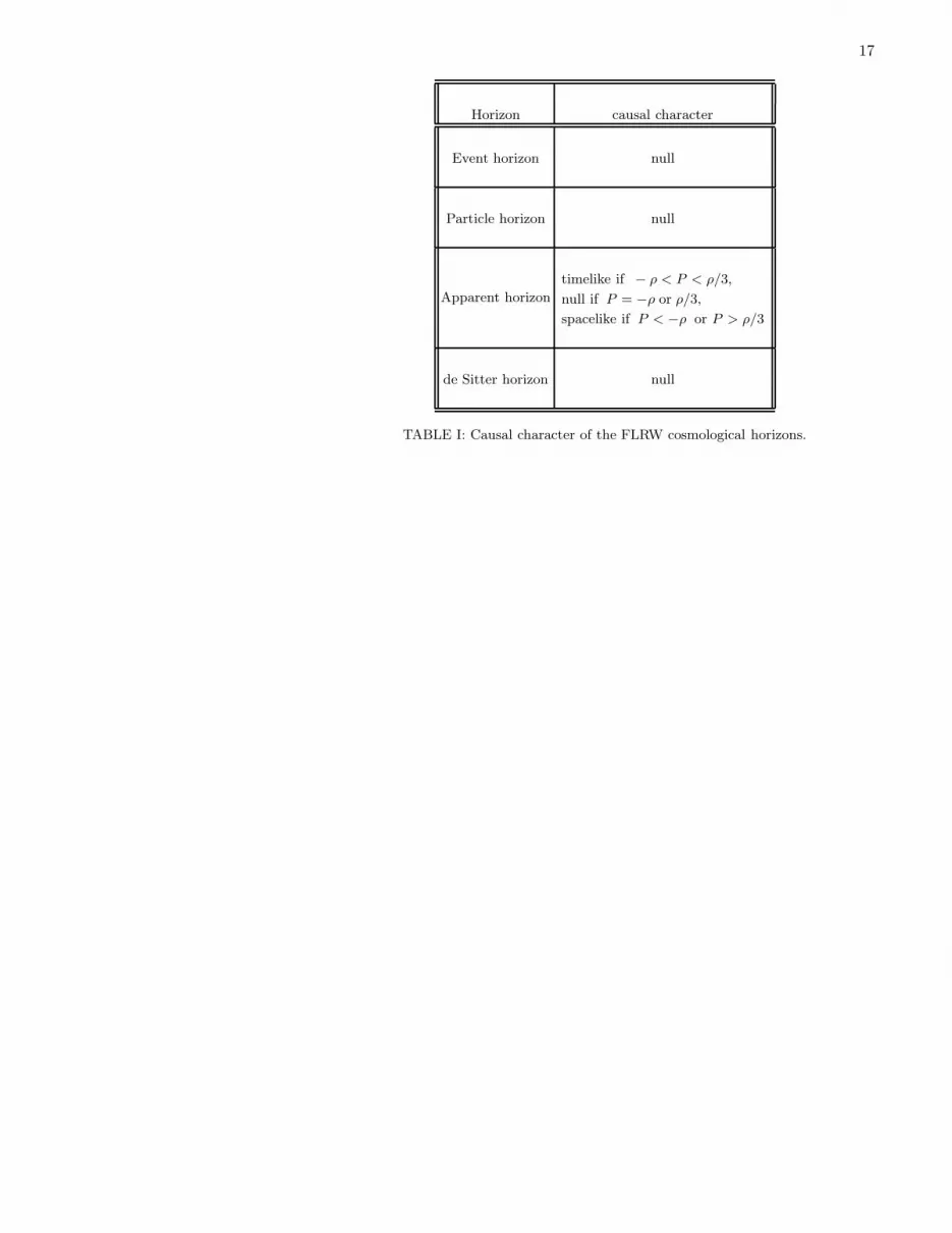
Horizon causal character

Event horizon null

Particle horizon null

Apparent horizon

timelike if − ρ < P < ρ/3,

null if P = −ρ or ρ/3,

spacelike if P < −ρ or P > ρ/3

de Sitter horizon null

TABLE I: Causal character of the FLRW cosmological horizons.

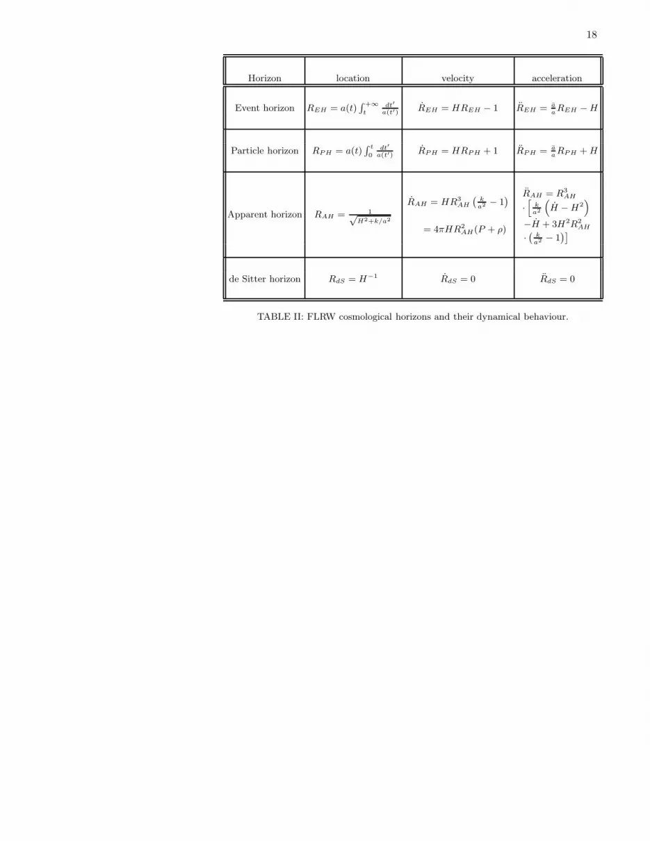
18

Horizon location velocity acceleration

Event horizon REH = a(t)∫ +∞

tdt′

a(t′)REH = HREH − 1 REH = a

aREH −H

Particle horizon RPH = a(t)∫ t

0dt′

a(t′)RPH = HRPH + 1 RPH = a

aRPH +H

Apparent horizon RAH = 1√H2+k/a2

RAH = HR3AH

(

ka2 − 1

)

= 4πHR2AH(P + ρ)

RAH = R3AH

·[

ka2

(

H −H2)

−H + 3H2R2AH

·(

ka2 − 1

)]

de Sitter horizon RdS = H−1 RdS = 0 RdS = 0

TABLE II: FLRW cosmological horizons and their dynamical behaviour.